Embed Size (px)
Citation preview

Analysis of Survey Data Using the SAS SURVEY Procedures: A Primer
Patricia A. Berglund, Institute for Social Research - University of Michigan Wisconsin and Illinois SAS User’s Group
June 25, 2014
1
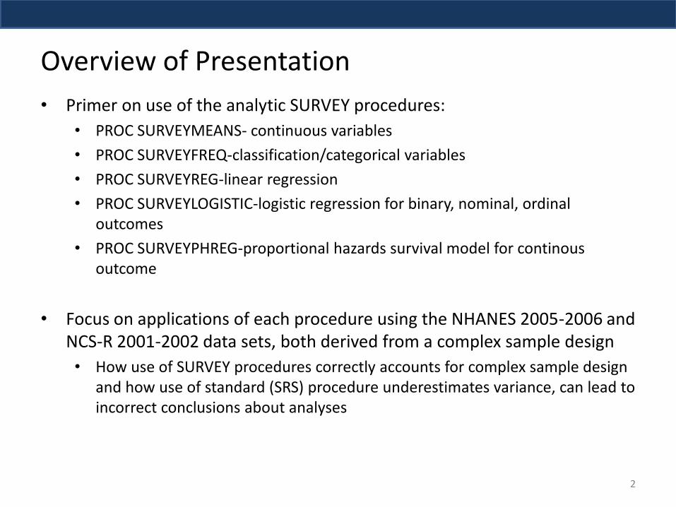
Overview of Presentation
• Primer on use of the analytic SURVEY procedures:
• PROC SURVEYMEANS- continuous variables
• PROC SURVEYFREQ-classification/categorical variables
• PROC SURVEYREG-linear regression
• PROC SURVEYLOGISTIC-logistic regression for binary, nominal, ordinal outcomes
• PROC SURVEYPHREG-proportional hazards survival model for continous outcome
• Focus on applications of each procedure using the NHANES 2005-2006 and NCS-R 2001-2002 data sets, both derived from a complex sample design
• How use of SURVEY procedures correctly accounts for complex sample design and how use of standard (SRS) procedure underestimates variance, can lead to incorrect conclusions about analyses
2
Background on Complex Sample Design Data
3
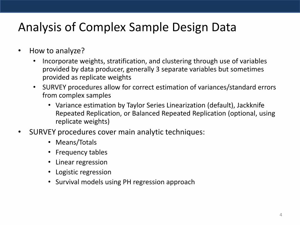
Analysis of Complex Sample Design Data
• How to analyze? • Incorporate weights, stratification, and clustering through use of variables
provided by data producer, generally 3 separate variables but sometimes provided as replicate weights
• SURVEY procedures allow for correct estimation of variances/standard errors from complex samples
• Variance estimation by Taylor Series Linearization (default), Jackknife Repeated Replication, or Balanced Repeated Replication (optional, using replicate weights)
• SURVEY procedures cover main analytic techniques: • Means/Totals
• Frequency tables
• Linear regression
• Logistic regression
• Survival models using PH regression approach
4
Why are SURVEY procedures needed?
• Use of complex sample design requires variance estimation that accounts for features such as stratification, clustering, and weights
• Most SAS procedures assume that data is from a simple random sample, assumes independence among respondents
• This is clearly not the case when using data based on a complex sample design
5
Complex Sample Survey Data: Probability Samples
• Probability sample design:
• Each population element has a known, non-zero selection probability
• Properly weighted, sample estimates are unbiased or nearly unbiased for the corresponding population statistic.
• Variance of sample statistics can be estimated from the sample data (measurability)
• Simple random sample (SRS): A probability sample in which each element has an independent and equal chance of being selected for observation. Closest population sampling analog to independently and identically distributed (iid) data.
Complex Sample Survey Data: “Complex” Designs
• “Complex sample”:
• A probability sample developed using sampling procedures such as stratification, clustering and weighting designed to improve statistical efficiency, reduce costs or improve precision for subgroup analyses relative to SRS
• Unbiased estimates with measurable sampling error are still possible
• Independence of observations, (iid), equal probabilities of selection may no longer hold
Analysis of Continuous Variables
PROC SURVEYMEANS
8
Survey Data Analysis-Continuous Variables
• Typical analyses:
• Means
• Totals
• Ratios and quantiles also possible (not shown here)
• Use PROC SURVEYMEANS for each type of analysis above
• Variance estimation via TSL, JRR, or BRR method
• Use of STRATA, CLUSTER, and WEIGHT statements (or replicate weights if supplied by data producer)
9
Analysis of Body Mass Index
• This application uses a subset of the NHANES 2005-2006 data set:
• The National Health and Nutrition Examination Survey is an ongoing health survey:
• based on a complex sample design data set
• produced by the NCHS, public release, see http://wwwn.cdc.gov/nchs/nhanes/ for details and documentation
• data set has 15 strata with 2 clusters per strata (SDMVSTR, SDMVPSU)
• weights:
• interviewed but no medical exam (WTINT2YR)
• interviewed and also participated in the medical examination (WTMEC2YR)
• The analysis focuses on estimated mean BMI among those that completed the interview and medical exam plus within selected subpopulations (domains) such as gender and marital status
10
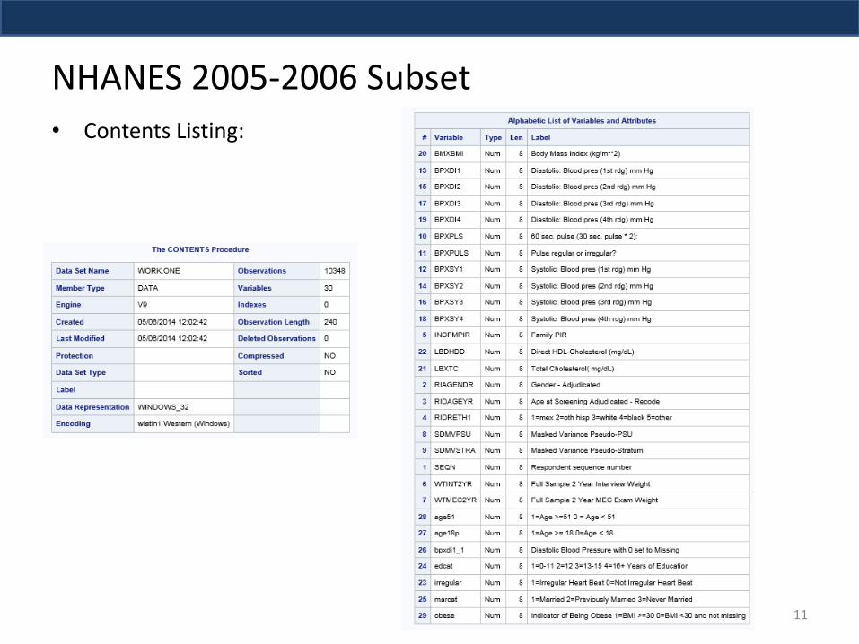
NHANES 2005-2006 Subset
• Contents Listing:
11
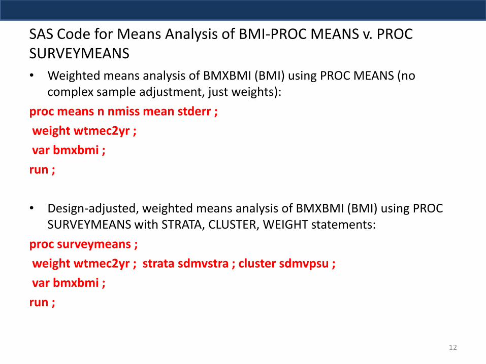
SAS Code for Means Analysis of BMI-PROC MEANS v. PROC SURVEYMEANS
• Weighted means analysis of BMXBMI (BMI) using PROC MEANS (no complex sample adjustment, just weights):
proc means n nmiss mean stderr ;
weight wtmec2yr ;
var bmxbmi ;
run ;
• Design-adjusted, weighted means analysis of BMXBMI (BMI) using PROC SURVEYMEANS with STRATA, CLUSTER, WEIGHT statements:
proc surveymeans ;
weight wtmec2yr ; strata sdmvstra ; cluster sdmvpsu ;
var bmxbmi ;
run ;
12
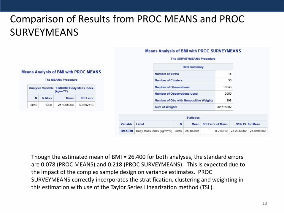
Comparison of Results from PROC MEANS and PROC SURVEYMEANS
13
Though the estimated mean of BMI = 26.400 for both analyses, the standard errors are 0.078 (PROC MEANS) and 0.218 (PROC SURVEYMEANS). This is expected due to the impact of the complex sample design on variance estimates. PROC SURVEYMEANS correctly incorporates the stratification, clustering and weighting in this estimation with use of the Taylor Series Linearization method (TSL).
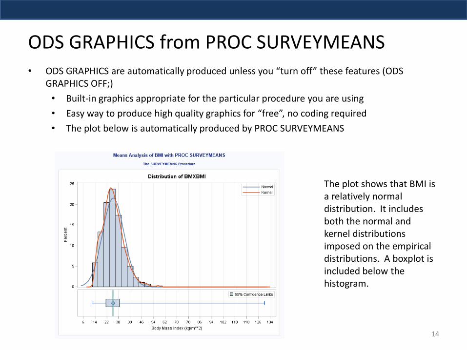
ODS GRAPHICS from PROC SURVEYMEANS • ODS GRAPHICS are automatically produced unless you “turn off” these features (ODS
GRAPHICS OFF;)
• Built-in graphics appropriate for the particular procedure you are using
• Easy way to produce high quality graphics for “free”, no coding required
• The plot below is automatically produced by PROC SURVEYMEANS
14
The plot shows that BMI is a relatively normal distribution. It includes both the normal and kernel distributions imposed on the empirical distributions. A boxplot is included below the histogram.
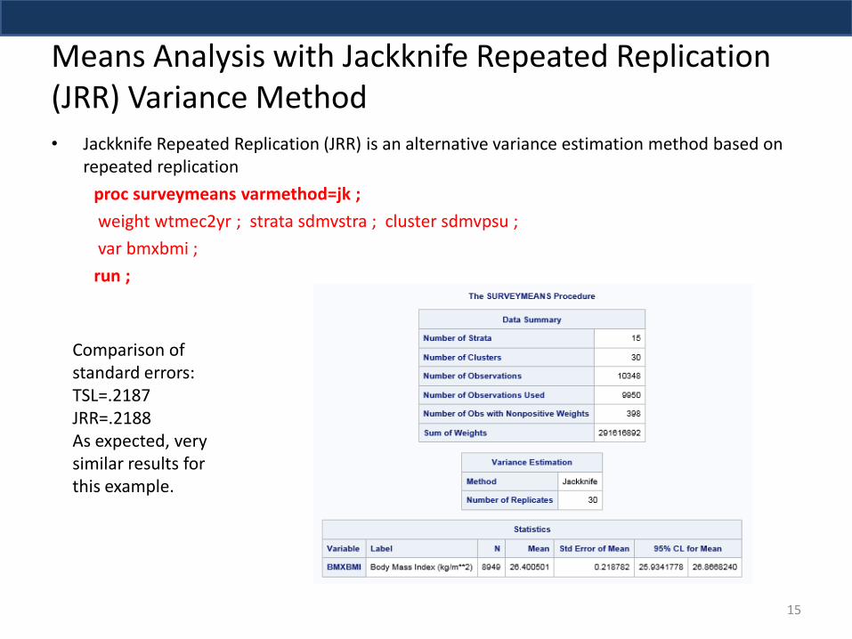
Means Analysis with Jackknife Repeated Replication (JRR) Variance Method • Jackknife Repeated Replication (JRR) is an alternative variance estimation method based on
repeated replication
proc surveymeans varmethod=jk ;
weight wtmec2yr ; strata sdmvstra ; cluster sdmvpsu ;
var bmxbmi ;
run ;
15
Comparison of standard errors: TSL=.2187 JRR=.2188 As expected, very similar results for this example.
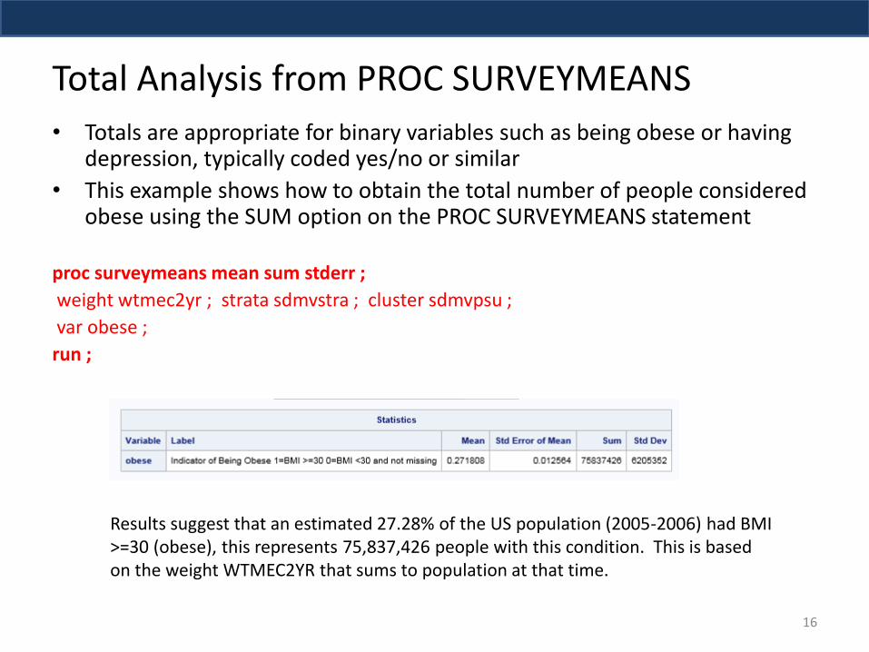
Total Analysis from PROC SURVEYMEANS
• Totals are appropriate for binary variables such as being obese or having depression, typically coded yes/no or similar
• This example shows how to obtain the total number of people considered obese using the SUM option on the PROC SURVEYMEANS statement
proc surveymeans mean sum stderr ;
weight wtmec2yr ; strata sdmvstra ; cluster sdmvpsu ;
var obese ;
run ;
16
Results suggest that an estimated 27.28% of the US population (2005-2006) had BMI >=30 (obese), this represents 75,837,426 people with this condition. This is based on the weight WTMEC2YR that sums to population at that time.
Domain Analysis of BMI • A common analytic task is estimation of a statistics among subpopulations or
domains, • Subpopulation analyses must be done with a DOMAIN statement rather than a
BY/WHERE statement, why? • From the SAS PROC SURVEYMEANS documentation (SAS/STAT 13.1): • “The formation of these domains might be unrelated to the sample design.
Therefore, the sample sizes for the domains are random variables. Use a DOMAIN statement to incorporate this variability into the variance estimation. Note that a DOMAIN statement is different from a BY statement. In a BY statement, you treat the sample sizes as fixed in each subpopulation, and you perform analysis within each BY group independently.”
• SAS code for a correct domain analysis of BMI by gender:
proc surveymeans ; weight wtmec2yr ; strata sdmvstra ; cluster sdmvpsu ; var bmxbmi ; domain riagendr ; format riagendr sexf. ; run ;
17
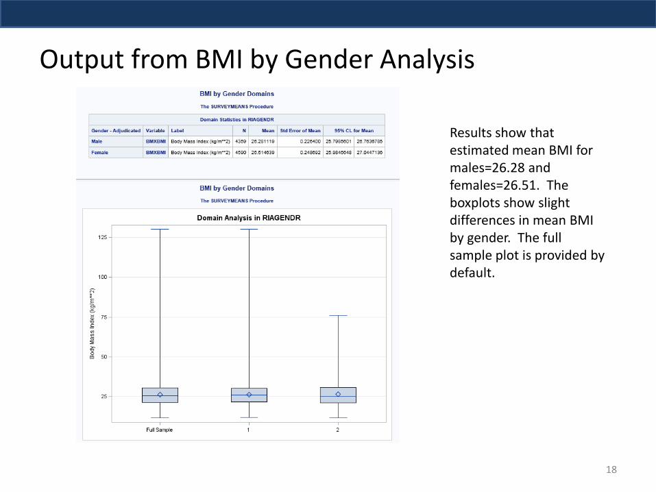
Output from BMI by Gender Analysis
18
Results show that estimated mean BMI for males=26.28 and females=26.51. The boxplots show slight differences in mean BMI by gender. The full sample plot is provided by default.
Linear Contrasts of Mean BMI by Marital Status
• PROC SURVEYMEANS does not offer a built-in command to perform a linear contrast or difference in means, therefore use of PROC SURVEYREG with a CONTRAST statement is demonstrated for a test of significant differences in mean BMI by marital status
• This test can also be done with LSMEANS/DIFF in PROC SURVEYREG (more on this in the next section)
• Another slightly out of date but still good option is the SAS Institute macro called %smsub (support.sas.com)
• This provides a macro which produces contrasts much like the PROC SURVEYREG method demonstrated here
19
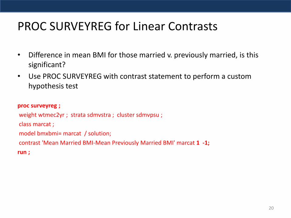
PROC SURVEYREG for Linear Contrasts
• Difference in mean BMI for those married v. previously married, is this significant?
• Use PROC SURVEYREG with contrast statement to perform a custom hypothesis test
proc surveyreg ;
weight wtmec2yr ; strata sdmvstra ; cluster sdmvpsu ;
class marcat ;
model bmxbmi= marcat / solution;
contrast 'Mean Married BMI-Mean Previously Married BMI' marcat 1 -1;
run ;
20
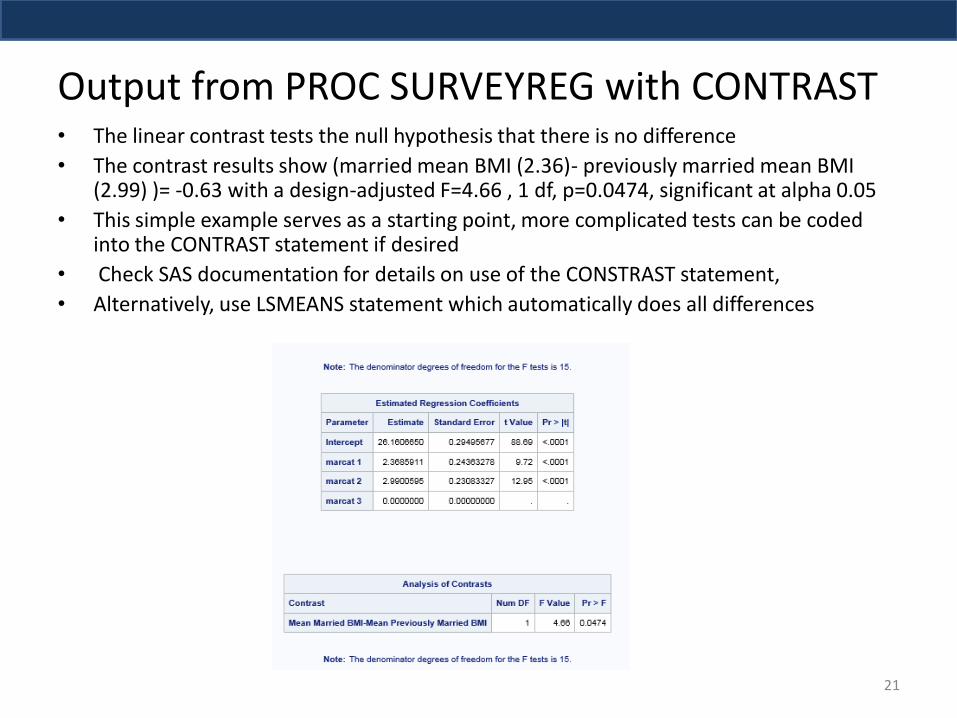
Output from PROC SURVEYREG with CONTRAST • The linear contrast tests the null hypothesis that there is no difference
• The contrast results show (married mean BMI (2.36)- previously married mean BMI (2.99) )= -0.63 with a design-adjusted F=4.66 , 1 df, p=0.0474, significant at alpha 0.05
• This simple example serves as a starting point, more complicated tests can be coded into the CONTRAST statement if desired
• Check SAS documentation for details on use of the CONSTRAST statement,
• Alternatively, use LSMEANS statement which automatically does all differences
21
Analysis of Classification Variables
PROC SURVEYFREQ
22
Frequency Tables and PROC SURVEYFREQ
• PROC SURVEYFREQ produces complex sample design adjusted variance estimates and hypothesis tests for one-way and multi-way tables
• Subpopulation analyses are done with an “implied” domain variable approach by listing the domain variable FIRST in TABLES statement
• Demonstrations include tables analysis of marital status, gender and obesity
23
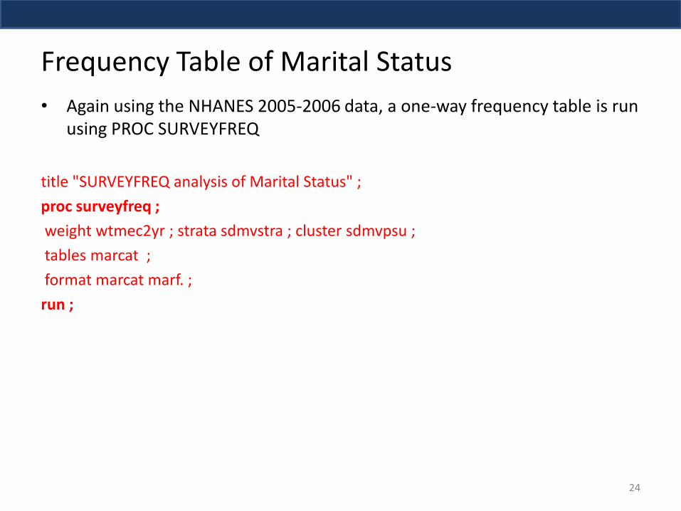
Frequency Table of Marital Status
• Again using the NHANES 2005-2006 data, a one-way frequency table is run using PROC SURVEYFREQ
title "SURVEYFREQ analysis of Marital Status" ;
proc surveyfreq ;
weight wtmec2yr ; strata sdmvstra ; cluster sdmvpsu ;
tables marcat ;
format marcat marf. ;
run ;
24
Output from PROC SURVEYFREQ Analysis of Marital Status
25
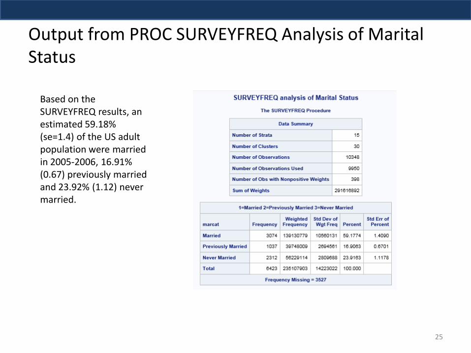
Based on the SURVEYFREQ results, an estimated 59.18% (se=1.4) of the US adult population were married in 2005-2006, 16.91% (0.67) previously married and 23.92% (1.12) never married.
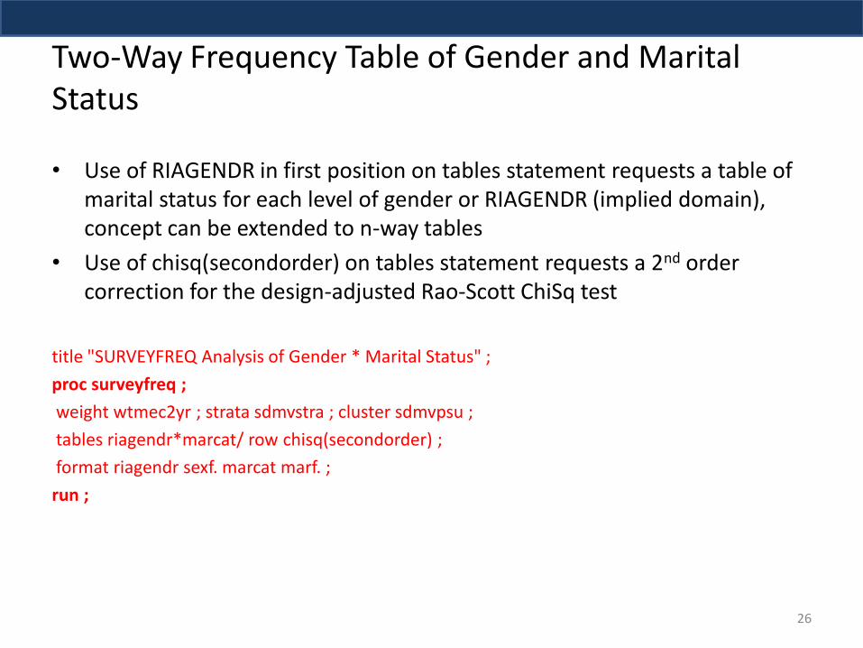
Two-Way Frequency Table of Gender and Marital Status
• Use of RIAGENDR in first position on tables statement requests a table of marital status for each level of gender or RIAGENDR (implied domain), concept can be extended to n-way tables
• Use of chisq(secondorder) on tables statement requests a 2nd order correction for the design-adjusted Rao-Scott ChiSq test
title "SURVEYFREQ Analysis of Gender * Marital Status" ;
proc surveyfreq ;
weight wtmec2yr ; strata sdmvstra ; cluster sdmvpsu ;
tables riagendr*marcat/ row chisq(secondorder) ;
format riagendr sexf. marcat marf. ;
run ;
26
Output for Gender * Marital Status Frequency Table
27
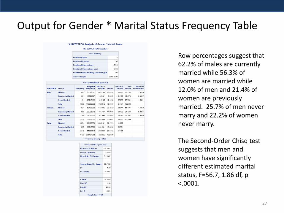
Row percentages suggest that 62.2% of males are currently married while 56.3% of women are married while 12.0% of men and 21.4% of women are previously married. 25.7% of men never marry and 22.2% of women never marry. The Second-Order Chisq test suggests that men and women have significantly different estimated marital status, F=56.7, 1.86 df, p <.0001.
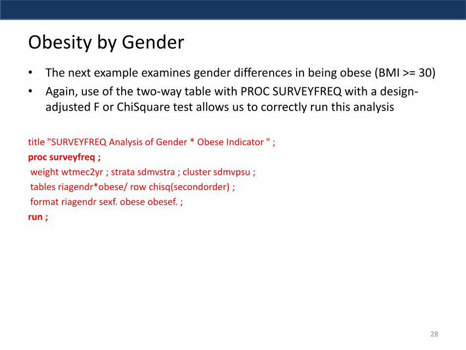
Obesity by Gender
• The next example examines gender differences in being obese (BMI >= 30)
• Again, use of the two-way table with PROC SURVEYFREQ with a design-adjusted F or ChiSquare test allows us to correctly run this analysis
title "SURVEYFREQ Analysis of Gender * Obese Indicator " ;
proc surveyfreq ;
weight wtmec2yr ; strata sdmvstra ; cluster sdmvpsu ;
tables riagendr*obese/ row chisq(secondorder) ;
format riagendr sexf. obese obesef. ;
run ;
28
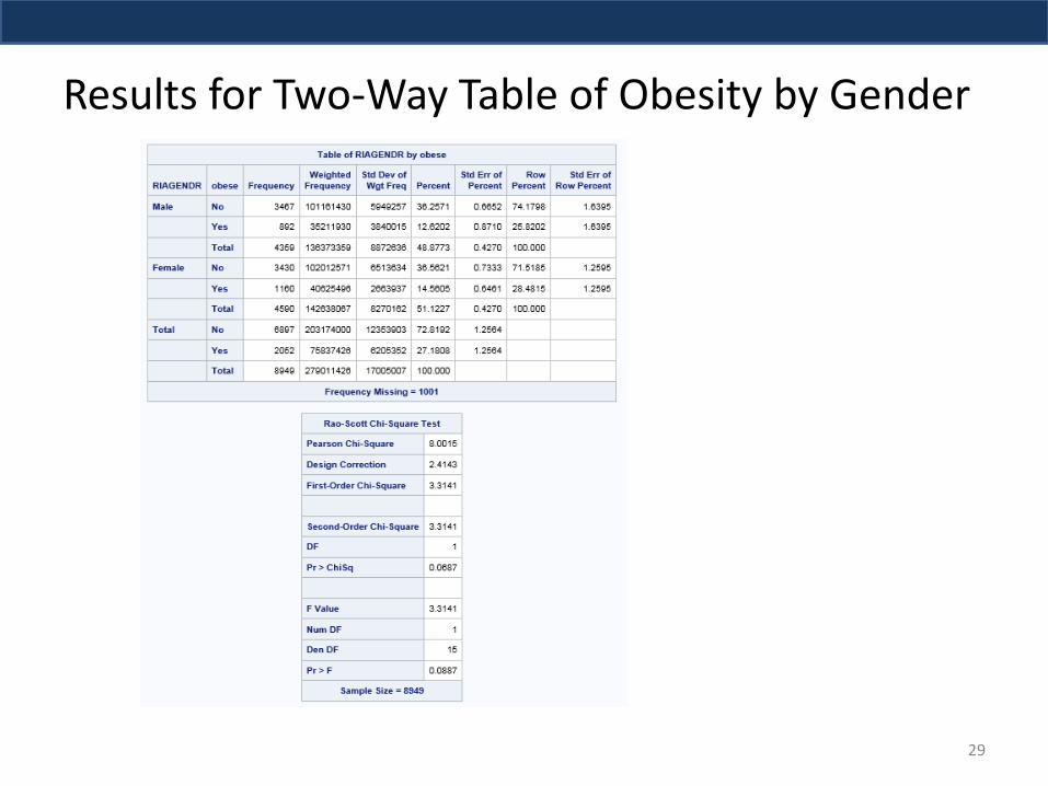
Results for Two-Way Table of Obesity by Gender
29
Linear Regression Analysis
PROC SURVEYREG
30
Linear Regression with PROC SURVEYREG
• PROC SURVEYREG is the survey data analysis equivalent of PROC REG and other linear modeling procedures (PROC MIXED, PROC GLM, PROC GENMOD)
• This tool provides the ability to perform linear regression with many optional statements such as CLASS, CONTRAST, DOMAIN, LSMEANS, and so on (PROC SURVEYREG help details each statement)
• As with other SURVEY procedures, use of the STRATA, CLUSTER, WEIGHT statements incorporates the complex sample design stratification, clustering, and weights
• For subpopulation or domain analysis, use of the DOMAIN statement correctly performs a subpopulation analysis as well as a full sample analysis
31
Linear Regression Analysis of Systolic Blood Pressure
• This example focuses on a linear regression of systolic blood pressure regressed on obesity status and education
• Use of PROC SURVEYREG with selected optional statements
• The analytic goal is to examine blood pressure within the subpopulation of those 40 and older, therefore use of a DOMAIN statement is required
• In data step prior to regression, an indicator of age 40+ is created:
if ridageyr >= 40 then age40p=1; else age40p=0; (note: no missing data on age)
32
Linear Regression with PROC SURVEYREG
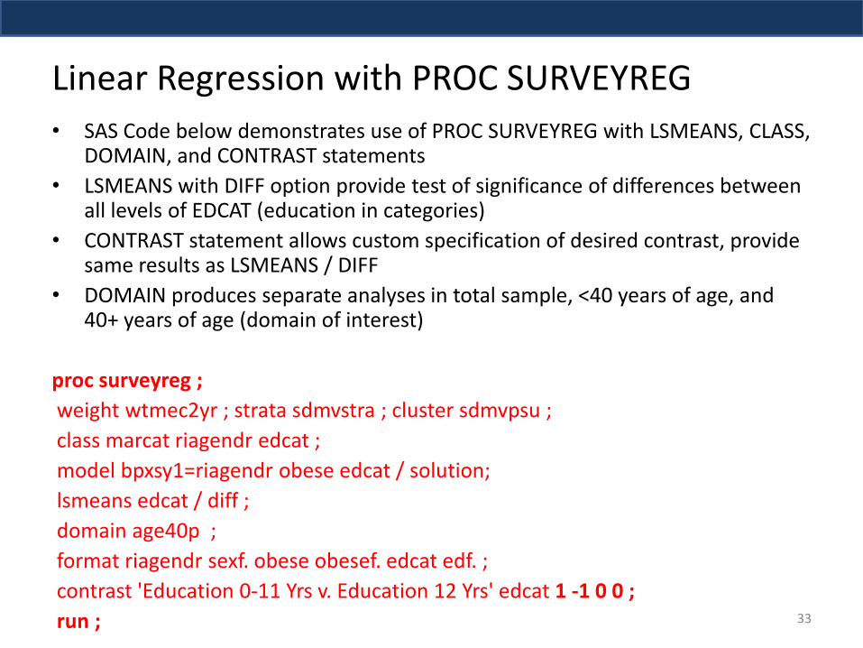
• SAS Code below demonstrates use of PROC SURVEYREG with LSMEANS, CLASS, DOMAIN, and CONTRAST statements
• LSMEANS with DIFF option provide test of significance of differences between all levels of EDCAT (education in categories)
• CONTRAST statement allows custom specification of desired contrast, provide same results as LSMEANS / DIFF
• DOMAIN produces separate analyses in total sample, <40 years of age, and 40+ years of age (domain of interest)
proc surveyreg ;
weight wtmec2yr ; strata sdmvstra ; cluster sdmvpsu ;
class marcat riagendr edcat ;
model bpxsy1=riagendr obese edcat / solution;
lsmeans edcat / diff ;
domain age40p ;
format riagendr sexf. obese obesef. edcat edf. ;
contrast 'Education 0-11 Yrs v. Education 12 Yrs' edcat 1 -1 0 0 ;
run ; 33
PROC SURVEYREG Output for Subpopulation of Those Age 40+
34
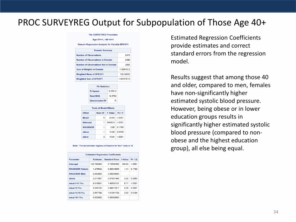
Estimated Regression Coefficients provide estimates and correct standard errors from the regression model. Results suggest that among those 40 and older, compared to men, females have non-significantly higher estimated systolic blood pressure. However, being obese or in lower education groups results in significantly higher estimated systolic blood pressure (compared to non-obese and the highest education group), all else being equal.
PROC SURVEYREG Output for Subpopulation of Those Age 40+
35
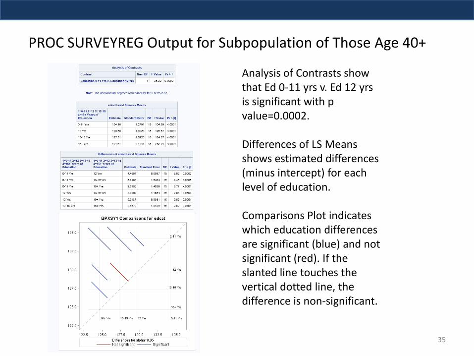
Analysis of Contrasts show that Ed 0-11 yrs v. Ed 12 yrs is significant with p value=0.0002. Differences of LS Means shows estimated differences (minus intercept) for each level of education. Comparisons Plot indicates which education differences are significant (blue) and not significant (red). If the slanted line touches the vertical dotted line, the difference is non-significant.
PROC SURVEYREG Output, continued
• Output displayed in previous slide was just for those in subpopulation of interest, age 40+ but the same output is displayed for total sample and also those < 40 years of age, check statement at the top of the output to determine which population is used
• What if we had not used PROC SURVEYREG but used PROC MIXED instead, would this alter our overall conclusions?
36
Linear Regression with PROC MIXED
37
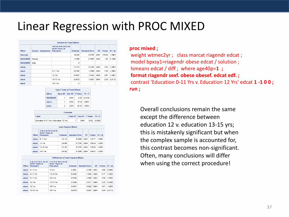
proc mixed ; weight wtmec2yr ; class marcat riagendr edcat ; model bpxsy1=riagendr obese edcat / solution ; lsmeans edcat / diff ; where age40p=1 ; format riagendr sexf. obese obesef. edcat edf. ; contrast 'Education 0-11 Yrs v. Education 12 Yrs' edcat 1 -1 0 0 ; run ;
Overall conclusions remain the same except the difference between education 12 v. education 13-15 yrs; this is mistakenly significant but when the complex sample is accounted for, this contrast becomes non-significant. Often, many conclusions will differ when using the correct procedure!
Logistic Regression
PROC SURVEYLOGISTIC
38
Logistic Regression
• PROC SURVEYLOGISTIC is the tool for a variety of logistic regression with outcomes such as:
• Binary
• Ordinal
• Nominal
• The different types of logistic regression can be requested through use of the LINK option on the MODEL statement
• Other optional statements are:
• CLASS
• DOMAIN
• TEST
• CONTRAST
• LSMEAN and so on
39
PROC LOGISTIC with Binary Outcome
• Logistic regression with a binary outcome is a common use of PROC LOGISTIC/SURVEYLOGISTIC
• This example uses the NCS-R data
• NCS-R (National Comorbidity Survey-Replication, 2001-2003, Dr. Ronald Kessler) is a nationally representative data set focused on mental health diagnoses, treatment, and other socio-demographic issues, see http://www.hcp.med.harvard.edu/ncs/ for more information
40
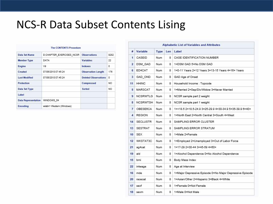
NCS-R Data Subset Contents Lising
41
Analysis of Major Depressive Episode with PROC SURVEYLOGISTIC – Binary Outcome
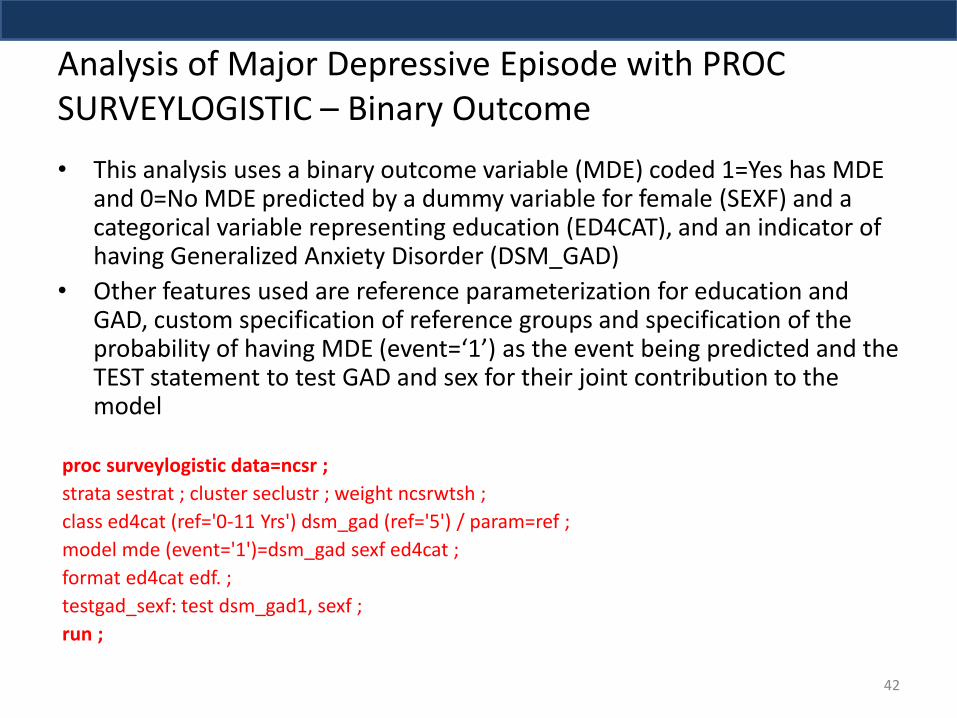
• This analysis uses a binary outcome variable (MDE) coded 1=Yes has MDE and 0=No MDE predicted by a dummy variable for female (SEXF) and a categorical variable representing education (ED4CAT), and an indicator of having Generalized Anxiety Disorder (DSM_GAD)
• Other features used are reference parameterization for education and GAD, custom specification of reference groups and specification of the probability of having MDE (event=‘1’) as the event being predicted and the TEST statement to test GAD and sex for their joint contribution to the model
proc surveylogistic data=ncsr ;
strata sestrat ; cluster seclustr ; weight ncsrwtsh ;
class ed4cat (ref='0-11 Yrs') dsm_gad (ref='5') / param=ref ;
model mde (event='1')=dsm_gad sexf ed4cat ;
format ed4cat edf. ;
testgad_sexf: test dsm_gad1, sexf ;
run ;
42
Selected Output from PROC SURVEYLOGISTIC
43
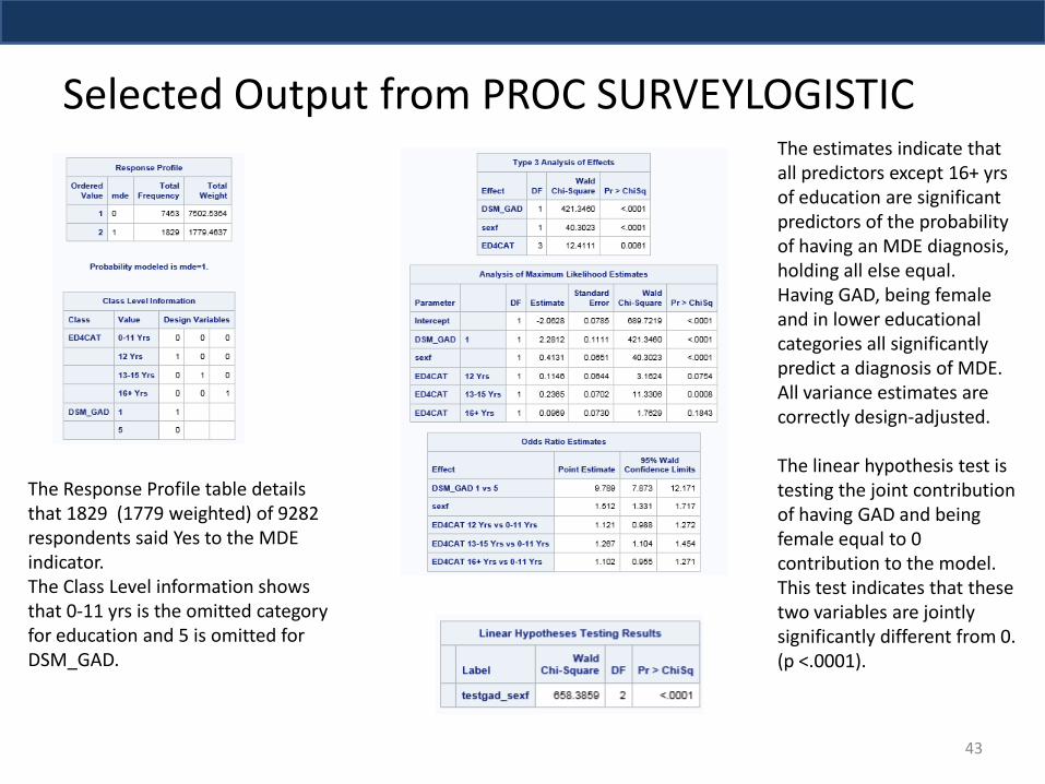
The Response Profile table details that 1829 (1779 weighted) of 9282 respondents said Yes to the MDE indicator. The Class Level information shows that 0-11 yrs is the omitted category for education and 5 is omitted for DSM_GAD.
The estimates indicate that all predictors except 16+ yrs of education are significant predictors of the probability of having an MDE diagnosis, holding all else equal. Having GAD, being female and in lower educational categories all significantly predict a diagnosis of MDE. All variance estimates are correctly design-adjusted. The linear hypothesis test is testing the joint contribution of having GAD and being female equal to 0 contribution to the model. This test indicates that these two variables are jointly significantly different from 0. (p <.0001).
Analysis of Marital Status (Nominal Outcome) with PROC SURVEYLOGISTIC
• With marital status as the nominal outcome, use of the LINK=GLOGIT option on the MODEL statement is needed to produce a multinomial logistic regression
• default is LINK=LOGIT for PROC SURVEYLOGISTIC
• This example uses the same basic setup as the previous example but adds the correct link option to predict marital status category with education (4 categories)
proc surveylogistic data=ncsr ;
strata sestrat ; cluster seclustr ; weight ncsrwtsh ;
class ed4cat / param=ref ;
model mar3cat =ed4cat / link=glogit ;
format ed4cat edf. Format mar3cat marf. ;
run ;
44
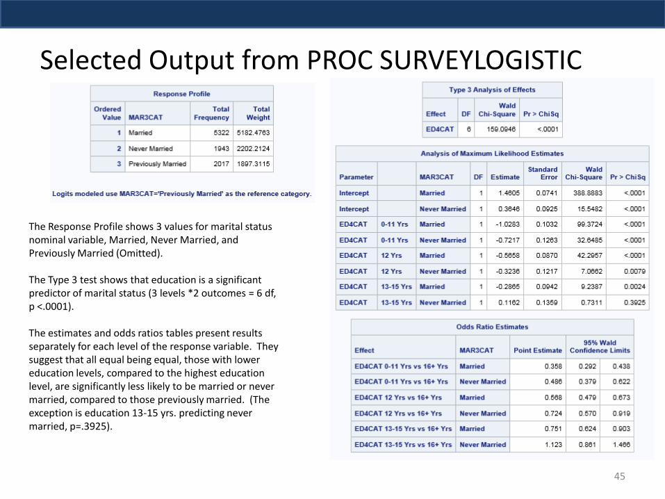
Selected Output from PROC SURVEYLOGISTIC
45
The Response Profile shows 3 values for marital status nominal variable, Married, Never Married, and Previously Married (Omitted). The Type 3 test shows that education is a significant predictor of marital status (3 levels *2 outcomes = 6 df, p <.0001). The estimates and odds ratios tables present results separately for each level of the response variable. They suggest that all equal being equal, those with lower education levels, compared to the highest education level, are significantly less likely to be married or never married, compared to those previously married. (The exception is education 13-15 yrs. predicting never married, p=.3925).
Additional Features of PROC SURVEYLOGISTIC
• Many other features are available but not presented here:
• Ordinal logistic regression (outcome > 2 categories with order)
• LSMEANS, LSMESTIMATES, DOMAIN, UNIT, ODS GRAPHICS, CONTRAST, EFFECT, and so on (see SAS/STAT 13.1 documentation for more)
• Another important option is the NOMCAR (Not Missing Completely at Random), allows creating a separate domain of the cases with missing data, enables comparisons with complete cases and analyzes missing data as a domain of its own
46
Survival Analysis Using Cox Model (Proportional Hazards)
PROC SURVEYPHREG
47
Features of Survival Analysis
• Survival analysis is focused on time and censoring
• Time to event of interest such as
• Disease onset
• Death
• Engine failure
• Measurement of time
• Continuous time (seconds, days)
• Discrete time units (2 year periods, decades)
• Censoring
• No event of interest during time observed, considered censored (lost to follow-up)
• Left and right censoring
Event History Data
• Longitudinal data
• Prospectively collected on individuals followed over time (Panel Study for Income Dynamics)
• Administrative follow-up data
• Administrative records used to link to additional survey data, prospectively follows those individuals to a key event such as death (NHANES III linked mortality file: http://cdc.gov/nchs/data/datalinkage)
• Retrospective data
• Respondents asked to recall details about an event of interest which occurred at some point in the past (NCS-R)
Cox Proportional Hazards Model
• Cox PH models are considered semi-parametric, assumes continuous time with proportional hazards among covariates
• Use of PROC SURVEYPHREG for Cox model fitting with complex sample survey data is demonstrated
• Data used is NCS-R but requires a few special variables measuring time intervals between events of interest
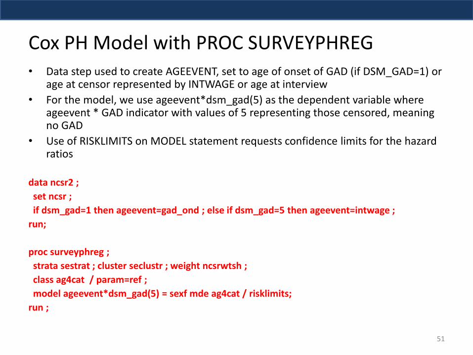
Cox PH Model with PROC SURVEYPHREG • Data step used to create AGEEVENT, set to age of onset of GAD (if DSM_GAD=1) or
age at censor represented by INTWAGE or age at interview
• For the model, we use ageevent*dsm_gad(5) as the dependent variable where ageevent * GAD indicator with values of 5 representing those censored, meaning no GAD
• Use of RISKLIMITS on MODEL statement requests confidence limits for the hazard ratios
data ncsr2 ;
set ncsr ;
if dsm_gad=1 then ageevent=gad_ond ; else if dsm_gad=5 then ageevent=intwage ;
run;
proc surveyphreg ;
strata sestrat ; cluster seclustr ; weight ncsrwtsh ;
class ag4cat / param=ref ;
model ageevent*dsm_gad(5) = sexf mde ag4cat / risklimits;
run ;
51
Output from PROC SURVEYPHREG
• Default output from PROC SURVEYPHREG includes the hazard ratio
• hazard ratio is the probability that an event will occur at time t, given that it has not yet occurred (a conditional probability)
• What does it mean?
• Hazard ratio for a given predictor represents the impact that a one unit change in that predictor will have on the expected hazard
• For categorical predictors, the one unit change in a predictor is compared to the omitted reference category
52
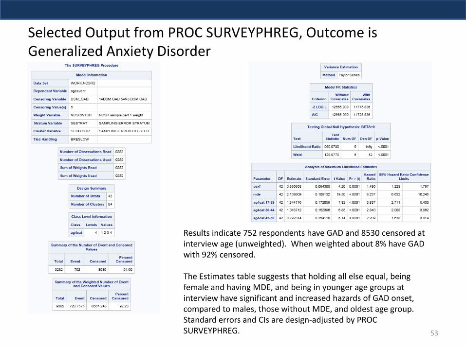
Selected Output from PROC SURVEYPHREG, Outcome is Generalized Anxiety Disorder
53
Results indicate 752 respondents have GAD and 8530 censored at interview age (unweighted). When weighted about 8% have GAD with 92% censored. The Estimates table suggests that holding all else equal, being female and having MDE, and being in younger age groups at interview have significant and increased hazards of GAD onset, compared to males, those without MDE, and oldest age group. Standard errors and CIs are design-adjusted by PROC SURVEYPHREG.
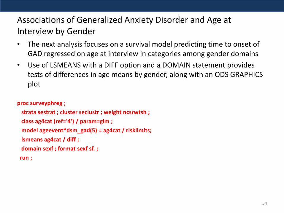
Associations of Generalized Anxiety Disorder and Age at Interview by Gender
• The next analysis focuses on a survival model predicting time to onset of GAD regressed on age at interview in categories among gender domains
• Use of LSMEANS with a DIFF option and a DOMAIN statement provides tests of differences in age means by gender, along with an ODS GRAPHICS plot
proc surveyphreg ;
strata sestrat ; cluster seclustr ; weight ncsrwtsh ;
class ag4cat (ref='4') / param=glm ;
model ageevent*dsm_gad(5) = ag4cat / risklimits;
lsmeans ag4cat / diff ;
domain sexf ; format sexf sf. ;
run ;
54
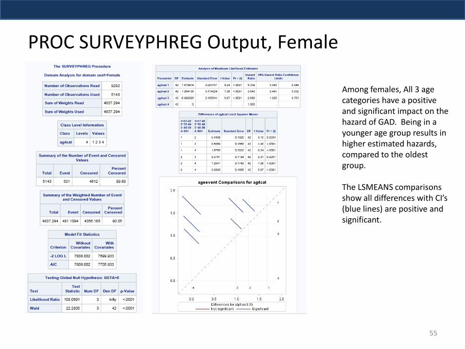
PROC SURVEYPHREG Output, Female
55
Among females, All 3 age categories have a positive and significant impact on the hazard of GAD. Being in a younger age group results in higher estimated hazards, compared to the oldest group. The LSMEANS comparisons show all differences with CI’s (blue lines) are positive and significant.

PROC SURVEYPHREG, Male
56
Among males, All 3 age categories have a positive and significant impact on the hazard of GAD, as compared to the omitted oldest age group. The LSMEANS comparisons show only about half (blue lines) of the differences are significant with the each age group v. the oldest age group significant but the other comparisons non-significant (red lines that cross the 45 degree imposed line). The DOMAIN analysis reveals gender differences in age at interview predicting the hazard of a GAD diagnosis.
Presentation Summary • This presentation has covered the main analytic procedures in the SURVEY
group: • PROC SURVEYMEANS • PROC SURVEYFREQ • PROC SURVEYREG • PROC SURVEYLOGISTIC • PROC SURVEYPHREG
• A variety of optional statements/features have been covered: • DOMAIN • TEST • LSMEANS • CONTRAST • ODS GRAPHICS • Comparison of results to Simple Random Sample based results
• Much more can be done with the SURVEY procedures, see SAS/STAT
documentation and additional resources
57
Additional Resources and References • SAS/STAT documentation and conference papers
• “Applied Survey Data Analysis” Heeringa, West, and Berglund (2010)
• Website for “Applied Survey Data Analysis” http://www.isr.umich.edu/src/smp/asda/
• IDRE/UCLA https://idre.ucla.edu/stats
• Korn, E. L. and Graubard, B. I. (1999), Analysis of Health Surveys, New York: John Wiley & Sons.
• Rust, K. (1985), “Variance Estimation for Complex Estimators in Sample Surveys,” Journal of Official Statistics, 1, 381–397.
• Lee, E. S., Forthofer, R. N., and Lorimor, R. J. (1989), Analyzing Complex Survey Data, Sage University Paper Series on Quantitative Applications in the Social Sciences, 07-071, Beverly Hills, CA: Sage Publications.
58

Author Contact Information
• Your comments and feedback are welcome and thank you for attending today!
• Patricia Berglund
59