Analysis of Stroke on Brain Computed Tomography Scans

Thesis submitted in partial fulfillment

of the requirements for the degree of

M.S.

in

Computer Science

by

Saurabh Sharma

200502024saurabhsharma@research.iiit.ac.in

Center for Visual Information Technology

International Institute of Information Technology

Hyderabad - 500 032, INDIA

October 2013

Copyright c© Saurabh Sharma, 2013

All Rights Reserved

International Institute of Information Technology

Hyderabad, India

CERTIFICATE

It is certified that the work contained in this thesis, titled“Analysis of Stroke on Brain Computed To-

mography Scans” by Saurabh Sharma, has been carried out under my supervision and is not submitted

elsewhere for a degree.

Date Adviser: Prof. Jayanthi Sivaswamy

To MY PARENTS

Abstract

Stroke is one of the leading causes of death and disability inthe world. Early detection of Stroke

(both hemorrhagic and ischemic) is very important as it can ensure up to full recovery. Timely detection

of stroke, especially ischemic stroke is difficult as the changes in abnormal tissue only become visible

after the damage has already been done. The detection is evenmore difficult on CT scan compared to

other imaging modalities but the dependence of a large fraction of population on CT, makes the need

to find a solution to the problem even more imperative. Thoughthe detection accuracy of radiologists

for early stroke depends on various factors like experience, available technology, etc., earlier estimates

put the accuracy around 10% [45]. Even with considerable advancement in CT technology the perfor-

mance has still only increased to around 70% or thereabouts [21]. Any kind of assistance to radiologists

which can improve their detection accuracy would thereforebe much appreciated. This thesis presents

a framework for automatic detection and classification of different types of stroke. We characterize

stroke as a distortion in the otherwise contralaterally similar distribution of brain tissue. Classification

depends on the severity of the distortion with hemorrhage and chronic infarcts exhibiting the maximum

distortion and hyperacute stroke showing the minimum. The detection work on hemorrhagic stroke and

early ischemic stroke has clinical value whereas the work onlater stages of ischemic stroke has mainly

academic use. The automatic detection approach was tested on a dataset containing 19 normal (291

slices) and 23 abnormal (181 slices) datasets. The algorithm gave a high recall rate for hemorrhage

(80%), chronic (95%), acute (91.80%) and hyperacute (82.22%) stroke at slice level. The correspond-

ing precision figures were 93.3%, 90.47%, 87.5% and 69.81% respectively. The performance of the

system in a normal vs. stroke-affected scenario was 83.95% precision and 86.74% recall. The lower

precision value in case of hyperacute scans is because of large number of normal slices with slight dis-

turbances in contra-lateral symmetry being identified as stroke cases. We also present a novel approach

for enhancement of early ischemic stroke regions using image-adaptive window parameters, to aid the

radiologists in the manual detection of early ischemic stroke. The enhancement approach increased

the average accuracy of radiologists in clinical conditions from around 71% to around 90% (p=0.02,

two tailed student’s t test) with the inexperienced radiologists benefitting more from the enhancement.

The average reviewing time of the scans was also reduced fromabout 9 to 6 seconds per slice. Out of

the two approaches, automatic detection and enhancement, results show the enhancement process to be

more promising.

v

Contents

Chapter Page

1 Introduction . . . . . . . . . . . . . . . . . . . . . . . . . . . . . . . . . . . . . . . . . . 11.1 Medical Background . . . . . . . . . . . . . . . . . . . . . . . . . . . . . . .. . . . 2

1.1.1 Human Brain . . . . . . . . . . . . . . . . . . . . . . . . . . . . . . . . . . . 21.1.2 Brain Stroke . . . . . . . . . . . . . . . . . . . . . . . . . . . . . . . . . . . 21.1.3 Imaging the Brain . . . . . . . . . . . . . . . . . . . . . . . . . . . . . . .. 31.1.4 Stroke in Brain CT . . . . . . . . . . . . . . . . . . . . . . . . . . . . . . .. 5

1.2 Why Unenhanced CT . . . . . . . . . . . . . . . . . . . . . . . . . . . . . . . . .. . 71.3 Earliest Visible Signs of Acute Infarct . . . . . . . . . . . . . .. . . . . . . . . . . . 71.4 Problem Statement and Contribution . . . . . . . . . . . . . . . . .. . . . . . . . . . 9

1.4.1 Track 1 . . . . . . . . . . . . . . . . . . . . . . . . . . . . . . . . . . . . . . 91.4.2 Track 2 . . . . . . . . . . . . . . . . . . . . . . . . . . . . . . . . . . . . . . 10

1.5 Thesis Structure . . . . . . . . . . . . . . . . . . . . . . . . . . . . . . . . .. . . . . 10

2 Related Work . . . . . . . . . . . . . . . . . . . . . . . . . . . . . . . . . . . . . . . . . 122.1 Hemorrhage Detection . . . . . . . . . . . . . . . . . . . . . . . . . . . . .. . . . . 122.2 Ischemic Stroke . . . . . . . . . . . . . . . . . . . . . . . . . . . . . . . . . .. . . . 132.3 Ischemic Stroke Enhancement . . . . . . . . . . . . . . . . . . . . . . .. . . . . . . 14

3 Automatic Stroke Detection. . . . . . . . . . . . . . . . . . . . . . . . . . . . . . . . . . 163.1 Preprocessing . . . . . . . . . . . . . . . . . . . . . . . . . . . . . . . . . . .. . . . 163.2 Mid-Sagittal Plane Detection and Rotation Correction .. . . . . . . . . . . . . . . . . 173.3 Stroke Detection and Identification . . . . . . . . . . . . . . . . .. . . . . . . . . . . 19

3.3.1 Level 1 Classification . . . . . . . . . . . . . . . . . . . . . . . . . . .. . . . 193.3.2 Level 2 Classification . . . . . . . . . . . . . . . . . . . . . . . . . . .. . . . 193.3.3 Level 3 Classification . . . . . . . . . . . . . . . . . . . . . . . . . . .. . . . 20

3.3.3.1 Contrast Enhancement . . . . . . . . . . . . . . . . . . . . . . . . .233.3.3.2 Tissue Segmentation . . . . . . . . . . . . . . . . . . . . . . . . . .243.3.3.3 Candidate Selection . . . . . . . . . . . . . . . . . . . . . . . . . .253.3.3.4 Hyperacute Infarct Region Detection . . . . . . . . . . . .. . . . . 26

3.4 Results and Discussion . . . . . . . . . . . . . . . . . . . . . . . . . . . .. . . . . . 263.4.1 Dataset Details . . . . . . . . . . . . . . . . . . . . . . . . . . . . . . . .. . 263.4.2 Detection Results and Discussion . . . . . . . . . . . . . . . . .. . . . . . . 27

vi

CONTENTS vii

4 Enhancement of Early Infarct through Auto-Windowing. . . . . . . . . . . . . . . . . . . . 324.1 Manual Windowing . . . . . . . . . . . . . . . . . . . . . . . . . . . . . . . . .. . . 324.2 Region Based Windowing . . . . . . . . . . . . . . . . . . . . . . . . . . . .. . . . 364.3 Pixel Based Windowing . . . . . . . . . . . . . . . . . . . . . . . . . . . . .. . . . . 36

4.3.0.1 Parzen Window . . . . . . . . . . . . . . . . . . . . . . . . . . . . 374.3.0.2 Parzen Based Windowing . . . . . . . . . . . . . . . . . . . . . . . 38

4.4 Results . . . . . . . . . . . . . . . . . . . . . . . . . . . . . . . . . . . . . . . . .. . 394.4.1 Experiment Details . . . . . . . . . . . . . . . . . . . . . . . . . . . . .. . . 394.4.2 Discussion . . . . . . . . . . . . . . . . . . . . . . . . . . . . . . . . . . . .40

5 Conclusions . . . . . . . . . . . . . . . . . . . . . . . . . . . . . . . . . . . . . . . . . . 425.1 Automatic Detection . . . . . . . . . . . . . . . . . . . . . . . . . . . . . .. . . . . 425.2 Enhancement of Affected Tissue . . . . . . . . . . . . . . . . . . . . .. . . . . . . . 43

Bibliography . . . . . . . . . . . . . . . . . . . . . . . . . . . . . . . . . . . . . . . . . . . . 46

List of Figures

Figure Page

1.1 Axial view of gray and white matter [38] . . . . . . . . . . . . . . .. . . . . . . . . . 21.2 Representation of various types of stroke and normal brain . . . . . . . . . . . . . . . 31.3 Representation of brain under various modalities . . . . .. . . . . . . . . . . . . . . 31.4 Tissue definition on CT . . . . . . . . . . . . . . . . . . . . . . . . . . . . .. . . . . 41.5 A volume CT scan of a normal brain . . . . . . . . . . . . . . . . . . . . .. . . . . . 61.6 Appearance of early infarct on CT and MR . . . . . . . . . . . . . . .. . . . . . . . 71.7 Various signs of early infarct [5], [40] . . . . . . . . . . . . . .. . . . . . . . . . . . 81.8 Automatic stroke detection framework . . . . . . . . . . . . . . .. . . . . . . . . . . 9

3.1 Preprocessing results . . . . . . . . . . . . . . . . . . . . . . . . . . . .. . . . . . . 173.2 Nose extraction . . . . . . . . . . . . . . . . . . . . . . . . . . . . . . . . . .. . . . 183.3 Rotation correction results . . . . . . . . . . . . . . . . . . . . . . .. . . . . . . . . 183.4 Histograms obtained at level 1 . . . . . . . . . . . . . . . . . . . . . .. . . . . . . . 193.5 Histograms acute infarct . . . . . . . . . . . . . . . . . . . . . . . . . .. . . . . . . 203.6 Rough segmentation of gray white matter on CT . . . . . . . . . .. . . . . . . . . . . 213.7 Algorithm outline . . . . . . . . . . . . . . . . . . . . . . . . . . . . . . . .. . . . . 243.8 Extraction of hypodense pixels. . . . . . . . . . . . . . . . . . . . .. . . . . . . . . . 253.9 Images from samples of different stroke cases . . . . . . . . .. . . . . . . . . . . . . 283.10 Images from samples of different stroke cases . . . . . . . .. . . . . . . . . . . . . . 293.11 Comparison of missed hyperacute boundary slice with normal slice . . . . . . . . . . . 303.12 Hyperacute failure case (infarct indicated by arrow) .. . . . . . . . . . . . . . . . . . 31

4.1 Demonstration of windowing process . . . . . . . . . . . . . . . . .. . . . . . . . . 334.2 Representation of contrast stretching/ compressing (windowing) . . . . . . . . . . . . 344.3 Stroke appearance under reduced window settings (center, width). . . . . . . . . . . . 354.4 Histograms ofVi andVic . . . . . . . . . . . . . . . . . . . . . . . . . . . . . . . . . 364.5 Images from samples of different stroke cases . . . . . . . . .. . . . . . . . . . . . . 374.6 Parzen-based windowing results . . . . . . . . . . . . . . . . . . . .. . . . . . . . . 40

5.1 Appearance of early tumor lesions on CT scan [43] . . . . . . .. . . . . . . . . . . . 44

viii

List of Tables

Table Page

1.1 Hounsfield scale . . . . . . . . . . . . . . . . . . . . . . . . . . . . . . . . . .. . . . 5

3.1 CT acquisition protocol . . . . . . . . . . . . . . . . . . . . . . . . . . .. . . . . . . 263.2 Results of the complete system at slice level . . . . . . . . . .. . . . . . . . . . . . . 273.3 Results depicting clinical scenario . . . . . . . . . . . . . . . .. . . . . . . . . . . . 293.4 Patient level results of the complete system . . . . . . . . . .. . . . . . . . . . . . . 303.5 Table showing system level performance . . . . . . . . . . . . . .. . . . . . . . . . . 31

4.1 Clinical study results . . . . . . . . . . . . . . . . . . . . . . . . . . . .. . . . . . . 40

ix

Chapter 1

Introduction

Stroke (formerly cerebrovascular accident, CVA) is a leading cause of death and disability in the

world. According to the World Health Organization, 15 million people suffer from stroke, of these 5

million die and another 5 million are permanently disabled.The emergence of various medical imaging

technologies like Computed Tomography (CT), Magnetic Resonance Imaging (MRI), Positron Emission

Tomography (PET), etc., have contributed positively towards visualization and diagnosis of various

complications of brain. These modalities have also been largely responsible for opening new avenues

of research for improving the efficiency of radiologists through automated analysis.

Stroke is characterized by a disturbance in blood flow to the brain resulting either in ischemic or

hemorrhagic stroke. Hemorrhage occurs due to bursting of blood vessel in the brain whereas ischemic

stroke is the result of a blockage in the blood vessel which inhibits the blood supply to brain. Though

both being fatal in nature, complete recovery can be achieved in fair number of patients suffering from

hemorrhage whereas the chances of complete recovery are considerably less in case of ischemic stroke.

In fact, the recovery from ischemic stroke depends on the timing of treatment which can only be per-

formed within the first few hours [0-4 hrs.] from the onset. The golden rule of ischemic stroke is ”Time

is Brain” since with the passage of each second of time, more and more brain tissues suffer irreversible

damage. When compared to normal brain aging, each hour of untreated stroke ages a brain by about 3.6

years [36]. This makes the early detection of both hemorrhagic and ischemic stroke of utmost clinical

importance.

The rest of the chapter will shed further light on the nature of brain, stroke and the various modalities

used to image the brain. This will be followed by the summary of thesis contribution and the structure

of the rest of the thesis.

1

1.1 Medical Background

1.1.1 Human Brain

The human brain is the center of the central nervous system and is responsible for regulating the

body’s actions and reactions. The brain is enclosed in a thick skull and suspended in a clear bodily

liquid called cerebrospinal fluid (CSF) which acts as a buffer for the brain in case of sudden jolts. CSF

is mostly made up of white blood cells, enzymes and glucose. The brain can be described as being

consisting of two major types of tissues, the gray matter andwhite matter. The gray matter tissues

consist of neuronal cells, glial cells and capillaries and perform most of the brain functions. The white

matter mainly consists of bundles of myelinated axons and connects the various gray matter areas of the

brain. Figure. 1.1 shows the distribution of gray and white matter tissues in an axial cerebrum slice.

Figure 1.1Axial view of gray and white matter [38]

1.1.2 Brain Stroke

Being the control center of the human body, brain requires a large chunk of body resources in order

to carry out its vital functions. Around 20 % oxygen and bloodsupply is used by the brain alone and

any disturbance in supply of these resources can lead to complications, which in many cases can prove

fatal. Stroke is one such complication which can occur in theform of ischemic and hemorrhagic stroke.

Around 80% stroke are ischemic in nature. Ischemic stroke are further divided intohyperacute, acute

and chronicinfarction based on the time passed since the onset of symptoms with hyperacute being the

earliest stage and chronic being the latter stage at which point most of time most of the tissues have

undergone irreparable damage. Figure. 1.2 shows the appearance of various types of stroke and normal

brain tissues as seen on a CT scan. The diagnostic strategiesof ischemic and hemorrhagic stroke differ

in principle and often the treatment of one may prove fatal for the other. Hemorrhagic stroke often

requires addition of coagulating agents in the blood in order to stop blood flow through the damaged

artery where as ischemic infarct requires addition of bloodthinning agents to increase the blood flow

through the blocked artery. Hence correct identification ofstroke type is necessary in order to proceed

2

with the appropriate diagnosis and an automated stroke identification system could prove really helpful

to the radiologists. Also, the main treatment for ischemic stroke requires the use of intravenous (IV)

recombinant tissue plasminogen activator (t-PA), which ifgiven in the early hours results in improved

outcome. The t-PA is not a benign drug and increases the risk of hemorrhage by 10 times; hence it

is only administered in cases where a substantial amount of recovery is possible. In Ischemic stroke

cases, the amount of salvageable tissue becomes negligible(with respect to the risk offered by t-PA)

after 4-6 hrs. from the onset of symptoms which makes the detection of early infarct of utmost clinical

importance.

(a) Hemorrhage (leftcenter)

(b) Chronic (rightcenter)

(c) Acute (left tophalf)

(d) Hyperacute (e) Normal

Figure 1.2Representation of various types of stroke and normal brain

1.1.3 Imaging the Brain

Hosts of imaging technologies have been invented in order tonon-invasively produce images of

the internal organs of the body usually through altering thephysical and chemical environment of the

concerned body part. Some of the most widely used imaging technologies are Computed Tomography

(CT), Magnetic Resonance Imaging (MRI), Positron EmissionTomography (PET) and Single-Photon

Emission Computed Tomography (SPECT) (Figure. 1.3). CT andMRI provide physical imaging of

the brain whereas PET and SPECT offer a way for imaging the physiological and functional aspects of

brain. Out of these, CT and MRI are mostly used in the identification of Stroke and are discussed in

more detail in the following sections.

(a) CT (b) MRI (c) PET (d) SPECT

Figure 1.3Representation of brain under various modalities

3

(a) Gray white matter on Atlas [38] (b) Gray white matter on CT

Figure 1.4Tissue definition on CT

MRI makes use of Nuclear Magnetic Resonance (NMR) property to provide a detailed image of

the internal organs of the brain. The technique requires first aligning the magnetization of the water

molecules in the body using a powerful magnet followed by thedisturbance of their alignment using a

radio-frequency (RF) wave. After this the RF wave is turned off and the water molecules then slowly

begin to move towards their initial alignment. During this re-alignment, the water molecules release

their excess energy in the form of a signal which is then recorded by a scanner and transformed into an

image. As seen from figure (Figure. 1.3(b)), MRI provides a very detailed image having good contrast

between various types of tissues. MRI in form of Diffusion Weighted Imaging (DWI) is highly sensitive

to stroke lesions and can be used to detect ischemic infarctsat a very early stage whereas the same

cannot be said of CT images. Also unlike most other modalities, MRI does not require any ionizing

radiation.

In CT, a series of x-rays are shot through the target region. These x-rays on passing through tissues

get attenuated based on the characteristics on the tissues.Dense materials like bone exhibit larger atten-

uation compared to soft tissue like gray matter. These attenuated rays represent the projection profile

of the tissues in their path and are caught by the x-ray detectors positioned around the circumference of

the scanner. The above projection profile is taken from various angles and then mathematically com-

bined to get attenuation profile of the target tissue. The attenuation profile of the tissues is measured in

Hounsfield (H.U.) units. Table. 1.1 shows the attenuation values of common substances found in human

body. In CT scans, higher H.U. corresponds to higher intensity and thus bony structures (≥ 1000 H.U.)

appear brighter than tissues (20-35 H.U.).

Figure. 1.5 shows a complete CT scan of a normal brain. The bony structures appear brightest as

they offer maximum attenuation. White matter offers relatively lesser attenuation compared to gray

matter and thus appears brighter. Any abnormal changes in the chemical or physical nature of brain

cause a change in the attenuation profile and thus can be seen on the CT scan. These abnormal changes

are sometimes difficult to evaluate as CT offers very poor tissue definition. The problem is accentuated

by the presence of noise and other imaging artifacts like partial volume effect, beam hardening, motion

4

Air <-1000Fat -70 to -30

Water 0White Matter 20-25Gray Matter 30-35

Blood 60-100Bone, Metal >1000

Table 1.1Hounsfield scale

artifact, etc. Poor tissue differentiation can be easily seen in Figure. 1.4 which shows the appearance

of tissues on CT compared to their actual model. We can see that the major areas of gray/ white mat-

ter tissues can be identified though detecting the exact boundaries is very difficult. The CT produces

scans with very high dynamic range (16-bit images) and must be subjected to linear intensity scaling

techniques in order to see them on standard display monitors[15], [1]. This intensity scaling process is

known aswindowingand explained in greater detail in chapter 4.

1.1.4 Stroke in Brain CT

Hemorrhagic stroke is characterized by hyperdense tissuesand thus appear brighter than the normal

tissues in CT scans (Figure. 1.2). The hyperdensity is due tothe presence of hemoglobin in the blood

which has higher attenuation than normal brain tissues. Theattenuation of the affected tissues change

with passage of time as the chemical composition of the bloodchanges due to the formation of clot

and tissue death. This change in attenuation is linear with respect to time, beginning with hyperdense

tissues (due to blood hemorrhage) and ending as hypodense tissues with attenuation resembling that of

cerebrospinal fluid. Ischemic infarct is characterized by hypodense tissues and appears darker than the

normal tissues. The hypodensity however is too subtle in theearly stages and the affected tissues exhibit

properties similar to other hypodense normal tissues namely, white matter. During the early stage of

ischemic stroke, the reduction in blood supply to the affected tissue region leads to increased absorption

of water and electrolytes by the affected region. The increase in water density decreases the attenuation

of the affected tissue and this makes them appear darker thannormal tissue. In the first 0-4 hrs., around

2-4% increase in water content occurs, causing the hypodensity of affected tissues to decrease in the

range∼[2 - 8] H.U. Under standard window settings, this usually leads to a change of∼1-2 gray shade

value in the affected regions on standard display monitors.These changes are so subtle and when paired

with the noise and other artifacts that appear on CT scans canbe easily missed by the human eye. The

visual change (dark appearance) increases appreciably in the later stages of stroke with passage of time

(Figure. 1.2).

5

Figure 1.5A volume CT scan of a normal brain

6

(a) CT (b) MR DWI

Figure 1.6Appearance of early infarct on CT and MR

1.2 Why Unenhanced CT

Both CT and MRI are used extensively in the diagnosis of Stroke. MRI presents a better definition

of stroke region especially in acute cases and as a result notmuch effort has been directed towards

CT images (Figure. 1.6). However, the ground reality is thatCT imaging is relatively quick, provides

better spatial resolution and is more widely available thanMR scanners in developing countries. In

such countries, even when both scanners are available, CT imaging is the frontline modality used due

to the cost differential in MR vs. CT imaging. Besides these major factors, other minor factor favoring

the use of CT include the ability to also screen patients who are claustrophobic or have been inserted

with surgical clips, metallic devices, cardiac monitors orpacemakers etc. Moreover, doctors around the

world still perform CT as the first examination. This can be attributed to the fact that CT provides a

better way of excluding conditions other than ischemic stroke which present similar symptoms but may

require different treatment e.g. hemorrhages, infections, vascular malformations, etc. If the CT provides

inconclusive evidence of ischemic stroke, further MR imaging is carried out in case it is available. Thus,

until the availability and cost factors of the newer imagingmodalities are improved, it is necessary to

utilize the state of art research in imaging analysis in order to maximize the efficiency of radiologists

for ischemic stroke detection from CT scans.

1.3 Earliest Visible Signs of Acute Infarct

In order to increase the detection accuracy of ischemic infarct during the first 0-4 hours, a lot of work

was done to document the earliest visible changes on CT scans. These changes include loss of gray

matter-white matter differentiation owing to decreased blood flow, ex. hypoattenuation of insula, basal

ganglia, etc. (Figure. 1.7). The presence of hyperattenuating artery possibly due to arterial thrombus is

another sign of ischemic presence which can be seen as early as 90 minutes from the onset of symptoms

[42], [41]. Unfortunately, even in normal cases, some of thearteries can appear hyperattenuating and

thus the interpretation of this sign must be done carefully in light of other signs of ischemic infarct.

In some cases, edema related abnormalities like narrowing of the sylvian fissure, loss of cortical sulci

can appear with the onset of ischemic stroke. Although thesesigns are among the first to appear, their

7

(a) Obscuration oflentiform nucleus

(b) Insular ribbon sign (c) Hyperdense vesselsign

Figure 1.7Various signs of early infarct [5], [40]

presence at the time of scan cannot be guaranteed. Nevertheless, these signs provide the only way of

detecting hyperacute infarct during the ”therapeutic window” while also correlating with stroke severity.

Moreover, experience plays an important role in identifying these signs due to their subtle nature [32].

Fiebach et al. [12] pointed out the importance of experienceby demonstrating a significant difference

in the performance of radiologists (more experienced) and neurologists (less experienced) in the case of

CT interpretation as compared to MRI interpretation (whichshows clear signs of early infarct). Their

results supported the hypothesis that the ability to detectsubtle signs of hyperacute infarct is dependent

on the experience of the interpreter.

As mentioned earlier, the intensity change shown by the above hypodense changes are of the order

∼ [2 - 8] H.U., which under the standard soft copy viewing conditions [width 80 H.U., level 20 H.U.]

represent a change of 1-2 gray scale levels. In order to accentuate these subtle signs, radiologists view

the CT scan under non-standard window settings. The processinvolves viewing the concerned scan

under a number of different window level settings at a reduced window width [∼ 15 H.U]. The reduced

window width increases the contrast between gray/ white matter tissues and enhances the subtleties

of the ischemic signs. The increased contrast is accompanied by introduction of noise, artifacts, loss

of tissue details, etc. and any decision-making requires careful thought. In spite of the enhancement

achieved by reduced window width, some signs can be seen onlyunder certain window level and while

manually cycling through the different levels, the signs may be missed. The manual windowing process

resembles a hit and trial procedure where initial training and experience of radiologists go a long way

in determining the efficiency of its outcome.

Although the introduction of non-standard window settingshave increased the detection accuracy of

acute stroke from CT scans, it still fall short of the accuracy achieved by MR. This makes it necessary

to devise automated CT analysis methods to accentuate the information available to the radiologists

through automatic detection, enhancement, etc. Automaticdetection of ischemic infarct is usually mod-

eled on identification of one or more of the above mentioned signs. Identification of region specific signs

like hypoattenuation of insula, basal ganglia, etc., requires automatic identification of those particular

regions through some sort of brain template / atlas mapping,construction of which brings its own set of

challenges.

8

Figure 1.8Automatic stroke detection framework

1.4 Problem Statement and Contribution

The aim of the thesis is the detection of stroke from brain CT scans during all stages of pathology,

i.e. from the earliest possible stage (hyperacute) to the later (chronic) stages of infarction.

The thesis explores the stroke detection problem from two different point of views. The first track

proposes a novel automatic stroke detection framework based on the characteristics of the abnormal tis-

sue which presents the segmented stroke region to the radiologist. The second track aims at determining

the best possible window-settings for a CT scan such that theperceptual difference between the normal

and stroke-affected tissue is maximum. This makes it easierfor the radiologists to manually locate the

hyperacute infarct regions which can be missed by the automatic detection proposed in track 1. We will

now explain the tracks in detail.

1.4.1 Track 1

The automatic detection algorithm uses the contral-lateral symmetry of the tissue distribution in brain

to distinguish the stroke-affected tissues from the normalones. The abnormality is modeled as a generic

aberration in the otherwise contra-laterally similar distribution of gray/ white matter in the brain which

enables us to identify early stroke signs without the use of atlas. Perfectly symmetrical strokes are a

rarity and thus symmetry can be used as a powerful tool for itsdetection. The proposed algorithm uses a

hierarchical scheme for stage-wise detection of stroke types on the basis of the loss in symmetry which

characterizes each stroke type. Hemorrhage and Chronic infarct result in maximum symmetry loss and

thus are extracted at first stage while the hyperacute infarct results in minimum symmetry loss and is

extracted last. Figure. 1.8 shows the outline of the proposed framework.

Symmetry based detection of stroke requires a robust estimation of the mid-sagittal plane to divide

the brain into left and right hemispheres. Our framework includes a novel symmetry plane identification

method based on the physical features of skull. The method ismuch more robust than other prevalent

methods which use the symmetrical distribution of brain tissue to locate the mid-sagittal plane. These

9

methods perform well in case of normal brain but fail in caseswhere abnormality affects the symmetrical

distribution of brain tissues.

1.4.2 Track 2

This track aims at increasing the efficiency of radiologistsin detecting hyperacute infarct from CT

scans by automatically finding the best possible window settings for viewing the particular CT scan.

The auto-windowing of the CT scans is achieved through two different set of tissue properties namely,

global (region-based) and local (pixel-based). The globalmethod requires identification of candidate

regions for presence of infarct and then the window parameters are determined based on the intensity

characteristics of these regions. The second windowing approach, based on local tissue properties, is

proposed as the region based method only enhanced those scans which it deemed abnormal. The result

was that in scans where the approach missed the infarct, the scans were presented to the radiologists in

unenhanced state, making them difficult to assess. The localapproach removed this decision making on

behalf of the algorithm and instead determined window parameters which maximized the disturbance

in the tissue distribution of entire brain rather than from only the candidate infarct regions. It made sure

that even in cases where the global method missed the infarct; the local approach would present the

enhanced CT scan to the radiologist.

The detection of latter stages of infarct namely, acute and chronic, have more of a academic value

for teaching radiologists where as hemorrhage and hyperacute infarct detection has more of a clinical

value and can be used by radiologists during day to day clinical scenarios as shown by the experiments

carried out in the later chapters. The next section would describe the layout of this thesis.

1.5 Thesis Structure

The structure of the thesis aims to present a stroke identification, detection and enhancement frame-

work. The thesis is organized as follow:

• Chapter 1 : The Chapter deals with the introduction, objectives and contribution of the thesis.

• Chapter 2 : It gives a general background on the approaches already proposed by researchers on

detection as well enhancement of different types of stroke.

• Chapter 3 : The chapter describes the automatic detection and identification framework. The

dataset, validation methodology as well as the results are presented and discussed.

• Chapter 4 : The chapter presents two different approaches to find the best possible window

parameters for manual detection of hyperacute infarct. A comparative analysis of the two methods

is also discussed in the chapter.

10

• Chapter 5 : The final chapter deals with the discussion of the framework with respect to the

results and presents a conclusion.

11

Chapter 2

Related Work

Stroke analysis is one of the most researched topics in Medical Imaging. A host of methods, both

automatic and semi-automatic have been developed for detection, enhancement, segmentation etc. This

chapter provides a summary of the research work done until now. In view of the methods presented in

this thesis, which attack a number of problems, the literature survey has also been organized in a similar

way. We will start our discussion from hemorrhage before moving on to ischemic stroke detection and

finally ending the chapter with a summary of the methods developed for the contrast enhancement of

the hyperacute infarct.

2.1 Hemorrhage Detection

Hemorrhage detection on CT has been a hotly researched topicin the field of medical image analysis

in recent times. This can be attributed to fact that CT provides the best possible distinction between the

normal and the affected tissue. The research was also encouraged due to the societal ramifications of

hemorrhage whose patients tended to be typically 10 years younger than those of ischemic stroke. The

approach in [8] exploits the fact that the hemorrhagic tissues are brighter than the normal tissues and

initially uses a histogram-based k-means clustering followed by final segmentation using 3D morpho-

logical binary dilation of the initial clusters. The methodalso provides information about the growth of

abnormal tissue by utilizing three sets of CT scan: within 3 hrs. after first symptoms, 1 hr. later, and

within 20 hrs. after first symptoms. Majcenic et al. in [25] proposed an MRF-MAP based approach

for segmentation of abnormal regions. In this method, the segmentation problem is treated as a pixel

labeling problem and the optimal configuration is found by iteratively minimizing the energy of the

configuration using an energy function. The method assumes the normal and abnormal tissues to be

belonging to two different modes of histogram. Knowledge based approaches have been proposed in

[6] and [4]. An unsupervised fuzzy clustering and expert system-based labeling of pixels is performed

in the former while thresholding and morphological operations are done to segment candidate regions

in the latter. The hemorrhagic candidates are then subjected to a knowledge based classification system

that makes use of various image and anatomical features to separate the artifacts from the detected hem-

12

orrhagic candidates. A more comprehensive review of other methods for hemorrhage analysis can be

found in [31].

Most of the research though, has been encouraged from the point of view of diagnosis of hemorrhage;

as a result the work focuses more on accurate segmentation and volume quantification of affected tissue.

Even though the current approaches may be modified to includeprovisions for automatic detection of

hemorrhage affected scans, the area has not got much specialized attention. The detection process forms

a key part of an automated ischemic stroke framework as only after the exclusion of hemorrhagic cases

can the stroke treatment be made available to the patients. More recently, wavelet-based texture analysis

has been used to first eradicate all the nasal cavity slices followed by intensity based thresholding [24]

to detect the stroke-affected slices. Li et al. [23] proposed a knowledge based classification approach for

obtaining the hemorrhagic regions from the non-brain tissues obtained from fuzzy C-means clustering

followed by entropy based thresholding. All these approaches perform appreciably mainly because of

the contrast between the appearance of hemorrhagic and normal tissues. The main reason for proposing

a fresh approach for detection of hemorrhage was to develop an approach which would fit seamlessly

with overall ischemic stroke detection framework and focused more on the presence of hemorrhagic

tissues than on identifying or segmenting them.

2.2 Ischemic Stroke

Research on detection of ischemic stroke from CT scan was notas encouraging as that of hemor-

rhage. This can be attributed to a number of factors like poortissue contrast provided by CT, noise

and other imaging artifacts. Moreover the research avenueswere further blocked due to the arrival of

newer imaging technologies likes MRI which presented excellent potential in detection of early infarct.

Maldjian et al. [26] proposed an atlas based acute infarct detection method. The brain atlas was used

to first segment out the anatomical regions namely, right andleft lentiform nucleus (globus pallidus

plus putamen), internal capsule, and insula. These regionswere then compared statistically with their

contra-lateral counterparts based on their intensity histograms to detect any loss in symmetry. Matesin

et al. [27] proposed a rule based approach to classify the different kinds of regions obtained by region

growing. The method uses mid-sagittal plane which was detected automatically using center of mass

of skull. Usinskas et al. [44] proposed a texture features based approach to segment the ischemic in-

farct affected regions. The method utilized features such as mean, variance, histogram and gray level

co-occurrence matrix to distinguish the normal tissue fromthe affected ones. Methods proposed by

[44], [27] and many others assume that the normal and stroke affected tissues exhibited a sufficiently

discriminating characteristics like tissue intensity, mean, various etc. The assumption is valid only in

case of older infarcts which explains the poor performance of these algorithms when dealing with the

early infarct whose detection is really important from diagnostic point of view. Moreover, as we have

already discussed in earlier chapters, during the early stages of infarct the affected tissues mimic the

characteristics of the normal tissues and therefore will bevery difficult to detect without using some

13

form of contra-lateral symmetry. Most of the methods avoid using the symmetry constraint and thus are

difficult to modify so as to incorporate the early infarct detection. More recently, early infarct detection

was attempted using shape information in [17]. Here, a probability measure based on average cohesive

rate (a measure of spatial distribution of suspicious pixels around the concerned pixel) for selected pix-

els on both sides of the brain is used to assign likelihood of the presence of stroke. The method works

for early infarct detection although the presence of a largenumber of parameters makes it a rather trivial

approach. Moreover the accuracy figures for determining theline of symmetry have not been provided

on which the entire algorithm stands. In addition to the workon infarct detection, research has also been

going on for assisting the radiologists by enhancing the information available to them. We will discuss

these approaches in detail in the next section.

2.3 Ischemic Stroke Enhancement

Efforts have been ongoing to increase the detection accuracy of early infarct ever since the advent of

soft-copy CT. The invention of soft copy CT scans presented the radiologists power to manipulate the

scans to view selected information in isolation which was not possible in case of hard copy scans. It

also opened up new research avenue for using state of art image processing algorithms to assist the ra-

diologists in their decision making. Bendszus et al. [2] were one of the firstm to present a contra-lateral

symmetry based algorithm in which a density-difference diagram was obtained by simple subtraction

of intensity histograms of contra-lateral hemispheres. The density-difference diagram was used to high-

light the pixels exhibiting the highest density-difference. The CT scans along with the highlighted

pixels were then rated by the radiologists for presence of infarcts. This method, although providing im-

provement in acute infarct detection rates, doesn’t take into account the natural asymmetry and spatial

information in tissue distribution, misalignment of mid-sagittal plane due to patient orientation. The

spatial information is necessary in order to counter the natural asymmetry in the distribution of tissues

in normal brain. Lev et al. [21], as mentioned earlier, demonstrated the benefits of using non-standard

window settings under clinical conditions. The study proved that the sensitivity and specificity of de-

tection can be increased by accentuating the perceptual difference between white and gray matter which

was achieved through manually adjusting the window level and center. Subsequent studies confirmed

the benefits of using non-standard window settings and the radiologists were then trained for differen-

tiating between the affected tissues and artifacts under the non-standard window settinds which tend to

increase the noise and graininess of the scan.

Seeing the performance enhancement brought about by linearenhancement (non-standard window

settings), attempts were also made at non-linear enhancement of CT scans. Fayad et al. [11] presented

a wavelet based multi-resolution histogram equalization algorithm to automatically enhance the percep-

tual difference among various types of tissues. Although aimed at chest CT, it showed that a significant

reduction in interpretation times can be achieved. The diagnostic sensitivity and specificity were lower

than in conventional window settings as non-linear enhancements tend to introduce artifacts. A bi-

14

orthogonal filter bank based on splines has been proposed in [34] for enhancing the suspected stroke

region. This results in enhanced appearance for acute infarcts. An extension to hyperacute cases is

based on data denoising and local contrast enhancement using wavelets [39] [33]. Another approach for

enhancement of hypo-attenuation uses adaptive median filtering to enhance the gray-white matter inter-

face [19]. Although non-linear enhancements increase the contrast between the normal and abnormal

tissue appreciably, they also tend to introduce unwanted artifacts [20]. The detection accuracy is also

hampered by inevitable changes in relative intensities of tissues which interfere with the decision mak-

ing of the radiologists. Although the intensity changes also occur in linear enhancement, their effects

have been minimized through extensive training by radiologists. One way of countering the errors can

be through increasing familiarity with the concerned method but making it a standard like the current

prevalent windowing process is too much of an ask. Thereforethe best way to increase the detection rate

of early infarct is through using the state of art techniquesto automatically determine the best possible

window settings.

15

Chapter 3

Automatic Stroke Detection

This chapter details the complete proposed hierarchical approach for detection and identification

of stroke. Our method is based on approach used by doctors whodetect abnormality by examining

the dissimilarity between the left and right hemispheres ofthe brain. The method of comparison used

depends on the amount of asymmetry exhibited by the particular stroke type, for example, chronic

and hemorrhagic infarcts can be detected by comparing the shape of their histograms whereas acute

and hyperacute require much more complex symmetry comparison techniques. Figure. 1.8 gives an

overview of the framework discussed in this chapter. In the first level,L1 , a given slice is classified as

belonging to one of 3 classes:L11 chronic infarct,L12 Hemorrhage andL13 normal, acute or hyperacute

infarct. In the second level,L13 is split into two subclasses:L21 acute infarct andL22 containing normal

and hyperacute infarct. The third level further separatesL22 into two subclass:L31 hyperacute infarct

andL32 normal. We will now describe the details of the proposed algorithm.

The proposed algorithm has three main steps. In the first step, the given slice is enhanced and

denoised. Next, the line of brain symmetry is determined andfinally, the abnormal slices are detected

hierarchically.

3.1 Preprocessing

Since the dynamic range of the Hounsfield unit (H.U.) values for CT images is very large (-1000

to +1000 H.U.), the first task is to select the appropriate range of gray level for extracting soft tissue

regions. The relationship between gray level (I (x, y)) and H.U. given as:

HU = I (x, y) + intercept (3.1)

Where, theintercept value can be obtained from the meta information available inthe DICOM

header of CT volume data. The histogram of a given slice (Figure. 3.1(b)) consists of two major peaks

corresponding to the background and soft tissue pixels. Since the H.U. values of the soft tissue are

higher than that of the background (air), the higher intensity peak will correspond to the soft tissue

region. A windowing operation to stretch the contrast is performed with the above peak value (P) as the

16

(a) Original image (b) Histogram of original image (c) Enhanced image

Figure 3.1Preprocessing results

center and W (set to be 120 H.U.) as the width of the window:

Inew (x, y) = 255 ∗ Ioriginal (x, y)−(

P −(

W2

))

W(3.2)

After windowing, noise removal is performed using Wiener filtering to remove the graininess from

the image. A sample image and the result of the enhancement and the denoising are shown in Figure.

3.1.

3.2 Mid-Sagittal Plane Detection and Rotation Correction

Since our approach is to compare the symmetry of the two hemispheres, it is necessary to correctly

identify the mid-sagittal plane (MSP) or the line of symmetry. The physical structure of the skull is

used to detect the rotation angle as well as the line of symmetry. A lot of other approaches have been

designed to find the MSP which use the tissue symmetry to obtain the MSP. We use the physical structure

instead of the tissue symmetry as our approach will be mostlyrequired to find the MSP on the stroke

affected cases where the tissue symmetry is already disturbed. There may be some cases, especially of

hemorrhage where the physical structure of the skull itselfgets deformed due to accident etc. Even in

those cases, our approach might be able to find the MSP given that the nose portion of the skull is still

intact.

The line of symmetryls is one that passes through the tip of the nose and bisects the horizontal line

lh passing roughly through the middle of the slice. We correct for any rotation present before extracting

these lines. To findls we first search a set of slices (with high number of connected components) around

the nasal cavity region. A sub-region is identified in these set of slices by locating the tip of the nose via

a simple raster scan. The sub region is of size 30 x 512 and its horizontal projection profile is computed

for every slice. The troughs in the profiles are found in either direction starting from the nose tip for

each of the candidate slice. The slice which shows the steepest curve is chosen to be appropriate to

detect and correct for rotation.

17

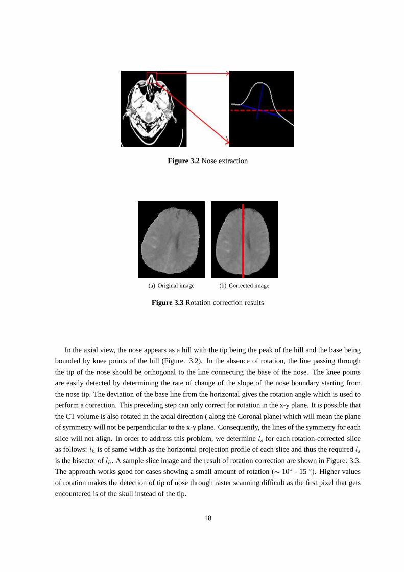
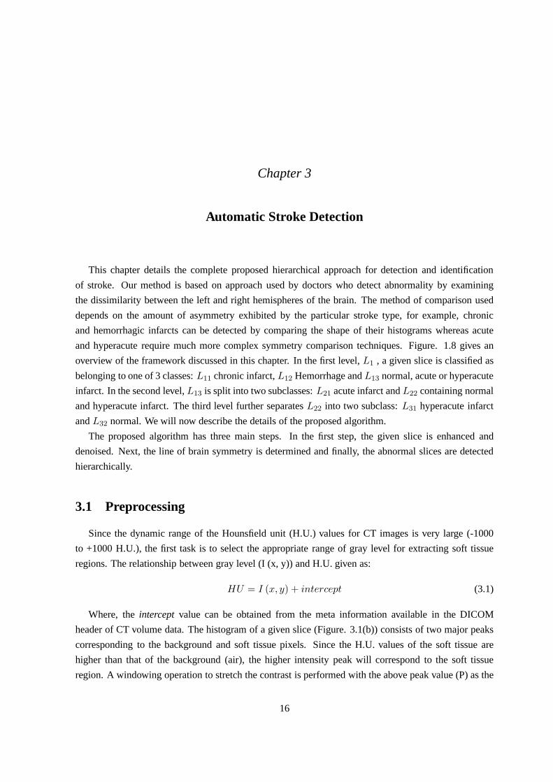
Figure 3.2Nose extraction

(a) Original image (b) Corrected image

Figure 3.3Rotation correction results

In the axial view, the nose appears as a hill with the tip beingthe peak of the hill and the base being

bounded by knee points of the hill (Figure. 3.2). In the absence of rotation, the line passing through

the tip of the nose should be orthogonal to the line connecting the base of the nose. The knee points

are easily detected by determining the rate of change of the slope of the nose boundary starting from

the nose tip. The deviation of the base line from the horizontal gives the rotation angle which is used to

perform a correction. This preceding step can only correct for rotation in the x-y plane. It is possible that

the CT volume is also rotated in the axial direction ( along the Coronal plane) which will mean the plane

of symmetry will not be perpendicular to the x-y plane. Consequently, the lines of the symmetry for each

slice will not align. In order to address this problem, we determinels for each rotation-corrected slice

as follows:lh is of same width as the horizontal projection profile of each slice and thus the requiredlsis the bisector oflh. A sample slice image and the result of rotation correction are shown in Figure. 3.3.

The approach works good for cases showing a small amount of rotation (∼ 10 - 15 ). Higher values

of rotation makes the detection of tip of nose through rasterscanning difficult as the first pixel that gets

encountered is of the skull instead of the tip.

18

(a) Chronic affectedhistogram

(b) Corresponding normalhistogram

(c) Hemorrhage affected his-togram

(d) Corresponding normalhistogram

Figure 3.4Histograms obtained at level 1

3.3 Stroke Detection and Identification

The detection algorithm performs a 3-level classification to identify abnormal and normal slices.

Histogram features are used in the first level while wavelet-based features are used for the second level.

In the third level, due to subtle nature of hyperacute infarct, rough gray/ white matter segmentation is

performed using Markov Random Field (MRF) and then their distributions in the two hemispheres are

compared spatially. The following sections describe each level of the framework in detail.

3.3.1 Level 1 Classification

The first step differentiates the encephalic slices into three classesL11, L12 andL13 as described

earlier, based on their histogram features. Thels information is used to divide a slice into two hemi-

spheres and the histogram for the right and left hemispheresare computed and compared for similarity.

The similarity metric used is the correlation coefficient which is computed on a subsampled (by 5) ver-

sion of the 2 histograms. The histograms of left and right hemispheres exhibit significant difference

in the lower intensity bins (50-100) in case of chronic infarct whereas for hemorrhage the difference is

observed in higher intensity bins (200-250) (Figure. 3.4).Since only the low and high indexed bins

are of interest, the measure is computed only for those bins.If this measure is below a threshold the

corresponding bin number is noted. If the bin number is low, the slice is classified as belonging toL11

and if the bin number is high the slice is classified as a memberof L12. If the measure is below the

threshold in both low and high indexed bins, the implicationis that both type of abnormalities present in

the slice. Therefore such slices are accorded membership inbothL11 andL12. All the remaining slices

are classified as belonging toL13.

3.3.2 Level 2 Classification

In the second level of classification, the goal is to differentiate between normal and acute infarct

cases. Histogram features are insufficient for this purposeas their gray value distributions overlap. This

19

(a) Acute infarct affectedhistogram

(b) Corresponding normalhistogram

Figure 3.5Histograms acute infarct

can be seen from the histograms shown in Figure. 3.5. Since the difference between the distributions

is subtle, a finer analysis is required. A wavelet decomposition of the histograms is employed for this

analysis. Daubechies-4 wavelet decomposition up to 5 levels is used to compute the energy distribution

in the scale space. The corresponding energy values of the two histograms are compared using a simple

difference of energy measure. If the difference is above a threshold, the slice is classified as belonging

toL21. All other cases are classified as normal (L21).

3.3.3 Level 3 Classification

The third level classification deals with the detection of hyperacute infarct. During the time frame of

hyperacute infarct (0-4 hrs.), very subtle changes occur inthe affected tissues. These include blurring

of gray/ white matter junction, hyperattenuation of blood vessels, edema related abnormalities etc. All

these indicators affect the distribution of gray/ white matter in the left and right hemispheres, but accu-

rate separation of brain tissues into gray/ white matter is very difficult owing to the poor tissue contrast

and noise offered by the CT images. As a result most of the tissue classification methods require some

sort of additional knowledge in the form of different modality images, etc. An example is [48] which

uses multimodal information from PET/CT pairs to boost the classification. In order to overcome these

limitations, we propose to a novel approach that uses rough segmentation of brain tissues. The aim of

the approach is to achieve a best possible segmentation of gray/ white matter and then use a symmetry

measure which negates the inaccuracies in the tissue segmentation.

Although work on tissue classification in CT is limited, it isa widely researched problem in brain

Magnetic Resonance (MR) images. Most of these methods employ probabilistic models ([30], [10],

[49] etc.) for tissue classification as these models providean effective way of incorporating spatial

information and are generally resistant to noise. In our method, we propose an automatic segmentation

of brain CT images by using MAP-MRF model [14] which combinesthe Markov random field (MRF)

and the maximum a posteriori (MAP) approach for classification. Such an approach has been adopted

20

(a) Gray/ white matter on Atlas (b) Gray/ white matter on CT

(c) Rough segmentation

Figure 3.6Rough segmentation of gray white matter on CT

for PET/ CT pairs [48] but not for CT exclusively. The next section explains the representation of a CT

image using MRF model.

MRF Model

We assume that images are defined over a finite lattice S =Si, 1≤i≤N where Si denotes the pixels.

The notation Si and subscript i are interchangebly used to demontrate the same location Si. For each

pixel S, the class to which the pixel belongs is specified by a class label, Li, which is modeled as a

discrete random variable L =Li, 1≤Li ≤M. We are also given an MRF on these units, defined by

a graph G (where the vertices represent the units, and the edges represent the label constraints of the

neighboring units), and the clique potentials. Let c denotea clique of G andΩ the set of all cliques of

G.

In MRF theory, a configuration refers to a state where each site Si belongs to a particular label Li.

Our goal is to find the best possible configuration L (L∈ ΨL, whereΨL represents the configuration

space), which maximizes the posterior probability of L. Theposterior probability is given by

P (L|S) ∝ P (S|L)P (L) (3.3)

21

Imposing an identical, independent Gaussian distributionfor the voxel values at each targeted region in

the given image, we have

P (S|L) =∏

1≤i≤N

P (Si|L) =∏

1≤i≤N

P (Si|Li) (3.4)

and,

P (Si|Li) =1√

2πσLi

exp

(

(Si − µLi)2

2σ2Li

)

(3.5)

whereµLiis the mean andσLi

, is the standard deviation of classLi. The prior model, P(L) can be

assumed to follow Gibbs distribution [16] given by,

P (L) =

∏

c∈Ω exp (−Ec)

Z(3.6)

WhereEc refers to the energy of the configuration andZ is a normalization factor. Combining equations

3.3, 3.4 and 3.6, we have for the posterior probability,

P (L|S) ∝∏

1≤i≤N

P (Si|Li)∏

c∈Ω

exp (−Ec) (3.7)

It is further assumed that the configuration field L is a secondorder MRF [22] which gives the prior

model as (using equation. 3.6),

P (L) =1

Zexp

−1

T

∑

Si,Sj∈Ω

βV(

LSi, LSj

)

(3.8)

Where T is the temperature,Ω is the set of second order cliques,β is a model parameter controlling the

homogeneity of regions and V(LSi, LSj

) represents the second order clique potential, defined as

V (LSi, LSj

) =

1, if LSi6= LSj

−1, otherwise(3.9)

The estimate of L denoted byL, global energy, (Eglob(L)) and the local energy (Ei(L) at site Si), are

determined following the method in [3]:

L = argminL∈Ψ

(

∑

1≤i≤N

(F (i))

+1

T

∑

Si,Sj∈Ω

βV(

LSi, LSj

)

(3.10)

22

Eglob(L) =

(

∑

1≤i≤N

(F (i))+

1

T

∑

Si,Sj∈Ω

βV(

LSi, LSj

)

(3.11)

The local energy at site Si is the energy of the site in isolation, given byF (i) and the energy of the

neighbourhood (Ωi) cliques.

Ei(L) = F (i)+

1

T

∑

Sj ,Sk∈Ωi

βV(

LSj, LSk

)

(3.12)

Where F(i) represents,

F (i) =1

T

(

log√2πσLi

+(Si − µLi

)2

2σ2Li

)

(3.13)

The segmentation process which minimizes the above mentioned energy requires the initialization of

the distribution parameters (mean, variance) of all the label classes. These parameters can be estimated

using various methods such as histogram analysis, maximum likelihood estimation, thresholding etc.

Since the estimation of distribution parameters influence the performance of the segmentation algorithm,

we want to partition the pixels into classes such that the interclass variability is maximum which is

achievable using Otsu’s method of segmentation [28]. We perform Otsu segmentation to classify the

brain pixels into M (=2) classes namely, white and gray matter. We need only two classes as after the

preprocessing only the soft tissues are left. Once the classes are determined, the distribution parameters

namely, mean and variance are calculated and provided to theenergy minimization algorithms for further

estimation.

The poor tissue contrast in CT will weigh down the performance of the segmentation algorithm. We

seek to address this by increasing the contrast between the various tissue classesprior to their segmen-

tation. The pipeline of processing for our proposed method is shown in Figure. 3.7. As indicated, the

processing is carried out at the slice level in the first two stages as well as in the probability map gen-

eration step. Midline detection and the final decision on thepresence of infarct are done at the volume

level. The complete pipeline is described in detail next.

3.3.3.1 Contrast Enhancement

Since only soft tissues are of interest, the first step is to extract the brain tissues which lie in the range

of white/gray matter (16-50 H.U) which results in strippingof skull, etc which lie outside the tissue

23

Figure 3.7Algorithm outline

range. These tissues are then enhanced using a method very similar to [7]. A CT slice is decomposed

into four frequency sub-bands using Daubechies9 wavelet to extract the illumination information of

the image. The illumination sub-band is then equalized, based on the intensity profile of the same

slice with modified window settings using singular value decomposition (SVD). The singular value

matrix obtained after SVD contains only the illumination information and hence modifying it results in

preserving other important details (Figure. 3.8(a)).

3.3.3.2 Tissue Segmentation

The tissue segmentation involves maximization of the posterior probability of the MRF model which

we calculated in the previous section. This is done using Modified Metropolis Dynamics (MMD) as it is

generally faster and provides a lower energy output when compared with other optimization techniques

[3]. MMD involves the following steps:

1. Pick up randomly an initial configuration L0, with iteration k=0 and temperature T=Ta (whereTa

is a constant).

2. Pick a global state L’ such that: 1≤L’ i ≤M and L’i 6= Lki, 1≤i≤N, Where k refers to the iteration

number.

3. For each site Si, the local energy Ei(L’), where L’ = (Lk1,. . .,Lk

i,. . .,LkN ) is computed using

equation 3.12.

24

4. Compute ∆Ei = Ei(L’) - E i(Lk), the new label at site Si is accepted if

if ∆Ei ≤ 0 or α ≤ exp(

−∆Ei

T

)

whereα ∈ (0,1) is a constant.

5. Decrease the temperature T (k+1) = a× T (k) (where a = 0.9 is a predefined constant, used to

control T andT (0)=4) and go to step 2 until the number of modified sites is less than a threshold.

To aid convergence of the algorithm, the entire image is firstpartitioned into disjoint regions Rn(1≤n≤2). This initial segmentation is carried out by assigning a label to each pixel which generates the

least amount of Gaussian energy (using log of equation 3.5).The tissue segmentation results in a binary

map with white matter indicated in black (Fig. 3.8(b)).

(a) Enhanced image (afterskull stripping)

(b) Extracted binary image

Figure 3.8Extraction of hypodense pixels.

3.3.3.3 Candidate Selection

Candidate affected pixels are identified based on contra-lateral symmetry of a slice. The left and right

hemispheres of a brain appear symmetric but are similar at best. Many small discrepancies exist even

in the normal brain [47] which can unfavorably affect any attempt to detect abnormality (like stroke)

based on global contra-lateral symmetry. These discrepancies, unlike stroke, seldom continue across the

slices (in axial direction) due to considerable thickness of the slices. Hence, the symmetry is assessed

in a 3-dimensional neighborhood (which is an × n× 3 (slices) window, W) of every hypodense pixel

in both the hemispheres and an abnormality measure P (-1≤ p ≤ 1) is defined as follows.

PSi=

∑

WSiRight

SiRight −∑

WSiLeft

SiLeft

3× n2(3.14)

Where, SiRight and SiLeft refer to corresponding pixel locations. Deviation of P from0 (symmetry

state) gives the measure of asymmetry in the distribution ofhypodense tissues in the vicinity of the con-

cerned tissue and its counterpart in the other hemisphere. Any deviation from the symmetry state (’0’)

implies excess of hypodense pixels thereby indicating higher possibility of infarct. The value|PSi|, is

25

Dicom Tag Information Value0008-0070 Manufacturer Siemens0008-1090 Model Name Emotion 60018-0050 Slice Thickness 6 mm0018-1150 Exposure Time 10000018-1151 X Ray Tube Current 240µA0018-5100 Patient Position HFS

Table 3.1CT acquisition protocol

the probability thatSi belongs to an infarct region. A higher value ofPSiindicates greater discrepan-

cies between the hemispheres atSi and thus exhibiting higher probability of presence of infarction. The

required candidates are found by applying a confidence threshold (determined empirically) to this map

in order to account for the natural asymmetry present in the brain.

3.3.3.4 Hyperacute Infarct Region Detection

Given the set of infarct candidates, we impose spatial contiguity across slices to reject the false can-

didates. This is achieved by declaring only those regions which show significant overlap in neighboring

slices as belonging to infarcts. The constraint helps in filtering out false positives which are detected by

the algorithm as they exhibit a natural asymmetry in tissue distribution.

3.4 Results and Discussion

3.4.1 Dataset Details

The performance of the method has been tested on a dataset collected from a local hospital. A

detailed acquisition protocol is given in Table. 3.1. The dataset consists of volume CT data of 42

patients. Out of these 19 were normal, 5 hemorrhagic, 6 chronic, 6 acute and 6 hyperacute. Since the

time of scan was not available, the abnormal cases were classified into chronic, acute and hyperacute by

the doctors based on the difficulty encountered while identifying the infarct regions. Follow up scans of

these cases were collected and one expert’s markings on these scans were used as the ground truth. The

scans were from patients belonging to various age groups (7,15, 20 datasets in the age-groups 0-30,

30-50, 50 and above respectively) to help in robust testing since natural symmetry is disturbed as the

age advances. In abnormal cases, it was assumed that the number of affected slices remained the same

in follow-up scans (i.e. no growth of abnormal tissue between subsequent scans).

26

Normal Cases Abnormal Stroke CasesPatients 19 23

InfarctHemorrhage

Chronic Acute HyperacuteSlices (Groundtruth) 291 40 61 45 35

True positive 261 38 56 37 28False negatives 30 2 5 8 7False positive 22 4 8 16 2

Recall(%) 89.69 95.00 91.80 82.22 80Precision(%) 92.22 90.47 87.5 69.81 93.3

Table 3.2Results of the complete system at slice level

3.4.2 Detection Results and Discussion

The qualitative results of the algorithm are showcased in Figure. 3.9 and 3.10. Figure. 3.9 show the

results of the MRF-based detection on a normal, acute and hyperacute dataset. The algorithm succeeds

in picking out the affected regions but in the process it alsopicks up false positives (Figure. 3.9(d)).

The reason being that the slice exhibits difference in tissue distribution in the lower side of brain which

can be easily seen from the extracted tissue map (Figure. 3.9(c)). Such differences in distribution occur

frequently in brain but fortunately the spatial contiguityconstraint takes care of most of them. Figure.

3.10 shows the outcome of detection algorithm on two more hyperacute slices side-by-side with their

corresponding follow-up CT scans. We can clearly see that the algorithm performs good as far as the

detection of core area of infarct is concerned, however it fails to detect the periphery regions of infarct

core as the symmetry disturbance in those region is not significant enough at the time of CT scan.

As discussed earlier, the detection of early infarct carries clinical value whereas the latter stages

of stroke carry mostly an academic importance. This makes itnecessary to present the results of our

algorithm under both clinical and academic requirements. We therefore, showcase the results of the

entire system as a whole, on the previously mentioned dataset (Table. 3.2) and also on a subset dataset

(Table. 3.3) comprising only hemorrhage, hyperacute and normal cases. We also include the acute cases

in this dataset as there is a fuzzy boundary between the hyperacute and the acute cases and it’s very

difficult to differentiate one from another. The performance on second dataset gives us a clearer picture

about the performance of the algorithm under clinical conditions. Moreover, to gauge the performance

of the entire approach with regards to separating normal andstroke (hemorrhage and ischemic) cases,

we present the corresponding performance figures for the same in Table. 3.5 . Apart from the slice level

results, we also present the patient level results (Table. 3.4) which gives true picture of the performance

of the algorithm. Patient-level results give us additionalinformation like number of affected patients

that were declared normal, also the number of normal patients which were declared as affected. The

27

former information is more important in case of medical imaging as the algorithm must ensure low false

negative rate even at the cost of a relatively high false positive rate.

Figure 3.9Results of proposed algorithm on normal, hyperacute and acute datasets (rows 1-3 resp.).Thecolumns 1-4 depict input image, enhanced tissue region, extracted hypodense tissue and detected abnor-mality (overlapped on input image) resp.

Table. 3.2 shows the performance of the algorithm at slice level. The algorithm performs well in

cases of chronic and acute infarct as is evident from the highprecision and recall figures. The presence

of a number of false negatives in these cases (2, 5 respectively) were mostly the boundary slices of the

infarct where only a fraction of infarct is present and the disturbance in contra-lateral symmetry is not

sufficient for detection. Figure. 3.11 shows the boundary slice of a stroke affected patient alongside a

similar slice from a normal patient. As is clear from the figure, the tissue distribution in both the slices

appear similar which causes the algorithm to miss the affected slice. Hyper acute detection figures are

slightly lower than chronic and acute cases, with precisionand recall rate being 69.81% and 82.22%.

In spite of the lower precision rate, a higher recall rate showcases the efficiency of the algorithm under

clinical conditions. The lower precision rate is mainly dueto the slices in which the inherent symmetry

of the normal brain is lost due to various reasons, for example, widening of sulci which can be seen in

28

Figure 3.10Results of proposed algorithm on hyperacute slices showinginput image, enhanced tissueregion, detected abnormal tissues, corresponding follow-up scan (in columns 1-4 respectively).

Normal Infarct HemorrhagePatients 19 12 5Slices 291 106 35

True Positive 261 93 28False Negative 30 13 7False Positive 20 28 2

Recall TP/(TP+FN) 89.69 87.73 80Precision TP/(TP+FP) 92.88 76.85 93.33

Table 3.3Results depicting clinical scenario

Figure. 3.11(b). Also, thicker slice reconstruction can result in partial volume effect which sometimes

mimics the hypodensity observed in ischemic stroke and can be falsely picked up by the algorithm. Also

a number of hyper acute infarct slices were missed by the algorithm, most of which were the boundary

slices exhibiting the same problems as explained before. Insome of the cases, the infarct might not

have reached the particular boundary slices when the initial scan was conducted. Since we assume in

the beginning that the number of affected slices remain the same between the initial and the follow-

up scan. Since in our case, most of the follow ups were taken around 1-2 days after the initial scan,

there is a possibility of growth of ischemic tissues due to complete infarction of the penumbra regions

[13]. Therefore due to lack of sufficient condition we still consider missed slices when compared to

follow up scans as false negatives which probably bring downthe actual performance of the algorithm

slightly. The algorithm also performs reasonably well in case of hemorrhage giving about 80% recall

and 93.33% precision. The higher precision value is mainly due to the contrast in the gray values of

hemorrhage (hyperdense) and normal brain tissues. Although, even in case of hemorrhage, various

mural vascular calcifications can mimic hyperdense regionsdue to partial volume effect and in some

cases are picked up by the algorithm as belonging to hemorrhage.

29

(a) Missed hyperacute slice (b) Normal slice

Figure 3.11Comparison of missed hyperacute boundary slice with normalslice

Table. 3.3 showcases the performance of the algorithm on a subset of the original dataset comprising

only of cases which have clinical importance i.e. hemorrhage, acute and hyperacute cases. In order to

be useful in clinical scenario, the algorithm must first be able to separate the hemorrhage cases from

the normal and hyperacute ones and then must be able to detectthe hyperacute cases with high degree

of accuracy. Our algorithm gives a recall rate of 80% and 87.73% in case of hemorrhage and early

infarct (both acute and hyperacute) cases respectively. The recall rate of hemorrhage detection seems

low indicating the shortcoming of the algorithm. The same istrue of infarct detection but to a lesser

degree. In spite of the lower performance, the numbers that really matter in clinical scenarios are the

patient level results which show the actual number of affected patients that go through undetected by

the system.

Normal Cases Abnormal Stroke CasesPatients 19 23

Patients (Groundtruth)Infarct

HemorrhageChronic Acute HyperAcute

19 6 6 6 5True positive 18 6 6 5 5

False negatives 1 0 0 1 0False positive 1 0 0 1 0

Recall (%) 94.73 100 100 83.33 100Precision (%) 94.73 100 100 83.33 100

Table 3.4Patient level results of the complete system

The patient level figures are shown in Table. 3.4. The figures indicate that even though the algorithm

is not able to pick out all the affected slices, it does pick out a few in each affected case to mark them

as affected. The algorithm gives 100% precision and recall in case of chronic, acute and hemorrhage.

The slightly lower performance in case of hyperacute was dueto inability of the algorithm to detect any

stroke slice in a hyperacute case having a small infarct visible in just two slices. The presence of infarct

30

(a) Slice 1 (b) Slice 2

Figure 3.12Hyperacute failure case (infarct indicated by arrow)

Normal Stroke-affectedPatients 19 23Slices 291 181

True Positives 261 157False Negatives 30 24False Positives 22 30

Recall (%) 89.69 86.74Precision (%) 92.22 83.95

Table 3.5Table showing system level performance

in just two slices mimics the behavior of the typical asymmetry shown by the abnormal CSF distribution

by the normal brain and is therefore classed as same. Figure.3.12 shows the above referred case.

Finally, in Table. 3.5, we present the slice level results togauge the performance of the system in

a normal vs. stroke-affected (both ischemic and hemorrhagic stroke) scenario. In this scenario, our

approach registered a high recall and precision rate (86.74% and 83.95% respectively) for detection

of stroke on brain CT. The above tabulated results indicate areasonable level of performance in case

of hyperacute stroke which carries the maximum clinical importance. This encouraged us to look for

alternate approaches for increasing the accuracy of radiologists in detecting early infarcts. The next

chapter describes one such approach which aims at empowering the radiologists with more information

to make their decision making as accurate as possible.

31

Chapter 4

Enhancement of Early Infarct through Auto-Windowing

As explained in previous chapter, automatic detection of hyperacute infarct from non-contrast CT

is a very difficult task mainly because of the subtle developments which take place in the affected

region which are often masked by the low tissue contrast and the noisy nature of CT scans. Clinically,

detection of hyperacute infarct is of utmost importance andsince the automatic detection rates were low,

a different strategy was adopted to increase the accuracy ofradiologist for hyperacute infarct detection.

The new strategy was inspired by the current detection method adopted by the radiologists in case

of hyperacute infarcts and focuses on enhancement of infarct tissues rather than its automatic detection.

The enhancement strategy can help the radiologists in clinical scenarios by making the infarct tissue

easier to detect. The doctors currently use a manual windowing procedure to look for the various signs

exhibited by the infarct tissues during the early hours of onset. In the coming sections we will first

describe the windowing process before moving onto our automatic approach.

4.1 Manual Windowing

CT scans produce 16-bit images consisting of 65, 536 different grayscale values. Only a small por-

tion of these grayscale values contain information useful for the radiologists, with the rest representing

the attenuation coefficients of air, surrounding objects, etc. Windowing in medical images refers to

selecting the required range of grayscale values out of the 65, 536 and mapping them to the display

range of the monitor. Different chunks of grayscale values provide different information about the scan

and windowing can help in looking at various different aspects of the CT like bones, soft tissue, etc. in

isolation. Figure 4.1 gives a good idea of the windowing process.

Mathematically, Windowing is defined as a one to one mapping function between two sets of inten-

sities, source intensities (Ls ∈ Ls1, Ls2, ..., Lsm) and the destination display intensities (Ld ∈ Ld1,

Ld2, ...,Ldn). In case of medical imaging, the destination is the displaymonitor having intensity range

Ld ∈ (0, 1, 2, ..., 255). The range of source intensities is described in terms of twoparameters, window

width Wwidth and window centerWcenter such that,

32

(a) Histogram of a normal slice

(b) Entire CT range (c) Soft tissue range (d) Hard tissue range (bone)

Figure 4.1Demonstration of windowing process

33

(a)

Figure 4.2Representation of contrast stretching/ compressing (windowing)

Ls1 = Wcenter −Wcenter

2(4.1)

Lsm = Wcenter +Wcenter

2(4.2)

The mathematical equation representing windowing can be written as,

Ld =

(

Ls −Wcenter −Wcenter

2

)

×(

255 − 0

Wwidth

)

(4.3)

Where,Ld andLs represent the source and destination grayscale values respectively. Windowing

also performs contrast stretching/ compression based on the values of m and n. Contrast stretching

occurs when the range of grayscale values (m) selected to be displayed is smaller than that of the display

monitor (n) and vice versa (Figure. 4.2). The shorter the span of grayscale values to be mapped, the

higher the contrast enhancement achieved. The enhancementbetween the various tissue types helps the

radiologists to identify subtle discrepancies in the tissues which were earlier very difficult to detect.

The radiologists use the windowed CT scans to detect any signs of early infarct. The most important

sign of infarction is the loss of gray/ white matter interface which can be really difficult to spot when

windowed at the entire soft tissue range (std. settings) butwhen viewed under appropriate (reduced)

window settings, become relatively easier to detect. The shortening of the window width decreases the

amount of tissues lying in the window range. Therefore, in order to look for the tissue discrepancies

across the entire tissue range, the doctors must manually slide the window to cover the entire intensity

34

(a) Stroke standard win-dow

(b) (Window Center -1050, Width - 25)

(c) (1055, 25) (d) (1060, 25)

(e) (1050, 40) (f) (1055, 40) (g) (1060, 40)

Figure 4.3Stroke appearance under reduced window settings (center, width).

range. The selection of appropriate window width and centerresembles a trial and error process whose

accuracy depends on the experience of the radiologists [50]. The main reason for experience playing

such a large role in window selection is that windowing, while achieving contrast enhancement also

tends to increase the noise and artifacts in the scan. All these factors compounded by the poor tissue

contrast offered by the CT may adversely affect the judgmentof doctors. With increased experience and

training, the doctors learn to distinguish between the trueischemic signs and the artifacts. Figure. 4.3

shows the appearance of an early infarct scan under different window settings. Moreover, Krupinski et

al. [18] mentions the effect of workload and fatigue on the detection accuracy of the radiologists which

may result in missed infarct cases. Although the study presents the case of fracture detection, a similar

observation may also be derived for hyperacute infarct where the affected tissue mimic the property

of normal tissues and require higher concentration levels to detect amid all the noise and artifacts.

Automatic enhancement of affected tissue will therefore goa long way in minimizing all these risks.

As discussed in chapter. 2, a lot of research has gone into finding an appropriate contrast enhance-

ment. Although non-linear enhancements increase the contrast between the normal and abnormal tissue

appreciably, they also tend to introduce unwanted artifacts and noise [20]. These can adversely influence

the decision making of the radiologists. One way of countering the errors can be through increasing fa-

miliarity with the concerned method but making it a standardlike the current prevalent windowing

process is too much of an ask. Therefore the best way to increase the detection rate of early infarct is

through automating the tried and tested windowing process currently used by radiologists.

The purpose of this study was to develop an algorithm to improve the diagnostic accuracy of early

infarct by maximizing perceptual contrast between normal and abnormal tissues using linear enhance-

ment of tissue intensities. We aim at minimizing the ’experience’ factor in the current detection process.

35

Figure 4.4Histograms ofVi andVic

In the coming sections, we present two different strategiesfor determining the optimal window settings

based on 1. Region-level and 2. Pixel-level properties of the brain CT. Both the tracks leverage the

asymmetrical subtle changes that occur during the early times by emphasizing them and thus help dis-

tinguish between normal and abnormal (stroke affected) tissue. These strategies although being stroke

specific, can also be applied to accentuate the differences in similar other abnormalities of the tissues.

4.2 Region Based Windowing

The region based method takes off from where the hyperacute detection method stopped in chapter. 3.

At the end of the detection process, we are left with stroke affected tissues. The required window settings

are then determined as follows. Given a detected infarct volumeVi, its counterpart volumeVic is first

extracted from the other hemisphere. Assuming this represents a normal volume, maximum perceptual

contrast between the normal and affected tissue regions is achieved by setting the window center at a

point such that the distribution is balanced about this center. This is achieved by computing intensity

histograms ofVi andVic and finding the bin corresponding to the point of maximum overlap between

the histograms (Figure. 4.4). The window width can be chosenaccording to the tissue information

desired by the radiologist as the above window center will provide maximum contrast irrespective of

width. Figure. 4.5 shows the test images under modified window settings (window width is taken as 25

H.U.). In the next section, we present a different approach to windowing using the pixel level properties.

4.3 Pixel Based Windowing

Pixel-based windowing is a novel approach inspired by ideasof binary image thresholding. In thresh-

olding, the aim is to divide the image pixels into two exclusive classes of intensities based on optimiza-

tion of a criterion function. In our method, we achieve best possible windowing for aiding stroke

detection by selecting an intensity range which maximizes the difference in distribution of pixels in left

and right hemispheres. Although the underlying principlesare the same, the proposed method differs

from thresholding as it chooses a single class of intensities based on two images whereas thresholding

36

Figure 4.5 Results of proposed algorithm on normal (row: 1 ) and hyperacute (row: 2).The columns1-3 depict input image, detected abnormality (overlapped on input image) and the original image undermodified viewing window settings respectively.

chooses two classes of intensities based on a single image. The window settings (center and level) are

then computed from the obtained intensity range.

Since the early days, a variety of approaches have been proposed for thresholding a gray scale image.

Some of the most widely used among them are Otsu, Minimum error thresholding, Entropy based

methods etc. All these methods have different strengths andweakness. A more detailed explanation

can be found in [37]. We base our windowing technique on a recently proposed thresholding approach

based on parzen-window estimate [46]. The main reason for selecting the above was the ease with

which the framework could be exploited to perform thresholding on a pair of images rather than on a

single image. Other factors which weighed favorably towards its selection were the incorporation of

spatial information of pixels apart from the better thresholding results compared to other commonly

used approaches. Incorporation of spatial information wasnecessary for detecting the disturbances in

the contra-lateral symmetry. In the coming sections, we first describe the theory behind parzen window

estimation and how it’s used in context of images.

4.3.0.1 Parzen Window

The parzen window based non-parametric density estimationapproach was first proposed by [35],

[29]. We first describe the parzen window concept when applied to images. Let I be an image of size m

x n having gray values from 1 to L. We define a pixel location as(x,y) : x ǫ (1,2,...,m), yǫ (1,2,...,n)and its value as f(x,y)ǫ (1,2,3,...,L). Letωi = (x,y) : f(x,y)=i andCi = |ωi| giving N, total number of

pixels as N =∑L

i=1Ci. The probability density functionP (x, y) at (x,y) can be estimated using parzen

window as

37

P(x,y)=L∑

i=1

P (x, y, ωi) =L∑

i=1

P (ωi)P (x, y|ωi) (4.4)

Where,

P (x, y|ωi) =1

Ci

Ci∑

j=1

1

VCi

K(

x, y;xj , yj ;hdCi

)

(4.5)

P (ωi) =Ci

N(4.6)

Where K (.) is called a kernel function,VCidenotes the volume of d-dimension hypercube having

edgehCi. Since we are dealing with 2 dimensions here, d is taken as 2 and VCi = h2Ci [9]. The kernel

function must be designed in a way that is inversely proportion to distance between (x, y) and (xj , yj)

so that farther pixels contribute less towards the density estimate and vice versa. In our approach we

take the kernel function to be a Gaussian. Most of the parzen density based approaches suggestVCi=

1/√Ci as a good estimate. Next, we will describe how the parzen window principle in incorporated in

our windowing approach.

K(

x, y;xj , yj ;h2Ci

)

=1√2π

exp

(

−(x− xj)2 + (y − yj)

2

2h2Ci

)

(4.7)

4.3.0.2 Parzen Based Windowing

As mentioned earlier, one of the earliest visible signs of acute infarct on CT includes the distur-

bance in the contralaterally similar distribution of whiteand gray matter. The idea is to exploit this

phenomenon to find the intensity range where this disturbance is most perceptible. LetWc andWw be

the target window center and width respectively. The present windowing procedure used by radiologists

takes the tissues which lie in the intensity rangeωw,c = [Wc - Ww/2, Wc+Ww/2] and c, wǫ[1, L] and

then stretches the intensity range to the visible intensityrange (0-255). Our approach aims at finding

the optimal intensity rangeωt based on a criterion function which maximizes the disturbance in left and

right hemisphere images. LetPl andPr denote the probability density function of pixels in left and right

hemispheres respectively, in the intensity rangeωw,c and can be estimated using parzen window as

Pl =∑

kǫωleft

Pl (xk, yk) =∑

kǫωleft

1

N

∑

iǫωw,c

Cil∑

j=1

1

VCil

K(

xk, yk;xj , yj ;h2Cil

)

(4.8)

Pr =∑

kǫωright

Pr (xk, yk) =∑

kǫωright

1

N

∑

iǫωw,c

Cir∑

j=1

1

VCir

K(

xk, yk;xj , yj ;h2Cir

)

(4.9)

Where,ωleft andωright are the set of pixels in left and right hemispherical image. Now we need

to determine a criterion function whose optimization will lead us to the optimal window settings. The

38

simplest mathematical function that ensures maximum difference in the probability distributions of left

and right hemispheres is|(Pl − Pr)|.

(width, center)optimum = argmaxw,c|(Pl − Pr)| (4.10)

The above criterion function is bi-variable in w, c and further increases the computational complex-

ity of the already computationally intensive parzen estimate. The criterion function, however, can be

reduced to a single variable form in the special case of brainby utilizing some domain knowledge. Ever

since the advent of soft copy of CT, much work has gone into finding the best possible predetermined

window parameters. These parameters, especially window width, ensure that noise and other artifacts

that get accentuated with the windowing process do not adversely affect the radiologist’s judgment. In

order to make sure our algorithm is immune to such damage, we limit the width parameter to the one

designated by the stroke protocol (10) and then use the criterion function to find best possible window

center. The complete algorithm is given below.

1. Threshold the given CT scan to obtain only the brain tissues and correct for rotation by finding

the mid-sagittal plane (Section. 3.2).

2. Divide the given image into left and right hemispheres using the mid-sagittal plane.

3. Next for each gray level in the image as window center, i, compute t(i) = |(Pl − Pr)| with the

intensity range as [i-10,i+10].

4. Choose the gray level, i*, such thatt(i∗) ≤ t(i) for all i 6= i∗.

5. Output the image with (i*,10) as window parameters (Figure. 4.6).

4.4 Results

4.4.1 Experiment Details

The windowing results obtained from Region-based (Wr) and Pixel-based (Wp) methods were com-

pared by means of perception study conducted in an clinical environment. The results from the two

automated methods were compared with each other as well as with the standard window settings (Ws,

width 80 H.U. and center 40 H.U.). A set of 15 slices was selected from each of the hyperacute and

normal dataset and each slice was presented randomly under the different window settingsWr, Wp and

Ws to the radiologists. Since the region-based method performs enhancement only in cases in which it

detects an infarct, all such slices from the above set (normal cases and missed infarct slices) were shown

to the users with the window settings as:Ws. The inclusion of infarct cases which were missed by the

region-based method gives us an opportunity to test the mainadvantage of pixel-based method over the

39

Figure 4.6Results of proposed parzen-based windowing algorithm on normal (row: 1 ) and hyperacute(row: 2).The columns 1-3 depict input image, original imageunder modified viewing window settingsobtained using parzen-based method and using region-levelmethod respectively.

Reader 1 2 3 4Setting Wp Wr Ws Wp Wr Ws Wp Wr Ws Wp Wr Ws

Sensitivity 100 93.3 73.3 93.3 80 66.6 73.3 73.3 53.3 73.3 73.3 46.6Specificity 100 100 93.3 100 100 86.6 100 100 80 93.3 93.3 73.3Accuracy 100 96.6 83.33 96.6 90 76.6 86.6 86.6 66.6 83.3 83.3 60

Table 4.1Clinical study results

region based method. In the current set of 15 abnormal slices, 2 of these slices were the ones having

infarct region missed by the region-based method. Each slice was rated by 4 radiologists, having varied

experience, in a blinded review for the presence of hyperacute infarct. Their response as well the time

taken for decision was recorded. In compliance with similarclinical studies, the statistical significance

of the results of the above experiment was also evaluated using two tailed student’s t-test.

4.4.2 Discussion

Table. 4.1 shows the results of the clinical study. The results showcases the superior performance of

both automated windowing methods (Wp, Wr) against the standard window setting. Average sensitiv-

ity showed statistically significant increase in the performance from 59.95% in case ofWs to 79.97%

40

and 84.97% in case ofWr andWp respectively. (P = 0.034 forWp, P = 0.040 forWr, two-tailed stu-

dents’ t test.) The average specificity numbers also showed arise from 83.3% (Ws) to 98.34% (Wr)

and 98.34% (Wp). As seen with sensitivity, the specificity numbers also showed statistical significance

in accordance with the students’ test (p = 0.032 forWr andWp). The overall accuracy of the radiol-

ogists (measured in terms of the percentage of slices correctly identified) which was only around 71%

underWs increased to 91.6% (Wp, p = 0.024) and 89.16% (Wr, p = 0.034) in case of the automated

methods. The above results showcase the increase in the performance of radiologists when viewing the

test scans under automatically determined window settings. Moreover, the higher sensitivity numbers

prove our earlier thoughts that the enhancement of test images are not achieved at the cost of specificity

which certainly seem to the happen in case of non-linear enhancement. Also, there was no case where

a correct identification of infarct underWs was reversed when observed underWp/Wr. The slight ad-

vantage in performance of pixel-based method is because of the presence of 2 stroke slices on which the

region-based enhancement fails to perform the appropriateenhancement. These slices were having very

small infarct which gets enhanced by the pixel-level methodand thus gets detected by the experienced

radiologists. Another thing to note is that the region basedmethod provides same window parameters

for the entire scan where as the pixel-level algorithm provides window parameters adapted to the distur-

bance in that particular slice. This way the pixel-level approach provides better enhancement of infarct

tissues present in the border slices where the tissues are generally less hypodense than in the core infarct

region.

The similarity in performance observed by both pixel and region-based methods is because both the

methods aim for exploiting essentially the same sign that points at the presence of infarct (blurring of

gray/ white matter junction). InWr, the algorithm first divides the brain tissues into gray/ white matter

regions before comparing the overlap whereas, inWp, the gray/ white matter are compared directly. The

difference being,Wr requires a threshold to separate normally observed asymmetry from the asymmetry

due to presence of stroke and hence in order to keep the false positives down, the algorithm misses cases

in which the gray/ white matter asymmetry caused due to stroke is very weak. Hence the algorithm

does not enhance these cases as they are classified as normal whereas the pixel-based method requires

no such threshold and always produce enhancement no matter how weak the stroke is. Although since

the pixel-level is local in nature, it does tend to get easilyeffected by the other small disturbances which

are also present in the normal brain e.g. slight aberration in CSF distribution. As a result, though both

the methods exploit the same early infarct signs, the enhancement achieved is slightly different mainly

because of the difference in the position of the window center. The window centers obtained by the

region-level method are generally more specific i.e. are more characteristic to the infarct region and also

are generally on the left side of those obtained by the pixel-level approach on the Hounsfield number

line. One probable disadvantage, from the algorithmic point of view is that both the windowing methods

are computationally very expensive.

41

Chapter 5

Conclusions

In this thesis we presented a unified framework for automaticdetection and classification of stroke

from brain CT scans for both diagnostic and academic purposes. We also proposed two different image

adaptive approaches for automatic enhancement of stroke affected tissues. In this chapter we will review

the approaches and also present future directions in which the approaches can be improved.

5.1 Automatic Detection

We presented a unified hierarchical approach for automatic detection and classification of all types

of stroke. Previously proposed approaches mostly relied onthe characteristics of stroke affected tissues

and thus cannot be applied across all types of stroke owing tolarge variation observed in the behavior of

affected tissues relative to the normal ones. We therefore exploit a common property exhibited by both

ischemic and hemorrhagic stroke. Our approach models the stroke as a disturbance in the otherwise

similar distribution of brain tissue with respect to the mid-sagittal plane (MSP). We designed an easy to

difficult perceptible method which identifies the most easily perceptible stroke at each hierarchical level

resulting in the identification of first hemorrhage, chronic, acute and finally the least perceptible hyper-

acute infarct. In order to correctly estimate the contra-lateral symmetry of brain tissues, we proposed a

new robust MSP detection algorithm based on the physical structure of the skull. The method benefits

from the fact that the physical structure unlike soft tissuesymmetry rarely change in the event of stroke

and thus can be used for more robust detection of MSP even in stroke affected patients. The first phase of

the algorithm aims at detection of hemorrhage and chronic infarct. The affected tissues in these appear

hyper- and hypodense respectively as compared to normal brain tissues. Since the affected tissues at this

level are easily perceptible, a subsampled histogram basedapproach was proposed for their detection.

The histogram comparison gives a broad idea of symmetry which gets disturbed only by the presence

of affected tissue and remains unaffected by the usually present asymmetry in the normal brain. Thus

the method works well in cases where an appreciable amount ofaffected tissue is present. Although the

amount of false negatives (missed stroke cases) can be decreased by setting a low threshold value for

histogram comparison, this might give rise to an increased number of false positives mainly due to the

42

irregularities in the CSF distribution across the MSP. In future, to detect the smaller stroke tissues, we

can go for a grid-based histogram comparison rather than comparing the entire histogram at the same

time. The approach can be designed in a broad to narrow scenario where the symmetry comparison

is done at several spatial levels (cell ->block ->grid) and then a final consolidated symmetry measure

is prepared. The symmetry comparison at lower spatial levelwill ensure that even smaller infarcts get

picked up. The false positive in this case can be eliminated using anatomical information about the CSF.

The next phase of the algorithm involves the detection of acute infarct. The acute infarct is less

perceptible than the hemorrhage and chronic stroke and thuscannot be detected by histogram detection.

We therefore propose a novel approach which exploits the fact that acute affected tissues contain more

water and thus perceptually appear more ‘settled’ owing to them being slightly less granular than the

normal tissues. We quantify this degree of ‘settledness’ based on the wavelet energy of the contra-lateral

hemispheres. The approach gives high detection success butsuffers from the same problem of being too

broader like the first phase of the algorithm.

The third and the most important phase (from diagnostic point of view) of the algorithm deals with

the detection of hyperacute infarct. The affected tissues at this stage mimic the properties of the white

matter and thus cannot be differentiated from the normal white matter tissues in the intensity plane. We

therefore perform the symmetry comparison on the spatial characteristics of the tissues which gives us

the regions exhibiting loss of gray/ white matter differentiation. In order to compare the spatial charac-

teristics, we proposed a novel idea of rough tissue segmentation which gives the broader arrangement of

gray/ white matter tissues. The spatial distribution of thegray/ white matter tissues are then compared

and a loss of symmetry is attributed to hyperacute stroke. The symmetry comparison is designed in

such a way that it negates the effect of the roughness in segmentation of gray/ white matter tissues. The

algorithm provides an appreciable recall rate but also reports a large number of false positives. As seen

with other two phases, the smaller or less perceptible infarcts may sometimes pass undetected through

the algorithm. A similar grid based approach in this case will probably not work in this case since the

degree of asymmetry exhibited by hyperacute stroke in the missed slices was almost similar to the one

exhibited by normal brain and will further increase the false positives.

5.2 Enhancement of Affected Tissue

Next, we proposed a novel auto-windowing approach to overcome the limitations observed by the

automatic detection approach. The non-standard window parameters were determined automatically to

ensure the maximum possible contrast between the normal andaffected tissues. The window param-

eters were derived using two different approaches. The firstapproach used region level properties to

determine the window parameters based on the intensity characteristics of the detected stroke regions in

the hyperacute detection step. The other approach exploitsthe pixel properties of the brain CT and finds

the window parameters which maximize the disturbance in tissue (pixel) distribution in the left and right

hemisphere. Both the methods showcased encouraging improvement in the detection accuracy of the

43

radiologists. Moreover the jump in performance was more in case of inexperienced radiologists as com-

pared to the experienced ones. The method presents a way to counteract the effects of experience and

loss in concentration due to fatigue etc. by automatically finding the best possible window settings. One

of the drawbacks of region level approach is its inability tofind the optimal window parameters when

the detection algorithm fails to detect the infarct. The pixel level approach leaves the decision making

to the radiologists and finds the parameters in every case. Although this ensures the enhancement of

even smaller infarcts, the method might get influenced by thenoise/artifacts in the image unlike the

region based method which tries to remove them based on decision making. In the future, the clinical

study conducted in chapter 4 can be done on a much larger scaleto test the relative strengths of each

algorithm. Also to gauge the real performance of the automatic windowing, the experiments must be

conducted with scans under radiologist-modified window settings rather than with standard window set-

tings as is the case in chapter 4. Even though the windowing algorithm was developed keeping in mind

its application for detection of early infarct on CT, it can be easily used in other pathology cases which

present similar challenges. A very recent study conducted by [43] came to a conclusion that in spite

of all the technological advances, stroke windows still continue to be a powerful tool in detection of a

number of brain pathologies and must be a critical part of allhead CT examination and not only limited

to brain stroke. This encouraged us to look for similar problems in brain. One such problem that was

looked at, was the early detection of brain tumor which lookssimilar to gray matter (hyperdense) in the

early stages of its development (Figure. 5.1). Initial enhancement results obtained using our windowing

approach are very encouraging and indicate a similar quality of enhancement being achieved in the case

of tumors as with the hyperacute infarct. Although a more thorough evaluation will be required in order

to gauge the performance in case of tumor analysis. Moreover, there is also a provision for extending

the windowing process to other parts of human body which exhibit some or other kind of contra-lateral

symmetry.

(a) Standard window set-tings

(b) Non standard win-dow settings

Figure 5.1Appearance of early tumor lesions on CT scan [43]

44

Related Publications

• ”A method for automatic detection and classification of stroke from brain CT images”, M. Chawla,

S. Sharma, J. Sivaswamy, Kishore L.T, International Conference of the IEEE Engineering in

Medicine and Biology Society, 2009

• ”Automatic Detection of Early Infarct from Brain CT”, S. Sharma, J. Sivaswamy, International

Symposium on Medical Imaging in conjunction with ICVGIP 2010.

• ”Assisting acute infarct detection from non-contrast CT using image adaptive window setting”,

S. Sharma, J. Sivaswamy, R. Power, L. T. Kishore, Medical Image Perception Conference, 2011.

45

Bibliography

[1] J. E. Barnes. Characteristics and control of contrast inCT. Radiographics, 12(4):825–837, 1992.

[2] M. Bendszus, H. Urbach, B. Meyer, R. Schulthei, and L. Solymosi. Improved CT diagnosis of acute mid-

dle cerebral artery territory infarcts with density-difference analysis.Neuroradiology, 39:127–131, 1997.

10.1007/s002340050379.

[3] M. Berthod, Z. Kato, S. Yu, and J. Zerubia. Bayesian imageclassification using markov random-fields.

Image and Vision Computing, 14(4):285–295, May 1996.

[4] T. Chan. Computer aided detection of small acute intracranial hemorrhage on computer tomography of

brain. Computerized Medical Imaging and Graphics, 4-5:285–298, July 2007.

[5] V. Choksi, D. J. Quint, P. Maly-Sundgren, and E. Hoeffner. Imaging of acute stroke.Applied Radiology,

34(2):10–19, 2005.

[6] D. Cosic and S. Loncaric. Computer system for quantitative analysis of ICH from CT head images.In

Proceedings of the 19th Annual Int’l Conference of the IEEE EMBS, 1997.

[7] H. Demirel, C. Ozcinar, and G. Anbarjafari. Satellite image contrast enhancement using discrete wavelet

transform and singular value decomposition.IEEE GRS Letters, 7(2):333 –337, April 2010.

[8] A. P. Dhawan, S. Loncaric, K. Hitt, J. Broderick, and T. Brott. Image analysis and 3-d visualization of

intracerebral brain hemorrhage.Proceedings of the Sixth Annual IEEE Symposium on Computer-Based

Medical Systems, pages 140–145, 1993.

[9] O. Duda, P. Hart, and D. Stork.Pattern Classification. USA: John Wiley and Sons, 2000.

[10] M. El-Melegy, Y. Hasan, and H. Mokhtar. MRI brain tissues segmentation using non-parametric technique.

pages 185 –190. ICCES 2008, 25-27 2008.

[11] L. M. Fayad, Y. Jin, A. F. Laine, Y. M. Berkmen, G. D. Pearson, B. Freedman, and R. Van Heertum. Chest

CT window settings with multiscale adaptive histogram equalization: Pilot study.Radiology, 223(3):845–

852, 2002.

[12] J. Fiebach, P. Schellinger, O. Jansen, M. Meyer, P. Wilde, J. Bender, P. Schramm, E. Jttler, J. Oehler,

M. Hartmann, S. Hhnel, M. Knauth, W. Hacke, and K. Sartor. CT and diffusion-weighted MR imaging in

randomized order.Stroke, 33(9):2206–2210, 2002.

[13] M. Fisher and M. Ginsberg. Current concepts of the ischemic penumbra: Introduction.Stroke, 35:2657–

2658, 2004.

46

[14] S. Geman and D. Geman. Stochastic relaxation, gibbs distributions, and the bayesian restoration of images.

PAMI, PAMI-6(6):721 –741, nov. 1984.

[15] J. M. Gomori and I. Steiner. Non-linear CT windows.Computerized Radiology, 11(1):21 – 27, 1987.

[16] J. M. Hammersley and P. Clifford. Markov field on finite graphs and lattices. 1971.

[17] E. Hudyma and G. Terlikowski. Computer-aided detecting of early strokes and its evaluation on the base of

CT images. pages 251–254. IMCSIT 2008, Oct. 2008.

[18] E. A. Krupinski, K. S. Berbaum, R. T. Caldwell, K. M. Schartz, and J. Kim. Long radiology workdays

reduce detection and accommodation accuracy.Journal of the American College of Radiology, 7:698–704,

2010.

[19] Y. Lee, N. Takahashi, D.-Y. Tsai, and K. Ishii. Adaptivepartial median filter for early CT signs of acute

cerebral infarction.IJCARS, 2:2:105–115, June 2007.

[20] J. L. Lehr and P. Capek. Histogram equalization of CT images.Radiology, 154(1):163–169, 1985.

[21] M. H. Lev, J. Farkas, J. J. Gemmete, S. T. Hossain, G. J. Hunter, W. J. Koroshetz, and R. G. Gonzalez.

Acute stroke: Improved nonenhanced CT detection: Benefits of soft-copy interpretation by using variable

window width and center level settings.Radiology, 213(1):150–155, 1999.

[22] S. Z. Li. Modeling image analysis problems using markovrandom fields. volume 21 ofHandbook of

Statistics, chapter 13, pages 473 – 513. Elsevier, 2003.

[23] Y. Li, Q. Hu, J. Wu, and Z. Chen. A hybrid approach to detection of brain hemorrhage candidates from

clinical head CT scans.Sixth International Conference on Fuzzy Systems and Knowledge Discovery, 2009.

[24] R. Liu, C. L. Tan, T. Y. Leong, C. K. Lee, B. C. Pang, C. Lim,Q. Tian, S. Tang, and Z. Zhang. Hemorrhage

slices detection in brain CT images.International Conference on Pattern Recognition, pages 1–4, December

2008.

[25] Z. Majcenic and S. Loncaric. CT image labeling using simulated annealing algorithm.IX European Signal

Processing Conference, Island of Rhodos, Greece, 1998.

[26] J. A. Maldjian, J. Chalela, S. E. Kasner, D. Liebeskind,and J. A. Detre. Automated CT segmentation and

analysis for acute middle cerebral artery stroke.AJNR, American Journal of Neuroradiology, 22(6):1050–

1055, 2001.

[27] M. Matesin, S. Loncaric, and D. Petravic. A rule-based approach to stoke lesion analysis from CT brain

images.Proceedings of the 2nd International Symposium on Image andSignal Processing and Analysis,

2001.

[28] N. Otsu. A threshold selection method from gray-level histograms.TSMC, 9(1):62–66, jan. 1979.

[29] E. Parzen. On estimation of a probability density function and mode.Annals Math. Statist., pages 1065–

1076, 1962.

[30] Z. Peng, W. Wee, and J.-H. Lee. MR brain imaging segmentation based on spatial gaussian mixture model

and markov random field. volume 1, pages I – 313–16. ICIP, 11-14 2005.

47

[31] N. Perez, J. Valdes, M. Guevara, and A. Silva. Spontaneous intracerebral hemorrhage image analysis meth-

ods: A survey.Advances in Computational Vision and Medical Image Processing, pages 235–251, 2009.

[32] J. M. Provenzale, R. Jahan, T. P. Naidich, and A. J. Fox. Assessment of the patient with hyperacute stroke:

Imaging and therapy.Radiology, 229(2):347–359, 2003.

[33] A. Przelaskowski, K. Sklinda, P. Bargieł, J. Walecki, M. Biesiadko-Matuszewska, and M. Kazubek. Im-

proved early stroke detection: Wavelet-based perception enhancement of computerized tomography exams.

Comput. Biol. Med., 37(4):524–533, 2007.

[34] A. Przelaskowski, J. Walecki, K. Szerewicz, and P. Bargiel. Acute stroke detection in unenhanced CT

exams: perception enhancement by multi-scale approach. pages 94–95. Proceedings of National Conference

on Physics and Engineering in the Present Medicine and Health Care, 2005.

[35] M. Rosenblatt. Remarks on some non parametric estimates of a density function.Annals Math. Statist.,

pages 832–837, 1956.

[36] J. L. Saver. Time is brain–quantified.Stroke, 37(1):263–266, 2006.

[37] M. Sezgin and B. Sankur. Survey over image thresholdingtechniques and quantitative performance evalu-

ation. Journal of Electronic Imaging, 13(1):146–168, 2004.

[38] H. Simon. Gray and white matter of the brain. [Online], June 2008.

[39] K. Sklinda, P. Bargiel, A. Przelaskowski, T. Bulski, J.Walecki, and P. Grieb. Multiscale extraction of

hypodensity in hyperacute stroke.Medical science monitor, 13:1:5–10, May 2007.

[40] A. Srinivasan, M. Goyal, F. A. Azri, and C. Lum. State-of-the-art imaging of acute stroke.Radiographics,

26(suppl 1):S75–S95, October 2006.

[41] T. Tomsick, T. Brott, W. Barsan, J. Broderick, E. C. Haley, J. Spilker, and J. Khoury. Prognostic value of

the hyperdense middle cerebral artery sign and stroke scalescore before ultraearly thrombolytic therapy.

American Journal of Neuroradiology, 17(1):79–85, 1996.

[42] T. A. Tomsick, T. G. Brott, A. A. Chambers, A. J. Fox, M. F.Gaskill, R. R. Lukin, C. W. Pleatman, J. G.

Wiot, and E. Bourekas. Hyperdense middle cerebral artery sign on CT: efficacy in detecting middle cerebral

artery thrombosis.American Journal of Neuroradiology, 11(3):473–7, 1990.

[43] P. J. Turner and G. Holdsworth. CT stroke window settings: an unfortunate misleading misnomer?British

Journal of Radiology, 84(1008):1061–1066, 2011.

[44] A. Usinskas, R. A. Dobrovolskis, and B. F. Tomandl. Ischemic stroke segmentation on CT images using

joint features.Informatica, 15(2):283–290, 2004.

[45] S. Wall, M. Brant-Zawadzki, R. Jeffrey, and B. Barnes. High frequency CT findings within 24 hours after

cerebral infarction.American Journal of Roentgenology, 138(2):307–311, 1982.

[46] S. Wang, F. lai Chung, and F. Xiong. A novel image thresholding method based on parzen window estimate.

Pattern Recognition, 41(1):117 – 129, 2008.

[47] D. R. Weinberger, D. J. Luchins, J. Morihisa, and R. J. Wyatt. Asymmetrical volumes of the right and left

frontal and occipital regions of the human brain.Annals of Neurology, 11:97–100, January 1982.

48

[48] Y. Xia, L. Wen, S. Eberl, M. Fulham, and D. Feng. Segmentation of dual modality brain PET/CT images

using the MAP-MRF model.IEEE 10th Workshop on Multimedia Signal Processing, pages 107 –110, 2008.

[49] Y. Zhang, M. Brady, and S. Smith. Segmentation of brain MR images through a hidden markov random

field model and the expectation-maximization algorithm.TMI, 20(1):45 –57, jan. 2001.

[50] R. D. Zimmerman. Stroke wars: Episode IV CT strikes back. American Journal of Neuroradiology,

25(8):1304–1309, 2004.

49