Embed Size (px)
Citation preview

J. Micro-Nano Mech. (2008) 4:145–158DOI 10.1007/s12213-009-0016-3
RESEARCH PAPER
Analysis of stability and transparencyfor nanoscale force feedback in bilateral coupling
Aude Bolopion · Barthélemy Cagneau ·D. Sinan Haliyo · Stéphane Régnier
Received: 20 November 2008 / Revised: 20 January 2009 / Accepted: 27 February 2009 / Published online: 31 March 2009© Springer-Verlag 2009
Abstract This paper deals with the problem of findinga compromise between stability and transparency forbilateral haptic control in nanorobotics. While manip-ulating objects with an AFM, real time visual feedbackis not available. Force feedback is used to compensatefor this lack of visual information. The structure of thecontrol scheme and the value of the controller gainsare critical issues for stability, transparency, and easeof manipulation. Two common control schemes areanalyzed for submicron scale interactions. Based onstability and transparency criteria, the influence of eachof the controllers’ gains is derived. The applications forwhich the bilateral couplings are best suited, as well astheir intrinsic limitations are discussed. The theoreticalanalysis is validated with an experiment composed ofseveral phases with high dynamic phenomena.
Keywords Telenanorobotics · Force feedback ·Haptic coupling · Bilateral control ·Nanomanipulation
A. Bolopion (B) · B. Cagneau · D. S. Haliyo · S. RégnierInstitut des Systèmes Intelligents et de Robotique,Université Pierre et Marie Curie, Paris 06,CNRS UMR 7222, 4 place Jussieu,75252 Paris Cedex, Francee-mail: [email protected]
B. Cagneaue-mail: [email protected]
D. S. Haliyoe-mail: [email protected]
S. Régniere-mail: [email protected]
1 Introduction
Handling of objects at micro or nanoscales is still achallenge especially due to unavailable real time visualfeedback while manipulating objects with an AFM, andthe difficulty to design accurate grippers and sensors[1]. Haptics appeared to be an interesting solution todeal with these objects [2], after R.L. Hollis developedthe first system to feel the substrate’s topology using amaster arm [3].
Specific problems arise while dealing with hapticsfor nanoscale applications. Indeed, scaling factors areneeded to set up a bilateral control. We will noteA f (resp. Ad) the force (resp. motion) amplificationfactor. Based on dimensional analysis, [4] presents amethod to select these coefficients in order to minimizethe environment’s distortion. They should be chosensuch that A f = Ad for surface dominated interactionsand A f = A2
d for structurally dominated interactions.However, practical limitations, such as the device work-space or the forces that can be felt by the user, willprevent to use these relations.
Scaling factors, as well as time delayed communica-tions or discretization of signals may lead to instability.Tools to cope with such classical problems have beendeveloped for macroscale systems. They include scat-tering variables and wave variables to deal with timedelayed communications [5, 6]. Another common ap-proach based on the passivity theory is to use observersto monitor the power flows in the system. Damping isadded by controllers to dissipate the excess of energywhen needed [7]. These tools designed for macroscaleshave been applied in nanorobotics. For example, wavevariables and passivity controllers have been used insimulated environments [8, 9]. Recent works, including
146 J. Micro-Nano Mech. (2008) 4:145–158
[10], used H∞ theory to get a robust stability againsttime delays and scaling factors. [11] uses wave variablesto ensure stability and also focuses on transparencydegradation.
Indeed, the trade-off between stability and trans-parency is particulary difficult to deal with in nanoro-botics. In [12], the authors highlight the equivalentresultant impedance felt by the user compared to thatof the environment. However, it does not deal withstability. [13] applies a passivity controller to nanoma-nipulation system. However, some limitations in termsof transparency are pointed out since the pull-in, whichis an active phenomenon, is smoothed by the controller.Special care has to be taken while applying this con-troller to nanoscale applications.
Transparency and stability are the two criteria suit-able to evaluate bilateral couplings’ performances. Themain idea of this paper is to use them to adapt thecouplings from the macroscale to the nanoscale. Re-minding that scaling factors strongly influence stability,our work will be based on classical controllers wellknown for macroscale applications in order to studythe impact of such factors. The choice of these bilateralcouplings is made according to the available inputsand outputs of the nano environment. Hereafter, weonly use proportional and proportional-integral con-trollers so that an analytical analysis can be carriedout, to understand the influence of each gain on thesystem stability and transparency. All the results willbe validated through experiments with high dynamicforces. Compared to [14], a transparency analysis isundertaken, and a comparison between two controlschemes is made.
This paper is organized as follows: in Section 2, wepresent the experiments and the experimental setupthat we will use to validate the control schemes; then,the most intuitive control scheme, the Direct ForceFeedback is presented in Section 3. We will show itscharacteristics for the particular case of nanorobot-ics. Section 4 introduces another coupling, the Force-Position control scheme. An analysis of its stability andtransparency properties is carried out, and will be usedto choose the controller gains. The application fields ofthese couplings are also discussed.
2 Experimental setup
2.1 Coupling validation protocol
To compare the performance of the different couplingsand the influence of the controller gains, we will per-form a one-dimensional manipulation. It consists in
6.7 6.65 6.6 6.55 6.5 6.45-7
-6
-5
-4
-3
-2
-1
0
1
2
Position (μm)
Forc
e (n
N)
AB
C
DE
0 10 20 30 40 50 60 70 80 90-7
-6
-5
-4
-3
-2
-1
0
1
2
-0.5
0
Time (s)
Forc
e (n
N)
A B
C
D E
(a) Force as a function of theposition from the substrate
(b) Force as a function of the time
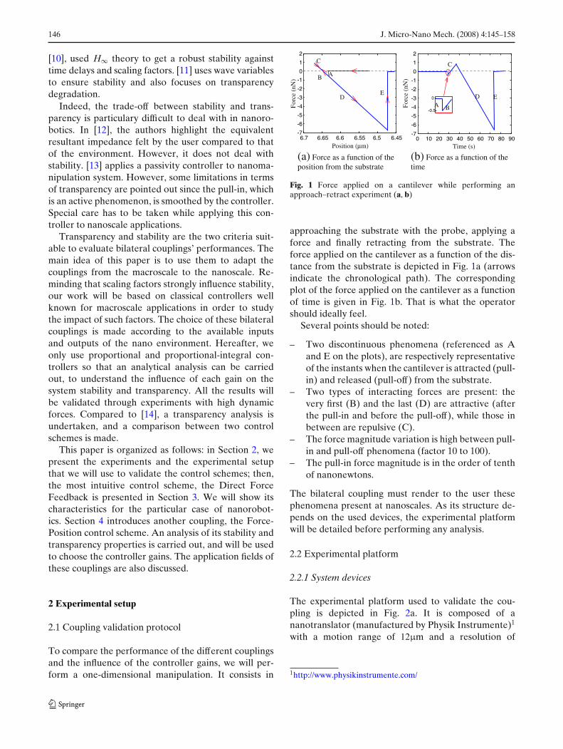
Fig. 1 Force applied on a cantilever while performing anapproach–retract experiment (a, b)
approaching the substrate with the probe, applying aforce and finally retracting from the substrate. Theforce applied on the cantilever as a function of the dis-tance from the substrate is depicted in Fig. 1a (arrowsindicate the chronological path). The correspondingplot of the force applied on the cantilever as a functionof time is given in Fig. 1b. That is what the operatorshould ideally feel.
Several points should be noted:
– Two discontinuous phenomena (referenced as Aand E on the plots), are respectively representativeof the instants when the cantilever is attracted (pull-in) and released (pull-off) from the substrate.
– Two types of interacting forces are present: thevery first (B) and the last (D) are attractive (afterthe pull-in and before the pull-off), while those inbetween are repulsive (C).
– The force magnitude variation is high between pull-in and pull-off phenomena (factor 10 to 100).
– The pull-in force magnitude is in the order of tenthof nanonewtons.
The bilateral coupling must render to the user thesephenomena present at nanoscales. As its structure de-pends on the used devices, the experimental platformwill be detailed before performing any analysis.
2.2 Experimental platform
2.2.1 System devices
The experimental platform used to validate the cou-pling is depicted in Fig. 2a. It is composed of ananotranslator (manufactured by Physik Instrumente)1
with a motion range of 12μm and a resolution of
1http://www.physikinstrumente.com/

J. Micro-Nano Mech. (2008) 4:145–158 147
(a) General view of the plat-form
(b) Haptic interface
Fig. 2 Experimental setup (a, b)
1.83nm. It moves the substrate along the vertical direc-tion, to approach or retract it from a fixed cantilever.
The force applied by the substrate on the cantilever(Fe) is measured with a laser. The deflection of theprobe is measured using a beam focused on the can-tilever, which is reflected onto a photodiode. [15] givesmore details on laser optics. Then the normal force Fe
can be computed from Eq. 1:
Fe = kc d = kc S V (1)
where:
– kc: stiffness of the cantilever (from a hundredthup to several dozen N · m−1) - calibrated as itwas demonstrated in [16]. Note that μN · m−1 ornN · m−1 are also consistent units, more adapted todescribing nanoscale phenomena
– d: deflection of the cantilever– S: sensitivity of the calibrated photodiode– V: measured output voltage
As highlighted in Eq. 1, the force depends on the stiff-ness of the cantilever. This parameter may vary signifi-cantly depending on the performed task. Manipulationoperations require stiff probes to interact precisely withobjects, whereas soft ones can measure smaller forces.Therefore they are suited for exploration or teachingpurposes. The bilateral coupling analysis should takeinto account the cantilever stiffness.
The haptic device used is a 3 degrees of freedomof force feedback Virtuose, manufactured by Haption2
(Fig. 2b).
2.2.2 Power flow
Figure 3 summarizes the power flow between the dif-ferent subsystems (operator, haptic interface, coupling,slave device and environment), and the inputs andoutputs of the subsystems. Fm represents the force fedback to the user, while Vs is the desired velocity set tothe nanotranslator.
The bilateral coupling must be designed accordinglyto the subsystem’s inputs and outputs (master andslave devices’ characteristics, sensors available in theenvironment). However, it is not really restrictive sincemany teleoperation systems for nanoscale applicationspresented in the literature fulfill these requirements[17–19].
2.3 Objectives
The study of the haptic coupling properties will bebased on the classical theory of automation. Our ob-jective is to determine the influence of the differentcontroller gains on the coupling performances. We willuse stability criteria, as Routh-Hurwitz or Llewelyn,and Bode analysis of the transfer functions. The secondstep will be to find the parameters that will lead to
2http://www.haption.com/
Fop Fm
VcVmVm Vs
FeFe
Operator Master device Coupling Slave device Environment
Inputs Outputs
Fe: force applied by the substrate on the cantilever Vc : velocity of the cantilever in the operational space
Fop: force applied by the operator on the master arm Vm : velocity of the master arm in the operational space
Fig. 3 Power flow between the subsystems

148 J. Micro-Nano Mech. (2008) 4:145–158
the most transparent, but still stable, control scheme.This will be done according to the conclusions aboutthe influence of each gain on the system. This proposedtuning must be robust with respect to the environment,and especially the cantilever’s stiffness. Then we willbe able to determine the applications for which thecontrol schemes are the best suited, considering theirintrinsic structure and properties. All these conclusionswill be validated by experiments based on the protocoldescribed in Section 2.1.
3 Direct force feedback
In this section the first control scheme, namely DirectForce Feedback (DFF) is introduced and analysed.Stability (using the Routh-Hurwitz criterion) and trans-parency issues are considered to derive its specificitiesconcerning nanoscale applications. Approach-retractexperiments are conducted using different control pa-rameters to verify the analysis.
3.1 Control scheme structure
This control scheme, depicted in Fig. 4, is the mostintuitive formulation to provide amplified forces tothe operator [20]. Basically, the user operates a hapticdevice in the macro-world to impose the displacementsof the slave device in the nano-world. The blocks andpower flows defined in Fig. 3 are clearly identified. Thecontroller scales down the motions provided by the userby a coefficient Ad, and magnifies environmental forcesby a factor A f to provide force feedback.
The master arm is modeled by a rigid body for whichinertia and damping are respectively Mv and Bv . Theslave robot’s transfer function is modeled by a secondorder function with two time constants τ1 and τ2:
V(s) = [(Bv + Mvs)]−1
N(s) = [(1 + τ1s)(1 + τ2s)]−1 (2)
Vm
V (s)
Fop Fm
1/Ad
Af
VcVs
N (s)
Fe++
Fig. 4 Direct force feedback control scheme
where s is the Laplace variable. Numerical values of theparameters have been identified as:
Mv = 0.4kg ; Bv = 0.1N · s · m−1
τ1 = 1.35 · 10−3s ; τ2 = 0.57 · 10−3s(3)
3.2 Stability
The slave device interacts with a remote environment,which must be considered for the stability analysis.Two approaches can be used. The first is to consider amethod that is applicable for any passive environments(e.g., methods based on passivity analysis). However,they are more conservative since stability is guaranteedfor any environment as long as it is passive. Therefore,they are not useful for our concern to point out thelimitations induced by the cantilever’s stiffness or theenvironment’s characteristics.
The second approach is to model the environmentand to consider stability with respect to the specificitiesof both the coupling and the environment. It will beshown theoretically and experimentally that this con-trol scheme is stable in a given context. To model theenvironment, Assumption 1 is made:
Assumption 1 The slave device is linked with its en-vironment through a spring constant of stiffness kc
(the cantilever). The substrate is modeled as a springks. These two serial springs are linked such that theequivalent stiffness keq is:
1
keq= 1
ks+ 1
kc(4)
Hertz’s theory is widely used to model the contactbetween a cantilever and the substrate [21]. In thecase of a contact between a sphere (which can be theextremity of a cantilever’s tip) and a plane, it states thatthe contact stiffness ks is:
ks = 3
2Ka (5)
The variables are listed below, numerical values aregiven for a silicon cantilever and a glass substrate:
– a: contact area between the sphere and the planea3 = Rt Fe
K– K: equivalent Young’s modulus of the sphere and
the plane K = 134
(1−ν2
1E1
+ 1−ν22
E2
)
– E1,2: Young’s modulus for the cantilever andsubstrate (respectively E1 = 150GPa and E2 =69GPa)

J. Micro-Nano Mech. (2008) 4:145–158 149
– ν1,2: Poisson’s ratio for the cantilever and substrate(respectively ν1 = 0.17 and ν2 = 0.25)
– Rt: sphere’s radius of curvature Rt = 10nm
Even if the Assumption 1 is not very restrictive, itis sufficient to point out the inherent problems of theproposed control scheme in the nano-world. Consider-ing this assumption, and the control scheme depicted inFig. 4, the transfer function between Fop and Vm can bederived. Since the system is linear-time invariant (LTI),the Routh-Hurwitz criterion can be applied to thistransfer function. A necessary and sufficient conditionof stability is:
R = A f
Ad<
γ
keq= Rmax (6)
where γ = Bv(τ1+τ2)[M2v+Mv Bv(τ1+τ2)+B2
vτ1τ2][Mv(τ1+τ2)+Bvτ1τ2]2
As γ only depends on the systems’ parameters, fora given environment, according to Eq. 6 the system’sstability only depends on the ratio A f
Ad.
The worst case for the issue of stability is when theequivalent stiffness is the highest. Using Eq. 4, thiscorresponds to keq = kc. In the following sections wewill use this approximation.
3.3 Transparency
Transparency of haptic couplings is defined in [22, 23].It is based on the comparison between the impedanceof the environment Ze = −Fe/Vc and that felt by theoperator Zop = Fop/Vm. Ideal transparency is achievedwhen:
Zop = Ze (7)
However, for submicron scales, Eq. 7 does not makeany sense. It is necessary to consider the scaling factorsA f and Ad such that the impedances can be compared.In our context, perfect transparency will be achieved if:
Fop
Vm= −A f Fe
AdVc⇔ Zop = A f
AdZe (8)
It has to be noted that the force sensor used modifiesthe profile of the measured forces, and therefore theoperator’s feeling. However, we will not deal with thatissue, as we will focus only on the influence of thecoupling and the haptic device.
Using the control scheme depicted in Fig. 4, theimpedance felt by the operator is derived:
Zop = Fop
Vm= A f
AdZe N(s) + 1
V(s)(9)
3.3.1 Contact
While in contact, the impedance felt by the operatorwill be that of Eq. 9. According to Eq. 8, this corre-
sponds to the impedance he should ideally feel(
A f
AdZe
)modulated by the nanotranslator dynamic. It is alsoinfluenced by the haptic device characteristics.
In the frequency domain (s = jω), Eq. 9 can berewritten as:
Zop = A f
AdZe
1
τ1τ2ω2 + (τ1 + τ2) jω + 1+ (Mv jω + Bv)
(10)
For low frequencies, the impedance Z DF Fop,LF can be
approximated by:
Z DF Fop,LF ≈
ω<<1
A f
AdZe + Bv (11)
The user feels the environmental impedance, as well asthe viscosity of the haptic interface. However, Bv canbe set aside compared to A f
AdZe.
For high frequencies, the impedance Z DF Fop,HF is:
Z DF Fop,HF ≈
ω>>1Mv jω (12)
This result is valid as far as the stiffness of Ze is afinite value. Since Ze can be computed as Ze = keq
jω , andaccording to Assumption 1 keq = kc, Ze ≈
ω>>10.
According to Eq. 12, the transparency of the cou-pling is only affected by the inertia of the haptic devicefor high frequencies.
The Bode’s diagram corresponding to these contactimpedances is plotted in Fig. 5.
-50
0
50
100
150
10-2 10-1 100 101 102 103-270
-180
-90
0
90
Pulsation ω (rad/s)
Phas
e (°
)
Zop
Z DFFop;L F
Z DFFop; H F
A f / Ad . Ze
Mag
nitu
de (
dB)
Fig. 5 Bode’s diagram for contact impedances, DFF controlscheme
150 J. Micro-Nano Mech. (2008) 4:145–158
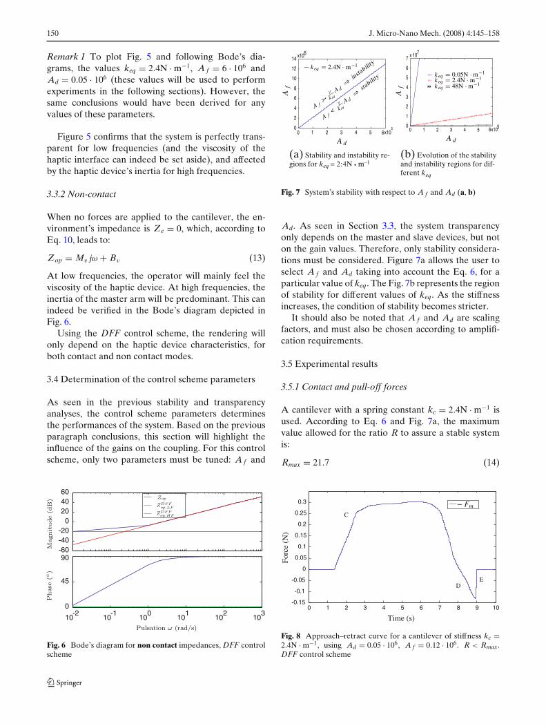
Remark 1 To plot Fig. 5 and following Bode’s dia-grams, the values keq = 2.4N · m−1, A f = 6 · 106 andAd = 0.05 · 106 (these values will be used to performexperiments in the following sections). However, thesame conclusions would have been derived for anyvalues of these parameters.
Figure 5 confirms that the system is perfectly trans-parent for low frequencies (and the viscosity of thehaptic interface can indeed be set aside), and affectedby the haptic device’s inertia for high frequencies.
3.3.2 Non-contact
When no forces are applied to the cantilever, the en-vironment’s impedance is Ze = 0, which, according toEq. 10, leads to:
Zop = Mv jω + Bv (13)
At low frequencies, the operator will mainly feel theviscosity of the haptic device. At high frequencies, theinertia of the master arm will be predominant. This canindeed be verified in the Bode’s diagram depicted inFig. 6.
Using the DFF control scheme, the rendering willonly depend on the haptic device characteristics, forboth contact and non contact modes.
3.4 Determination of the control scheme parameters
As seen in the previous stability and transparencyanalyses, the control scheme parameters determinesthe performances of the system. Based on the previousparagraph conclusions, this section will highlight theinfluence of the gains on the coupling. For this controlscheme, only two parameters must be tuned: A f and
-60-40-20
0204060
10 -2
10 -1
100
101
102
103
0
45
90
Fig. 6 Bode’s diagram for non contact impedances, DFF controlscheme
0 1 2 3 4 5 6x1050
2
4
6
8
10
12
14 x106
Af
A d
k eq 2.4N m 1
A f>
A d
instabilit
y
A f< k eq
k eq
A d
stabilit
y
0 1 2 3 4 5 6x1050
1
2
3
4
5
6
7x 10⁷
xxx
Af
A d
k eq 0.05N m 1
k eq 2.4N m 1
k eq 48N m 1
(a) Stability and instability re-gions for keq = 2:4N • m–1
(b) Evolution of the stabilityand instability regions for dif-ferent keq
Fig. 7 System’s stability with respect to A f and Ad (a, b)
Ad. As seen in Section 3.3, the system transparencyonly depends on the master and slave devices, but noton the gain values. Therefore, only stability considera-tions must be considered. Figure 7a allows the user toselect A f and Ad taking into account the Eq. 6, for aparticular value of keq. The Fig. 7b represents the regionof stability for different values of keq. As the stiffnessincreases, the condition of stability becomes stricter.
It should also be noted that A f and Ad are scalingfactors, and must also be chosen according to amplifi-cation requirements.
3.5 Experimental results
3.5.1 Contact and pull-off forces
A cantilever with a spring constant kc = 2.4N · m−1 isused. According to Eq. 6 and Fig. 7a, the maximumvalue allowed for the ratio R to assure a stable systemis:
Rmax = 21.7 (14)
0 1 2 3 4 5 6 7 8 9 10-0.15
-0.1
-0.05
0
0.05
0.1
0.15
0.2
0.25
0.3
Time (s)
Forc
e (N
)
– Fm
C
DE
Fig. 8 Approach–retract curve for a cantilever of stiffness kc =2.4N · m−1, using Ad = 0.05 · 106, A f = 0.12 · 106. R < Rmax.DFF control scheme

J. Micro-Nano Mech. (2008) 4:145–158 151
Ad is chosen according to the master and slavemotion ranges. To get a good compromise betweeneasiness and accuracy of manipulation, the value Ad =0.05 · 106 is selected (the master motion range corre-sponds then to a displacement of 5μm for the slave).A f is selected so that the system remains stable, i.e. sothat the Routh-Hurwitz criterion given in Eq. 6 is satis-fied. The value A f = 0.12 · 106 will be used.
The obtained results (forces sent back to the user)are depicted in Fig. 8. During the first stage (C), theuser applies forces on the substrate (the maximum is0.30N). While retracting, the user must counterbalancethe forces resulting from the adhesion effects (D). Aforce equal to −0.13N is necessary to release the can-tilever from the substrate (E).
The system remains stable and the forces sent backto the user are equal to those measured by the photodi-ode scaled by A f (Fm = A f Fe according to the controlscheme’s design). Therefore, the operator indeed feelsphenomena happening in the environment. However,using our haptic interface, forces fed back remain toolow to increase the accuracy of the performed task.The force scaling factor has to be increased in order toprovide better force feedback.
During this second experiment, the value of Ad re-mained the same, but A f was increased: A f = 6.0 · 106.With these values:
R = 120 > Rmax (15)
The Routh-Hurwitz criterion is no longer satisfied.Consequently, the system is predicted to be unstable.The results are plotted in Fig. 9.
Remarkably, the forces have been amplified com-pared to the forces in Fig. 8. It is then easier for the
0 1 2 3 4 5 6 7 8 9 10-2
-1
0
1
2
3
4
5
6
7
–
Fig. 9 Approach–retract curve for a cantilever of stiffnesskc = 2.4N · m−1, using Ad = 0.05 · 106, A f = 6 · 106. R > Rmax.DFF control scheme
user to detect repulsive and attractive forces (C, D)and the high variation of the forces due to the pull-off (E). Although force reflection has been improvedby modifying the value of A f , the system’s stability isaffected. When the cantilever establishes contact withthe substrate, it creates high amplitude oscillations inthe system (O). This is very disturbing for the user whohas to act like a damper to absorb the excessive energyresponsible for the instability.
For a given velocity-scaling factor, the DFF controlscheme suffers from a trade-off between stability andforce amplification.
3.5.2 Pull-in, contact and pull-off forces
To render the pull-in force to the user, it is necessaryto increase A f . However, as seen in Eq. 6 and demon-strated in Fig. 9, if Ad is kept constant, the system isunstable. Thus, it should be increased to ensure sta-bility. Since Ad represents the velocity-scaling factor,this implies that the user will need to move the haptichandle over longer distances than in the experimentdepicted in Fig. 8 to perform the same displacement.This makes the experiment very long, as it will bedemonstrated later.
According to Eq. 6, the cantilever stiffness must alsobe considered for stability. Since Fm = A f Fe and Fe =kcd where d is the cantilever deflection, Eq. 6 becomes:
Ad ≥ 1
dFm
γ(16)
For the same value Fm fed back to the user, Ad is pro-portional to the inverse of the deflection. Consideringthe pull-in phenomenon, the deflection of soft can-tilevers is bigger than that of stiff ones. Consequently,
0 10 20 30 40 50 60 70 80 90 100-70
-60
-50
-40
-30
-20
-10
0
10
20
0-2
2
Fig. 10 Approach–retract curve with pull-in for a cantileverof stiffness kc = 0.05N · m−1, Ad = 50 · 106, A f = 6700 · 106.R < Rmax. DFF control scheme

152 J. Micro-Nano Mech. (2008) 4:145–158
the jump into contact will happen when the probeis higher from the substrate. Therefore, the condi-tion on Ad to assure stability is stricter for stiff can-tilevers. We will therefore choose a softer cantilever(kc = 0.05N · m−1).
To be able to feel the pull-in force, we chose A f =6700 · 106 and Ad = 50 · 106. For this cantilever, Rmax =1040. Therefore, for these scaling factors, the system ispredicted to be stable.
The results obtained are presented in Fig. 10. Theforces that should have been sent back to the user, aswell as those actually felt by the operator are shown(i.e., after saturation). As previously explained, thepull-in phenomenon is between 10 to 100 times weakerthan the pull-off. Therefore, if the scaling factors arekept constant, the force corresponding to the pull-off isstrongly amplified and neither the haptic device nor theoperator can cope with such forces. That is why forcesare saturated to 5N, so that the manipulation remainscomfortable for the user. The pull-in effect can clearlybe felt since the peak amplitude is around 2N.
However, since Ad has been increased in order tokeep the system stable, the experiment is time consum-ing (one and a half minutes whereas the cantilever wassoft and initially set very close to the contact point).
The DFF control scheme is highly transparent, sinceboth pull-in and pull-off phenomena were felt. How-ever, it suffers from a trade-off between force ampli-fication and velocity-scaling, which can result either ininstabilities or time consuming experiments. Therefore,for easier manipulations, it is necessary to modify thestructure of the control scheme to add some dampingon the system. This can avoid instabilities that appearin Fig. 9 while reaching the contact.
In Section 4.1, a second well-known control scheme,which takes into account these necessary conditions toavoid the trade-off pointed out above, will be com-pared to the DFF in the special context of micro andnanorobotics.
4 Force-position control
In this section, the Force-Position (FP) control schemeis studied. Stability analysis is conducted using discretetime variable z since it involves numerical integrationswhich make the system very sensitive to the samplingperiod. Transparency analysis is carried out in thecontinuous-time domain in order to compare the resultswith those obtained for the DFF control scheme. Basedon the conclusions, we will choose the gains of the FPcontroller, and we will define what the applications ofsuch a coupling are.
4.1 Control scheme structure
As for the DFF, the inputs of the Force-Position controlscheme are the velocity of the haptic device handle andthe force applied by the environment on the cantilever(Fig. 11). The outputs are the velocity used as thedesired reference for the nanotranslator and the forcethat will be fed back to the user by the haptic device. Aspreviously, A f and Ad are respectively the force andvelocity scaling factors.
Discrete time formulation is used to take into ac-count effects of the sampling period Te. z representsthe discrete time variable. The star superscript is fordiscrete parameters. It was shown in Section 3 that theDFF control scheme presents limitations in terms ofstability, depending on the desired scaling factors. Toimprove this issue, two controllers are added in the FPcoupling. Gn and C(z) are respectively a proportional(P) and a proportional-integral (PI) controller. C(z)
has been discretized using Tustin’s approximation:
C(z) = B fp + K fpTe(z + 1)
2(z − 1)(17)
In the following, V(z) (resp. N(z)) will refer to discretetime transfer functions corresponding to V(s) (resp.N(s)). They are computed using the Z-transform func-tion Z {.}:
V(z) = (1 − z−1)Z{
V(s)s
}= 1
Bv
1 − δ
z − δ(18)
where δ = e− Bv TeMv .
N(z) = 1 − α1z − 1
z − e− Teτ1
− α2z − 1
z − e− Teτ2
(19)
where α1 = 11− τ2
τ1
and α2 = 11− τ1
τ2
.
Compared to the DFF control scheme, the feedbackforce Fm, is computed with the PI controller. Theintegral gain K fp and the proportional gain B fp canbe used to modify the stiffness and damping of therendered force. The gain Gn is used to compute thedesired velocity of the slave device.
1
Fig. 11 Force-position control scheme

J. Micro-Nano Mech. (2008) 4:145–158 153
4.2 Stability
To derive the stability conditions for the FP controlscheme, a first approach is to verify the Routh-Hurwitzcriterion. This method was previously used in Section 3.However, it has been noticed that the environmentmust be modeled. Considering that three gains and twoscaling factors are used in the control scheme depictedin Fig. 11, it is obvious that the relationships betweenthese parameters will be complex and will not allow tohighlight the influence of each of the gains on stability.Therefore, the Routh-Hurwitz criterion is not appropri-ated to analyze the stability of this bilateral coupling.
To assure the system’s stability without modeling theenvironment, two main approaches are currently used.The first is passivity [7], which deals with energy flow inthe system. The second is absolute stability [24]. As forpassivity, it ensures that if the control scheme is con-nected to passive blocks (in our case the environmentand the operator which can be considered passive asin [25]), the system will remain stable. Both of thesecriteria lead to sufficient but not necessary conditions.Since absolute stability is less conservative, we will usethis criterion, based on Llewelyn’s theorem.
The admittance matrix �P of the coupling is definedas:[
V∗m
V∗c
]= �P(z) ·
[F∗
op
F∗e
]
=[
p11(z) p12(z)
p21(z) p22(z)
]·[
F∗op
F∗e
] (20)
where:
p11(z) = V(z) [A f + Ad Gn C(z)]/D(z)
p12(z) = [A f Ad Gn C(z) V(z)]/D(z)
p21(z) = [Gn V(z) C(z)]/D(z)
p22(z) = A f Gn[1 + C(z) V(z)]/D(z)
D(z) = A f + Ad Gn C(z) + A f V(z) C(z)
Theorem 1 (Llewelyn [26])A system represented by the admittance matrix �P
is unconditionally stable if and only if the followingconditions hold:
C1 = Re(p11) ≥ 0 (21)
C2 = Re(p22) ≥ 0 (22)
C3 = 2Re(p11)Re(p22) − |p12 p21| − Re(p12 p21) ≥ 0
(23)
These inequalities will be used to verify if the chosengains meet stability requirements.
4.3 Transparency
In order to compare the results to those obtained forthe DFF, transparency was studied in the continuoustime domain. Using the control scheme depicted inFig. 11, the impedance felt by the operator Zop =Fop/Vm can be computed:
Zop = nze Ze + A f C(s)V(s) + A f + AdGnC(s)dze Ze + A f V(s) + AdGnC(s)V(s)
(24)
where:
nze = A f GnC(s)V(s)N(s) + A f Gn N(s) (25)
dze = A f GnV(s)N(s) (26)
4.3.1 Contact
When the contact is established, Z F Pop,LF can be com-
puted for low frequencies:
Z F Pop,LF ≈
ω<<1
A f
Ad + A f keq
K fp
Ze (27)
As K fp increases, the impedance felt by the operatortends to the ideal impedance A f
AdZe.
For high frequencies, the impedance Z F Pop,HF felt by
the user is:
Z F Pop,HF ≈
ω>>1Mv jω (28)
For the same reasons as the ones exposed in Section3.3.1, the user only feels the inertia of the haptic devicefor ω >> 1.
Bode’s diagram represented in Fig. 12 is useful toillustrate the analytical results, and to compare them tothose obtained for the DFF control scheme.
Fig. 12 Bode’s diagram for contact impedances, FP controlscheme

154 J. Micro-Nano Mech. (2008) 4:145–158
Remark 2 Bode’s diagram (Fig. 12), and followingshave been plotted for specific values: keq = 2.4N · m−1,A f = 6 · 106, Ad = 0.05 · 106 (the same values as forFig. 5), K fp = 100N · m−1, B fp = 2N · s · m−1 and Gn =48.0m · N−1 · s−1. As already underscored in remark 1,these values are only defined to illustrate the commen-tary, but do not change the conclusions.
For low frequencies, the variations in the Bode’smagnitude are the same for the simulated contact im-pedance and for the environment. The real and feltimpedances only differ by a static gain which can bereduced by increasing K fp. Consequently, when theuser reaches the contact point, he is able to detect thevariations of the forces involved during the process.Although the system is not as perfectly transparent asDFF, it is well suited for manipulation tasks.
4.3.2 Non-contact
When no force is acting on the cantilever, the operatorfeels the impedance:
Zop = A f(K fp + B fp jω
)A f jω + AdGn
(K fp + B fp jω
) + Mv jω + Bv
(29)
For low frequencies, the impedance Z F Pop,LF can be
approximated from:
Z F Pop,LF ≈
ω<<1
A f
AdGn+ Bv (30)
To minimize the impedance felt by the operator, with-out affecting the scaling factors, Gn is the only para-meter that can be tuned. The higher it is, the betterthe transparency will be. However, whatever the valuesof the control scheme’s gains, the user will feel theviscosity of the haptic interface (as was the case for theDFF control scheme).
At higher frequencies, he feels the impedanceZ F P
op,HF :
Z F Pop,HF ≈
ω>>1Mv jω (31)
As for the DFF, the operator will feel the inertia of thehaptic device.
The Bode’s diagram (Fig. 13) confirms the validityof the approximations made in Eqs. 30 and 31. Whencompared to the Bode’s diagram for the DFF controlscheme (Fig. 6) for non-contact, it highlights the lack oftransparency for low frequencies. However, this differ-ence can be reduced by increasing Gn.
Fig. 13 Bode’s diagram for non contact impedances, FP controlscheme
As highlighted in Table 1 which summarizes theapproximated impedance for the DFF and FP controlschemes, the FP coupling is less transparent than theDFF. To obtain the same transparency K fp has to behigh enough to ensure a stiff contact, while Gn willinfluence the non-contact behavior of the coupling. Thehigher it is, the less viscous the feeling for the operatorwill be.
4.4 Determination of the control scheme parameters
The performance of this bilateral coupling highly de-pends on the controller parameters and the scalingfactors (see Sections 4.2 and 4.3). However, relationsderived in the previous sections do not allow to easilychoose the gains since each of them is composed ofmany parameters. It will be useful to consider particularcases to derive simple necessary conditions of stability.Using these relations, and transparency considerations,gains will be chosen. Then, Llewelyn criterion willbe used to see if the gains meet sufficient stabilityconditions.
Table 1 Approximated values of Fop for DFF and FP controlschemes
DFF FP
Non- Low BvA f
AdGn+ Bv
contact frequenciesHigh Mv jω Mv jω
frequencies
Contact LowA fAd
Ze + BvA f K fp
Ad K fp+A f keqZe
frequenciesHigh Mv jω Mv jω
frequencies

J. Micro-Nano Mech. (2008) 4:145–158 155
4.4.1 Scaling factors
As in the first control scheme, A f and Ad depend onuser’s requirements. Indeed, one might want a precisepositioning, and/or important force feedback, accord-ing to the manipulation tasks. As in Section 3, wewill choose Ad = 0.05 · 106. A f will be such that theforces sent back to the user are high enough for anuntrained user to distinguish the different phenomenaencountered during the experiment.
4.4.2 Proportional controller Gn
Problems of stability can be due to control schemes butalso to numerical computation. Indeed, the force F∗
m attime k + 1 is determined using information of positionsand velocities at time k (see Fig. 11):
F∗m(k + 1) = B fpΔV(k) + K fpΔX(k) (32)
where:
ΔV(k) = AdV∗s (k) − V∗
m(k)
ΔX(k) = Ad X∗s (k) − X∗
m(k)(33)
For similar reasons, the expression of V∗s is:
V∗s (k + 1) = Gn
[F∗
e (k) − 1
A fF∗
m(k)
](34)
Considering Eqs. 32 and 34 and the fact that the posi-tion X∗
s is computed using Tustin’s discretization, whenthe probe is well above the substrate (no force appliedon it, i.e. F∗
e = 0), F∗m is given by:
F∗m(k + 1) = λ1 F∗
m(k − 1) + λ2V∗m(k) + (λ3 + λ4) K fp
(35)
where:
λ1 = −Gn
[B fp Ad + K fp Ad
Te2
A f
]
λ2 = −[
B fp + K fpTe
2
]
λ3 = Ad
[X∗
s (k − 1) + V∗s (k − 1)Te
2
]
λ4 = −[
X∗m(k − 1) + V∗
m(k − 1)Te
2
]
Avoiding numerical instabilities leads to an upperbound on Gn, a necessary condition for stability:
|λ1| < 1 ⇔ Gn <A f
Ad K fpTe2 + Ad B fp
= Gnlim (36)
4.4.3 Proportional integral controller B fp and K fp
In [27] a relation between B fp, K fp and Te is derivedto assure the stability of the system while in contactwith a rigid environment. In that work, the authorsapply the Routh-Hurwitz criterion to a control schemesimilar to ours. However, the output of the couplingis the position Xm instead of the velocity Vm and thebackward difference is used to determine the discretecontroller C(z) (instead of Tustin).
We will use the same methodology applied to oursystem. As for the DFF control scheme, the systemconsidered is LTI. The discrete time transfer functionis:
V∗m
F∗op
= V(z)
1 + V(z)C(z)(37)
Before applying the Routh-Hurwitz criterion onthe characteristic equation, a bilinear transformation(
z = 2+wTe2−wTe
)should be made. It leads to:
b 2w2 + b 1w + b 0 = 0 (38)
where:
b 2 = 4Bv(1 + δ) − 4(1 − δ)B fp (39)
b 1 = (1 − δ)(4Bv + 4B fp − 2K fpTe) (40)
b 0 = 2K fpTe(1 − δ) (41)
The Routh-Hurwitz criterion is achieved if and only ifb 0, b 1 and b 2 have the same sign. Since δ < 1, Eq. 41 isalways positive. Therefore, the system will be stable ifand only if b 1 > 0 and b 2 > 0, which implies:
Bv + B fp >K fpTe
2(42)
Bv
1 + δ
1 − δ> B fp (43)
Equation 42 is the same condition as that found in [27]and states that the stiffness of the coupling is boundedby the inherent damping of the haptic interface and thatadded by the coupling. Moreover, if the sampling pe-riod increases, K fp must decrease for the same amountof damping to guarantee stability.
Using the first order Taylor development of x �→exp(x) in the region of 0
(Bv TeMv
→ 0 since Te → 0)
,
δ ≈ 1 − Bv TeMv
. Equation 43 can be approximated by:
2Mv
Te> Bv + B fp (44)
This highlights that the maximum damping (and there-fore, according to Eq. 42, the maximum stiffness) ad-missible is limited by the inertia of the master arm

156 J. Micro-Nano Mech. (2008) 4:145–158
and is inversely proportional to the sampling period Te.This is a convincing argument of the importance of thesampling period for stable haptic feedback.
4.4.4 Summary
The relations derived in Section 4.3 as well as inSections 4.4.2 and 4.4.3 are summarized in the Table 2.The minimum and maximum values each gain can taketo ensure necessary stability conditions are given, aswell as transparency considerations.
As seen in Section 4.4.2, Gn has to be high to al-low a transparent non contact behavior. According toEq. 36, for stability reasons, Gn must be smaller than
A f
Ad K fpTe2 +Ad B fp
. Therefore, smaller values for B fp and
K fp allow for a higher Gnlim , and increase the noncontact transparency.
Concerning K fp, a maximum value to verify theRouth-Hurwitz criterion is derived. However, as ex-plained above, for transparency reasons K fp shouldbe low enough to limit the viscosity when there is nocontact.
4.5 Experimental results
To compare the results with the ones obtained withthe DFF control scheme we use the same cantileveras in Section 3.5.1 (kc = 2.4N · m−1), with the samescaling factors (Ad = 0.05 · 106, A f = 6 · 106). Otherparameters are chosen according to the results of thetransparency and stability analysis (Table 2).
A good compromise for transparency in contact andnon contact mode is found if K fp = 100N · m−1. Thisvalue is indeed smaller than the maximum allowedvalue 4Mv
T2e
. Enough damping is introduced by choosing
B fp = 2.0N · s · m−1. It is greater than the minimumvalue K fpTe
2 − Bv = 0.15N · s · m−1 and non contacttransparency is still good. Gn is chosen such that Gn =0.90Gnlim = 48.0m · N−1 · s−1.
Table 2 Valid range of values for FP controller gains
Minimum value Maximum value
K fp High for a stiff Eq. 42, 44 → 4Mv
T2e
contact feeling(Section 4.3.1)
B fp Eq. 42→ K fpTe2 − Bv Low for non contact
transparency(Section 4.3.2)
Gn High for non contact Eq. 36 → A f
Ad K fpTe2 +Ad B fptransparency
(Section 4.3.2)
Fig. 14 Values of C1, C2 and C3 with respect to ω
The selected parameters must satisfy Eqs. 21, 22 and23 to ensure that the system will remain stable whateverthe environment. In order to check such conditions, thevalues of C1, C2 and C3 are plotted in the frequencydomain. The results are given in Fig. 14.
For pulsations lower than ωc = 35rad · s−1, C1, C2,and C3 are positive: Llewelyn’s criterion is verified.According to the system bandwidth, pulsations greaterthan ωc will be attenuated, therefore the system willremain stable with the chosen values.
To verify experimentally that the gains we choseare adapted to the stated problem, we performed thesame approach-retract operation as in Section 3. Theresults obtained are plotted in Fig. 15. The forces feltby the operator, as well as those measured by the force
20 4 6 8 10-2
-1
0
1
2
3
4
5
Time (s)
For
ces
(N)
–Fm
A f Fe
Fig. 15 Approach–retract curve for a cantilever of stiffnesskc = 2.4N · m−1, using Ad = 0.05 · 106, A f = 6 · 106. FP controlscheme

J. Micro-Nano Mech. (2008) 4:145–158 157
sensor (and scaled by A f ) are represented. They mustbe compared to those in Fig. 9. The system remainedstable during this experiment, contrary to the DFFcontrol scheme. Moreover, even if the force sent backto the user is computed through the control scheme(and not directly fed back), the feeling that the operatorgot reflects what happened in the remote environmentsince Fm and A f Fe plots are similar. The oscillationsthat can be seen in Fm’s plot were induced by the virtualcoupling. Since the bandwidth of the haptic device islimited, they were not disturbing for the user. There-fore, although this control scheme is less transparentthan the DFF, the feeling is good enough to allow theoperator to feel the pull-off phenomenon with a peak ofamplitude 1N. Consequently, the analysis performed inthis paper allows for an efficient tuning of the controllerpresented in Section 4.1.
The pull-in phenomena is not visible on Fig. 15.Indeed, to avoid time-consuming manipulations, wechose Ad = 0.05 · 106 (i.e., such that a velocity of1cm · s−1 of the haptic handle represents 0.2μm · s−1 forthe slave device). With this value of Ad, the velocityof the nanotranslator was too high compared to thedynamics of the pull-in effect and thus could not bereflected to the user.
To prove the robustness of our approach with re-spect to the environment’s stiffness, the same exper-iment was performed using different cantilevers. Theresults are presented in Fig. 16. The same velocity-
0 05 1
2 4 1
48 1
Fig. 16 Approach–retract curve for cantilevers of stiffnesseskc = 0.05N · m−1 (K fp = 100N · m−1, B fp = 1.2N · s/m, Gn =2329m/N · s), kc = 2.4N · m−1 (K fp = 100N · m−1, B fp = 2.0N ·s · m−1, Gn = 48.0m · N−1 · s−1), and kc = 48N · m−1 (K fp =100N · m−1, B fp = 1.5N · s · m−1, Gn = 1.98m · N−1 · s−1). FPcontrol scheme
scaling factor was used for the three probes. The forceamplification was chosen so that the user could clearlyfeel the contact (about 5N were fed back via the hapticdevice), for a cantilever’s deflection smaller than 5μm.This lead to A f = 200 · 106 for the cantilever of stiff-ness kc = 0.05N · m−1, and A f = 0.2 · 106 for stiffnesskc = 48N · m−1. Other gains were chosen using Table 2.
It should be noted that these experiments were per-formed in a non-controlled environment. Conditionsof humidity and temperature may have changed be-tween the experiments. However, the pull-off was in-deed greater for cantilevers with a low stiffness. Asnoted above, the oscillations on the plots of Fig. 16 areinduced by the virtual coupling, but are not disturbingfor the operator due to the limited bandwidth of thehaptic device.
The FP control scheme is adapted to nanomanip-ulations, especially because the system is stable, evenwhen in contact with the substrate, for cantilevers withstiffnesses of 0.05N · m−1 up to 48N · m−1. Moreover,the analysis is validated experimentally. Forces of 10nN(pull-off for the cantilever of stiffness kc = 0.05N · m−1)were felt by the user.
5 Conclusion
Two different control schemes have been analysed inthis paper, in the particular context of nanorobotic ap-plications. The Direct Force Feedback control schemesuffers from a trade-off between stability and forceamplification if time consuming manipulations have tobe avoided. However, transparency is high as provenanalytically, and underscored by the fact that we wereable to feel both pull-in (forces of 0.5nN) and pull-off phenomena. Using Force-Position control scheme,higher force amplification without suffering from theduration of the manipulation can be achieved. Forcesof 10nN were felt by the user and stable contact forcantilevers of stiffnesses from 0.05N · m−1 to 48N · m−1
was demonstrated.The choice of the control scheme will therefore de-
pend on the relevant application. For a highly trans-parent rendering, DFF is appropriate, however theexperiments will be time-consuming. For a more com-plex task, implying high displacements, the FP controlscheme should be chosen. It will greatly improve theoperator’s ability by providing him or her with forcefeedback.
Using the analysis carried out, the influence of eachgain on the bilateral coupling is highlighted. These re-sults will therefore help to realize real-time adaptationof the gains.

158 J. Micro-Nano Mech. (2008) 4:145–158
Notations
Fop/Fe/Fm User/environment/master forceXs/Xm Slave/master positionVs/Vc/Vm Slave/cantilever/master velocityZop/Ze User/environment impedanceZ DF F
op,LF/Z DF Fop,HF Low/high frequencies user’s imped-
ance for DFFZ F P
op,LF/Z F Pop,HF Low/high frequencies user’s imped-
ance for FPks/kc/keq Contact/cantilever/equivalent
stiffnessd Cantilever’s deflectionMv/Bv Master’s inertia/viscosityτi i-th time constant of the
nanotranslatorV(s)/N(s) Virtuose/nanotranslator transfer
functionTe Sampling periodA f /Ad Force/velocity scaling factorC(s)/C(z) Continuous/discrete PI controllerB fp/K fp Proportional/integral gainGn Proportional controller
Acknowledgements This work was supported by the FrenchNational Agency of Research, through the PACMAN project.
References
1. Sitti M (2007) Microscale and nanoscale robotics systems[grand challenges of robotics]. IEEE Robot Autom Mag14(1):53–60
2. Ferreira A, Mavroidis C (2006) Virtual reality and haptics fornanorobotics. IEEE Robot Autom Mag 13(3):78–92
3. Hollis R, Salcudean S, Abraham D (1990) Toward a tele-nanorobotic manipulation system with atomic scale forcefeedback and motion resolution. In: IEEE workshop on mi-cro electro mechanical systems, Napa Valley, 12–14 February1990, pp 115–119
4. Goldfarb, M (1998) Dimensional analysis and selective dis-torsion in scaled bilateral telemanipulation. In: Proceedingsof the IEEE international conference on robotics and au-tomation. IEEE, Piscataway, pp 1609–1614
5. Niemeyer G, Slotine JJ (1991) Stable adaptive teleoperation.IEEE J Oceanic Eng 16(1):152–162
6. Anderson R, Spong M (1989) Bilateral control of teleoper-ators with time delay. IEEE Trans Automat Contr 34(5):494–501
7. Ryu JH, Kim YS, Hannaford B (2004) Sampled- andcontinuous-time passivity and stability of virtual environ-ment. IEEE Trans Robot Autom 20(4):772–776
8. Daunay B, Micaelli A, Régnier S (2007) 6 DOF haptic feed-back for molecular docking using wave variables. In: Pro-ceedings of the IEEE international conference on roboticsand automation. IEEE, Piscataway, pp 840–845
9. Kim SG, Sitti M (2006) Task-based and stable telenanoma-nipulation in a nanoscale virtual environment. IEEE TransAutom Sci Eng 3(3):240–247
10. Boukhnifer M, Ferreira A (2007) H-infinity loop shaping bi-lateral controller for a two-fingered tele-micromanipulationsystem. IEEE Trans Control Syst Technol 15(5):891–905
11. Boukhnifer M, Ferreira A (2006) Wave-based passivecontrol for transparent micro-teleoperation system. RobotAuton Syst 54(7):601–615
12. Kaneko K, Tokashiki H, Tanie K, Komoriya K (1997) Im-pedance shaping based on force feedback bilateral controlin macro-micro teleoperation system. In: Proceedings of theIEEE international conference on robotics and automation.IEEE, Piscataway, pp 710–717
13. Onal CD, Sitti M (2009) A scaled bilateral control systemfor experimental one-dimensional teleoperated nanomanip-ulation. Int J Rob Res 28(4):484–497
14. Venture G, Haliyo DS, Régnier S, Micaelli A (2005)Force-feedback micromanipulation with unconditionally sta-ble coupling. In: Proceedings of the IEEE/RSJ interna-tional conference on intelligent robots and systems. IEEE,Piscataway, pp 1923–1928
15. Tian X, Liu L, Jiao N, Wang Y, Dong Z, Xi N (2004) 3Dnano forces sensing for an AFM based nanomanipulator.In: Proceedings of the IEEE international conference on in-formation acquisition. IEEE, Piscataway, pp 208–212
16. Xie H, Vitard J, Haliyo DS, Régnier S, Boukallel M (2008)Calibration of lateral force measurements in atomic forcemicroscopy. Rev Sci Instrum 79:033708
17. Onal CD, Pawashe C, Sitti M (2007) A scaled bilateralcontrol system for experimental 1-D teleoperated nanoma-nipulation applications. In: Proceedings of the IEEE/RSJinternational conference on intelligent robots and systems.IEEE, Piscataway, pp 483–488
18. Ammi M, Ferreira A (2007) Robotic assisted micromanipula-tion system using virtual fixtures and metaphors. In: Proceed-ings of the IEEE international conference on robotics andautomation. IEEE, Piscataway, pp 454–460
19. Ando N, Ohta M, Hashimoto H (2000) Micro teleopera-tion with haptic interface. In: 26th annual conference of theIEEE industrial electronics society, vol 1. IEEE, Piscataway,pp 13–18
20. Goethals P, Gersem GD, Sette M, Reynaerts D, BrusselHV (2007) Accurate haptic teleoperation on soft tissuesthrough slave friction compensation by impedance reflec-tion. In: Proceedings of the second joint EuroHapticsconference and symposium on haptic interfaces for vir-tual environment and teleoperator systems, Tsukuba, 22–24March 2007
21. Maugis D (2000) Contact, adhesion and rupture of elasticsolids, vol 130, chap 4. Springer, New York pp 203–344
22. Lawrence D (1993) Stability and transparency in bilat-eral teleoperation. IEEE Trans Robot Autom Autom 9(5):624–637
23. Hokayem PF, Spong MW (2006) Bilateral teleoperation: anhistorical survey. Automatica 42(12):2035–2057
24. Adams RJ, Hannaford B (1999) Stable haptic interactionwith virtual environments. IEEE Trans Robot Autom Autom15(3):465–474
25. Hogan N (1989) Controlling impedance at the man/machineinterface. In: Proceedings of the IEEE international con-ference on robotics and automation. IEEE, Piscataway,pp 1626–1631
26. Llewellyn F (1952) Some fundamental properties of transmis-sion systems. Proc IRE 40(3):271–283
27. Gil JJ, Avello A, Rubio A, Flórez J (2004) Stabilityanalysis of a 1 DOF haptic interface using the Routh-Hurwitz criterion. IEEE Trans Control Syst Technol 12(4):583–588