Analysis of Spatially Varying Relationships BetweenUrban Environment Factors And Land SurfaceTemperature In Mashhad City, IranHadi Soltanifard 

Hakim Sabzevari UniversityAbdolreza Kashki 

Hakim Sabzevari UniversityMokhtar Karami  ( M.Karami08@yahoo.co.uk )

Hakim Sabzevari University https://orcid.org/0000-0001-8336-3621

Research Article

Keywords: Land Surface Temperature (LST), Geographically Weighted Regression (GWR), Ordinary LeastSquare (OLS), Neighborhood Scale, Mashhad

Posted Date: November 3rd, 2021

DOI: https://doi.org/10.21203/rs.3.rs-927611/v1

License: This work is licensed under a Creative Commons Attribution 4.0 International License.  Read Full License

1

Analysis of spatially varying relationships between urban environment factors

and land surface temperature in Mashhad city, Iran

Hadi Soltanifarda, Abdolreza Kashki b, Mokhtar Karami*b

a- Department of Environment, Hakim Sabzevari University, Sabzevar, Khorasan Razavi, Iran

b - Department of Climatology, Hakim Sabzevari University, Sabzevar, Khorasan Razavi, Iran

b*- The corresponding author: Department of Climatology, Faculty of Geography & Environmental Sciences,

Hakim Sabzevari University, Sabzevar, Iran

Tel: 0098 51 44013223, 0098 9156537277 Fax: 0098 51 44013223

M.Karami@hsu.ac.ir, M.Karami08@Yahoo.co.uk

Abstract

Land Surface Temperature (LST), in particular for the urban environment, is a key indicator to characterize

urban heat changes, urban climate, global environmental change, and human-environment interactions.

However, due to differences in the local spatial variations of LST and the related influence factors, few

studies have discussed the spatial non-stationarity and spatial scale effects within urban areas. Moreover,

in cities such as Mashhad, which are located in a hot and dry climate, have been less studied of the

relationship between LST and urban influencing factors on a neighborhood scale. In the present study, the

spatial distribution of the mean LST was evaluated in association with the 16 explanatory indices at the

neighborhood's level in Mashhad City, Iran, as a case study. To assess the main components contributing

to the LST variations, Principal Components Analysis (PCA) was employed in this study. Additionally,

Ordinary Least Square (OLS) and Geographically Weighted Regression (GWR) models were used to

explore the spatially varying relationships and identify the model's efficiency at the neighborhood's scale.

Our findings showed the five most important components contributing to LST variances, explaining 86.2%

of the variability. The most negative relationship was observed between LST and the morphological

features of neighborhoods (PC3). In contrast, the landscape composition of the green patches (PC2)

exhibited the lowest negative impacts on LST changes. Moreover, road and traffic density characteristics

of the neighborhoods (PC4) were the only effective components to alert the average LST positively. With

R2= 0.678, AIC c= 2125.6, and Moran's I= 0.018, the results revealed that the GWR model had better

efficiency than the corresponding non-spatial OLS model in terms of the goodness of fits. It suggests that

the GWR model has more ability than the OLS one to predict LST intensities and characterize spatial non-

stationary. Therefore, it can be applied to adapt more effective strategies in planning and designing the

urban neighborhoods for mitigation of the adverse heat effects.

Keywords: Land Surface Temperature (LST), Geographically Weighted Regression (GWR), Ordinary

Least Square (OLS), Neighborhood Scale, Mashhad

2

1. Introduction

For a long period, an increasing number of studies have been conducted to reveal the relationship

between LST and driving factors in various disciplines. However, concerning urban studies, LST

has been considered as a fundamental parameter for controlling the physical, chemical, and

biological processes of the Earth's surface (Pu, Gong, Michishita, & Sasagawa, 2006). According

to the type of relations, trends, and corresponding effects, these studies can be divided into three

main distinct categories. The first group includes the causality studies mainly focused on the

associations between LST and urban environment components. These works particularly have a

wide range of urban morphology indices, vegetation index, landscape metrics, spatial patterns of

Urban Green Spaces (UGS), and climatic characteristics (Y. Wang, Chau, Ng, & Leung, 2016).

The second group involves the investigations reported the temporal variability of LST based on

remotely sensed observation methods and time series analysis (Eleftheriou et al., 2018; Weng, Fu,

& Gao, 2014; Y. Zhang, Odeh, & Han, 2009; G. Zhao et al., 2017). Finally, the third group of

studies deals with the environmental, social, and economic impacts of LST on cities developed in

various interdisciplinary fields. Specifically, common results the negative effects on social

interactions, public health, and heat mortality consequently(C. Huang et al., 2011; G. Huang, Zhou,

& Cadenasso, 2010; Madrigano, Ito, Johnson, Kinney, & Matte, 2015; White-Newsome et al.,

2013). Moreover, extensive researches have been devoted to the role of LST in rising the citizen's

economic expenses, in particular by energy consumption, more demands for energy, and the

related costs (Carnielo & Zinzi, 2013; Hirano & Fujita, 2012; Santamouris, Cartalis, Synnefa, &

Kolokotsa, 2015). Additionally, many existing studies have been performed to find out the adverse

effects of LST on the urban environment, including air pollution, climate changes, and human

comfort (Akbari, 2007; Fallmann, Forkel, & Emeis, 2016; Ferreira, Helena, & Duarte, 2019; H. Li

et al., 2018; Shaharuddin, Noorazuan, Takeuchi, & Noraziah, 2014; Z. Song et al., 2018).

Although most of the mentioned studies refer to the various number of variables, the findings

mainly include the analysis of the bivariate relationship without considering the confounding effect

of other variables. Indeed, using spatial data, acquired directly from the remotely sensed cases, has

been established to be non-stationary and varied in geographic characteristics (Su, Foody, &

Cheng, 2012). Besides, the results of conventional statistical methods such as the Ordinary Least

Squares (OLS) may not reflect all the key details of the relationships between variables if the non-

3

stationary spatial property of data is not considered as a major limitation when geo-referenced data

are applied (Brown et al., 2012; Brunsdon, Fotheringham, & Charlton, 1996; Luo & Peng, 2016).

Recently, a non-parametric technique has been developed by Brundson, Charlton, and

Fotheringham to overcome this problem by extending traditional standard global regression

approaches. OLS compared to Geographically Weighted Regression (GWR), considers the spatial

structure of data in the modeling. GWR as a local approach is an effective model able to represent

the spatial variations to explore the potential relationship between variables (Y. Huang, Yuan, &

Lu, 2019; Z. Wang, Fan, Zhao, & Myint, 2020). GWR provides extra information on the spatial

processes by a local model of the variables, varying over space to detect locally different

parameters with spatial dependence and heterogeneity of regions (Fotheringham, Brunsdon, &

Charlton, 2003; Harris, Fotheringham, Crespo, & Charlton, 2010). Particularly, this approach

enables measuring the spatial instability of coefficient over the study area regarding LST and the

urban environment variables, tending to be spatially varied by the type and local conditions like

activities, ecological and morphological patterns.

The present study is carried out at the neighborhood scale to evaluate the effects of different

indicators of the urban environment on LST in Mashhad city, Iran. This study aims to achieve the

following objectives: 1) investigating the spatial non-stationarity modeling by GWR in the

relationships between LST and the urban environment indicators; 2) choosing a good fitting model

for comparing GWR and OLS; 3) examining the spatial distributions of LST and the impact

factors; 4) exploring the relationships at the neighborhood scale to adopt proper strategies for heat

mitigation and urban warming.

In this study, the characteristics of the urban environment, in particular, were identified by 16

indicators, implying various aspects of natural and physical elements, including built-up areas,

streets, spatial configuration, land use, and landscape. Furthermore, the GWR model was used to

highlight the details of spatial information and enhance the accuracy of relationships between the

variables. Due to variation and complexity in the selected urban datasets, redundancy and

multicollinearity problems may be added to the difficulty in interpreting the relationships between

the influencing variables. Therefore, Principal Component Analysis (PCA) was used in

combination to reduce the data dimensionality and complexity. This pre-analysis helped to

organize a large number of variables into a few and more informative groups. Moreover, the

4

current work applied the ordinary least square (OLS) to compare to the findings of the GWR

concerning residual spatial autocorrelation, allowing to find a goodness-of-fit model. This has been

explained in detail in the research method section.

Briefly, many scholars have applied the GWR model to explore the relationship between LST and

urban factors or explanatory variables in recent years (Kalota, 2017; S. Li, Zhao, Miaomiao, &

Wang, 2010; Luo & Peng, 2016; Su et al., 2012; Z. Wang et al., 2020; C. Zhao, Jensen, Weng, &

Weaver, 2018). Although, in the recent literature, the related advantages of the GWR model have

been well-documented over those of the other models, utilizing the idea of the GWR in

combination with PCA concerning LST and the urban variables has rarely been discussed. Also, a

lack of the scale's investigations concerning urban study is observed; however, this study is

prominently at the neighborhood scale for better understand the distributions of LST, urban

indicators, and existing relationships, as the neighborhood scale reveals more details. Therefore,

the neighborhood scale can improve our knowledge concerning the driving mechanisms behind

the formation of thermal environments and relative changes. Besides, the related findings can fill

the gap in the corresponding scale and significantly formulate urban planning policies to alleviate

LST effects. This study presents findings that are of major significance to climate experts, urban

and regional planners, environmentalists, and policymakers to explore measures for mitigating

uncontrolled urban expansion and thermal discomfort in Mashhad City.

2. Methods

2.1.study area

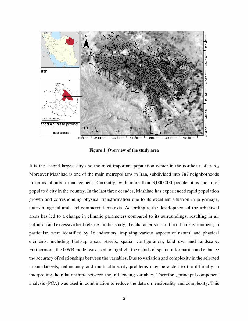
Mashhad, covering an area of 215 sq. km, is located at the northeast of Iran between 59°03′ to

60°35' E longitudes and 35°42′ and 36°59' N latitudes in the Khorasan Razavi province (Figure 1).

With a height of 970 meters, the city has a cool-dry climate with warm-dry summers and cold-

humid winters. The average temperature is 15℃, with 233.8 mm annual rainfall and 53% relative

humidity. Moreover, the number of freezing days per year for this city amounts to 85 days.

5

Figure 1. Overview of the study area

It is the second-largest city and the most important population center in the northeast of Iran و

Moreover Mashhad is one of the main metropolitans in Iran, subdivided into 787 neighborhoods

in terms of urban management. Currently, with more than 3,000,000 people, it is the most

populated city in the country. In the last three decades, Mashhad has experienced rapid population

growth and corresponding physical transformation due to its excellent situation in pilgrimage,

tourism, agricultural, and commercial contexts. Accordingly, the development of the urbanized

areas has led to a change in climatic parameters compared to its surroundings, resulting in air

pollution and excessive heat release. In this study, the characteristics of the urban environment, in

particular, were identified by 16 indicators, implying various aspects of natural and physical

elements, including built-up areas, streets, spatial configuration, land use, and landscape.

Furthermore, the GWR model was used to highlight the details of spatial information and enhance

the accuracy of relationships between the variables. Due to variation and complexity in the selected

urban datasets, redundancy and multicollinearity problems may be added to the difficulty in

interpreting the relationships between the influencing variables. Therefore, principal component

analysis (PCA) was used in combination to reduce the data dimensionality and complexity. This

6

pre-analysis helped to organize a large number of variables into a few and more informative

groups. Moreover, the current work applied the ordinary least square (OLS) to compare to the

findings of the GWR concerning residual spatial autocorrelation, allowing to find a goodness-of-

fit model.

2.2.Derivation and selection of variables

In the present work, two different types of datasets, namely primary and secondary data, were

utilized. Primary datasets included Landsat image, Landsat Operational Land Imager (OLI),

Thermal Infra Red Sensor (TIRS), land use map, population, road network, and traffic. To obtain

better results in this study, LST was processed later using the maximum likelihood classification

in ENVI software.

2.2.1. Dependent variable: LST

Landsat 8 image was launched on 14 September 2019 from the Earth Explorer website to estimate

the LST. With the spatial resolution of 100m, the thermal infrared sensor (TIRS) band (band 10)

was employed to enable the atmospheric correction of the thermal data and retrieve LST with

minimum error. To assess LST, the following equation was used to convert the digital number

(DN) values of band 10 to top of atmosphere (TOA) spectral radiance (Barsi et al., 2014).

QiALQMLL Cal *

Where:

L : TOP spectral radiation (Watts/(m2*sr*µm))

ML: the band-specific multiplicative rescaling factor (No).

AL: the band-specific additive rescaling factor (No.)

Qcal: Quantized and calibrated standard product pixel values (DN)

Qi: the correction for band 10

Then, TIR band data was converted from spectral radiance to brightness temperature (BT) using

the following equation:

𝐵𝑇 = (𝐾2 𝑙𝑛[(𝐾1 𝐿𝜆 ) + 1⁄ ]⁄ − 273.15

Where K1 and K2 stand for the band-specific thermal conversion constants from the metadata

(Avdan & Jovanovska, 2016). By adding the absolute zero, approximately equal to -273.15, the

results can be obtained in Celsius (Han-qiu & Ben-qing, 2004). In the current study, the dependent

7

variable was mean LST, calculated for each neighborhood using the zonal geometry tools in Arc

GIS 10.3.

2.2.2. Explanatory variables

The explanatory variables examined, including 16 various influencing factors, were categorized

as primary and secondary data. To clarify urban morphology effects, the urban morphology was

redefined into four aspects, as shown in Table 1: a) land-use diversity, computed by Shannon

entropy on the type and distribution of land-use in the neighborhood scale; b) population density,

measured by the number of human inhabitants per the neighborhood area; c) building density and

height, the two important indicators representing the morphology and urban form characteristics.

As primary data, morphological characteristics of the neighborhoods were obtained from the

approved master plan of Mashhad. Further, the traffic density was acquired from the Mashhad

Transportation and Traffic Organization (MTTO), available on the web

http://traffic.mashhad.ir/web_directory. MTTO is an engineering organization under the

supervision of Mashhad Municipality in charge of studying and planning for transportation and

traffic issues related to Mashhad. The secondary data consisted of datasets derived from spatial

analysis and modeling. These included in particular:

2.2.3. landscape structure

To measure the landscape composition and configuration, landscape metrics have been broadly

introduced as descriptive and quantitative spatial patterns (McGarigal & Turner, 2001; Riitters,

Vogt, Soille, & Estreguil, 2009). In this study, five landscape metrics were chosen to analyze the

spatial patterns based on the area, size, shape, continuity, and complexity of the urban green

patches. As presented in Table 1 in detail, the selected landscape metrics include the largest patch

index (LPI), class area (CA), the effective mesh size (MESH), landscape shape index (LSI), and

mean fractal dimension index (Frac_MN).

2.2.4. Urban spatial configuration

Urban spatial configuration is the arrangement of urban land use/land cover, geometry, and layout

(Krafta, 1997; Marshall, 2005). Although a few studies have addressed thermal behavior and urban

spatial configuration using urban geometry, street canyons, and orientations (Ali-Toudert &

Mayer, 2006; Alobaydi, Bakarman, & Obeidat, 2016; Johansson, 2006; Ndetto & Matzarakis,

2013; Soltanifard & Aliabadi, 2019; Yue, Liu, Zhou, & Liu, 2019), more investigations are still

required. In the current study, the space syntax approach was specifically employed to analyze the

8

spatial configuration by evaluating the connectivity, movement intensity, and permeability of the

urban network at the neighborhood level. Based on the approach, the proposed indicators were as

follows. i) Integration is a measurable degree of concentration of space in comparison to other

spaces in urban systems. This was employed at a global scale specified with radius n and a local

scale determined with radius 3. The former scale considers the total number of steps or direction

changes in urban networks and represents the overall urban structure, whereas the integration R3

can be used in investigating pedestrian movement (Hillier, 2007). ii) Connectivity is defined as the

number of spaces (e.g., street) that are directly joined with a particular space, or a relative

connection can exist between spaces in reality. iii) Mean depth, as a topological distance, describes

the value of segregation for a specific space to all others in the urban spaces. iv) Intensity evaluates

the rate of entropy change with total depth. It is an appropriate index to interpret movement

efficiency by giving the distance in the network (Park, 2005).

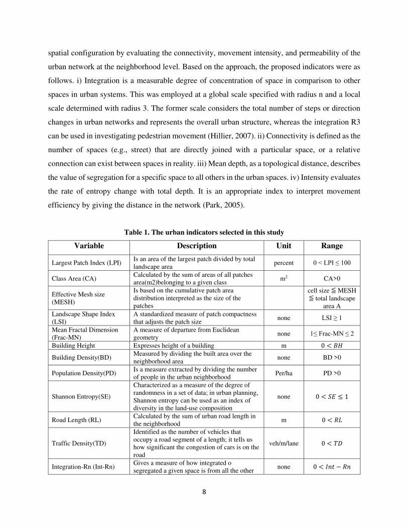
Table 1. The urban indicators selected in this study

Variable Description Unit Range

Largest Patch Index (LPI) Is an area of the largest patch divided by total

landscape area percent 0 < LPI ≤ 100

Class Area (CA) Calculated by the sum of areas of all patches

area(m2)belonging to a given class m2 CA>0

Effective Mesh size

(MESH)

Is based on the cumulative patch area

distribution interpreted as the size of the

patches

cell size ≦ MESH ≦ total landscape

area A

Landscape Shape Index

(LSI)

A standardized measure of patch compactness

that adjusts the patch size none LSI ≥ 1

Mean Fractal Dimension

(Frac-MN)

A measure of departure from Euclidean

geometry none 1≤ Frac-MN ≤ 2

Building Height Expresses height of a building m 0 < 𝐵𝐻

Building Density(BD) Measured by dividing the built area over the

neighborhood area none BD >0

Population Density(PD) Is a measure extracted by dividing the number

of people in the urban neighborhood Per/ha PD >0

Shannon Entropy(SE)

Characterized as a measure of the degree of

randomness in a set of data; in urban planning,

Shannon entropy can be used as an index of

diversity in the land-use composition

none 0 < 𝑆𝐸 ≤ 1

Road Length (RL) Calculated by the sum of urban road length in

the neighborhood m 0 < 𝑅𝐿

Traffic Density(TD)

Identified as the number of vehicles that

occupy a road segment of a length; it tells us

how significant the congestion of cars is on the

road

veh/m/lane 0 < 𝑇𝐷

Integration-Rn (Int-Rn) Gives a measure of how integrated o

segregated a given space is from all the other none 0 < 𝐼𝑛𝑡 − 𝑅𝑛

9

lines of the urban spaces; the highest value is

identified as a busier and integrated the road in

the urban grid (urban core)

Integration-R3(Int-R3)

Calculated by a radius in the local urban

system; R3 is obtained as a function of the

minimum axial line in the urban system that

must travel to the target point

none 0 < 𝐼𝑛𝑡 − 𝑅3

Mean depth(MD)

Displays distance between space topologically;

it calculates the distance between each axial

line and all the others; the deepest axial lines

are farthest ones

none 0 < 𝑀𝐷

Intensity (I)

In a spatial network, intensity calculates the

rate of change of entropy with total depth;

intensity is an appropriate index to interpret

movement efficiency by giving the distance in

the network

none 0 < 𝐼

Connectivity Measures the number of immediate neighbors

that are directly connected to space none 0 < 𝐼

2.3. Methodology

2.3.1 The PCA implementation: Considering a large number of variables (16 indicators) applied

in the current work and also the possibility of the internal relationship between the variables

affecting LST in the study areas, the PCA method was used in the first step. As a pre-analysis step,

PCA is an exploratory technique to obtain important variables in the form of components by

dimensionality-reduction method (Jolliffe & Cadima, 2016). PCA includes the following equation: 𝑝𝑐𝑖𝑗 = ∑ 𝑋𝑖𝑘𝐸𝑘𝑗𝑛𝑘=1

where pcij is the component score of the jth principal component for cell i, Xik is the value of the

kth layer for cell i, and Ekj is the element of the eigenvector matrix at row k and column j (Yue,

Liu, Fan, Ye, & Wu, 2012). before PCA, the numeric datasets were standardized using the standard

deviations, providing the dimensionless variables with unit variance and standard deviation.

2.3.2 OLS analysis: Traditionally, OLS is a multiple regression analysis based on spatially

constant features of the dependent and independent variables within the study area (S. Li et al.,

2010). Generally, it suites the various datasets and could be applied equally across the whole study

area (Tian, Qiu, Yang, Xiong, & Wang, 2012). According to the assumption of observation

independence, OLS would be failed when applied to the spatial data referring to the geo-referenced

data. OLS model can be written as (Luo & Peng, 2016): 𝛾𝑖 = 𝛽0 + ∑ 𝛽𝑘𝑘 𝑥𝑖𝑘 + 𝜀𝑖

10

where yi=1,2,…n represents the dependent variable, xk (k= 1,2,…M) represents the explanatory

variable, β0 is the intercept, βk is the regression coefficient, and ε stands for the random error. In

the present study, applying the OLS regression model, the nature of relationships between the

underlying factors and LST was found, directly allowing to compare the findings with GWR.

2.3.3 GWR analysis: Since the observed geographical and ecological patterns had been

investigated in this paper, the GWR regression model was tested to produce prediction and

parameter estimates at the neighborhood scale effectively. Mathematically, the GWR model takes

the following form (C. Zhao et al., 2018): 𝛾𝑖 = 𝛽0(𝑢𝑖 ,𝑣𝑖) + ∑ 𝛽𝑘𝑘 (𝑢𝑖 ,𝑣𝑖)𝑥𝑖𝑘 + 𝜀𝑖

Where (𝑢𝑖 ,𝑣𝑖) indicates the geographic location of each neighborhood (i), β0(ui,vi) is the

geographically varying intercept, βk(ui, vi) represents the local coefficients estimated for the

explanatory variable xk at the point i,. Also, εi is the random error at point i with distribution N

(Luo & Peng, 2016).

2.3.4 Efficiency assessment of the OLS and GWR model: GWR is an extended version of OLS

that, in collaboration with it, provides powerful statistical tools to evaluate variation in the

association among variables. To highlight the efficiency of two conducted model concerning the

goodness-of-fit and residual spatial autocorrelation, the obtained results were compared in this

study by applying some indices, such as the coefficient of determination (R2), the global Moran's

I index (Moran's I), and the corrected Akaike Information Criterion (AICc)(S. Li et al., 2010; Xiao

et al., 2013; C. Zhao et al., 2018).

The coefficient of determination (R2) is a value to measure the model fitness, computed to reflect

the relationship of each explanatory variable. By a comparison between the predicted values at

each regression point and the observed values, the higher R2 could be used to indicate better

performance and stronger predictive ability of two conducted models (Propastin, 2009).

Additionally, two main performance indicators, including the global Moran's I and the corrected

Akaike Information Criterion (AICc), were tested in this study. Comparing the results, AICc is an

important value to assess fit for both the GWR and OLS model's performance. In general, the best

model is determined by lower AICc, indicating a closer approximation of the model to reality (Tian

et al., 2012). Also, the global Moran's I is a clustering analysis statistic able to calculate the spatial

autocorrelation of the residuals based on feature location and value, ranging from -1 to 1. The

11

model will be superior if the distribution of the residuals obtained from the regression model tends

to be dispersed. In other words, the lower Moran's I suggest more random spatial patterns in the

residuals by the best model. When using the spatial regression models, the residuals obtained from

fitting the models must be locally independent of each other; hence an autocorrelation coefficient

is used to test the spatial dependence of the standard deviation of the residual (std-residual),

obtained from OLS and GWR models.

3. Results

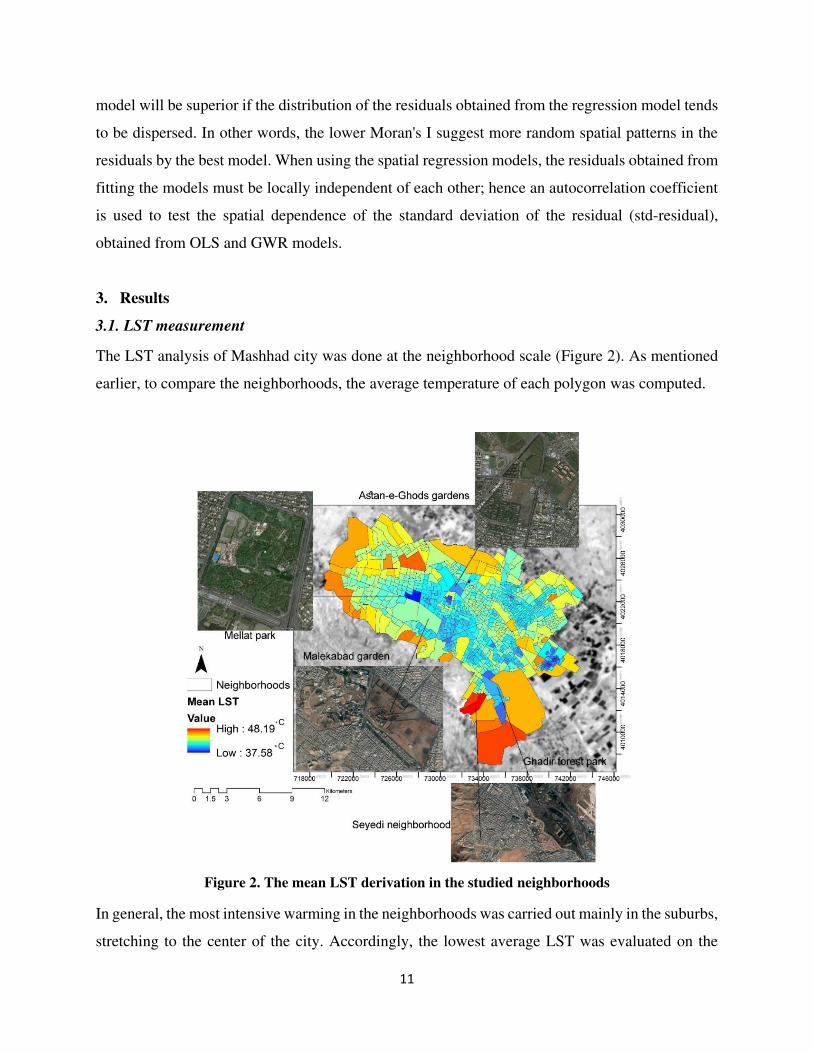
3.1. LST measurement

The LST analysis of Mashhad city was done at the neighborhood scale (Figure 2). As mentioned

earlier, to compare the neighborhoods, the average temperature of each polygon was computed.

Figure 2. The mean LST derivation in the studied neighborhoods

In general, the most intensive warming in the neighborhoods was carried out mainly in the suburbs,

stretching to the center of the city. Accordingly, the lowest average LST was evaluated on the

12

Mellat park neighborhood (37.58 °C) in the west of Mashhad, where most parts of the area were

fully covered with the shadows of trees and shrubs. In contrast, the highest surface temperature

was 48.19 °C in the Seyedi neighborhood, where residential buildings with small areas of green

spaces have mainly formed the structure of the neighborhood in the south-eastern of the city.

Overall, the results demonstrated that the neighborhoods within the urban center had a relatively

lower temperature than those in the suburbs due to an abundance of green space and gardens, in

particular, Astan-e-Ghods gardens like Malekabad and Imam Reza with 42.4 °C and 41.04 °C

average temperatures, respectively. Exceptionally, some neighborhoods had higher temperatures

than others due to adjacent land use types like Mashhad railway station with an average

temperature of 45.41 °C or being affected by the exposed solar radiation, mainly located around

the holy shrine (43.51 °C).

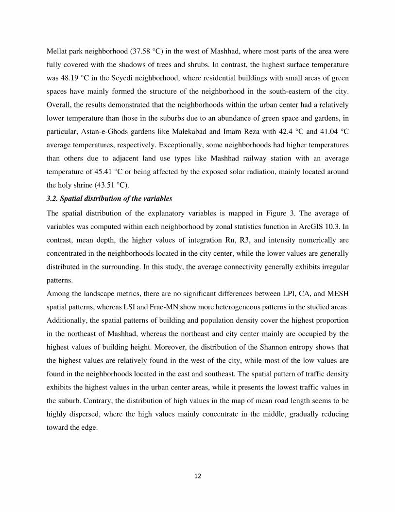
3.2. Spatial distribution of the variables

The spatial distribution of the explanatory variables is mapped in Figure 3. The average of

variables was computed within each neighborhood by zonal statistics function in ArcGIS 10.3. In

contrast, mean depth, the higher values of integration Rn, R3, and intensity numerically are

concentrated in the neighborhoods located in the city center, while the lower values are generally

distributed in the surrounding. In this study, the average connectivity generally exhibits irregular

patterns.

Among the landscape metrics, there are no significant differences between LPI, CA, and MESH

spatial patterns, whereas LSI and Frac-MN show more heterogeneous patterns in the studied areas.

Additionally, the spatial patterns of building and population density cover the highest proportion

in the northeast of Mashhad, whereas the northeast and city center mainly are occupied by the

highest values of building height. Moreover, the distribution of the Shannon entropy shows that

the highest values are relatively found in the west of the city, while most of the low values are

found in the neighborhoods located in the east and southeast. The spatial pattern of traffic density

exhibits the highest values in the urban center areas, while it presents the lowest traffic values in

the suburb. Contrary, the distribution of high values in the map of mean road length seems to be

highly dispersed, where the high values mainly concentrate in the middle, gradually reducing

toward the edge.

13

Figure 3. Spatial distribution of the variables. a-e: the variables of urban spatial configurations; f-j:

the metrics of landscape structure; k-n: the morphological variables and, o-p: the traffic and road

features.

3.3. Calculation of PCA

Among the 16 mentioned variables, five principal components (PCs) were identified using the Cut-

Off point of the Scree plot and the eigenvalues higher than 1. Table 2 provides the eigenvalues and

percentages of the explained variance of the selected components. Also, the first five principal

components exhibited the highest variance in the original data using the proportion of variance

explained (PVE). Accordingly, the PCs determined 86.2% of the variability by cumulative percent

variance.

14

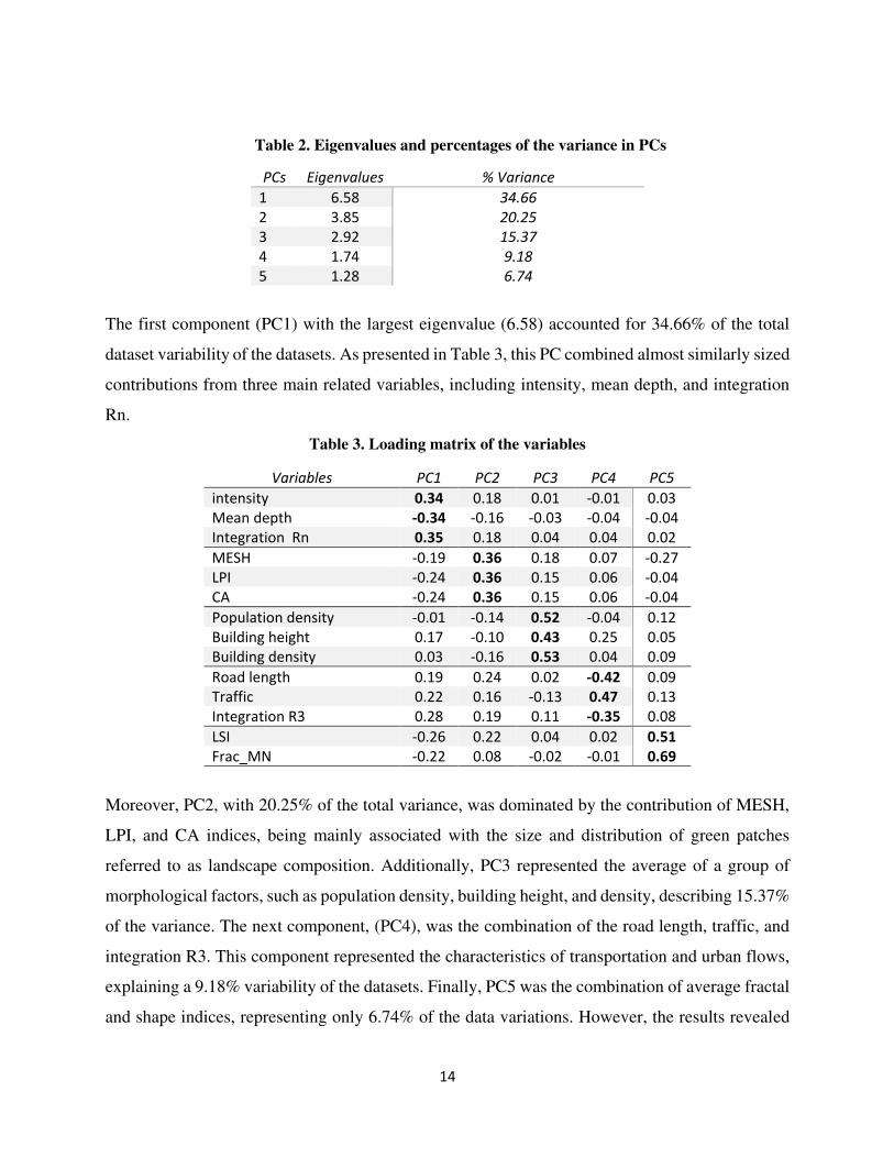
Table 2. Eigenvalues and percentages of the variance in PCs

% Variance Eigenvalues PCs

34.66 6.58 1

20.25 3.85 2

15.37 2.92 3

9.18 1.74 4

6.74 1.28 5

The first component (PC1) with the largest eigenvalue (6.58) accounted for 34.66% of the total

dataset variability of the datasets. As presented in Table 3, this PC combined almost similarly sized

contributions from three main related variables, including intensity, mean depth, and integration

Rn.

Table 3. Loading matrix of the variables

PC5 PC4 PC3 PC2 PC1 Variables

0.03 -0.01 0.01 0.18 0.34 intensity

-0.04 -0.04 -0.03 -0.16 -0.34 Mean depth

0.02 0.04 0.04 0.18 0.35 Integration Rn

-0.27 0.07 0.18 0.36 -0.19 MESH

-0.04 0.06 0.15 0.36 -0.24 LPI

-0.04 0.06 0.15 0.36 -0.24 CA

0.12 -0.04 0.52 -0.14 -0.01 Population density

0.05 0.25 0.43 -0.10 0.17 Building height

0.09 0.04 0.53 -0.16 0.03 Building density

0.09 -0.42 0.02 0.24 0.19 Road length

0.13 0.47 -0.13 0.16 0.22 Traffic

0.08 -0.35 0.11 0.19 0.28 Integration R3

0.51 0.02 0.04 0.22 -0.26 LSI

0.69 -0.01 -0.02 0.08 -0.22 Frac_MN

Moreover, PC2, with 20.25% of the total variance, was dominated by the contribution of MESH,

LPI, and CA indices, being mainly associated with the size and distribution of green patches

referred to as landscape composition. Additionally, PC3 represented the average of a group of

morphological factors, such as population density, building height, and density, describing 15.37%

of the variance. The next component, (PC4), was the combination of the road length, traffic, and

integration R3. This component represented the characteristics of transportation and urban flows,

explaining a 9.18% variability of the datasets. Finally, PC5 was the combination of average fractal

and shape indices, representing only 6.74% of the data variations. However, the results revealed

15

that connectivity and entropy had no significant contributions to the principal components among

the variables.

3.4. The relationship establishment between LST and the components using OLS and GWR

model.

In this section, the relationship between the PCs and LST was established using the OLS and GWR

models. The OLS model was first adopted to assess the global statistical relationship between the

dependent (LST) and independent variables (PCs). Furthermore, the corresponding GWR model

was used to investigate the non-stationary spatial relationships between the dependent variable and

the components in the OLS model. A summary of the results in both OLS and GWR models is

presented in Table 4.

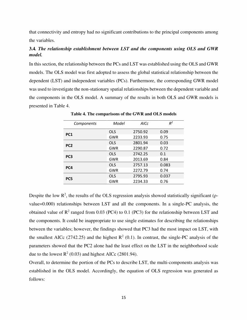
Table 4. The comparisons of the GWR and OLS models

Components Model AICc R2

PC1 OLS 2750.92 0.09

GWR 2233.93 0.75

PC2 OLS 2801.94 0.03

GWR 2290.87 0.72

PC3 OLS 2742.25 0.1

GWR 2013.69 0.84

PC4 OLS 2757.13 0.083

GWR 2272.79 0.74

PC5 OLS 2795.93 0.037

GWR 2234.33 0.76

Despite the low R2, the results of the OLS regression analysis showed statistically significant (ρ-

value=0.000) relationships between LST and all the components. In a single-PC analysis, the

obtained value of R2 ranged from 0.03 (PC4) to 0.1 (PC3) for the relationship between LST and

the components. It could be inappropriate to use single estimates for describing the relationships

between the variables; however, the findings showed that PC3 had the most impact on LST, with

the smallest AICc (2742.25) and the highest R2 (0.1). In contrast, the single-PC analysis of the

parameters showed that the PC2 alone had the least effect on the LST in the neighborhood scale

due to the lowest R2 (0.03) and highest AICc (2801.94).

Overall, to determine the portion of the PCs to describe LST, the multi-components analysis was

established in the OLS model. Accordingly, the equation of OLS regression was generated as

follows:

16

𝐿𝑆𝑇 = 41.91 − 0.17(𝑃𝐶1) − 0.14(𝑃𝐶2) − 0.27(𝑃𝐶3) + 0.31(𝑃𝐶4) − 0.22(𝑃𝐶5)

Where the value of R equals 0.58, and the overall goodness-of-fit (R2) is 0.34, indicating that these

PCs help to explain the LST distribution with a confidence level of 34%. In the equation, also, the

number 41.91 is identified as the fixed coefficient which is used to predict LST. Furthermore,

multi-components analysis denotes the degree of the PC effect on decreasing and increasing the

LST. It was observed that PC4 was the only independent variable with a positive influence,

whereas the other components all had a negative impact. This PC corresponds closely to the

physical properties of street geometry, pavements plus their colors, traffic density, and activities

in the urban neighborhoods. Therefore, the average of LST would be positively increased to 0.318-

point when PC4 is grown 1-point statistically. Based on the equation, PC2 involved in the

composition features of urban green patches had the lowest fixed coefficient on LST changes,

where an increase in PC2 is associated with a decrease in LST up to 0.14 degrees.

To compare the models, the results of the GWR model are listed in Table 4. Accordingly, the

strength of the relationships between the five predictors (PCs) and LST boosted significantly. Also,

single-PC analysis reflected better performance than the OLS model by a relatively smaller

measure of AICc and a higher value of R2. Similar to the OLS model, PC3 was identified as the

most important factor in LST variations by the highest values of R2 (0.84) and the lowest AICc

(2013.69), whereas PC2 exhibited a weak impact on the LST due to the minimum R2 (0.72) and

maximum AICc (2801.94). Therefore, the sign of the regression coefficients of the PCs in two

conducted models suggesting the morphological aspects of the neighborhoods had the strongest

effects on LST variations, where an increase in the building height and population density are

associated with decreases in the average of LST at the neighborhood level. On the contrary, PC2

showed the area, size, and continuity of green patches to have the least effect on reducing the

average of LST in neighborhoods.

3.5. Assessment of the models' efficiency

To evaluate the efficiency of both applied models, the estimated LST maps were represented using

OLS and GWR models (Figure 4). Overall, the spatial patterns of the LST generated by the models

showed a similar trend and goodness of fit with the original map.

17

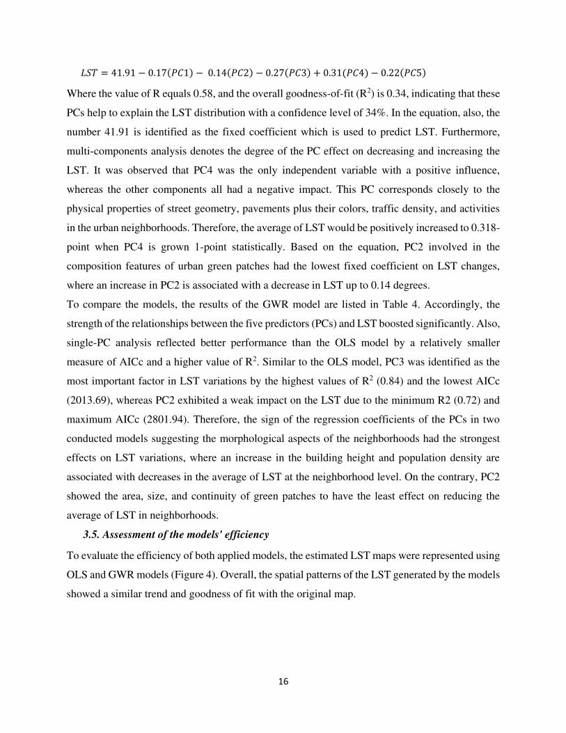
Figure 4. Predicted LST map obtained from GWR model (left), and estimated LST map generated

from OLS model (right)

The predicted map usually is characterized by LST higher values concentrated in the suburbs and

lower values located mostly in the neighborhoods in the city center. Additionally, it can be seen

that the minimum and maximum of predicted values are beyond the observed data. However, these

indicate that the findings reflect changes in variables and highlight a much detailed spatial

distribution of LST. A noticeable difference is that the generated maps indicate more variations in

the neighborhoods situated in the east and northwestern of the city, where the higher values of LST

happen mostly in developing neighborhoods with extensive bare lands, high scattered built areas,

and insufficient UGS.

Moreover, the corresponding results of the models are statistically compared by describing data

variations and addressing spatial autocorrelation. Since the model is non-stationary, the GWR

model computes the predicted values well for spatial differentiation in the neighborhoods. As

presented in Table 5, the coefficient of determination (R2) of the OLS model is 0.343, whereas

the R2 for the GWR model is 0.678. Towards a better fitting model, the higher value of R2 is

considered to explain the relationships more efficiently.

Table 5. Performance indicators of GWR and OLS models

Moran’s I AICc R2

Validation indexes

Regression models

0.272 Moran's Index 2503.46 0.343 OLS

0.000 p-value

0.018 Moran's Index 2125.6 0.678 GWR

0.000 p-value

18

This implies that GWR is a powerful model for explaining the LST changes in response to the

underlying components and would extremely enable the findings to fit the observed LST. Also,

the higher R2 suggests that the relationships between LST and the PCs may exhibit spatial non-

stationarity. Moreover, the AICc value for GWR is lower than OLS, with a notable decrease of

more than 377.86 points, being strong evidence for a real improvement in the results based on the

local model (GWR). In addition to the comparisons mentioned above, the Moran's I for the GWR

model gives a smaller value (0.018) than the OLS one (0. 272), exhibiting a more random spatial

pattern of residual values in the GWR model. This means the OLS model does not fully explain

the whole datasets due to a violation of normality assumption and hence cannot provide closer

representations of reality than the GWR model. Therefore, these results confirm the efficiency of

GWR over the OLS model, addressing the ability to predict the LST variations and spatial

autocorrelation.

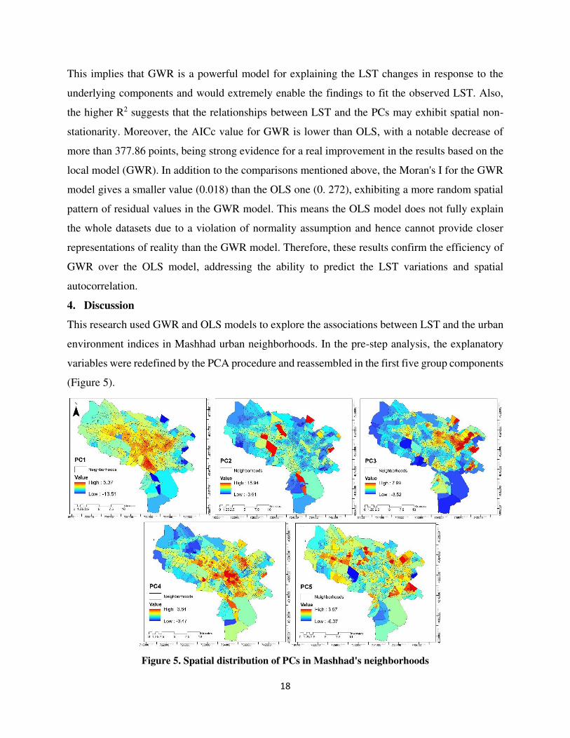
4. Discussion

This research used GWR and OLS models to explore the associations between LST and the urban

environment indices in Mashhad urban neighborhoods. In the pre-step analysis, the explanatory

variables were redefined by the PCA procedure and reassembled in the first five group components

(Figure 5).

Figure 5. Spatial distribution of PCs in Mashhad's neighborhoods

19

In general, the results reported clear connections between LST and PCs at the neighborhood level.

Furthermore, the findings confirmed the regression relationships between LST and PCs to be

identified by significant spatial non-stationarity. The results provided clear evidence that the GWR

model made a significantly better prediction of LST by smaller AICc, higher R2, and the smaller

value of Moran's I compared to the OLS model. The results are discussed in the following parts:

4.1. PC1 and LST

The first component, modeled by intensity, mean depth, and integration Rn, explained 34.66% of

the total variance. Configurationally, the variables contributing to PC1 are mainly dealing with

urban cores, space geometry, road orientation, movements, and land use/ land cover arrangement.

As displayed in Figure 5, the high values of PC1 generally appeared in the neighborhoods

extending from the urban core (in the center) to the west, whereas the low values were distributed

in the suburb. Overall, the results indicated that a lower mean LST was detected in a smaller

neighborhood with higher integrated spaces in comparison to larger neighborhoods and higher

segregated spaces.

Our findings confirmed the LST intensities to be derived via the various configuration of the urban

neighborhoods negatively. Besides PC3 and PC5, PC1 was found to be the most influential

component able to mitigate the LST in two effective ways: internal spatial structure and contiguity

of the neighborhoods. These findings emphasize the role of neighborhood configuration in

representing the internal spatial structure with maximum integration and intensity, thereby holding

the various parts of a neighborhood constant. On the contrary, neighborhoods with low

configurational attributes do not have a coherent internal structure, being identified with the

dispersed distribution. Moreover, spatial configuration widely organizes the arrangement of urban

land use, spatial patterns of land cover, and structure of urban morphology in the small

neighborhoods that tend to have more compact urban clusters, larger contiguity of integrated cores

with medium and high-rise buildings, and interconnected spaces. Hence, the clustered built-up

neighborhoods may have a more suitable urban canopy to reduce direct sunlight and consequently

the LST effect as it is closely related to airflow and the city's ventilation conditions. Indeed, the

spatial configuration can optimize high-rise building arrangement and street layout around the

integrated spaces to extend shades and urban canopies. Therefore, it is comprehensible that the

spatial configuration can qualitatively improve interaction with cooler airflow and cause the

mitigation of LST. Although contradictory results have been reported in some cases (Coutts,

20

Beringer, & Tapper, 2007; Schwarz, 2010; Yue et al., 2019), our findings are in agreement with

previous work (Lan & Zhan, 2017; Soltanifard & Aliabadi, 2019; Yin, Yuan, Lu, Huang, & Liu,

2018). Differences in approach, statistical methods, and climatic characteristics may be

contributing to these inconsistencies in the results.

4.2. PC2 and LST

The starting point to assess the landscape structure in the studied areas was to investigate the spatial

patterns of the green spaces in terms of landscape composition and configuration. However,

MESH, LPI, and CA were the main contributors of PC2, which were summarized as the LST

predictors by the PC analysis method. As shown in Figure 5, higher values of the component

tended to be included in the major green spaces and private gardens, such as Mellat park, Ghadir

forest park, Malekabad, and Astan-e-Ghods gardens (Figure 2). Although our analysis showed that

most studied neighborhoods met a fragmented pattern of the green patches, the regression analysis

significantly indicated an inverse relationship between PC2 and LST. To explain the relationship,

CA and LPI values should be relatively considered in the area of each neighborhood. Accordingly,

the subtractive trend of LPI, CA, and MESH in the small neighborhoods thoroughly supported the

aggregative and more connected patches that provide dense green spaces. Therefore, the results

demonstrated that large and continuous patches provided higher cooling effects than those of the

larger neighborhoods with the same fragmented green spaces or disconnected patches. Our results

are supported by the reported studies (Amani-Beni, Zhang, Xie, & Shi, 2019; Cao, Onishi, Chen,

& Imura, 2010; J. Song, Du, Feng, & Guo, 2014).

4.3. PC3 and LST

Based on the relationship between PCA’s and LST, PCA3 has the strongest effect on the average

LST among other components. Building height, building density, and population density were

three main contributors to PC3, describing the morphological characteristics of neighborhoods.

Figure 5 illustrated the spatial patterns of PC3, high values are distributed in the center and north

of the city, in contrast to the suburban areas with the lowest building and population density. In

general, as a combined factor, PC3 has a negative influence on the mean LST, where LST is

intensified in a neighborhood with low building and population density. Several empirical studies

have reported the relationship between the characteristics of urban morphology and LST in various

ways (Guo, Zhou, Wu, Xiao, & Chen, 2016; Jin, Cui, Wong, & Ignatius, 2018). However, we

found the negative effect of the results to be related to building height and clusters with shadows,

21

where increasing height and density could mitigate LST even during the strong sunlight and

heating influence. Our results are corroborated by some studies (Cai, Ren, Xu, Lau, & Wang, 2018;

Jin et al., 2018; Scarano & Mancini, 2017; Sun, Gao, Li, Wang, & Liu, 2019).

4.4. PC4 and LST

In the current work, PC4 was another responsible component for explaining the variance of LST

at the neighborhood level. The component had a heavy loading matrix with road length, integration

R3, and traffic density, indicating the transportation features of the urban network. The results

showed that PC4 positively correlated with the average LST. Due to the fundamental

transportation elements, such as traffic, street features, and movement patterns, indeed, the

complex transportation network forms components of urban structure and its associations from the

scale of settlements to the scale of the street block (Marshall, 2005). Given the main contribution

of transportation elements to urban structure features, several studies confirm the role of

transportation to alter the behavior of LST patterns significantly (Giridharan, Lau, Ganesan, &

Givoni, 2007; Lee, Moon, Choi, & Yoon, 2018; Oke, 1988). Based on the findings, the increasing

trend of LST directly is related to an effective decrease in surface albedo, in particular, the

impervious surfaces, including streets and pedestrian road pavements. Moreover, land use, urban

space geometry, and road construction affect traffic density in the neighborhoods, outlining the

heat behavior along with both road and land use types. Accordingly, the increased input of

anthropogenic heat and street surface type causes heating emission of the road to the urban

environment and increases LST. These results are confirmed by previous studies (Chapman,

Thornes, & Bradley, 2001; Oke, 1988; Walawender, Szymanowski, Hajto, & Bokwa, 2014).

4.5. PC5 and LST

In this study, the PC5 is characterized by the shape (LSI) and the complexity of the green patches

(Frac-MN), referred to as the configuration features at the neighborhood level. Figure 5 presents

the distribution of the component with an important role in describing the LST variation.

Routinely, UGS properties are the distinctive predictors of the LST in the urban environment;

however, more debates have remained on the composition and configuration effects of UGS on

LST. The results strongly indicate PC5, compared to PC2, to be a better predictor for estimating

the changes of LST. Although, all the measures of LSI and Frac-MN have similar trends in general,

with the low values in the center and the scattered high values irregularly in a few cases, a

combination of two factors (PC5) has a negative effect on LST unexpectedly. In a single analysis,

22

the neighborhoods with the larger average of Frac-MN and LSI provide a greater connection

between the patches and surrounding, facilitating energy transmission efficiency. Besides, the

decreasing trend of both factors should be simultaneously considered with LPI and CA directions

in the studied neighborhoods. The neighborhoods with the minimum of LSI, Frac-MN, LPI, and

CA, which are mainly concentrated in the center, spatially show more fragmented and isolated

green patches. As proven in previous studies (Amani-Beni et al., 2019; X. Zhang, Zhong, Feng, &

Wang, 2009), an increase in the fragmentation of green patches leads to a positive effect in LST;

however, the simultaneous impacts of the components is negative on LST. Unlike the

neighborhoods in the suburbs, the results reflect that the high aggregation and density of the green

patches in the neighborhoods could mitigate heat intensities by representing a higher cooling

function. These suggest that less complexity and shape of the green patches may better regulate

LST interestingly. The results of the present work are consistent with those of several previous

studies (Connors, Galletti, & Chow, 2013; Dugord, Lauf, Schuster, & Kleinschmit, 2014; Peng et

al., 2011; Xie, Wang, Chang, Fu, & Ye, 2013; Zhou, Huang, & Cadenasso, 2011).

5. Conclusion

In summary, the present work thoroughly highlights the following major findings:

First, as regards the LST trends, urban neighborhoods increasingly showed distinct LST changes

from the center to the suburb, affected by urban configuration, morphology, roads, traffic, as well

as landscape composition and configuration.

Second, all explanatory variables demonstrated a significant contribution to LST intensities. The

morphological features of neighborhoods (PC3) had the most negative influence on LST. In

contrast, the landscape composition of the green patches(PC2) exhibited the lowest negative

impacts on LST changes. Furthermore, road and traffic characteristics of the neighborhoods (PC4)

were the only effective components to alert the average LST positively. Therefore, our empirical

results suggested developing high-rise buildings to provide shading during days, besides

increasing urban trees and vegetation to produce the cooling effect.

Third, this study confirmed that, compared to the OLS model, the GWR model had an excellent

ability to detect the scale-dependence of the relationships between the LST and the components,

especially in heterogeneous regions. Hence, for urban policymakers, the GWR model may be

suitable assistance to determine the most reliable action plan at the neighborhood level.

23

Finally, although removing the hot and impervious surfaces is impossible, urban planners and

designers can mitigate heat effects by reforming urban morphological context, improving planting

quality, and redesigning urban configuration. In particular, for developing countries, like Iran, it is

suggested to pay more attention to the arrangement of buildings, the configuration of green spaces,

and the enhancement of the urban spatial configuration at the neighborhood level as effective

strategies to create a comfortable outdoor environment, alleviating LST and corresponding adverse

effects. This study presents findings that are of major significance to climate experts, urban and

regional planners, environmentalists, and policymakers to explore measures for mitigating

uncontrolled urban expansion and thermal discomfort in Mashhad City. This caters to the vision

of the United Nations Sustainable Development Goals (SDGs) for sustainable cities and

communities (SDG 11), and good health and wellbeing (SDG 3) and Take urgent action to combat

climate change and its impacts ( SDG 13) by 2030.

24

Declarations

Conflict of Interest: The authors have no conflicts of interest to declare that are relevant to the

content of this article.

Funding Statement: The authors did not receive support from any organization for the

submitted work.

Author's Contribution: All authors contributed to the study's conception and design. Material

preparation, data collection, and analysis were performed by Hadi Soltanifard, Abdolreza

Kashki, and Mokhtar Karami. The first draft of the manuscript was written by Hadi Soltanifard

and all authors commented on previous versions of the manuscript. All authors read and

approved the final manuscript.

Availability of data and material: Not Applicable

Code availability: Not Applicable

Ethics approval: Not Applicable

Consent to participate: Not Applicable

Consent for publication: All Authors consent to the publication of the article after acceptance.

Reference

Akbari, H. (2007). Opportunities for Saving Energy and Improving Air Quality in Urban Heat

Islands. Advances in Passive Cooling, 30.

Ali-Toudert, F., & Mayer, H. (2006). Numerical study on the effects of aspect ratio and

orientation of an urban street canyon on outdoor thermal comfort in a hot and dry climate.

Building and Environment, 41(2), 94–108.

Alobaydi, D., Bakarman, M. A., & Obeidat, B. (2016). The Impact of Urban Form Configuration

on the Urban Heat Island: The Case Study of Baghdad, Iraq. Procedia Engineering, 145,

820–827. https://doi.org/10.1016/j.proeng.2016.04.107

Amani-Beni, M., Zhang, B., Xie, G.-D., & Shi, Y. (2019). Impacts of urban green landscape

patterns on land surface temperature: Evidence from the adjacent area of Olympic Forest

Park of Beijing, China. Sustainability, 11(2), 513.

Avdan, U., & Jovanovska, G. (2016). Algorithm for automated mapping of the land surface

temperature using LANDSAT 8 satellite data. Journal of Sensors, 2016.

25

Barsi, J. A., Schott, J. R., Hook, S. J., Raqueno, N. G., Markham, B. L., & Radocinski, R. G.

(2014). Landsat-8 thermal infrared sensor (TIRS) vicarious radiometric calibration. Remote

Sensing, 6(11), 11607–11626.

Brown, S., Versace, V. L., Laurenson, L., Ierodiaconou, D., Fawcett, J., & Salzman, S. (2012).

Assessment of spatiotemporal varying relationships between rainfall, land cover, and

surface water area using geographically weighted regression. Environmental Modeling &

Assessment, 17(3), 241–254.

Brunsdon, C., Fotheringham, A. S., & Charlton, M. E. (1996). Geographically weighted

regression: a method for exploring spatial nonstationarity. Geographical Analysis, 28(4),

281–298.

Cai, M., Ren, C., Xu, Y., Lau, K. K.-L., & Wang, R. (2018). Investigating the relationship

between local climate zone and land surface temperature using an improved WUDAPT

methodology--A case study of Yangtze River Delta, China. Urban Climate, 24, 485–502.

Cao, X., Onishi, A., Chen, J., & Imura, H. (2010). Quantifying the cool island intensity of urban

parks using ASTER and IKONOS data. Landscape and Urban Planning, 96(4), 224–231.

Carnielo, E., & Zinzi, M. (2013). Optical and thermal characterization of cool asphalts to

mitigate urban temperatures and building cooling demand. Building and Environment, 60,

56–65.

Chapman, L., Thornes, J. E., & Bradley, A. V. (2001). Modeling of road surface temperature

from a geographical parameter database. Part 2: Numerical. Meteorological Applications,

8(4), 421–436.

Connors, J. P., Galletti, C. S., & Chow, W. T. L. (2013). Landscape configuration and urban heat

island effects: Assessing the relationship between landscape characteristics and land surface

temperature in Phoenix, Arizona. Landscape Ecology, 28(2), 271–283.

https://doi.org/10.1007/s10980-012-9833-1

Coutts, A. M., Beringer, J., & Tapper, N. J. (2007). Impact of increasing urban density on local

climate: spatial and temporal variations in the surface energy balance in Melbourne,

Australia. Journal of Applied Meteorology and Climatology, 46(4), 477–493.

26

Dugord, P.-A., Lauf, S., Schuster, C., & Kleinschmit, B. (2014). Land use patterns, temperature

distribution, and potential heat stress risk--the case study Berlin, Germany. Computers,

Environment and Urban Systems, 48, 86–98.

Eleftheriou, D., Kiachidis, K., Kalmintzis, G., Kalea, A., Bantasis, C., Koumadoraki, P., …

Gemitzi, A. (2018). Determination of annual and seasonal daytime and nighttime trends of

MODIS LST over Greece-climate change implications. Science of the Total Environment,

616, 937–947.

Fallmann, J., Forkel, R., & Emeis, S. (2016). Secondary effects of urban heat island mitigation

measures on air quality. Atmospheric Environment, 125, 199–211.

Ferreira, L. S., Helena, D., & Duarte, S. (2019). Urban Climate Exploring the relationship

between urban form, land surface temperature, and vegetation indices in a subtropical

megacity. Urban Climate, 27(July 2018), 105–123.

https://doi.org/10.1016/j.uclim.2018.11.002

Fotheringham, A. S., Brunsdon, C., & Charlton, M. (2003). Geographically weighted regression:

the analysis of spatially varying relationships. John Wiley & Sons.

Giridharan, R., Lau, S. S. Y., Ganesan, S., & Givoni, B. (2007). Urban design factors influencing

heat island intensity in high-rise high-density environments of Hong Kong. Building and

Environment, 42(10), 3669–3684.

Guo, G., Zhou, X., Wu, Z., Xiao, R., & Chen, Y. (2016). Characterizing the impact of urban

morphology heterogeneity on land surface temperature in Guangzhou, China.

Environmental Modelling & Software, 84, 427–439.

Han-qiu, X., & Ben-qing, C. (2004). Remote sensing of the urban heat island and its changes in

the Xiamen City of SE China. Journal of Environmental Sciences, 16(2), 276–281.

Harris, P., Fotheringham, A. S., Crespo, R., & Charlton, M. (2010). The use of geographically

weighted regression for spatial prediction: an evaluation of models using simulated data

sets. Mathematical Geosciences, 42(6), 657–680.

Hillier, B. (2007). Space is the machine: a configurational theory of architecture. London: space

syntax, UCL University Press.

27

Hirano, Y., & Fujita, T. (2012). Evaluation of the impact of the urban heat island on residential

and commercial energy consumption in Tokyo. Energy, 37(1), 371–383.

Huang, C., Barnett, A. G., Wang, X., Vaneckova, P., FitzGerald, G., & Tong, S. (2011).

Projecting future heat-related mortality under climate change scenarios: a systematic

review. Environmental Health Perspectives, 119(12), 1681–1690.

Huang, G., Zhou, W., & Cadenasso, M. L. (2010). Understanding the relationship between urban

land surface temperature, landscape heterogeneity, and social structure. 2010 IEEE

International Geoscience and Remote Sensing Symposium, 3933–3936.

Huang, Y., Yuan, M., & Lu, Y. (2019). Spatially varying relationships between surface urban

heat islands and driving factors across cities in China. Environment and Planning B: Urban

Analytics and City Science, 46(2), 377–394.

Jin, H., Cui, P., Wong, N. H., & Ignatius, M. (2018). Assessing the Effects of Urban Morphology

Parameters on Microclimate in Singapore to Control the Urban Heat Island Effect.

Sustainability, 10(206). https://doi.org/10.3390/su10010206

Johansson, E. (2006). Influence of urban geometry on outdoor thermal comfort in a hot dry

climate: A study in Fez, Morocco. Building and Environment, 41(10), 1326–1338.

Jolliffe, I. T., & Cadima, J. (2016). Principal component analysis: a review and recent

developments. Philosophical Transactions of the Royal Society A: Mathematical, Physical

and Engineering Sciences, 374(2065), 20150202.

Kalota, D. (2017). Exploring the relation of land surface temperature with selected variables

using geographically weighted regression and ordinary least square methods in Manipur

State, India. Geocarto International, 32(10), 1105–1119.

Krafta, R. (1997). Urban Configurational Complexity Definition and Measurement. Space Syntax

First International Symposium, 11. London: space syntax, UCL University Press.

Lan, Y., & Zhan, Q. (2017). How do urban buildings impact summer air temperature? The

effects of building configurations in space and time. Building and Environment, 125, 88–98.

Lee, S., Moon, H., Choi, Y., & Yoon, D. K. (2018). Analyzing Thermal Characteristics of Urban

28

Streets Using a Thermal Imaging Camera : A Case Study on Commercial Streets in Seoul,

Korea. Sustainability, 10(519), 1–21. https://doi.org/10.3390/su10020519

Li, H., Meier, F., Lee, X., Chakraborty, T., Liu, J., Schaap, M., & Sodoudi, S. (2018). Interaction

between urban heat island and urban pollution island during summer in Berlin. Science of

the Total Environment, 636, 818–828.

Li, S., Zhao, Z., Miaomiao, X., & Wang, Y. (2010). Investigating spatial non-stationary and

scale-dependent relationships between urban surface temperature and environmental factors

using geographically weighted regression. Environmental Modelling & Software, 25(12),

1789–1800.

Luo, X., & Peng, Y. (2016). Scale effects of the relationships between urban heat islands and

impact factors based on a geographically-weighted regression model. Remote Sensing, 8(9),

760.

Madrigano, J., Ito, K., Johnson, S., Kinney, P. L., & Matte, T. (2015). A case-only study of

vulnerability to heat wave--related mortality in New York City (2000--2011).

Environmental Health Perspectives, 123(7), 672–678.

Marshall, S. (2005). STREETS & PATTERNS (first). London and New York: Spon Press.

McGarigal, K., & Turner, M. G. (2001). Landscape Metrics for Categorical Map Patterns.

Ndetto, E. L., & Matzarakis, A. (2013). Effects of urban configuration on human thermal

conditions in a typical tropical African coastal city. Advances in Meteorology, 2013.

Oke, T. R. (1988). Street design and urban canopy layer climate. Energy and Buildings, 11(1–3),

103–113.

Park, H. T. (2005). Before integration: A critical review of integration measure in space syntax.

Proceedings of the 5th International Space Syntax Symposium, 555–572.

Peng, S., Piao, S., Ciais, P., Friedlingstein, P., Ottle, C., Breon, F.-M., … Myneni, R. B. (2011).

Surface urban heat island across 419 global big cities. Environmental Science &

Technology, 46(2), 696–703.

Propastin, P. A. (2009). Spatial non-stationarity and scale-dependency of prediction accuracy in

29

the remote estimation of LAI over tropical rainforest in Sulawesi, Indonesia. Remote

Sensing of Environment, 113(10), 2234–2242.

Pu, R., Gong, P., Michishita, R., & Sasagawa, T. (2006). Assessment of multi-resolution and

multi-sensor data for urban surface temperature retrieval. Remote Sensing of Environment,

104(2), 211–225.

Riitters, K., Vogt, P., Soille, P., & Estreguil, C. (2009). Landscape patterns from mathematical

morphology on maps with contagion. Landscape Ecology, 24(5), 699–709.

https://doi.org/10.1007/s10980-009-9344-x

Santamouris, M., Cartalis, C., Synnefa, A., & Kolokotsa, D. (2015). On the impact of urban heat

island and global warming on the power demand and electricity consumption of buildings—

A review. Energy and Buildings, 98, 119–124.

Scarano, M., & Mancini, F. (2017). Assessing the relationship between sky view factor and land

surface temperature to the spatial resolution. International Journal of Remote Sensing,

38(23), 6910–6929.

Schwarz, N. (2010). Urban form revisited—Selecting indicators for characterizing European

cities. Landscape and Urban Planning, 96(1), 29–47.

Shaharuddin, A., Noorazuan, M. H., Takeuchi, W., & Noraziah, A. (2014). The effects of urban

heat islands on human comfort: A case of Klang Valley Malaysia. Global Journal on

Advances Pure and Applied Sciences, 2.

Soltanifard, H., & Aliabadi, K. (2019). Impact of urban spatial configuration on land surface

temperature and urban heat islands: a case study of Mashhad, Iran. Theoretical and Applied

Climatology, 137(3–4), 2889–2903.

Song, J., Du, S., Feng, X., & Guo, L. (2014). The relationships between landscape compositions

and land surface temperature: Quantifying their resolution sensitivity with spatial regression

models. Landscape and Urban Planning, 123, 145–157.

https://doi.org/10.1016/j.landurbplan.2013.11.014

Song, Z., Li, R., Qiu, R., Liu, S., Tan, C., Li, Q., … others. (2018). Global land surface

temperature influenced by vegetation cover and PM2. 5 from 2001 to 2016. Remote

30

Sensing, 10(12), 2034.

Su, Y.-F., Foody, G. M., & Cheng, K.-S. (2012). Spatial non-stationarity in the relationships

between land cover and surface temperature in an urban heat island and its impacts on

thermally sensitive populations. Landscape and Urban Planning, 107(2), 172–180.

Sun, Y., Gao, C., Li, J., Wang, R., & Liu, J. (2019). Quantifying the effects of urban form on

land surface temperature in subtropical high-density urban areas using machine learning.

Remote Sensing, 11(8), 959.

Tian, F., Qiu, G. Y., Yang, Y. H., Xiong, Y. J., & Wang, P. (2012). Studies on the relationships

between land surface temperature and environmental factors in an inland river catchment-

based on geographically weighted regression and MODIS data. IEEE Journal of Selected

Topics in Applied Earth Observations and Remote Sensing, 5(3), 687–698.

Walawender, J. P., Szymanowski, M., Hajto, M. J., & Bokwa, A. (2014). Land surface

temperature patterns in the urban agglomeration of Krakow (Poland) derived from Landsat-

7/ETM+ data. Pure and Applied Geophysics, 171(6), 913–940.

Wang, Y., Chau, C. K., Ng, W. Y., & Leung, T. M. (2016). A review on the effects of physical

built environment attributes on enhancing walking and cycling activity levels within

residential neighborhoods. Cities, 50, 1–15. https://doi.org/10.1016/j.cities.2015.08.004

Wang, Z., Fan, C., Zhao, Q., & Myint, S. W. (2020). A Geographically Weighted Regression

Approach to Understanding Urbanization Impacts on Urban Warming and Cooling: A Case

Study of Las Vegas. Remote Sensing, 12(2), 222.

Weng, Q., Fu, P., & Gao, F. (2014). Generating daily land surface temperature at Landsat

resolution by fusing Landsat and MODIS data. Remote Sensing of Environment, 145, 55–

67.

White-Newsome, J. L., Brines, S. J., Brown, D. G., Dvonch, J. T., Gronlund, C. J., Zhang, K., …

O’Neill, M. S. (2013). Validating satellite-derived land surface temperature with in situ

measurements: A public health perspective. Environmental Health Perspectives, 121(8),

925–931.

Xiao, R., Su, S., Wang, J., Zhang, Z., Jiang, D., & Wu, J. (2013). Local spatial modeling of

31

paddy soil-landscape patterns in response to urbanization across the urban agglomeration

around Hangzhou Bay, China. Applied Geography, 39, 158–171.

https://doi.org/10.1016/j.apgeog.2013.01.002

Xie, M., Wang, Y., Chang, Q., Fu, M., & Ye, M. (2013). Assessment of landscape patterns

affecting the land surface temperature in different biophysical gradients in Shenzhen, China.

Urban Ecosystems, 16(4), 871–886.

Yin, C., Yuan, M., Lu, Y., Huang, Y., & Liu, Y. (2018). Effects of urban form on the urban heat

island effect based on the spatial regression model. Science of the Total Environment, 634,

696–704. https://doi.org/10.1016/j.scitotenv.2018.03.350

Yue, W., Liu, X., Zhou, Y., & Liu, Y. (2019). Impacts of urban configuration on urban heat

island : An empirical study in China mega-cities. Science of the Total Environment, 671,

1036–1046. https://doi.org/10.1016/j.scitotenv.2019.03.421

Yue, W., Liu, Y., Fan, P., Ye, X., & Wu, C. (2012). Assessing spatial pattern of urban thermal

environment in Shanghai, China. Stochastic Environmental Research and Risk Assessment,

26(7), 899–911.

Zhang, X., Zhong, T., Feng, X., & Wang, K. (2009). Estimation of the relationship between

vegetation patches and urban land surface temperature with remote sensing. International

Journal of Remote Sensing, 30(8), 2105–2118.

Zhang, Y., Odeh, I. O. A., & Han, C. (2009). Bi-temporal characterization of land surface

temperature in relation to the impervious surface area, NDVI, and NDBI, using sub-pixel

image analysis. International Journal of Applied Earth Observation and Geoinformation,

11(4), 256–264.

Zhao, C., Jensen, J., Weng, Q., & Weaver, R. (2018). A geographically weighted regression

analysis of the underlying factors related to the surface urban heat island phenomenon.

Remote Sensing, 10(9), 1428.

Zhao, G., Dong, J., Liu, J., Zhai, J., Cui, Y., He, T., & Xiao, X. (2017). Different patterns in the

daytime and nighttime thermal effects of urbanization in Beijing-Tianjin-Hebei urban

agglomeration. Remote Sensing, 9(2), 121.

32

Zhou, W., Huang, G., & Cadenasso, M. L. (2011). Does spatial configuration matter?

Understanding the effects of land cover patterns on land surface temperature in urban

landscapes. Landscape and Urban Planning, 102(1), 54–63.

https://doi.org/10.1016/j.landurbplan.2011.03.009