Embed Size (px)
Citation preview

ANALYSIS OF SOME WAX DEPOSITION
EXPERIMENTS IN A CRUDE OIL CARRYING
PIPE
by
ARNE D. HANDAL
THESIS
for the degree
Master of Science
in Computational Science and Engineering
(Master i Anvendt matematikk og Mekanikk)
Faculty of Mathematics and Natural Sciences
University of Oslo
October 2008
Det matematisk- naturvitenskapelige fakultet
Universitetet i Oslo


Analysis of some Wax Deposition Experiments in a
Crude Oil Carrying Pipe
by
Arne Handal


I
Preface
During my bachelor's degree at the University in Bergen I �nished a technical education indrilling and well technology at Bergen Maritime Vgs. In this period I also worked o�shorefor Odfjell Drilling and had a unique opportunity to combine a practical and theoreticalexperience. I realized soon that I had found my niche and decided to specialize in appliedmathematics related to relevant problems in the oil industry. In the spring 2006 I got in contactwith Research Director (StatoilHydro) Ruben Schulkes who is also Professor (2) at UiO. Hesuggested an interesting subject for my thesis and came up with the idea of doing analysisof wax deposition experiments performed by StatoilHydro. I have been privileged with twoimportant mentors, Ruben Schulkes and Professor Arnold Bertelsen. Arnold Bertelsen and hisstrong knowledge in �uid mechanics have been of large importance. Finally, I want to thankDr.ing. Rainer Ho�mann in StatoilHydro and his most kind assistance related to questions Ihave had about the wax experiment performed under his responsibility.
Arne D. HandalTrondheim, August 29, 2008

II

Contents
Contents II
1 Introduction 3
1.1 Wax - Relevance of the Problem . . . . . . . . . . . . . . . . . . . . . . . . . . 3
1.2 Physical Considerations . . . . . . . . . . . . . . . . . . . . . . . . . . . . . . . 3
1.3 Some Earlier Works and Modeling . . . . . . . . . . . . . . . . . . . . . . . . . 5
1.4 About This Work . . . . . . . . . . . . . . . . . . . . . . . . . . . . . . . . . . . 7
2 Heat Transfer 9
2.1 Graetz problem . . . . . . . . . . . . . . . . . . . . . . . . . . . . . . . . . . . . 9
2.1.1 Formulation of the Problem . . . . . . . . . . . . . . . . . . . . . . . . . 9
2.1.2 Solution of the Problem . . . . . . . . . . . . . . . . . . . . . . . . . . . 10
2.1.3 Solving the Coe�cients . . . . . . . . . . . . . . . . . . . . . . . . . . . 12
2.1.4 Dimensionless Temperature Pro�le . . . . . . . . . . . . . . . . . . . . . 14
2.1.5 Accuracy of Dimensionless Temperature Pro�le . . . . . . . . . . . . . . 15
2.1.6 Comment . . . . . . . . . . . . . . . . . . . . . . . . . . . . . . . . . . . 15
2.2 Heat Transfer in Pipe with Stationary Turbulent Flow . . . . . . . . . . . . . . 17
2.3 Heat Conduction Through Pipe Wall for Laminar and Turbulent Flow . . . . . 20
2.3.1 Laminar Flow . . . . . . . . . . . . . . . . . . . . . . . . . . . . . . . . . 20
2.3.2 Turbulent Flow . . . . . . . . . . . . . . . . . . . . . . . . . . . . . . . . 21
2.3.3 Deriving the Inner Wall Temperature . . . . . . . . . . . . . . . . . . . . 22
2.4 In�uence of Pipe Wall Including an Uniform Insulation on the Inside . . . . . . 23
2.5 Analysis of Wax Deposition . . . . . . . . . . . . . . . . . . . . . . . . . . . . . 25
2.5.1 Balance Equations . . . . . . . . . . . . . . . . . . . . . . . . . . . . . . 26
2.5.2 Considerations . . . . . . . . . . . . . . . . . . . . . . . . . . . . . . . . 27
2.5.3 Analysis of Γw . . . . . . . . . . . . . . . . . . . . . . . . . . . . . . . . 27
2.5.4 Conclusion . . . . . . . . . . . . . . . . . . . . . . . . . . . . . . . . . . 28
3 Temperature Distributions - A Summary 29
3.1 Temperature Distributions . . . . . . . . . . . . . . . . . . . . . . . . . . . . . . 29
3.1.1 Laminar Flow . . . . . . . . . . . . . . . . . . . . . . . . . . . . . . . . . 30
3.1.2 Turbulent Flow . . . . . . . . . . . . . . . . . . . . . . . . . . . . . . . . 32
3.2 Conclusion . . . . . . . . . . . . . . . . . . . . . . . . . . . . . . . . . . . . . . . 34

CONTENTS 1
4 Experiments 35
4.1 Facility Description . . . . . . . . . . . . . . . . . . . . . . . . . . . . . . . . . . 364.1.1 Properties of Condensate Used in Wax Deposition Experiments . . . . . 37
4.2 Pressure Drop and Wax Thickness . . . . . . . . . . . . . . . . . . . . . . . . . 394.3 Inner Wall Temperature and Wax Thickness . . . . . . . . . . . . . . . . . . . . 404.4 Friction Factor Formulas . . . . . . . . . . . . . . . . . . . . . . . . . . . . . . . 41
4.4.1 Isothermal Experiments : No Deposition . . . . . . . . . . . . . . . . . . 414.4.2 Non-Isothermal Experiments : No Deposition . . . . . . . . . . . . . . . 424.4.3 Discussion of the Isothermal and Non-Isothermal Data . . . . . . . . . . 43
4.5 Experimental Results . . . . . . . . . . . . . . . . . . . . . . . . . . . . . . . . . 454.5.1 Observed Pressure Drop With Comments . . . . . . . . . . . . . . . . . 454.5.2 Observed Temperature Drop and Derived Inner Wall Temperature . . . 504.5.3 Wax Thickness Calculations . . . . . . . . . . . . . . . . . . . . . . . . . 554.5.4 Discussion of the Wax Thickness Calculations . . . . . . . . . . . . . . . 614.5.5 In�uence of Roughness On Wax Deposition . . . . . . . . . . . . . . . . 634.5.6 The Relative Thermal Conductivity of the Wall Insulated by Wax . . . 67
4.6 Correlation Curves for Wax Thickness . . . . . . . . . . . . . . . . . . . . . . . 704.7 Experimental Results - A Summary . . . . . . . . . . . . . . . . . . . . . . . . . 75
5 Dimensional Analysis 77
5.1 Conclusion . . . . . . . . . . . . . . . . . . . . . . . . . . . . . . . . . . . . . . . 82
6 Results and Conclusions 83
A Graetz Problem 85
A.1 Coe�cients . . . . . . . . . . . . . . . . . . . . . . . . . . . . . . . . . . . . . . 86A.2 Analysis of the Coe�cient Terms . . . . . . . . . . . . . . . . . . . . . . . . . . 86A.3 Numerator . . . . . . . . . . . . . . . . . . . . . . . . . . . . . . . . . . . . . . . 88A.4 Denominator . . . . . . . . . . . . . . . . . . . . . . . . . . . . . . . . . . . . . 88A.5 Cup Mixing Temperature . . . . . . . . . . . . . . . . . . . . . . . . . . . . . . 90
B Turbulent Flow and Heat Transfer 93
B.1 Heat Conduction Through Concentric Walls . . . . . . . . . . . . . . . . . . . . 94
C Experiments 97
C.1 Isothermal Data . . . . . . . . . . . . . . . . . . . . . . . . . . . . . . . . . . . . 97C.2 Non-Isothermal Data . . . . . . . . . . . . . . . . . . . . . . . . . . . . . . . . . 99C.3 Best �t of Measured Pressure Drops . . . . . . . . . . . . . . . . . . . . . . . . 101C.4 Best �t of Measured Temperature Drops . . . . . . . . . . . . . . . . . . . . . . 102C.5 Best Fit of Wax Thickness Calculations . . . . . . . . . . . . . . . . . . . . . . 103
D Program Codes 105
D.1 Maple . . . . . . . . . . . . . . . . . . . . . . . . . . . . . . . . . . . . . . . . . 106D.2 Matlab . . . . . . . . . . . . . . . . . . . . . . . . . . . . . . . . . . . . . . . . . 112
E Bibliography 123

2 CONTENTS

Chapter 1
Introduction
1.1 Wax - Relevance of the Problem
Several crude oils contain signi�cant amounts of wax. The di�erent waxes have in a purestate de�nite freezing (melting) and boiling temperatures. During production, transportationand storage, the crude will attain temperatures lower than the freezing temperatures of thewaxes. At these temperatures, called wax appearance temperatures (WAT), waxes start toform crystals in the �uid and deposits on the vessel walls. Wax build up can totally blocka pipeline. In the worst cases, production must be stopped in order to replace the pluggedportion of the pipeline (see Figure 1.1). The cost of this replacement and downtime is estimatedapproximately $30,000,000 per incident (Lee & Fogler 2007). In the North Sea an o�-shoreplatform had to be abandoned at a cost of about $100,000,000 (Lee & Fogler 2007). ElfAquitaine reported some years ago that the direct cost of removing a pipeline blockage froma sub sea pipeline is at least $5,000,000, and that the production loss during the 40 daysdowntime for the removal process is additional $25,000,000 (Singh 2000). In 1994 MineralManagement Society (USA) reported that fourteen sub sea pipelines were plugged in the Gulfof Mexico due to wax deposition, and this number has increased since then (Singh 2000). Allthese examples indicate that wax deposition can cause considerable economic losses, and theneed and importance of wax predicting models follows. This has lead many engineers andscientists around the world to study wax deposition and to develop wax prediction models forthe oil industry.
1.2 Physical Considerations
The �uid mixture produced from a reservoir is called crude and consists of several hydrocarboncomponents which can be divided into two main groups; light and heavy hydrocarbons. Thelight hydrocarbons like gas have carbon number C1-C4, while the liquid components gasoline,kerosene and diesel have carbon number C5-C17, and the heavier hydrocarbons consist ofpara�ns and napthenes. Para�ns are alkanes given by the chemical formula CnH2n+2 withcarbon number ranging from 18 to 65 or even higher (Srivastava et al. 1993). One of thefeatures of high molecular weight para�ns is their low solubility in most of the oil solvents atroom temperatures. At reservoir temperatures the solubility of these compounds is su�cientlyhigh to keep them fully dissolved in the mixture, and the crude behaves as a Newtonian �uidwith a low viscosity (Singh 2000). Once the crude leaves the reservoir, its temperature begins

4 Introduction
Figure 1.1: A completely blocked pipe from the Norwegian shelf
The black material is wax that has blocked an o�shore production line. There is no othersolution but to cut the pipe, which is an extremely expensive cost with regard to loss ofproduction, establishment of a new line connected to the well, challenges with restarting
production etc. The picture is taken by StatoilHydro.
to drop due to colder environments. On its way, the oil temperature decreases, and at asudden point the para�n molecules precipitate out of the solution. This will occur when thebulk temperature reaches the critical WAT, or cloud point. Both terms are describing thetemperature at which wax begins to crystallize from a distillate fuel. Para�ns precipitatewhen the bulk temperature decreases below the WAT. Crystal formation of wax particles isan exothermal process where para�n molecules precipitate out of the oil solution and releasethermal energy to the environments. It is believed that para�ns di�use against the inner pipesurface as a consequence of the colder surface compared to the bulk �ow temperature. Thismechanism is often described by the famous Fick's law for a binary (two medium) system(Svendsen 1993).Historically wax deposition problems have been known to the oil industry for several decades,and in the beginning researchers tried to relate the phenomenon to already well-known physicalmechanisms. Mechanisms as molecular di�usion, shear dispersion, Brownian di�usion andgravity settling have been widely discussed considering the wax deposition process. Severalhundreds of experiments indicate that molecular di�usion is the best descriptive mechanismto the problem of deposition (Brown et al. 1993; Svendsen 1993;Singh 2000; Lee & Fogler 2007).It is believed that a number of events will occur when crude, rich of wax, form on a coldinner pipe surface. We will not go into details because of the less relevance to our work,but it is important to mention what scientists seem to anticipate about this issue. In their

1.3 Some Earlier Works and Modeling 5
opinion solid waxes in su�cient quantities can signi�cantly a�ect oil viscosity and cause non-Newtonian behaviour. Solid waxes can further interact to form a matrix that entraps the liquidphase and e�ectively gels the �uid (Kok & Saracoglu 2000). The liquid is light hydrocarbonsassumed to di�use out of the gel while the heavier hydrocarbons are assumed to di�use intothe gel (Singh 2000; Lee & Fogler 2007). In this way the deposit reaches an increased waxfraction over time. Therefore the deposit is often called gel instead of wax. In our work wewill consistently use the terms wax or deposit. We regard an oil condensate that has a lowcontent of waxes and consider the �uid as Newtonian.
Figure 1.2: Wax almost blocking the pipe
The inner radius available for �ow has been signi�cantly diminished because of the thicklayer of wax that occupies most of the cross section in the pipe.
1.3 Some Earlier Works and Modeling
Ramirez-Jaramillo and C.Lira-Galeana (2004) have developed and tested a simulating waxdeposition model in pipelines based on work done by Singh (2000), Svendsen (1993), Elphing-stone (1999) etc. Results found in model pipelines indicate that deposition occurs due to radialmass di�usion driven by a concentration gradient induced by a temperature gradient. Theyconclude that the Reynold numbers and the mass Peclet number profoundly in�uence themass deposition rate. They found a steep increase in the solid deposition with Reynolds num-ber up to Re ≈ 100, where a more gradual increase is observed for higher Reynolds number.A further observation in their study was a decrease in the mass deposited when Re > 2000.They state that the reason for this phenomenon from the fact that the shear forces acting onthe deposit layer will become larger with higher Reynolds number. At some point the shearforces will remove deposit on the wall and thereby decrease its thickness. When estimatingthe average molecular di�usion coe�cient, they found that there is an important connection

6 Introduction
between the mass Peclet number and the radial mass �ux. A substantial dependence of thedeposited mass layer-thickness on the determined average di�usion coe�cient were observed.
S.Todi et al., (2006) have performed experimental and modeling studies of wax depositionin crude-oil-carrying pipelines. They studied the deposition phenomena in relation to particletransport at all types of heat �uxes (positive (cooling), negative (heating) and zero). Theyconsidered laminar �ow with low Reynolds number and found that deposition of the crudetested will occur independently of the three di�erent types of heat �uxes, as long as the tem-perature of the deposition surface is below the WAT. They also found that the distribution ofthe wax particles is established as a result of Brownian di�usion and shear dispersion. Duringthe experiments they observed very thin layers, and the pressure transducers did not registerthe decrease in diameter. Con�rmation of deposition was via a visual notice of inner pipe walldeposition.Ramachandran Venkatesan and H. Scott Fogler, (2004) studied and tested the well-knownColburn analogy for the heat and mass- transfer in turbulent pipe �ow. For the crudes testedthey presumed the systems to be in thermodynamic equilibrium in the sense that the kineticsof para�n precipitation are much faster compared to the transport rates. They further showedthat the Sherwood number must be less than the Nusselt number for a sub cooled system1.From the Colburn analogy they achieved a larger Sherwood number than the Nusselt number,and this caused an over-predicted mass-transfer rate. Venkatesan and Fogler consequentlyshowed that the Colburn analogy is very wrong for a few selected oils.B. A. Krasovitskii and V. I. Maron, (1980) developed a mathematical model for predictionof wax deposition in turbulent pipeline �ow. An interesting aspect of their work is that theytransformed the balance equations to the form of the Stefan problem2. They found that waxcontinuously occupy more of the free pipe surface along the pipeline when the bulk temperaturereaches, or is lower than, the WAT. They noted that whereas the layer grows monotonicallyalong the pipe when its thickness is small, a maximum appears at some local cross section ofthe pipe when the layer is thick. This is connected to the fact that when there is considerablewax-thickness, the heat dissipation capacity increases and thereby rises the bulk temperature.Accordingly, the temperature of the layer increases and thereby decreases the migration �owof para�ns. For large time scales (several days) they also observed that there is a minimumconcentration of waxes corresponding to the maximum thickness of the layer and vice versa.Svendsen, (1993) has given an important contribution to the understanding of wax depositionin both closed and open pipeline systems through his mathematical model based on analyticaland numerical methods. His model is widely referred to by other researchers. In the introduc-tion he makes it clear from the assumptions that a negative radial temperature gradient mustbe present in the �ow. He assumes that with a zero gradient, approximately no deposition willoccur. He further assumes that the temperature of the wall must be below the precipitationtemperatures, and that the roughness of the wall must be large enough so that wax crystalscan stick to it. In any case the model predicts that wax deposition can be considerably reducedeven when the wall temperature is below the WAT, provided the liquid/solid phase transitionis small at the wall temperature. He �nally concludes that whether the model is good mustbe determined experimentally.
1A subcooled system means the center-line temperature is less than, or equal to the WAT.2The Stefan Problem (after J. Stefan, 1835-1893) is originally based on the study of di�erential equations
with moving boundaries, describing the formation of ice in the polar seas (L.I. Rubinstein, 1972).

1.4 About This Work 7
Singh, (2000) developed and tested a mathematical model describing the wax deposition pro-cess in a laboratory �ow-loop. He found that an increase in the wall temperature results in adecrease in the thickness of the deposit, and consequently an increase in the wax content ofthe deposit. He also observed that an increase in the �ow rate has a similar e�ect; a decreasein the thickness and an increase in the solid wax fraction. The results from his mathematicalmodels presented in his work show an excellent agreement with the experimental data. Thereis an interesting discussion related to some of the results. For three di�erent �ow-loop testsof laminar �ow, the wax deposit virtually stopped after a certain period of time. From hispoint of view this condition arises as a result of the insulating e�ect of the wax deposit, i.e.,the thermal resistance of the wax deposit is su�cient to prevent further deposition in the�ow-loop. Singh seems to have noticed a connection between the �ow rate, the inner walltemperature, and the thickness of wax. He writes that for a higher �ow rate, the rate ofheat transfer is higher; hence, the rate of increase of the interface temperature is higher. Hisresearch seems to have been an important contribution to the understanding, and predicationof wax deposition. On the same level as Svendsen he is widely referred to by others. Throughhis thesis for the doctorate he built up a well described model for the physics related to thewax deposition processes.
1.4 About This Work
It is a challenging task to predict �ow and temperature �elds of a multicomponent �uid �owingturbulent in a hydrocarbon production pipe line. Many complicated physical processes takeplace, among them, wax deposition, the topic of this thesis. The models of Svendsen (1993)and Singh (2000) include wax deposition, but more experimental data are needed to assessthe accuracy and applicability of these and other available models. Such data were obtainedin a series of experiments carried out at StatoilHyro's Research Department in Porsgrunn(Norway). Data from these experiments have, with the most kind assistance from employeesin that department, been made available for analysis and discussion in this thesis. The thermalboundary conditions is an important issue in wax deposition modeling. As a prerequisite forthe analysis and discussion of the appropriate thermal boundary during wax deposition, Graetzproblem is considered in Chapter 2 and the results are summarized in Chapter 3. In the endof Chapter 2, we also introduce the basic balance equations related to wax deposition.
Data from the wax deposition experiments at StatoilHydro's Research Department areanalyzed, presented and discussed in Chapter 4 and elsewhere in the remainder of thesis.It turns out that the friction number formula is important for the calculation of wax layerthickness from pressure drop measurements. Further, the importance of the thermal boundaryconditions are clearly demonstrated in the analysis. Dimensional analysis is also used inChapter 5.

8 Introduction
Chapter 2
Heat Transfer
2.1 Graetz problem
Graetz problem is a thermal entrance problem �rst studied by Graetz in 1885 (see White 2006).The �uid properties are assumed constant. Fully developed, laminar and time independent�ow in a circular pipe is considered. A sudden change in wall temperature is imposed atsome de�ned axial location. The temperature distribution of the incoming �uid with constanttemperature will be modi�ed downstream from this location. The problem is to �nd themodi�ed temperature distribution.
2.1.1 Formulation of the Problem
A cylindrical coordinate system (r, θ, x) (see Figure 2.1) is appropriate for the boundary valueproblem indicated above. In accordance with the assumptions above, the axial velocity isgiven by the Poiseuille pro�le :
u (r) =β
4µ
(r20 − r2
)where β = −∂p
∂x(2.1)
The complete energy equation is approximated by :
u∂T
∂x∼=
k
ρ · cp
1r
∂
∂r
(r∂T
∂r
)(2.2)
Figure 2.1: Illustration of Graetz Problem

10 Heat Transfer
where axial di�usion and dissipation have been neglected in relation to axial advection andradial di�usion as we presume Pe � 1 and PrEc � 1 (see A.1-A.8). With de�nitions Peclet
number Pe = uoLκf
, Prandtl number Pr = kf
ρCp, and Eckert number Ec = u2
oCp(To−Tw) .
The boundary conditions are :
T (0, r) = To (2.3)
T (x > 0, ro) = Tw (2.4)
Graetz de�ned the following dimensionless variables :
T ∗ =Tw − T
Tw − To, r∗ =
r
ro, x∗ =
2 · kρ · cp ·uo · do
2 ·x, (2.5)
where the average velocity and the inner diameter is given by :
uo =βr0
2
8µand do = 2ro (2.6)
Combining (2.1), (2.5) and (2.6) with (2.2) gives:
∂T ∗
∂x∗=
1r∗ (1− r∗2)
∂
∂r∗
(r∗
∂T ∗
∂r∗
)(2.7)
The dimensionless boundary conditions become :
T ∗(0, r∗) = 1 (2.8)
T ∗(x∗ > 0, 1) = 0 (2.9)
2.1.2 Solution of the Problem
Since x∗ and r∗ are independent variables and equation (2.7) is linear, separation of variablesis attempted by introducing :
T ∗(x∗, r∗) = f(r∗) · g(x∗) (2.10)
If we now multiply both sides of equation (2.7) with 1T ∗ and substitute equation (2.10), we
will obtain a new equation where we have only x∗ dependence on the right side of the equalsign and only r∗ dependence on the left side. This can not be ful�lled except when both sidesgive a common constant. Here we call this constant λ, and therefore :
dg(x∗)dx∗
g(x∗)=
1r∗(1− r∗2)
(df
dr∗(r∗) + r∗
d2f
dr∗2
)= −λ2 (2.11)
where equation (2.11) gives the two separate equations :
dg
dx∗+ λ2g = 0 (2.12)
and:
r∗d2f
d2r∗+
df
dr∗+ λ2r∗
(1− r∗2
)f = 0 (2.13)

2.1 Graetz problem 11
The general solution of (2.12) is :
g(x∗) = Ae−λ2x∗(2.14)
With the boundary conditions in mind, we realize we have an eigenvalue problem to solvegiving a sequence of eigenvalues {λn} and eigenfunctions {fn(r∗)}, if we de�nefn(r∗) = fn(r∗;λn). The combination of (2.14) and (2.10) with the eigenfunctions {fn(r∗)}in mind, we have :
T ∗(x∗, r∗) =∞∑
n=0
Anfn(r∗)e−λ2nx∗
(2.15)
Where the index n indicate that we have restricted values of λn, which are the representingeigenvalues related to the Graetz functions fn. The entrance condition (2.8) gives :
∞∑n=0
Anfn(r∗) = 1 (2.16)
and the eigenvalues are determined by the condition (2.9) giving :
fn(1, λn) = fn(1) = 0 (2.17)
Graetz showed that the eigenfunctions fn are orthogonal over the interval r∗ ∈ [0, 1] withweight r∗(1− r∗2) (White 2006). Therefore we have :
1∫0
r∗(1− r∗2)fm(r∗)dr∗ ={∫ 1
0 r∗(1−r∗2)f2m(r∗)Andr∗ ; n=m
0 ; n6=m(2.18)
giving:
An =
∫ 10 r∗(1− r∗2)fn(r∗)dr∗∫ 10 r∗(1− r∗2)f2
n(r∗)dr∗(2.19)
Rewriting equation (2.13) by introducing the transformations :
Z = λr∗2 and W (Z) = eZ2 f(r∗) (2.20)
we arrive at the Kummer equation :
Zd2W
dZ2+ (1− Z)
dW
dZ+(
λ
4− 1
2
)W = 0 (2.21)
The general solution for this special case is given by the Kummer`s function (Abramowitz &Stegun 1964) which has a regular singularity at Z = 0 and an irregular singularity at ∞. Anindependent solution of (2.21) is :
W (Z) = C ·M(12− λ
4, 1, Z), where C = constant (2.22)
where :
M(a, 1, Z) = 1 +∑k=1
(a)k
(k!)2Zk, a =
12− λ
4(2.23)

12 Heat Transfer
and:
(a)k = a(a + 1)(a + 2)...(a + k − 1), k ≥ 1 (2.24)
The boundary conditions give :
M(a, 1, λ) = 0 (2.25)
and:∞∑
n=0
Anfn(r∗) =∞∑
n=0
Ane−12λnr∗2
(1 +
K∑k=1
(an)k
(k!)2λk
nr∗2k
)= 1 (2.26)
If we de�ne :
(an)k = (12− λn
4) · (1
2− λn
4+ 1) · (1
2− λn
4+ 2) · ... · (1
2− λn
4+ k − 1) (2.27)
The coe�cients are :
An =
∫ 10
(1− r∗2
)e−
12λnr∗2
(1 +
K∑k=1
(an)k
(k!)2λk
nr∗2k
)dr∗
∫ 10 (1− r∗2) e−λnr∗2
(1 +
K∑k=1
(an)k
(k!)2λk
nr∗2k
)2
dr∗
(2.28)
2.1.3 Solving the Coe�cients
The coe�cients An are evaluated using series of expansion of the integrals involved (see equa-tion 2.28). Partial integration is applied to generate the series. Details of this task are givenin (A.1-A.3. We write the expression for the coe�cients as :
An =
∫ 10 r∗e−βnr∗2dr∗ +
∫ 10
K∑k=1
((an)k
(k!)2λk
nr∗2k+1)
e−βnr∗2dr∗ −∫ 10 r∗3e−βnr∗2dr∗
(...)
−
∫ 10
K∑k=1
((an)k
(k!)2λk
nr∗2k+3)
e−βnr∗2dr∗
(...)(2.29)
where the denominator (...) is given by :
(...) =
1∫0
r∗e−2βnr∗2dr∗ + 2
1∫0
K∑k=1
((an)k
(k!)2λk
nr∗2k+1
)e−2βnr∗2dr∗
+
1∫0
K∑k=1
((an)k
(k!)2λk
nr∗2k+ 12
)2
e−2βnr∗2dr∗ −1∫
0
r∗3e−2βnr∗2dr∗
− 2
1∫0
K∑k=1
((an)k
(k!)2λk
nr∗2k+3
)e−2βnr∗2dr∗−
1∫0
K∑k=1
((an)k
(k!)2λk
nr∗2k+ 32
)2
e−2βnr∗2dr∗ (2.30)

2.1 Graetz problem 13
and : βn = λn2
If we continue to process the equation given over, we might express the coe�cientsas following :
An =Cn
Dn(2.31)
The numerator :
Cn =1
2βn
(1− e−βn
)+ e−βn
S∑i=0
(2βn)iK∑
k=1
An,k1
i∏j=0
(2k + 2j + 2)
− e−βn
S∑i=0
(2βn)i
i∏j=0
(2j + 4)− e−βn
S∑i=0
(2βn)iK∑
k=1
An,k1
i∏j=0
(2k + 2j + 4)(2.32)
The denominator :
Dn =1
4βn
(1− e−2βn
)+ 2e−2βn
S∑i=0
(4βn)iK∑
k=1
An,k1
i∏j=0
(2k + 2j + 2)
+ e−2βn
S∑i=0
(4βn)iK∑
a=1
K∑b=1
An,aAn,b1
i∏j=0
(2(a + b) + 2j + 2)
− e−2βn
S∑i=0
(4βn)iK∑
a=1
K∑b=1
An,aAn,b1
i∏j=0
(2(a + b) + 2j + 4)
− e−2βn
S∑i=0
(4βn)i
i∏j=0
(2j + 4)− 2e−βn
S∑i=0
(4βn)iK∑
k=1
An,k1
i∏j=0
(2k + 2j + 4)(2.33)
where:
An,γ =(an)k
(k!)2Zk
n, and γ = k, a, b (2.34)
It is necessary to do further calculations to determine the upper boundaries S and K. Theupper boundary K is found by numerical calculations of equation (2.35). This is done by�nding the roots/eigenvalues and evaluate their precision based on existing tables (Shah &London 1978; White 2006).
1 +K∑
k=1
(an)k
(k!)2λk
n = 0 (2.35)
For this case we have found it su�cient with an upper boundary K = 40.How to derive S is dependent on the value of n, or how many eigenvalues we want to includeto our solution. When n increases, so does S. See A.2 for further details.

14 Heat Transfer
Table 2.1: Eigenvalues of Graetz Problemn λn S An
0 2.7043644 40 +1.4764351 6.6790315 40 −0.8061242 10.6733795 40 +0.5887613 14.6710785 40 −0.4758504 18.6698719 40 +0.4050195 22.6691438 75 −0.3557576 26.6686716 75 +0.3191697 30.6684241 75 −0.2907458 34.6686899 75 +0.2679529 38.6704098 75 −0.249322
The coe�cients An given in the Table 2.1 above indicate that the solution will convergeslowly, and it is therefore necessary to involve a su�cient number of eigenvalues to achievean accurate solution for x∗ = 0. This can be con�rmed by evaluating the dimensionlesstemperature function (2.38) for x∗ = 0 and r∗ = 0. The sum must converge to one accordingto the boundary condition (2.8).
2.1.4 Dimensionless Temperature Pro�le
We have found an analytical expression for the coe�cients and we can now gather the mostimportant results from our analysis. Equation (2.15) gives the dimensionless temperaturepro�le, but for completeness we chose to repeat it here :
T ∗(x∗, r∗) =∞∑
n=0
Anfn(r∗)e−λ2nx∗
(2.36)
By combining the transformations (2.20) with the given solution to the Kummer equation, weachieve an expression for the function fn (r∗) :
fn (r∗) = e−12λnr∗2
(1 +
K∑k=1
(an)k
(k!)2λk
nr∗2k
)(2.37)
The dimensionless temperature can therefore be expressed as :
T ∗Graetz (x∗, r∗) =∞∑
n=0
Ane−λn( 12r∗2+λnx∗)
(1 +
K∑k=1
(an)k
(k!)2λk
nr∗2k
)(2.38)
2.1 Graetz problem 15
In this chapter we will compare the dimensionless cup-mixing temperatures1 considering lam-inar �ow. We therefore derive the dimensionless cup-mixing temperature based on the Graetztemperature (2.38) (see A.4) :
T ∗Graetz−cup−mix = 4
1∫0
r∗(1− r∗2
)T ∗dr∗ = 4
∞∑n=0
An exp(−λ2nx)
(1− exp(−βn))2βn
+ 4∞∑
n=0
An exp(−λ2n)
S∑i=1
(2βn)iK∑
k=1
An,kexp(−βn)
i∏j=0
(2k + 2 + 2j)
− 4∞∑
n=0
An exp(−λ2nx)
S∑i=0
(2βn)i exp(−βn)i∏
j=0(4 + 2j)
− 4∞∑
n=0
An exp(−λ2n)
S∑i=1
(2βn)iK∑
k=1
An,kexp(−βn)
i∏j=0
(2k + 4 + 2j)(2.39)
2.1.5 Accuracy of Dimensionless Temperature Pro�le
If we implement the equations (2.31)-(2.34) in Maple and derive the di�erent coe�cients,our program will only give the ten �rst coe�cients precisely, but as we involve eigenvaluesgreater than λ9 (see T able 2.1), our program reduces accuracy. Term three and four on theright side of equation (2.33) have eigenvalues in high powers, and as the eigenvalues becomelarger, the results are inaccurate and disturb the numerical calculations. We conclude thatour implemented solution must be limited to the �rst ten eigenvalues.
2.1.6 Comment
The dimensionless temperature distribution are shown in Figures (2.2)-(2.7) below. From the�gures we see a decreasing temperature for x∗ > 0. The temperature on the wall is lower thanthe bulk temperature and causes a release of energy toward the wall. The surroundings absorbthermal energy as the �uid moves in the positive x∗-direction, until equilibrium is achieved.We notice the strong radial temperature gradient close to the wall for 0 < x∗ < 1
10 , and thatthe gradient becomes weaker as thermal equilibrium is approached as the �uid is being cooledand transported in the pipe. We notice small waves in the pro�les where x∗ < 1
1000 . This is dueto the restricted number of eigenvalues involved. Including a larger number of eigenvalues willdecrease the "wavy e�ect" of the pro�les near x∗ = 0. Equation (2.5) gave x∗ = x
roRePr . We�nd that the Pr number for water vapor and (unused) engine oil are 1.06 and 233, respectivelygiven a bulk �ow temperature at 380K, and using tables A.4 and A.5 (Incropera & DeWitt1996). If we assume constant volume �ux and Reynolds number corresponding to laminar�ow, this will indicate that the engine oil will be transported a distance 200 times longer thanthe water before the same temperature is reached.
1The cup-mixing temperature is de�ned in equation (2.47).

16 Heat Transfer
Figure 2.2: T ∗ when x∗ = 0 Figure 2.3: T ∗ when x∗ = 11000
Figure 2.4: T ∗ when x∗ = 1100 Figure 2.5: T ∗ when x∗ = 1
10
Figure 2.6: T ∗ when x∗ = 15 Figure 2.7: T ∗ when x∗ = 1
4

2.2 Heat Transfer in Pipe with Stationary Turbulent Flow 17
2.2 Heat Transfer in Pipe with Stationary Turbulent Flow
The general velocity �eld can be written as the following by introducing mean velocity and�uctuating velocities :
V =(V (r) + v
′x(x, t)
)ix + v
′r(x, t) ir + v
′θ(x, t)iθ (2.40)
Figure 2.8: Stationary Turbulent Flow with Heat Exchange to the Environments
We presume the axial velocity component as dominating. If we further use Reynolds timeaveraging, which is appropriate for stationary turbulence, we achieve the mean velocity in theaxial direction :
V (r) (2.41)
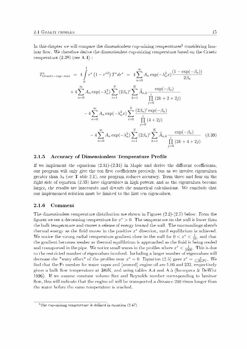
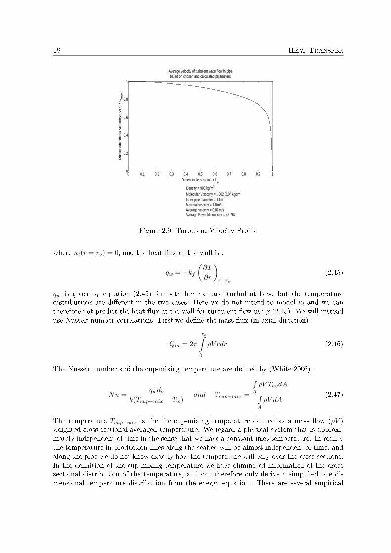
Area-averaging the mean velocity still give a good approximation to V(r) over the cross sectionexcept near the wall (see 2.9). The velocity pro�le displayed in Figure 2.9 is derived from ananalytical expression of the eddy di�usivity (Quarmby & Anand 1969). Based on this pro�lewe further introduce an area-averaged velocity :
V =2r2o
ro∫0
rV (r)dr (2.42)
It is now of interest to investigate the loss of energy to the surroundings as a consequenceof heat loss from the bulk �ow through the pipe wall. Since the �ow is turbulent, the timeaveraged thermal energy equation should be considered. When axial heat conduction anddissipation is neglected, the equation will be (see B.1-B.7) :
V∂T
∂x=
1r
∂
∂r
(r
∂
∂r(κ + κt)
∂T
∂r
)(2.43)
where κ and κt are the thermal di�usivities, molecular and turbulent, respectively. κt mustbe given to allow equation (2.43) to be solvable, for example as a correlation or by turbulencemodeling. It follows from (2.43) that the radial component of the heat �ux vector isgiven by :
qr = −ρCp (κ + κt)∂T
∂r(2.44)
18 Heat Transfer
0 0.1 0.2 0.3 0.4 0.5 0.6 0.7 0.8 0.9 10
0.2
0.4
0.6
0.8
1
Dimensionless radius: r / ro
Density = 998 kg/m3
Molecular Viscosity = 1.002 ⋅ 103 kg/sm Inner pipe diameter = 0.1m Maximal velocity = 1.0 m/s
Average velocity = 0.89 m/s Average Reynolds number = 46 767
Dim
ensio
nle
ss v
elo
city: V
(r)
/ U
max
Average velocity of turbulent water flow in pipebased on chosen and calculated parameters
Figure 2.9: Turbulent Velocity Pro�le
where κt(r = ro) = 0, and the heat �ux at the wall is :
qw = −kf
(∂T
∂r
)r=ro
(2.45)
qw is given by equation (2.45) for both laminar and turbulent �ow, but the temperaturedistributions are di�erent in the two cases. Here we do not intend to model κt and we cantherefore not predict the heat �ux at the wall for turbulent �ow using (2.45). We will insteaduse Nusselt number correlations. First we de�ne the mass �ux (in axial direction) :
Qm = 2π
ro∫0
ρV rdr (2.46)
The Nusselt number and the cup-mixing temperature are de�ned by (White 2006) :
Nu =qwdo
k(Tcup−mix − Tw)and Tcup−mix =
∫A
ρV TavdA∫A
ρV dA(2.47)
The temperature Tcup−mix is the the cup-mixing temperature de�ned as a mass �ow (ρV )weighted cross sectional averaged temperature. We regard a physical system that is approxi-mately independent of time in the sense that we have a constant inlet temperature. In realitythe temperature in production lines along the seabed will be almost independent of time, andalong the pipe we do not know exactly how the temperature will vary over the cross sections.In the de�nition of the cup-mixing temperature we have eliminated information of the crosssectional distribution of the temperature, and can therefore only derive a simpli�ed one di-mensional temperature distribution from the energy equation. There are several empirical

2.2 Heat Transfer in Pipe with Stationary Turbulent Flow 19
models for the Nusselt number in a smooth pipe with turbulent �ow, and in the literature(Incropera & DeWitt 1996) the most recommended is the Pethukov model :
Nu =(f
8 )RedoPr
1, 07 + 12, 7(f8 )
12 (Pr
23 − 1)
, Redo =V · do
ν, Pr =
Cp ·µkf
(2.48)
The Pethukov friction factor f is given by :
f = (0.790 ln Redo − 1.64)−2 (2.49)
and the Petukhov model is adapted for Reynolds and Prandtl numbers within the respectiveintervals :
3 · 103 < Redo < 5 · 106 0.5 < Pr < 2, 000 (2.50)
For rough pipes a model developed by A.F. Mills could be considered (Mills 1979). To progressfurther with the energy balance equation (2.43), we area-average the equation using the de�-nitions of the cup mixing temperature and the mass �ux (see B.8-B.9), �nding :
QmCp∂Tcup−mix
∂x= −2πroqw (2.51)
By substituting the de�ned Nusselt number (2.47) and the heat �ux (2.45) into (2.51) we �ndby integration :
Tcup−mix = Tw + (To − Tw) exp(−πkfNu
QmCpx
)(2.52)
where Tcup−mix(x < 0) = To has been used as the boundary condition. To simplify thetemperature equation we introduce the dimensionless parameters :
T ∗cup−mix =Tcup−mix − Tw
To − Twand x∗ =
x
2ro(2.53)
Combining (2.51), (2.52) and (2.53) we �nd the following dimensionless temperature distribu-tion :
T ∗cup−mix = exp(−2roπkfNu
QmCpx∗)
(2.54)

20 Heat Transfer
2.3 Heat Conduction Through Pipe Wall for Laminar and Tur-
bulent Flow
We assume the �ow for both laminar and turbulent conditions to be stationary and fullydeveloped.
2.3.1 Laminar Flow
Figure 2.10: In�uence of Pipe Wall Included
For laminar �ow we have the velocity pro�le :
u (r) =β
4µ
(r20 − r2) where β = constant = −∂p
∂x(2.55)
The mass �ux can be derived exactly since we know the velocity pro�le :
Qm =πβr4
oρ
8µ(2.56)
A balance equation for the heat transfer through the wall is given by (see Figure 2.10) :
Uw(Te − Tiw)2πro∆x− kw∂T
∂r2πr∆x = 0 (2.57)
where Uw is the heat transfer coe�cient of the wall. Integration of (2.57) yields :
Uwro
kw
r1∫ro
1rdr =
Te∫Tiw
dT
Te − Tiw(2.58)

2.3 Heat Conduction Through Pipe Wall for Laminar and Turbulent Flow 21
We then achieve the heat transfer coe�cient of the wall :
Uw =kw
ro ln(
r1ro
) (2.59)
The overall heat transfer coe�cient related to our system is (see (B.10-B.20)) :
1Utot
=1hf
+1
Uw(2.60)
where hf is the heat coe�cient of the �uid inside the pipe given by :
hf =kfNu
2ro(2.61)
The (mean) Nusselt number for forced convection of fully developed laminar �ow inside acircular duct with constant wall temperature is given by (Hausen 1959) :
Nu = 3.657 +0.19
(Re Pr 2ro
L
)0.8
1 + 0.117(Re Pr 2ro
L
)0.467 where Re < 2300 (2.62)
L is the pipe length, and we consider a system where L � 2ro. It is therefore a goodapproximation to use Nu = 3.657. We may now derive the overall heat transfer coe�cientfrom the equations (2.60), (2.61) and (2.62). This can be used in our next statement; a balanceequation for the loss of energy in the �ow direction and for the transfer of thermal energyfrom the �uid through the pipe wall. The dimensions involved are energy per unit time andper unit length :
QmCp∂Tcup−mix
∂x= 2πroUtot(Te − Tcup−mix) (2.63)
Integration with boundary conditions (see Figure 2.11) gives :
Tcup−mix = Te + (To − Te) exp(−16µUtot
βr3oρCp
x
)(2.64)
Let us simplify the temperature function by introducing the dimensionless variables :
T ∗cup−mix =Tcup−mix − Te
To − Teand x∗ =
x
2ro(2.65)
The dimensionless temperature for laminar �ow is then :
T ∗cup−mix = exp(−32µUtot
βr2oρCp
x
)(2.66)
2.3.2 Turbulent Flow
For turbulent �ow conditions we can now express the general dimensionless temperature dis-tribution along a pipe in a similar way as for the laminar. It is then important to use theoverall heat transfer coe�cient Utot related to turbulent �ow. There exist several empiricalmodels of the heat transfer coe�cient considering turbulent �ow. We have already introducedthe Pethukov Nusselt correlation from equations (2.48) and (2.49) and can therefore derive

22 Heat Transfer
the heat transfer coe�cient of the �uid from (2.61). The expression for Utot is established in(2.60), and it is straight forward to derive the overall heat transfer coe�cient for turbulent�ow conditions, as well. The temperature distribution is almost the same as (2.64) except forthe mass �ow and the overall heat transfer coe�cient. The temperature for turbulent �ow istherefore :
Tcup−mix = Te + (To − Te) exp(−2πroUtot
QmCpx
)(2.67)
or in dimensionless form :
T ∗cup−mix = exp(−4πr2
oUtot
QmCpx∗)
(2.68)
2.3.3 Deriving the Inner Wall Temperature
We �nd the inner wall temperature Tiw by assuming that the total heat exchange from the�uid to the environments must equal the transfer of thermal energy from the bulk�ow to thepipe wall. Our balance equation becomes :
Utot(Te − Tcup−mix) = hf (Tiw − Tcup−mix) (2.69)
After some manipulation we achieve a result that can be used for both turbulent and laminar�ow. We already know that the heat transfer coe�cient related to the �uid is di�erent forlaminar and turbulent �ow. The general inner wall temperature is :
Tiw = Tcup−mix −Utot
hf(Tcup−mix − Te) (2.70)

2.4 Influence of Pipe Wall Including an Uniform Insulation on the Inside 23
2.4 In�uence of Pipe Wall Including an Uniform Insulation on
the Inside
We assume that the insulation inside the pipe is of constant thickness everywhere on the innerwall. The overall heat transfer coe�cient Utot will then be expressed as below for the generalcase :
1Utot
=1hf
+1Ui
+1
Uw(2.71)
We have included an insulating wall layer through the heat transfer coe�cient Ui in theequation above. We derive Ui in the same way as we did for the heat transfer coe�cient of thewall -establishing a balance equation for the heat transfer through the insulation (see Figure2.11) :
Ui(Tw − Tiw)2πro∆x− ki∂T
∂r2πr∆x = 0 (2.72)
Figure 2.11: In�uence of Insulation and Pipe Wall
Integration of (2.72) gives the heat transfer coe�cient of the insulation :
Ui =ki
ro ln(
rori
) (2.73)
It is now possible to derive the overall heat transfer coe�cient for laminar and turbulent�ow by combining the already given heat transfer coe�cients of �uids and of insulation with

24 Heat Transfer
(2.71). The temperatures are already given by the equations, (2.64)-(2.65) or (2.67)-(2.68).Remember to replace ro with ri (see Figure 2.11) when using the mentioned equations.

2.5 Analysis of Wax Deposition 25
2.5 Analysis of Wax Deposition
We consider a simpli�ed situation where the condensate is being transported and cooledthrough a horisontal pipe with circular cross section. The �ow is considered stationary andturbulent. The condensate is further divided into three components, liquid (l), dissolved waxand wax crystals (d) and solid wax (w). The liquid is determined to be the lighter hydrocarboncomponents in the condensate. The dissolved wax is the same as dissolved para�ns and waxcrystals, where crystals are precipitated para�ns in the bulk �ow. The solid wax representthe deposit on the pipe wall. We consider a situation of only wax in the deposit; that liquidcomponents are not involved in the deposition process. We also consider wax deposition tooccur in a localized area in the pipe (see Figure 2.12) and that the wax deposit is a uniformand concentric layer of constant thickness. The balance equations for the problem is givenbelow.
Figure 2.12: Localized deposition

26 Heat Transfer
2.5.1 Balance Equations
Mass Conservation
We introduce a balance equation for the �uid component (d) that contains para�ns using thecontrol volume method (see Figure 2.12) :
d
dt
∫VG(t)
ρddV +∫
AG(t)
ρd(vd − vG) · dA = 0 (2.74)
Here ρd and vd are the density [ kgm3 ] and the velocity �eld [ms ] of the given phase related to the
mass exchange with deposit on wall. AG and VG are the geometrical area [m2] and volume[m3] considered (with the inner radius) of the inside pipe. vG is the velocity �eld related toany changes of VG or AG over time. We further assume time independent mass identities anduse space averages as needed to rewrite (2.74) :
π(x1 − xo)ρdd
dtr2i (t) + Qx(xo)−Qx(x1)−Qw(ri) = 0 (2.75)
where ρd is the volume average density of the hydro-carbon components involved. Qx and Qw
are the axial and radial mass �ow rates, respectively, evaluated at locations as indicated inFigure 2.12. By de�nition we have :
Qw(ri) = 2πri(x1 − xo)ρwdH
dt(2.76)
where we assume H to be dependent of the two parameters, time and inner wall temperature,to get :
dH
dt=
∂H(t, Tiw)∂t
+∂H(t, Tiw)
∂Tiw
∂Tiw
∂t(2.77)
By de�nition we also have :
Γw = ρwdH
dt(2.78)
Due to lack of information (measurements) about Qx, it is hard to simplify the mass balanceequations given above.
Momentum Conservation
We assume no gravitational contributions during deposition. We also assume the wax tooccupy the total surface on the inner pipe wall within the localized area.Thus the momentum equation is (Schulkes 2006) :
∂
∂t(ρlAlul)−
∂
∂x(ρlclu
2l Al) =
∂
∂x(PlAl) +
∂
∂x
(µe
l Al∂ul
∂x
)− Slτlw
Ai(2.79)
where Pl is the axial pressure ([Pa]) of the liquid, µel = µl + µT is the molecular and eddy
viscosity ([ kgsm ]), Sl is the liquid perimeter wetter ([m]), τlw is the wall shear stress ([ kg
s2m])
caused by the liquid, and cl is de�ned as cl = 1Alu
2l
∫Al
u2ndS. We hereby declare cl ≡ 1.

2.5 Analysis of Wax Deposition 27
Energy Conservation
We assume the bulk temperature to be independent of time during deposition. An assumptionthat is reasonable for a �nite temperature di�erence between the bulk �ow and the coolingenvironment, where changes of the bulk temperature is ignorable during the transportationfrom x = xo to x = x1. The energy equation of relevance is discussed in Sections 2.1-2.4. Wetherefore combine equations (2.51) and (2.47) of Section 2.2 to �nd :
∂Tcup−mix
∂x= −
πklNu(Tcup−mix − Tcooling)QlCp,l
(2.80)
where :
Nu = −2ri
(∂T∂r
)r=ri
Tcup−mix − Tcooling(2.81)
The rewritten inner wall temperature based on equation (2.70) of Section 2.3 is :
Tiw = Tcup−mix −Utot
hl(Tcup−mix − Tcooling) (2.82)
2.5.2 Considerations
As will be shown in Chapter 4, deposition is a delayed process. It can be shown that atypical mass di�usion time scale (tw) for deposition is much smaller than the time scale formass transportation in the axial direction. Since the liquid is assumed to not in�uence thedeposition, we further assume constant axial velocity of the oil. In addition we consider thedissolved wax to be transported with the same velocity as the liquid in the axial direction;thereby ul ≡ ud = const. A typical time scale for molecular transportation with bulk �ow inthe axial direction is ttransp ∼ x1−xo
ul. Based on typical axial velocities used in the deposition
experiments in Chapter 4, an estimated time scale for this transportation is ttransp ∼ 2s, whiletw is much larger.We therefore state tw � ttransp. We also assume the densities to be constant and independentof time and the wax thickness (H) to be small compared to the inner pipe radius (ro). Wetherefore assume the following relation between the wax thickness and inner steel pipe radius;Hro
= ε � 1.
Simpli�cations of Impulse Conservation
Assuming steady state conditions and fully developed �ow, the impulse equation can be written:
∂Pl
∂x= −Slτlw
Al(2.83)
2.5.3 Analysis of Γw
We analyse the mass transfer toward the wall, considering the time scale, t � 4r2o
ν . We alwaysassume the wax thickness (H) considered to be very small compared to the inner radius ofthe steel pipe (ro). To simplify the problem, we assume the inner wall temperature to beindependent of time, that ∂Tiw
∂t = 0. This is not unreasonable if the inner wall temperaturechange very little when a small layer of wax has been established on the wall. In Chapter 4, we
28 Heat Transfer
will �nd that the inner wall temperature increases fast in the initial period of each experimentand that it seems to stabilise close to the incoming oil temperature.
From these assumptions we obtain the following mass transfer rate :
Γw = ρw∂H
∂t(2.84)
Including results from Chapter 5 where we derive correlation curves on the form H ≈ Btα,gives :
Γw = Bαρwtα−1 (2.85)
The mass transfer rate, equation (2.88) above, is decreasing for increased t since α − 1 < 0.This is what we expect based on the results of the calculated wax thickness that we presentin Chapter 4. There we will �nd a clear tendency of a damped increase of the wax thicknessover time.
The mass transfer (Γw) considering a small time scale, t � 4r2o
ν , is perhaps more compli-cated. Here we can not ignore the in�uence of the inner wall temperature. In the previouschapter we found correlation curves where the inner wall temperature where not involved. Wedid not �nd better correlations by involving the Tiw. We believe that the inner wall tem-perature has an important impact on the deposition, especially in the beginning of the waxprocess.
Note, we may have a singularity at t = 0. To evaluate this, more details is needed.
2.5.4 Conclusion
In this section, we introduced the balance equations used to evaluate the wax problem con-sidering simpli�ed conditions. From the considerations, the impulse conservation, equation(2.86) is the same as the hydraulic balance equation that we introduce in Chapter 4 (Section4.2) where we establish the pressure drop method. In respect to mass balance and mass �uxtoward the wall, we derived the rate of deposition and information from Chapter 5 is included
to derive the rate of deposition for a larger time scale, where t � 4r2o
ν . When it comes toevaluating the initial rate of deposition, more details than we have here are needed.
Chapter 3
Temperature Distributions - A
Summary
The temperature equations that we found in section 2.2, 2.3 and 2.4 must be used with caution.Simpli�cations as area averaging and assumptions of constant �uid properties were applied.Both local (Graetz) and integral methods were used. It is of interest to compare the resultsobtained by the di�erent methods in a consistent way. We expect that with turbulent �ow in apipe, the transfer of thermal energy per square unit at the wall will be more e�ective comparedto laminar �ow. This is one of the main properties that di�erentiate turbulent from laminar�ow. When it comes to including an insulating layer or not, we expect that with insulationthe decrease in temperature as the �uid is transported will be less than without insulation.In�uence of the insulation clearly depends on both its thickness and its thermal conductivity.In section 2.3 we introduced the temperature distribution for stationary turbulent �ow usingthe Petukhov Nusselt correlation. In section 2.4 the temperature distribution based on heatconduction through the �uid and the pipe wall. In section 2.5, same as in section 2.4, but inaddition we included an insulating layer.
3.1 Temperature Distributions
In this chapter we always consider constant �uid properties. We base the results on unusedengine oil with the given properties at 320K (Incropera & DeWitt 1996). The inner pipe radiusis set to be ro = 50mm, the thickness of the pipe wall to be 8mm, and a uniform thicknessof the insulation to be 0.5mm. We further de�ne the heat conductivity of the insulation tobe two times that of oil, kins = 2koil, where koil = 0.143 J
smK . The heat conductivity ofpara�ns are about two times larger than the heat conductivity of the condensate (Incropera& DeWitt 1996). That means, we can draw a parallel between the results obtained from theengine oil and the insulated pipe in this chapter, with the condensate and a small wax layerthat are discussed in Chapter 4. The density of the engine oil is ρoil = 871.8 kg
m3 and the
kinematic viscosity is given to be νoil = 1.61 · 10−4m2
s Further we chose the �ow rates to be
Qlam = 5.0 · 10−3 m3
s for laminar �ow and Qturb = 5.0 · 10−1 m3
s for turbulent �ow. Main codesfor numerical calculations are given in the last Section of Appendix (Maple).

30 Temperature Distributions - A Summary
3.1.1 Laminar Flow
0.5 1 1.5 2 2.5 3x 10
5
0
0.1
0.2
0.3
0.4
0.5
0.6
0.7
0.8
0.9
1
x/d
o
T*
0.039
Figure 3.1: Dimensionless cup-mixing temperatures considering laminar �ow
◦ : temperature from the integral method, equation (2.63) where Uw = 0• : temperature from Graetz problem, equation (2.39)
Figure 3.1 indicates a small di�erence between the pro�le based on laminar �ow using theintegral method and the resulting pro�le from Graetz problem. Both represent dimensionlessmixing temperatures and are derived in two di�erent ways. For a few eigenvalues we cannot expect the mixing (Graetz) temperature to be representative for x∗ = 0 due to the slowmathematical convergence of the coe�cients given by (2.28). By comparing the equation(2.38) with di�erent numbers of eigenvalues (four or more), we �nd that, for the dimensionlessx∗ de�ned in equation (2.5), the di�erence in the pro�les where x∗ ≥ 1
100 is less than 1%. Forthe case, we keep in mind that the dimensionless x∗ de�ned for the solution of the Graetzproblem is not the same as the scale used in this chapter. It is therefore necessary to do atransformation to the dimensionless x
doused in Figures 3.1 - 3.3. The do is the inner pipe
diameter, and we can safely compare the dimensionless (Graetz) temperature pro�le withothers found from the integral method when x
do≥ 3900. The mixing temperature from the
integral solution is based on constant wall temperature to make it comparable with the mixing(Graetz) temperature. It is important to mention that the Graetz pro�le in the �gure aboveis valid only if EcPr ' 0.392
To−Te� 1 and Pe ' 7.7 ∗ 106 ·L � 1. L represents the length of
the pipe considered, and the Peclet relation is clearly true for a several meters pipe length.The Eckert-Prandtl relation holds true if the di�erence between the inlet and environmentaltemperature is hold within a restricted interval.

3.1 Temperature Distributions 31
Figure 3.2: Dimensionless temperature pro�les from the integral method
◦ : temperature distribution with (0.5mm) insulation on the inner pipe wall, equation (2.66)− : temperature distribution with no insulation on the pipe wall, equation (2.66)
There is no di�erence in the temperature pro�les in Figure 3.2, considering an insulatinglayer on the wall or not. We expect the insulation thickness to be larger or the heat conductiv-ity to be much lower to achieve a clear di�erence. An interesting aspect is how the insulationin�uences the temperature drop more clearly under turbulent �ow (see Figure 3.3) comparedto that of laminar �ow above. This is due to the strong property of heat transfer within theturbulent �ow. The turbulence will try to eliminate the heat while the insulation will resistmuch of the thermal energy from transferring through the pipe wall. We can say that, underturbulent �ow conditions, the insulation and its resistance to thermal conduction is workingharder compared to when it is exposed to laminar �ow, or simply, that the laminar �ow bettertransports the thermal energy in the axial direction with less loss to the environment.

32 Temperature Distributions - A Summary
3.1.2 Turbulent Flow
0.5 1 1.5 2 2.5 3 3.5 4 4.5 5x 10
5
0
0.1
0.2
0.3
0.4
0.5
0.6
0.7
0.8
0.9
1
x/do
T*
0
Figure 3.3: Dimensionless temperature pro�les from the integral method
∗ : temp. distrib. in�uenced by (0.5mm) insulation on the inner pipe wall, equation(2.68)• : temp. distrib. based on a clean pipe (no insulation), equation (2.68)
◦ : temp. distrib. based on a clean pipe with constant wall temperature, equation (2.54)
From Figure 3.3, we see that the in�uence of a thin layer of insulation inside the pipe resultin a much slower decreasing temperature as the �uid moves from a point to another in theaxial direction compared to the pro�les of a clean pipe. The temperature di�erence is smallconsidering the pro�le based on a clean pipe with constant inner wall temperature (◦) whereUw = 0, compared to the pro�le with a variable inner wall temperature (•) where Uw = Usteel.We keep in mind that the occurrence of a thin layer of wax, will, as can be seen in the �gure,cause the temperature in a tube under turbulent conditions to change in a pronounced way.

3.1 Temperature Distributions 33
Figure 3.4: Inner wall temperatures considering turbulent �ow
� : inner wall temperature derived with a 0.5mm insulation (see equation (2.70)).− : inner wall temperature derived with no insulation, (see equation (2.70))
The last �gure of this chapter, Figure 3.4, depicts the inner wall temperatures of turbulent�ow. The temperature distribution at the wall is of interest, especially when consideringturbulent �ow in an insulated pipe. As mentioned in the introduction, the precipitation ofwax in crude is dependent of the temperature di�erence between the inside/outside pipe wall.The process where wax deposits on a cold surface will provide an insulating layer on the wall(in physical contact with the �ow) causing the temperature to quickly change from lowerto higher. This is due to the much lower heat transfer coe�cient of wax compared to thepipe wall of steel. A prediction of the temperature along the inside wall is important to theunderstanding of the wax process. Figure 3.4 is based on unused engine oil at 320K, assumingan incoming constant temperature of 325K, and an outside wall temperature of 315K whenthe �ow pass a certain axial location in the pipe. The dimensions of the pipe, insulation, andthe �ow rate is exactly the same as described in the beginning of this chapter. We still assumethe constant properties of the oil given at 320K (Incropera & DeWitt 1996). Note that wehave calculated the inner wall temperature with or without an insulation of 0.5mm comparedto a much larger inner radius of the steel pipe (50mm). By the inlet of the incoming �uid wehave a temperature di�erence about 3.8 ◦C, which must be considered a signi�cant di�erencedespite the small insulation thickness.

34 Temperature Distributions - A Summary
3.2 Conclusion
Considering laminar �ow, the temperature derived from the integral method is very much thesame as the result derived from Graetz problem. We have discussed two separate ways of solv-ing the energy equation (2.2) and found that deriving a mathematical solution to the Graetzproblem is much more time-consuming. We have solved the Graetz problem by mathematicalanalysis and we have found that a simpli�ed model from the integral method seems to be ingood agreement with our result. From numerical analysis the average di�erence between thetwo graphs are 2.8% for the plotted interval in Figure 3.1. The di�erence seems to be largestfor the �rst part of the interval and the analysis give an average di�erence of 7.1% within3900m < x < 105m. We will on the basis of these results expect good agreement for turbu-lent �ow related to the Graetz problem. We explain this from the expectation of a (Graetz)temperature distribution for turbulent �ow that is similar to the one found for laminar �ow,with the exception of a larger damping of the temperature as a function of the mass �ow inaxial direction.
Finally, an important result of this chapter, is the signi�cant di�erence of the inner walltemperature with or without a small insulating layer on the inner pipe wall under turbulent�ow conditions. This is an interesting aspect of the study of how the inner wall tempera-ture change in the occurrence of a small wax layer, and how this change of temperature willin�uence the physics related to the further deposition process.

Chapter 4
Experiments
In this chapter wax deposition measurements from pipe �ow experiments carried out at Sta-toilHydro's Research Department in Porsgrunn are analyzed and discussed. The results ofthe analysis indicate that the deposited wax has a pronounced in�uence on the wall boundarylayer temperature of the �owing oil. Eight deposition experiments are performed with con-stant �ow rates and constant incoming temperatures of the �uids. Among these, only six arerepresentative; those with the highest �ow rates. The reasons will be discussed in the analysisbelow. We use the pressure drop method to calculate the thickness of wax deposits. Prior toeach wax experiment, we assume constant inner wall temperature and introduce temperaturevariations in the pipe wall. We will �nd that the inner wall temperature seems to changemuch in the beginning of each experiment. First, we choose to neglect the in�uence of theroughness of the wall. Finally, we discuss the in�uence of a small roughness.
Figure 4.1: Wax surfaceThis picture illustrates a smooth surface of the wax layer from the condensate used. The
picture is taken by StatoilHydro.

36 Experiments
We introduce a picture of the test rig in Figure 4.2 below. The picture show the facilityused to perform the experiments discussed in this chapter.
Figure 4.2: Picture of the facility
The line marked T.S. is the test section and the visible outer pipe is the water jacketenclosing the test pipe of oil. The test section is removable by disconnecting the �anges on
each side. The picture is taken by StatoilHydro.
4.1 Facility Description
A sketch of the pipe �ow facility used in the experiments is shown in Figure 4.3 where themain components of the facility are indicated. Two pumps generate the pressure levels neededto obtain the appropriate �ow rates of the test �uid and the coolant, respectively. The testpipe is a 5.55m long steel pipe with an inner diameter of 0.0526m, and a wall thickness corre-sponding to 0.0039 cm. The test pipe is enclosed by a cooling jacket with an inner diameterof 0.1397m. Fully developed turbulent �ow of the condensate is assumed. Temperatures ofboth the condensate and the coolant water were measured at the inlet and the outlet of thetest section. The pressure at both inlet and outlet of the test pipe was also measured and thepressure drop is used to calculate the wax thickness. The accuracy of the pressure measure-ments is therefore crucial for the reliability of the wax thickness calculations. The density hasalso been measured during the experiments performed.

4.1 Facility Description 37
4.1.1 Properties of Condensate Used in Wax Deposition Experiments
The density measured during wax deposition experiments are typically :ρoil = 824 kg
m3 at Toil = 15oC
ρoil = 819 kgm3 at Toil = 20oC
ρoil = 813 kgm3 at Toil = 30oC
ρoil = 806 kgm3 at Toil = 40oC
The molecular viscosity is derived from interpolation of the following (rheometer) data :Toil = [12.4658, 20.2073, 30.0067, 39.7039, 49.4686, 59.2560]oCµoil = 10−3 · [3.8, 2.8, 2.2, 1.8, 1.5, 1.3] kg
sm
The thermal conductivity: koil = 0.1344 JsmK
The heat capacity of the oil: Cpoil = 1950 JkgK

38 Experiments
Figure 4.3: Sketch of the facilityThe �gure shows a sketch of the pipe �ow facility used in the experiments. The main
components are indicated in the �gure.
Figure 4.4: Details of the test section
ri : inner pipe radius available for �ow of oilro : inner steel pipe (test pipe) radiusr1 : outer steel pipe/test pipe radiusr2 : inner pipe radius of water jacket
L : length of test section

4.2 Pressure Drop and Wax Thickness 39
4.2 Pressure Drop and Wax Thickness
A formula relating the wax thickness to the pressure drop will now be established. When waxdeposits on the pipe wall, the cross section will decrease and cause an increase in the pressuredrop for constant �ow rates. If we assume the condensate to be incompressible and ignore thegravitational and accelerational pressure gradients, we get the following result from hydraulicforce balance (see Figure 4.5) :
(P (x)− P (x + L))πr2i − 2πriLτwall = 0 (4.1)
Figure 4.5: Hydraulic stresses
Thus :dP
dxLπr2
i − 2πriLτwall (4.2)
where a connection between the shear stress and the Darcy friction factor is (Schulkes 2006) :
τwall =18ρoil
(Qoil
πr2i
)2
fD (4.3)
Thus :dP
dx= −
ρoilQ2oil
4π2r5i
fD (4.4)
We derive the wax thickness from the following equation by replacing Darcy friction factorwith the best �t friction factor derived for non-isothermal �ow :
dP
dx=
ρoilQ2oil
4π2r5i
fBF (4.5)
where :ri = ro −H (4.6)
H is the wax thickness and fBF is the best �t friction factor formula subject to the �owcondition in the experiments reported here. The procedures used to obtain the fBF -formulasare discussed in section 4.4.
40 Experiments
4.3 Inner Wall Temperature and Wax Thickness
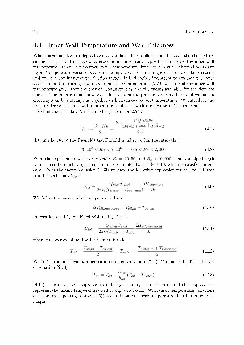
When para�ns start to deposit and a wax layer is established on the wall, the thermal re-sistance in the wall increases. A growing and insulating deposit will increase the inner walltemperature and cause a decrease in the temperature di�erence across the thermal boundarylayer. Temperature variations across the pipe give rise to changes of the molecular viscosityand will thereby in�uence the friction factor. It is therefore important to evaluate the innerwall temperature during a wax experiment. From equation (2.70) we derived the inner walltemperature given that the thermal conductivities and the radius available for the �ow areknown. The inner radius is always evaluated from the pressure drop method, and we have aclosed system by putting this together with the measured oil temperatures. We introduce thetools to derive the inner wall temperature and start with the heat transfer coe�cientbased on the Pethukov Nusselt model (see section 2.2) :
hoil =koilNu
2ri=
koil(
fBF8
)RePr
1,07+12,7(fBF
8)12 (Pr
23−1)
2ri(4.7)
that is adapted to the Reynolds and Prandtl number within the intervals :
3 · 103 < Re < 5 · 106 0.5 < Pr < 2, 000 (4.8)
From the experiments we have typically Pr = [20, 50] and Re > 10, 000. The test pipe lengthL must also be much larger than its inner diameter D, i.e. L
D ≥ 10, which is satis�ed in ourcase. From the energy equation (2.63) we have the following expression for the overall heattransfer coe�cient Utot :
Utot =Qm,oilCp,oil
2πri(Twater − Tcup−mix)∂Tcup−mix
∂x(4.9)
We de�ne the measured oil temperature drop :
∆Toil,measured = Toil,in − Toil,out (4.10)
Integration of (4.9) combined with (4.10) gives :
Utot =Qm,oilCp,oil
2πri(Twater − Toil)∆Toil,measured
L(4.11)
where the average oil and water temperature is :
Toil =Toil,in + Toil,out
2, Twater =
Twater,in + Twater,out
2(4.12)
We derive the inner wall temperature based on equation (4.7), (4.11) and (4.12) from the useof equation (2.70) :
Tiw = Toil −Utot
hoil(Toil − Twater) (4.13)
(4.11) is an acceptable approach to (4.9) by assuming that the measured oil temperaturesrepresent the mixing temperatures well at a given location. With small temperature variationsover the test pipe length (about 1%), we anticipate a linear temperature distribution over itslength.

4.4 Friction Factor Formulas 41
4.4 Friction Factor Formulas
Before we start analysing the wax data, we estimate the precision of the pressure measure-ments. The inner diameter of the pipe is given as Do = 0.0525 ± 0.0003m. It is di�cult tomeasure the inner diameter and it is even more challenging to measure the roughness in apipe. It is often a good approximation to ignore roughness considering a technical smoothpipe, but in this study we assume it to be within the interval 0 ≤ ε ≤ 5 · 10−5m. We alsoassume a pressure o�set among the measuring data, and that the real pressure drop can beexpressed as ∆P = ∆Pmeasured ± poffset. For turbulent �ow conditions we choose Haaland'sformula to model the friction factor. Before the analysis of the wax deposition, we introduce acorrected friction factor. The Haaland factor is based on constant temperatures; an isothermalsystem. If the environmental temperature deviates from the bulk �ow temperature and causeheat exchange within the system; we have a non-isothermal system.
4.4.1 Isothermal Experiments : No Deposition
We consider experimental data obtained in a clean and smooth pipe with variable �ow rates(of oil) to test the agreement between the Haaland (4.14) and the Darcy (4.15) friction factors.We have the same inlet temperature of water and oil; thereby an isothermal system. All the�ow rates considered involve turbulent �ow conditions.The Haaland friction factor is :
fH =
(1.8 log
(6.9
Reoil+(
εsteel
3.7Do
)1.11))−2
(4.14)
and the Darcy friction factor from hydraulic force balance is :
fD = − 4π2r5i
ρoilQ2oil
dp
dx(4.15)
We de�ne the measured pressure drop :
∆Pmeasured = Pin − Pout (4.16)
The calculated pressure based on the Haaland friction factor is :
∆Pcalculated =ρoilQ
2oilL
4π2r5i
fH (4.17)
We de�ne the error in the calculated pressure drop via :
erelative =∆Pmeasured −∆Pcalculated
∆Pmeasured(4.18)
Finally, the average of the absolute values of erelative :
Erelative =1N
N∑i=1
|erelative | (4.19)
Integration of (4.15) combined with (4.16) gives the equation we use to calculate the Darcyfriction factor. We always assume fully developed and turbulent �ow conditions, and we

42 Experiments
compare the Darcy with the Haaland friction factor through the equation (4.18). The Haalandfactor depends on both roughness and inner diameter of the pipe. Based on Tables C.1 andC.2 (in Appendix) we calculate the optimal roughness, inner diameter, and pressure o�set byvarying their values within restricted intervals (in a three dimensional parameter space) usingnonlinear optimalization to minimize Erelative. The best �t is given when εsteel = 0m andDo = 0.0526m, where we ignore the pressure o�set by setting poffset = 0 Pa. In Figure 4.6the error in the calculated pressure drop is less than 4.5% for all isothermal data. We therebyhave good agreement between the measured Darcy and the Haaland friction factors for thegiven diameter and roughness.
0 1 2 3 4 5 6 7 8 9x 10
−3
−0.03
−0.02
−0.01
0
0.01
0.02
0.03
0.04
0.05
Volume flow of oil [m3/s]
e rela
tive
Figure 4.6: Error in the calculated pressure drop for isothermal �ow, Tables C.1 and C.2 (seeAppendix)
4.4.2 Non-Isothermal Experiments : No Deposition
Radial temperature variations will occur when the �owing �uid is being cooled by heat lossesthrough the pipe wall. The molecular viscosity will thereby vary across the �ow, and thesevariations must be taken into account when the best friction factor model is evaluated. Inour evaluation of the experiments, we use the molecular viscosity measured in a rheometer(StatoilHydro 2007) with a reasonable accuracy (±4%). In general the molecular viscosity de-creases rapidly with temperature (White 2006). We will therefore expect a higher oil viscosityat the inner wall compared to that of the bulk �ow and this again increases the friction of thewall. For non-isothermal �ow a correction factor has been introduced(Perry & Chilton 1973) :
f = fBF = fH ·αcorrection (4.20)
where :
αcorrection =(
µwall
µbulk
)n
(4.21)

4.4 Friction Factor Formulas 43
and n = 0.11 or n = 0.17 in the case of cooling or heating. This correlation was developed(Sieder & Tite 1936) based on three di�erent oils. The intention was to study the e�ectof a radial temperature gradient on the distribution of the axial and radial components ofvelocity. Sieder and Tite proclaimed that this was not taken into consideration by (Graetz1885) or (Lévêque 1928). We consider a situation where the oil is being cooled and use thegiven exponent. We have derived the error in the calculated pressure drop using both theHaaland and the corrected friction factor (see Figure 4.7) on basis of non-isothermal data inTable C.3 (see Appendix). Figure 4.7 indicate a smaller error in the calculated pressure dropwhen using the corrected friction factor, but not su�cient small. We require that the errorin the calculated pressure drops are less than 0.05 (or 5%) for the case. In Figure 4.7 weexpect an optimal error in the calculated pressure drop for n in the interval 0 to 0.11, andfrom numerical calculations using all the non-isothermal data, we �nd the minimum Erelative
when n = 0.05(see Figure 4.8).
4.4.3 Discussion of the Isothermal and Non-Isothermal Data
The accuracy of the measuring instruments are very important, especially for the lowest �owrates and pressure drops. From the graphs in Figures 4.6 and 4.7 it is clear that the ∆Pmeasured
are larger than the ∆Pcalculated for the lowest �ow rates and opposite for several of the highestrates. It also appears to be a linear connection between the error in the calculated pressuredrop and the �ow rate in both Figures, and it is important to note the fact that any suchrelation should not occur. We therefore carry out a linear regression analysis based on thesetwo parameters for both isothermal and non-isothermal data. From the results we can notreject the hypothesis of a linear relation. In addition, the results based on isothermal dataseem to have a signi�cant auto correlation, which means that we might have a connectionbetween the measurements performed within each experiment. We carefully conclude that weobserve larger uncertainties among the lowest �ow rates, and a systematic relation can not beexcluded.

44 Experiments
1 2 3 4 5 6 7x 10
−3
−0.05
0
0.05
0.1
0.15
0.2
Volume flow of oil: [m3/s]
Circles : f = fH
⋅ αcorrection
, n = 0 Stars : f = f
H ⋅ α
correction , n = 0.11
Squares : f = fH
⋅ αcorrection
, n = 0.05
ere
lative
Figure 4.7: Error in calculated pressure drop for non-isothermal �ow, Table C.3 (see Appendix)◦ : Pressure drop using the Haaland friction factor
? : Pressure drop based on non-isothermal Sieder & Tite friction factor� : Pressure drop using the best �t (non-isothermal) friction factor.
0 0.01 0.02 0.03 0.04 0.05 0.06 0.07 0.08 0.09 0.10.46
0.48
0.5
0.52
0.54
0.56
0.58
0.6
0.62
0.64
n
|∆Erelative
|
Figure 4.8: Minimum value of |∆Erelative|By considering a precision of only two decimals, we �nd the minimum value of |∆Erelative|
for n = 0.05. The optimal pressure drop is based on non-isothermal data.

4.5 Experimental Results 45
4.5 Experimental Results
We have eight wax experiments performed by StatoilHydro available to study. Unfortunately,we can not include all in further work using the adapted friction factor. The initial large errorin the calculated pressure drop among two of the wax experiments with �ow rates equal to 5m3/h and 10 m3/h can not be ignored. In Figure C.1 (see Appendix) we have marked the twoexperiments showing a erelative of 0.172 and 0.132. The adapted friction factor is therefore aninaccurate approximation to these. In the continuation we will focus on the other six where theerelative is less than 0.4 (see Figure C.1 in Appendix). Let us �rst introduce the six experimentsinvolved. The experiments are named through the general matrix Toil,in − Twater,in − Qoil,where Toil,in and Twater,in are the measured incoming oil and water temperatures in ◦C and
Qoil is the volume �ux in m3
s .
4.5.1 Observed Pressure Drop With Comments
The measured pressure drops ∆Pmeasured (4.16) are presented in Figures 4.9 - 4.11. The pres-sure drops in all experiments increase with elapsed time, indicating that a growing wax layeris formed on the inside of the test pipe. We notice the most rapid growth of the pressure dropearly in the experiments. The reduced growth rate with time is attributed to the temperaturedevelopment in the wall boundary layers of the �owing test �uid. A wax layer on the insideof the test pipe increases the thermal resistance across the pipe wall and causes an increase inthe boundary layer temperature as discussed in section 4.5.2.The observed pressure drops are �uctuating for some reason. The typical �uctuation levelmay be estimated as an average deviation from a linear growth curve in a representativetime interval. In general, we have a series of N measurements in each experiment with thegiven time interval to, t1, .., tn, .., tN . Evaluation of a typical �uctuation level is based on themeasured pressure drops within the �xed time interval t ∈ [tm, tM ], where m = 0.65 ·N andM = 0.85 ·N . In Figure C.2 (see Appendix) ∆Pmeasured are considered linear in time, andfrom regression analysis we derive the linear graph D to each interval. We evaluate the typical�uctuation level of ∆Pmeasured by assuming D to represent the "�uctuation-free" pressuredrop for fully developed turbulent and stationary �ow conditions. The �uctuation level isdetermined from the following expression :
Fpressure = 100%1
M −m
M∑q=m
∣∣∣∣∆Pmeasured,q −Dq
∆Pmeasured,q
∣∣∣∣ (4.22)
The results are shown in Table 4.1 below.
Table 4.1: Fluctuation level of the measured pressure dropExperiment Toil,in − Twater,in −Qoil A typical �uctuation level in percent Standard deviation (Pa)
15− 10− 21 ∆Pmeasured ± 0.06% 6.4120− 10− 15 ∆Pmeasured ± 0.05% 2.7520− 10− 21 ∆Pmeasured ± 0.14% 13.2220− 10− 25 ∆Pmeasured ± 0.05% 6.9830− 10− 21 ∆Pmeasured ± 0.11% 10.0240− 10− 21 ∆Pmeasured ± 0.32% 28.85
46 Experiments
In table 4.1 the �uctuation level of the measured pressure drops seem to be small in allexperiments. It should be mentioned that the pressure drops related to the experiment 40−10− 21 indicate a statistical weak linearity compared to the other experiments for the giveninterval. We conclude that the pressure transducers seem to give su�cient accuracy duringthe experiments.
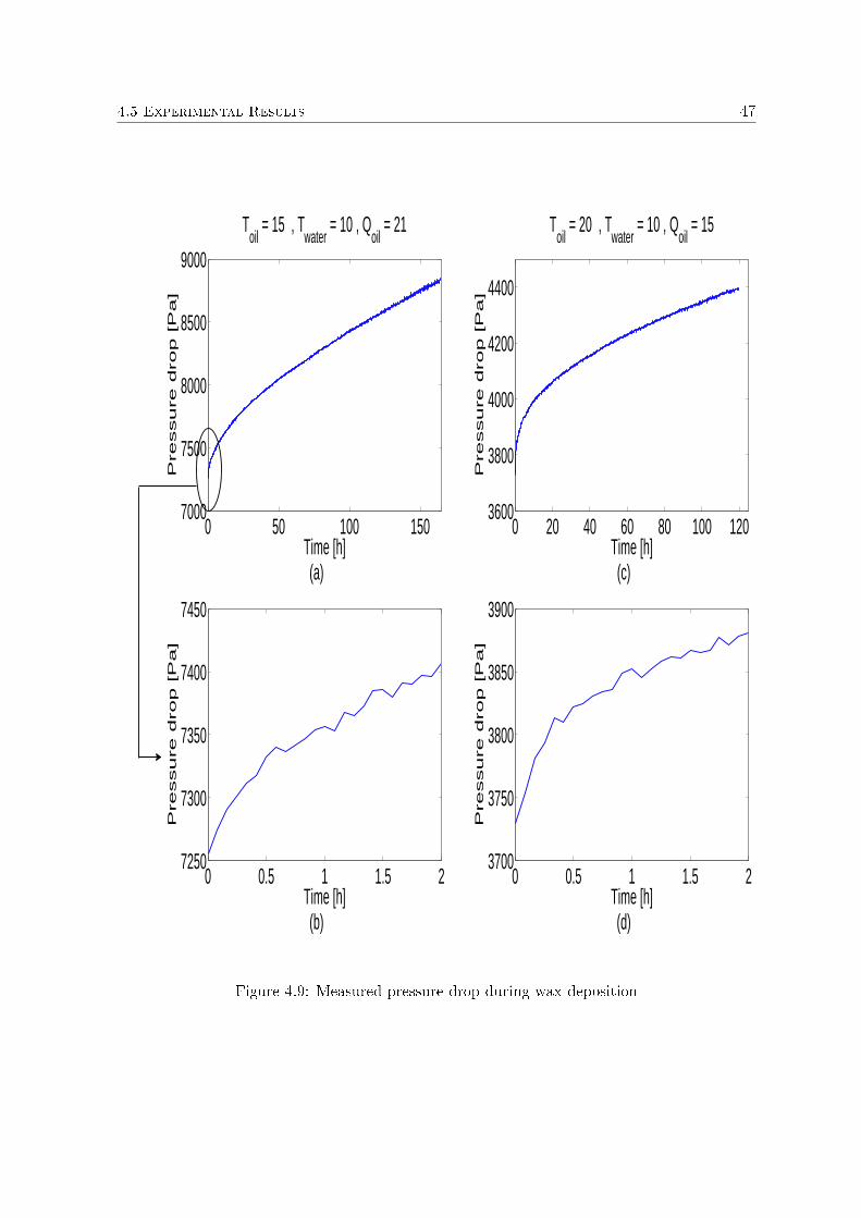
4.5 Experimental Results 47
0 0.5 1 1.5 27250
7300
7350
7400
7450
Time [h](b)
Pressure d
rop [P
a]
0 50 100 1507000
7500
8000
8500
9000
Time [h](a)
Pressure d
rop [P
a]
Toil
= 15 , Twater
= 10 , Qoil
= 21
0 20 40 60 80 100 1203600
3800
4000
4200
4400
Time [h](c)
Pressure d
rop [P
a]
Toil
= 20 , Twater
= 10 , Qoil
= 15
0 0.5 1 1.5 23700
3750
3800
3850
3900
Time [h](d)
Pressure d
rop [P
a]
Figure 4.9: Measured pressure drop during wax deposition

48 Experiments
0 20 40 60 80 1006500
7000
7500
Time [h](a)
Pressure d
rop [P
a]
Toil
= 20 , Twater
= 10 , Qoil
= 21
0 0.5 1 1.5 26500
6600
6700
6800
6900
Time [h](b)
Pressure d
rop [P
a]
0 10 20 30 40 50 609000
9500
10000
10500
Time [h](c)
Pressure d
rop [P
a]
Toil
= 20 , Twater
= 10 , Qoil
= 25
0 0.5 1 1.5 29300
9400
9500
9600
Time [h](d)
Pressure d
rop [P
a]
Figure 4.10: Measured pressure drop during wax deposition

4.5 Experimental Results 49
0 50 100 150 200 2506400
6600
6800
7000
7200
7400
Time [h](a)
Pressure d
rop [P
a]
Toil
= 30 , Twater
= 10 , Qoil
= 21
0 0.5 1 1.5 26440
6460
6480
6500
6520
6540
Time [h](b)
Pressure d
rop [P
a]
0 50 100 150 200 250 300 3506200
6400
6600
6800
7000
Time [h](c)
Pressure d
rop [P
a]
Toil
= 40 , Twater
= 10 , Qoil
= 21
0 0.5 1 1.5 26220
6240
6260
6280
6300
Time [h](d)
Pressure d
rop [P
a]
Figure 4.11: Measured pressure drop during wax deposition
Note that in experiment 40-10-21 the ∆Pmeasured seems to stabilise after 100h while inexperiment 30− 10− 21 the ∆Pmeasured continues to increase.

50 Experiments
4.5.2 Observed Temperature Drop and Derived Inner Wall Temperature
The measured oil temperature drops ∆Toil,measured (4.10) are presented In Figures 4.12 and4.13. A fast decrease of the temperature drop in the beginning of each experiment indicatethat thermal energy are prevented from transferring through the pipe wall as soon as para�nsdeposit on the wall. This phenomenon is a very important observation in our study and insection 3.2 we found that a small insulating layer will in�uence the inner wall temperaturesigni�cantly. This is exactly what we �nd by introducing the inner wall temperature given insection 4.3, and the results are presented in Figures 4.14 and 4.15. It is clear that the innerwall temperature changes quickly in the beginning of each wax experiment, and there is nodoubt that during the �rst hour or even the �rst minutes, it changes much compared to theinner wall temperature before deposition occurs. Large temperature di�erences between inletoil and water seem to give larger and faster changes of the inner wall temperature duringthe �rst minutes (see Figure 4.15 (c) and (e)). The temperature graphs based on experiment20 − 10 − 15 (see Figure 4.12 (c) and 4.14 (c)) indicate an increase of the temperature dropand a decrease of the inner wall temperature during the �rst minutes. This is not expectedto occur during wax deposition, and we consider it to be an initial condition of inaccuraciesin the measured oil temperatures. We further use the same procedure as in subsection 4.5.1to estimate a typical �uctuation level of the temperature transducers. We rede�ne the timeintervals with m = 0.45 ·N and M = 0.65 ·N . There are temperature �uctuations in everyexperiment, and we assume the temperature distribution to be approximately linear withinthe given intervals (see C.3) for the case of no �uctuations. It should be mentioned that thisis only an approximation we do to estimate the typical �uctuation level :
Ftemperature = 100%1
M −m
M∑q=m
∣∣∣∣∆Tmeasured,q −Dq
∆Pmeasured,q
∣∣∣∣ (4.23)
The results are shown in the table 4.2 under.
Table 4.2: Fluctuation level of the measured temperature dropExperiment Toil,in − Twater,in −Qoil A typical �uctuation level in percent Standard deviation (oC)
15− 10− 21 ∆Tmeasured ± 4.19% 0.003520− 10− 15 ∆Tmeasured ± 1.05% 0.003220− 10− 21 ∆Tmeasured ± 1.22% 0.003220− 10− 25 ∆Tmeasured ± 1.13% 0.002530− 10− 21 ∆Tmeasured ± 0.61% 0.004040− 10− 21 ∆Tmeasured ± 0.25% 0.0050
The typical �uctuation of the temperature measurements in the 20 − 10 − 15 experimentis about 1.05%. An adjustment of the initial measured incoming oil temperature with lessthan 0.7% is needed to give an increase of the inner wall temperature and a decrease of thetemperature drop during the �rst period. The inaccuracy can therefore explain the unexpectedinitial temperature drop and inner wall temperature related to this particular experiment. Ingeneral we have small �uctuations in the oil temperature measurements.

4.5 Experimental Results 51
0 1 2 3 4 5
0.2
0.25
0.3
0.35
Time [h](a)
Temperature difference of inlet/outlet oil during the first five hours.
Toil,m
easured [oC
]
0 20 40 60 80 100 120 140 1600
0.1
0.2
0.3
0.4
Time [h](b)
Toil,m
easured [oC
]
Temperature difference of inlet/outlet oil during the experiment.
0 1 2 3 4 5
0.4
0.5
0.6
0.7
Time [h](c)
Toil,m
easured [oC
]
0 20 40 60 80 100 1200
0.2
0.4
0.6
0.8
Time [h](d)
Toil,m
easured [oC
]
0 1 2 3 4 50.2
0.3
0.4
0.5
0.6
0.7
Time [h](e)
Toil,m
easured [oC
]
0 20 40 60 80 1000.1
0.2
0.3
0.4
0.5
0.6
Time [h](f)
Toil,m
easured [oC
]
Toil
= 15 , Twater
= 10 , Qoil
= 21
Toil
= 20 , Twater
= 10 , Qoil
= 15
Toil
= 20 , Twater
= 10 , Qoil
= 21
Toil
= 15 , Twater
= 10 , Qoil
= 21
Toil
= 20 , Twater
= 10 , Qoil
= 15
Toil
= 20 , Twater
= 10 , Qoil
= 21
Figure 4.12: Measured temperature drop during wax depositionNote that in �gure (c) the temperature drop is �rst increasing.

52 Experiments
0 1 2 3 4 50.25
0.3
0.35
0.4
0.45
0.5
Time [h](a)
Toil.m
easure
d [oC
]
Temperature difference of inlet/outlet oil during the first five hours.
Toil
= 20 , Twater
= 10 , Qoil
= 25
0 10 20 30 40 50 60 700.1
0.2
0.3
0.4
0.5
Time [h](b)
Temperature difference of inlet/outlet oil during the experiment.
Toil.m
easure
d [oC
] Toil
= 20 , Twater
= 10 , Qoil
= 25
0 1 2 3 4 5
0.8
1
1.2
1.4
Time [h](c)
Toil.m
easured [oC
] Toil
= 30 , Twater
= 10 , Qoil
= 21
0 50 100 150 200 2500.4
0.6
0.8
1
1.2
1.4
Time [h](d)
Toil.m
easured [oC
] Toil
= 30 , Twater
= 10 , Qoil
= 21
0 1 2 3 4 51.8
1.85
1.9
1.95
2
Time [h](e)
Toil.m
easured [oC
] Toil
= 20,Twater
= 10,Qoil
= 21
0 50 100 150 200 250 300 3501.6
1.7
1.8
1.9
2
Time [h](f)
Toil.m
easured [oC
] Toil
= 20,Twater
= 10,Qoil
= 21
Figure 4.13: Measured temperature drop during wax deposition

4.5 Experimental Results 53
0 1 2 3 4 510
12
14
16
18
Time [h] (e)
Tiw
[oC
]
Toil
= 20 , Twater
= 10 , Qoil
= 21
0 1 2 3 4 514
15
16
17
18
Time [h] (c)
Tiw
[oC
]
Toil
= 20 , Twater
= 10 , Qoil
= 15
0 1 2 3 4 510
11
12
13
14
Time [h] (a)
Tiw
[oC
]Derived inner wall temperature during the first five hours.
Toil
= 15 , Twater
= 10 , Qoil
= 21
0 20 40 60 80 100 120 140 16010
11
12
13
14
15
Time [h] (b)
Tiw
[oC
]
Derived inner wall temperature during the experiment.
Toil
= 15 , Twater
= 10 , Qoil
= 21
0 20 40 60 80 100 12014
15
16
17
18
19
Time [h] (d)
Tiw
[oC
]
Toil
= 20 , Twater
= 10 , Qoil
= 15
0 20 40 60 80 10010
12
14
16
18
20
Time [h] (f)
Tiw
[oC
]
Toil
= 20 , Twater
= 10 , Qoil
= 21
Figure 4.14: Inner wall temperatureInner wall temperature derived from the measured pressure drop and temperature drop in
the test pipe.Note that in �gure (c) the inner wall temperature is �rst decreasing.

54 Experiments
0 1 2 3 4 512
14
16
18
Time [h] (a)
Tiw
[oC
]Derived inner wall temperature during the first five hours.
Toil
= 20 , Twater
= 10 , Qoil
= 25
0 1 2 3 4 510
15
20
25
Time [h] (c)
Tiw
[oC
]
Toil
= 30 , Twater
= 10 , Qoil
= 21
0 1 2 3 4 516
18
20
22
24
26
Time [h] (e)
Tiw
[oC
]
Toil
= 40 , Twater
= 10 , Qoil
= 21
0 10 20 30 40 50 60 7012
14
16
18
20
Time [h] (b)
Tiw
[oC
]
Derived inner wall temperature during the experiment.
Toil
= 20 , Twater
= 10 , Qoil
= 25
0 50 100 150 200 25010
15
20
25
30
Time [h] (d)
Tiw
[oC
]
Toil
= 30 , Twater
= 10 , Qoil
= 21
0 50 100 150 200 250 300 35015
20
25
30
Time [h] (f)
Tiw
[oC
]
Toil
= 40 , Twater
= 10 , Qoil
= 21
Figure 4.15: Inner wall temperatureInner wall temperature derived from the measured pressure drop and temperature drop in
the test pipe.

4.5 Experimental Results 55
4.5.3 Wax Thickness Calculations
The wax thickness H is derived from integration of (4.5) combined with (4.16), (4.20)-(4.21),(4.7) and (4.9)-(4.13) :
H = ro −
(ρoilQ
2oilL
4π2∆PmeasuredfH
(µoil(Tiw)
µoil(Tcup−mix)
)0.05) 1
5
(4.24)
The wax thickness are calculated in two ways. One, assuming the initial inner wall temperatureof the test pipe to equal the average water temperature in the cooling jacket (Tiw(to) = Twater),or two, computing the initial inner wall temperature from (4.13). In both cases we assume noinitial wax on the pipe wall. The �rst (way) is reasonable since the thermal conductivity ofsteel is much higher than that of oil. The results are presented in Figures 4.16 and 4.17 ((a),(c) and (e)), where we note an initial negative wax thickness among four of the graphs. Next,we calculate the initial inner wall temperature to study its e�ect on the initial wax thicknesscalculation. The results are introduced in Figures 4.16 and 4.17 ((b), (d) and (f)), where wenote an improvement of the results, reducing the number of negative wax thicknesses fromfour to two. All the graphs show a positive wax thickness with the exception of experiments20 − 10 − 15 and 30 − 10 − 21. This is considered as an important observation of the factthat the inner wall temperature is of importance when deriving the wax thickness, especiallyin the beginning of a deposition process. It is also of interest to relate the negative waxthickness to the error in the measurements. We have already found a typical �uctuation levelamong the pressure and temperature transducers, indicating a minimum error related to themeasurements. In the wax thickness calculations, the �uctuations related to the pressuredrops will be further diminished by the small exponent 1
5 as indicated in the wax thicknessequation above. The negative wax thickness can therefore not be explained from a minimumerror corresponding to a typical �uctuation level in the wax calculations. We expect the errorto be larger than a typical �uctuation level, but the accuracy among the measurements is noteasy to determine from the information we have. In Figures 4.18 and 4.19 calculations basedon wax experiments during the whole time interval are presented. Finally, all the results areshown in Figure 4.20. We note among experiments 20− 10−Qoil (where Qoil = 15, 21, 25) in4.20, that a higher �ow rate gives a lower deposition thickness over time. This could connectthe results achieved to the Reynolds number and will be discussed in the coming chapter. Wealso note that a higher incoming oil temperature gives a smaller wax thickness over time. Thisis an interesting observation that can be connected to the quickly isolating e�ect of the waxlayer during the experiments. This will also be considered in the coming chapter.

56 Experiments
0 0.5 1 1.5 20
0.05
0.1
0.15
0.2
Time [h] (a)
Wa
x th
ickn
ess [m
m]
Calculated wax thickness based on initial inner wall temperature equal to average water temperature.
0 0.5 1 1.5 20
0.05
0.1
0.15
0.2
Time [h] (b)
Wa
x th
ickn
ess [m
m]
Calculated wax thickness where the initial inner wall temperature is derived from temperature variations in the pipe wall.
0 0.5 1 1.5 2−0.2
−0.1
0
0.1
0.2
Time [h] (c)
Wa
x th
ickn
ess [m
m]
0 0.5 1 1.5 2−0.2
−0.1
0
0.1
0.2
Time [h] (d)
Wa
x th
ickn
ess [m
m]
0 0.5 1 1.5 2
−0.2
−0.1
0
0.1
0.2
Time [h] (e)
Wa
x th
ickn
ess [m
m]
0 0.5 1 1.5 20
0.05
0.1
0.15
0.2
Time [h] (f)
Wa
x th
ickn
ess [m
m]
Toil
= 15 , Twater
= 10 , Qoil
= 21
Toil
= 20 , Twater
= 10 , Qoil
= 15
Toil
= 20 , Twater
= 10 , Qoil
= 21
Toil
= 15 , Twater
= 10 , Qoil
= 21
Toil
= 20 , Twater
= 10 , Qoil
= 21
Toil
= 20 , Twater
= 10 , Qoil
= 15
Figure 4.16: Calculated thickness of wax deposit
The di�erence in the initial wax thickness is shown. Note that experiment (d) give anegative wax thickness during the �rst minutes even though the estimated inner wall
temperature was included. The vertical scales in the Figures (e) and (f) are not equal, butwe con�rm that the graphs are just the same except for the initial wax thickness values.

4.5 Experimental Results 57
0 0.5 1 1.5 2−0.1
0
0.1
0.2
Time [h](f)
Wa
c th
ickn
ess [m
m]
0 0.5 1 1.5 2−0.1
0
0.1
0.2
Time [h](d)
Wa
x th
ickn
ess [m
m]
0 0.5 1 1.5 20
0.05
0.1
0.15
0.2
Time [h](b)
Wa
x th
ickn
ess [m
m]
Calculated wax thickness where the initial inner wall temperature is derived from temperature variations in the pipe wall.
0 0.5 1 1.5 20
0.05
0.1
0.15
0.2
Time [h](a)
Wa
x th
ickn
ess [m
m]
Calculated wax thickness based on initial inner wall temperature equal to average water temperature.
0 0.5 1 1.5 2−0.1
0
0.1
0.2
Time [h](c)
Wa
x th
ickn
ess [m
m]
0 0.5 1 1.5 2−0.1
0
0.1
0.2
Time [h](e)
Wa
c th
ickn
ess [m
m]
Toil
= 20 , Twater
= 10 , Qoil
= 25
Toil
= 30 , Twater
= 10 , Qoil
= 21
Toil
= 40 , Twater
= 10 , Qoil
= 21
Toil
= 20 , Twater
= 10 , Qoil
= 25
Toil
= 40 , Twater
= 10 , Qoil
= 21
Toil
= 30 , Twater
= 10 , Qoil
= 21
Figure 4.17: Calculated thickness of wax deposit
The di�erence in the initial wax thickness is shown. Note that experiment (d) give anegative wax thickness during the �rst minutes even though the estimated inner wall
temperature was included.

58 Experiments
0 20 40 60 80 100 120 140 1600
0.2
0.4
0.6
0.8
1
Time [h]
Wa
x th
ickn
ess [m
m]
Wax thickness.
0 20 40 60 80 100 120
0
0.5
1
Time [h]
Wa
x th
ickn
ess [m
m]
0 10 20 30 40 50 60 70 80 90 1000
0.2
0.4
0.6
0.8
1
Time [h]
Wa
x th
ickn
ess [m
m]
Toil
= 15 , Twater
= 10 , Qoil
= 21
Toil
= 20 , Twater
= 10 , Qoil
= 15
Toil
= 20 , Twater
= 10 , Qoil
= 21
Figure 4.18: Calculated thickness of wax deposit

4.5 Experimental Results 59
0 10 20 30 40 50 60 700
0.2
0.4
0.6
0.8
Time [h]
Wa
x th
ickn
ess [m
m]
Wax thickness.
0 50 100 150 200 250−0.2
0
0.2
0.4
0.6
0.8
Time [h]
Wa
x th
ickn
ess [m
m]
0 50 100 150 200 250 300 3500
0.2
0.4
0.6
0.8
Time [h]
Wa
x th
ickn
ess [m
m]
Toil
= 40 , Twater
= 10 , Qoil
= 21
Toil
= 30 , Twater
= 10 , Qoil
= 21
Toil
= 20 , Twater
= 10 , Qoil
= 25
Figure 4.19: Calculated thickness of wax deposit

60 Experiments
0 10 20 30 40 50 60 70−0.1
0
0.1
0.2
0.3
0.4
0.5
0.6
0.7
0.8
Time [h]
H [m
m]
Wax thickness calculations for all experiments.
15−10−2120−10−1520−10−2120−10−2530−10−2140−10−21
Figure 4.20: All wax thickness calculations
There is no obvious connection between the plotted results and the �ow rate. We notice thelowest �ow rates among the 20− 10−Qoil experiments indicating a larger deposition
thickness after 6o hours than with the highest �ow rates.

4.5 Experimental Results 61
4.5.4 Discussion of the Wax Thickness Calculations
Prior to each experiment, StatoilHydro has a run-in period from 10 to 15 minutes stabilisingthe incoming temperatures. We assume no wax deposition during this period. As alreadyindicated, we found an improvement of the calculated wax thickness by not assuming theinner wall temperature to equal the average water temperature before deposition occurs. Ifwe go back to the results in chapter 3 where we compared the inner wall temperature ofturbulent �ow with and without an insulating layer (see Figure 3.4), we found that a smalllayer on the wall will in�uence the inner wall temperature signi�cantly. This indication shouldmake us aware of a possible change in the inner wall temperature during the run-in period.It is therefore important that we do not ignore any possible initial layer at the wall in eachexperiment, even though it is extremely thin compared to the test pipe radius. From least-squares regression calculations a linear rate of the deposition thickness has been derived forexperiment 20 − 10 − 15 (see Figure C.4 in Appendix). We assume the gradient of the lineto represent the early wax thickness as a function of time. In that case a deposit layer couldincrease from 0mm to 0.027mm during �ve minutes. Turbulent pipe �ow with and withouta uniform wax layer of 0.027mm, and a heat conductivity of wax that are two times to thatof oil, change the inner wall temperature from 13.39 to 14.03 ◦C. This means that the innerwall temperature in practice can be a little higher than what we have calculated by includingthe small deposit in the beginning of the experiment. From calculations, we �nd that thethickness must be 0.31mm to reach the initial inner wall temperature giving a non-negativewax thickness. This is not possible during the short stabilising period. Calculations based onexperiment 30−10−21 give an initial wax thickness of 0.068mm when avoiding a non-negativethickness. We can not expected a layer of the given thickness to establish during the run-inperiod either, but we keep in mind that a deposit thickness of 0.068mm is still extremelysmall compared to the inner pipe radius of 26.3mm. The inner wall temperature with sucha small thickness is expected to give a temperature about 4◦C higher than without the waxdeposit when assuming the thermal conductivity of the deposit to be two times larger than oil.
To show how important a thin wax layer can be for the inner wall temperature, we de�netwo normalized functions for further qualitative analysis. The relative inner wall temperature:
εT =∣∣∣∣ Twater
Twater − Toil
∣∣∣∣ ∣∣∣∣Two − Tw
Two
∣∣∣∣ (4.25)
where Two = Tiw(t, ro, ..) and Tw = Tiw(t, ri, ..).The relative wax thickness :
εr =H
ro(4.26)
εT and εr as de�ned here, ful�ll the identities εT ≤ 1 and εr ≤ 1. Note that when t = 0,εT = 0 = εr. Since the inner wall temperature in the beginning of each wax experimentchange much faster than the wax deposition (see Figure 4.21), we establish the followinggeneral relation for our case :
εr
εT� 1 (4.27)
This relationship holds true for all wax experiments involving a short period of time right afterwax deposition happens. A few minutes is enough. It is therefore shown that the wax thicknessin the beginning of each wax experiment has a large impact on the inner wall temperature.

62 Experiments
0 0.05 0.1 0.15 0.2 0.25 0.3 0.35 0.4 0.45 0.50
0.2
0.4
0.6
0.8
Time [h]
Relative and normalized − wax thickness/inner wall temperature differenceExperiment : T
oil = 20 , T
water = 10 , Q
oil = 15
εT
εr
0 20 40 60 80 100 120 140 1600
0.2
0.4
0.6
0.8
Time [h]
Relative and normalized − wax thickness/inner wall temperature differenceExperiment : T
oil = 20 , T
water = 10 , Q
oil = 15
εT
εr
Figure 4.21: Relative inner wall temperature and relative thickness
Note the clear di�erence between the relative inner wall temperature compared to therelative wax thickness.

4.5 Experimental Results 63
4.5.5 In�uence of Roughness On Wax Deposition
Until now the wax thickness has been derived from the assumption of zero roughness of thepipe wall during the experiments. This is a bold assumption even though we obtain seeminglysmooth and uniform layers on the pipe wall (see Figure 4.1). It is reasonable to believe thatthe roughness will increase during the wax experiments, since wax crystals that form on thesurface probably make the wall less smooth to a certain level. The roughness depends onthe deposit's composition, and from two oils we normally have two di�erent compositions ofwax deposits. Each deposit has its own identity through di�erent fractions of hydrocarboncomponents etc. In our case the wax layer has a visible smooth surface and an approximateuniform thickness. We therefore believe that the roughness stays small during the depositionprocess. Considering the instance where roughness changes immediately to a constant di�erentfrom zero when waxes �rst stick to the wall. This is only reasonable if the roughness changevery little during the deposition process. We must require that the pipe is hydraulicallysmooth during each wax experiment. If not, there is an important question about how wellour analysis so far re�ects the physics inside the test pipe. From a mathematical perspectivewe evaluate the roughness through the dimensionless roughness height ks
+ :
k+s =
uτks
ν(4.28)
where k+s < 5 for a hydraulically smooth surface (see Wilcox (2006)) and uτ is the friction
velocity close to the surface given by uτ ≡ τwallρoil
.
For our analysis we require that ks < 5.0 · 10−5m when considering the potentially high-est inner wall temperature associated with the kinematic viscosity in (4.24), and assuming
uτ = V√
fBF8 . (where V is the area-averaged velocity from equation (2.42)). We have there-
fore considered three di�erent constant roughness heights, ks = 10−6m, ks = 5.5 · 10−6m andks = 10−5m. The results are shown for three of the experiments in Figures 4.22 - 4.24. Wenotice a decrease in the wax thickness with increased roughness, and an initially negativethickness within the �rst stages of the experiments. The more we increase the roughness, themore negative wax thickness appears during the early deposition. This observation is impor-tant. In the previous work we derived the deposition thickness by setting ks = 0m. We havehere found that small changes of ks predict a clear negative deposition thickness. We havetherefore strong indications that ks must be very small during the �rst period of deposition ina smooth pipe and that ignoring roughness is probably a good approximation to this periodin reality. At the same time, the roughness could be very small in the beginning of eachexperiment and then change after a while.
It is therefore of interest to test the following hypothetical roughness height function :
ks = A(1− exp(−bt)) (4.29)
where A is a constant representing an asymptotic value of the roughness height, b is a constantdecided on the basis of how fast the roughness height will achieve an "equilibrium state", andthe variable t represent the time in hours. We emphasize that we do not have strong reasonsfor this hypothetic variation of roughness, but it is still interesting to see what happens ifwe compare the result where ks = 0m with the function ks = 10−5(1 − exp(−bt))m on

64 Experiments
experiment 20 − 10 − 25. In Figure 4.24 we have a clear negative thickness during the �rsthours when ks = 10−5m, but from the assumption of an exponential growth toward thisvalue, we avoid a negative thickness. We decide the constant b from a visible evaluation ofthe original graph (ks = 0m) where the deposition rate is almost constant after 15 to 20 hours
(see 4.24). We therefore set b = ln(20)15 as an approximation. The results are shown in Figure
4.25. It is interesting to see that if the roughness increases exponentially in the beginningof each experiment, then we see a trend of a linear growth of the deposition instead of anexponentially growth during the �rst period of time. For large time scales (several days) thereare small variations of the thickness when considering a little or no roughness as illustratedin Figure 4.24.

4.5 Experimental Results 65
0 20 40 60 80 100 120 140 160 180−0.2
0
0.2
0.4
0.6
0.8
1
1.2
Time [h]
Wa
x th
ickn
ess
[m
m]
Wax thickness derived for different values of roughness T
oil = 15 , T
water = 10 , Q
oil = 21
ks = 0m
ks = 10−6m
ks = 5.5 ⋅10−6m
ks = 10−5m
Figure 4.22: Wax thickness derived with constant roughness
0 20 40 60 80 100 120−0.2
0
0.2
0.4
0.6
0.8
1
1.2
Time [h]
Wa
x th
ickn
ess
[m
m]
Wax thickness for different values of roughnessT
oil = 20 , T
water = 10 , Q
oil = 15
ks = 0m
ks = 10−6m
ks = 5.5 ⋅10−6
ks = 10−5m
Figure 4.23: Wax thickness derived with constant roughness

66 Experiments
0 10 20 30 40 50 60−0.2
−0.1
0
0.1
0.2
0.3
0.4
0.5
0.6
Time [h]
Wa
x th
ickn
ess
[m
m]
Toil
= 20 , Twater
= 10 , Qoil
= 25
ks = 0m
ks = 10−6m
ks = 5.5 ⋅10−6m
ks = 10−5m
Figure 4.24: Wax thickness derived with constant roughness.
0 1 2 3 4 5 6 7 80
0.05
0.1
0.15
0.2
0.25
0.3
0.35
Time [h]
Wa
x th
ickn
ess
[m
m]
Toil
= 20 , Twater
= 10 , Qoil
= 25
ks = 0m
ks = 10−5(1−exp(−ln(20)t/15))m
Figure 4.25: Wax thickness derived with variable roughness
4.5 Experimental Results 67
4.5.6 The Relative Thermal Conductivity of the Wall Insulated by Wax
In the Chapter 2 equation (2.71), we introduced the overall heat transfer coe�cient Utot onthe basis of a system consisting of an insulated pipe with a �owing �uid inside. Consider thedeposit as the insulating layer. We have calculated Utot and the wax thickness H as functionsof time. It is therefore only one unknown left in (2.71), the thermal conductivity of thewax deposit. From the assumption of constant thermal conductivities, we derived a generalexpression for the overall heat transfer coe�cient of a pipe system with concentric layers (seesection B.1, Appendix). Within each layer we assumed the temperature to be constant fora �xed radius. We therefore derived Utot on the basis of a constant heat �ux through everypoint within the layer of the given radius, a condition that is probably not satisfactory for thedeposit in the beginning of each experiment. When wax starts to form on the pipe wall, itwill take some time before the deposit can be considered a uniform and concentric layer. Thethermal conductivity of para�ns is a given property whether we have a deposit or not. Wecan not reject the uncertainty related to the composition of the layer that sticks to the wall.In the wax experiments StatoilHydro study wax deposition in a localized area in the pipe; thetest pipe. It will probably take time before the deposition layer covers the whole inner pipesurface during deposition when crystals stick to the wall. It is therefore better to introduce arelative thermal conductivity of the wall-layers (steel and deposit) and subsequently calculatehow it develops during the wax experiments.We de�ne krel as :
krel =kwaxkwall ln
(r1ri
)kwax ln
(r1ro
)+ kwall ln
(rori
) (4.30)
where krel is derived from (2.71) by de�ning 1Urel
= 1Ui
+ 1Uw
(see section B.1, Appendix).
Here krel(t = 0) = ksteel, and we expect krel to decrease with time since the increased depositthickness increases the resistance from heat transfer through the pipe wall. In Figure 4.26, krel
seems to stabilise after a few hours in each experiment. A wax thickness that increases slowlyafter a few hours and a thermal conductivity that appears to stabilise within one hour, couldindicate that the deposit layer after a while better ful�ll the assumptions of constant thermalconductivity (section B.1, Appendix). We have therefore plotted the fraction of kdeposit overkoil within the time interval from 50 to 60 hours in Figure 4.27. In the Figure we observean interesting trend among the experiments. The experiments with the largest temperaturedi�erence between the inlet of water and oil appear to have deposits with a larger thermalconductivity. Let us introduce an expression for the thermal conductivity of the wax deposit.The Maxwell correlation used by Singh (2000), give the following expression for the thermalheat conductivity of the wax deposit :
kdeposit =2kwax + koil + (kwax − koil)Fw
2kwax + koil − 2(kwax − koil)Fwkoil (4.31)
Fw represents the wax fraction of the deposit. The correlation gives kdeposit ≈ koil when thewax fraction is small, and kdeposit ≈ kwax when the wax fraction is large. In our thermalanalysis (section 4.5.4) we assumed kdeposit = kwax ' 2koil. We expected the wax fractionof the deposit to be large, an assumption that turns out to be inaccurate if we accept theindications we have in Figure 4.27. Here the predicted wax deposits show a high content oflighter hydrocarbons. This is common to all the experiments except from that with the largest
68 Experiments
temperature di�erence between oil and water, experiment (40 − 10 − 21). According to Sta-toilHydro, measurements of the deposits gave a wax content between 35% and 65% dependingon the experiment. Further, we have a fundamental problem related to the calculated thermalconductivity among several deposits. It is not consistent with equation (4.31) that some ofthe deposits have a thermal conductivity less than the oil. This gives us reasons to believethat our calculations are not su�cient for the case. Pressure and temperature measurementsare included in the calculations of the thermal conductivity. In Figure 4.27, we note that theexperiments associated with a kdeposit < koil, are those with the lowest temperature di�erencebetween the oil and water. We have already mentioned (in section 4.3) that the temperaturechanges about 1 % (or less) during the deposition. It is therefore important that the temper-ature measurements give an accuracy much smaller than one percent during the experiments.The source of error among the temperature measurements are therefore considered as crucialfor the case.

4.5 Experimental Results 69
0 0.1 0.2 0.3 0.4 0.5 0.6 0.7 0.8 0.9 10
5
10
15
20
25
Time [h]
Th
erm
al co
nd
uctivity [J
/sm
K]
0 10 20 30 40 50 600
5
10
15
20
25
Time [h]
k [J/s
mK
]
Relative heat conductivity of wax plotted for the six experiments.
15−10−2120−10−1520−10−2120−10−2530−10−2140−10−21
Figure 4.26: The relative heat conductivity given by (4.30)
50 51 52 53 54 55 56 57 58 59 60
0.8
1
1.2
1.4
1.6
1.8
2
Time [h]
kdeposit /
koil
The heat conductivity of the wax deposit compared to the oil
Figure 4.27: The relative heat conductivity of wax deposit compared to oilThe color codes are the same as in the �gure above.

70 Experiments
4.6 Correlation Curves for Wax Thickness
Based on the calculated wax thickness (H) we derive a best �t curve related to each experiment.The calculated wax thickness seems to have the general property H ∼ tα, where 0 < α < 1.We therefore introduce the following expression for the correlation curves :
Hcorrelation = Atα (4.32)
where A and α are constant to be determined, and the correlation are based on the measuredtime in hours (h) (see Table 4.3 below). It is of interest to try a log-log analysis of the
Table 4.3: Correlation parametersExperiment A α
15− 10− 21 10−3.92 0.42720− 10− 15 10−3.85 0.36520− 10− 21 10−3.73 0.27120− 10− 25 10−3.89 0.33230− 10− 21 10−3.98 0.342
calculations to see if the results show a strong or weak linearity between log(H) and log(t).The results based on �ve experiments are presented in Figure 4.28.The 40 − 10 − 21 is not representative in this case since the log-log analysis give a weaklinearity compared to the others. We therefore based on these �nd the best �t line to each ofthe �ve wax thickness calculations. Finally, we derive Hcorrelation, and the results are shownin Figures 4.29 - 4.31. The curves seem to agree well with the wax thickness calculations,especially those associated with experiments 20− 10− 21 and 20− 10− 25 in Figure 4.30.

4.6 Correlation Curves for Wax Thickness 71
1 1.5 2 2.5−3.7
−3.6
−3.5
−3.4
−3.3
−3.2
−3.1
−3
−2.9
Log of Time [h]
Lo
g o
f W
ax t
hic
kn
ess [
mm
]
Log−Log scales of calculated wax thickness
15−10−2120−10−1520−10−2120−10−2530−10−21
Figure 4.28: Log-log-scales of the calculated wax thickness

72 Experiments
0 50 100 1500
0.5
1
1.5
Time [h]
Wa
x th
ickn
ess [m
m]
Best fit of calculated wax thickness:− During the experiment.
Toil
= 15 , Twater
= 10 , Qoil
= 21
Best fit
0 1 2 3 4 50
0.1
0.2
0.3
0.4
Time [h]
Wa
x th
ickn
ess [m
m]
Best fit of calculated wax thickness:− During the first five hours of the experiment.
Toil
= 15 , Twater
= 10 , Qoil
= 21
Best fit
0 20 40 60 80 100 120−0.5
0
0.5
1
Time [h]
Wa
x th
ickn
ess [m
m]
Toil
= 20 , Twater
= 10 , Qoil
= 15
Best fit
0 1 2 3 4 5−0.1
0
0.1
0.2
0.3
Time [h]
Wa
x th
ickn
ess [m
m]
Toil
= 20 , Twater
= 10 , Qoil
= 15
Best fit
Figure 4.29: Best �t of calculated wax thickness based on log-log analysis

4.6 Correlation Curves for Wax Thickness 73
0 20 40 60 80 1000
0.2
0.4
0.6
0.8
Time [h]
Wa
x th
ickn
ess [m
m]
Best fit of calculated wax thickness: − During the experiment.
Toil
= 20 , Twater
= 10 , Qoil
= 21
Best fit
0 1 2 3 4 50
0.1
0.2
0.3
0.4
Time [h]
Wa
x th
ickn
ess [m
m]
Best fit of calculated wax thickness: − During the first five hours of experiment.
Toil
= 20 , Twater
= 10 , Qoil
= 21
Best fit
0 1 2 3 4 50
0.05
0.1
0.15
0.2
0.25
Time [h]
Wa
x th
ickn
ess [m
m]
Toil
= 20 , Twater
= 10 , Qoil
= 25
Best fit
0 10 20 30 40 50 60 700
0.2
0.4
0.6
0.8
Time [h]
Wa
x th
ickn
ess [m
m]
Toil
= 20 , Twater
= 10 , Qoil
= 25
Best fit
Figure 4.30: Best �t of calculated wax thickness based on log-log analysis.

74 Experiments
0 50 100 150 200 250−0.1
0
0.1
0.2
0.3
0.4
0.5
0.6
0.7
Time [h]
Wax
thic
knes
s [m
m]
Best fit of calculated wax thickness: − During the experiment.
Toil
= 30 , Twater
= 10 , Qoil
= 21
Best fit
0 1 2 3 4 5−0.05
0
0.05
0.1
0.15
0.2
Time [h]
Wax
thic
knes
s [m
m]
Best fit of calculated wax thickness: − During the first five hours of the experiment.
Toil
= 30 , Twater
= 10 , Qoil
= 21
Best fit
Figure 4.31: Best �t of calculated wax thickness based on log-log analysis

4.7 Experimental Results - A Summary 75
4.7 Experimental Results - A Summary
Based on a clean pipe and isothermal �ow we found the optimal inner pipe diameter and rough-ness. With the optimal parameters, the error in the calculated pressure drops for isothermal�ow experiments con�rmed good agreement between the calculated and the modeling frictionfactor. For isothermal �ow we used the Haaland friction factor model. Considering a cleanpipe and non-isothermal �ow we needed to correct the Haaland friction factor which is adaptedto isothermal �ow. A temperature gradient over the cross section gives a di�erent viscosity atthe wall compared to the viscosity in the bulk �ow. This was taken into consideration by afriction factor correlation developed by Sieder and Tite in 1936, but due to large error in thecalculated pressure drops compared to those derived for isothermal �ow, we tried to �nd abetter correlation by further adjustment of the friction factor correlation. Finally, we found abetter correlation, but at the expense of larger discrepancies among the error in the calculatedpressure drops achieved for the lowest �ow rates. We could therefore not use the correctedfriction factor to predict wax thickness for the �ow rates of 5m3/h and 10m3/h. Further weutilised the new friction factor in the prediction of the deposit thickness during the wax exper-iments. A growing wax layer diminishes the inner pipe radius and increases the pressure dropalong test pipe for a constant �ow. Several wax thickness calculations based on an initial walltemperature equal to the cooling water predicted a negative thickness during the beginningof the wax experiments. By including temperature variations in the pipe wall we obtainedmore consistent results of the deposit thickness. The inner wall temperature seemed to bevery sensitive to small variations of the wax thickness when the �rst layers were establishedon the wall. Each experiment were allowed a period from 10 to 15 minutes to stabilise theincoming temperatures of oil and water. During this time a small scale deposition could occursince the inner wall temperature is lower than the WAT. We assumed an initially clean pipe ineach wax experiment; that is any possible layer is ignorable at the moment the experiment isdeclared started. In the wax calculations we also calculated the inner wall temperature of thetest pipe. Through our analysis, we have seen that small changes of the wax thickness have alarge impact on the inner wall temperature during the �rst minutes or hours of the wax experi-ments. When it comes to roughness, we always considered a hydraulic smooth pipe. We foundthat after a long time (several hours), the roughness had a little impact on the wax thickness.Further, the analysis of the thermal conductivity of the wax deposit was expected to have anaverage value between koil and kwax. Among three experiments we calculated a kdeposit lowerthan koil that was found to be incorrect. The accuracy among the temperature measurementsare of large importance for the case. If the accuracy of the temperature transducers are notsmall enough, this would also in�uence the inner wall temperature derived earlier. In the �nalsection of this chapter we derived �tted curves based on the calculated wax thickness, whichshow good approximations to the calculated deposit thickness.

76 Experiments

Chapter 5
Dimensional Analysis
From log-log analysis in the previous chapter we found correlation curves for the calculatedwax thickness as given by equation (4.32). Further, let us consider which physical parametersthat probably in�uence wax thickness during deposition. We therefore go back to Figure 4.20where the wax thickness results are gathered. We believe that the averaged axial velocity(V ) in�uence the deposition thickness (H), an assumption that is based on the wax thicknesscalculations of the three experiments with constant inlet temperature of oil and water (equalto 20 ◦C and 10 ◦C). They show an increase of wax thickness for a decrease in velocity. It istherefore interesting to note that the largest thickness is related to experiment 15 − 10 − 21instead of experiment 20−10−15, even though the last has the lowest �ow rate and thereby alower velocity. This could indicate that the incoming oil temperature (Toil,in) is of importance.Based on the wax thickness calculations, it is possible that a low incoming oil temperaturegives a larger thickness than a higher incoming oil temperature during a constant �ow rateoperation when the water temperature is held �xed. Based on the experiments studied, wetherefore believe that a connection between deposited wax layer thickness, TWAT and Toil,in
could be considered. As already mentioned, the precipitation of para�ns will only occur whenthe �uid reaches temperatures below the WAT. In the previous chapter we found that theinner wall temperature change quickly in the beginning of each wax experiment; increasingfast toward the incoming oil temperature. It is therefore reasons to consider the incoming oiltemperature as important here. Finally, we expect parameters as the inner diameter (Do), thekinematic oil viscosity (ν), and the time (t) to be associated with the deposition process. Wetherefore �rst assume a relationship among the quantities through a physical law given by :
F (V ,Do, ν, Toil,in, TWAT , t,H) = 0 (5.1)
The Pi theorem (Logan 2006) states that there is an equivalent physical law between the inde-pendent dimensionless quantities that can be formed from V , Do, ν, Toil,in, TWAT and t. Theparameters involve three independent dimensions (length, time and temperature), and thefunction F involve 7 parameters and 3 independent dimensions. According to the Pi theoremit is then guaranteed that a physical law as (5.1) is equivalent to a physical law involving only(7-3) 4 dimensionless quantities in this case.
Expressed as :
G(Π1,Π2,Π3,Π4) = 0 (5.2)

78 Dimensional Analysis
where we de�ne the dimensionless quantities as :
Π1 =DoV
ν= Re , Π2 =
TWAT
Toil,in= T , Π3 =
ν
D2o
t = t and Π4 = H/Do (5.3)
We thereby express the wax thickness function as :
H = Do ·Φ(Re, T , t) (5.4)
and in the following we assume the dimensionless function Φ on the form :
Φ = ·Reβ · T γ · tη (5.5)
where β, γ and η are constants to be determined.The wax thickness is therefore assumed to be on the form :
H = Do ·Reβ · T γ · tη ≈ Btα (5.6)
and B is determined as :
B = Do ·(
ν
3600D2o
)α
·Reβ ·(
TWAT
Toil,in
)γ
(5.7)
where η = α and α is the average of the α-values given in Table 4.3. B is the amplitude foundfrom best �t analysis related to the calculated wax thickness with the given α, through theassumption H ≈ Btα. The results are presented in table 5.1 below. Note, in equation (5.7)we transformed the correlation curves based on the measured time in hours to seconds.
Table 5.1: Correlation parameters from dimensional analysisExperiment B α
15− 10− 21 10−3.76 0.34720− 10− 15 10−3.82 0.34720− 10− 21 10−3.87 0.34720− 10− 25 10−3.91 0.34730− 10− 21 10−3.99 0.347
We derive the kinematic viscosity based on the incoming oil temperature. The three wax ex-periments where Toil,in = 20oC give a system of three equations with two unknowns; β and γ.From calculations we �nd a negative β and a positive γ. The equations based on 20− 10− 15and 20− 10− 21 give β = −0.313, while the equations based on 20− 10− 21 and 20− 10− 25give β = −0.521. We derive the average value and determine β = −0.4. Determination of γis more challenging and we will not obtain a su�cient approximation to the calculated waxthickness for the �ve experiments with a �xed γ in this case. We will therefore not searchfor correlations with the given T in power of a constant γ. Instead, we try to �nd a betteralternative for T . Several combinations have been tried and the bestalternative found for a �xed γ requires that we include the incoming water temperatureTwater,in.

79
We therefore rede�ne T to the following :
T =
√(TWAT − Toil,in)Toil,in
Twater,in(5.8)
The best correlation curves with the new T above is found for a best �t γ, where γBF = γ = 4.2.The results are presented in the Figures 5.1 and 5.2. We note that the correlation curvescorrespond seemingly well with the calculated wax thickness.

80 Dimensional Analysis
0 20 40 60 80 100 120−0.5
0
0.5
1
Time [h]
Wa
x T
hic
kn
ess [m
m]
Toil
= 20 , Twater
= 10 , Qoil
= 15
Best Fit
0 10 20 30 40 50 60 70 80 90 1000
0.5
1
Time [h]
Wa
x T
hic
kn
ess [m
m]
Toil
= 20 , Twater
= 10 , Qoil
= 21
Best Fit
0 10 20 30 40 50 60 700
0.5
1
Time [h]
Wa
x T
hic
kn
ess [m
m]
Toil
= 20 , Twater
= 10 , Qoil
= 25
Best Fit
Figure 5.1: Best �t of calculated wax thickness based on dimensional analysis.

81
0 20 40 60 80 100 120 140 160 1800
0.5
1
1.5
Time [h]
Wax T
hic
kness [m
m]
Toil
= 15 , Twater
= 10 , Qoil
= 21
Best Fit
0 50 100 150 200 2500
0.2
0.4
0.6
0.8
Time [h]
Wax T
hic
kness [m
m]
Toil
= 30 , Twater
= 10 , Qoil
= 21
Best Fit
Figure 5.2: Best �t of calculated wax thickness based on dimensional analysis

82 Dimensional Analysis
5.1 Conclusion
The correlation curves based on dimensional analysis correspond well with the calculatedwax thickness for three of the four experiments. The curves are derived involving importantphysical parameters. We assumed the temperature to have impact on the deposition process.Based on results of the wax thickness calculations, we chose the WAT and the incomingoil temperature to be most relevant when doing dimensional analysis. We could included thecooling water temperature right from the start. From the temperature analysis in the previouschapter, we found that the inner wall temperature increases very fast in the beginning of eachwax experiment. We further found that the inner wall temperature approaches the incomingoil temperature after a short period in each wax experiment. Due to the isolating e�ect of athin wax layer on the pipe wall, we ignored the in�uence of the cooling water temperature,when considering turbulent �ow conditions. We therefore assumed the WAT and the bulk �owtemperature as fundamental to the understanding of the calculated wax thickness for most ofthe time during the experiments. Since we did not �nd satisfactory correlation curves withthe �rst given dimensionless temperature, we rede�ned it and included the incoming watertemperature.
A correlation model on the form of equation (5.4) with the dimensionless temperature asde�ned in equation (5.3) is controversial and should therefore be discussed. In the previouschapter we found that the inner wall temperature has a large impact on the wax thickness. Itis also important to keep in mind that the cooling e�ect of the water is one of the "drivingmechanisms" that causes the para�ns to deposit on the wall. It is therefore not sure thatwe can ignore the e�ect of the inner wall temperature and the water temperature as we �rstdid when settling a physical law for the problem of wax deposition. The main reason whywe ignored the water temperature is based on the assumption that even though the watertemperature is considerably lower than the oil temperature, the inner wall temperature willquickly increase toward the oil temperature. The assumption is clearly based on the conditionTwater,in < Toil,in < TWAT , which is always satis�ed among the experiments analyzed here.From the wax thickness calculations, we found that the experiment 15 − 10 − 21 gave thelargest wax thickness. From calculations of the inner wall temperature of this experiment, wealso found that the temperature on the wax surface after a few hours will be much closer to theincoming oil temperature then that of the water. We will therefore expect from the analysisof this experiment, that the wax deposition after a few hours will occur as a consequenceof a small temperature gradient in the thermal boundary layer close to the wall. We musttherefore except that the inner wall temperature is still of large importance even though itis very close to the incoming oil temperature. Ignoring the inner wall temperature in thedimensional analysis is therefore a risky approach to the problem considered and we thereforeaccept that our correlation model is controversial. For the case, we should also keep in mindthat the inner wall temperature itself is di�cult to determine exactly, especially since it isbased on a very small (measured) temperature di�erence between inlet and outlet of the testpipe. More accurate temperature measurements are therefore requested.

Chapter 6
Results and Conclusions
In Chapter 2, Graetz problem was studied and we established the cup-mixing temperaturesde�ned for the �owing �uid, giving axial temperature distribution inside a pipe of laminar orturbulent �ow. A summary of the results were given in Chapter 3. Considering laminar �ows,the analytical temperature distributions compared well with temperature pro�les obtainedusing integral methods.
The temperature �eld in a �uid �owing in a steel pipe covered with a wax layer on theinside, was also studied. It was found that a wax layer much thinner than the steel wall,a�ected the inside wall temperature appreciably and further in�uenced the wall boundarycondition of the temperature of the �owing �uid.
The StatoilHydro wax deposition experiments were analyzed in Chapter 4. The analysisrevealed that the wax layer thickness increased most rapidly during the �rst minutes or hoursof all experiments and ended after typically 100 hours with a very slow growth rate comparedto the �rst minutes. The accuracy of the measured pressures and temperatures are of im-portance when it comes to analysis of the calculated wax thickness. The friction number isalso of importance and especially during the initial wax deposition. A better understandingof the initial deposition process requires very accurate measurements. As already indicated,the thermal boundary layer seems to diminish quickly during the �rst minutes in each waxexperiment. We can therefore not ignore alterations of the boundary conditions for the �owing�uid, owing to the growing wax layer.
From the results obtained, we believe that there is a strong connection between the waxthickness and the inner wall temperature. The inner wall temperature has clearly an impacton the wax thickness. It would therefore been interesting if StatoilHydro had measured theinner wall temperature during the wax deposition. In this way we could have tested thecalculated inner wall temperature. Another consideration that we can also relate to the innerwall temperature, is the initial deposition process. Whether the �rst layer has a high or lowcontent of lighter hydrocarbons and how long it takes before the whole inner wall of the testsection is covered with a thin waxy layer. All this together has an impact on the initial innerwall temperature.

84 Results and Conclusions

Appendix A
Graetz Problem
The complete energy equation :
u∂T
∂x=
kf
ρCp
1r
∂
∂r
(r∂T
∂r
)+
kf
ρCp
∂2T
∂x2+
ν
Cp
(∂u
∂r
)2
(A.1)
Using the dimensionless variables de�ned in (2.5) together with x∗ = xL (in (A.1)) where L
represent a characteristic (axial) length for modi�cation of the thermal energy , we have :
uo
Lu∗(To − Tw)
∂T ∗
∂x∗=
kf
ρCp
(To − Tw)r2o
r∗∂
∂r∗
(r∗
∂T ∗
∂r∗
)+
kf
ρCp
(To − Tw)L2
∂2T ∗
∂x∗2+
ν
Cp
(uo
ro
)2(∂u∗
∂r∗
)2
(A.2)
Comparing radial di�usion with dissipation by dimensional analysis :
kf
ρCp
1r
∂
∂r
(r∂T
∂r
)∼ ν
Cp
(∂u
∂r
)2
(A.3)
Gives :kf
ρCp
∆T
r2o
∼ ν
Cp
u2o
r2o
(A.4)
Finally :1Pr
∼ Ec (A.5)
where the Prandtl number is Pr = ρCpνkf
, the Eckert number is Ec = u2o
Cp∆T , and PrEc � 1must be ful�lled for the �uid considered.
Comparing axial advection with axial di�usion :
u∂T
∂x∼
kf
ρCp
∂2T
∂2x(A.6)
Gives :
uo∆T
L∼
kf
ρCp
∆T
L2(A.7)

86 Graetz Problem
Finally :Pe ∼ 1 (A.8)
where the Peclet number is de�ned as Pe = uoLρCp
kfand Pe � 1 must be met for the �uid
considered.
A.1 Coe�cients
In general the coe�cients are determined from :
An =
∫ 10 r∗(1− r2
∗) exp(−λnr2
∗2
)(1 +
K∑k=1
(an)k
(k!)2λk
nr2k∗
)dr∗
∫ 10 r∗(1− r2
∗) exp (−λnr2∗)(
1 +K∑
k=1
(an)k
(k!)2λk
nr2k∗
)2
dr∗
(A.9)
Including many Eigen values give :
N =K∑
k=1
(an)k
(k!)2λk
n → ±∞ (A.10)
and we �nd that |An| → 0 when n → ∞. We thereby expect that a restricted number ofcoe�cients are su�cient to determine the solution of Graetz problem.
A.2 Analysis of the Coe�cient Terms
We introduce the analytical expressions needed to determine An. Based on (A.9) we considerthe general expression :
I =
1∫0
Rm exp(−βnR2
)dR (A.11)
where βn = λn2 and m > 0. Integration by parts of (A.11) gives :
I =S∑
i=0
Ii =S∑
i=0
(2βn)i exp (−βn)i∏
j=0(m + 2j + 1)
+(2βn)(S+1)
i∏j=0
(m + 2j + 1)
1∫0
R2(S+1) exp(−βnR2
)dR (A.12)
and we ignore the integral term in (A.12) letting s →∞. It is therefore of interestto de�ne :
∆ =(2βn)(S+1)
i∏j=0
(m + 2j + 1)
1∫0
R2(S+1) exp(−βnR2
)dR (A.13)
requiring :∆
S∑i=0
(2βn)i exp(−βn)i∏
j=0(m+2j+1)
� 1 (A.14)

A.2 Analysis of the Coefficient Terms 87
Taylor expansion of the exponential term in the integral expression of (A.12) gives :
1∫0
R2(S+1) exp(−βnR2
)dR =
1∫0
R2(S+1)(1− βnR2 + O(R4)
)dR <
12S + 3
(A.15)
and estimation of a minimum value of S are determined through :
exp(−βn)m + 1
� (2βn)(S+1)
(2S + 3)i∏
j=0(m + 2j + 1)
(A.16)
where we already know from (2.29)-(2.30) that m ≥ 3.S depends on number of Eigen values included in the solution, increasing with increased n.We set S = 40 for the �ve �rst Eigen values (λ0..λ4) where the term on left side of (A.16) isabout 109 times larger than the term on the right side. For the next �ve Eigen values (λ5..λ9)we set S = 75 in the same matter. In accordance with the restrictions on S, we �nd it issu�cient to state :
1∫0
R2(S+1) exp(−βnR2
)dR ∼=
S∑i=0
(2βn)i exp (−βn)i∏
j=0(m + 2j + 1)
(A.17)
Based on (2.29)-(2.30) it is further of interest to evaluate the general expression given by :
1∫0
K∑k=1
An,kRak+c exp
(−βnR2
)dR (A.18)
where a and c are constants to be determined, and An,k is de�ned :
An,k =(an)k
(k!)2λk
n (A.19)
Integration by parts of (A.18) give the following expression :
1∫0
K∑k=1
An,kRak+c exp
(−βnR2
)dR ∼=
S∑i=0
(2βn)iK∑
k=1
An,kexp (−βn)
i∏j=0
(ak + c + 1 + 2j)(A.20)
Finally we evaluate an expression for the general de�nition :
1∫0
K∑a=1
K∑b=1
An,aAn,bR2(a+b)+c exp
(−2βnR2
)dR (A.21)
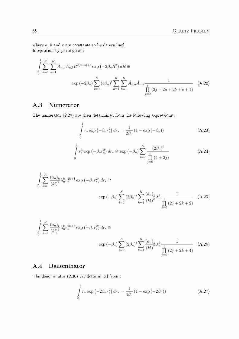
88 Graetz Problem
where a, b and c are constants to be determined.Integration by parts gives :
1∫0
K∑a=1
K∑b=1
An,aAn,bR2(a+b)+c exp
(−2βnR2
)dR ∼=
exp (−2βn)S∑
i=0
(4βn)iK∑
a=1
K∑b=1
An,aAn,b1
i∏j=0
(2j + 2a + 2b + c + 1)(A.22)
A.3 Numerator
The numerator (2.29) are then determined from the following expressions :
1∫0
r∗ exp(−βnr2
∗)dr∗ =
12βn
(1− exp (−βn)) (A.23)
1∫0
r3∗ exp
(−βnr2
∗)dr∗ ∼= exp (−βn)
S∑i=0
(2βn)i
i∏j=0
(4 + 2j)(A.24)
1∫0
K∑k=1
(an)k
(k!)2λk
nr2k+1∗ exp
(−βnr2
∗)dr∗ ∼=
exp (−βn)S∑
i=0
(2βn)iK∑
k=1
(an)k
(k!)2λk
n
1i∏
j=0(2j + 2k + 2)
(A.25)
1∫0
K∑k=1
(an)k
(k!)2λk
nr2k+3∗ exp
(−βnr2
∗)dr∗ ∼=
exp (−βn)S∑
i=0
(2βn)iK∑
k=1
(an)k
(k!)2λk
n
1i∏
j=0(2j + 2k + 4)
(A.26)
A.4 Denominator
The denominator (2.30) are determined from :
1∫0
r∗ exp(−2βnr2
∗)dr∗ =
14βn
(1− exp (−2βn)) (A.27)

A.4 Denominator 89
1∫0
r3∗ exp
(−2βnr2
∗)dr∗ ∼= exp (−2βn)
S∑i=0
(4βn)i
i∏j=0
(4 + 2j)(A.28)
2
1∫0
K∑k=1
(an)k
(k!)2λk
nr2k+1∗ exp
(−2βnr2
∗)dr∗ ∼=
2 exp (−2βn)S∑
i=0
(4βn)iK∑
k=1
(an)k
(k!)2λk
n
1i∏
j=0(2j + 2k + 2)
(A.29)
2
1∫0
K∑k=1
(an)k
(k!)2λk
nr2k+3∗ exp
(−2βnr2
∗)dr∗ ∼=
2 exp (−2βn)S∑
i=0
(4βn)iK∑
k=1
(an)k
(k!)2λk
n
1i∏
j=0(2j + 2k + 4)
(A.30)
1∫0
K∑k=1
((an)k
(k!)2λk
nr2k+ 1
2∗
)2
exp(−2βnr2
∗)dr∗ ∼=
exp (−2βn)S∑
i=0
(4βn)iK∑
k=1
K∑b=1
(an)k
(k!)2λk
n
(an)b
(b!)2λb
n
1i∏
j=0(2j + 2k + 2b + 2)
(A.31)
1∫0
K∑k=1
((an)k
(k!)2λk
nr2k+ 3
2∗
)2
exp(−2βnr2
∗)dr∗ ∼=
exp (−2βn)S∑
i=0
(4βn)iK∑
k=1
K∑b=1
(an)k
(k!)2λk
n
(an)b
(b!)2λb
n
1i∏
j=0(2j + 2k + 2b + 4)
(A.32)

90 Graetz Problem
A.5 Cup Mixing Temperature
The cup mixing temperature for incompressible �ow is :
Tcup−mix =
∫A
uTdA∫A
udA(A.33)
Considering laminar �ow, we replace u with the Poiseuille pro�le given by (2.1), deriving :
Tcup−mix =4r4o
ro∫0
r(r2o − r2
)Tdr (A.34)
Transforming (A.34) on dimensionless form, and introducing the dimensionless variables(see (2.5) and (2.53) as well) :
r∗ =r
roT ∗ =
Tw − T
Tw − Toand T ∗cup−mix =
Tw − Tcup−mix
Tw − To(A.35)
Note for the instance that r∗ are used instead of r∗; only a di�erence of notation. The cup-mixing temperature on dimensionless form is then :
T ∗cup−mix = 4
1∫0
r∗(1− r∗2
)T ∗dr∗ (A.36)
Replacing T ∗ with the dimensionless temperature solution of Graetz problemT ∗Graetz (2.38) gives :
T ∗Graetz−cup−mix = 4
1∫0
∞∑n=0
An exp(−λ2
nx∗)r∗ exp
(−βnr2
∗)dr∗+
4
1∫0
∞∑n=0
An exp(−λ2
nx∗) K∑
k=1
(an)k
(k!)2λk
nr∗2k+1 exp(−βnr2
∗)dr∗−
4
1∫0
∞∑n=0
An exp(−λ2
nx∗)r∗3 exp
(−βnr2
∗)dr∗−
4
1∫0
∞∑n=0
An exp(−λ2
nx∗) K∑
k=1
(an)k
(k!)2λk
nr∗2k+3 exp(−βnr2
∗)dr∗
(A.37)
We evaluate the four terms of the dimensionless cup mixing temperature (A.37) in the samematter as we did for the terms of the coe�cients An.

A.5 Cup Mixing Temperature 91
The result is :
T ∗Graetz−cup−mix = 4∞∑
n=0
An exp(−λ2nx)
(1− exp(−βn))2βn
+ 4∞∑
n=0
An exp(−λ2n)
S∑i=1
(2βn)iK∑
k=1
(an)k
(k!)2λk
n
exp(−βn)i∏
j=0(2k + 2 + 2j)
− 4∞∑
n=0
An exp(−λ2nx)
S∑i=0
(2βn)i exp(−βn)i∏
j=0(4 + 2j)
− 4∞∑
n=0
An exp(−λ2n)
S∑i=1
(2βn)iK∑
k=1
(an)k
(k!)2λk
n
exp(−βn)i∏
j=0(2k + 4 + 2j)
(A.38)

92 Graetz Problem

Appendix B
Turbulent Flow and Heat Transfer
The energy equation for stationary turbulent and incompressible �ow in a pipe is (by ignoringdissipation and axial heat conduction) :
(V + v′x)
∂
∂x
(T + T
′)
+ v′r
∂
∂r
(T + T
′)
+ v′θ
1r
∂
∂θ
(T + T
′)
=k
ρCp
1r
∂
∂r
(r
∂
∂r
(T + T
′))(B.1)
Continuity :
1r
∂
∂r
(rv
′r
)+
1r
∂v′θ
∂θ+
∂v′x
∂x= 0 (B.2)
The Reynolds time averaged energy equation, with typically V � v′x :
V∂T
∂x=
k
ρCp
1r
(r∂T
∂r
)− v′
x
∂T ′
∂x− v′
r
∂T ′
∂r− v
′θ
1r
∂T ′
∂θ(B.3)
Reynolds time averaging the product of the continuity equation multiplied with the �uctuatingvelocity and rewriting gives :
∂
∂r(v′
rT′) +
∂
∂θ
(1rv′θT
′)
+∂
∂x(v′
xT ′) +v′rT
′
r− v′
r
∂T ′
∂r− v
′θ
1r
∂T ′
∂θ− v′
x
∂T ′
∂x= 0 (B.4)
In (B.4) we neglect the terms ∂∂x(...) and ∂
∂θ (...) assuming fully developed �ow. By combining(B.4) with (B.3) we obtain the energy equation :
V∂T
∂x=
k
ρCp
1r
∂
∂r
(r∂T
∂r
)− 1
r
∂
∂r
(rv′
rT′)
(B.5)
Further, we de�ne the thermal eddy-di�usivity by modelling the �uctuating temperature trans-ported in the radial direction :
− v′rT
′ = κt∂T
∂r(B.6)
which, introduced into equation (B.5) give :
V∂T
∂x=
1r
∂
∂r
(r
∂
∂r(κ + κt)
∂T
∂r
)(B.7)

94 Turbulent Flow and Heat Transfer
We will manipulate B.7 by using the de�ned cup-mixing temperature Tcup−mix and the de�nedmass �ux Qm :
2πCp
ro∫0
ρV ∂T∂x rdr
2πro∫0
ρV rdr
=2π∫ ro
0∂∂r
((k + kt) r ∂T
∂r
)dr
2πro∫0
ρV rdr
(B.8)
Notice that k in (B.8) is the thermal conductivity while κ in (B.7) is the thermal di�usivity.By carry out the integration of (B.8) we get :
∂Tcup.mix
∂x= −2πroqw
CpQm(B.9)
B.1 Heat Conduction Through Concentric Walls
Figure B.1: Radial heat �ux through a concentric element
The (radial) heat �ux which streams into the element (see B.1) must equal the (radial)heat �ux leaving the element :
q(r)A(r)− q(r + ∆r)A(r + ∆r) = 0 (B.10)
Letting ∆r− > 0 and rewriting (B.10), we get :
d
dr(rq(r)) = 0 (B.11)
Integration of (B.11) gives :rq(r) = r1qw (B.12)
where qw is the heat �ux found at the inner wall of radius r1, see B.2.Substituting Fourer`s law into (B.12) gives :
− kfr∂T
∂r= r1qw (B.13)
where kf is the thermal conductivity of the �uid in the inner pipe.

B.1 Heat Conduction Through Concentric Walls 95
Figure B.2: Heat conduction through uniform concentric layers
Further integration between two arbitrary concentric layers (see Figure B.2) gives :
Tn−1 = Tn +r1qw
knln
(rn
rn−1
)(B.14)
Notice that we have replaced rnqn with r1qw from (B.12). We use the Newton's law of coolingto evaluate the temperature di�erence between the inner wall and the �uid, or the outer walland the environmental temperature. The temperature di�erence between the inner wall T1
and the bulk �ow Tb is (see B.2) :
(T1 − Tb) =qw
hf(B.15)
where hf is the heat transfer coe�cient of the �uid. The temperature di�erence between theouter wall TN and the environmental temperature is :
(Te − Tb) =1
hN
r1qw
rN(B.16)
where we have replaced qn with r1qw
rNusing (B.12). We can now add the temperature di�erences
to evaluate Te − Tb :
Te − Tb = qo
(1hf
+N∑
n=2
r1
knln(
rn
rn−1
)+
r1
rN
1hN
)(B.17)
If we now introduce the overall heat transfer coe�cient Utot = qw
Te−Tband rewrite (B.17), we
get a general expression for Utot :
Utot =
(1hf
+N∑
n=2
r1
knln(
rn
rn−1
)+
r1
rN
1hN
)−1
(B.18)
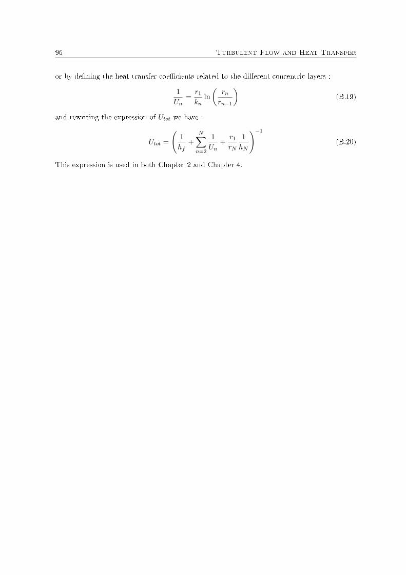
96 Turbulent Flow and Heat Transfer
or by de�ning the heat transfer coe�cients related to the di�erent concentric layers :
1Un
=r1
knln(
rn
rn−1
)(B.19)
and rewriting the expression of Utot we have :
Utot =
(1hf
+N∑
n=2
1Un
+r1
rN
1hN
)−1
(B.20)
This expression is used in both Chapter 2 and Chapter 4.

Appendix C
Experiments
C.1 Isothermal Data
Table C.1: Isothermal Experiments 2007
Month-Year Toil = Twater [oC] Qoil [m3
h ] ∆P [mPa] ρoil [ kgm3 ]
Nov-2007 40 30.00 110.97 801Nov-2007 40 24.99 79.64 801Nov-2007 40 20.00 53.65 801Nov-2007 40 17.50 42.46 801Nov-2007 40 15.04 32.62 801Nov-2007 40 9.98 16.10 801Nov-2007 40 4.99 4.85 801Nov-2007 40 15.00 32.44 801Nov-2007 40 3.45 2.62 801Nov-2007 40 4.89 4.68 801Nov-2007 40 7.17 9.01 801Nov-2007 40 10.06 16.09 801Nov-2007 40 15.19 33.18 801Nov-2007 40 19.96 53.52 801Nov-2007 40 24.98 79.35 801Nov-2007 40 29.99 109.89 801Nov-2007 30 3.56 2.86 808Nov-2007 30 5.31 5.66 808Nov-2007 30 10.05 17.01 808Nov-2007 30 15.19 35.05 808Nov-2007 30 20.00 56.65 808Nov-2007 30 24.99 83.75 808Nov-2007 30 29.99 115.76 808

98 Experiments
Table C.2: Isothermal Experiments 2008
Month-Year Toil = Twater [oC] Qoil [m3
h ] ∆P [mPa] ρoil [ kgm3 ]
Jan-2008 60 29.88 104.3 792Jan-2008 60 25.09 75.82 792Jan-2008 60 20.07 51.02 792Jan-2008 60 15.05 30.50 792Jan-2008 60 10.15 15.68 795Jan-2008 60 5.19 4.88 803Jan-2008 60 24.85 74.83 792Jan-2008 60 16.03 34.88 792Mar-2008 40 30.02 113.39 806Mar-2008 40 25.00 81.84 806Mar-2008 40 20.02 55.07 806Mar-2008 40 15.00 33.47 806Mar-2008 40 10.00 16.37 806Mar-2008 40 5.00 4.97 806Mar-2008 40 20.97 59.87 806Mar-2008 30 29.98 118.17 812Mar-2008 30 25.00 85.78 812Mar-2008 30 20.01 57.98 812Mar-2008 30 15.01 35.00 812Mar-2008 30 10.01 17.31 812Mar-2008 30 4.99 5.31 812Mar-2008 30 21.01 63.14 812Feb-2008 30 21.38 64.67 811Feb-2008 30 29.97 117.48 811Feb-2008 30 25.01 85.29 811Feb-2008 30 20.00 57.57 811Feb-2008 30 15.01 34.86 811Feb-2008 30 10.00 17.19 811Feb-2008 30 5.00 5.23 811Jan-2008 20 29.93 126.86 819Jan-2008 20 25.17 93.53 819Jan-2008 20 20.10 63.19 820Jan-2008 20 15.13 38.81 820Jan-2008 20 10.03 19.01 820Jan-2008 20 5.01 5.68 823Jan-2008 20 24.97 92.04 820Feb-2008 20 30.03 125.15 818Feb-2008 20 24.76 89.26 818Feb-2008 20 20.04 61.51 818Feb-2008 20 15.00 37.27 818Feb-2008 20 10.03 18.48 818Feb-2008 20 4.99 5.43 818Mar-2008 15 25.00 97.09 824Mar-2008 15 20.00 65.94 824Mar-2008 15 14.99 40.09 824Mar-2008 15 10.03 20.19 824Mar-2008 15 5.00 6.12 824Mar-2008 15 20.99 71.73 824

C.2 Non-Isothermal Data 99
C.2 Non-Isothermal Data
Table C.3: Non-Isothermal Experiments 2008
Month-Year Toil [oC] Twater [oC] Qoil [m3
h ] ∆P [mPa] ρoil [ kgm3 ]
Mar-2007 40 10 20.99 62.38 808Mar-2007 30 20 21.00 64.14 813Feb-2007 30 10 21.00 64.40 812Feb-2007 20 10 5.00 6.01 818Mar-2007 15 10 20.99 72.55 824Des-2007 20 12 15.00 43.86 814Jan-2008 20 10 24.93 93.53 820Feb-2008 30 9 21.00 64.51 812Mar-2008 40 10 21.00 62.43 808Mar-2008 15 10 21.00 72.55 824Jan-2008 21 10 21.45 65.20 817Jan-2008 21 12 10.05 19.01 816Jan-2008 20 10 5.18 6.36 818

100 Experiments
1 2 3 4 5 6 7x 10
−3
−0.02
0
0.02
0.04
0.06
0.08
0.1
0.12
0.14
0.16
0.18
Volume flow of oil: [m3/s]
Circles : Derived from the first measurement of each wax experiment, assuming a clean pipe. Squares : Derived from separate experiments where no deposition will occure.
∆P
rela
tive
Relative pressure difference based on non−isothermal experiments where n = 0.05
Experiment 20 − 10 − 10
Experiment 20 −10 − 5
Figure C.1: Relative pressure di�erences for non-isothermal �ow

C.3 Best fit of Measured Pressure Drops 101
C.3 Best �t of Measured Pressure Drops
105 110 115 120 125 130 135 1408400
8500
8600
8700
Time [h]
Pressure
dro
p [
Pa]
Toil
= 15 , Twater
= 10 , Qoil
= 21
75 80 85 90 95 100 1054250
4300
4350
4400
Time [h]
Pressure
dro
p [
Pa]
Toil
= 20 , Twater
= 10 , Qoil
= 15
60 65 70 75 80 857200
7300
7400
7500
Time [h]
Pressu
re d
rop
[P
a]
Toil
= 20 , Twater
= 10 , Qoil
= 21
42 44 46 48 50 52 54 561.005
1.01
1.015
1.02x 10
4
Time [h]
Pressu
re d
rop
[P
a]
Toil
= 20 , Twater
= 10 , Qoil
= 25
150 160 170 180 190 200 2107100
7200
7300
Time [h]
Pressu
re d
ro
p [
Pa]
Toil
= 30 , Twater
= 10 , Qoil
= 21
200 220 240 260 280 3006400
6600
6800
7000
Time [h]
Pressu
re d
ro
p [
Pa]
Toil
= 40 , Twater
= 10 , Qoil
= 21
Figure C.2: Measured pressure drop and best �t curveThe red line shows the best �t line (D) from least-square analysis.

102 Experiments
C.4 Best �t of Measured Temperature Drops
70 80 90 100 1100.04
0.06
0.08
0.1
Time [h]
Tem
peratu
re d
rop [
oC
]
Toil
= 15 , Twater
= 10 , Qoil
= 21
50 55 60 65 70 75 800.2
0.25
0.3
Time [h]
Tem
peratu
re d
rop [
oC
]
Toil
= 20 , Twater
= 10 , Qoil
= 15
40 45 50 55 60 650.2
0.21
0.22
0.23
Time [h]
Tem
peratu
re d
rop [
oC
]
Toil
= 20 , Twater
= 10 , Qoil
= 21
25 30 35 40 450.19
0.2
0.21
0.22
Time [h]
Tem
peratu
re d
rop [
oC
]
Toil
= 20 , Twater
= 10 , Qoil
= 25
100 110 120 130 140 150 1600.5
0.55
0.6
Time [h]
Tem
peratu
re d
rop [
oC
]
Toil
= 30 , Twater
= 10 , Qoil
= 21
150 160 170 180 190 200 210 2201.68
1.7
1.72
1.74
Time [h]
Tem
peratu
re d
rop [
oC
]
Toil
= 40 , Twater
= 10 , Qoil
= 21
Figure C.3: Measured pressure drop and best �t curveThe blue line shows the best �t line (D) from least-square analysis.

C.5 Best Fit of Wax Thickness Calculations 103
C.5 Best Fit of Wax Thickness Calculations
0 0.05 0.1 0.15 0.2 0.25 0.3 0.35 0.4 0.45 0.5−0.06
−0.04
−0.02
0
0.02
0.04
0.06
0.08
0.1
0.12
Time [h]
Th
ickn
ess o
f w
ax d
ep
ositio
n [
mm
]
Toil
= 20 , Twater
= 10 , Qoil
= 15
Figure C.4: Calculated wax thickness with linear approximation
The regression line is given by : R = −0.0506 + 0.321tand based on the measured thickness in the interval 5min to 30 min.

104 Experiments


106 Program Codes
Appendix D
Program Codes
D.1 Maple
# Codes used to derive graphs presented in Chapter 3
> reset;
> # Intention : Comparing the analytical solution of Graetz problem with the profile based on the integral method, using unused engine oil at 320K
> # The radius [m] on the outside (steel) wall of a smooth pipe:
> r_1 := 0.058;
> # The radius on the inside steel wall:
> r_o := 0.050;
> # The radius available for flow with inside insulation of 0.5mm:
> r_i := 0.0495;
> # The area [m^2] on the inside of the smooth pipe, no insulation:
> A_o := evalf[5](Pi*r_o^2);
> # Assuming the volume flux [m^3/s]( turbulent flow) to be a given constant:
> Q_turb := evalf[5](1/2);
> # Volume flux (laminar flow):
> Q_lam := evalf[5](1/(2*100));
> # The density [kg/m^3] given in the table:
> rho := 871.8;
> # The mass flux [kg/s] (turbulent flow) is:
> F_turb := evalf[5](rho*Q_turb);

D.1 Maple 107
> # The mass flux [kg/s] (laminar flow) is:
> F_lam := evalf[5](rho*Q_lam);
> # The area averaged velocity (turbulent flow) [m/s]:
> V_turb := evalf[5](Q_turb/A_o);
> # The area averaged velocity (laminar flow):
> V_lam := evalf[5](Q_lam/A_o);
> # The kinematic viscosity (from table):
> nu := evalf[5](161*10^(-6));
> # The Reynolds number is:
> R[e] := evalf[5](2*r_o*V_turb/nu);
> # The Prandtl number is given in the table:
> Pr := 1965;
> # The Darcy friction factor:
> f := evalf[5]((0.790*ln(R[e])-1.64)^(-2));
> # The Pethukov Nusselt number:
> Nu_turb :=evalf[5](((f/8)*R[e]*Pr)/... (1.07+12.7*(f/8)^(1/2)*(Pr^(2/3)-1)));
> Nu_lam := evalf[5](3.657);
> # The specific heat at constant pressure [J/kgK] from the table:
> Cp := evalf[5](1.993*10^(3));
> # The thermal conductivity of oil [J/smK] from the table:
> k_f := 0.143;

108 Program Codes
> # The viscosity given in the table:
> mu := 0.141;
> # The thermal conductivity of the pipe wall (Hydro 2007):
> k_w := 22.5;
> # The heat coefficient for laminar fluid without insulation:
> h_lam := evalf[5](k_f*Nu_lam/(2*r_o));
> # The heat coefficient for turbulent flow without insulation:
> h_turb := k_f*Nu_turb/(2*r_o);
> # The heat coefficient for laminar fluid with insulation:
> h_lam_i := evalf[5](k_f*Nu_lam/(2*r_i));
> # The heat coefficient for turbulent flow with insulation:
> h_turb_i := k_f*Nu_turb/(2*r_i);
> # The thermal conductivity of the insulation inside the pipe.
> # The insulation can be associated with the wax where:
> k_i := 2*k_f;
> # The heat transfer coefficient for the wall:
> U_w := k_w/(r_o*ln(r_1/r_o));
> # The heat transfer coefficient for the insulation:
> U_i := k_i/(r_o*ln(r_o/r_i));

D.1 Maple 109
> # The overall heat transfer coefficient for laminar flow, including steel wall only:
> U_lam_w := (1/h_lam)^(-1);
> # The overall heat transfer coefficient for turbulent flow, including steel wall only:
> U_turb_w := (1/h_turb + 1/U_w)^(-1);
> # The overall heat transfer coefficient for laminar flow, including steel wall and insulation:
> U_lam_w_i := (1/h_lam_i + 1/U_i)^(-1);
> # The overall heat transfer coefficient for turbulent flow, including steel wall and insulation:
> U_turb_w_i := (1/h_turb_i + 1/U_i + 1/U_w)^(-1);
> # The dimensionless temperature profile derived for turbulent flow based on the Pethukov Nusselt correlation:
> T_turb_a := x-> evalf[5](exp(-2*r_i*Pi*k_f*Nu_turb*x/... (F_turb*Cp)));
> # The dimensionless temperature profile based on laminar flow (Nusselt number), including pipe wall only:
> T_lam_a := x -> evalf[5](exp(-2*r_o*Pi*k_f*Nu_lam*x/... (F_lam*Cp)));
> # The dimensionless temperature profile based on turbulent flow, including pipe wall only:
> T_turb_b := x -> evalf[5](exp(-4*Pi*r_i^2*U_turb_w*x/... (F_turb*Cp)));
> # The dimensionless temperature profile based on turbulent flow, including insulation and pipe wall:
> T_turb_c := x-> evalf[5](exp(-4*Pi*r_i^2*U_turb_w_i*x/... (F_turb*Cp)));

110 Program Codes
> # The dimensionless temperature profile based on laminar flow, including pipe wall only:
> T_lam_b := x-> evalf[5](exp(-4*Pi*r_o^2*U_lam_w*x/... (F_lam*Cp)));
> # The dimensionless temperature profile based on laminar flow, including insulation and pipe wall:
> T_lam_c := x -> evalf[5](exp(-4*Pi*r_o^2*U_lam_w_i*x/... (F_lam*Cp)));
> # Transforming the physical x to the one used in Graetz problem:
> a := 2*k_f/(rho*Cp*V_lam*2*r_o);
> # The area-averaged Graetz temperature profile (8 first eigenvalues):
> T_Graetz := x -> 0.5811207140*exp(-7.313586808*a*x)+ 0.1337702864*exp(-44.60946178*a*x)+
0.06188452782*exp(-113.9210300*a*x)+ 0.03660743080*exp(-215.2405444*a*x)+ 0.02457468598*exp(-348.5641168*a*x)+ 0.01782201444*exp(-513.8900806*a*x)+ 0.02005425268*exp(-711.2180449*a*x)-
0.000014443214*exp(-940.5522368*a*x)+ 0.008814253414*exp(-1201.918059*a*x)+ 5.5996*10^(-8)*exp(-1495.400594*a*x);
> # The dimensionless cup-mixing temperature based on laminar flow and the dimensionless Graetz temperature (8 first eigenvalues):
> T_m := x -> 0.8190502020*exp(-7.313586808*a*x)+ 0.0975269400*exp(-44.60946178*a*x)+
0.03250393024*exp(-113.9210300*a*x)+ 0.01544014236*exp(-215.2405444*a*x)+ 0.008788433200*exp(-348.5641168*a*x)+ 0.00558385500*exp(-513.8900806*a*x)+ 0.003820188404*exp(-711.2180449*a*x)+ 0.00275656884*exp(-940.5522368*a*x)+ 0.002071232000*exp(-1201.918059*a*x)+ 0.001607635356*exp(-1495.400594*a*x);

D.1 Maple 111

112 Program Codes
D.2 Matlab
function Wax_deposition_20_10_21_Jan_2008()
% Basic codes used to derive the graphs in Chapter 4% Here for a fixed wax experiment (20-10-21)
% The following physical variables and parameters are used in the script:% Volume flow (oil): Q_oil [m³/s] % Volume flow (water): Q_water [m³/s]% Pressure drop in oil pipe: dp [Pa]% Temperature incoming oil: T_oil_in [°C]% Temperature outgoing oil: T_oil_out [°C]% Temperature incoming water: T_water_in [°C]% Temperature outgoing water: T_water_out [°C]% Wax apperance temperature: T_WAT [°C]% Temperature difference: Temp_difference [°C]% Inner wall temperature T_iw [°C]% Density of oil: rho_oil [kg/m³]% Density of water: rho_water [kg/m³]% Length of test pipe: dL [m]% Radius of oil/inner pipe: r_oil_i [m]% Thickness of oil/inner pipe: thickness [m]% Radius of inner jacket: r_water_i [m]% Radius of outer jacket: r_water_o [m]% Radius available for flow in oil pipe: r_i [m]% Calculated thickness of wax: Wax_thickness [m]% Correlation curve of Wax_thickness h [m]% Roughness of wall: eps [m]% Average velocity of oil: v_oil [m/s]% Molecular viscosity of oil: my_oil [kg/sm]% Molecular viscosity of water: my_water [kg/sm]% Molecular viscosity of the wall: my_wall [kg/sm]% Heat capacity of oil: Cp_oil [J/kgK]% Heat capacity of water: Cp_water [J/kgK]% Thermal conductivity of steel: k_steel [J/smK] % Thermal conductivity of oil: k_oil [J/smK]% Thermal conductivity of water: k_water [J/smK]% Thermal conductivity of deposit: k_wax [J/smK]% Reynolds number (oil): Re_oil [1]% Reynolds number (water): Re_water [1]% Prandtl number (oil): Pr_oil [1]% Prandtl number (water): Pr_water [1]% Heat transfer coefficient of oil: h_oil [J/sm²K]% Heat transfer coefficient of water: h_water [J/sm²K]% Heat transfer coefficient of the wall: U_w [J/sm²K]% Calculated heat transfer coefficient of deposit U_i [J/sm²K] % Overall heat transfer coefficient: U_tot [J/sm²K]% Pethukov friction factor: f_p [1]% Darcy friction factor: f_d [1]% Friction factor found from best fit analysis: f [1]% Pethukov Nusselt correlation Nu [1]
% Calling on the xls file and declaring the parameters:% Max_row = 1193data = xlsread('Vale_20_10_21.xls',1,'a6:p1193');

D.2 Matlab 113
Q_oil = data(:,3)/3600;dp = data(:,6);T_oil_in = data(:,7);T_oil_out = data(:,8);% The average oil temperatureT_oil = (T_oil_in+T_oil_out)/2;T_water_in = data(:,10);T_water_out = data(:,11);% The average water temperatureT_water = (T_water_in+T_water_out)/2;% The condensate has a WAT in the interval [45,48], we therefore define :T_WAT = (45+48)/2;Temp_difference = -data(:,9); rho_oil = data(:,13);dL = 5.55;r_oil = 0.0526/2;Steel_thickness = 0.0039;r_water_i = r_oil + Steel_thickness;
% Declaring further variables r_i = zeros(1,length(Q_oil+1));% Initial value of the inner radiusr_i(1) = r_oil;h_oil = r_i;T_iw = r_i;Wax_thickness = r_i;% Initial value of wax thicknessWax_thickness(1) = 0;eps = 0; v_oil = Q_oil/(pi*r_oil^2);% The molecular viscosity of oil is determined from a StatoilHydro functionmy_oil = eta_vale(T_oil);my_wall = r_i;
Cp_oil = 1950;k_steel = 22.5;k_oil = 0.1344;Re_oil = my_wall;Re_oil(1) = v_oil(1)*2*r_oil*rho_oil(1)/my_oil(1);Pr_oil = Cp_oil*my_oil/k_oil;f_p = (0.790*log(Re_oil(1))-1.64)^(-2);Nu = ((f_p/8)*Re_oil(1)*Pr_oil(1))/(1.07+12.7*(f_p/8)^(1/2)*(Pr_oil(1)^(2/3)-1)); h_turb = k_oil*Nu/(2*r_oil);% The heat transfer coefficient of steel wallU_w = k_steel/(r_oil*log(r_water_i/r_oil));% The overall heat transfer coefficientbased on oil and steel wallU_turb_w = (1/h_turb + 1/U_w)^(-1);T_iw(1) = T_oil(1) - U_turb_w/h_turb*(T_oil(1)-T_water(1));% Initialising the viscosity of the fluid at the wallmy_wall(1) = eta_vale(T_iw(1));
% Declaring lower and upper boundaryt_min = 2;t_max = length(Q_oil) + 1; % Declaring the time variable (hours) used in most calculationsT = zeros(1,t_max);T(1) = 0;

114 Program Codes
% Declaring the best fit function found from log-log analysis in Chapter 4h = T;% Initialisingh(1) = 0;% Declaring the correlation vector for the averaged exponential alpha-value% given in Chapter 5Correlation = T;% Declaring the correlation vector based on dimensional analysis in Chapter 5 H_c = T;
%tid = zeros(1,t_max-1);f = T;% Defining the vector for the corrected Pethukov friction factorf_p_corrected = T;U_tot = T;k_wax = T;% Assuming no initial deposit on the wall k_wax(1) = k_oil;% Declaring a relative thermal conductivity of steel and wax (Chapter 4)k_steel_wax = T;k_steel_wax(1) = k_steel;
% Declaring the vectors used in the log-log analysis Time = zeros(t_max-120,1);W = zeros(t_max-120,1);Wax = W;
%The difference-vector between h and correlationDiff = T;
for t = t_min:t_max T(1,t) = 5/60*t - 5/60; Re_oil(t-1) = v_oil(t-1)*2*r_i(t-1)*rho_oil(t-1)/my_oil(t-1); f(t-1) = ((1.8*log10(6.9/Re_oil(t-1)+(eps/… (3.7*2*r_i(t-1)))^1.11))^(-2))*(my_wall(t-1)/my_oil(t-1))^(0.05); h(t) = 10^(-3.73)*T(t)^(0.271); Correlation(t) = 10^(-3.87)*T(t)^(0.347); H_c(t) = (2*r_oil*(my_oil(1)/… (3600*rho_oil(1)*(2*r_oil)^2))^0.347)*(Re_oil(1)^(-0.4))*… (((((T_WAT-T_oil_in(t-1))*T_oil_in(t-1))^(0.5))/… T_water_in(t-1))^(4.2))*T(t)^(0.347); if (T_water_in < T_oil_in) Wax_thickness(t) = r_oil - (rho_oil(t-1)*… Q_oil(t-1)^2*f(t-1)/(4*pi^2*dp(t-1)/dL))^(1/5); r_i(t) = r_oil - Wax_thickness(t); % The Pethukov friction factor corrected for non-isothermal flow f_p_corrected(t-1) = ((0.790*log(Re_oil(t-1))-1.64)^(-2))*… (my_wall(t-1)/my_oil(t-1))^(0.05); Nu(t-1) = ((f_p_corrected(t-1)/8)*Re_oil(t-1)*… Pr_oil(t-1))/(1.07+12.7*(f_p_corrected(t-1)/8)^(1/2)*… (Pr_oil(t-1)^(2/3)-1)); h_oil(t-1) = k_oil*Nu(t-1)/(2*r_i(t-1)); U_tot(t-1) = rho_oil(t-1)*v_oil(t-1)*Cp_oil*… (r_oil-Wax_thickness(t-1))./(2*(T_oil(t-1)-… T_water(t-1))).*(Temp_difference(t-1))/dL; T_iw(t) = T_oil(t-1) - U_tot(t-1)/h_oil(t-1)*(T_oil(t-1)-T_water(t-1)); my_wall(t) = eta_vale(T_iw(t));
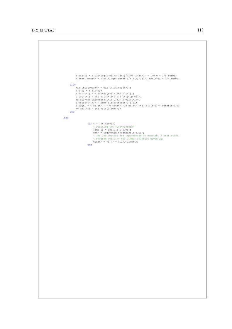
D.2 Matlab 115
k_wax(t) = r_oil*log(r_oil/r_i(t))/(1/U_tot(t-1) - 1/U_w - 1/h_turb); k_steel_wax(t) = r_oil*log(r_water_i/r_i(t))/(1/U_tot(t-1) - 1/h_turb); else Wax_thickness(t) = Wax_thickness(t-1); r_i(t) = r_i(t-1); h_oil(t-1) = k_oil*Nu(t-1)/(2*r_i(t-1)); U_tot(t-1) = rho_oil(t-1)*v_oil(t-1)*Cp_oil*… (r_oil-Wax_thickness(t-1))./(2*(T_oil(t-1)-… T_water(t-1))).*(Temp_difference(t-1))/dL; T_iw(t) = T_oil(t-1) - U_tot(t-1)/h_oil(t-1)*(T_oil(t-1)-T_water(t-1)); my_wall(t) = eta_vale(T_iw(t)); end
end
for t = 1:t_max-120 % Defining the "Log-vectors" Time(t) = log10(T(t+120)); W(t) = log10(Wax_thickness(t+120)); % The log vectors are implemented in Minitab, a statistical % program deriving the linear relation given as: Wax(t) = -3.73 + 0.271*Time(t); end

116 Program Codes
%hold on%plot(Time,Del_Temp,'r');%plot(Time,Wax,'b')%hold off
%hold on%subplot(3,1,2);%plot(T,dp,'b');%plot(T,1000*Wax_thickness,'c');%plot(T,1000*Wax_thickness,'b',T,1000*h,'r');%plot(T,1000*Wax_thickness,'b',T,1000*H_c,'r');%plot(Time,W,'c');%plot(Time,Wax,'r');%plot(T,k_wax/k_oil,'r');%plot(T,h,'r');%xlabel('Time [h]');%ylabel('Wax Thickness [mm]');%title('Best fit of calculated wax thickness: - During the first five hours of the experiment.');%legend('T_{oil} = 20 , T_{water} = 10 , Q_{oil} = 21','Best Fit');%hold off
%hold on%subplot(3,2,6);%plot(T,T_iw,'r');%xlabel('Time [h]');%ylabel('T_{iw} [^oC]');%title('Inner wall temperature');%legend('T_{oil} = 20 , T_{water} = 10 , Q_oil = 21');%hold off
% From Dimensional Analysis%2*r_oil*(my_oil(1)/(3600*rho_oil(1)*(2*r_oil)^2))^0.347%Re_oil(1)%40/T_oil_in(1)

List of Figures
1.1 A completely blocked pipe from the Norwegian shelf . . . . . . . . . . . . . . . 41.2 Wax almost blocking the pipe . . . . . . . . . . . . . . . . . . . . . . . . . . . . 5
2.1 Illustration of Graetz Problem . . . . . . . . . . . . . . . . . . . . . . . . . . . . 92.2 T ∗ when x∗ = 0 . . . . . . . . . . . . . . . . . . . . . . . . . . . . . . . . . . . . 162.3 T ∗ when x∗ = 1
1000 . . . . . . . . . . . . . . . . . . . . . . . . . . . . . . . . . . 162.4 T ∗ when x∗ = 1
100 . . . . . . . . . . . . . . . . . . . . . . . . . . . . . . . . . . . 162.5 T ∗ when x∗ = 1
10 . . . . . . . . . . . . . . . . . . . . . . . . . . . . . . . . . . . 162.6 T ∗ when x∗ = 1
5 . . . . . . . . . . . . . . . . . . . . . . . . . . . . . . . . . . . . 162.7 T ∗ when x∗ = 1
4 . . . . . . . . . . . . . . . . . . . . . . . . . . . . . . . . . . . . 162.8 Stationary Turbulent Flow with Heat Exchange to the Environments . . . . . . 172.9 Turbulent Velocity Pro�le . . . . . . . . . . . . . . . . . . . . . . . . . . . . . . 182.10 In�uence of Pipe Wall Included . . . . . . . . . . . . . . . . . . . . . . . . . . . 202.11 In�uence of Insulation and Pipe Wall . . . . . . . . . . . . . . . . . . . . . . . . 232.12 Localized deposition . . . . . . . . . . . . . . . . . . . . . . . . . . . . . . . . . 25
3.1 Dimensionless cup-mixing temperatures considering laminar �ow . . . . . . . . 303.2 Dimensionless temperature pro�les from the integral method . . . . . . . . . . . 313.3 Dimensionless temperature pro�les from the integral method . . . . . . . . . . . 323.4 Inner wall temperatures considering turbulent �ow . . . . . . . . . . . . . . . . 33
4.1 Wax surface . . . . . . . . . . . . . . . . . . . . . . . . . . . . . . . . . . . . . . 354.2 Picture of the facility . . . . . . . . . . . . . . . . . . . . . . . . . . . . . . . . . 364.3 Sketch of the facility . . . . . . . . . . . . . . . . . . . . . . . . . . . . . . . . . 384.4 Details of the test section . . . . . . . . . . . . . . . . . . . . . . . . . . . . . . 384.5 Hydraulic stresses . . . . . . . . . . . . . . . . . . . . . . . . . . . . . . . . . . . 394.6 Error in the calculated pressure drop for isothermal �ow, Tables C.1 and C.2
(see Appendix) . . . . . . . . . . . . . . . . . . . . . . . . . . . . . . . . . . . . 424.7 Error in calculated pressure drop for non-isothermal �ow, Table C.3 (see Ap-
pendix) . . . . . . . . . . . . . . . . . . . . . . . . . . . . . . . . . . . . . . . . 444.8 Minimum value of |∆Erelative| . . . . . . . . . . . . . . . . . . . . . . . . . . . . 444.9 Measured pressure drop during wax deposition . . . . . . . . . . . . . . . . . . 474.10 Measured pressure drop during wax deposition . . . . . . . . . . . . . . . . . . 484.11 Measured pressure drop during wax deposition . . . . . . . . . . . . . . . . . . 494.12 Measured temperature drop during wax deposition . . . . . . . . . . . . . . . . 514.13 Measured temperature drop during wax deposition . . . . . . . . . . . . . . . . 524.14 Inner wall temperature . . . . . . . . . . . . . . . . . . . . . . . . . . . . . . . . 53

118 LIST OF FIGURES
4.15 Inner wall temperature . . . . . . . . . . . . . . . . . . . . . . . . . . . . . . . . 544.16 Calculated thickness of wax deposit . . . . . . . . . . . . . . . . . . . . . . . . . 564.17 Calculated thickness of wax deposit . . . . . . . . . . . . . . . . . . . . . . . . . 574.18 Calculated thickness of wax deposit . . . . . . . . . . . . . . . . . . . . . . . . . 584.19 Calculated thickness of wax deposit . . . . . . . . . . . . . . . . . . . . . . . . . 594.20 All wax thickness calculations . . . . . . . . . . . . . . . . . . . . . . . . . . . . 604.21 Relative inner wall temperature and relative thickness . . . . . . . . . . . . . . 624.22 Wax thickness derived with constant roughness . . . . . . . . . . . . . . . . . . 654.23 Wax thickness derived with constant roughness . . . . . . . . . . . . . . . . . . 654.24 Wax thickness derived with constant roughness. . . . . . . . . . . . . . . . . . . 664.25 Wax thickness derived with variable roughness . . . . . . . . . . . . . . . . . . 664.26 The relative heat conductivity given by (4.30) . . . . . . . . . . . . . . . . . . . 694.27 The relative heat conductivity of wax deposit compared to oil . . . . . . . . . . 694.28 Log-log-scales of the calculated wax thickness . . . . . . . . . . . . . . . . . . . 714.29 Best �t of calculated wax thickness based on log-log analysis . . . . . . . . . . . 724.30 Best �t of calculated wax thickness based on log-log analysis. . . . . . . . . . . 734.31 Best �t of calculated wax thickness based on log-log analysis . . . . . . . . . . . 74
5.1 Best �t of calculated wax thickness based on dimensional analysis. . . . . . . . 805.2 Best �t of calculated wax thickness based on dimensional analysis . . . . . . . . 81
B.1 Radial heat �ux through a concentric element . . . . . . . . . . . . . . . . . . . 94B.2 Heat conduction through uniform concentric layers . . . . . . . . . . . . . . . . 95
C.1 Relative pressure di�erences for non-isothermal �ow . . . . . . . . . . . . . . . 100C.2 Measured pressure drop and best �t curve . . . . . . . . . . . . . . . . . . . . . 101C.3 Measured pressure drop and best �t curve . . . . . . . . . . . . . . . . . . . . . 102C.4 Calculated wax thickness with linear approximation . . . . . . . . . . . . . . . . 103
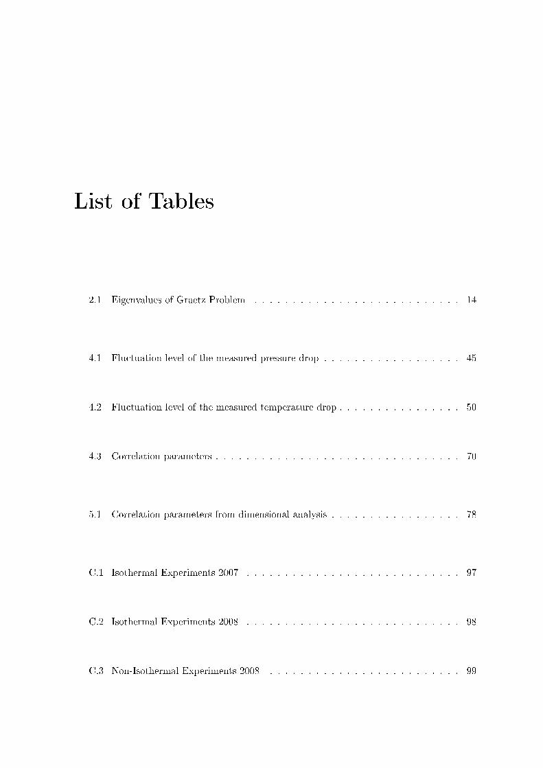
List of Tables
2.1 Eigenvalues of Graetz Problem . . . . . . . . . . . . . . . . . . . . . . . . . . . 14
4.1 Fluctuation level of the measured pressure drop . . . . . . . . . . . . . . . . . . 45
4.2 Fluctuation level of the measured temperature drop . . . . . . . . . . . . . . . . 50
4.3 Correlation parameters . . . . . . . . . . . . . . . . . . . . . . . . . . . . . . . . 70
5.1 Correlation parameters from dimensional analysis . . . . . . . . . . . . . . . . . 78
C.1 Isothermal Experiments 2007 . . . . . . . . . . . . . . . . . . . . . . . . . . . . 97
C.2 Isothermal Experiments 2008 . . . . . . . . . . . . . . . . . . . . . . . . . . . . 98
C.3 Non-Isothermal Experiments 2008 . . . . . . . . . . . . . . . . . . . . . . . . . 99

120 LIST OF TABLES
Nomenclature
u : Laminar flow velocity m
s
V : Area-averaged velocity m
s
: Molecular viscosity kg
sm
: Kinematic viscosity2m
s
k : Thermal conductivity J
smK
: Density3
kg
m
pC : Heat capacity J
kgK
: Thermal diffusivity2m
s
q : Heat flux2
J
sm
h : Heat transfer coefficient of fluid2
J
sm K
U : Heat transfer coefficient2
J
sm K

LIST OF TABLES 121
x : Axial position along pipe m
r : Radius m
T : Temperature K
P : Pressure Pa
: Shear stress Pa
Q : Mass flux kg
s
H : Wax thickness m

122 LIST OF TABLES

Appendix E
Bibliography
Abramowitz, M. and Stegun, I.A., 1964, Handbook of Mathematical Functions, National Bu-reaux of Standards.
Brown T.S., Niesen, V.G. and Erickson, D.D., 1993, "Measurement and Prediction of theKinetics of Para�n Deposition," Society of Petroleum Engineers 26548.
Elphingstone, G.M., Greenhill, K.L. and Hsu, J.J.C., 1999, "Modeling of Multiphase WaxDeposition," Journal of Energy Resources Technology, Vol. 121, pp. 81 - 85.
Graetz, L., 1885, Ann. Physik, Vol. 25, No. 337.
Hausen, H., 1959, "Neue fur die Warmeubertragung bei frir und Erzwungener Stromung,"Allg. Warmetchnik, Vol. 9, pp. 75-79.
Incropera F.P. and DeWitt D.P., 1996, Fundamentals of Heat and Mass Transfer, Fourth
Edition, John Wiley & Sons.
Kok, M.V. and Saracoglu, R.O., 2000, "Mathematical Modelling of Wax Deposition in CrudeOil Pipelines," Petroleum Science and Technology, Vol. 18, No. 9, pp. 1121 - 1145.
Krasovitskii, B.A. and Maron, V.I., 1981, "Growth of Para�n Deposits on the Pipe Wall,"Inzhenerno-Fizichaskii Zhurnal, Vol. 40, No. 4, pp. 683 - 689.
Lee H.S. and Fogler, H.S., 2001, "Combined Convective Heat and Mass Transfer Analysisof Wax Deposition under Turbulent Flow Conditions," Department of Chemical Engineering,
University of Michigan and Chevron Energy Technology Company, Housten.
Lévêque, 1928, Ann. des Mines, Vol. 12, No. 13, pp. 201, 305, 381
Mills, A.F., 1979, Journal of Heat Transfer, Volume 101, Issue 3.
Perry, R.H. and Chilton, C.H., 1973, Chemical Engineer's Handbook, Fifth Edition, McGRAW-HILL.

124 Bibliography
Petukhov, B. S., 1970, "Heat Transfer and Friction in Turbulent Pipe Flow with VariablePhysical Properties," Advances in Heat Transfer, Vol. 6, Academic Press, Inc., New York, pp.504 - 564.
Quarmby, A. and Anand, R.K, 1969, "Axisymmetric Turbulent Mass Transfer in a Circu-lar Tube", J. Fluid Mech., Vol. 38, pp. 433 - 455.
Ramachandran, V. and Fogler, H.S., 2004, "Comments on Analogies for Correlated Heatand Mass Transfer in Turbulent Flow," AIChE, Vol.50, No. 7, pp. 1623 - 1626.
Ramirez-Jaramillo, E., Lira-Galeana, C. and Manero, O., 2004, "Modeling Wax Deposition inPipelines," Petroleum Science and Technology, Vol. 22, No. 7-8, pp. 821 - 861.
Schulkes, R., 2006, "An Introduction to Multiphase Flow", The University of Oslo, Com-
pendium.
Shah, R.K. and London, A.L., 1978, "Laminar Flow Forced Convection in Ducts," Advances
in Heat Transfer, Academic Press.
Singh, P., 2000, "Gel Deposition on Cold Surfaces," The Univeersity of Michigan, PhD Thesis.
Srivastava, S.P., Handoo, J., Agrawal, K.M. and Joshi, G.C., 1993, "Phase-Transition Studiesin n - Alkanes and Petroleum Related Waxes," J. Phys. Chem., Solids, Vol. 54, No. 639.
Svendsen, J.A., 1993, "Mathematical Modeling of Wax Deposition in Oil Pipeline Systems,"AIChE Journal, Vol.39, No. 8, pp. 1377 - 1388.
Todi, S., 2006, "Experimental and Modeling Studies of Wax Deposition in Crude-Oil-CarryingPipelines," O�shore Technology Conference 18368.
Venkatesan, R. and Fogler, H.S., 2004, "Comments on Analogies for Correlated Heat andMass Transfer in Turbulent Flow," AIChe Journal, Vol. 50, No. 7.
White, F.M., 2006, Viscous Fluid Flow, Third Edition, McGRAW-HILL
Wilcox, D.C., 2006, Turbulence Modeling for CFD, Third Edition, DCW Industries


![Prediction of Wax Deposition Risk of Malaysian Crude …11-01-06-004].pdf · International Journal of Science and Advanced Technology (ISSN 2221-8386) Volume 1 No 6 August 2011 89](https://img.pdfslide.us/doc/110x75/5b83e1587f8b9a7d3a8dbdd2/prediction-of-wax-deposition-risk-of-malaysian-crude-11-01-06-004pdf-international.jpg)