Embed Size (px)
Citation preview
Analysis of Runoff from Small Drainage Basins in Wyoming
GEOLOGICAL SURVEY WATER-SUPPLY PAPER 2056
Prepared In cooperation with the Wyoming Highway Department and the U.S. Department of Transportation, Federal Highway Administration
Analysis of Runoff from Small Drainage Basins in Wyoming
By GORDON S. CRAIG, JR., and JAMES G. RANKL
GEOLOGICAL SURVEY WATER-SUPPLY PAPER 2056
Prepared in cooperation with the Wyoming Highway Department and the U.S. Department of Transportation, Federal Highway Administration
UNITED STATES GOVERNMENT PRINTING OFFICE, WASHINGTON : 1978
UNITED STATES DEPARTMENT OF THE INTERIOR
CECIL D. ANDRUS, Secretary
GEOLOGICAL SURVEY
H. William Menard, Director
Library of Congress Catalog-card Number 78-600090
For sale by the Superintendent of Documents, U. S. Government Printing OfEce Washington, D. C. 20402
Stock Number 024-001-03106-0
CONTENTS
Page
Symbols_________________________________________ VAbstract_________________________________________ 1Introduction ________________________________________ 1
Purpose and scope _______ ____________________________ 1 Limitations of study _______________________________ 5Acknowledgments ________________________________________ 5Use of metric units of measurement ________________________ 6
Data collection ____________________________________ 6Description of area __________________________________ 6Instrumentation __________________________________ 7Types of records _________________________________________ 7
Station frequency analysis _________________________________ 9Runoff volume ____ _ ___ ___________________________ 9Rainfall-runoff model---____________________________ 9
Modification of model applied to Wyoming _ ___________ _ _____ 10Use of the model ___________________________________ 13
Transfer of long-term rainfall data _________________________ 16Transfer of long-term evaporation data ___________________ 21
Regional frequency analysis ____________________________ 22Basin characteristics ________ ___ _____________ ________ 24Regression analysis ______________________________ 26
Relation of peak discharge to runoff volume ______________________ 45Other runoff parameters ______________________________ 48Comparison of results ___ ___________________________ 48
Mean dimensionless hydrograph _ _________________ ___ _______ 49Composite mean dimensionless hydrograph __________________ 50Description of the method-________________________ 51Selected comparisons _____ ___ ___ _ _______________ ___ 53
Ponding behind highway embankments _ _ ___________ _____________ _ 55Embankment storage _______ ___ __ _ _____ _______________ 55Method of analysis __________________________________ 57
Application of results.._________________________________ 65Limitations ________________________________________ 66Summary and conclusions ________________________________ 68Selected references __________________________________ 69
III
IV CONTENTS
ILLUSTRATIONS
Page
FIGURE 1. Index map of Wyoming showing locations of 49 small basins studied 4 2. Example of graphical record from a stage-rainfall recording instrument 8
3-5. Graphs showing:3. Relation which determines rainfall excess as a function of
maximum-infiltration capacity and supply rate of rainfall _ _ 114. Relation of rate of decay of CK to time ______________ 125. Variations in the relation which determines rainfall excess as a
function of maximum-infiltration capacityand the supply rate of rainfall ______________________________ 14
6. Map of Wyoming showing the locations of Weather Bureau stations used in the comparison of seasonal precipitation to annual precipitation _____________________________ 20
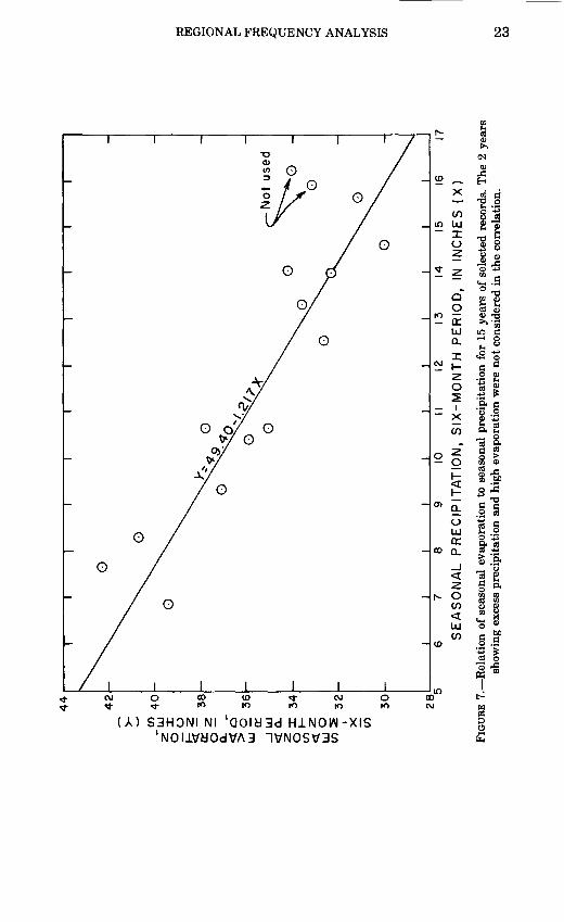
7. Graph showing relation of seasonal evaporation to seasonal precipita tion for 15 years of selected records ____________ ______ _ 23
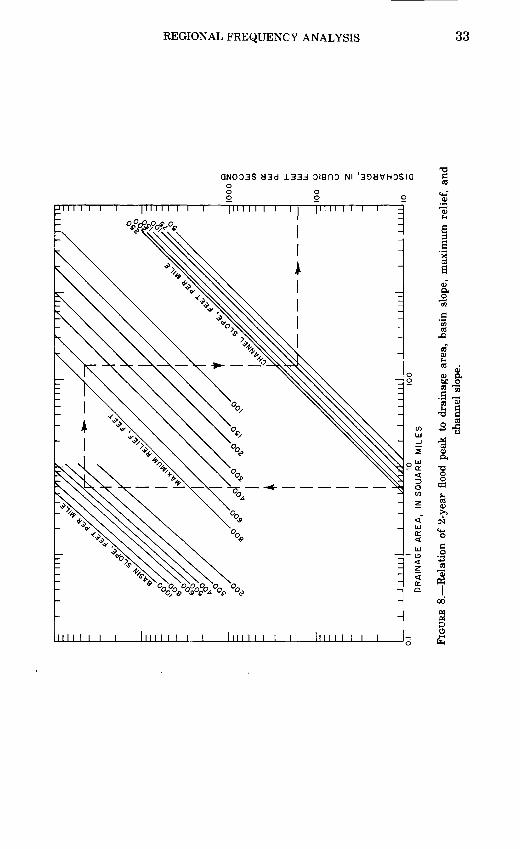
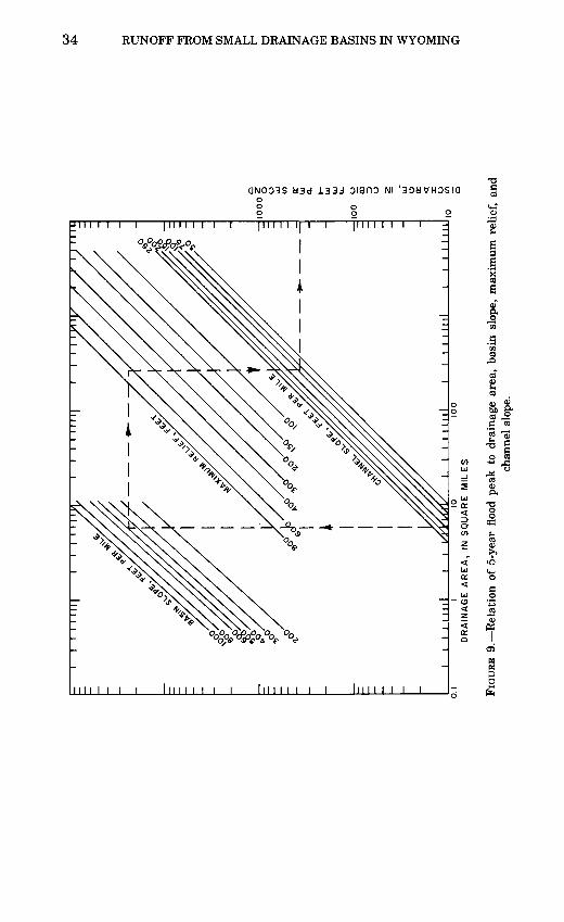
8-13. Graphs showing relation of flood peaks to basin characteristics:8. Relation of 2-year flood peak ___ ______ ____ ____ _ 339. Relation of 5-year flood peak _____________________ 34
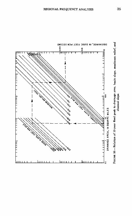
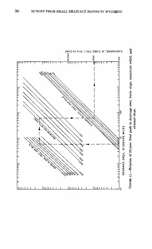
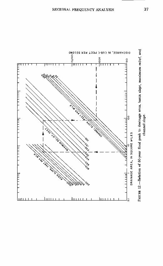
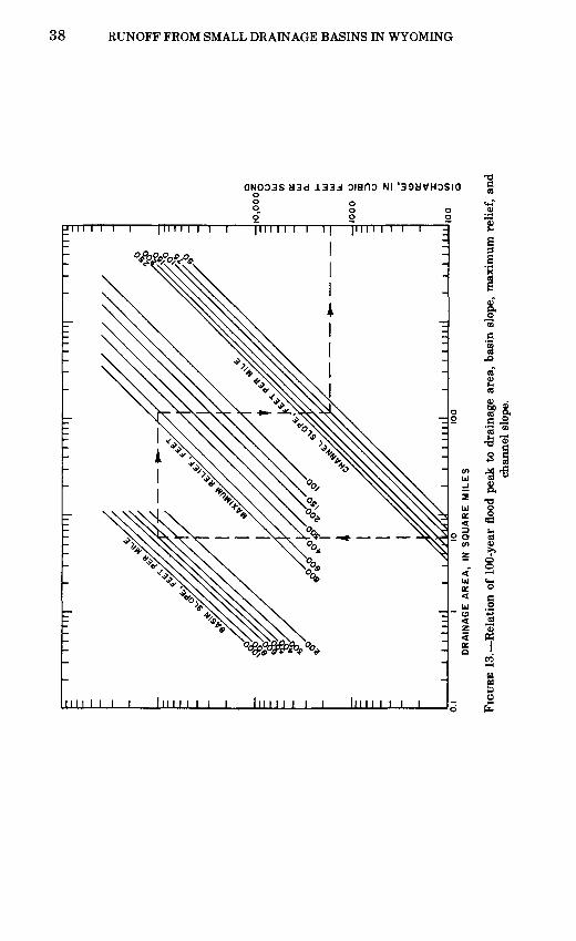
10. Relation of 10-year flood peak __________________ 3511. Relation of 25-year flood peak ___________________ 3612. Relation of 50-year flood peak ____________________ 3713. Relation of 100-year flood peak ____________________ 38
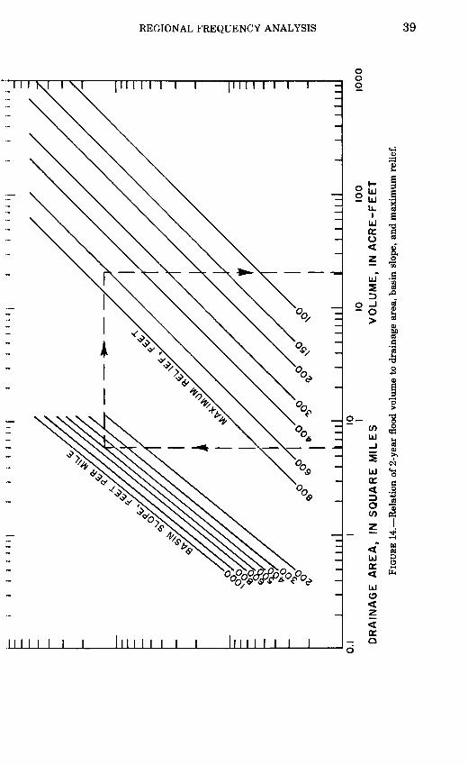
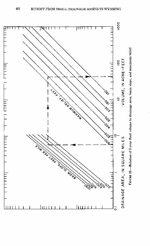
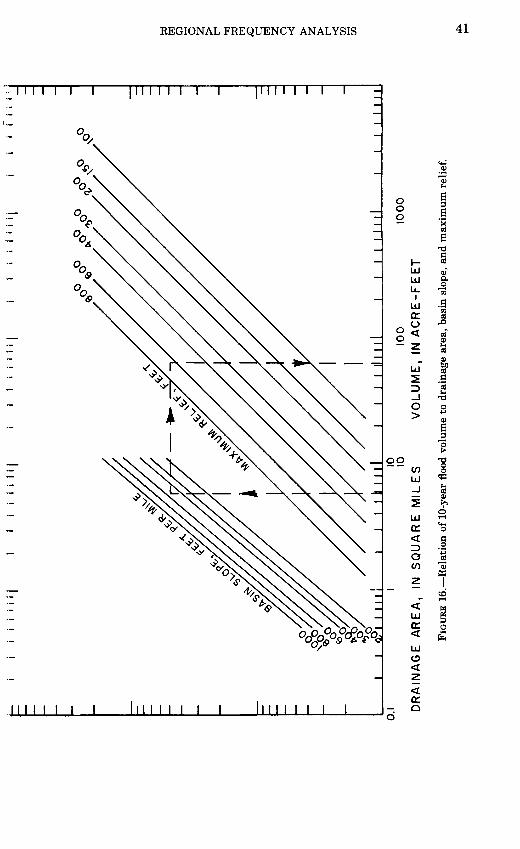
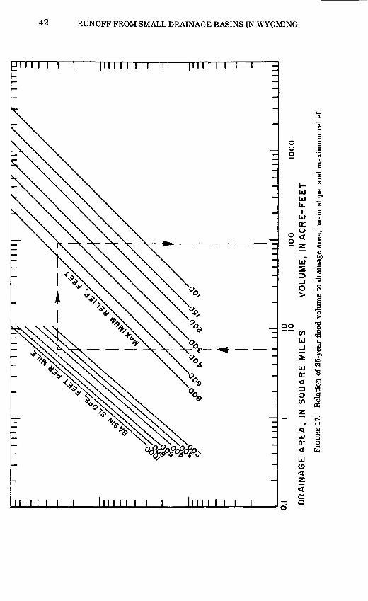
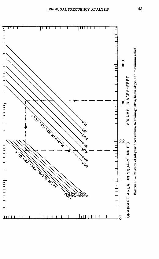
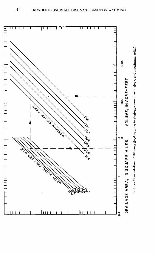
14-19. Graphs showing relation of flood volumes to basin characteristics:14. Relation of 2-year flood volume ___________________ 3915. Relation of 5-year flood volume _________ 4016. Relation of 10-year flood volume ____________________ 4117. Relation of 25-year flood volume __________________ 4218. Relation of 50-year flood volume _____ ______ _ 4319. Relation of 100-year flood volume _____________________ 44
20. Graph showing relation of runoff volume to peak discharge _____ 4621. Composite mean dimensionless hydrograph _____________ 51
22-24. Observed and synthetic hydrographs for:22. Pritchard Draw near Lance Creek, Wyo_______________ 5423. Areas in Wyoming _______________________-____ 5524. Runoff occurrences in Arizona and New Mexico ___________ 56
25. Schematic representation of wedge-shaped ponding area with box- culvert relief _______________________________ 57
26. Culvert discharge rating curves for the culvert sizes investigated __ 60 27-29. Comparison of a natural double-peak runoff hydrograph to a synthe
sized single-peak hydrograph of the same magnitude and volume when routed through the ponding area and a 4 x 4-foot culvert:
27. Low-head flow condition, peak of June 22, 1967 __________ 6128. High-head flow condition, peak of July 25,1965 __________ 6229. High-head flow condition, peak of June 14, 1967 __________ 63
30. A comparison of single-peak hydrographs of equal magnitude but dif ferent volumes routed through the ponding area and a 4 x 4-foot culvert _________________________________ 64
31. Computations and resultant hydrograph for Hay Draw near Midwest, Wyo ______________________________________________ 67
CONTENTS
TABLES
TABLE 1. Comparison of approximate standard error of estimate of the volumeobjective function as determined from the two models ______ _ 10
2. Optimized values of parameters f, g, and C for four calibrated drainage basins __________________________ _ _ 12
3. Final modeling parameters used in long-term synthesis of runoff volumes __________________________________ 15
4. Modeling parameters used in long-term synthesis of peak discharge 165. Volume frequencies for the 22 modeled basins __ 176. Peak frequencies for the 22 modeled basins __________-_____ 187. Ratios used for transferring long-term rainfall data __ _ _ 198. National Weather Service stations with evaporation data used in this
study_____________________________________229. Characteristics of 22 basins _______________ _ - 25
10. Mathematical model and applicable coefficients for use in determining a design discharge or volume______________ _ - 27
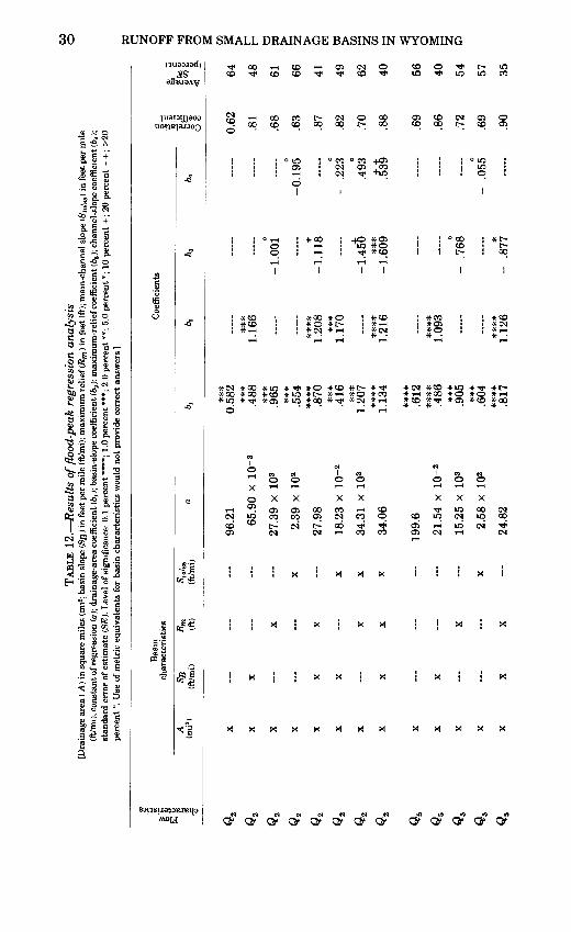
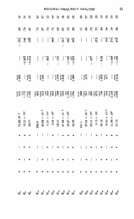
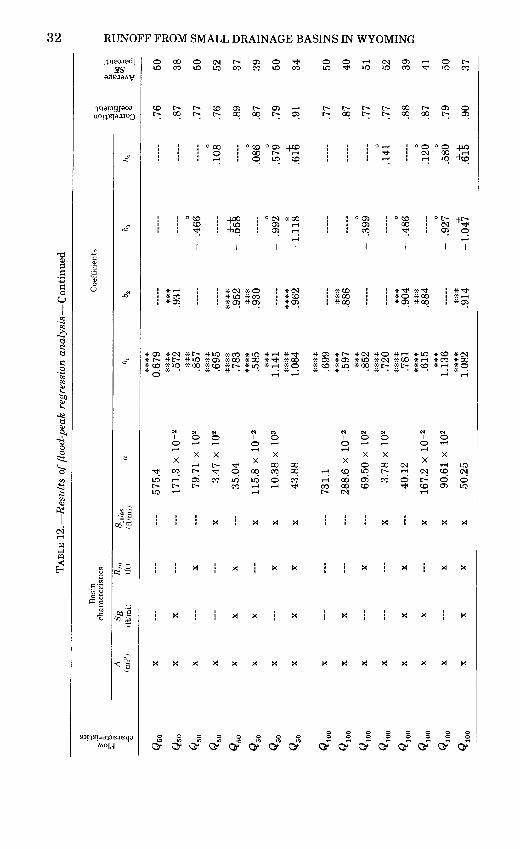
11. Results of flood-volume regression analysis _____ _ ____2812. Results of flood-peak regression analysis ___________ _-_ 3013. Results of two-variable regression on peak discharge and runoff volume 4714. Determination of time, t, and corresponding discharge, q, for points on
the synthetic hydrograph for Pritchard Draw near Lance Creek, Wyoming ____________________________ _-- 53
15. Results of routing single-peak synthetic hydrographs through the var ious reservoir and culvert sizes_________ 59
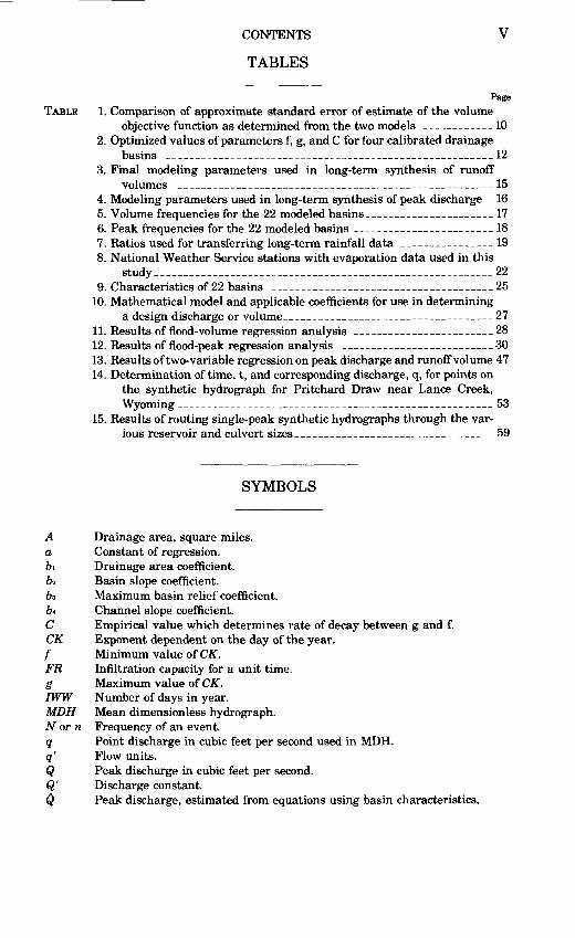
SYMBOLS
A Drainage area, square miles.a Constant of regression.61 Drainage area coefficient.bi Basin slope coefficient.ba Maximum basin relief coefficient.bt Channel slope coefficient.C Empirical value which determines rate of decay between g and f.CK Exponent dependent on the day of the year.f Minimum value ofCK.FR Infiltration capacity for a unit time.g Maximum value of CK.IWW Number of days in year.MDH Mean dimensionless hydrograph.N or n Frequency of an event.q Point discharge in cubic feet per second used in MDH.q' Flow units.Q Peak discharge in cubic feet per second.Q' Discharge constant.0 Peak discharge, estimated from equations using basin characteristics.
VI CONTENTS
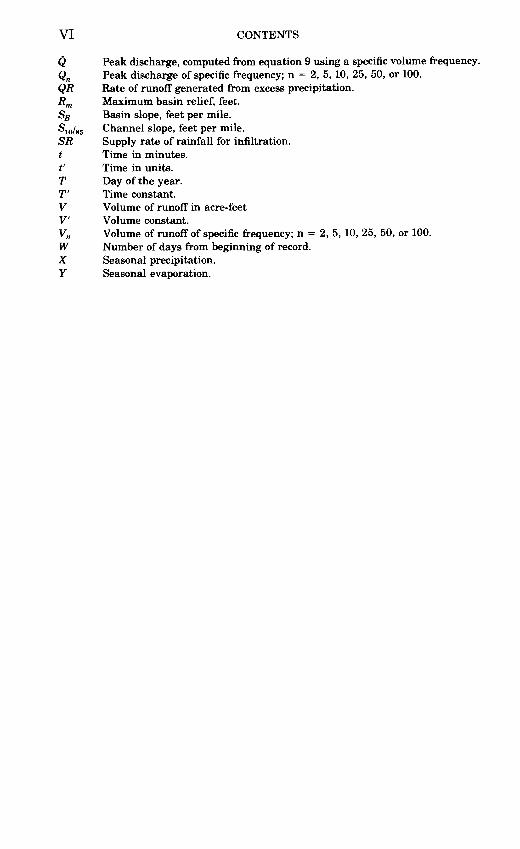
0 Peak discharge, computed from equation 9 using a specific volume frequency.Qn Peak discharge of specific frequency; n = 2, 5, 10, 25, 50, or 100.QR Rate of runoff generated from excess precipitation.Rm Maximum basin relief, feet.Sg Basin slope, feet per mile.S10/85 Channel slope, feet per mile.SR Supply rate of rainfall for infiltration.t Time in minutes.t' Time in units.T Day of the year.T' Time constant.V Volume of runoff in acre-feetV Volume constant.Vn Volume of runoff of specific frequency; n = 2, 5, 10, 25, 50, or 100.W Number of days from beginning of record.X Seasonal precipitation.Y Seasonal evaporation.
ANALYSIS OF RUNOFF FROM SMALL DRAINAGE BASINS IN WYOMING
By GORDON S. CRAIG, JR., and JAMES G. RANKL
ABSTRACT
A flood-hydrograph study has denned the magnitude and frequency of flood volumes and flood peaks that can be expected from drainage basins smaller than 11 square miles in the plains and valley areas of Wyoming. Rainfall and runoff data, collected for 9 years on a seasonal basis (April through September), were used to calibrate a rainfall- runoff model on each of 22 small basins. Long-term records of runoff volume and peak discharge were synthesized for these 22 basins.
Flood volumes and flood peaks of specific recurrence intervals (2, 5, 10, 25, 50, and 100 years) were then related to basin characteristics with a high degree of correlation. Flood volumes were related to drainage area, maximum relief, and basin slope. Flood peaks were related to drainage area, maximum relief, basin slope, and channel slope.
An investigation of ponding behind a highway embankment, with available storage capacity and with a culvert to allow outflow, has shown that the single fast-rising peak is most important in culvert design. Consequently, a dimensionless hydrograph defines the characteristic shape of flood hydrographs to be expected from small drainage basins in Wyoming. For design purposes, a peak and volume can be estimated from basin characteristics and used with the dimensionless hydrograph to produce a synthetic single-peak hydrograph. Incremental discharges of the hydrograph can be routed along a channel, where a highway fill and culvert are to be placed, to help determine the most economical size of culvert if embankment storage is to be considered.
INTRODUCTION
PURPOSE AND SCOPE
Streamflow data have been collected for many years on large per ennial streams in Wyoming and other western states, thus providing information for road and bridge designers. However, very little in formation is available on small ephemeral streams. Because there are more small drainages, than large streams to deal with in most road
2 RUNOFF FROM SMALL DRAINAGE BASINS IN WYOMING
construction projects, they are a major concern to the designer. In 1964 the U.S. Geological Survey, in cooperation with the Wyoming State Highway Department and the Federal Highway Administra tion, initiated a study of flood hydrographs in Wyoming. The purpose was to investigate runoff from small drainage basins, less than 11 square miles, and to develop methods that would be helpful in the design of hydraulic stuctures.
Previous reports concerning the estimation of flow characteristics for Wyoming streams include statewide reports by Carter and Green (1963), Wahl (1970), and Druse and Wahl (written commun., 1972). In addition, a series of published reports that cover entire river basins, parts of which are in Wyoming, include: Thomas, Broom, and Cum- mans (1963), Snake River Basin; Patterson (1966) and Matthai (1968), Missouri River Basin; Patterson and Somers (1966), Colorado River Basin; and Butler, Reid, and Berwick (1966), the Great Basin. These reports are concerned only with the frequencies of flood peaks and are not applicable for use on very small drainage basins. Lowham (1976) has prepared a statewide report on flood-peak frequencies that super sedes the above-mentioned reports. There are no known studies or reports about total storm runoff volumes on ephemeral streams, as presented in this report, that are applicable to streams in Wyoming.
This report provides methods to estimate runoff-volume and flood- peak frequencies for small drainage basins in Wyoming. The area of investigation was confined to the large valleys and plains, where most roads are built and where very little streamflow information is available. The study was made on a seasonal basis (April 1 to Sep tember 30), because this is the period of thunderstorm activity and high-intensity rainfall, which cause the high-runoff events. Snow- melt runoff is usually not significant on small drainage basins at lower elevations although exceptions occasionally are possible.
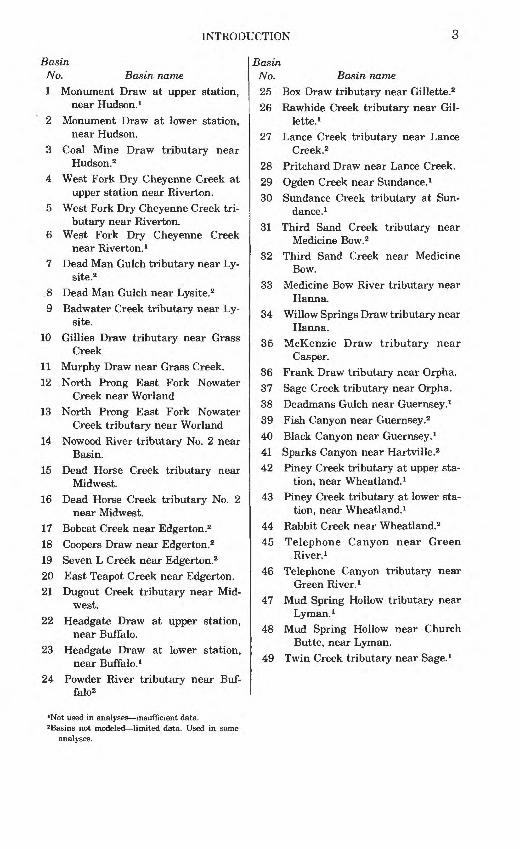
A total of 49 drainage basins were instrumented for this study (fig. 1); 14 of these basins were omitted from the analyses because of in sufficient data. During the 9-year period of record, the number of hy drographs recorded on any one basin ranged from none to as many as 30. Three hydrographs from each of 35 basins were used in the peak discharge-runoff volume study. Seven or more hydrographs from each of 28 basins were used in the study of dimensionless hydrographs. Twelve or more hydrographs, with associated rainfall from each of 22 basins, were used in the calibration of the rainfall-runoff model. The following is a list of the 49 study basins in Wyoming:
INTRODUCTION
Basin No. Basin name
1 Monument Draw at upper station, near Hudson. 1
2 Monument Draw at lower station, near Hudson.
3 Coal Mine Draw tributary near Hudson.2
4 West Fork Dry Cheyenne Creek at upper station near Riverton.
5 West Fork Dry Cheyenne Creek tri butary near Riverton.
6 West Fork Dry Cheyenne Creek near Riverton. 1
7 Dead Man Gulch tributary near Ly- site.2
8 Dead Man Gulch near Lysite.29 Badwater Creek tributary near Ly
site.10 Gillies Draw tributary near Grass
Creek11 Murphy Draw near Grass Creek.12 North Prong East Fork Nowater
Creek near Worland13 North Prong East Fork Nowater
Creek tributary near Worland14 Nowood River tributary No. 2 near
Basin.15 Dead Horse Creek tributary near
Midwest.16 Dead Horse Creek tributary No. 2
near Midwest.17 Bobcat Creek near Edgerton.218 Coopers Draw near Edgerton.219 Seven L Creek near Edgerton.220 East Teapot Creek near Edgerton.21 Dugout Creek tributary near Mid
west.22 Headgate Draw at upper station,
near Buffalo.23 Headgate Draw at lower station,
near Buffalo. 124 Powder River tributary near Buf
falo2
'Not used in analyses insufficient data. 2Basins not modeled limited data. Used in some
analyses.
Basin No. Basin name
25 Box Draw tributary near Gillette.226 Rawhide Creek tributary near Gil
lette. 127 Lance Creek tributary near Lance
Creek.228 Pritchard Draw near Lance Creek.29 Ogden Creek near Sundance. 130 Sundance Creek tributary at Sun-
dance. 131 Third Sand Creek tributary near
Medicine Bow.232 Third Sand Creek near Medicine
Bow.33 Medicine Bow River tributary near
Hanna.34 Willow Springs Draw tributary near
Hanna.35 McKenzie Draw tributary near
Casper.36 Frank Draw tributary near Orpha.37 Sage Creek tributary near Orpha.38 Deadmans Gulch near Guernsey. 139 Fish Canyon near Guernsey.240 Black Canyon near Guernsey. 141 Sparks Canyon near Hartville.242 Piney Creek tributary at upper sta
tion, near Wheatland. 143 Piney Creek tributary at lower sta
tion, near Wheatland. 144 Rabbit Creek near Wheatland.245 Telephone Canyon near Green
River. 146 Telephone Canyon tributary near
Green River. 147 Mud Spring Hollow tributary near
Lyman. 148 Mud Spring Hollow near Church
Butte, near Lyman.49 Twin Creek tributary near Sage. 1
RUNOFF FROM SMALL DRAINAGE BASINS IN WYOMING
III 0 110° 109° 108° (07° 106° (05° (04°---.-4-^--T--;tv^^HlS<
^j-HEYEftlte^*
rrti--"^_riJ -J^4I G
105° 104°
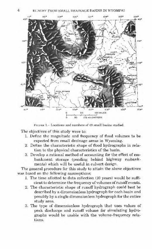
FIGURE 1. Locations and numbers of 49 small basins studied.
The objectives of this study were to:1. Define the magnitude and frequency of flood volumes to be
expected from small drainage areas in Wyoming.2. Define the characteristic shape of flood hydrographs in rela
tion to the physical characteristics of the basin.3. Develop a rational method of accounting for the effect of em
bankment storage (ponding behind highway embank ments) which will be useful in culvert design.
The general procedure for this study to attain the above objectives was based on the following assumptions:
1. The time allotted to data collection (10 years) would be suffi cient to determine the frequency of volumes of runoff events.
2. The characteristic shape of runoff hydrograph could best be described by a dimensionless hydrograph for each basin and possibly by a single dimensionless hydrograph for the entire study area.
3. The type of dimensionless hydrograph that uses values of peak discharge and runoff volume for simulating hydro- graphs would be usable with the volume-frequency rela tions.
INTRODUCTION 5
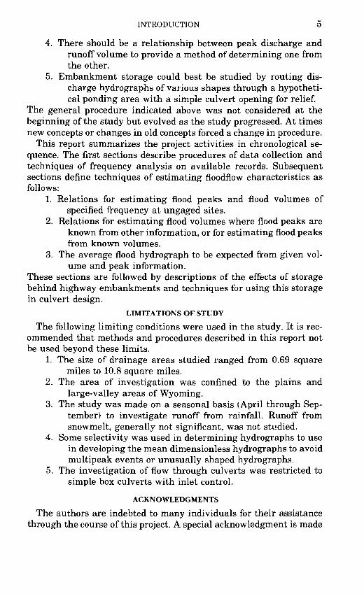
4. There should be a relationship between peak discharge and runoff volume to provide a method of determining one from the other.
5. Embankment storage could best be studied by routing dis charge hydrographs of various shapes through a hypotheti cal ponding area with a simple culvert opening for relief.
The general procedure indicated above was not considered at the beginning of the study but evolved as the study progressed. At times new concepts or changes in old concepts forced a change in procedure.
This report summarizes the project activities in chronological se quence. The first sections describe procedures of data collection and techniques of frequency analysis on available records. Subsequent sections define techniques of estimating floodflow characteristics as follows:
1. Relations for estimating flood peaks and flood volumes of specified frequency at ungaged sites.
2. Relations for estimating flood volumes where flood peaks are known from other information, or for estimating flood peaks from known volumes.
3. The average flood hydrograph to be expected from given vol ume and peak information.
These sections are followed by descriptions of the effects of storage behind highway embankments and techniques for using this storage in culvert design.
LIMITATIONS OF STUDY
The following limiting conditions were used in the study. It is rec ommended that methods and procedures described in this report not be used beyond these limits.
1. The size of drainage areas studied ranged from 0.69 square miles to 10.8 square miles.
2. The area of investigation was confined to the plains and large-valley areas of Wyoming.
3. The study was made on a seasonal basis (April through Sep tember) to investigate runoff from rainfall. Runoff from snowmelt, generally not significant, was not studied.
4. Some selectivity was used in determining hydrographs to use in developing the mean dimensionless hydrographs to avoid multipeak events or unusually shaped hydrographs.
5. The investigation of flow through culverts was restricted to simple box culverts with inlet control.
ACKNOWLEDGMENTS
The authors are indebted to many individuals for their assistance through the course of this project. A special acknowledgment is made
6 RUNOFF FROM SMALL DRAINAGE BASINS IN WYOMING
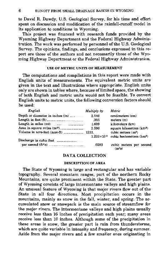
to David R. Dawdy, U.S. Geological Survey, for his time and effort spent on discussion and modification of the rainfall-runoff model in its application to conditions in Wyoming.
This project was financed with research funds provided by the Wyoming Highway Department and the Federal Highway Adminis tration. The work was performed by personnel of the U.S. Geological Survey. The opinions, findings, and conclusions expressed in this re port are those of the authors and not necessarily those of the Wyo ming Highway Department or the Federal Highway Administration.
USE OF METRIC UNITS OF MEASUREMENT
The computations and compilations in this report were made with English units of measurements. The equivalent metric units are given in the text and illustrations where appropriate. English units only are shown in tables where, because of limited space, the showing of both English and metric units would not be feasible. To convert English units to metric units, the following conversion factors should be used:
English Multiply by Metric Depth or diameter in inches (in) _____ 2.540 centimeters (cm) Length in feet (ft) ______________ .305 meters (m) Length in miles (mi) ___________ 1.609 kilometers (km) Area in square miles (mi2)________ 2.590 square kilometers (km2) Volume in acre-feet (acre-ft) _______ 1233. cubic meters (m3 )
1.233 x 10 3 cubic hectometers (hm3) Discharge in cubic feet ______________
per second (ft3/s) _____________ .0283 cubic meters per second(m3s)
DATA COLLECTION
DESCRIPTION OF AREA
The State of Wyoming is large and rectangular and has variable topography. Several mountain ranges, part of the northern Rocky Mountains, are quite prominent within the State. The greater part of Wyoming consists of large intermontane valleys and high plains. An unusual feature of Wyoming is that major rivers flow out of the State in all four directions. Most precipitation occurs in the mountains, mainly as snow in the fall, winter, and spring. The ac cumulated snow or snowpack is the main source of streamflow for the major rivers. The intermontane valleys and high plains usually receive less than 16 inches of precipitation each year; many areas receive less than 10 inches. Although some of the precipitation in these areas is snow, the greater part is rain from thunderstorms, which are quite variable in intensity and frequency, during summer. Aside from the major rivers and a few smaller ones originating in
DATA COLLECTION 7
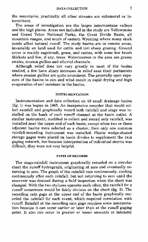
the mountains, practically all other streams are ephemeral or in termittent.
The areas of investigation are the larger intermontane valleys and the high plains. Areas not included in the study are Yellowstone and Grand Teton National Parks, the Great Divide Basin, all mountain ranges, and much of eastern Wyoming where many stock ponds affect natural runoff. The study basins are in remote areas, invariably on land used for cattle and (or) sheep grazing. Ground cover is mainly sagebrush, grass, and cactus, with some low brush thickets and few, if any, trees. Watercourses in the area are grassy swales, erosion gullies and alluvial channels.
Although relief does not vary greatly in most of the basins studied, a few have sharp increases in relief near their perimeters where erosion gullies are quite prominent. The generally open expo sure of the basins to sun and wind result in rapid drying and high evaporation of soil moisture in the basins.
INSTRUMENTATION
Instrumentation and data collection on 49 small drainage basins (fig. 1) was begun in 1965. An inexpensive recorder that would col lect rainfall and graphically record both rainfall and stage was in stalled on the bank of each runoff channel at the basin outlet. A similar instrument, modified to collect and record only rainfall, was installed near the upper end of each basin, except when two or three adjacent basins were selected as a cluster; then only one common rainfall-recording instrument was installed. Plastic wedge-shaped storage gages were placed on basin divides to supplement the rain gaging network, but because interpretation of individual storms was difficult, they were not very helpful.
TYPES OF RECORDS
The stage-rainfall instrument graphically recorded on a circular chart the runoff hydrograph, originating at zero and eventually re turning to zero. The graph of the rainfall rose continuously, circling continuously after each rainfall, but not returning to zero until the reservoir was drained during a field inspection when the chart was changed. With the two styluses opposite each other, the rainfall for a runoff occurrence would be fairly obvious on the chart (fig. 2). The recording rain gage at the upper end of the basin graphically rec orded the rainfall for each event, which required correlation with runoff. Rainfall at the recording rain gage requires some interpreta tion because it can occur earlier or later than at the runoff gaging point. It also can occur in greater or lesser amounts or intensity
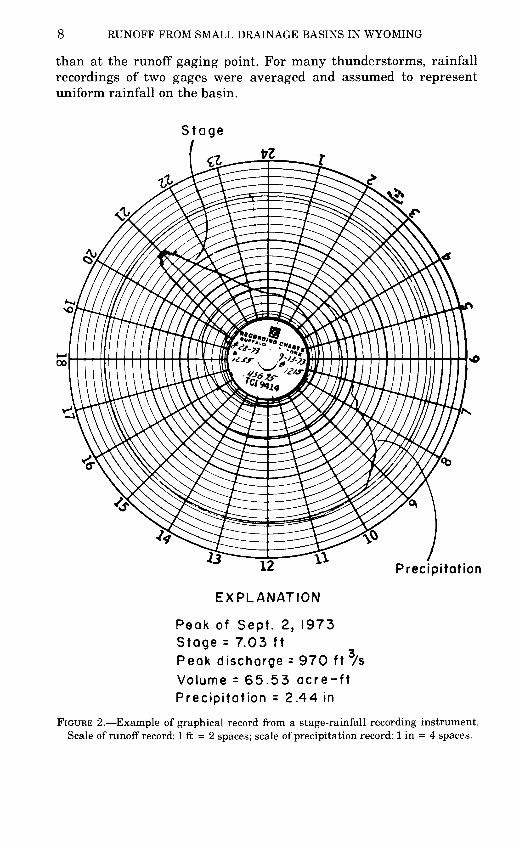
8 RUNOFF FROM SMALL DRAINAGE BASINS IN WYOMING
than at the runoff gaging point. For many thunderstorms, rainfall recordings of two gages were averaged and assumed to represent uniform rainfall on the basin.
Stage
frZ
12 ' Precipitation
EXPLANATION
Peak of Sept. 2, 1973 Stage = 7.03 ft Peak discharge = 970 ft 3/s Volume = 65.53 acre-ft Precipitation = 2.44 in
FIGURE 2. Example of graphical record from a stage-rainfall recording instrument. Scale of runoff record: 1 ft = 2 spaces; scale of precipitation record: 1 in = 4 spaces.
STATION FREQUENCY ANALYSIS 9
Stage-discharge relations were developed by current-meter mea surements of low flows when possible, by indirect measurements of peak flows, and by step-backwater analyses through a range of flows. The remote stations were inaccessible during high flows and had no facilities to allow for direct current-meter measurements of peak flows. Discharge hydrographs were obtained by applying the stage-discharge relations to values of stage picked from the charts at 5-minute increments.
STATION FREQUENCY ANALYSIS
RUNOFF VOLUME
One objective of this study was to define the magnitude and fre quency of flood volumes to be expected from small drainage basins in Wyoming. Data collected for small basins in Wyoming indicated considerable variation in runoff volume from like amounts of point rainfall data, even for the same basin. One problem is that while point rainfall data are projected as uniform rainfall over a basin, in many cases rainfall distribution is not uniform. The assumption of uniform rainfall is considered reasonable because point data can be too high as well as too low and over a period of time it is expected to average out. Usually, the greater volumes occur from the larger total rainfalls, permitting the assumption that the annual maximum runoff volume does result from the annual maximum rainfall occurrence. This is not always correct, however, because other conditions change sufficiently to increase or decrease the runoff volume from a particular rainfall. A procedure for ap proximating changes in conditions within a drainage basin and es timating runoff volume or peak discharge from rainfall has been de veloped and is used in the digital models described in this report.
RAINFALL-RUNOFF MODEL
Rainfall-runoff modeling has been used to synthesize long-term runoff records from long-term rainfall records. The long-term rain fall records are available from National Weather Service stations throughout the United States. Short-term rainfall and runoff data, collected simultaneously on small drainage basins, are used to cali brate the model. Each basin is calibrated separately. Once calib rated, the model utilizes the long-term rainfall record to generate a synthetic long-term runoff record, equivalent in time.
A model developed by D. W. Dawdy, R. W. Lichty, and J. M. Bergmann (1972) was adapted for use in this study. This parametric model originally used seven parameters to simulate physical condi tions in a drainage basin in the process of estimating rainfall excess.
10 RUNOFF FROM SMALL DRAINAGE BASINS IN WYOMING
Four parameters were used to account for antecedent moisture con ditions and three were used to determine infiltration. For this study, three additional parameters were incorporated into the model to ac count for a variation in infiltration with time. This modification, de scribed in the next section, considers a change in soil conditions as a seasonal variation to reduce infiltration, and is applicable in a semiarid region. The interpretation was based on visual observation of a consistent change in soil appearance through each field season and the consideration of many high-runoff events that occurred in late summer.
MODIFICATION OF MODEL APPLIED TO WYOMING
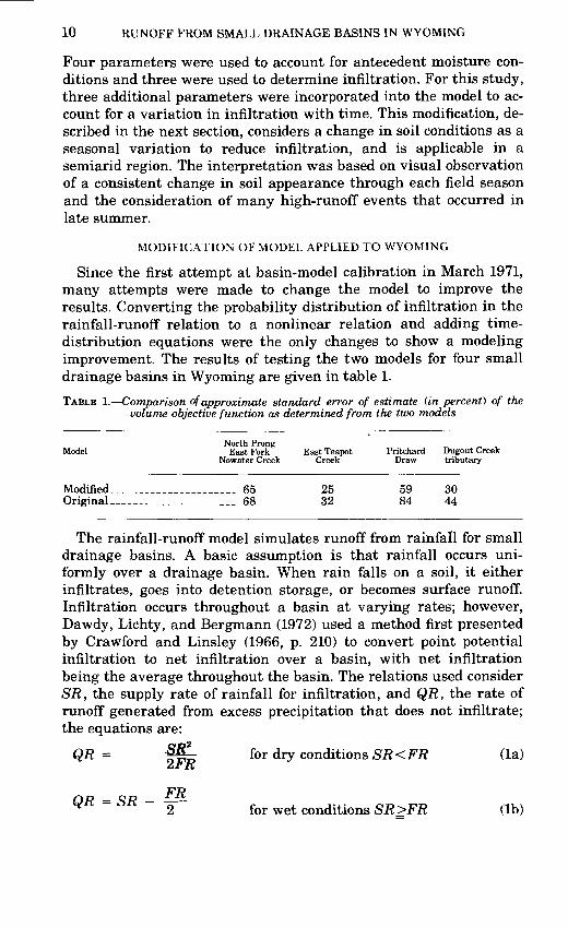
Since the first attempt at basin-model calibration in March 1971, many attempts were made to change the model to improve the results. Converting the probability distribution of infiltration in the rainfall-runoff relation to a nonlinear relation and adding time- distribution equations were the only changes to show a modeling improvement. The results of testing the two models for four small drainage basins in Wyoming are given in table 1.
TABLE 1. Comparison of approximate standard error of estimate (in percent) of the volume objective function as determined from the two models
Model
Modified _ .
North Prong East Fork
Nowater Creek
___ ___ 65_____________ 68
East Teapot Creek
2532
Pritchard Draw
5984
Dugout Creek tributary
3044
The rainfall-runoff model simulates runoff from rainfall for small drainage basins. A basic assumption is that rainfall occurs uni formly over a drainage basin. When rain falls on a soil, it either infiltrates, goes into detention storage, or becomes surface runoff. Infiltration occurs throughout a basin at varying rates; however, Dawdy, Lichty, and Bergmann (1972) used a method first presented by Crawford and Linsley (1966, p. 210) to convert point potential infiltration to net infiltration over a basin, with net infiltration being the average throughout the basin. The relations used consider SR, the supply rate of rainfall for infiltration, and QR, the rate of runoff generated from excess precipitation that does not infiltrate; the equations are:
QR = for dry conditions SR<FR (la) 2JrR
QR =SR - Y~ for wet conditions SR>FR (Ib)
STATION FREQUENCY ANALYSIS 11
0 25 50 75 100PERCENTAGE OF AREA WITH INFILTRATION CAPACITY
EQUAL TO OR LESS THAN INDICATED VALUE
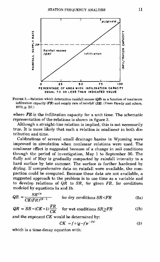
FIGURE 3. Relation which determines rainfall excess (QR) as a function of maximum infiltration capacity (Fft) and supply rate of rainfall (SR). (From Dawdy and others, 1972, p. B7.)
where FR is the infiltration capacity for a unit time. The schematic representation of the relations is shown in figure 3.
Although a straight-line relation is implied, this is not necessarily true. It is more likely that such a relation is nonlinear in both dis tribution and time.
Calibrations of several small drainage basins in Wyoming were improved in simulation when nonlinear relations were used. The nonlinear effect is suggested because of a change in soil conditions through the period of investigation, May 1 to September 30. The fluffy soil of May is gradually compacted by rainfall intensity to a hard surface by late summer. The surface is further hardened by drying. If comprehensive data on rainfall were available, the com paction could be computed. Because these data are not available, a suggested approach to the problem is to use time as a variable and to develop relations of QR to SR, for given FR, for conditions modeled by equations la and Ib.
SR CKfor dry conditions SR<FR (2a)CK-lCK(FR)
QR = SR-(CK-1) FR CK
for wet conditions SR>FR
and the exponent CK would be determined by:CK = f+(g-f)e-TIC
which is a time-decay equation with:
(2b)
(3)
12 RUNOFF FROM SMALL DRAINAGE BASINS IN WYOMING
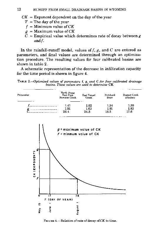
CK = Exponent dependent on the day of the year T = The day of the year f = Minimum value of CK g = Maximum value ofCKC = Empirical value which determines rate of decay between g
and/".
In the rainfall-runoff model, values of f, g, and C are entered as parameters, and final values are determined through an optimiza tion procedure. The resulting values for four calibrated basins are shown in table 2.
A schematic representation of the decrease in infiltration capacity for the time period is shown in figure 4.
TABLE 2. Optimized values of parameters f, g, and C for four calibrated drainage basins. These values are used to determine CK
North Prong Parameter East Fork
Nowater Creek
f ____ _ __ 1.41g ____ __ ______ 1.91C 26.4
East Teapot Creek
1.621.63
24.8
Pritchard Draw
1.341.91
16.5
Dugout Creek tributary
1.301.83
17.6
g - maximum value of CK f - minmum value of CK
17 78
T (DAY OF YEAR)
FIGURE 4. Relation of rate of decay of CK to time.
STATION FREQUENCY ANALYSIS 13
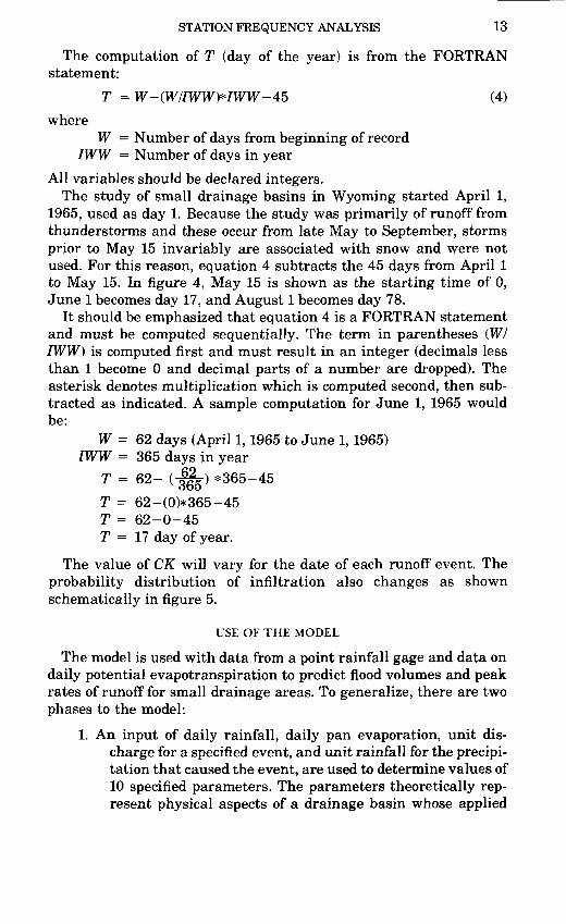
The computation of T (day of the year) is from the FORTRAN statement:
T = W-(W/IWW)*IWW-45 (4)
whereW = Number of days from beginning of record
IWW = Number of days in year
All variables should be declared integers.The study of small drainage basins in Wyoming started April 1,
1965, used as day 1. Because the study was primarily of runoff from thunderstorms and these occur from late May to September, storms prior to May 15 invariably are associated with snow and were not used. For this reason, equation 4 subtracts the 45 days from April 1 to May 15. In figure 4, May 15 is shown as the starting time of 0, June 1 becomes day 17, and August 1 becomes day 78.
It should be emphasized that equation 4 is a FORTRAN statement and must be computed sequentially. The term in parentheses (W/ IWW) is computed first and must result in an integer (decimals less than 1 become 0 and decimal parts of a number are dropped). The asterisk denotes multiplication which is computed second, then sub tracted as indicated. A sample computation for June 1, 1965 would be:
W = 62 days (April 1,1965 to June 1,1965) IWW = 365 days in year
T = 62- (-J^) *365-45
T = 62-(0)* 365-45T = 62-0-45T = 17 day of year.
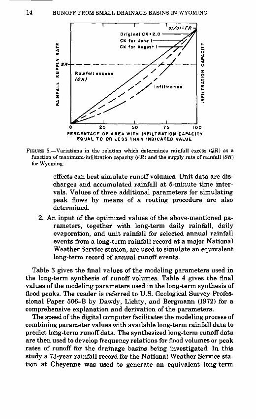
The value of CK will vary for the date of each runoff event. The probability distribution of infiltration also changes as shown schematically in figure 5.
USE OF THE MODEL
The model is used with data from a point rainfall gage and data on daily potential evapotranspiration to predict flood volumes and peak rates of runoff for small drainage areas. To generalize, there are two phases to the model:
1. An input of daily rainfall, daily pan evaporation, unit dis charge for a specified event, and unit rainfall for the precipi tation that caused the event, are used to determine values of 10 specified parameters. The parameters theoretically rep resent physical aspects of a drainage basin whose applied
14 RUNOFF FROM SMALL DRAINAGE BASINS IN WYOMING
Original CK=2.0 CK for June I
0 25 50 75 100PERCENTAGE OF AREA WITH INFILTRATION CAPACITY
EQUAL TO OR LESS THAN INDICATED VALUE
FIGURE 5. Variations in the relation which determines rainfall excess (QR) as a function of maximum-infiltration capacity (FR) and the supply rate of rainfall (SR) for Wyoming.
effects can best simulate runoff volumes. Unit data are dis charges and accumulated rainfall at 5-minute time inter vals. Values of three additional parameters for simulating peak flows by means of a routing procedure are also determined.
2. An input of the optimized values of the above-mentioned pa rameters, together with long-term daily rainfall, daily evaporation, and unit rainfall for selected annual rainfall events from a long-term rainfall record at a major National Weather Service station, are used to simulate an equivalent long-term record of annual runoff events.
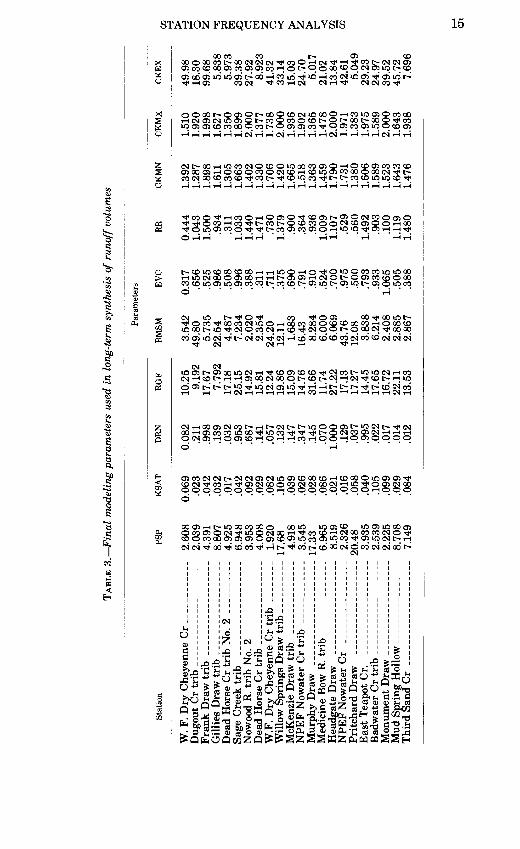
Table 3 gives the final values of the modeling parameters used in the long-term synthesis of runoff volumes. Table 4 gives the final values of the modeling parameters used in the long-term synthesis of flood peaks. The reader is referred to U.S. Geological Survey Profes sional Paper 506-B by Dawdy, Lichty, and Bergmann (1972) for a comprehensive explanation and derivation of the parameters.
The speed of the digital computer facilitates the modeling process of combining parameter values with available long-term rainfall data to predict long-term runoff data. The synthesized long-term runoff data are then used to develop frequency relations for flood volumes or peak rates of runoff for the drainage basins being investigated. In this study a 73-year rainfall record for the National Weather Service sta tion at Cheyenne was used to generate an equivalent long-term
STATION FREQUENCY ANALYSIS 15
OOCO CO O5 CO
CO (N * CO ,-H (N (N t-H
OOOOl>OO5Ol>OOOCO<NmoOO,-ICOinO5OcOOO
<Nl>00,-|lOCO<NOCOOinoOCOO5Oi-lOCOO5COCOCO
CO Tj< O <35 OOTjtOOlOO I 00 CO 00 OCD CD 00 CO r-jO 00 CD- ------ ~> oo c<i-^ QO oo
(N
(N <N
lOOOOOOOOi-HOOO
00 O5 i-H l> IO 00 CO 00 O 00 «2 1C O5 CO IO O5 IO 00 O5
ci ci * od Tj< co co *' i-i i> * co t> co' °o ci o co' (N ci oo' t>^H ^H (N
« x^ ^v ja x ̂ 3 AI'g'S'-Sfi'c-0 £*&£«£^2|g««
X'Cx$-
^H *
° &
v cc
§£>>£
X
£**i-l *;
& >Hn rrl Ol
*J H h^^'B^/s! ^ H ^ ^C oi^ S a>*2
^ofa.M
16 RUNOFF FROM SMALL DRAINAGE BASINS IN WYOMING
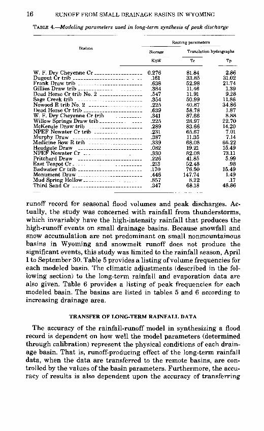
TABLE 4. Modeling parameters used in long-term synthesis of peak discharge
Station
W. F. Dry Cheyenne Cr
Frank Draw trib
Dead Horse Cr trib No. 2Sage Creek tribNowood R trib No. 2
W. F. Dry Cheyenne Cr tribWillow Springs Draw tribMcKenzie Draw tribNPEF Nowater Cr tribMurphy DrawMedicine Bow R tribHeadgate DrawNPEF Nowater CrPritchard DrawEast Teapot CrBadwater Cr tribMonument Draw
Third Sand Cr _ _____ _ _ _ __
Storage
KSW
__ _ 0.276______ .161
__ _ .638_ __ .384___ _ .547______ .354______ .225______ .639_ __ .341_____ _ .225______ .289
.231______ .387______ .339______ .082______ .330______ .226___ .213___ .170_____ .446___ _ .857___ .347
Routing parameters
Translation hydrographs
Tc
81.8433.85 52.98 11.46 11.91 50.99 40.87 58.78 87.66 28.97 83.66 65.67 11.35 68.08 19.21 82.08 41.85 52.48 76.50
147.74 8.22
68.18
Tp
2.86 31.02 21.74
1.39 9.28
11.86 34.86
1.87 8.88
22.70 14.20
7.01 7.14
66.22 15.49 73.11 5.99
.98 15.49
1.49 .17
48.86
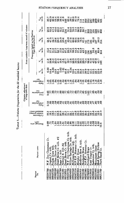
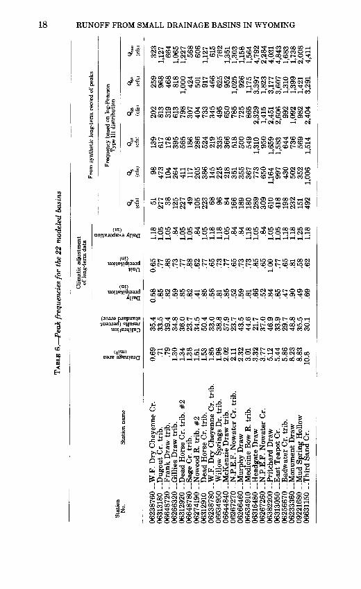
runoff record for seasonal flood volumes and peak discharges. Ac tually, the study was concerned with rainfall from thunderstorms, which invariably have the high-intensity rainfall that produces the high-runoff events on small drainage basins. Because snowfall and snow accumulation are not predominant on small nonmountainous basins in Wyoming and snowmelt runoff does not produce the significant events, this study was limited to the rainfall season, April 1 to September 30. Table 5 provides a listing of volume frequencies for each modeled basin. The climatic adjustments (described in the fol lowing section) to the long-term rainfall and evaporation data are also given. Table 6 provides a listing of peak frequencies for each modeled basin. The basins are listed in tables 5 and 6 according to increasing drainage area.
TRANSFER OF LONG-TERM RAINFALL DATA
The accuracy of the rainfall-runoff model in synthesizing a flood record is dependent on how well the model parameters (determined through calibration) represent the physical conditions of each drain age basin. That is, runoff-producing effect of the long-term rainfall data, when the data are transferred to the remote basins, are con trolled by the values of the basin parameters. Furthermore, the accu racy of results is also dependent upon the accuracy of transferring
STATION FREQUENCY ANALYSIS 17
-a
«.
£i)g3
2
.
1 tf 1 b£-2 *3 -2 &S g'C §
<Neoco<Neoco<Neo(Ncoco<N<Ncoeo<Neoeo<N(N<Nco cocococococococococococococococococococoosco oooooooooooooooooooooo
18 RUNOFF FROM SMALL DRAINAGE BASINS IN WYOMING
s
s
(JOU3
rH r- I r-H rH rH <N ^
lOCOCDt-IO<NO.-ICO<Nin<N<N|>Ci<Nl>Ot-iai<NCit-eo oo
i T i i eo t-fco tti i t-i" t-Teo
rHOOOOOOOOOrHrHOOOaOrHOOOOOrHr-HCNrH
OSr-lOSO'<tOOr-ieOkOOO(Nr-l(Nr-l(NI>(N'<ttO CO'COtpO
o<uc c
(N* jg
X2 c
c oW _Q ju *-" ^-iJt-ii iju ^ ^;^a-c-s^ js^-^ai-s. w &-s& r *̂j
._. _ J(NCOC«3(N<N(NCD _> CO CO CO CO CO CD CD CD O5 CO
ooooooooooooo
STATION FREQUENCY ANALYSIS 19
long-term rainfall data, made difficult by a lack of National Weather Service stations with long records in locations near the study sites.
Because Wyoming has many mountain ranges and large plains, it cannot be expected that identical rainfall patterns will occur at all sites in the State. Also, the long-term National Weather Service sta tion for rainfall data, located in Cheyenne in the southeast corner of the State, cannot be considered as ideally situated to represent the entire State. However, the Cheyenne station does have the longest available record, 73 years, and it can be related to the other Weather Service stations in the State.
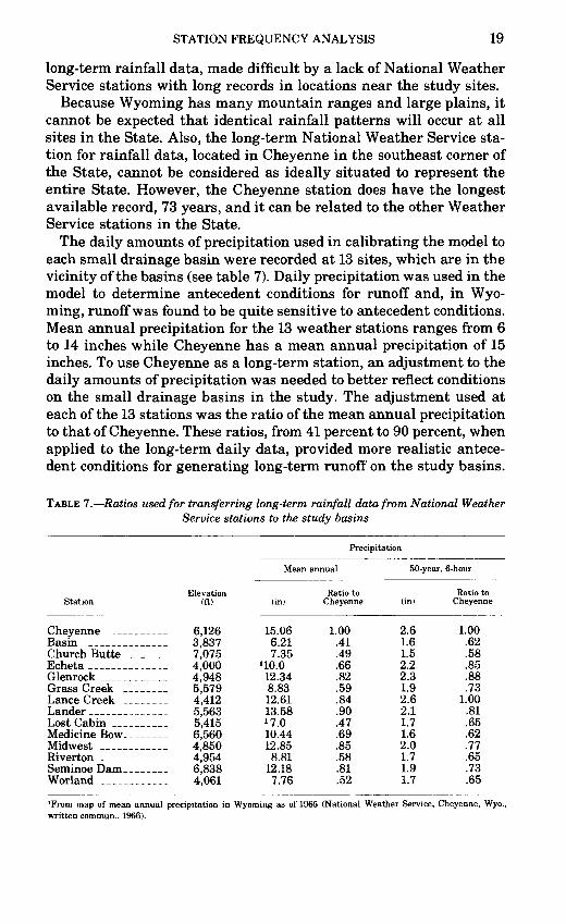
The daily amounts of precipitation used in calibrating the model to each small drainage basin were recorded at 13 sites, which are in the vicinity of the basins (see table 7). Daily precipitation was used in the model to determine antecedent conditions for runoff and, in Wyo ming, runoff was found to be quite sensitive to antecedent conditions. Mean annual precipitation for the 13 weather stations ranges from 6 to 14 inches while Cheyenne has a mean annual precipitation of 15 inches. To use Cheyenne as a long-term station, an adjustment to the daily amounts of precipitation was needed to better reflect conditions on the small drainage basins in the study. The adjustment used at each of the 13 stations was the ratio of the mean annual precipitation to that of Cheyenne. These ratios, from 41 percent to 90 percent, when applied to the long-term daily data, provided more realistic antece dent conditions for generating long-term runoff on the study basins.
TABLE 7. Ratios used for transferring long-term rainfall data from National Weather Service stations to the study basins
Precipitation
Mean annual
Station
Cheyenne
Church Butte _Echeta _ __GlenrockGrass CreekLance CreekLanderLost Cabin .Medicine Bow_Midwest _ _Riverton _Seminoe Dam _
Elevation(ft)
6,126.___ 3,837._._ 7,075
4,000.... 4,948
5,579.___ 4,412
5,5635,4156,5604,8504,9546,8384,061
(in)
15.06 6.21 7.35
UO.O 12.34 8.83 12.61 13.58 J 7.0 10.44 12.85
8.81 12.18 7.76
Ratio to Cheyenne
1.00 .41 .49 .66 .82 .59 .84 .90 .47 .69 .85 .58 .81 .52
50-year, 6-hour
(in)
2.6 1.6 1.5 2.2 2.3 1.9 2.6 2.1 1.7 1.6 2.0 1.7 1.9 1.7
Ratio to Cheyenne
1.00 .62 .58 .85 .88 .73
1.00 .81 .65 .62 .77 .65 .73 .65
'From map of mean annual precipitation in Wyoming as of 1965 (National Weather Service, Cheyenne, Wyo., written commun., 1966).
20 RUNOFF FROM SMALL DRAINAGE BASINS IN WYOMING
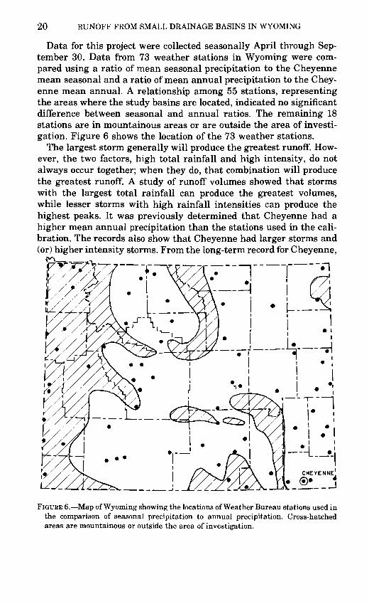
Data for this project were collected seasonally April through Sep tember 30. Data from 73 weather stations in Wyoming were com pared using a ratio of mean seasonal precipitation to the Cheyenne mean seasonal and a ratio of mean annual precipitation to the Chey enne mean annual. A relationship among 55 stations, representing the areas where the study basins are located, indicated no significant difference between seasonal and annual ratios. The remaining 18 stations are in mountainous areas or are outside the area of investi gation. Figure 6 shows the location of the 73 weather stations.
The largest storm generally will produce the greatest runoff. How ever, the two factors, high total rainfall and high intensity, do not always occur together; when they do, that combination will produce the greatest runoff. A study of runoff volumes showed that storms with the largest total rainfall can produce the greatest volumes, while lesser storms with high rainfall intensities can produce the highest peaks. It was previously determined that Cheyenne had a higher mean annual precipitation than the stations used in the cali bration. The records also show that Cheyenne had larger storms and (or) higher intensity storms. From the long-term record for Cheyenne,
^~T2
FIGURE 6. Map of Wyoming showing the locations of Weather Bureau stations used in the comparison of seasonal precipitation to annual precipitation. Cross-hatched areas are mountainous or outside the area of investigation.
STATION FREQUENCY ANALYSIS 21
the largest storms for each year were selected as potentially capable of producing the annual peak runoff. When a single storm had un questionably produced the annual maximum rainfall, only that one storm was used. Generally, two or three storms were chosen. The same rainfall data are used in the rainfall-runoff model to generate either long-term annual peaks or long-term annual runoff volumes. When two or more storms in the same year are used, it is not unusual for one storm to produce the annual peak while a different storm produces the annual volume.
In order to transfer rainfall recorded at Cheyenne to each remote drainage basin for generating runoff, an adjustment was considered necessary. Rather than use the ratios of the mean annual precipita tion, as was done for daily values of rainfall totals, an adjustment was needed that would have a lesser effect on rainfall intensity. From the 73-year precipitation record for Cheyenne, 133 storms were used to simulate runoff. The average duration per storm was 4.7 hours. An analysis was made of depth-duration frequency maps of Wyoming (National Oceanic and Atmospheric Admin., 1974) for 6-hour and 24-hour durations and 2-, 5-, 10-, 25-, and 100-year recurrence inter vals. By interpolation, the 50-year, 6-hour frequency duration was selected as most applicable. The ratio of the 50-year, 6-hour occur rence at each weather station to that at the Cheyenne weather sta tion provided the adjustment factor. Values for the 50-year, 6-hour frequency duration at each station and for the ratio to Cheyenne are given in table 7. For 9 of the 13 stations, this ratio was higher than the ratio of the mean annual precipitation and, when applied, would have a lesser effect on the intensities than would the ratio of the mean annual precipitation. Intensities for the remaining four sta tions would be reduced by using this ratio, but these are stations with comparatively high ratios of mean annual precipitation, so the reduc tions are not great.
TRANSFER OF LONG-TERM EVAPORATION DATA
Only seven weather stations in Wyoming have evaporation data for 20 years or more and only 12 stations have any evaporation data. The longest evaporation record available (60 years through 1973) is for Archer, located about 9 miles east of the Cheyenne weather station. The proximity of this station to Cheyenne and the length of record made it ideal for use in the long-term runoff simulation phase of the rainfall-runoff model. However, because the same period and length of record are needed for precipitation and evaporation, the evapora tion record for Archer had to be extended backward from 1913 to 1901. This extension was made by developing a correlation between
22 RUNOFF FROM SMALL DRAINAGE BASINS IN WYOMING
6-month periods of evaporation and 6-month periods of precipitation, for 15 years of selected record as shown in figure 7. Certain years were selected to increase the range of the comparison. Two years of exces sive precipitation with high evaporation were considered nonrep- resentative and were not used. The equation determined from a corre lation of 13 years of record was
y = 49.40 - 1.217 xwhere:
x = seasonal precipitation y = seasonal evaporation
with a correlation coefficient of 0.93 and a standard error of 13 percent.
The same 13 years were used to compute the average evaporation for each day. The daily values were adjusted by a ratio of the com puted evaporation from the equation and the mean evaporation for the 13 years. This procedure resulted in reduced evaporation values for seasons of above-normal precipitation and increased evaporation values for seasons of below-normal precipitation.
The evaporation data for Archer were not used in the initial cali bration of the study basins. Instead, four stations closer to the basins were used (table 8).
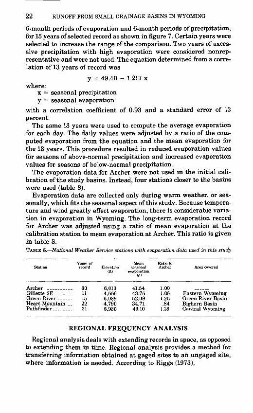
Evaporation data are collected only during warm weather, or sea sonally, which fits the seasonal aspect of this study. Because tempera ture and wind greatly effect evaporation, there is considerable varia tion in evaporation in Wyoming. The long-term evaporation record for Archer was adjusted using a ratio of mean evaporation at the calibration station to mean evaporation at Archer. This ratio is given in table 8.TABLE 8. National Weather Service stations with evaporation data used in this study
Station
ArcherGillette 2EGreen RiverHeart Mountain _ Pathfinder
Years of record
60111522 31
Elevation(ft)
6,0104,5566,0894,790 5,930
Mean seasonal
evaporation(in)
41.5443.7552.0934.71 49.10
Ratio to Archer
1.001.051.25.84
1.18
Area covered
Eastern Wyoming
Bighorn Basin
REGIONAL FREQUENCY ANALYSIS
Regional analysis deals with extending records in space, as opposed to extending them in time. Regional analysis provides a method for transferring information obtained at gaged sites to an ungaged site, where information is needed. According to Riggs (1973),
REGIONAL FREQUENCY ANALYSIS 23
O
o
O
o
o
o
(A) S3HONI Nl 'dOIH3d H1NOW-XIS 'NOIlVdOdVA3 1VNOSV3S
<£. ~ H
* I §co g'-g
in LU £ "«
O T3 g
.3 X «
Q O
- cc.LU CL
CM i_O 0)
'J3 Vi
II
a 8, S
* ^ I §0 £ aS II
00 Q_ * .*J
2 g fto § aCO « «
LU CO
24 RUNOFF FROM SMALL DRAINAGE BASINS IN WYOMING
multiple regression is directly useful as a regionalization tool because the discharge (or volume) can be related to basin characteristics, leaving residuals that may be considered as due to chance. The regression line averages these residuals. Thus, in one operation, the effects of differing basin characteristics are preserved and the chance variation is averaged.
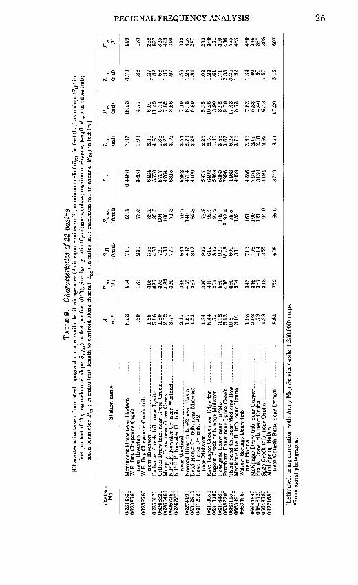
BASIN CHARACTERISTICS
Basin characteristics, used as independent parameters in the re gression analyses, are summarized in table 9 and are defined below. Areas were planimetered from the best available topographic maps. Measurements of length along channel, basin perimeter, or contour lines were obtained by stepping with draftsman's dividers set at a scale interval of 200 feet.
A Drainage area, in square miles.Rm Maximum relief in basin, in feet; the difference in eleva
tion between the channel at the gage and the highest point in the basin, determined from topographic maps.
SB Basin slope, in feet per mile, obtained by measuring the lengths (in miles) of all contour lines within the drain age boundary, multiplying by the contour interval in feet, and dividing by the drainage area in square miles. Reasonable accuracy can be obtained on most topo graphic maps by measuring only the 100-foot contour lines.
<S10/85 Main-channel slope, in feet per mile, determined from elevations at points 10 and 85 percent of the distance along the channel from the gaging station to drainage- basin divide.
Lm Main channel length, in miles, from the gaging station tothe drainage-basin divide.
Cr Circularity ratio, dimensionless; the ratio of basin area to the area of a circle having the same perimeter as the basin.
Pm Basin perimeter, in miles; the length of the drainage area boundary.
Lca A measured length in miles along the main-stem channel from the gaging station to the point opposite the cen- troid of the total drainage area (Chow, 1964).
Fm Maximum fall in channel, in feet; the total difference in elevation between the channel bottom at the gage and the point where the extended main channel reaches the drainage boundary.
The basin characteristics defined above were used in regression analyses to develop relations for estimating peak discharge or runoff volume.
TABL
E 9
. C
hara
cter
isti
cs o
f 22
basi
ns[C
hara
cter
istic
s ta
ken
from
lat
est
topo
grap
hic
map
s av
aila
ble.
Dra
inag
e ar
ea 0
4) i
n sq
uare
mile
s (m
i2);
max
imum
rel
ief (
Rm
) in
feet
(ft)
; bas
in s
lope
(Sg
) in
fe
et p
er f
eet
(ft/f
t); m
ain-
chan
nel
slop
e (S
JO/8
5) i
n fe
et p
er f
eet
(ft/f
t); c
ircu
lari
ty r
atio
(Cr
) dim
ensi
onle
ss;
max
imum
cha
nnel
len
gth
(Lm
) in
mile
s (m
i);
basi
n pe
rim
eter
(Pm
); i
n m
iles
(mi);
len
gth
to c
entr
oid
alon
g ch
anne
l (L
ca) i
n m
iles
(mi);
max
imum
fal
l in
cha
nnel
(Fm
) in
feet
(ft)
]
Stat
ion
No.
Sta
tion
nam
eA
(m
i2)
(ft)
SB (ft/m
i)(f
t/mi)
(mi)
(mi)
(mi)
(ft)
0623
3360
M
onum
ent
Dra
w n
ear
Hud
son
__
. 06
2387
60
W.F
. D
ry C
heye
nne
Cre
ekne
ar R
iver
ton
-___
____
__-_
- __
_-06
2387
80
W.F
. D
ry C
heye
nne
Cre
ek t
rib.
near
Riv
erto
n -_
____
____
----
____
.06
2566
70
Bad
wat
er C
reek
tri
b. n
ear
Lys
ite .
..
0626
6320
G
illie
s D
raw
tri
b. n
ear
Gra
ss C
reek
. 06
2664
60
Mur
phy
Dra
w n
ear
Gra
ss C
reek
__
. 06
2672
60
N.P
.E.F
. N
owat
er C
r. ne
ar W
orla
nd.
0626
7270
N
.P.E
.F.
Now
ater
Cr.
trib
.ne
ar W
orla
nd ______._
___.
0627
4190
N
owoo
d R
iver
tri
b. #
2 ne
ar B
asin
__.
0631
2910
D
ead
Hor
se C
r. tr
ib.
near
Mid
wes
t .
0631
2920
D
ead
Hor
se C
r. tr
ib.
#2ne
ar M
idw
est
____
____
____
____
_06
3130
50
Eas
t T
eapo
t C
reek
nea
r E
dger
ton
__.
0631
3180
D
ugou
t C
reek
tri
b. n
ear
Mid
wes
t __
. 06
3164
80
Hea
dgat
e D
raw
nea
r B
uffa
lo _
__-
0638
2200
P
ritc
hard
Dra
w n
ear
Lan
ce C
reek
._.
0663
1150
T
hird
San
d C
r. ne
ar M
edic
ine
Bow
.
0663
4910
M
edic
ine
Bow
R.
trib
. ne
ar H
anna
.
0663
4950
W
illow
Spr
ings
Dra
w t
rib.
near
Han
na -
_____
0664
4840
M
cKen
zie
Dra
w t
rib.
nea
r C
aspe
r .
0664
8720
F
rank
Dra
w t
rib.
nea
r O
rpha
..._.
0664
8780
Sa
ge C
reek
tri
b. n
ear
Orp
ha
____.
0922
1680
M
ud S
prin
g H
ollo
wne
ar C
hurc
h B
utte
nea
r L
yman
__.
8.23
.69
1.85
5.86
1.30
2.32
3.77
2.11
1.51
1.53
1.34
5.44 .7
13.
325.
1210
.8 3.01
1.98
2.02 .7
91.
38
8.83
594
173
316
627
375
4.83 320
338
405
287
320
430
201
550
436
680
504
543
346
337
318
752
719
240
356
483
720
431
771
63
44
37
847
922
612
831
929
'618
60
9 55
0
719
498
414
355
60
8
59.1
76.6
88.2
85.5
204
106 71
.3
79.7
140 62.3
73.9
92.9
97.2
102
2 92
.475
.513
2
161
100
121 94
.0
66.5
0.44
58
.389
8
.642
4.5
570
.572
7.4
764
.631
5
.526
2.4
734
.440
9
.587
7.6
492
.586
8.5
363
.799
6.4
463
.495
9
.428
6.7
454
.513
0.4
194
.374
9
7.97
1.93
2.39
4.85
1.35
3.20
3.05
3.54
2.73
3.28
2.25
2.69
1.40
3.55
3.67
6.27
3.79
2.39
2.19
2.01
2.92
8.11
15.2
3
4.71
6.01
11.4
95.
347.
828.
66
7.10
6.33
6.60
5.35
10.2
63.
908.
829.
3017
.43
8.73
7.62
5.83
4.40
6.43
17.2
0
3.79
1.27
1.82 .6
81.
35 .97
1.59
1.25
1.84
1.02
1.24 .6
11.
712.
533.
251.
92
1.34
1.02 .9
01.
50
5.12
519
173
258
627
325
423
310
322
405
287
233
380
171
390
436
575
483
430
34
633
73
08
607
Q
O O cc
'Est
imat
ed,
usin
g co
rrel
atio
n w
ith A
rmy
Map
Ser
vice
(sc
ale:
1:2
50,0
00)
map
s.
2Fro
m a
eria
l ph
otog
raph
s.
bO 01
26 RUNOFF FROM SMALL DRAINAGE BASINS IN WYOMING
REGRESSION ANALYSIS
The purpose of regionalization is to define relations that can be used to estimate runoff at ungaged sites. In this study a rainfall- runoff model was used to produce a synthetic long-term runoff record from an actual long-term rainfall record. The synthesized peaks and volumes were used in the development of station frequency curves. From these curves, specific frequencies were selected for regression analysis of basin characteristics in a regional study. Because only one long-term rainfall record (Cheyenne) was used, the results of this regional analysis appear better than they might otherwise be. Chey enne was selected as the base rain gage because it had the longest record and because it had the open exposure (less influenced by nearby orographic effects) to provide a better analogy to the study basins. The adjustments described in the preceding section in transferring the rainfall data to other weather stations in Wyoming were primarily to reduce the amounts and intensity of Cheyenne rainfall data. The transferred data at some weather stations were used to develop long-term runoff records at two or more gaged sites, resulting in interdependency of synthesized flood occurrences among these sites. Because of this interstation correlation, discussed by Matalas and Benson (1961), the slope of a regional relation is better defined than that of a relation obtained from a purely random sample, but its position (intercept) is less well defined.
The regression model used in regional frequency analysis is of the form,
Qn or Vn = aA b>B b* O *****,
the log transform of which is linear. Peak discharges and runoff vol umes with recurrence intervals of 2, 5, 10, 25, 50, and 100 years for 22 small basins were selected for analysis. Independent variables were chosen on the basis of logical physical relationship to streamflow for small drainage basins and tested for significance using a "step- forward" regression program. The basin characteristics were used in regression analyses to develop relations for estimating peak dis charges or runoff volumes. (See the section on "Basin Characteris tics.") The basin characteristics determined to be most significant in estimating peak discharge were drainage area, basin slope, maximum basin relief, and main-channel slope. The correlation coef ficients ranged from 0.89 to 0.92 and the standard errors of estimate from 32 to 38 percent.
Estimates of peak discharge are mainly dependent on drainage area and basin slope, with correlation coefficients of 0.81 to 0.88 and standard errors of 37 to 48 percent, respectively. The addition of maximum basin relief and channel slope, in that order, improved the
REGIONAL FREQUENCY ANALYSIS 27
correlation and reduced the standard error by small amounts of from 1 to 6 percent. The designer would have to decide whether the in crease in correlation and reduction in standard error warranted the inclusion of the variables in the equation.
Drainage area, maximum basin relief, and basin slope proved to be the most significant parameters for estimating runoff volume. The correlation coefficients ranged from 0.92 to 0.93 and the standard errors of estimate from 30 to 32 percent.
In an analysis of residuals the residual variations indicated an areal randomness and were probably due to chance variation or some untested basin characteristics. Geographical subregions were not ap parent in this study.
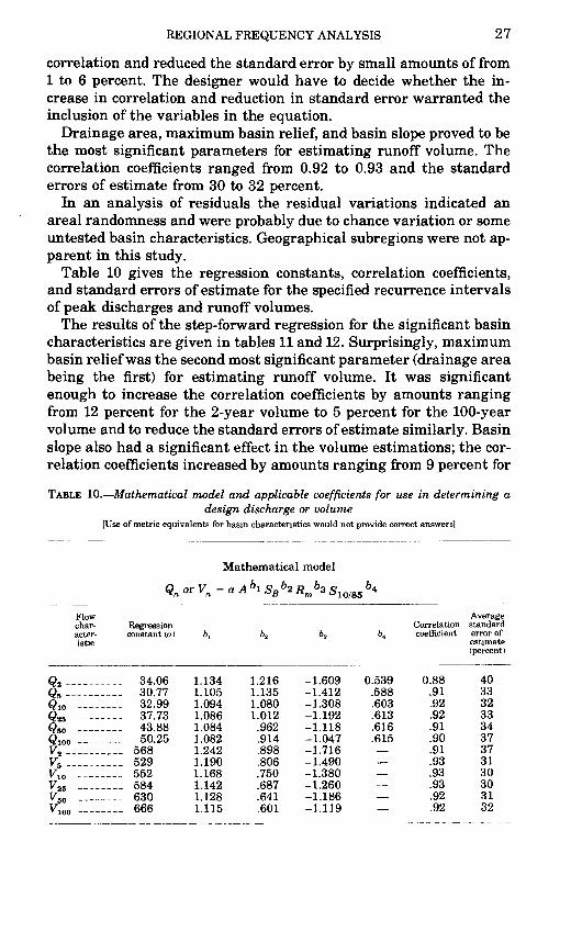
Table 10 gives the regression constants, correlation coefficients, and standard errors of estimate for the specified recurrence intervals of peak discharges and runoff volumes.
The results of the step-forward regression for the significant basin characteristics are given in tables 11 and 12. Surprisingly, maximum basin relief was the second most significant parameter (drainage area being the first) for estimating runoff volume. It was significant enough to increase the correlation coefficients by amounts ranging from 12 percent for the 2-year volume to 5 percent for the 100-year volume and to reduce the standard errors of estimate similarly. Basin slope also had a significant effect in the volume estimations; the cor relation coefficients increased by amounts ranging from 9 percent for
TABLE 10. Mathematical model and applicable coefficients for use in determining a design discharge or volume
[Use of metric equivalents for basin characteristics would not provide correct answers]
Mathematical model
Flow char acter istic
QQ2Q*Q10
Q50 __ .
yzy5
V25 ____.
y50
Regression constant (a )
.___ 34.06
.___ 30.77
..__ 32.99 _ 37.73.___ 43.88-_ _ 50.25-- 568..__ 529.___ 552. _ 584 _ 630. _ 666
*,
1.1341.1051.0941.0861.0841.0821.2421.1901.1681.1421.1281.115
,
1.2161.1351.0801.012.962.914.898.806.750.687.641.601
,
-1.609-1.412-1.308-1.192-1.118-1.047-1.716-1.490-1.380-1.260-1.186
1.119
.
0.539.588.603.613.616.615
_____
Correlation coefficient
0.88.91.92.92.91.90.91.93.93.93.92.92
Average standard error of estimate (percent)
403332333437373130303132
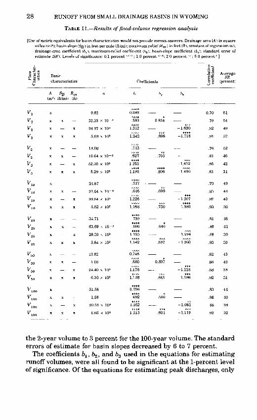
28 RUNOFF FROM SMALL DRAINAGE BASINS IN WYOMING
TABLE 11. Results of flood-volume regression analysis
[Use of metric equivalents for basin characteristics would not provide correct answers. Drainage area (A ) in square miles (mi2 ); basin slope (Sg ) in feet per mile (ft/mi); maximum relief (Rm ) in feet (ft); constant of regression (a); drainage-area coefficient (bl ); maximum-relief coefficient (62 ); basin-slope coefficient (63 1; standard error of estimate (SE). Levels of significance: 0.1 percent ****; 1.0 percent ***; 2.0 percent **; 5.0 percent *]
Flow Character
istics
v,^2
V2
V2
V5
V5
V5
v*vlo^10
vloV10
V25V25
V25
V25
V50
V50
V50
V50
*100
100^100
' 1 AA
Basic characteristics
A SB Rm(m2 ! (ft/mi) (ft)
x
XX
X X
XXX
X
XX
X X
XXX
X
XX
X X
XXX
X
XX
X X
XXX
X
XX
X X
XXX
X
XX
X X
XXX
Coefficients
Correlation coefficient
Average SE
(percent)
a b1 62 63
9.62
52.53 x
94.97 x
5.68 x
18.08
16.64 x
52.30 x
5.29 x
24.87
31.54 x
39.84 x
5.52 x
34.71
63.69 x
29.30 x
5.84 x
42.82
1.03
24.40 x
6.30 x
51.58
1.56
20.53 x
6.66 x
io-3103
IO2
io- 2IO3
IO2
io- 2IO3
IO2
io- 2IO3
IO2
IO3
IO2
IO3
IO2
0*6*89
****.593
1*312
1.242
.713
.627
1.253
1*190
.727####
.646
1.226
1.168
.739
.6661*1*95
1.142
0*748*680
1.178****
1.128
0*756
*692
1*162
1.115
0.834
.898
.705
*806
. __*#
.699
.750
.640
.687
__
0.597
.641
.560
.601
-1.630
-1*716
-1.412
-1.490
__
-1.307
-1*380
-1.194-1*2*60
__
-1.124
-1.186
-1.061
-1.119
0.70
.79
.82
.91
.76
.83
.86
.93
.79
.85
.87
.93
.81
.86
.88
.93
.82
.86
.88
.92
.83
.86
.88
.92
61
54
49
37
52
46
42
31
49
43
40
30
46
41
39
30
45
40
38
31
44
40
38
32
the 2-year volume to 3 percent for the 100-year volume. The standard errors of estimate for basin slopes decreased by 6 to 7 percent.
The coefficients blt bz , and b3 used in the equations for estimating runoff volumes, were all found to be significant at the 1-percent level of significance. Of the equations for estimating peak discharges, only
A. __ ___SB - r>
A - 1.00
97
.83- .37
SB
1.00.25
- OR
Rm
1 00.03
REGIONAL FREQUENCY ANALYSIS 29
the coefficients hi and bz are significant at the 1-percent level. The coefficients 63 and b4 show a deterioration in the level of significance; 63 ranges from the 1-percent level in estimating Q2 to the 10-percent level in estimating Q100 , and b4 ranges from the 10-percent level in estimating Q5-Q50 to the 20-percent level in estimating Q2 and Q100 .
Among independent variables there is a fairly high correlation between drainage area and maximum basin relief. The other vari ables indicate little cross correlation. The correlation matrix is shown below.
S10/»
1.00
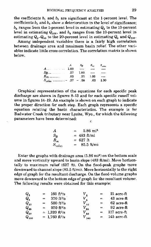
Graphical representation of the equations for each specific peak discharge are shown in figures 8-13 and for each specific runoff vol ume in figures 14-19. An example is shown on each graph to indicate the proper direction for each step. Each graph represents a specific equation relating the basin characteristics. The example is for Badwater Creek tributary near Lysite, Wyo., for which the following parameters have been determined:
A = 5.86 mi2SB = 483 ft/miRm = 627 ftS10/85 = 85.5 ft/mi
Enter the graphs with drainage area (5.86 mi2 ) on the bottom scale and move vertically upward to basin slope (483 ft/mi). Move horizon tally to maximum relief (627 ft). On the flood-peak graphs move downward to channel slope (85.5 ft/mi). Move horizontally to the right edge of graph for the resultant discharge. On the flood-volume graphs move downward to the bottom edge of graph for the resultant volume. The following results were obtained for this example:
Q2 = 160ft3/s V2 = 21acre-ftQ5 = 370 ft3/s' V5 = 43 acre-ftQ 10 = 580 ft3/s V10 = 62 acre-ftQ25 = 950ft3/s V25 = 92 acre-ftQ50 = 1,320 ft3/s V50 = 117 acre-ftQ100 = 1,760 ft3/s V100 = 145 acre-ft
O <O <O <O <O w c« en en en
X X X X X
X J 1^1
X I X j |
i * i i i
i 'tO h-» tO CD^ jo en t » CDoo en to en 05to oo en if^
XXXt ' 1 ' h- '
10 CO |
10
00* O5* CD* i^* O5 * H-»* O* O* 00* H-1 *o* *.* en* 05* to*
r# ^* f-1* i ! b* i10* ' j CD* '05* ! i co* !
1 1
'& ', '~J \ \ -3 O5 i > J* i oo o ! !
1! b ! i ! en i ! en o ! ! i
CD O5 ^J 00 O5 O CD tO O5 CD
co en en * enen -3 i^ o 05
<O <O
* !
X X
X X
CO CO>fik "^
O COO5 H-1
X
ow
i ' I 1I * 10* CO* O*
H-
to* ! H-1*
O5* !
1 1
o* en,CD* OT
col" CDCD+ CO o
00 -J 00 O
^ O5o to
<o 10
X
!1
1x1
I-100toCO
X
o1 10
*.*O5*
rI-1*
o*
i
1to toCO o
00to
t^CD
<o <o <o «o <o 10 10 10 10 10
x i i x i
X ' X ' *
i * i i i
10 10 CD 3 tO ~] _. O5
CD co co en to00 CD CD ^ h->
x x o_ i- X«2 <3 H-
o1
CO
. * - Poo* en* CD* *.* en* <i* en* O5* oo* oo* o* *> * en* oo* to*
!""* !~"to* ! ! H-* i O* ! ! O5* ! Oo* 1 ! O5* !
1 1 |-> H-1
f- ! 0 1 > i O i ioo* ! I-* o ! !
1 p
! CD 1 > i! en o ! ! !
O00 O5 O5 00 ;_<l CO 00 H- g
^ O5 O5 »^ O5
Flowcharacteristics
g~
ft?^;
^3'
s> toIs-
0
*
"*
sr
|w3.3'
8
o0n 3S' asr
Correlation coefficient
AverageS£
in! r^ w * ' p.° * 8 3
(S S »
Jals- 3 g ?sg. a 3 §
"' g. g 3 § ~ S' §5- Sg s iTS 3 s- ^i r » B. e-f- TO C^ »w < 5 - g> 2. § "*
r£"f 5' > (§' » £-2
5' g. g .8 Crs EJs Eo
m S 8 ffi t"i 4 B $ BO CO P r[> *i
I. p | S, 5o2. *~* S- S ^
si i? "sT cI S a- a S?
E. ^ B H o O- # S' fD ****i
|-j|ff
II" SI"8 1 | 3 ap<
a-j|§| § bp s1 5lip-
3 S 5 3 3" Z. s *Z. o
3 B §-* 3 Is 8.
1 § "a *g 3 »
3- sr
'S -^ <L
§ i- j?385' 2 "> -^& 3 |
+ 11V S 3to * c;O i-r n>
H- 05 H- oo rfs. (percent)
ONIPMOAM NI SNISV9 aOVNIVHQ llVPVtS PVtOHJoe
REGIONAL FREQUENCY ANALYSIS 31
CO COt-<N-'fTfOO<N<N OI>O<N»OOOOCO CO lOCOlOlOCOCOlOCO lOCOlOlOCOCOlOCO
<N O l> CO <N u300COUt>OOOOO<N D~ O} 00 D~ O3 t~OOD~£~O500D~O}
1 1 i ° TJ< 400 ! ! ! ° oo j ° t~ ° T I -LCO ! ! | ° <N | ° oo00 -^ 00 j \ ' O I rH CO O i ! ! t~ ! 3?O IQ IQ ! ! loiomco ! ! !o!o
!*Oi !°CD*00 ! |°l> ! 4-^f ! ° Oi * (N' IO i CD *O ' ' CO ' CO ' IO * Oi! C~ ! rH *CO ! ! U3 ! to i O rH
II I I I I I I I I
! *ooI jn. *
*-* *<N *U3 *<N #<N *CO *-* *Oi *O *00 * -f *O *t> * U3 *O * CO * <* * CO * CD*t- *t> *O * CO *i-H *00 *CO *Oi *rH *U3 *Oi * (O * * *CD * C~ * 00 * 1C * *& * 00*^(» *^H *^H *CD *U3 *00 *CD *C- *U3 *rH *0 * SO **£> * 00 * tO *t> *10 *^H *0
n I n M In I M M InN O OOO OO OOO OO
rnX XXX XX XXX XX
(NU3C-; OOCDOOOO-^OtNOi rHOOrHrHrH-rl»oqi>;
x : x x x iiixixxx
X;XjXX j j X j M ; M M
XXX XXXX
XXX XXXXXXXX XX-XXXXXX
oo o
X
X
X
X
cnotocn
i 10*oo* bO*
co*
1
b
ori-
coo
co^3
^
§
X
1
X
X
COoO5 I "
Xt 'o
I "t-1* co*O5*
i
icobO -J o
cnooO o
CO
cn o
Oo o
X
X
i
X
I "O5
bO
Xt 'o
1»
O5*
cn*
bo* oo* t^.*
,1
i "bOO o
oo
£
.0 ,0 ,0 .0 ,0o o o o o o o o o o
X X X X X
X | | X |
x | x i i
! X ! ! ! i iii
bo -Jt^. O5 00 COo co to oo t-11 ' ^3 Cn O5 t 'bo oo o
X XI 1t ' t ' OO O 1
o* -J# bo* cn* as * oo* to* cn* to* co* t-i* o* to* -j * co*
co* ! ! bo* jO* ' ' 00* t^.* ! I as* !
1 1
j^. ' co oo j co | |Oi o i CO o i i
j t ' ! ! !
' |-1 ° ' ' '
oo -j -j oo -j oo ~J ~j ^J ~J
co cn cn t^. cn co to i > o o
o .0 <oo o o
XXX
x i x
x x i
XXX
t 't^ h-"t f~-tco o cnoo co oooo oo x
X(->(-* OO 1
I-" t-"b* I-1* cn* oo * t^.* oo* t^. * i " * cn*
co* ! co*O5* ' CO*bo* ! o*
1 t >I-1 co ! t-> co oo* to o !
as cn b ) 1| ^3 OO Ojl CO o O^ o
co ^j oo t-i tO ^J
co cn co »^ o co
o .0 .0 ,0 .0 cn cn cn cn cnO O O O O
X X X X X
x | I x i
X | X | |
i x i i : iii
(-> cnCO ^3 ^3 ^Jcn co co t-1 cno »^ ^j co »^* -^ ^ v
x x xt ' (-'(-' OO O 1
K>
o<]* as* bo* cn* as* oo* co* cn* <]* <J # co* cn* -j * to* co*
co* ! ; co* ! cn * i i co* i bo* ! I (-** !
1 1
014- ! £t ' '^LL i o* i ! oar ! as o ! !
i S i i i1 oo o ! ! i
oo <] <] oo <] co o^ ^j ^j o^
co cn cn co cn~3 bO O 00 O
Flowcharacteristics
!>
I*
? 3
?K J*
Si
Q
-»
jr
0-
3*
fb . S'3'
5ttt
t
) fi0:?0^
cc
nC3
(Jcec
ccq&̂«&
r o £ o "- 0) r
3 E
1 s
Correi anon coefficient
AverageSE
(percent)
ONIHOAAV NI SNISV9 3OVNIVHQ 11VHS HOHd ddONnH
REGIONAL FREQUENCY ANALYSIS 33
QN003S 83d 133J OISHO Nl '39yVHOSIQ
,bo o C ""
CO
100
<£
I 10
D
RA
INA
GE
A
RE
A,
IN
SQ
UA
RE
M
ILE
S
10
<0
FIG
URE
9.
Rel
atio
n o
f 5-
year
flo
od p
eak
to d
rain
age
area
, ba
sin
slop
e, m
axim
um r
elie
f, a
ndch
anne
l sl
ope.
§ £ CO O
H
dd
> CO 3 CO 5 H< o g 3 o
REGIONAL FREQUENCY ANALYSIS 35
ON033S M3d 133J 318113 Nl '39aVH3Sld a
cfl
III I I I I I III I I I I I I III I I I I I I III I I I I I I
a 1 &
] I
I I
I I
LCO
O
i
10,0
00
I 10
D
RA
INA
GE
A
RE
A,
IN
SQ
UA
RE
M
ILE
S
10
00
<-> EC < I O
100
W
FIGU
RE 1
1. R
elat
ion
of 2
5-ye
ar f
lood
pea
k to
dra
inag
e ar
ea,
basi
n sl
ope,
max
imum
rel
ief,
and
chan
nel
slop
e.
cc S
> r
o Q
W dd
>
cc
i i
2
cc 3 3 *!
O s § Q
REGIONAL FREQUENCY ANALYSIS 37
QN003S H3d 133J Nl '39dVH3SIQ
\T\ I I T\
0)130 o,
nS
-2 G
CD
< £
I I I I I I 1111 I 1 I I 11111
DISCHARGE, IN CUBIC FEET PER SECOND
ONIWOAM NI SNISVa 3OVNIVHQ 11VWS KEOHd jMONHH
REGIONAL FREQUENCY ANALYSIS 39
I I I I I I I I I I T
UJ
iUJ DC O
o_
UJoc
UJ
oc- Qo
aa
2 £
5 ^*
"- a< .5ID "*"O "S
I I
I I
II It.
O.I
1 J_
I
1 I
1111
i i
r«r
*
"a or
^
^
i M
il i
i i
i i 1
111
i i
i i
111
iJ_
__
i i
i i
i 111
10 i10
10
0 V
OL
UM
E,
IN A
CR
E-F
EE
T10
00D
RA
INA
GE
A
RE
A,
IN
SQ
UA
RE
M
ILE
S
FIG
URE
15. R
elat
ion o
f 5-
year
flo
od v
olum
e to
dra
inag
e ar
ea,
basi
n sl
ope,
and
max
imum
rel
ief.
REGIONAL FREQUENCY ANALYSIS 41
I I I I I I I
I I°xaSa
T3 cd to°LU -a
LU -S
LU
LU
00
LUo:
LU
cr- o o
± ea
42 RUNOFF FROM SMALL DRAINAGE BASINS IN WYOMING
I II I I I
II I I I I I I III I I I I I I III I I I I I I
Xa 8
73ch- «
UJ $uj Jlii *3I B
UJ '3* J8 < «I sUJz15 _l O>
00
UJ
<UJo
oa- o o
§ Io ,5
REGIONAL FREQUENCY ANALYSIS 43
ii i i i i i I |Miiiii i -
ii 11 i i i i In i i i i i i In 11 i i i i
o o o
Ul UJu.
IUJ QL O
O >
OOV) UJ_J
Ul QL
oV)
Ul QL
Ul O
cc
e3
X <Ae a
uT So
I3«
3
I
D.I
I 10 10
10
0 10
00D
RA
INA
GE
A
RE
A,
IN
SQ
UA
RE
M
ILE
S
VO
LU
ME
, IN
AC
RE
-FE
ET
FIG
URE
19.
Rel
atio
n of
100
-yea
r flo
od v
olum
e to
dra
inag
e ar
ea,
basi
n sl
ope,
and
max
imum
rel
ief.
RUNOFF FROM SMALL DRAINAGE BASINS IN WYOMING 45
RELATION OF PEAK DISCHARGE TO RUNOFF VOLUME
Estimation of the flood hydrograph requires knowledge of flood- volume and flood-peak magnitudes. Although the values might be estimated from relations defined in the previous section, flood vol umes at some sites in Wyoming possibly can be estimated from more reliable flood-peak information if it is available. Also, it might be possible to estimate a flood peak from a flood volume rather than from basin characteristics. In this section, relations were defined to test those possibilities.
The problem in relating peak discharge to volume lies in the many variations of conditions prior to and during the occurrence of runoff. The degree of saturation of the soil, the timing and intensity of the rainfall, and the direction of the storm in relation to the basin all affect the size of the peak and volume of runoff. In the model calibra tion of the drainage basins, it was assumed that these various condi tions were accounted for if the conditions were present during the period of record used in the model. It should be understood that not all possible conditions can be accounted for on all basins. The effect of modeling is that of averaging conditions and reactions for the basin.
Graphs from rain-recording instruments showing increases or de creases in the rainfall intensities may explain some of the variations in shape of the runoff hydrograph. A runoff hydrograph from a small drainage basin will usually reflect changes in the rainfall pattern, but these variations cannot be anticipated and cannot be incorporated in a design hydrograph. It can be shown that the simple fast-rising hydrograph has the greatest potential for causing problems at cul verts and bridges. (See section on "Embankment Storage.") The com posite MDH (Mean Dimensionless Hydrograph) (discussed in next section of this report) produces such a graph.
Because peak discharge and runoff volume are both essential to the composite MDH, a relation between peak discharge and volume is desirable. A study of runoff hydrographs from 35 drainage basins indicates that such a relation exists. Three hydrographs from each basin were selected on the basis of shape, with the emphasis on sim ple, fast-rising peaks. Invariably, these peak flows were the highest recorded events for each basin. Some culling of peak hydrographs was necessary because of variations in the runoff. Most peak flows with long runoff duration were eliminated. A few double-peak hydro- graphs were used, if the two peaks occurred within a short time span; otherwise, the peaks were separated and usually the highest one was used in the study. Runoff hydrographs with small rises on the rising or on the recession limb were used only if these features could be removed. If these features were too prominent, the hydrograph was not used.
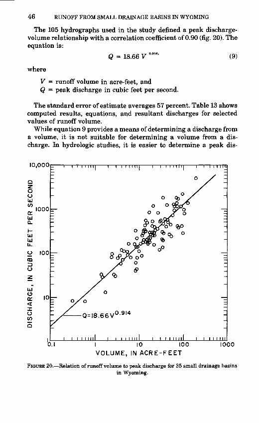
46 RUNOFF FROM SMALL DRAINAGE BASINS IN WYOMING
The 105 hydrographs used in the study defined a peak discharge- volume relationship with a correlation coefficient of 0.90 (fig. 20). The equation is:
Q = 18.66 V (9)
where
V = runoff volume in acre-feet, andQ = peak discharge in cubic feet per second.
The standard error of estimate averages 57 percent. Table 13 shows computed results, equations, and resultant discharges for selected values of runoff volume.
While equation 9 provides a means of determining a discharge from a volume, it is not suitable for determining a volume from a dis charge. In hydrologic studies, it is easier to determine a peak dis-
10,000
O oUJ
£1000UJ Q.
I- UJ UJu_o 100COID O
UJ
Xo
10
O.I
o/o
Q=I8.66V°- 914
I Mill
I 10 100 VOLUME, IN ACRE-FEET
1000
FIGURE 20. Relation of runoff volume to peak discharge for 35 small drainage basinsin Wyoming.
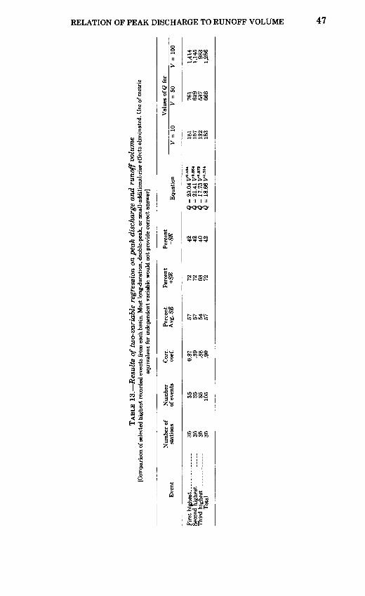
TABL
E 13.
Res
ults
of
two-
vari
able
reg
ress
ion
on p
eak
disc
harg
e a
nd
ru
no
ff v
olum
e[C
ompa
riso
n of
sele
cted
hig
hest
rec
orde
d ev
ents
fro
m e
ach
basi
n. M
ost l
ong-
dura
tion,
dou
ble-
peak
, or
smal
l-ad
ditio
nal-
rise
eff
ects
elim
inat
ed.
Use
of m
etri
ceq
uiva
lent
for
ind
epen
dent
var
iabl
e w
ould
not
pro
vide
cor
rect
ans
wer
]
Eve
nt
Tot
al ..- _.
Num
ber
ofst
atio
ns
35 35 35 35
Num
ber
Cor
r.of
eve
nts
coef
.
35
0.87
35
.89
35
.88
105
.90
Perc
ent
Avg
. SB
57 57 54 57
Perc
ent
+SE 72 72 68 72
Perc
ent
-SE
42 42 40 42
Equ
atio
n
O =
23.0
4 V
0-89
40
= 2
1.41
V0'
864
6 =
17
73 V
0-87
2Q
= 1
8.66
V0-
914
V =
10
181
157
132
153
Val
ues
of Q
foi
V =
50
761
629
537
666
V =
100
1,41
41,
145
983
1,25
6
i o o s as o
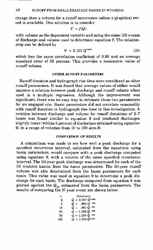
48 RUNOFF FROM SMALL DRAINAGE BASINS IN WYOMING
charge than a volume for a runoff occurrence unless a graphical rec ord is available. One solution is to consider
V = f(Q)
with volume as the dependent variable and using the same 105 events of discharge and volume used to determine equation 9. The relation ship can be defined by
V = 0.131 Q 0 -878 (10)
which has the same correlation coefficient of 0.90 and an average standard error of 55 percent. This provides a reasonable value of runoff volume.
OTHER RUNOFF PARAMETERS
Runoff duration and hydrograph rise time were considered as other runoff parameters. It was found that average values of either would improve a relation between peak discharge and runoff volume when used in a multiple regression. Although the improvement was significant, there was no easy way to estimate these two parameters for an ungaged site. Basin parameters did not correlate reasonably with runoff duration or hydrograph rise time in this investigation. A relation between discharge and volume for runoff durations of 2-7 hours was found similar to equation 9 and produced discharges slightly lower (within 5 percent of discharges obtained using equation 9) in a range of volumes from 10 to 100 acre-ft.
COMPARISON OF RESULTS
A comparison was made to see how well a peak discharge for a specified recurrence interval, estimated from the equations using basin parameters, would compare with a peak discharge computed using equation 9, with a volume of the same specified recurrence interval. The 50-year peak discharge was determined for each of the 22 modeled basins from the basin parameters. The 50-year runoff volume was also determined from the basin parameters for each basin. This value was used in equation 9 to determine a peak dis charge for each basin. The discharge computed from equation 9 was plotted against the Q50 estimated from the basin parameters. The results of comparing the N-year event are shown below:
N Relationship2 $ = 0.767 Q 0 -9635 0 = -905 Q 965
10 $ = -981 Q -97025 0 = 1-026 Q -98250 0 = 1-038 Q -"3
100 0 = 1-058 Q 1 -002
MEAN DIMENSIONLESS HYDROGRAPH 49
Statistically, for the 25-, 50, or 100-year event, there is no significant difference between the discharge estimated from basin parameters and the discharge computed from the equation relating to volume (equation 9). At the 5-percent level of significance, the slope of each relation is not significantly different from 1.00 and the intercept is not significantly different from zero. Relations for the 2-year, 5-year, and 10-year events are weaker, to the extent that equation 9 predicts higher discharges from the 2-year, 5-year, and 10-year runoff volumes. A weakness in the discharge-volume relation is that low- runoff occurrences reflect the variability of rainfall more than the high flows.
The relation between discharge and volume for the higher flows shows less scatter because these occurrences are more dependent on larger storms that cover the entire basin. Data from the larger storms were used in synthesizing the long-term runoff records used in the development of flow frequencies. The relations of flow frequencies to basin characteristics would therefore be more consistent in estimat ing specific frequencies of discharge or volume, especially the 2-year, 5-year, and 10-year events, from the basin characteristics.
This analysis indicates that for best results a design volume or discharge should be determined using basin characteristics in the appropriate mathematical model. If a hydrograph is needed for design purposes, the discharge and volume for the same design frequency should be used with the composite MDH method to develop the hy drograph, as described in subsequent sections.
MEAN DIMENSIONLESS HYDROGRAPH
Investigations of runoff resulting from rainfall on 28 small drain age basins in Wyoming indicate that a standard dimensionless hy drograph can be used to produce usable synthetic hydrographs of single-peak runoff occurrences. The 22 modeled basins and 6 other basins, all having a minimum of 7 usable hydrographs, were used to study hydrograph shape. As a result, mean dimensionless hydro- graphs were developed for individual drainage basins, following which a single composite mean dimensionless hydrograph was devel oped for the 28 drainage basins. The application of this hydrograph is similar to that of the Commons (1942) dimensionless hydrograph, which was based on floods in Texas and has been successfully com pared with observed hydrographs of floods in New York, Connecticut, Pennsylvania, and other areas. The Wyoming composite hydrograph (Craig, 1970) has produced synthetic hydrographs that compare well with observed runoff hydrographs from Wyoming, Arizona, and New Mexico. All streams used to develop and test the method are ephemeral.
50 RUNOFF FROM SMALL DRAINAGE BASINS IN WYOMING
COMPOSITE MEAN DIMENSIONLESS HYDROGRAPH
The peak discharge in cubic feet per second and the volume of runoff in acre-feet are needed to produce a synthetic hydrograph. Discharge and time-factor constants are determined from the peak discharge and volume of recorded hydrographs. The constants then are multiplied by increments of discharge and time from the dimen- sionless hydrograph to obtain the plotting points of the synthetic hydrograph. The synthetic peak discharge always has the same value as the actual peak; therefore, the peak must be known.
Commons' dimensionless hydrograph, developed empirically, used a horizontal (time) scale of 100 units and a vertical (rate-of-flow) scale of 60 units. The area under the curve was 1,196.5 "square units" (time units multiplied by rate-of-flow units). The value of one "square unit" in acre-feet was obtained by dividing the total floodflow (volume) in acre-feet by 1,196.5. The value of one unit of flow in cubic feet per second was obtained by dividing the peak flow in cubic feet per second by 60. The rising limb and recession limb of the Commons hydro- graph appear characteristic of most streams, large or small, but the long recession is more indicative of large streams that are sustained by flow returning from overflow or storage on flood plains or from ground water in the stream banks.
The ephemeral streams investigated in this Wyoming study do not reflect this large storage effect; consequently, a few changes were made in developing a mean dimensionless hydrograph for each stream. In order to produce a characteristic hydrograph shape of small ephemeral streams in semiarid areas, an arbitrary value of 1,000 square units was used for the volume, and Commons' value for the peak was retained as 60 flow units. However, unlike the Com mons method, in which the time scale was fixed, time was allowed to vary with the magnitude of the runoff occurrence. An average time value was determined for each dimensionless hydrograph. The values for volume, peak discharge, and time were used to convert individual observed runoff hydrographs to dimensionless form.
A dimensionless hydrograph was developed for each site by averag ing points on the abscissa (time scale) at selected ordinate (discharge scale) points. These 28 dimensionless hydrographs were combined by averaging abscissa points for selected ordinate points, making a smooth final composite hydrograph. Finally, ordinate points were de termined for selected abscissa points to best describe the composite mean dimensionless hydrograph. A total of 298 hydrographs from the 28 drainage basins were used to develop the final composite hydro- graph. The planimetered volume was 970 square units with a rise time of 12 time units. The average time of the base was 70 time units.
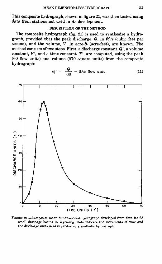
MEAN DIMENSIONLESS HYDROGRAPH 51
This composite hydrograph, shown in figure 21, was then tested using data from stations not used in its development.
DESCRIPTION OF THE METHOD
The composite hydrograph (fig. 21) is used to synthesize a hydro- graph, provided that the peak discharge, Q, in ft3/s (cubic feet per second), and the volume, V, in acre-ft (acre-feet), are known. The method consists of two steps. First, a discharge constant, Q', a volume constant, V, and a time constant, T' , are computed, using the peak (60 flow units) and volume (970 square units) from the composite hydrograph:
Q' = = ft3/s flow unit (11)
10 20 30 40
TIME UNITS (t')50 60 70
FIGURE 21. Composite mean dimensionless hydrograph developed from data for 28 small drainage basins in Wyoming. Dots indicate the increments of time and the discharge units used in producing a synthetic hydrograph.
52 RUNOFF FROM SMALL DRAINAGE BASINS IN WYOMING
V = - = acre-ft per square unit, and (12)*J i \)
T' = 726 -¥ = min per time unit, (13) Q
where square units = flow units x time units, and 726 is a constant for converting acre-feet to cubic feet and seconds to minutes.
The second step is to compute the actual plotting points, t and q, for the synthetic hydrograph. Sixteen plotting points were selected to define the entire hydrograph, as shown in figure 21. The coordinates of these points on the composite hydrograph in figure 21 are desig nated ait' andq'. Once a set of values of t' andq' has been selected, it is used in synthesizing every new hydrograph. For each of the 16 points
t = t'T', and (14) q = q'Q', (15)
wheret is time in minutes,t' is time in units,q is discharge in cfs,q' is flow units, andT' and Q' are as previously defined.
The values of t' andq' are strictly empirical and define the composite hydrograph.
The method can best be shown by developing a synthetic hydro- graph for an actual runoff occurrence. On June 10, 1965, a peak flow was recorded on Pritchard Draw near Lance Creek, in eastern Wyom ing. The peak discharge was 1,280 ft3/s and the volume was computed as 67.17 acre-feet. From equations 11, 12, and 13, Q', V, and T' were determined as follows:
Q' = = 21.33 ft3/s per flow unit,
V = 6J7 Q7 = 0.069 acre-ft per sq unit, and
T' = 726 - = 726 x -r = 2.35 min per time unit.(cf &1.OO
Selected increments of time units, t' (table 14), and corresponding discharge units, q', the 16 points shown in figure 21, are multiplied by constants T' and Q', respectively, to determine the time, t, and cor responding discharge, q, for points on the synthetic hydrograph. The listed values of t' and q' were used in synthesizing all hydrographs shown in this report.
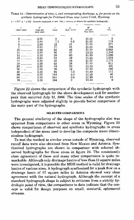
MEAN DIMENSIONLESS HYDROGRAPH 53
TABLE 14. Determination of time, t, and corresponding discharge, q, for points on the synthetic hydrograph for Pritchard Draw near Lance Creek, Wyoming
[t = t'XT'; q = q'XQ'. Symbols explained in text. Plot t versus q to obtain the synthetic hydrograph]
t' (time units)
0 _ _357 _ ___.
10 ______ .11 _______1213 _______14 ________18 __ ___ .23 _______30 _______40 ________50 _______60 _______70 _______
T' (min per
time unit)
2.352.352.352.352.352.352.352.352.352.352.352.352.352.352.352.35
t(min)
07.1
1217242628313342547094
118141164
?'(flow units)
05.6
132549576059553823125.22.00.50
Q'(cfs per
flow unit)
21.3321.3321.3321.3321.3321.3321.3321.3321.3321.3321.3321.3321.3321.3321.3321.33
(cfs)
0119211533
1,0451,2161,2801,2581,173
8114912561114311
0
Figure 22 shows the comparison of the synthetic hydrograph with the observed hydrograph for the above development and for another peak that occurred July 13, 1966. The time scales of the synthetic hydrographs were adjusted slightly to provide better comparison of the main part of the hydrographs.
SELECTED COMPARISONS
The general similarity of the shape of the hydrographs also was apparent from comparisons in other areas in Wyoming. Figure 23 shows comparisons of observed and synthetic hydrographs in areas independent of the areas used to develop the composite mean dimen- sionless hydrograph.
To test the method in similar areas outside of Wyoming, observed runoff data were also obtained from New Mexico and Arizona. Syn thesized hydrographs are shown in comparison with selected ob served hydrographs for these areas in figure 24. The consistently close agreement of these and many other comparisons is quite re markable. Although only drainage basins of less than 11 square miles were investigated, it is possible the MDH method is valid for drainage basins of various sizes. A hydrograph synthesized for a peak flow on a drainage basin of 57 square miles in Arizona showed very close agreement with the natural hydrograph. Although the concept of a standard hydrograph shape is subject to criticism from a strictly hy- drologic point of view, the comparisons to date indicate that the con cept is valid for design purposes on small, semiarid, ephemeral streams.
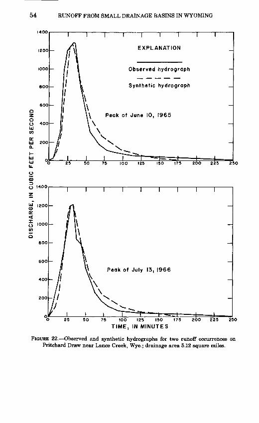
54 RUNOFF FROM SMALL DRAINAGE BASINS IN WYOMING
1400
1200
I I I I
EXPLANATION
Observed hydrograph
Synthetic hydrograph
Peak of June 10, 1965
50 75 100 125 150 175 200 225 250
Peak of July 13, 1966
25 50 75 100 125 150 175 200 225 250
TIME, IN MINUTES
FIGURE 22. Observed and synthetic hydrographs for two runoff occurrences on Pritchard Draw near Lance Creek, Wyo.; drainage area 5.12 square miles.
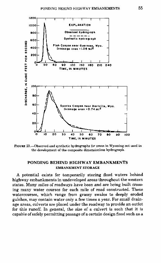
PONDING BEHIND HIGHWAY EMBANKMENTS 55
1200
1000
800
600
400
200
i i I rEXPLANATION
Observed hydrograph
Synthetic hydrogroph
Fish Canyon near Guernsey, Wyo. Drainage area = 1.06 ml 2
30 60 90 120 ISO ISO 210 240 TIME, IN MINUTES
Sparks Canyon near Hartville, Wyo. Drainage area =0.74 mi 2
10 20 30 40 50 60 70 SO 90 100 TIME, IN MINUTES
FIGURE 23. Observed and synthetic hydrographs for areas in Wyoming not used in the development of the composite dimensionless hydrograph.
PONDING BEHIND HIGHWAY EMBANKMENTS EMBANKMENT STORAGE
A potential exists for temporarily storing flood waters behind highway embankments in undeveloped areas throughout the western states. Many miles of roadways have been and are being built cross ing many water courses for each mile of road constructed. These watercourses, which range from grassy swales to deeply eroded gulches, may contain water only a few times a year. For small drain age areas, culverts are placed under the roadway to provide an outlet for this runoff. In general, the size of a culvert is such that it is capable of safely permitting passage of a certain design flood such as a
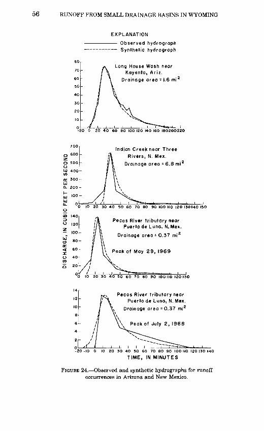
56 RUNOFF FROM SMALL DRAINAGE BASINS IN WYOMING
EXPLANATION
Observed hydrograph Synthetic hydrograph
Long House Wash nearKayenta, Ariz.
Drainage area - 1.6 mi'
0 20 40 60 60 100 120 140 160 180200220
Indian Creek near ThreeRivers, N. Mex.
Drainage area = 6.8 mi'
20 30 40 50 60 70 80 90 100 110 120 I3OI40 150
Pecos River tributary near Puerto de Luna, N. Mex.
Drainage areo = 0.37 mi 2
v Peak of May 29, 1969
20 30 40 50 60 70 80 90 100 110 120130
Pecos River tributary nearPuerto de Luna, N. Mex.
Drainage area = 0.37 mi 2
Peak of July 2, 1968
-20-10 0 IO 20 30 40 50 60 70 80 90 100 110 120 130 140
TIME, IN MINUTES
FIGURE 24. Observed and synthetic hydrographs for runoff occurrences in Arizona and New Mexico.
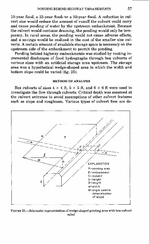
PONDING BEHIND HIGHWAY EMBANKMENTS 57
10-year flood, a 25-year flood- "or a 50-year flood. A reduction in cul vert size would reduce the amount of runoff the culvert could carry and cause ponding of water by the upstream embankment. Because the culvert would continue draining, the ponding would only be tem porary. In rural areas, the ponding would not cause adverse effects, and a savings would be realized in the cost of the smaller size cul verts. A certain amount of available storage space is necessary on the upstream side of the embankment to permit the ponding.
Ponding behind highway embankments was studied by routing in cremental discharges of flood hydrographs through box culverts of various sizes with an artificial storage area upstream. The storage area was a hypothetical wedge-shaped area in which the width and bottom slope could be varied (fig. 25).
METHOD OF ANALYSIS
Box culverts of sizes 4 x 4 ft, 5 x 5 ft, and 6 x 6 ft were used to investigate the flow through culverts. Critical depth was assumed at the culvert entrance to avoid assumptions of other culvert features such as slope and roughness. Various types of culvert flow are de-
= ponding oreo
E= embonkment C= culvert h = height jMength w=width -6-=ongle used in
determinationof slope
FIGURE 25. Schematic representation of wedge-shaped ponding area with box-culvertrelief.
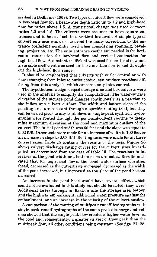
58 RUNOFF FROM SMALL DRAINAGE BASINS IN WYOMING
scribed in Bodhaine (1968). Two types of culvert flow were considered. A low-head flow for a headwater depth ratio up to 1.2 and high-head flow for ratios above 1.5. A transitional change was used between ratios 1.2 and 1.5. The culverts were assumed to have square en trances and to be set flush in a vertical headwall. A simple type of culvert entrance was used to avoid the many corrections to the en trance coefficient normally used when considering rounding, bevel ing, projection, etc. The only entrance coefficient needed is for hori zontal contraction for low-head flow and vertical contraction for high-head flow. A constant coefficient was used for low-head flow and a variable coefficient was used for the transition flow to and through out the high-head flow range.
It should be emphasized that culverts with outlet control or with flows changing from inlet to outlet control can produce reactions dif fering from this analysis, which concerns only inlet control.
The hypothetical wedge-shaped storage area and box culverts were used in the analysis to simplify the computations. The water-surface elevation of the storage pond changes continuously as a reaction to the inflow and culvert outflow. The width and bottom slope of the ponding area are constant through a specific routing trial, but they can be varied prior to any trial. Several single-peak synthetic hydro- graphs were routed through the pond-and-culvert routine to deter mine maximum elevation of the pond and maximum outflow of the culvert. The initial pond width was 60 feet and the slope was equal to 0.02 ft/ft. Other tests were made for an increase of width to 100 feet or an increase in slope to 0.03 ft/ft. Routing tests were made for all three culvert sizes. Table 15 contains the results of the tests. Figure 26 shows culvert discharge rating curves for the culvert sizes investi gated, as determined from the data of table 15. The reactions to in creases in the pond width and bottom slope are noted. Results indi cated that for high-head flows, the pond water-surface elevation (head) decreased as the culvert size increased, decreased as the width of the pond increased, but increased as the slope of the pond bottom increased.
An increase in the pond head would have several effects which could not be evaluated in this study but should be noted; they were: Additional losses through infiltration into the storage area bottom and the highway embankment, additional water pressure against the embankment, and an increase in the velocity of the culvert outflow.
A comparison of the routing of multipeak runoff hydrographs with single-peak runoff hydrographs of the same peak discharge and vol ume showed that the single-peak flow creates a higher water level in the pond and, consequently, a greater culvert outflow peak than the multipeak flow, all other conditions being constant. (See figs. 27, 28,
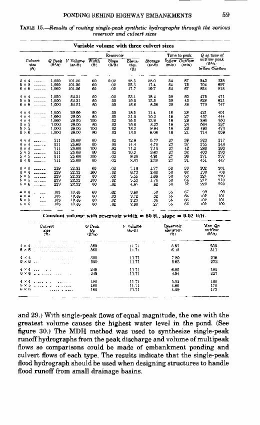
PONDING BEHIND HIGHWAY EMBANKMENTS 59
TABLE 15. Results of routing single-peak synthetic hydrographs through the variousreservoir and culvert sizes
Variable volume with three culvert sizes
ReservoirCulvert
size(ft)
4x4 _5x5 _____6x6
4x4 __ _5x5 ____6x6 _ __
4X4 _____4X4 _____4x4 _____5x55x5 ____6x6 _____
4x4 --.__4x4 __ _.4x4 __5x5 _____5x5 _____6x6 _____
4X4 _ _4X4 ___5x55x56x6 __ _
4X4 _____4x4 ._ _5x56x6 ___.
QPeak(ft3/s)
_ 1,0001,000
_ 1,000
_ 1,000_ 1,000_ 1,000
_ 1,000_ 1,000_ 1,000_ 1.000_ 1,000_ 1,000
511511511511511511
229229229229229
103103103103
V Volume(ac-ft)
101.26 101.26 101.26
54.21 54.21 54.21
29.00 29.00 29.00 29.00 29.00 29.00
25.66 25.66 25.66 25.66 25.66 25.66
22.32 22.32 22.32 22.32 22.32
10.48 10.48 10.48 10.48
Width (ft)
60 60 60
60 60 60
60 60
100 60
100 60
60 60
100 60
100 60
60 100 60
100 60
60 60 60 60
Slope (ft/ft)
0.02 .02 .02
.02
.02
.02
.02
.03
.02
.02
.02
.02
.02
.03
.02
.02
.02
.02
.02
.02
.02
.02
.02
.02
.03
.02
.02
Eleva tion (ft)
28.5 22.5 17.7
23.1 19.0 15.6
18.2 21.0 15.0 15.5 13.2 13.3
12.9 14.4 11.2 10.2 9.25 8.31
7.16 6.73 5.55 5.53 4.87
3.80 3.72 3.23 2.80
Storage (ac-ft)
28.0 17.4 10.7
18.4 12.5 8.38
11.4 10.2 12.9
8.27 9.94 6.06
5.77 4.78 7.15 3.61 4.91 2.38
1.77 2.60 1.06 1.76
.82
.50
.32
.36
.27
Time to peakInflow (min)
54 54 54
29 29 29
16 16 16 16 16 16
27 27 27 27 27 27
50 50 50 50 50
55 55 55 55
Outflow (min)
87 75 67
50 43 38
28 27 29 24 26 21
39 37 42 34 36 31
59 62 53 56 52
57 56 56 56
Q at time of outflow peak
(ft3/S,
Inflow Outflow
543 704 824
475 628 770
421 457 386 564 493 714
323 355 286 403 371 451
202 190 221 212 223
99 102 102 102
538 697 818
471 621747
401 444 350 537 473 659
317 344 283 393 357 447
201 188 220 210 223
99 101 101 102
Constant volume with reservoir width = 60 ft., slope = 0.02 ft/ft.
Culvert size (ft)
4x4 _________ _ ___6x6 _ _ ___ _______ ____
4x4 ______6x6 .__ _ _______ _ _ __
4x4 ___ _____ ___ _ _ _.6 x 6 _ _ _ _
4x4 _____ _ _ _____ _5 x 5 ______ _ 6x6 _____
QPeak Qp
(ft3/s)
360360
300300
249249
180180 180
V Volume (ac-ft)
11.71
11.71
11.71 11.71
Reservoir elevation
(ft)
6.15
7 805.62
5.524.66 4.09
Max. Qp outflow(ft3/s)
233311
272
195227
160170 173
and 29.) With single-peak flows of equal magnitude, the one with the greatest volume causes the highest water level in the pond. (See figure 30.) The MDH method was used to synthesize single-peak runoff hydrographs from the peak discharge and volume of multipeak flows so comparisons could be made of embankment ponding and culvert flows of each type. The results indicate that the single-peak flood hydrograph should be used when designing structures to handle flood runoff from small drainage basins.
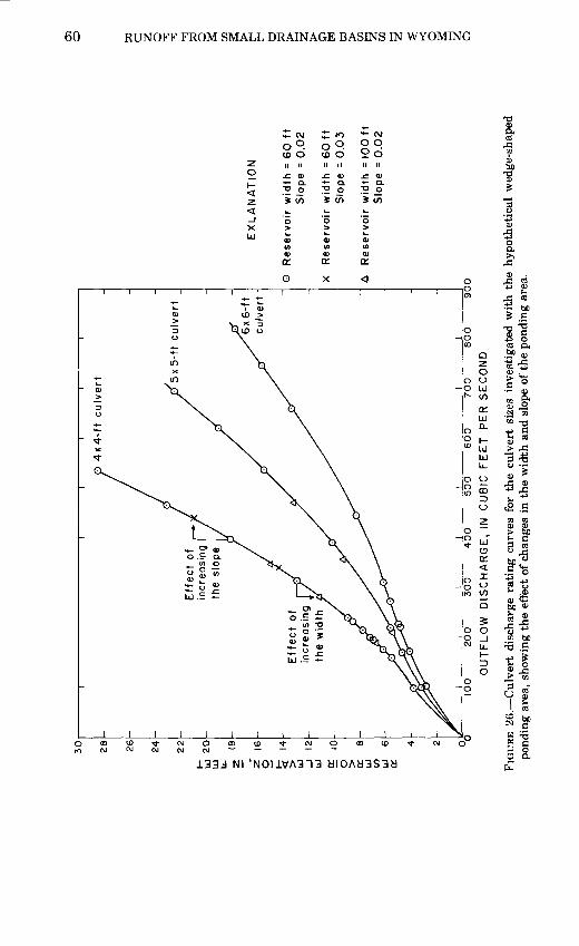
Eff
ect
of
incr
ea
sin
g
the
slo
pe
Effect
of
incr
ea
sin
g
the w
idth
EX
LA
NA
TIO
N
O
Rese
rvoir w
idth
= 6
0 f
t S
lope =
0.0
2
x
Re
serv
oir
wid
th
= 6
0 f
t S
lop
e =
0.0
3
A
Rese
rvoir
wid
th
= 10
0 ft
Slo
pe
=
0.0
2
100
20
0
30
0
400
50
0
600
70
0
800
OU
TF
LO
W
DIS
CH
AR
GE
, IN
C
UB
IC
FE
ET
P
ER
S
EC
ON
D
900
O5 O el
2
O *J *J *J
»
O s CO 25
>
O
H tti
>
CO 5 CO § 3 H< O
S §
O
FIG
URE
26. C
ulv
ert
disc
harg
e ra
ting
cur
ves
for
the
culv
ert
size
s in
vest
igat
ed w
ith
the
hypo
thet
ical
wed
ge-s
hape
d po
ndin
g ar
ea,
show
ing
the
effe
ct o
f ch
ange
s in
the
wid
th a
nd s
lope
of
the
pond
ing
area
.
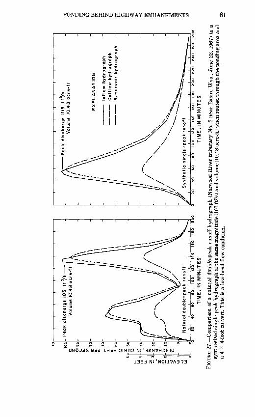
±
3H
"
O
UJ
I-J UJ
O 9
0c U
J U
. 6
0
UJ CD cn s
o
Pea
k dis
charg
e
103
ft /s
Volu
me 1
0.48
acre
-ft
Na
turo
l d
ou
ble
-pe
ok
run
off
60
eO
100
120
140
TIM
E,
IN M
INU
TE
S16
0 16
0 2
00
Pe
ak
dis
ch
arg
e
103
ft*/
sV
olu
me
10.4
8 a
cre
-ft
EX
PL
AN
AT
ION
Inflo
w h
yd
rog
rap
h
Outflo
w h
yd
rog
rap
h
Re
se
rvo
ir hydro
gra
ph
Syn
the
tic s
ingle
100
120
140
160
ICO
TIM
E,
IN M
INU
TE
S200
220
24
0
26
0
26
0
FIG
URE
27.
Com
pari
son
of a
nat
ural
dou
ble-
peak
run
off
hydr
ogra
ph (
Nor
woo
d R
iver
tri
buta
ry N
o. 2
nea
r B
asin
, W
yo.,
June
22,
196
7) t
o a
synt
hesi
zed
sing
le-p
eak
hydr
ogra
ph o
f the
sam
e m
agni
tude
(10
3 ft
3/s)
and
vol
ume
(10.
48 a
cre-
ft)
whe
n ro
uted
thro
ugh
the
pond
ing
area
and
a
4 x
4-fo
ot c
ulve
rt.
Thi
s is
a l
ow-h
ead
flow
con
ditio
n.
s § I-H
2 O
td
M
ffi
§ a ffi o ffi Cd CO
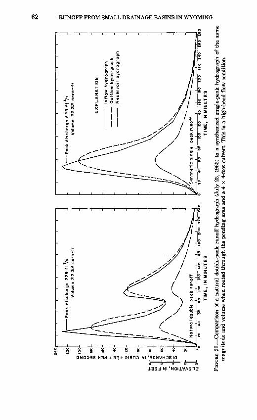
O5 to
UJ
UJ *1 1- <
2
UJ
UJ
0
§2
00
o
o 111
ISO
CO a: 11
1 16
0
UJ
140
UJ U.
O
100
z o
cc -<
60
O
CO --
40
Pe
ak
dis
charg
e 229 f
t 3/s
Vol
ume
22
.32
acre
-ft
80
10
0 12
0 1
40
160
ISO
2
00
220
240
TIM
E,
IN M
INU
TE
S
-Pea
k dis
charg
e 2
29 f
t /s
Vol
ume
22.3
2 acre
-ft
EX
PL
AN
AT
ION
Inflo
w h
ydro
gra
ph
Ou
tflo
w h
ydro
gra
ph
Rese
rvoir h
ydro
gra
ph
40
60
80
100
120
140
160
ISO
2
00
220
240
26
0
280
TIM
E,
IN M
INU
TE
S
FIG
URE
28.
Com
pari
son
of a
nat
ural
dou
ble-
peak
run
off
hydr
ogra
ph (
July
25,
196
5) t
o a
synt
hesi
zed
sing
le-p
eak
hydr
ogra
ph o
f th
e sa
me
mag
nitu
de a
nd v
olum
e w
hen
rout
ed t
hrou
gh t
he p
ondi
ng a
rea
and
a 4
x 4-
foot
cul
vert
. T
his
is a
hig
h-he
ad f
low
con
ditio
n.
i CO I £2 CO 5 i I I 2 Q
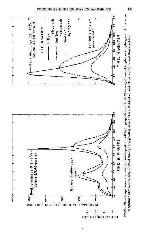
LJ
LJ
15
Z
10
60
0
§
500
O o U
J (O <r U
J 4
00
a. UJ
LJ
U.
O
30
0
CD 13
O UJ
ZO
Oe> (T o (O -
10
0
Pea
k dis
charg
e
511
ft 3/s
V
olum
e 25,6
6 a
cre
-ft
Na
tura
l double
-peak
runoff
20
40
60
80
10
0
120
140
160
180
20O
TIM
E,
IN
MIN
UT
ES
\ P
eak d
isch
arg
e
511
ft3/s
Vol
ume
25.6
6 a
cre
-ft
EX
PL
AN
AT
ION
Inflo
w hydr
ogra
ph
Outflo
why
drog
raph
.
Re
serv
oir
hydr
ogra
ph
Synth
etic s
lngle
- \
peak
ru
no
ff
\ \
40
60
60
10
0
120
TIM
E,
IN
MIN
UT
ES
140
160
FIG
URE
29.
Com
pari
son
of a
nat
ural
dou
ble-
peak
run
off
hydr
ogra
ph (
June
14,
196
7) t
o a
synt
hesi
zed
sing
le-p
eak
hydr
ogra
ph o
f th
e sa
me
mag
nitu
de a
nd v
olum
e w
hen
rout
ed t
hrou
gh t
he p
ondi
ng a
rea
and
a 4
x 4-
foot
cul
vert
. T
his
is a
hig
h-he
ad f
low
con
ditio
n.C
O
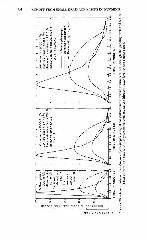
ELEVATION, IN FEET
DISCHARGE, IN CUBIC FEET PER SECOND
mCO CD
5 5 H om co -
ONIWOAM NI SNISV9 3DVNIVHQ 11VWS
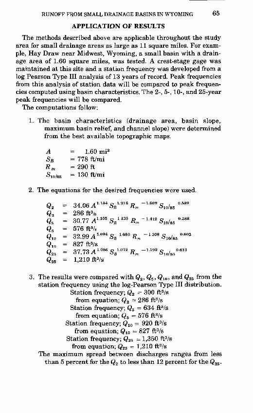
RUNOFF FROM SMALL DRAINAGE BASINS IN WYOMING 65
APPLICATION OF RESULTS
The methods described above are applicable throughout the study area for small drainage areas as large as 11 square miles. For exam ple, Hay Draw near Midwest, Wyoming, a small basin with a drain age area of 1.60 square miles, was tested. A crest-stage gage was maintained at this site and a station frequency was developed from a log Pearson Type III analysis of 13 years of record. Peak frequencies from this analysis of station data will be compared to peak frequen cies computed using basin characteristics. The 2-, 5-, 10-, and 25-year peak frequencies will be compared.
The computations follow:
1. The basin characteristics (drainage area, basin slope, maximum basin relief, and channel slope) were determined from the best available topographic maps.
A = 1.60 mi2Sg = 778 ft/miR m =290 ftS10/85 = 130 ft/mi
2. The equations for the desired frequencies were used.
Q2 = 3Q2 = 286ft3/sQ QA 77 ,41.105 c 1.135 p 1.412 c / 0.588
5 OU. / / A SB ttm £>io/85
Q5 = 576ft3/S
Q QO QQ A I- 094 C I 080 I? 1308 Q . 0.603 10 ~ O^.yy A OB fi m ^10/85
Q 10 = 827 ft3/sQ OT 70 yl 1-086 c 1012 T-> 1.192 o . 0.613
25 6 I. 16 A 5S Xt m 010/85
Qas = 1,210 ft3/s
The results were compared with Q2 , Q5 , Qio > and Q25 from the station frequency using the log-Pearson Type III distribution.
Station frequency; Q2 = 300 ft3/sfrom equation; Q2 =286 ft3/s
Station frequency; Q5 = 634 ft3/sfrom equation; Q5 = 576 ft3/s
Station frequency; Q 10 = 920 ft3/s from equation; Q 10 = 827 ft3/s
Station frequency; Q25 = 1,350 ft3/sfrom equation; Q25 = 1,210 ft3/s
The maximum spread between discharges ranges from less than 5 percent for the Q2 to less than 12 percent for the Q25 .
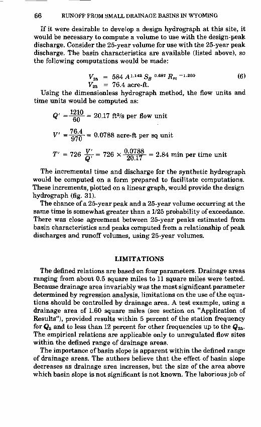
66 RUNOFF FROM SMALL DRAINAGE BASINS IN WYOMING
If it were desirable to develop a design hydrograph at this site, it would be necessary to compute a volume to use with the design-peak discharge. Consider the 25-year volume for use with the 25-year peak discharge. The basin characteristics are available (listed above), so the following computations would be made:
V25 = 584 A 1 - 142 SB °-687 Rm ~ 1 - 260 (6) V2S = 76.4 acre-ft.
Using the dimensionless hydrograph method, the flow units and time units would be computed as:
Q' =±^~= 20.17 ft3/s per flow unit
V = ®'Q = 0.0788 acre-ft per sq unit
T = 726 ^- = 726 x ^Qll = 2 '84 min per time unit
The incremental time and discharge for the synthetic hydrograph would be computed on a form prepared to facilitate computations. These increments, plotted on a linear graph, would provide the design hydrograph (fig. 31).
The chance of a 25-year peak and a 25-year volume occurring at the same time is somewhat greater than a 1/25 probability of exceedance. There was close agreement between 25-year peaks estimated from basin characteristics and peaks computed from a relationship of peak discharges and runoff volumes, using 25-year volumes.
LIMITATIONS
The defined relations are based on four parameters. Drainage areas ranging from about 0.5 square miles to 11 square miles were tested. Because drainage area invariably was the most significant parameter determined by regression analysis, limitations on the use of the equa tions should be controlled by drainage area. A test example, using a drainage area of 1.60 square miles (see section on "Application of Results"), provided results within 5 percent of the station frequency for Q2 and to less than 12 percent for other frequencies up to the QK . The empirical relations are applicable only to unregulated flow sites within the defined range of drainage areas.
The importance of basin slope is apparent within the defined range of drainage areas. The authors believe that the effect of basin slope decreases as drainage area increases, but the size of the area above which basin slope is not significant is not known. The laborious job of
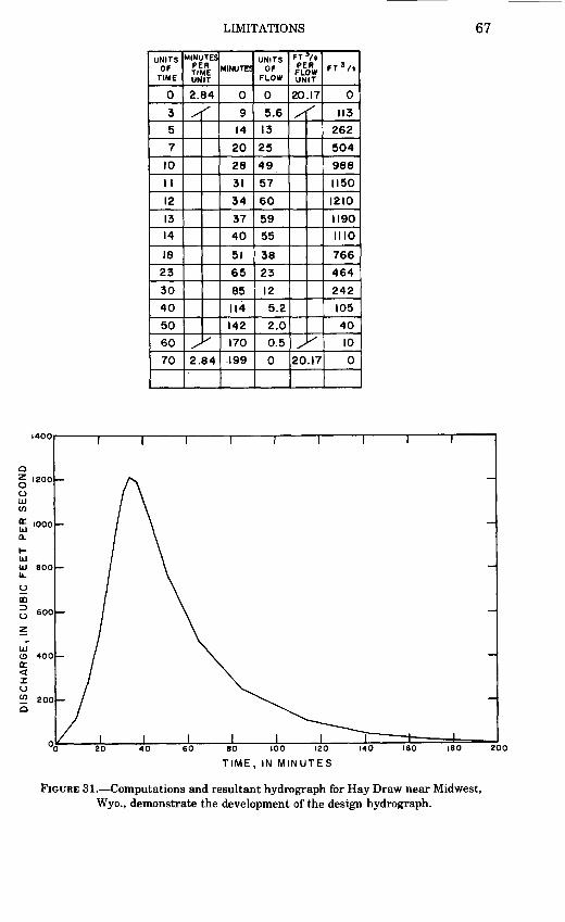
LIMITATIONS 67
UNITS OF
TIME
0
3
5
7
10
II
12
13
14
18
23
30
40
50
60
70
MINUTES PER TIME UtilT
2.84
x
/
^
X
2.84
MINUTES
0
9
14
20
28
31
34
37
40
51
65
85
114
142
170
J99
UNITS OF
FLOW
0
5.6
13
25
49
57
60
59
55
38
23
12
5.2
2.0
0.5
0
FT 3/* PER
FLOW UNIT
20.17
xl
/
s
/
20.17
FT 3 /s
0
113
262
504
988
1150
1210
1190
1110
766
464
242
105
40
10
0
1400
1200
UJUJ 800U.
UJO 400(E<Io<f> 200 O
TIME, IN MINUTES
FIGURE 31. Computations and resultant hydrograph for Hay Draw near Midwest, Wyo., demonstrate the development of the design hydrograph.
68 RUNOFF FROM SMALL DRAINAGE BASINS IN WYOMING
determining basin slope for larger basins would be a deterrent to proving this hypothesis. Maximum basin relief, having only a small effect on small drainage areas, might be ineffective on larger ones. Main-channel slope appears to have a minor effect on small drainage basins but apparently becomes more effective on larger basins; the size of area beyond which main-channel slope begins to be effective is not known. Benson (1962) found main-channel slope to be significant and generally second to drainage area in its effect on peak discharge for all sizes of drainage areas in New England.
The use of the mean dimensionless hydrograph would be limited only to the extent of obtaining a runoff volume for a peak flow. In this study the defined relations for estimating volume are limited to 11 square miles or smaller. The mean dimensionless hydrograph method was developed from hydrographs of runoff events on small drainage basins. The method is similar to Commons' (1942) dimensionless hy drograph which was developed from hydrographs for large drainage basins. The main differences in the two methods is that the recession is reduced for the small basins and, consequently, the area under the hydrograph is smaller for the small basins.
SUMMARY AND CONCLUSIONS
This study has shown that long-term runoff records can be synthe sized from long-term rainfall records; that the dimensionless hydro- graph method can provide a standardize hydrograph shape for use in designing culverts and bridges; and that the potential for temporarily storing flood waters behind highway embankments in undeveloped areas can be economically beneficial.
Methods and techniques were applied or developed as follows to accomplish the objectives of this research project.
1. A rainfall-runoff model and a long-term rainfall record (73 years at Cheyenne, Wyo.) were used to synthesize long-term runoff records of annual peak discharges and volumes for 22 small drainage basins in Wyoming. The process involved calibrating a model to each basin from rainfall and runoff observations on each basin. Daily rainfall data from nearby stations of the National Weather Service were used to determine antecedent conditions. Model parameters were developed that best relate the rainfall and runoff. The long- term rainfall record was then used with the model parame ters to generate a long-term runoff record on each basin. Variations between Cheyenne and the study basin due to orographic effects were considered and adjustments were applied to the long-term rainfall for transfer to each basin.
SELECTED REFERENCES 69
2. Volume and peak frequencies were defined at each of the 22 sites through log-Pearson Type III analysis of each synthe sized 73-year record.
3. Runoff frequencies of 2, 5, 10, 25, 50, and 100 years were re lated to basin characteristics, using regression techniques. The basin characteristics most significant in relating vol ume frequencies were drainage area, maximum basin relief, and basin slope. Those most significant in relating peak frequencies were drainage area, basin slope, maximum basin relief, and channel slope.
4. A relationship between peak discharge and runoff volume was developed for determining a discharge from any volume. The relationship (Q = 18.66 Vn°<914) was defined from 105 runoff occurrences on 35 gaged sites (three hydrographs per site). A correlation coefficient of 0.90 was determined and an average standard error of estimate of 57 percent. The relationship was tested by substituting the volume frequen cies (2- to 100-year recurrence intervals) determined from the relationships using basin characteristics. The computed discharges were compared with the peak frequencies de termined from relationships using basin characteristics. The equation Q = 18.66 Vn° -914 predicts higher peaks from the 2-, 5-, and 10-year volumes than are estimated from basin characteristics. Peaks predicted from the 25-, 50-, and 100-year volumes are very close to those estimated from basin characteristics.
5. A dimensionless hydrograph was developed to define the characteristic shape of flood hydrographs. A peak discharge and a runoff volume are necessary to produce a synthetic hydrograph that is always a single-peak hydrograph.
6. Analyses of embankment storage indicate that the fast-rising single-peak runoff occurrence is most important in culvert design. Synthetic single-peak hydrographs developed from peaks and volumes of multipeak runoffs and routed through a culvert in an embankment caused higher water-surface elevations behind the embankment than did the natural multipeak flows.
SELECTED REFERENCES
Benson, M. A., 1962, Factors influencing the occurrence of floods in a humid region of diverse terrain: U.S. Geol. Survey Water-Supply Paper 1580-B, 64 p.
Bodhaine, G. L., 1968, Measurements of peak discharge at culverts by indirect methods: U.S. Geol. Survey Techniques of Water-Resources Inv., book 3, chap. A3, 60 p.
70 RUNOFF FROM SMALL DRAINAGE BASINS IN WYOMING
Butler, E., Reid, J. K., and Berwick, V. K., 1966, Magnitude and frequency of floods inthe United States, Part 10, the Great Basin: U.S. Geol. Survey Water-SupplyPaper 1684, 256 p.
Carter, J. R., and Green, A. R., 1963, Floods in Wyoming, magnitude and frequency:U.S. Geol. Survey Circ. 478, 27 p.
Chow, V. T., 1964, Handbook of applied hydrology: New York: McGraw-Hill Book Co.,section 4, part II, p. 39-76.
Commons, G. G., 1942, Flood hydrographs: Civil Eng., v. 12, no. 10, p. 571-572. Craig, G. S., Jr., 1970, Synthesizing hydrographs for small semiarid drainage basins, in
U.S. Geological Survey Research, 1970: U.S. Geol. Survey Prof. Paper 700-D, p.D238-D243.
Crawford, N. H., and Linsley, R. K., 1966, Digital similation in hydrology: Stanford,Calif., Stanford Watershed Model IV, Tech. Rept. 39, Civil Eng. Dept., StanfordUniv., 210 p.
Crow, E. L., Davis, F. A., and Maxfield, M. W., 1960, Statistics manual: New York,Dover Publications, 288 p.
Dalrymple, Tate, and Benson, M. A., 1967, Measurement of peak discharge by theslope-area method: U.S. Geol. Survey Techniques of Water-Resources Inv., book 3,chap. A2, 12 p.
Dawdy, D. R., Lichty, R. W., and Bergmann, J. M., 1972, A rainfall-runoff simulationmodel for estimation of flood peaks for small drainage areas: U.S. Geol. SurveyProf. Paper 506-B, 28 p.
Ezekiel, Mordecai, and Fox, K. A., 1959, Methods of correlation and regressionanalysis: New York, John Wiley and Sons, 548 p.
Linsley, R. K.,Kohler, M. A., and Paulhus, J. L., 1958, Hydrology for engineers: NewYork, McGraw-Hill Book Co. 340 p.
Lowham, H. W., 1976, Techniques for estimating flow characteristics of Wyomingstreams: U.S. Geol. Survey Water Resources Inv. 76-112, 83 p.
Matalas, N. C., and Benson, M. H., 1961, Effect of interstation correlation on regressionanalysis: Jour. Geophys. Research, v. 66, no. 10, p. 3285-3293.
Matthai, H. F., 1968, Magnitude and frequency of floods in the United States, Part 6-B,Missouri River basin below Sioux City, Iowa: U.S. Geol. Survey Water-SupplyPaper 1680, 491 p.
National Oceanic and Atmospheric Administration, 1974, Precipitation frequencyatlas of western United States: Atlas 2, v. II, 43 p.
Patterson, J. L., 1966, Magnitude and frequency of floods in the United States, Part6-A, Missouri River basin above Sioux City, Iowa: U.S. Geol. Survey Water- Supply Paper 1679, 471 p.
Patterson, J. L., and Somers, W. P., 1966, Magnitude and frequency of floods in theUnited States, Part 9, Colorado River basin: U.S. Geol. Survey Water-SupplyPaper 1683, 475 p.
Riggs, H. C., 1968, Some statistical tools in hydrology: U.S. Geol. Survey Techniques ofWater-Resources Inv., book 4, chap. Al, 39 p.
1973, Regional analyses of streamflow characteristics: U.S. Geol. Survey Tech niques of Water-Resources Inv., book 4, chap. B3, 15 p.
Thomas, C. A., Broom, H. C., and Cummans, J. E., 1963, Magnitude and frequency offloods in the United States, Part 13, Snake River basin: U.S. Geol. Survey Water- Supply Paper 1688, 250 p.
Wahl, K. L., 1970, A proposed streamflow data program for Wyoming: U.S. Geol. Sur vey open-file report, 44 p.
Yarnell, D. L., 1935, Rainfall intensity-frequency data: U.S. Dept. Agr., Misc. Pub. 204,67 p.
U.S. GOVERNMENT PRINTING OFFICE: 1978-789-107/19


![Unit Hydrograph (UNIT-HG) Model · RUNOFF#0 – RUNOFF#N Where N= RUNOFF_UNIT Units for RUNOFF State Variables [mm or in] Sample States File: RUNOFF#0=0.0 RUNOFF#1=0.0 RUNOFF#2=9.0](https://img.pdfslide.us/doc/110x75/5ece307d6bbfcd2591178fc8/unit-hydrograph-unit-hg-model-runoff0-a-runoffn-where-n-runoffunit-units.jpg)