1

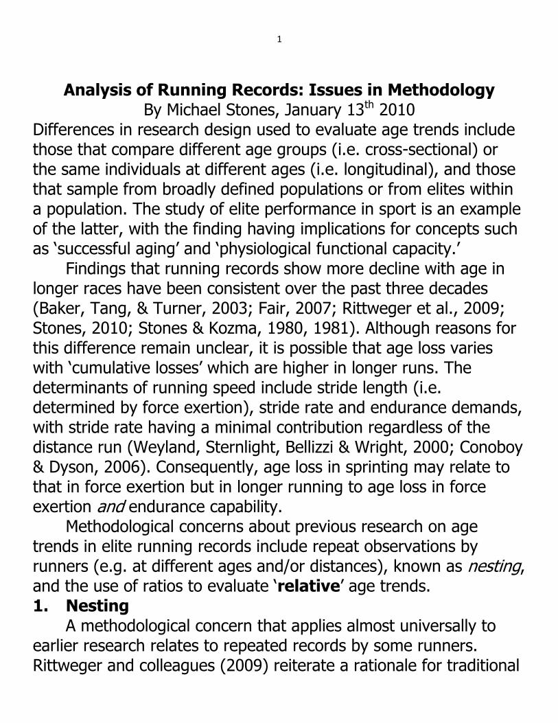
Analysis of Running Records: Issues in Methodology By Michael Stones, January 13th 2010

Differences in research design used to evaluate age trends include those that compare different age groups (i.e. cross-sectional) or the same individuals at different ages (i.e. longitudinal), and those that sample from broadly defined populations or from elites within a population. The study of elite performance in sport is an example of the latter, with the finding having implications for concepts such as „successful aging‟ and „physiological functional capacity.‟

Findings that running records show more decline with age in longer races have been consistent over the past three decades (Baker, Tang, & Turner, 2003; Fair, 2007; Rittweger et al., 2009; Stones, 2010; Stones & Kozma, 1980, 1981). Although reasons for this difference remain unclear, it is possible that age loss varies with „cumulative losses‟ which are higher in longer runs. The determinants of running speed include stride length (i.e. determined by force exertion), stride rate and endurance demands, with stride rate having a minimal contribution regardless of the distance run (Weyland, Sternlight, Bellizzi & Wright, 2000; Conoboy & Dyson, 2006). Consequently, age loss in sprinting may relate to that in force exertion but in longer running to age loss in force exertion and endurance capability.

Methodological concerns about previous research on age trends in elite running records include repeat observations by runners (e.g. at different ages and/or distances), known as nesting, and the use of ratios to evaluate „relative‟ age trends. 1. Nesting

A methodological concern that applies almost universally to earlier research relates to repeated records by some runners. Rittweger and colleagues (2009) reiterate a rationale for traditional

2

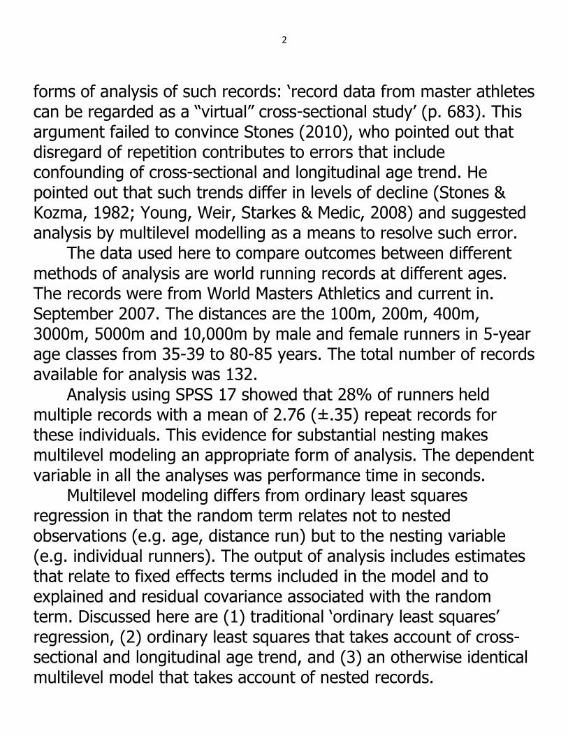
forms of analysis of such records: „record data from master athletes can be regarded as a “virtual” cross-sectional study‟ (p. 683). This argument failed to convince Stones (2010), who pointed out that disregard of repetition contributes to errors that include confounding of cross-sectional and longitudinal age trend. He pointed out that such trends differ in levels of decline (Stones & Kozma, 1982; Young, Weir, Starkes & Medic, 2008) and suggested analysis by multilevel modelling as a means to resolve such error.

The data used here to compare outcomes between different methods of analysis are world running records at different ages. The records were from World Masters Athletics and current in. September 2007. The distances are the 100m, 200m, 400m, 3000m, 5000m and 10,000m by male and female runners in 5-year age classes from 35-39 to 80-85 years. The total number of records available for analysis was 132. Analysis using SPSS 17 showed that 28% of runners held multiple records with a mean of 2.76 (±.35) repeat records for these individuals. This evidence for substantial nesting makes multilevel modeling an appropriate form of analysis. The dependent variable in all the analyses was performance time in seconds. Multilevel modeling differs from ordinary least squares regression in that the random term relates not to nested observations (e.g. age, distance run) but to the nesting variable (e.g. individual runners). The output of analysis includes estimates that relate to fixed effects terms included in the model and to explained and residual covariance associated with the random term. Discussed here are (1) traditional „ordinary least squares‟ regression, (2) ordinary least squares that takes account of cross-sectional and longitudinal age trend, and (3) an otherwise identical multilevel model that takes account of nested records.

3

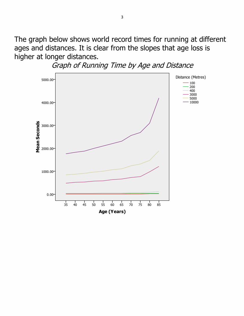
The graph below shows world record times for running at different ages and distances. It is clear from the slopes that age loss is higher at longer distances.

Graph of Running Time by Age and Distance

4

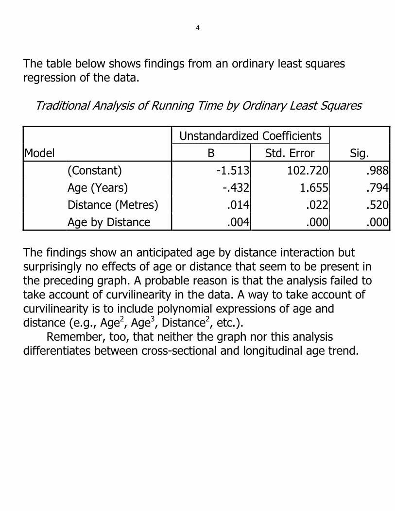
The table below shows findings from an ordinary least squares regression of the data.

Traditional Analysis of Running Time by Ordinary Least Squares

Model

Unstandardized Coefficients

Sig. B Std. Error

(Constant) -1.513 102.720 .988

Age (Years) -.432 1.655 .794

Distance (Metres) .014 .022 .520

Age by Distance .004 .000 .000

The findings show an anticipated age by distance interaction but surprisingly no effects of age or distance that seem to be present in the preceding graph. A probable reason is that the analysis failed to take account of curvilinearity in the data. A way to take account of curvilinearity is to include polynomial expressions of age and distance (e.g., Age2, Age3, Distance2, etc.).

Remember, too, that neither the graph nor this analysis differentiates between cross-sectional and longitudinal age trend.

5

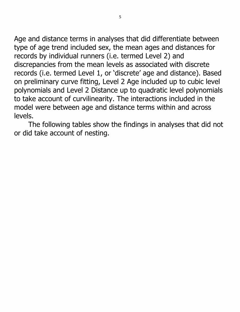
Age and distance terms in analyses that did differentiate between type of age trend included sex, the mean ages and distances for records by individual runners (i.e. termed Level 2) and discrepancies from the mean levels as associated with discrete records (i.e. termed Level 1, or „discrete‟ age and distance). Based on preliminary curve fitting, Level 2 Age included up to cubic level polynomials and Level 2 Distance up to quadratic level polynomials to take account of curvilinearity. The interactions included in the model were between age and distance terms within and across levels.

The following tables show the findings in analyses that did not or did take account of nesting.

6

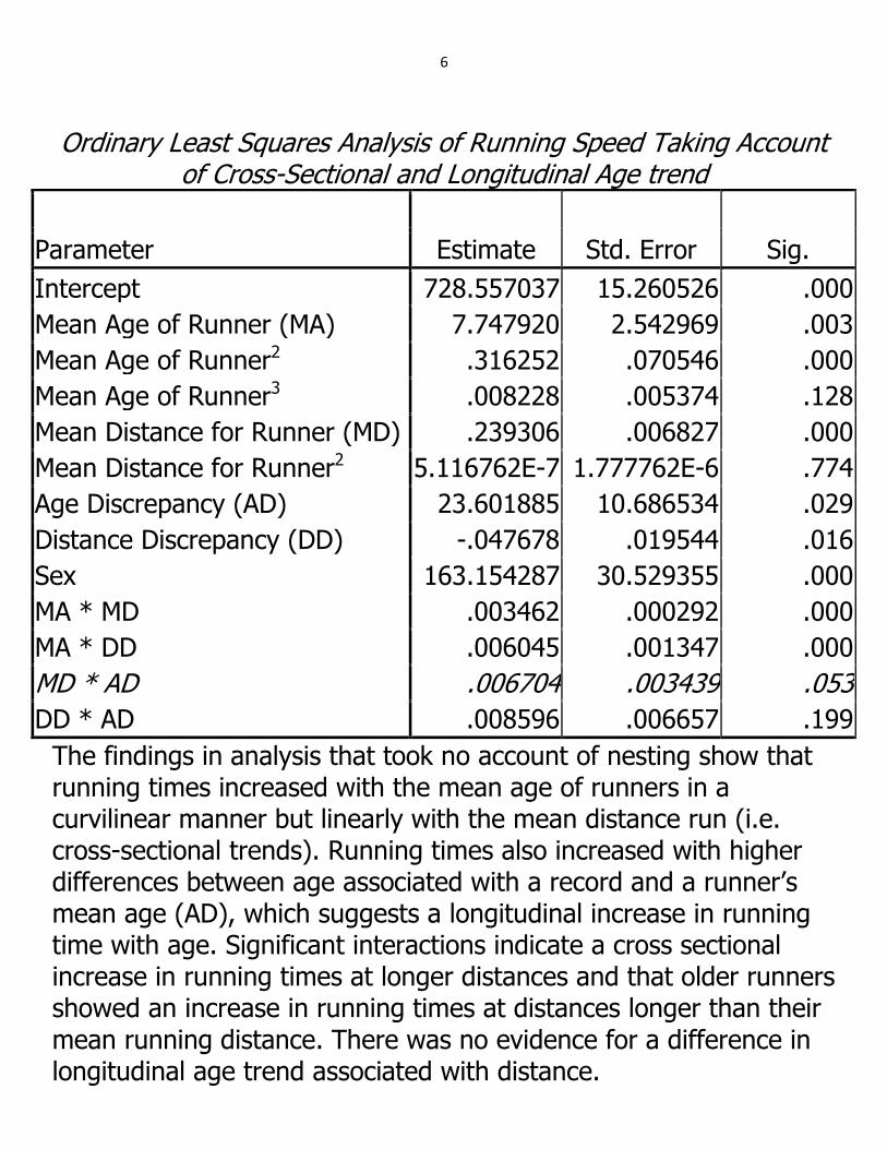
Ordinary Least Squares Analysis of Running Speed Taking Account of Cross-Sectional and Longitudinal Age trend

Parameter Estimate Std. Error Sig.

Intercept 728.557037 15.260526 .000

Mean Age of Runner (MA) 7.747920 2.542969 .003

Mean Age of Runner2 .316252 .070546 .000

Mean Age of Runner3 .008228 .005374 .128

Mean Distance for Runner (MD) .239306 .006827 .000

Mean Distance for Runner2 5.116762E-7 1.777762E-6 .774

Age Discrepancy (AD) 23.601885 10.686534 .029

Distance Discrepancy (DD) -.047678 .019544 .016

Sex 163.154287 30.529355 .000

MA * MD .003462 .000292 .000

MA * DD .006045 .001347 .000

MD * AD .006704 .003439 .053

DD * AD .008596 .006657 .199

The findings in analysis that took no account of nesting show that running times increased with the mean age of runners in a curvilinear manner but linearly with the mean distance run (i.e. cross-sectional trends). Running times also increased with higher differences between age associated with a record and a runner‟s mean age (AD), which suggests a longitudinal increase in running time with age. Significant interactions indicate a cross sectional increase in running times at longer distances and that older runners showed an increase in running times at distances longer than their mean running distance. There was no evidence for a difference in longitudinal age trend associated with distance.

7

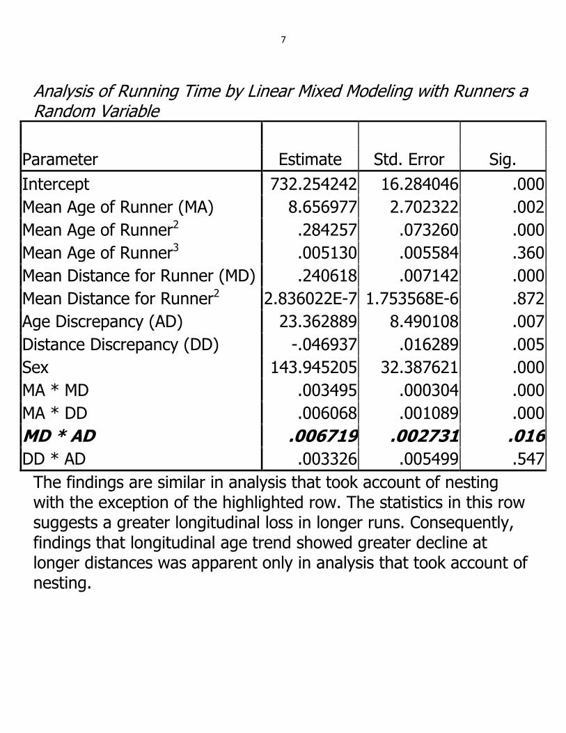
Analysis of Running Time by Linear Mixed Modeling with Runners a Random Variable

Parameter Estimate Std. Error Sig.

Intercept 732.254242 16.284046 .000

Mean Age of Runner (MA) 8.656977 2.702322 .002

Mean Age of Runner2 .284257 .073260 .000

Mean Age of Runner3 .005130 .005584 .360

Mean Distance for Runner (MD) .240618 .007142 .000

Mean Distance for Runner2 2.836022E-7 1.753568E-6 .872

Age Discrepancy (AD) 23.362889 8.490108 .007

Distance Discrepancy (DD) -.046937 .016289 .005

Sex 143.945205 32.387621 .000

MA * MD .003495 .000304 .000

MA * DD .006068 .001089 .000

MD * AD .006719 .002731 .016

DD * AD .003326 .005499 .547

The findings are similar in analysis that took account of nesting with the exception of the highlighted row. The statistics in this row suggests a greater longitudinal loss in longer runs. Consequently, findings that longitudinal age trend showed greater decline at longer distances was apparent only in analysis that took account of nesting.

8

2. „Relative’ Age Trend

Many studies of age trends in running records attempt to control for performance at the youngest age level by dividing running time at a given age by the time at the youngest age level (Baker, Tang, & Turner, 2003; Fair, 2007. The researchers refer to these ratios as „relative‟ performance.

A problem with analysis of ratios is that relationships with other variables may be spurious (i.e. nonsensical). The associated correlation may be inflated, nullified, or even inverted. Although Spearman wrote about this phenomenon of „spurious correlation‟ as long ago as 1897, researchers continue to analyze ratios despite numerous warnings in the literature about potential error.

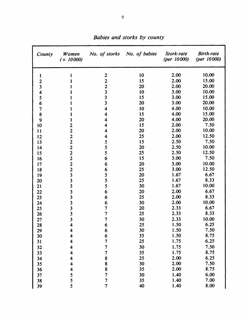
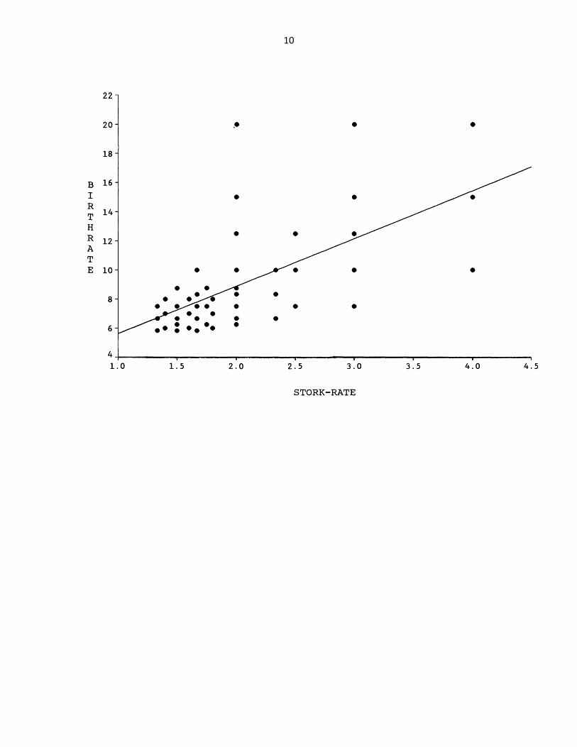
Kronmal (1993) used a fictitious example by Neyman (1952) to illustrate spurious correlation. A „friend‟ of Neyman hypothesized that the fable that storks deliver babies was true. He argued that supporting evidence would include a positive correlation between „birth rate‟ (births per 10,000 women) and „stork rate‟ (number of storks per 10,000 women) in different counties within a country. The fictitious data to test this hypothesis showed no correlation at all between number of births and number of storks (see next table). However, the correlation between birth rate and stork was .63, indicating a significant relationship illustrated by the subsequent graph.

9

10

11

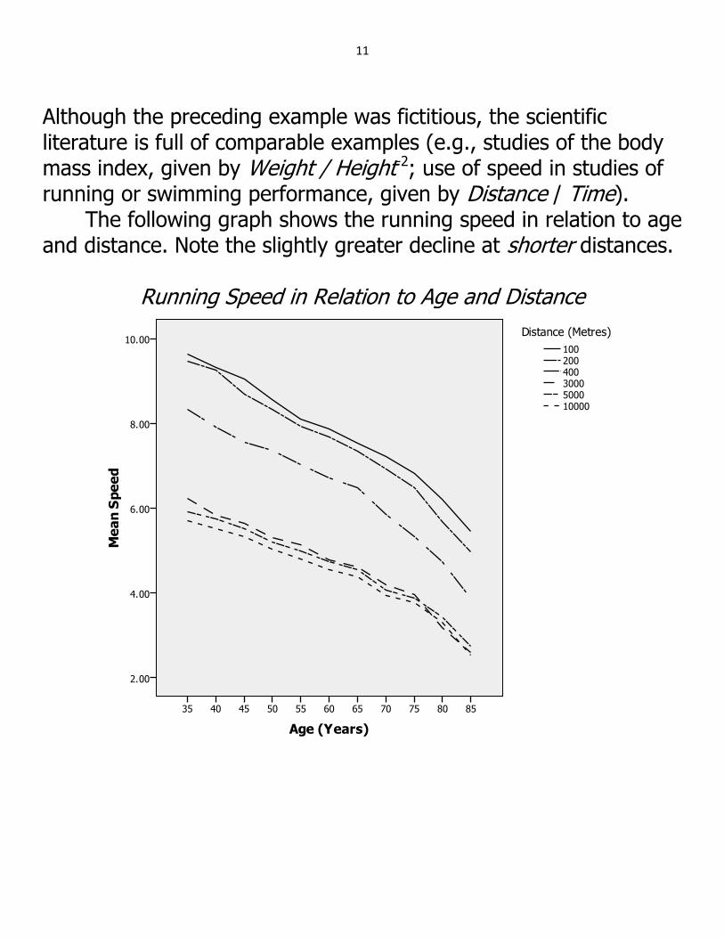
Although the preceding example was fictitious, the scientific literature is full of comparable examples (e.g., studies of the body mass index, given by Weight / Height-2; use of speed in studies of running or swimming performance, given by Distance / Time).

The following graph shows the running speed in relation to age and distance. Note the slightly greater decline at shorter distances.

Running Speed in Relation to Age and Distance

12

The very first study of age trends in freestyle swimming records used swimming speed as dependent variable and found greater loss with age at shorter distances (Hartley & Hartley, 1994). Stones and Kozma (1984) pointed out the problem with their analysis – that distance is part of both the dependent and independent variables:

Speed = α0 + α1 * Distance + α2 * Age + α3 * Distance * Age.

If we replace Speed by Distance/Time and then eliminate Distance from the left hand side of the equation through division, it is clear that what the coefficient for the interaction term (α3) represents is variation in the reciprocal of Time (i.e. 1/Time) by Age, which will be negative if swimming times are longer at older ages. Distance / Time = α0 + α1 * Distance + α2 * Age + α3 * Distance * Age, 1 / Time = α1 + α0 / Distance + α3 * Age + α2 *Age / Distance.

An appropriate linear equation to express swimming performance in relation to age and distance might take the following form: Time = α0 + α1 * Distance + α2 * Age + α3 * Distance * Age.

13

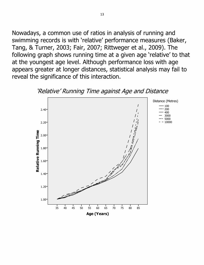
Nowadays, a common use of ratios in analysis of running and swimming records is with „relative‟ performance measures (Baker, Tang, & Turner, 2003; Fair, 2007; Rittweger et al., 2009). The following graph shows running time at a given age „relative‟ to that at the youngest age level. Although performance loss with age appears greater at longer distances, statistical analysis may fail to reveal the significance of this interaction.

„Relative‟ Running Time against Age and Distance

14

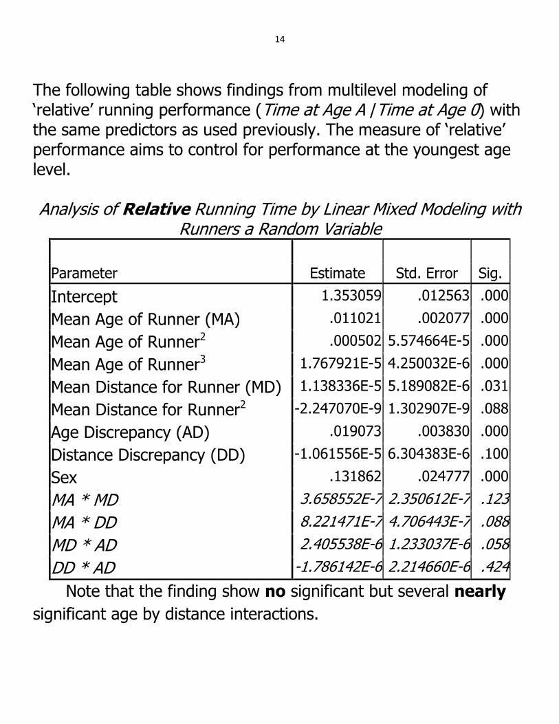
The following table shows findings from multilevel modeling of „relative‟ running performance (Time at Age A /Time at Age 0) with the same predictors as used previously. The measure of „relative‟ performance aims to control for performance at the youngest age level.

Analysis of Relative Running Time by Linear Mixed Modeling with

Runners a Random Variable

Parameter Estimate Std. Error Sig.

Intercept 1.353059 .012563 .000

Mean Age of Runner (MA) .011021 .002077 .000

Mean Age of Runner2 .000502 5.574664E-5 .000

Mean Age of Runner3 1.767921E-5 4.250032E-6 .000

Mean Distance for Runner (MD) 1.138336E-5 5.189082E-6 .031

Mean Distance for Runner2 -2.247070E-9 1.302907E-9 .088

Age Discrepancy (AD) .019073 .003830 .000

Distance Discrepancy (DD) -1.061556E-5 6.304383E-6 .100

Sex .131862 .024777 .000

MA * MD 3.658552E-7 2.350612E-7 .123

MA * DD 8.221471E-7 4.706443E-7 .088

MD * AD 2.405538E-6 1.233037E-6 .058

DD * AD -1.786142E-6 2.214660E-6 .424

Note that the finding show no significant but several nearly

significant age by distance interactions.

15

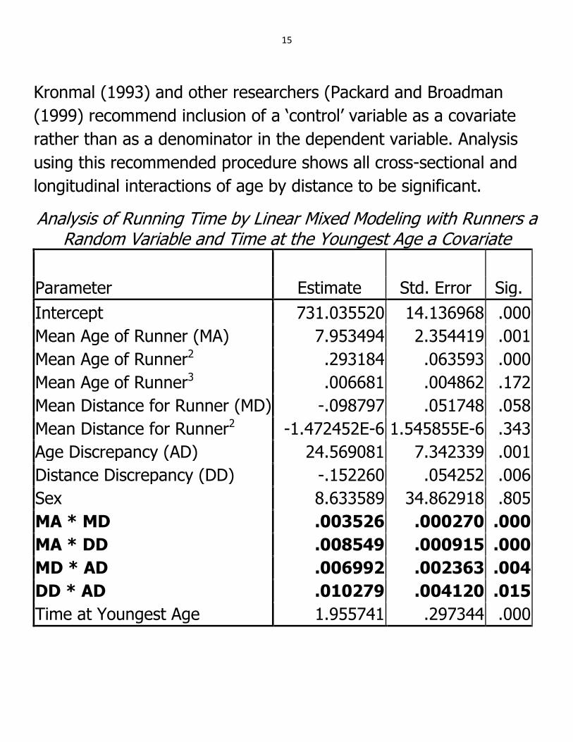
Kronmal (1993) and other researchers (Packard and Broadman

(1999) recommend inclusion of a „control‟ variable as a covariate

rather than as a denominator in the dependent variable. Analysis

using this recommended procedure shows all cross-sectional and

longitudinal interactions of age by distance to be significant.

Analysis of Running Time by Linear Mixed Modeling with Runners a Random Variable and Time at the Youngest Age a Covariate

Parameter Estimate Std. Error Sig.

Intercept 731.035520 14.136968 .000

Mean Age of Runner (MA) 7.953494 2.354419 .001

Mean Age of Runner2 .293184 .063593 .000

Mean Age of Runner3 .006681 .004862 .172

Mean Distance for Runner (MD) -.098797 .051748 .058

Mean Distance for Runner2 -1.472452E-6 1.545855E-6 .343

Age Discrepancy (AD) 24.569081 7.342339 .001

Distance Discrepancy (DD) -.152260 .054252 .006

Sex 8.633589 34.862918 .805

MA * MD .003526 .000270 .000

MA * DD .008549 .000915 .000

MD * AD .006992 .002363 .004

DD * AD .010279 .004120 .015

Time at Youngest Age 1.955741 .297344 .000

16

This presentation makes a specific case that earlier research on age trends in record running performance is replete with statistical error. Although findings with the present analyses do not overturn those from previous studies, account for nesting and control of baseline running time through regression contributed to more sensitive and accurate depiction of findings. The presentation also has relevance to a more general case that research findings are only as good as the research methodology (including the statistical procedures) used in their generation. Outside of randomized controlled designs, many studies on many topics in many disciplines fail to account for nesting that is present in the data. Also, many studies in biology, demography, economics, education, epidemiology, medicine, psychology and sociology continue to use ratio terms as dependent or independent variables. Because you should beware of findings from such studies, always examine the methodology before drawing conclusions about the accuracy of findings.