Analysis of NO3-N pollution with a distributed groundwater

Sustainability of Groundwater Resources and its Indicators (Proceedings of symposium S3 held during the Seventh IAHS Scientific Assembly at Foz do Iguaçu, Brazil, April 2005). IAHS Publ. 302, 2006.

158

Analysis of NO3-N pollution with a distributed groundwater quality model HIROAKI SOMURA1, AKIRA GOTO2, HIROYUKI MATSUI2, ELHASSAN ALI MUSA3 & MASAKAZU MIZUTANI2

1 National Institute for Rural Engineering, River and Coast Laboratory, Kan-nondai 2-1-6, Ibaraki 305-8609, Japan [email protected]

2 Faculty of Agriculture, Utsunomiya University, Minemachi 350, Tochigi 321-8505, Japan 3 Interstate Stream Commission, Santa Fe, New Mexico 87504-5102, USA

Abstract Nitrate-nitrogen (NO3-N) was selected as a groundwater resource sustainability indicator because it is well known as a cause of some diseases and the concentration in groundwater has increased gradually in recent years. We monitored it continuously from August 1996 to December 2001 in the Nasunogahara basin, Tochigi Prefecture, Japan, and constructed a distributed groundwater quality model in this basin. The model consists of two processes: infiltration of the NO3-N load into groundwater, and advection of the NO3-N load in the groundwater. As a result, the large changes of nitrogen load in the surface layer before/after heavy rainfall and the concentration changes in the groundwater by advection were well expressed. In addition, the effects of the nitrogen load infiltration from many livestock farms in the upper basin to groundwater in the lower basin were investigated. Key words alluvial fan; livestock farming; shallow aquifer; sound utilization of groundwater

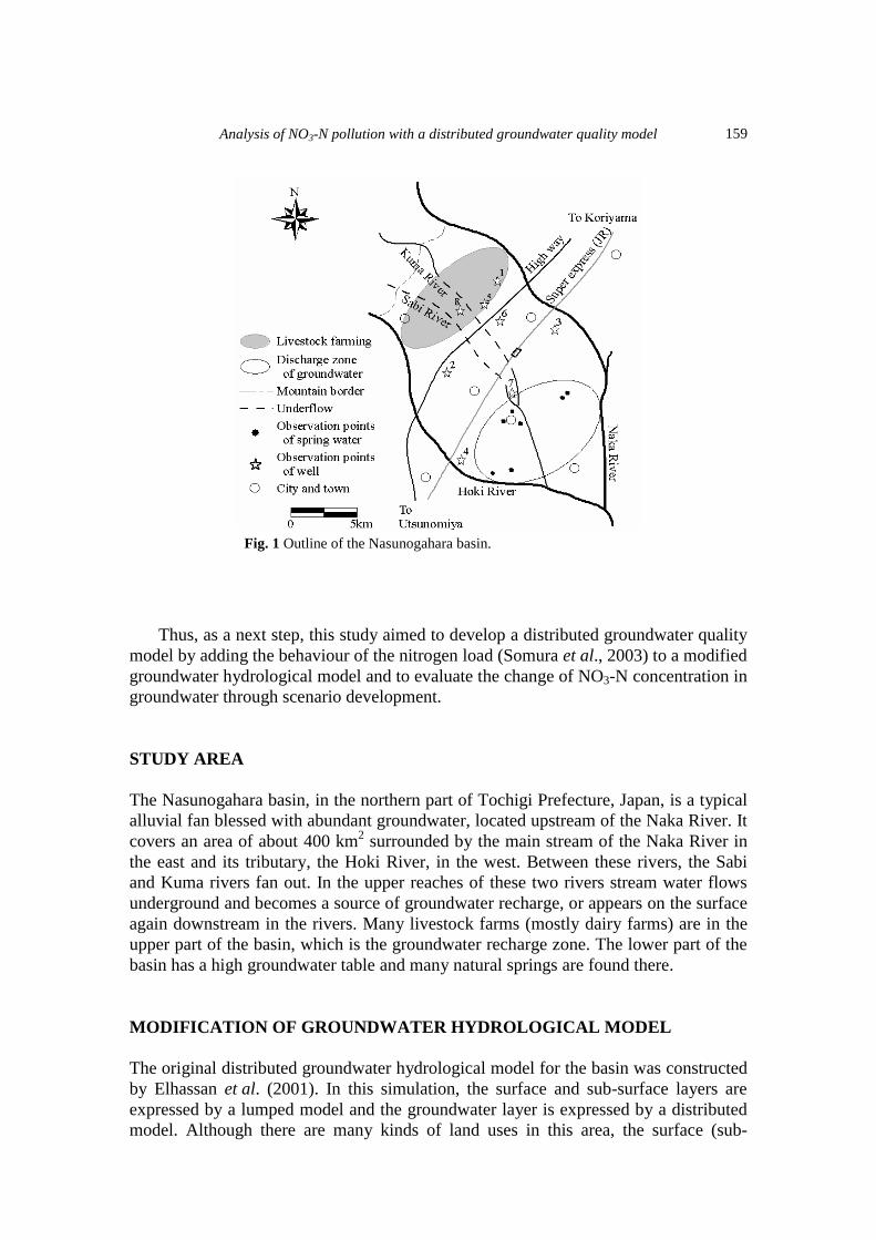
INTRODUCTION Nitrate-nitrogen (NO3-N) was selected as a groundwater resource sustainability indicator because it is well known as a cause of some diseases and the concentration in groundwater has increased gradually in recent years. One study of groundwater quality by the Environment Agency in 1982 reported that NO3-N concentration in about 10% of shallow wells in Japan exceeded 10 mg l-1, which is the environmental standard for drinking water. Generally, sewage from domestic water use, over-fertilization in upland cropping and livestock excreta are considered to be the main sources of the pollution. For the conservation and sound utilization of groundwater resources, there is a crucial need to protect groundwater from nitrogen pollution. Modelling analysis is a useful technique for examining groundwater quality. The problem of NO3-N pollution of groundwater has been recognized in the study area of the Nasunogahara basin (Fig. 1). From observations of groundwater quality in this area for several years, Somura et al. (2002) found a trend in NO3-N concentrations in shallow aquifers and the mechanism of inflow of nitrogen load to groundwater. In addition, they found that excrement from livestock farming was the most influential source of pollution. Moreover, on the basis of modelling analyses for the basin, Somura et al. (2003) expressed the inflow process of nitrogen load to unconfined aquifers by formulating such processes as storage, accumulation, dissolution and discharge, in a water quality tank model, and Elhassan et al. (2001) developed an integrated surface water—groundwater model as a distributed hydrological model.

Analysis of NO3-N pollution with a distributed groundwater quality model

159

Thus, as a next step, this study aimed to develop a distributed groundwater quality model by adding the behaviour of the nitrogen load (Somura et al., 2003) to a modified groundwater hydrological model and to evaluate the change of NO3-N concentration in groundwater through scenario development. STUDY AREA The Nasunogahara basin, in the northern part of Tochigi Prefecture, Japan, is a typical alluvial fan blessed with abundant groundwater, located upstream of the Naka River. It covers an area of about 400 km2 surrounded by the main stream of the Naka River in the east and its tributary, the Hoki River, in the west. Between these rivers, the Sabi and Kuma rivers fan out. In the upper reaches of these two rivers stream water flows underground and becomes a source of groundwater recharge, or appears on the surface again downstream in the rivers. Many livestock farms (mostly dairy farms) are in the upper part of the basin, which is the groundwater recharge zone. The lower part of the basin has a high groundwater table and many natural springs are found there. MODIFICATION OF GROUNDWATER HYDROLOGICAL MODEL The original distributed groundwater hydrological model for the basin was constructed by Elhassan et al. (2001). In this simulation, the surface and sub-surface layers are expressed by a lumped model and the groundwater layer is expressed by a distributed model. Although there are many kinds of land uses in this area, the surface (sub-

Fig. 1 Outline of the Nasunogahara basin.

Hiroaki Somura et al.

160

surface) layer was expressed by two types of land use, paddy and non-paddy. This model well represented the changes of groundwater level. Therefore, the model structure and process of water movement were applied to a distributed groundwater quality model without changes. However, from the point of view of nitrogen load transport in groundwater, water movement along the bedrock bevel might be inaccurately expressed due to use of Boussinesq’s equation (Anderson & Woessner, 1992) for the groundwater movement process. Thus, the governing equation was re-examined in order to better express nitrogen load movement in the groundwater. Governing equation in groundwater zone Generally, flow in the vertical direction can often be ignored compared to flow in the horizontal direction when considering groundwater over a wide area (JSIDRE, 2000). Thus, in this study the unconfined aquifer is assumed to be two-dimensional and flow in the vertical direction is ignored by using the assumptions of Dupuit-Forchheimer. The general flow equation for saturated groundwater flow is derived in numerous text-books. The equation is derived by mathematically combining the water balance equa-tion with Darcy’s law. The general form of the equation using Dupuit’s assumptions is:

thSyR

yhT

yxhT

x ∂∂

=+∂∂

∂∂

+∂∂

∂∂ )()( with T = k (h - b) (1)

where h is head (m); T is transmissivity (m2 s-1); R is a general source/sink term that expresses recharge and discharge (m3 s-1); Sy is the specific yield of the unconfined aquifer (the fractional volume of water that will drain freely by gravity from unit volume of the aquifer); b is the bedrock elevation (m) and t is time (second). The flows in unconfined aquifers were represented by finite difference approximation in the groundwater hydrological model. The differences of water level between time t and t + dt at node (i, j) are expressed by equation (2). The source/sink term R, which is the amount of groundwater recharge calculated by the tank model minus the amount lost from groundwater such as spring water and irrigation water, was calculated before inputting into each node:

jijijiji RAAAAthtthtSy ,4321,,, ))()()(/( ++++=−∆+∆ , with

2,,1,14

2,1,,3

2,,1,2

2,1,1,1

/))'()'((

/))'()'((

/))'()'((

/))'()'((

yththTJA

xththTJA

yththTIA

xththTJA

jijiji

jijiji

jijiji

jijiji

∆−=

∆−=

∆−=

∆−=

−−

+

+

−−

(2)

where t′ is midterm (second), TI is transmissivity in the i direction (m2 s-1) and TJ is transmissivity in the j direction (m2 s-1). Although this equation can be solved by either an implicit method or an explicit method, the implicit method was selected in this hydrological model. By replacing h(t’) with weighted average values of h(t) and h(t + dt), equation (2) can be rewritten


161

as follows, using the Crank-Nicholson scheme (θ = 0.5):

)( )()1()'( ,,, tththth jijiji ∆+θ+θ−= (3)

The Gauss-Seidel method was selected as the iteration method because it shortens the simulation time, as shown in equation (4):

))()),(),(),(()( 1,,11,,1, tthtthtthtthftth oldji

oldji

newji

newji

newji ∆+∆+∆+∆+=∆+ ++−− (4)

To further reduce the time to convergence, hi,j(t + dt) was corrected with a relaxation factor (equation (5)):

jiold

jinew

ji hREhh ,,, ∆+= (5)

where RE is the relaxation factor (0 < RE < 1). Each transmissivity TI, TJ was determined by the geometrical average of saturated zone thickness and harmonic average of hydraulic conductivity (Butler, 1957) for ease of handling the boundary condition. Simulated results of the groundwater hydrological model Simulated results were compared with data for eight wells measured by the Kanto Agricultural Bureau. The calibration period was from 1991 to 1993 and the validation period was 1994 during the simulated period. The mean absolute error (MAE), which is the mean of the absolute values of differences between measured and simulated water table elevations, was used to evaluate the goodness of fit between simulated and observed water table levels as given by:

∑=

−=n

iism WTWTnMAE

1|)(|1 (6)

where n is the number of time steps considered in the calibration and validation, WTm is the measured water table level and WTs is the simulated water table level. The MAE values for the eight wells during the calibration and validation periods are shown in Table 1. The results of the model calibration indicated good agreement Table 1 Mean absolute error (MAE) in meters for eight observation wells for calibration and validation periods.

Observation well no. Calibration period 1991–1993

Validation period 1994

Well 1 0.70 0.66 Well 2 0.68 0.38 Well 3 0.31 0.35 Well 4 0.97 0.98 Well 5 1.03 0.69 Well 6 0.96 0.75 Well 7 0.25 0.15 Well 8 2.36 2.47


162

Fig. 2 Comparison between calculated and observed water table elevations at observation well 2.

Fig. 3 Structure of the distributed groundwater quality model.

between the simulated and observed values at seven wells (except well 8), while well 8 had higher values of MAE. For the validation period, the results for most of the wells showed good agreement except for well 8. An example of observed and simulated results is shown in Fig. 2. DISTRIBUTED GROUNDWATER QUALITY MODEL Structure of the distributed groundwater quality model The distributed groundwater quality model simulated two processes: infiltration of the nitrate-nitrogen load into groundwater, and advection of the nitrate nitrogen load in the groundwater (Fig. 3). The same process proposed by Somura et al. (2003) was used for


163

Fig. 4 Migration of pollutant load in groundwater.

the infiltration process, which was expressed by two equations, the L-Q type and the dissolution type, and applied to each node in the hydrological model. It was assumed that the nitrogen load from sewage would flow directly into the unconfined aquifer. Advection process of the nitrate-nitrogen load in the groundwater The differences of the nitrate-nitrogen load between time t and t + dt at node (i, j) are expressed as zero, which is the sum of inflows and outflows by storage, advection, and diffusion. The relationship between node (i, j) and the surrounding nodes is shown in Fig. 4. Diffusion was not considered in this study because the Nasunogahara Basin has a steep slope from upstream to downstream. In order to calculate the mass inflowing to node (i, j) by advection, it is necessary to multiply velocity by the nitrate-nitrogen concentration. The concentration was approximated by the weighted mean of the concentration around the node. Since only advection was considered in this study, the weighted mean was calculated by the upwind method (Kinzelbach, 1986). The load transport between node (i, j) and the surrounding nodes (i – 1, j) (i + 1, j) (i, j – 1) (i, j + 1) was calculated by equation (7):

2/)())1((2/)())1((

2/)())1((2/)())1((

1,,1,4,4,4

,1,,31,31,3

,1,,12,2,2

,,1,1,11,11

tSymmyCwgtCwgtuxLtSymmyCwgtCwgtuxL

tSymmxCwgtCwgtuyLtSymmxCwgtCwgtuyL

jijijijiji

jijijijiji

jijijijiji

jijijijiji

∆+∆−+=

∆+∆−+=

∆+∆−+=

∆+∆−+=

++

−−−

++

−−−

(7)

Thus, the load balance derived by advection was expressed by equation (8):

(Lc) i, j = L1 – L2 +L3 – L4 (8)

where ux, uy is the velocity between two nodes (m s-1), C is the concentration (mg L-1), m is the thickness of the saturated zone (m), Lc is the variation of the load (kg), and


164

wgt1, wgt2, wgt3, wgt4 are weights, which were calculated by:

2/))(sign1(2/))(sign1(

2/))(sign1(2/))(sign1(

,4

1,3

,2

,11

ji

ji

ji

ji

uxwgtuxwgtuywgtuywgt

+=

+=

+=

+=

−

−

with

<−=>+

=0 0 00

)(signaaa

a (9)

The velocity between two nodes was determined by the calculated heads at the nodes. The Darcy velocity between two nodes was calculated from the difference of the head as shown in equation (10):

yhhjikvyxhhjikvx

jijiyji

jijixji

∆−−=

∆−−=

+

+

/))(,(/))(,(

,,1,

,1,, (10)

Moreover, the velocities ux, uy were determined by dividing the Darcy velocity by the specific yield as shown in equation (11):

SyvyuySyvxux

jiji

jiji

//

,,

,,

=

= (11)

where vx, vy are the Darcy velocity between two nodes (m s-1), kx(i, j) is the hydraulic conductivity between nodes (i, j) and (i, j + 1), and ky(i, j) is the hydraulic conductivity between nodes (i, j) and (i + 1, j). Calculation of the nitrate-nitrogen concentration To calculate the concentration at a node (i, j), it was necessary to estimate the load storage at node (i, j) from the difference of inflow and outflow. As the load variation by advection was calculated by equation (8), loads in percolation and discharge were derived as follows. The sum of the load inflow to groundwater was determined from the loads in percolation calculated for both the paddy and non-paddy tanks as follows:

(Lperco) i, j = (Lpaddy) i, j + (Lnonpaddy) i, j (12)

where Lperco is the sum of the percolation load from the tank (kg), Lpaddy is the percolation load from the paddy tank (kg), and Lnonpaddy is the percolation load from the non-paddy tank (kg). The load in discharge water from groundwater was calculated as shown in equation (13):

(Ldischarge) i, j = (Lspring) i, j + (Lpump) i, j (13)

with

(Lspring) i, j = (Sdischarge) i, j × ∆x∆y × C i, j

(Lpump) i, j = (Pdischarge) i, j × ∆x∆y × C i, j


165

where Ldischarge is the sum of the discharge load from the groundwater (kg), Lspring is the load in spring water (kg), Lpump is the load in irrigation water pumped up from the groundwater, Sdischarge is the height of the spring water discharge (m), and Pdischarge is the height of the irrigation water pumped up from the groundwater (m). In this study, the loads in spring water and irrigation water from the groundwater were considered as discharge load from the groundwater. The load storage at node (i, j) was determined by equations (8), (12), (13), and the load in sewage by equation (14):

(Lbalance) i, j = (LC) i, j + (Lperco) i, j – (Ldischarge) i, j + swg i, j (14)

where Lbalance is the load storage at node (i, j) (kg) and swg is the load in sewage (kg). The concentration at node (i, j) was calculated by the load storage at node (i, j) and water storage at node (i, j) as follows:

C i, j = (Lbalance) i, j / (m i, j ×Sy × ∆x × ∆y) (15)

where C is the concentration at node (i, j). Evaluation of simulated NO3-N concentrations Simulated NO3-N concentrations were compared with data from five spring water monitoring points. The calibration period was from 1996 to 2000 and the validation period was 2001 during the simulated period. The average relative error (ARE), which is the average of the relative values of differences between measured and simulated NO3-N concentrations, was used to evaluate the goodness of fit between simulated and observed concentration as follows:

∑=

−=n

iimsm CCCnARE

1|)/)((|1 (16)

where Cm is the measured concentration of NO3-N and Cs is the simulated concentra-tion of NO3-N. Table 2 Other input data.

Jan. Feb. Mar. Apr. May June July Aug. Sep. Oct. Nov. Dec. Fertilizer and manure (kg km-2 day-1)

paddy tank non-paddy tanks

0 5

0 9

0 31

301 71

0 51

0 69

81 3

65 10

0 8

27 10

0 31

0 0

Plant uptake (kg km-2 day-1)


1 1

8 7

17 15

15 16

33 26

81 35

81 36

60 35

32 23

11 17

5 4

1 1

Denitrification and volatization (kg km-2 day-1)


4 4

4 4

4 4

18 4

18 4

18 4

18 4

18 4

18 4

4 4

4 4

4 4


166

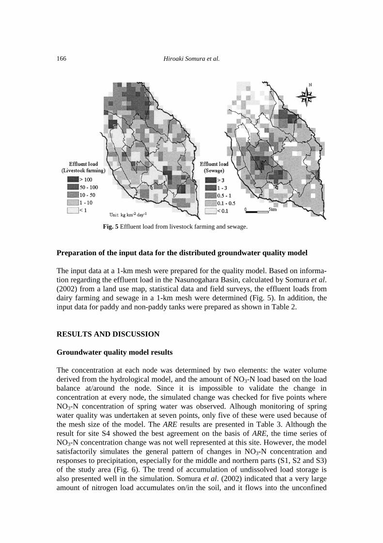
Fig. 5 Effluent load from livestock farming and sewage.

Preparation of the input data for the distributed groundwater quality model The input data at a 1-km mesh were prepared for the quality model. Based on informa-tion regarding the effluent load in the Nasunogahara Basin, calculated by Somura et al. (2002) from a land use map, statistical data and field surveys, the effluent loads from dairy farming and sewage in a 1-km mesh were determined (Fig. 5). In addition, the input data for paddy and non-paddy tanks were prepared as shown in Table 2. RESULTS AND DISCUSSION Groundwater quality model results The concentration at each node was determined by two elements: the water volume derived from the hydrological model, and the amount of NO3-N load based on the load balance at/around the node. Since it is impossible to validate the change in concentration at every node, the simulated change was checked for five points where NO3-N concentration of spring water was observed. Alhough monitoring of spring water quality was undertaken at seven points, only five of these were used because of the mesh size of the model. The ARE results are presented in Table 3. Although the result for site S4 showed the best agreement on the basis of ARE, the time series of NO3-N concentration change was not well represented at this site. However, the model satisfactorily simulates the general pattern of changes in NO3-N concentration and responses to precipitation, especially for the middle and northern parts (S1, S2 and S3) of the study area (Fig. 6). The trend of accumulation of undissolved load storage is also presented well in the simulation. Somura et al. (2002) indicated that a very large amount of nitrogen load accumulates on/in the soil, and it flows into the unconfined


167

aquifer together with rain water infiltration. In addition, heavy storms may flush out the nitrogen load in the soil and reduce accumulation to a low level (Fig. 6). The simu-lations also suggest spatial variability in concentration and load behaviour within the basin. For example, modelled changes in load before/after heavy rain in 1998 (Fig. 7) reveal a sudden decrease of the load with rain water infiltration in the basin, and a dra-matic change in the amount of load in the upper part of the basin, as well as a change in concentration caused by advection from the upper to the lower basin. In contrast, simulations for a dry period extending for more than 10 days, reveal only slow change in the distribution of concentrations in the upper and lower basins (Fig. 8). Table 3 Average relative error (ARE) with simulated and observed spring water.

Spring water NO Calibration period 1996–2000 Validation period 2001 S1 41.9 30.5 S2 36.9 25.2 S3 39.2 28.0 S4 23.3 11.1 S5 34.9 49.8

Fig. 6 Simulated result of water quality (a) and change in load storage (b).

( )

(

a

)
b


168

Fig. 7 Change in load storage in soil before/after heavy rain.

Fig. 8 Change in NO3-N concentration of groundwater during period of no rainfall.

Because the model was regarded as providing reasonable simulations of NO3-N concentrations in space and time, it was used in conjunction with a number of scenarios to determine the impacts of effluent load control and land use change on groundwater concentrations.


169

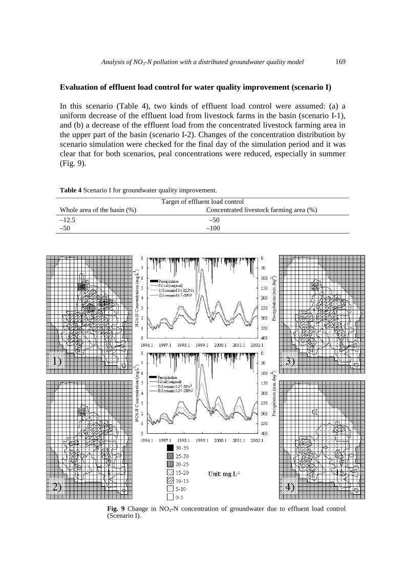
Evaluation of effluent load control for water quality improvement (scenario I) In this scenario (Table 4), two kinds of effluent load control were assumed: (a) a uniform decrease of the effluent load from livestock farms in the basin (scenario I-1), and (b) a decrease of the effluent load from the concentrated livestock farming area in the upper part of the basin (scenario I-2). Changes of the concentration distribution by scenario simulation were checked for the final day of the simulation period and it was clear that for both scenarios, peal concentrations were reduced, especially in summer (Fig. 9). Table 4 Scenario I for groundwater quality improvement.

Target of effluent load control Whole area of the basin (%) Concentrated livestock farming area (%) –12.5 –50 –50 –100

F

(
ig. 9 Change in NO3-N concentration of groundwater due to effluent load control
Scenario I).


170

Effect of the decrease in the area of paddy fields (scenario II) In recent years, commuter towns have sprung up in this basin and the population is in-creasing gradually. In addition, the area of paddy field cultivation has decreased under a policy of reducing rice acreage in Japan. Thus, paddy fields will become housing sites and the hydrological environment in the basin will change in the future. The effect of the decrease in the area of paddy fields in the basin was examined in this scenario with a decline by 10, 30 and 50% being studied.. Changes of the concentra-tion distribution by scenario simulation were checked for the final day of the simula-tion period, but large changes in the spatial distribution of groundwater concentrations were not recognized spatially, although an increase in concentration was observed as paddy field area decreased (Fig. 10).

Discussion of improvement of groundwater concentration through scenario analysis As the graphs for scenario I-1 (Fig. 9, parts 1 and 2) reveal, controlling the effluent load from livestock farms in the basin affects the peak concentration in groundwater, especially in summer. Rainfall is high during summer in Japan, so reducing the load on/in the soil by reducing the effluent load would decrease the load caused by rain water infiltration into groundwater. However, as it is very difficult to reduce the efflu-ent load in the whole basin uniformly, scenario I-2 is more viable for the study area. As shown in Fig. 9 (parts 3 and 4), decreasing the effluent load from the concentrated livestock farming area has a large effect in the middle and northern part of the basin. The concentration in the middle part of the basin became low when the reduction ratio was 100%. Also, reducing the effluent load from the concentrated livestock farming area improved the concentration in the groundwater overall. Thus, targeting the

Fig. 10 Effect of paddy field decrease on groundwater quality.


171

construction of composting facilities to reduce the effluent load from the concentrated livestock farming area in the upper part of the basin would be a good strategy to improve groundwater quality, especially in the lower part of the basin. Changes in the area of paddy field concentration may affect groundwater concentrations through alteration in water movement, but this impact would be very small compared with the effect of reducing effluent loads from livestock. CONCLUSIONS A distributed groundwater quality model was constructed by adding the behaviour of the nitrogen load to a groundwater hydrological model. This model simulated the change in NO3-N concentration of the groundwater by advection and revealed regional differences of concentration based on the spatial distribution of effluent load. Simulation on the basis of different scenarios suggested the amount of influent load from the concentrated livestock farming area has a considerable impact on the concentration in the groundwater in the northern and middle part, while a change of water movement and amount of effluent load associated with a decrease in area of paddy fields would affect peak NO3-N concentration, especially in summer. REFERENCES Anderson, M. P. and Woessner, W. W. (1992) Applied Groundwater Modelling: Simulation of Flow and Advective

Transport. Academic Press, San Diego, California, USA. Butler, S. S. (1957) Engineering Hydrology. Prentice Hall, Englewood Cliffs, New Jersey, USA. Elhassan, A. M., Goto, A. & Mizutani, M. (2001) Combining a tank model with a groundwater model for simulating

regional groundwater flow in an alluvial fan. Trans. of the JSIDRE, 69(5), 583–591. JSIDRE (2000) Handbook of Agricultural Engineering, 6th edn. Basic volume (Nogyo Doboku Handbook), 66–73 (in

Japanese). Kinzelbach, W. (1986) Groundwater modelling: an introduction with sample programs in Basic. In: Developments in

Water Science, Vol. 25. Elsevier Science Publishers BV, Amsterdam, The Netherlands. Somura, H., Masuda, M., Goto, A. & Mizutani, M. (2002) Groundwater nitrogen pollution and its mechanism in

Nasunogahara Basin, Tochigi Pref., Japan. Trans. of the JSIDRE, 70(3), 365–373 (in Japanese). Somura, H., Goto, A. & Mizutani, M. (2003) Modelling Analysis of nitrate nitrogen pollution processes of groundwater in

Nasunogahara Basin. Trans. of the JSIDRE, 71(4), 455–464.

Documents

Analysis of NO3-N pollution with a distributed groundwater