Embed Size (px)
Citation preview
Contents lists available at ScienceDirect
Journal of the Mechanics and Physics of Solids
Journal of the Mechanics and Physics of Solids ∎ (∎∎∎∎) ∎∎∎–∎∎∎
http://d0022-50
n CorrE-m
PleasPhys
journal homepage: www.elsevier.com/locate/jmps
Analysis of necking based on a one-dimensional model
Basile Audoly a,b,n, John W. Hutchinson c
a Sorbonne Universités, UPMC Univ Paris 06, UMR 7190, Institut Jean Le Rond d'Alembert, F-75005 Paris, Franceb CNRS, UMR 7190, Institut Jean Le Rond d'Alembert, F-75005 Paris, Francec School of Engineering and Applied Sciences, Harvard University, Cambridge, MA 02138, USA
a r t i c l e i n f o
Article history:Received 9 February 2015Received in revised form17 October 2015Accepted 21 December 2015
Keywords:Beams and columnsElastic-plastic materialStability and bifurcationAsymptotic analysis
x.doi.org/10.1016/j.jmps.2015.12.01896/& 2015 Elsevier Ltd. All rights reserved.
esponding author at: Sorbonne Universités,ail address: [email protected]. (B. Audo
e cite this article as: Audoly, B., Hu. Solids (2016), http://dx.doi.org/10.
a b s t r a c t
Dimensional reduction is applied to derive a one-dimensional energy functional govern-ing tensile necking localization in a family of initially uniform prismatic solids, includingas particular cases rectilinear blocks in plane strain and cylindrical bars undergoing ax-isymmetric deformations. The energy functional depends on both the axial stretch and itsgradient. The coefficient of the gradient term is derived in an exact and general form. Theone-dimensional model is used to analyze necking localization for nonlinear elastic ma-terials that experience a maximum load under tensile loading, and for a class of nonlinearmaterials that mimic elastic-plastic materials by displaying a linear incremental responsewhen stretch switches from increasing to decreasing. Bifurcation predictions for the onsetof necking from the simplified theory compared with exact results suggest the approach ishighly accurate at least when the departures from uniformity are not too large. Post-bi-furcation behavior is analyzed to the point where the neck is fully developed and localizedto a region on the order of the thickness of the block or bar. Applications to the nonlinearelastic and elastic-plastic materials reveal the highly unstable nature of necking for theformer and the stable behavior for the latter, except for geometries where the length ofthe block or bar is very large compared to its thickness. A formula for the effective stressreduction at the center of a neck is established based on the one-dimensional model,which is similar to that suggested by Bridgman (1952).
& 2015 Elsevier Ltd. All rights reserved.
1. Introduction with précis of the dimensional reduction
The tension test is one of the canonical methods to measure the stress–strain behavior of materials. A well-knowncomplication for ductile materials which undergo a maximum load in the test is necking wherein deformation localizes in aregion on the order of the specimen thickness at some location along the length of the specimen. Considère (1885) de-scribed the connection of the onset of the localization process to the maximum load, and the criteria for the stress and strainat the onset of necking bear his name. Since Considère's time, necking has received a great deal of attention in the scientificand engineering literatures not only because of its importance in measuring material properties (Bridgman, 1952) butbecause it is often a precursor to material failure (Marciniak and Kuczyński, 1967). Necking phenomena are highly nonlinearowing to both material and geometric nonlinearities. Detailed fully nonlinear analyses of necking emerged in the early1970's after finite strain plasticity formulations were developed and computers became available with the capacity to carry
UPMC Univ Paris 06, UMR 7190, Institut Jean Le Rond d'Alembert, F-75005 Paris, France.ly).
tchinson, J.W., Analysis of necking based on a one-dimensional model. J. Mech.1016/j.jmps.2015.12.018i
B. Audoly, J.W. Hutchinson / J. Mech. Phys. Solids ∎ (∎∎∎∎) ∎∎∎–∎∎∎2
out the requisite computations. Chen's (1971) Galerkin-like approach to necking in bars was soon followed by finite elementanalyses of necking in round bars by Needleman (1972) and Norris et al. (1978). These and subsequent studies provided theneck shape and the stress and strain distributions within the neck for cross-sections that had localized to less than one halfof the cross-sectional area outside of the neck.
During this same period, analytical conditions for the onset of necking were derived within the framework of Hill's(1961) bifurcation theory for elastic-plastic solids: both the cases of a cylinder having a circular cross-section (Hutchinsonand Miles, 1974) and of a 2D rectangular block in plane strain (Hill and Hutchinson, 1975) were considered. These analyseswere later extended in two ways: Scherzinger and Triantafyllidis (1998) considered the linear stability of general prismaticsolids (with non-circular cross-section), Triantafyllidis et al. (2007) addressed the post-bifurcation problem by means of aLyapunov–Schmidt–Koiter expansion for a 2D rectangular block for various constitutive laws. In line with these local sta-bility results, Sivaloganathan and Spector (2011) showed that the homogeneous solution is, in a global sense, the onlyabsolute minimizer of the energy for a class of constitutive behaviors such that the load/displacement curve does notpossess a maximum. The latter approach tells nothing about the necking instability; the other 2D or 3D approaches arelimited to the linear or weakly non-linear analysis of necking.
Approximate 1D models offer an appealing alternative to 2D and 3D approaches, making it possible to analyze theessential nonlinear aspects of necking. Ericksen (1975) notes that simple bar models, whereby the density of stored elasticenergy is a function of the centerline stretch only, give rise to discontinuous solutions past the point of maximum load. Aregularized elastic energy functional is therefore needed, which is typically assumed to depend on the gradient of thecenterline stretch as well. Based on regularized models of this kind, Antman (1973) carries out a linear bifurcation analysis,Antman and Carbone (1977) address the initial post-bifurcation behavior; Coleman and Newman (1988) construct non-linear solutions exhibiting localized necks, while Owen (1987) discusses their stability.
With the exception of the work of Mielke, discussed below, one-dimensional models used for the analysis of necking arenot derived from 2D or 3D continuum mechanics by proper dimensional reduction. The model of Owen (1987), for instance,is based on a kinematical assumption for the shear which is not applicable in the slender limit, as noted by Mielke (1991);the dimensional reduction of Coleman and Newman (1988) is based on a similar assumption and we discuss it later in detail.To the best of our knowledge, the dimensional reduction of Mielke (1991), which uses the central manifold theorem, is theonly one which is asymptotically exact, i.e. it predicts not only the form of the regularized energy functional but also thecorrect value of its coefficients. Mielke's analysis is done for a 2D rectangular block made of a hyperelastic material. Here, weextend his work in the following ways: we consider 3D prismatic solids having an arbitrary cross-section and made of anorthotropic material, and we recover the case of a 2D block made of an isotropic material as a special case; we also derive asimple formula for the modulus associated with the regularizing second-gradient term, which captures the dependence onboth the cross-sectional geometry and on the constitutive law; finally, we extend the 1D model to account for the elasticunloading of elastic/plastic materials.
The analytical details of the dimensional reduction leading to the one-dimensional necking model are presented inSection 2 for a family of uniform prismatic solids. The final mathematical model is simple even though the reduction itself issomewhat technical. Thus, a summary of the equations governing the 1D model is included in this Introduction, see below:this allows the reader to skip Section 2 and proceed directly to the applications covered in Sections 3 and 4. In Section 3, the1D model is used to characterize the response of a nonlinear elastic material whose loading curve displays a maximum load.In Section 4, we extend the model to account for the elastic unloading of an elastic/plastic material, and show that thisspecific unloading response can completely modify the global necking behavior. It should be emphasized that the 1D re-duction is not meant to capture the transition from necking to shear localization, nor the shear localization itself, whichoften occurs in the advanced stages of necking in of metal bars or sheets.
The general derivation in Section 2 considers prismatic solids having an arbitrary cross-section and takes into account
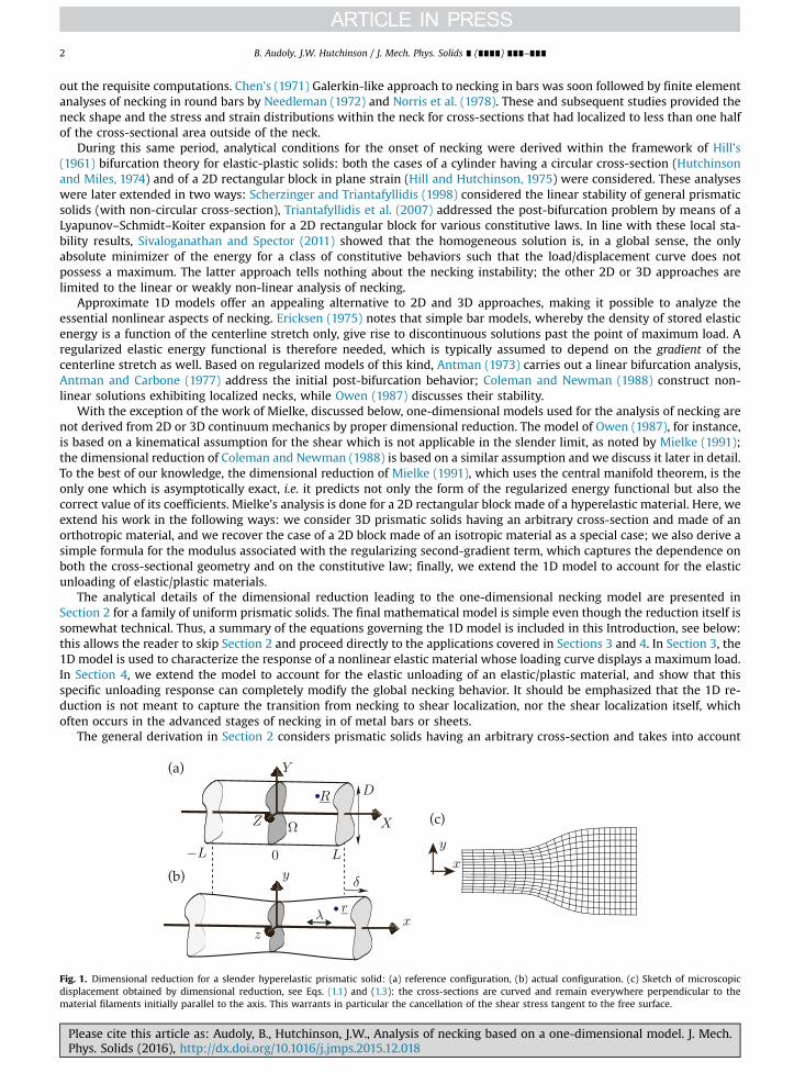
Fig. 1. Dimensional reduction for a slender hyperelastic prismatic solid: (a) reference configuration, (b) actual configuration. (c) Sketch of microscopicdisplacement obtained by dimensional reduction, see Eqs. (1.1) and (1.3): the cross-sections are curved and remain everywhere perpendicular to thematerial filaments initially parallel to the axis. This warrants in particular the cancellation of the shear stress tangent to the free surface.
Please cite this article as: Audoly, B., Hutchinson, J.W., Analysis of necking based on a one-dimensional model. J. Mech.Phys. Solids (2016), http://dx.doi.org/10.1016/j.jmps.2015.12.018i
B. Audoly, J.W. Hutchinson / J. Mech. Phys. Solids ∎ (∎∎∎∎) ∎∎∎–∎∎∎ 3
orthotropy and material compressibility, but in this section and in the applications attention is limited to 2D blocks orcircular cylinders (round bars) and to isotropic nonlinear elastic materials that are incompressible. The geometry in theundeformed and deformed states is indicated in Fig. 1, including notation used throughout the paper. In the undeformedstate, the block is rectangular with thickness h and length 2L in 2D, and the round bar in 3D is uniform with a cross-sectiondiameter D and length 2L. The coordinate X identifies material cross-sections in the undeformed state. In the deformed state,the cross-sections become curved and the coordinate of their average axial position is denoted by Λ= ( )x X . The stretch isthen defined as λ ( ) = ΛX
Xdd; it characterizes the deformation state of the block or bar in the one-dimensional reduction. The
lateral faces of the block (or the lateral surface of the bar) are traction-free. Particular attention will be given to solutionsthat are symmetric with respect to the point X¼x¼0, which is assumed to lie at the center of the neck. Idealized conditionsare applied on the endpoints, namely symmetry conditions at X¼0, and the condition of zero shear tractions at X¼L. Theseboundary conditions admit the uniform stretch, λ δ= + L1 /0 as one solution for an initially perfect block or bar, where δ isthe elongation of the right-hand side half of the specimen.
For non-uniform stretching the dimensional reduction in Section 2 starts by observing that a non-homogeneous con-figuration having planar cross-sections is close to (but not exactly at) equilibrium, and seeks an equilibrium solution by aperturbation method. This approach works under the assumption that the prescribed inhomogeneous stretch λ ( )X varies ona much longer length-scale than the cross-section dimension h or D: a linearized elasticity problem with small residualstrain yields the sought equilibrium solution, which has curved cross-sections. The primary independent variable in theone-dimensional theory is the macroscopic stretch measure, λ ( )X , and the dimensional reduction assigns an energy to anyprescribed stretch distribution λ ( )X .
We stress that the dimensional reduction does not start by linearizing near a uniform solution with constant stretchλ λ( ) =X 0—if that were the case, its validity would be limited to configurations such that λ ( )X stays uniformly close to aconstant value λ0. Instead, we linearize near a non-equilibrium configuration having a slowly varying stretch λ ( )X —for aslender block or bar, the stretch λ ( )X may well vary significantly over the entire length. This feature is particularly desirablein the context of necking, where the relevant solutions are slowly variable, but far from homogeneous as a whole.
First, consider the block in plane strain, with thickness h and out-of-plane stretch λ = 1II . With the largest principal stretchas λI and the minimum principal stretch as λ λ= 1/III I , the material is characterized microscopically by an energy densityfunction λ( )w I0 . The Cauchy (true) stress for a block that undergoes uniform stretch λ λ δ= = + L1 /I0 isσ σ λ λ λ≡ ( ) = ( )
λw
11 0 0 0dd 0
0 , while the nominal, or engineering stress, is λ λ( ) = ( )λ
n w0 0
dd 0
0 . The analysis in Section 2 provides thefollowing result for the location of a material point in the deformed state (x,y) in terms of its location in the undeformedstate (X,Y):
⎛⎝⎜
⎞⎠⎟Λ
λλ
λ= ( ) +
( )− =
( )x X
X XY
hy Y
12
dd 12
and1
.1.14
22
Here, ∫Λ λ( ) = ( ′) ′X X XdX
0denotes the mapping from the coordinate X of a cross-section in reference configuration, to its
average coordinate Λ ( )X in deformed configuration. The quantity λ ( )X , defined as the derivative of Λ ( )X , is also the cross-sectional average of the axial deformation gradient: we shall refer to it as the macroscopic stretch, or simply the stretch. ByEq. (1.1), λ ( )X is also the axial stretch of the two material filaments with equation = ± ( )Y h/ 2 3 , initially parallel to the axis.The strain energy in the block (per unit depth out-of-plane) associated with this approximation is
⎡⎣⎢⎢
⎛⎝⎜
⎞⎠⎟
⎤⎦⎥⎥∫ λ λ λ λ λ
λ= ( ) + ( ) ( ) = ( ) ( )
( )W h w
hb
XX b
n2
dd
d with12
incompressible 2D block .1.2
L
00
2 20
5
The second term in the integrand depends on the second gradient of displacement, the stretch λ being its first gradient. Inthe modulus b associated with this second-gradient term, note that the engineering stress for the homogeneous solutions
λ( ) =λ
n w0
dd
0 is evaluated with the local value of the stretch λ λ= ( )X . As a result, any nonlinearity present in the original 3Dconstitutive law is accurately captured in the 1D energyW: this warrants the accuracy of the model into the nonlinear range.
The corresponding results for the round bar undergoing axisymmetric deformation are also expressed in terms of thestretch λ ( )X . Denote the strain energy density for an isotropic incompressible elastic material under uniaxial stretch states(with principal stretches λI and λ λ μ λ= = = −
II III I1/2) by λ( )w I0 . The true axial stresses under a uniform stretch, λ0 = λI is now
σ λ λ λ( ) = ( )λ
w0 0 0
2 dd 0
0 , while the nominal stress is unchanged, λ λ( ) = ( )λ
n w0 0
dd 0
0 . Let R denote the radial distance of a materialpoint from the centerline in the undeformed state and r denote this distance in the deformed state. In the one-dimensionapproximation, the location of a material point (x,r) in the deformed state in terms of (X,R) is
⎛⎝⎜
⎞⎠⎟Λ
λλ
λ= ( ) +
( )− =
( )x X
X XR
Dr R
14
dd 8
and1
,1.33
22
with D as the diameter of the undeformed bar. The macroscopic stretch λ ( )X is still the cross-sectional average of the axialdeformation gradient; for a round bar, it also matches the microscopic stretch of the filaments initially located at a distance
= ( )R D/ 2 2 from the axis, see the equation above. The energy in the bar is
Please cite this article as: Audoly, B., Hutchinson, J.W., Analysis of necking based on a one-dimensional model. J. Mech.Phys. Solids (2016), http://dx.doi.org/10.1016/j.jmps.2015.12.018i
B. Audoly, J.W. Hutchinson / J. Mech. Phys. Solids ∎ (∎∎∎∎) ∎∎∎–∎∎∎4
⎛⎝⎜
⎞⎠⎟
⎡⎣⎢⎢
⎛⎝⎜
⎞⎠⎟
⎤⎦⎥⎥∫π λ λ λ λ λ
λ= ( ) + ( ) ( ) = ( ) ( )
( )W
Dw
Db
XX b
n4 2
dd
d with32
incompr. circular cyl. .1.4
L2
00
2 20
4
2. Dimensional reduction
The goal of this section is to establish by means of asymptotic expansions the second-gradient bar model outlined above,which describes the onset and development of localization in a prismatic beam. We work with an hyperelastic materialwhich is orthotropic and has its material symmetry axis aligned with the axis of the prismatic domain (note that hisincludes isotropic materials as a particular case). The material is assumed compressible; the incompressible limit will beworked out at the end as a special case. The cross-section geometry is arbitrary as well for the moment: the case of a roundbar, or of a 2D block will also be worked out as a special case at the end, see Section 2.9. The entire Section 2 can be skippedas it is independent of the rest of the paper, except for the final expressions of the second-gradient model which aresummarized in Section 2.8. The models applicable to the special cases of a 2D block or a round bar made of an in-compressible material have been announced at the end of the Introduction.
2.1. Geometry: a prismatic solid
We consider an elastic body whose reference configuration is a prism of length 2 L, having a typical cross-sectionaldiameter D, see Fig. 1. We assume that the slenderness parameter ϵ = L
Dis small, ϵ⪡1. We use a Cartesian frame ( )X Y Z, , in
reference configuration, such that the axis X is aligned with the axis of the prism, (Y,Z) spans the cross-section. In addition,we take the origin O of the frame to be the centroid of the reference cross-section X¼0. Then, the axis ( )OX passes throughthe centroids of all undeformed cross-sections. The Cartesian basis is denoted by ( )e e e, ,x y z .
Let Ω be the domain of a cross-section, Ω( ) ∈Y Z, : = ϵD L is the typical diameter of Ω. We define stretched coordinates( ) = ( )ϵ ϵY Z, ,Y Z and a stretched cross-sectional domain Ω Ω= ϵ
1 , such that Ω( ) ∈Y Z, . By construction, the stretched domainΩ is independent of ϵ in the limit ϵ → 0, i.e. has a typical diameter of order 1.
We denote by ( )x y z, , the coordinates in current configuration. The transformation which maps a point = ( )X X Y Z, , inreference configuration to a point = ( )x x y z, , in actual configuration is specified by the functions ( )x X Y Z, , , ( )y X Y Z, , and
( )z X Y Z, , . We denote by Λ= ( )x X the axial coordinate of the centroid of the deformed cross-section labeled by X:
Λ( ) = ⟨ ⟩( ) ( )x x X , 2.1
where ⟨ ⟩( )f X denotes the average of a quantity ( )f X Y Z, , over a cross-section, i.e. with respect to the transverse coordinatesY and Z. This Λ ( )X is the primary kinematical variable of the one-dimensional model.
2.2. Finite elasticity of a prismatic orthotropic solid
Let F denote the deformation gradient, = ∇ ( )F x X , and C the Cauchy-Green strain tensor, = ·C F FT , and the Green-St-Venant strain tensor, = ( − )e C 1 /2. We consider a general hyperelastic orthotropic material, associated with the strainenergy Eel,
⎜ ⎟⎛⎝
⎞⎠∫ ∬= ( )
( )Ω−E w e Y Z Xd d d ,
2.2L
L
el
where ( )w e is the strain energy density. As stated in the first paragraph of Section 2, the axis of orthotropy is assumed to bealigned with the axis X of the prismatic domain.
The first and second variations of the strain energy with respect to the strain e define the second Piola–Kirchhoff stresstensor ( )S e and the tangent stiffness ( )A e , respectively. As a result the energy can be expanded about a configuration e0 as
( + ˜) = ( ) + ( ) ˜ + ˜ ( ) ˜ + ⋯ ( )w e e w e S e e e A e e: : : 2.30 0 012 0
In the dimensional reduction, we will choose e0 to be the simple traction solution, and treat any deviation from this state asa perturbation.
2.3. Homogeneous solutions: uniform simple traction
To start with, let us consider solutions describing a uniform stretching of the prismatic orthotropic solid along its axis,typically by end forces. The deformation gradient is then homogeneous and equibiaxial, =F F0, and the transformation isaffine, = ·x F X0 .
All quantities pertaining to this homogeneous equibiaxial solution will be labeled with a subscript ‘0’. Let us denote byμ λ( )0 the transverse stretch as a function of the axial stretch λ:
Please cite this article as: Audoly, B., Hutchinson, J.W., Analysis of necking based on a one-dimensional model. J. Mech.Phys. Solids (2016), http://dx.doi.org/10.1016/j.jmps.2015.12.018i
B. Audoly, J.W. Hutchinson / J. Mech. Phys. Solids ∎ (∎∎∎∎) ∎∎∎–∎∎∎ 5
⎛
⎝⎜⎜⎜
⎞
⎠⎟⎟⎟
⎛
⎝
⎜⎜⎜⎜
⎞
⎠
⎟⎟⎟⎟λ
λμ λ
μ λλ
λμ λ
μ λ
( ) = ( )( )
( ) =−
( ) −
( ) − ( )
F e0 0
0 0
0 0,
12
1 0 00 1 0
0 0 1
.
2.4
0 0
0
0
2
02
02
Given the strain energy density for a compressible material, w, the function μ λ( )0 can be found by canceling the transversestress. We consider the case of a stretched bar, i.e. we assume
λ μ λ≥ ≥ ( ) > ( )1 0. 2.50
In terms of μ λ( )0 , we can define the tangent (or incremental) Poisson's ratio ν λ( )0 as follows. For an increment of axialstretch from λ to λ λ+ d , the transverse stretch varies from μ λ( )0 to μ λ μ λ λ( ) + ′( )d0 0 . The tangent Poisson's modulus is thendefined as the ratio of the relative (Eulerian) variation of stretch in the transverse and axial directions:
⎛⎝⎜
⎞⎠⎟
⎛⎝⎜
⎞⎠⎟ν λ
μ λμ
λλ
λμ λμ λ
μλ
( ) =− ′
= −′( )( )
= −( )
d d d lnd ln
.2.6
00
0
0
0
0
For an incompressible material in dimension 3, μ λ λ( ) = −0
1/2 and so ν λ( ) = 1/20 . For an incompressible (area-preserving)elastic slab in 2D (i.e. when there is no direction Z), μ λ λ( ) = −
01 and ν λ( ) = 10 .
The second Piola–Kirchhoff stress λ λ( ) = ( ( ))S S e0 0 is uniaxial for the simple traction solution,
λ λλ
( ) = ( ) ⊗ ( )Sn
e e , 2.7X X00
where λ( )n0 denotes the nominal stress, also called the engineering stress. The nominal stress λ( )n0 is the derivative of thestrain energy density λ λ( ) = ( ( ))w w e0 0 in simple traction,1
λλ
λ( ) = ( ) ( )nwd
d. 2.80
0
Consider now an equibiaxial solution λ( )e0 , plus an incremental shear deformation in a plane containing the material axisX. The response to this incremental shear deformation is described by linear orthotropic elasticity, since we consider anorthotropic hyperelastic material near an equibiaxial configuration whose main axis is aligned with that of the materialsymmetries. Let λ( )G0 denote the corresponding tangent modulus, λ λ λ( ) = ( ( )) = ( ( )) = ⋯G A e A eXYXY XZXZ0 0 0 The orthotropydictates the following identity:
( ) ( )λ λ( ( )) ⊗ + ⊗ = ( ) ⊗ + ⊗ = ( )A e e e e e G e e e e J Y Z: 2 , for , , 2.9X J J X X J J X0 0
with the same modulus λ( )G0 for both kinds of shear deformations (J¼Y or Z). This is the main property concerning materialsymmetry which we will use in the dimensional reduction.
2.4. Coleman–Newman's construction
We return to the prismatic bar and now consider non-uniform solutions. Let us denote by λ ( )X the prescribed macro-scopic stretch, λ ( )X . The deformed centerline is reconstructed by integration
∫Λ λ( ) = ( ′) ′ ( )X X Xd , 2.10X
0
up to a constant of integration representing a rigid-body translation. The actual distribution of the stretch λ ( )X will be foundin the second part of the paper by solving the dimensionally reduced model. For the moment, the goal is to carry out thisdimensional reduction, i.e. to calculate the energy in the bar in terms of λ ( )X in the limit ϵ → 0. Our dimensional reductionmakes the key assumption that λ ( )X is a slowly varying function of X, i.e. a function which evolves on the long length-scale L:mathematically, λ ( )X bears no dependence on ϵ.
Assuming that the cross-sections remain planar and perpendicular to the centerline, Coleman and Newman (1988) haveproposed an explicit transformation of the bar of the form:
Λ μ λ( ) = ( ) + ( ( ))( + ) ( )x X X e X Ye Ze . 2.11x y zC 0
A similar kinematical assumption has been used as a starting point by Antman and Carbone (1977). These constructions arebased on the idea that each slice of the bar undergoes a rigid-body translation, plus the homogeneous equibiaxial trans-formation associated with the local value λ ( )X of the macroscopic stretch. We shall show that this type of kinematicalassumption does not predict the asymptotically correct second-gradient bar model, even in the special case of a circular-
1 Indeed, linearizing the generic expansion (2.3) about λ= ( )e e0 with an increment λ λ λ λ˜ = ( ) ˜ = ( ) ˜λ
e 1ed 0
dyields λ λ λ λ λ λ λ( + ˜) = ( ) + ( ) ( ) ˜ + ( ˜ )w w S : 10
2 .Identifying this with the linear expansion of w, we have λ( ) =
λ λtr S0
1 dwd
, which is consistent with Eqs. (2.7) and (2.8).
Please cite this article as: Audoly, B., Hutchinson, J.W., Analysis of necking based on a one-dimensional model. J. Mech.Phys. Solids (2016), http://dx.doi.org/10.1016/j.jmps.2015.12.018i
B. Audoly, J.W. Hutchinson / J. Mech. Phys. Solids ∎ (∎∎∎∎) ∎∎∎–∎∎∎6
cylindrical bar for which they were originally proposed. More precisely, they yield a one-dimensional model of the correct(second-gradient) type, but with incorrect coefficients. The reason is that the ad hoc assumption of planar cross-sections inEq. (2.11) is incompatible with the equilibrium of the lateral boundary, as we show later.
For later reference, the deformation gradient associated with Coleman–Newman's construction (2.11) reads
⎛
⎝⎜⎜⎜
⎞
⎠⎟⎟⎟
⎛
⎝⎜⎜⎜
⎞
⎠⎟⎟⎟
λμ
μ
λμ
μ= = ϵ
ϵ ( )
F t Y
t Z
tY
tZ
0 00
0
0 00
0 2.12C
where λ λ= ( )X , μ μ λ= ( ( ))X0 , ( )Y Z, are the stretched coordinates defined at the beginning of Section 2.1, and
μ λλ μ λ
λ μ λ ν λλ
( ) =( ( ))
= ′( ) ′( ( )) = −′( ) ( ( )) ( ( ))
( ) ( )t X
XX
X XX X X
Xd
d.
2.130
00 0
The third equality in the equation above follows from the definition of Poisson's ratio in Eq. (2.6). The quantity t is pro-portional to the second gradient of displacement λ′, and is a measure of the small conical angle of the lateral surface.
Our matrix notation for the tensor FC in Eq. (2.12) makes reference to the Cartesian basis ( )e e e, ,x y z : in tensor notation,λ= ⊗ + ϵ ⊗ + ⋯F e e tY e ex x y xC Comparing with Eq. (2.4), it appears that this deformation gradient is identical to that of a
homogeneous (equibiaxial) solution with stretch λ ( )X , except for the small shear strain ϵ ( + ) ⊗t Y e Z e ey z x. As we shall see,this residual shear strain gives rise to unbalanced shear stress, and we need to modify Coleman–Newman's construction inorder to relax it.
2.5. Improving on Coleman–Newman's construction
We seek an equilibrium solution for a slender bar in the form of a systematic expansionwith respect to the aspect-ratio ϵ,
⎛
⎝⎜⎜⎜
⎞
⎠⎟⎟⎟
⎡
⎣
⎢⎢⎢
⎛
⎝
⎜⎜⎜
⎞
⎠
⎟⎟⎟
⎛
⎝
⎜⎜⎜
⎞
⎠
⎟⎟⎟
⎤
⎦
⎥⎥⎥
⎛
⎝⎜⎜⎜
⎞
⎠⎟⎟⎟
⎛⎝⎜
⎞⎠⎟
Λμ λ( ) =
( )+ ϵ ( ( )) + ( )
( )+ ϵ
( )+ ϵ ⋯
⋯+ ⋯
( )
x XX
X YZ
u X Y Z
u X Y Z
u X Y Z00
0 0, ,
, ,
, ,00
0
2.14
y
z
x
02 3
Note that the first two terms in the expansion correspond to Coleman–Newman's construction xC in (2.11). Additionaldisplacements u u u, ,x y z have been introduced, which are functions of the stretched variables. The displacement is assumedto be axial when multiplied with even powers of ϵ, and transverse when multiplied with odd powers, as required by the factthat the system is mirror-symmetric, → −z z . The dots denote higher-order terms in the expansion, which are not requiredto capture the dominant contributions in the second gradient λ′( )X .
The incremental displacement ( )u u u, ,x y z will now be adjusted to minimize the elastic energy in an asymptotic sense, i.e.for small ϵ. To do so, we start by assigning an energy to any configuration Λ ( )X , by minimizing the microscopic strain energywith a prescribed Λ ( )X . We have defined Λ ( )X as the x-coordinate of the centroid of the deformed cross-section, see Eq. (2.1).In (2.14), we therefore require that the average of ux is zero on any cross-section: for any X,
∬ ( ) = ( )Ωu X Y Z Y Z, , d d 0. 2.15x
We start by calculating the deformation gradient F based on the series expansion (2.14),
= + ϵ + ϵ + ⋯ ( )[ ] [ ] [ ]F F F F 2.160 12
2
At dominant order, we obtain
⎛
⎝⎜⎜⎜
⎞
⎠⎟⎟⎟λ= ( ( )) +
( )[ ]F F X u u
u u
0 0 00
0,
2.17
y Y y Z
z Y z Z
0 0 , ,
, ,
where λ( )F0 is the equibiaxial deformation gradient introduced in the analysis of simple traction, see Eq. (2.4). Note that thetransverse gradients ∂ ∂ = ϵ ∂ ∂−Y Y/ /1 and ∂ ∂ = ϵ ∂ ∂−Z Z/ /1 shift the expansion orders by one unit, implying that subdominant(first-order) terms in the displacement end up as dominant terms in the deformation gradient [ ]F 0 .
We require that the perturbation is small in the sense that the deformation gradient F matches that of simple traction atdominant order ϵ = 0, i.e. λ= ( ( ))[ ]F F X0 0 . In the equation above, this implies that ( )u u,y z are independent of Y and Z , whichwe write as
( ) = ( ) ( ) = ( ) ( )u X Y Z u X u X Y Z u X, , , , , . 2.18y y z z
These ( ( ) ( ))u X u X,y z describe an infinitesimal rigid-body translation of cross-sections in their own planes.At the following orders, the deformation gradient reads
Please cite this article as: Audoly, B., Hutchinson, J.W., Analysis of necking based on a one-dimensional model. J. Mech.Phys. Solids (2016), http://dx.doi.org/10.1016/j.jmps.2015.12.018i
B. Audoly, J.W. Hutchinson / J. Mech. Phys. Solids ∎ (∎∎∎∎) ∎∎∎–∎∎∎ 7
⎛
⎝
⎜⎜⎜
⎞
⎠
⎟⎟⎟
⎛
⎝⎜⎜⎜
⎞
⎠⎟⎟⎟= =
′ ( )⋯ ⋯⋯ ⋯ ( )
[ ] [ ]F
q q
p
p
Fu X0
0 0
0 0
,0 0
00
,
2.19
Y Z
y
z
x
1 2
where the dots denote terms which we can ignore (and which depend on higher-order terms in the displacement), and
= ( ) + ′ ( ) = ( ) ( )p t X Y u X q u X Y Z, , 2.20ay y Y x Y,
= ( ) + ′ ( ) = ( ) ( )p t X Z u X q u X Y Z, , . 2.20bz z Z x Z,
Commas in subscripts denote partial derivatives, as in = ∂∂
ux YuY,x . Primes on the functions uy(X) and uz(X) unambiguously
refer to derivation with respect to X. Note that FC in (2.12) can be recovered as a special case of [ ]F 1 in (2.19) when t¼0 in(2.20).
From the expansion of F just found, one can expand the Green-St-Venant tensor = ( · − )e F F 1 /2T as
= + ϵ + ϵ + ⋯ ( )[ ] [ ] [ ]e e e e 2.21a0 12
2
where λ= ( ( ))[ ]e e X0 0 is the equibiaxial deformation gradient corresponding to simple traction, see (2.4),
⎛
⎝
⎜⎜⎜⎜
⎞
⎠
⎟⎟⎟⎟
⎛
⎝⎜⎜⎜
⎞
⎠⎟⎟⎟
μ λ μ λ
μ λ
μ λ
=
( + ) ( + )
( + )
( + )
= ⋯ ⋯⋯ ⋯ ( )
[ ] [ ]
[ ]e
p q p q
p q
p q
ee0
0 0
0 0
,0 0
00 2.21b
y Y z Z
y Y
z Z
XX
1 2
2
and the second-order correction to the axial strain reads
λ=+
+ ( ) ( )[ ]ep p
u X Y Z2
, , . 2.21cXX y z
x X2
2 2
,
In these equations, we use λ and μ as a shorthand notation for the macroscopic stretch λ ( )X and the correspondingtransverse stretch μ λ( ( ))X0 according to the simple traction solution, respectively.
The strain is therefore the sum of the equibiaxial one e0 corresponding to simple traction (at dominant order ϵ = 10 ), plusa small shear strain which is itself the sum of Coleman-Newman's residual shear strain (terms proportional to t, hence toλ′( )X , in py and pz) and of new terms that depend on the yet unknown incremental displacement ( )u u u, ,x y z . In the forth-coming sections, we calculate the strain energy, and then adjust the displacement so as to minimize it.
2.6. Expansion of the strain energy
We now insert the special form of the strain found in Eq. (2.21a) into the expansion of the strain energy derived in Eq.(2.3): setting the base solution to be the simple traction solution λ= ( ( ))e e X0 0 and the increment to be = ϵ + ϵ[ ] [ ]e e eC 1
22 , Eq.
(2.3) yields
⎛⎝⎜
⎞⎠⎟( )λ λ λ λ( ) = ( ( )) + ϵ ( ( )) + ϵ ( ( )) + ( ( ( ))) + ⋯
( )[ ] [ ] [ ] [ ]w e w X S X e S X e e A e X e: :12
: :2.220 0 1
20 2 1 0 1
where λ λ( ) = ( ( ))w w e0 0 , λ( )S0 , and λ( ( ))A e0 denote the energy, the stress, and the tangent elasticity tensor about the simpletraction solution, according to the notation introduced in Section 2.3.
The expansion for the strain energy can be simplified using the orthotropy property of the elasticity tensor in Eq. (2.9)and using the fact that λ( ) = ⊗λ
λ( )S e en
X X00 is uniaxial. Inserting the expansion of the strain found in Eqs. (2.21b)–(2.21c),
we find that the first-order contribution to the energy cancels; to second-order, the expansion reads
⎜ ⎜ ⎟ ⎜ ⎟⎟⎛⎝
⎛⎝
⎞⎠
⎛⎝
⎞⎠
⎞⎠λ λ λ
λλ μ λ μ λ( ) = ( ) + ϵ ( ) + ( ) + + ( ) ( + ) + ( + ) + ⋯
( )w e w n u
np p G p q p q
22
2.23x X y z y Y z Z02
0 ,0 2 2
02 2
where the p's and the q's are defined in Eq. (2.20) and G0 is the tangent shear modulus which has been introduced in Eq.(2.9). A similar expansion of the energy can be found in the 2D dimensional reduction of Mielke (1991).
Next, we integrate over the cross-section Ω and over the length − ≤ ≤L X L, and calculate the strain energy∫ ∬= ( )
ΩW w e X Y Zd d d
L
0as
⎡⎣⎢
⎡⎣⎢
⎛⎝⎜
⎞⎠⎟
⎤⎦⎥⎥)( )
∫ ∬ λ λλ
λ μ λ μ λ
= ( ( )) + ϵ ( ( ))( )
( )( + ) + ′ ( ) + ′ ( )
⋯ + ( ( )) ( + ) + ( + ) ϵ( )
ΩW w X
n XX
t X Y Z u X u X
G X p q p q X Y Z
2
2 d d d .2.24
L
y z
y Y z Z
00
2 0 2 2 2 2 2
02 2 2
Please cite this article as: Audoly, B., Hutchinson, J.W., Analysis of necking based on a one-dimensional model. J. Mech.Phys. Solids (2016), http://dx.doi.org/10.1016/j.jmps.2015.12.018i
B. Audoly, J.W. Hutchinson / J. Mech. Phys. Solids ∎ (∎∎∎∎) ∎∎∎–∎∎∎8
To simplify the right-hand side, we have used the fact that ( )u X Y Z, ,x is zero on average on any cross-section, see (2.15), andas a result the first term in the parenthesis of (2.23) disappears upon integration, ∬ ∬= =u Y Z u Y Zd d d d 0x X X x,
dd
; we have
also expanded = ( + ′ ( ))p tY u Xy y2 2 and observed that the cross-term ( ) ′ ( )t X Yu X2 y disappears upon integration over the cross-
section, since the origin ( ) = ( )Y Z, 0, 0 of the coordinate system has been chosen to coincide with the centroid of the cross-section, ∬ =
ΩY Y Zd d 0. The other term pz
2has been expanded similarly.
The energy W in (2.24) must now be minimized with respect to the displacements ( )u X Y Z, ,x , uy(X) and uz(X), subjectedto the constraint (2.15) of zero mean axial displacement ux. The p's and the q's defined in (2.20) all depend linearly on thelinear strains ( ′ ′ )u u u u, , ,x Y x Z y z, , , implying that W is a quadratic function of the strains: the problem of finding the asymptoticdisplacement in a necked bar has been formulated as a problem of linear elasticity with residual strain. The residual strainarises from the terms proportional to t (hence to the second gradient λ′) in py and pz.
2.7. Optimal displacement
The problem of minimizing the strain energy W in Eq. (2.24) with respect to the displacements has an obvious solution.Indeed, there exists a solution which cancels all the squared terms in the integrand that depend on the displacement,
′ ( ) = ( )u X 0 2.25ay
′ ( ) = ( )u X 0 2.25bz
μ λ+ = ( )p q 0 2.25cy Y
μ λ+ = ( )p q 0. 2.25dz Z
The first two Eqs. (2.25a)–(2.25b) imply that uy and uz are constants. This corresponds to a transverse rigid-body dis-placement, which we can ignore:
( ) = ( ) = ( )u X u X0, 0. 2.26ay z
Inserting the definition (2.20) of the p's and the q's into the two other Eqs. (2.25c)–(2.25d), we find = − ( )μλ
u t X Yx Y, and a
similar equation = − ( )μλ
u t X Zx Z, . Remarkably, these equations are geometrically compatible, i.e. ( ) = = ( )u u0x Y Z x Z Y, , , , : anintegration yields the axial displacement as
( ( ) )μ λλ
( ) = −( ( ))
( )( ) + − ⟨ + ⟩
( )u X Y Z
XX
t X Y Z Y Z, ,2
.2.26bx
0 2 2 2 2
Here, ⟨ + ⟩Y Z2 2 is a geometrical constant, defined as the cross-section average of +Y Z2 2: this constant of integration hasbeen chosen such that the constraint (2.15) is satisfied, i.e. the average axial displacement is zero on any cross-section.
In equation above, the term ( + )Y Z2 2 captures the curvature of cross-sections. Also, note that the quantities μ λ+p qy Yand μ λ+p qz Z which we have canceled in Eqs. (2.25c)–(2.25d) are the incremental shear strain [ ]e xy
1 and [ ]e xz1 : they first ap-
peared in the linearized strain [ ]e 1 in Eq. (2.21b),
( ) = ( ) = ( )[ ] [ ]e X Y Z e X Y Z, , 0, , , 0. 2.27xy xz1 1
This shows that the deformed cross-sections remain locally perpendicular to material lines initially parallel to the axis. Fornon-homogeneous stretch λ ( )X , these material lines are convergent or divergent, and as a result the cross-sections arecurved, see Fig. 1c.
2.8. Summary: energy of the second-gradient model
Inserting the optimal solution (2.25) into the expansion (2.24) of the elastic energy, we find that the optimal energy ofthe bar is given asymptotically for ϵ → 0 by a one-dimensional model,
⎡⎣⎢⎢
⎛⎝⎜
⎞⎠⎟
⎤⎦⎥⎥∫ λ λ λ= ( ( )) + ( ( ))
( )−W Aw X
B XX
X2
dd
d ,2.28aL
L
0
2
where ∬=Ω
A Y Zd d is the undeformed cross-sectional area. After using the definition of t(X) in Eq. (2.13), the modulusassociated with the second-gradient terms is found as
λ λν λ μ λ
λ( ) = ( )
( ) ( )( ) ( )B n I general case , 2.28b0
02
02
3
where I is the geometric moment of inertia of the cross-section,
Please cite this article as: Audoly, B., Hutchinson, J.W., Analysis of necking based on a one-dimensional model. J. Mech.Phys. Solids (2016), http://dx.doi.org/10.1016/j.jmps.2015.12.018i
B. Audoly, J.W. Hutchinson / J. Mech. Phys. Solids ∎ (∎∎∎∎) ∎∎∎–∎∎∎ 9
∬ ( )= + ( )ΩI Y Z Y Zd d . 2.28c
2 2
In the integrand in Eq. (2.28a), the first term is the classical energy of a bar depending on the first gradient of thedisplacement λ Λ= ′( )X (stretch), and the second term is a second-gradient term depending on λ Λ′ = ″( )X (gradient ofstretch). Here, recall that Λ ( ) = ⟨ ⟩( )X x X denotes the position of the centroid of a deformed cross-section, see (2.1).
2.9. Special cases
Our derivation of the second-gradient modulus B in Eq. (2.28b) holds in general for a three-dimensional prismatic solidhaving an arbitrary cross-section, made of an orthotropic material. The dependence on the geometry of the cross-section isentirely captured by the geometric moment of inertia I.
The special case of a three-dimensional incompressible material is found by setting ν = 1/20 and μ λ λ( ) = −0
1/2:
λλ
= ( ) ( ) ( )Bn I4
incompressible 3D prismatic solid . 2.29a0
4
For a circular-cylindrical bar having diameter D, = πI D32
4, and so
πλ
λ= ( ) ( ) ( )BD
n128
incompressible circular cylinder . 2.29b
4
4 0
In the entire derivation of the second-gradient model, the transverse directions Y and Z are uncoupled. As a result, thederivation can easily be specialized to the case of a long 2D slab in plane strain by dropping all quantities bearing an index z
or Z. Let × ( )h L2 be the undeformed dimensions of the slab, Ω = [ − ]h h/2, /2 , with ⪡h L2 . The result is simply
λ= ( )ν λ μ λ
λ
( ) ( )B n I D0 2
02
02
3 , where ∫= =−
I Y YdD h
h h2 /2
/2 212
3:
ν λ μ λλ
λ=( ) ( )
( ) ( ) ( )Bh
n12
compressible 2D block . 2.29c
3 02
02
3 0
In the 2D incompressible (area-preserving) case, we have ν = 10 , μ λ λ( ) = −0
1 and so
λλ= ( ) ( ) ( )B
hn
12incompressible 2D block . 2.29d
3
5 0
The energy of the second gradient model announced in Eqs. (1.2) and (1.4) for an incompressible 2D slab and for anincompressible 3D circular cylindrical bar follow from these expressions. In those expressions, we introduced a di-mensionless modulus b of the second-gradient term by dividing the physical modulus B by the diameter/area of the cross-section Ω times a suitable power of the diameter, =
×b B
h h2 in 2D, and =×π
b B
DD2
42in 3D.
2.10. Microscopic displacement
In view of the expansion (2.14) and of the solution found in Section 2.7, the optimal solution reads
⎛⎝⎜
⎞⎠⎟Λ μ λ λ λ( ) = ( ) + ( ( ))( + ) + ′( ) ( ( )) + − + ⋯
( )x X X e X Y e Z e X c X
Y Z IA
e2 2 2.30a
x Y Z x0
2 2
where the dots denote higher-order terms in ϵ. The constant term warranting the cancellation of the average axial dis-placement has been rewritten as ∬⟨ + ⟩ = ( + ) =Y Z Y Z Y Z A I Ad d / /2 2 2 2 , where I is the geometric moment of inertia and A thearea.
In the right-hand side of Eq. (2.30a), the first term represents the displacement Λ ( )X averaged on a cross-section, thesecond term is the transverse contraction of the cross-section by Poisson's effect (as captured by Coleman–Newman), andthe third term describes the curvature of the cross-section. The curvature coefficient λ( )c is such that there is no shear strainat dominant order, and reads
λμ λ ν λ
λ( ) =
( ) ( )( )c . 2.30b
02
02
Even though the curvature enters into the displacement at order ϵ2, and may be thought to be negligible compared to thelinear term included in Coleman-Newman's construction, it contributes to the deformation gradient—and hence to thestrain energy—at the same order ϵ, see (2.19).
In the special case of an incompressible material, these expressions yield those announced in Eq. (1.1) for a 2D slab, andin Eq. (1.3) for a circular cylindrical bar in 3D.
Please cite this article as: Audoly, B., Hutchinson, J.W., Analysis of necking based on a one-dimensional model. J. Mech.Phys. Solids (2016), http://dx.doi.org/10.1016/j.jmps.2015.12.018i
B. Audoly, J.W. Hutchinson / J. Mech. Phys. Solids ∎ (∎∎∎∎) ∎∎∎–∎∎∎10
2.11. Discussion
Eqs. (2.28a)–(2.28b) define the one-dimensional model for necking, and are the main result of this section. It is re-markable that the modulus B of the second-gradient term in (2.28b) can be expressed directly in terms of the functions
λ( )n0 , ν λ( )0 and μ λ( )0 which characterize the non-linear response to simple traction, see Section 2.3. We have carried out thedimensional reduction for a generic material with orthotropy aligned with the undeformed axis—but since there is no shearin the solution to first order in λ′, the modulus λ( )B ultimately does not depend on the shear modulus G0. To the best of ourknowledge, the simple formula (2.28b) for the second-gradient term is novel; also, in previous work, the dimensionalreduction has been carried out rigorously in the two-dimensional case only, by Mielke (1991). In addition, an upper boundfor the second-gradient modulus B has been derived by Coleman and Newman (1988) in the particular case of an ax-isymmetric geometry, see the discussion below.
To first order in λ′, the kinematics of the solution gives rise to zero shear straining parallel to the free surface, see Eq.(2.27) and Fig. 1. Using the constitutive law, this implies in particular that the shear stress tangent to the free surface is zeroas required by the equilibrium, see Section 2.12.
Coleman–Newman's assumption of planar cross-sections corresponds to canceling the axial displacement,( ) =u X Y Z, , 0x
C , in the expansion (2.14). The corresponding values of the deformation gradients are = ( )p t X YyC , = ( )p t X Zz
C ,=q 0Y
C and =q 0ZC . The associated first-order shear straining is μ μ= =[ ]e p t Yxy
y1 CC and a similar formula for [ ]e xy
1 C. In the strainenergy, this gives rise to an additional shear contribution, coming from the second line in Eq. (2.24),
∫ ∬ μ λ= + ϵ ( ) ( )( + ) ϵ + (ϵ ) ( )ΩW W G t X Y Z Y Z2 d d . 2.31
L
C2
00 0
2 2 2 2 2 6
This term is proportional to λ′2 since t is proportional to λ′. This means that the energy WC is of the same (second-gradient)type as the correct 1D energy W, but with a second-gradient modulus strictly larger than the exact one. The ad hoc kine-matical assumption of planar cross-sections therefore yields an upper bound for the elastic energy, as could be anticipated.
For an isotropic material, for example, the spurious term in the strain energy (2.31) above gives rise to a prediction for
the second-gradient modulus λ λ( ) = ( )ν λ μ λ
λλ
λ μ λ
( ) ( )
− ( )B n IC 0
02
02
3
2
202 , to be contrasted with the exact formula in (2.28b). For the
particular case of a 2D block in plane strain made of an incompressible material (μ λ= −0
1), this yields, after rescaling,
λ λλ
λλ
( ) = ( )−
( ) ( )bn12 1
upper bound, incompressible 2D block . 2.32aC0
5
4
4
For the particular case of a circular cylinder made of an incompressible material (μ λ= −0
1/2), this yields, after rescaling,
λ λλ
λλ
( ) = ( )−
( ) ( )bn32 1
upper bound, axisymmetric cylinder . 2.32bC0
4
3
3
These are indeed the formulae proposed2 by Coleman and Newman (1988). Noting that both λλ − 1
4
4and λ
λ − 1
3
3are always larger
than 1 because of the assumption λ > 1 made in Eq. (2.5), and contrasting with the exact formulae = λλ( )b n
120
5 in (1.2) and
= λλ( )b n
320
4 in (1.4), we can confirm that the modulus is always overestimated,3 >b bC : it is based on a kinematical Ansatz
which induces shear straining to the lowest order in λ′, and does not satisfy the stress-free condition on the lateral boundary.The error in the moduli bC predicted by (2.32a) or (2.32b) is not small: typically, for the point ‘B’ shown later in Fig. 3
corresponding to a relatively early stage of necking, λ ≈ 1.3, so =λλ −
1.541
4
4 and =λλ −
1.811
3
3 , implying that Coleman–New-
man's construction overestimates the second-gradient modulus b by as much as 50% for a 2D block in plane strain, and 80%for a circular cylinder.
2.12. Microscopic stress
To reconstruct the microscopic stress associated with our solution, we expand the second Piola–Kirchhoff stress near thesimple traction solution λ= ( )e e0 0 as λ( + ϵ ) = ( ) + ϵ ( ( ))[ ] [ ]S e e S e A e e:0 1 0 0 1 , where A is the orthotropic elasticity tensorintroduced in (2.9). The optimal solution derived in Section 2.7 has no shear, =[ ]e 01 . As a result, the stress stays un-perturbed to first order,
2 Eqs. (56) and (44) of Coleman and Newman (1988) can be simplified and are equivalent to our Eqs. (2.32a) and (2.32b), respectively. Take the 2D case,
for instance: from Eq. (2.8), the engineering stress in simple traction is λ( ) = ψ λ λλ
^ ( − )n DW0d 2, 2, 1
din their own notation. Expanding the total derivative in the
right-hand side, we have λ λ ψ λ λ λ ψ λ λ( ) = [∂ ^ ( ) − ^ ( )]− − −n DW2 , , 1 , , 10 12 2 4 2 2 . Their Eq. (56) can then be simplified by identifying the expression appearing in
their square bracket with that just obtained, namely λ λ( ) ( )n D W/ 20 . This yields =γ λ
λλ
λ(− ) ( )
−D Wn
/0
12 5
4
4 1, as announced in Eq. (2.32a) above. The equivalence of the
formulae for the axisymmetric case follows by a similar argument.3 The same conclusion can actually be reached in the compressive case (λ < 1), which we do not study here.
Please cite this article as: Audoly, B., Hutchinson, J.W., Analysis of necking based on a one-dimensional model. J. Mech.Phys. Solids (2016), http://dx.doi.org/10.1016/j.jmps.2015.12.018i
B. Audoly, J.W. Hutchinson / J. Mech. Phys. Solids ∎ (∎∎∎∎) ∎∎∎–∎∎∎ 11
λλ
( ) = ( ( ))( )
⊗ + ϵ + (ϵ )( )
S X Y Zn X
Xe e, , 0 .
2.33X X0 2
In particular, S does not depend on the gradient of stretch λ′( )X and is constant on any cross-section, to first order in λ′. Thestress measure in Eq. (2.33) is purely Lagrangian, and stays uniaxial with a fixed direction. This means that the Cauchy stressis locally uniaxial, but with a principal direction rotating along with the material: it stays aligned with the material directioninitially parallel to the X-axis.
In particular, Eq. (2.33) warrants that the surface traction ·S n is always zero to order ϵ, as required by the equilibrium ofthe lateral boundary. Here n is the unit normal in reference configuration, such that · =n e 0X .
The next correction in (2.33), of order ϵ2, can be determined by solving the equations of equilibrium to second order, asBridgman (1952) does for a circular cross-section: he finds a hydrostatic stress with a parabolic profile in the cross-section,which cancels on the boundary.
3. Applications to nonlinear elastic materials
In this section the accuracy of the one-dimensional model is demonstrated: we compare its prediction for the stretch atwhich the onset of necking occurs for a block under tension, with the results of an exact bifurcation analysis of the sameproblem. The one-dimensional model is then applied to predict the full necking response of a nonlinear elastic material thathas a maximum load in uniaxial tension. Attention will focus on the block, but it is evident from the close similarity betweenthe two energy functionals in Eqs. (1.2) and (1.4), that the necking behavior of the round bar will be qualitatively similar.
In the rest of the paper, we assume that the material is isotropic and incompressible, and consider necking solutions thatare symmetric with respect to the center X¼0 of the bar, see Fig. 1. By symmetry, we consider the domain comprising theright-hand side half of the bar, ≤ ≤X L0 . At the center of the neck at X¼0, both the horizontal displacement and the sheartraction vanish by symmetry. Idealized conditions are imposed on the right end-plane at X¼L, such that the shear tractionsvanish and the displacement is equated to δ (for the full bar, the end-to-end displacement is δ2 , see Fig. 1).
3.1. Bifurcation analysis of the onset of necking: comparison with exact results
Consider the plane strain deformation of a rectangular block with thickness h and length 2L in the undeformed state. Theuniform stretch in the pre-bifurcation state is λ δ= + L1 /0 . In accord with the one-dimensional model described in theIntroduction, consider an incompressible isotropic nonlinear elastic solid with energy density in plane strain characterizedby λ( )w —this λ( )w is the function called λ( )w0 in Section 2, but we drop all subscripts ‘0’ from now on for the sake ofreadability. It is readily established using Eq. (1.2) that the one-dimensional model admits only the uniform stretch solutionif the energy density obeys >λ
λ( ) 0wd
d
2
2 , i.e. if the engineering stress for homogeneous solutions λ( )n is such that >λλ( ) 0nd
d. This
is the case, for example, for a neo-Hookean material. Bifurcation from the uniform state can only occur if the energy densityadmits a maximum nominal stress in plane strain tension, i.e. a maximum of λ( ) = λ
λ( )n wd
d. Assume this is the case and denote
by λM the Considère stretch satisfying λ( ) =λ
0wM
d
d
2
2 .Bifurcation from the uniform state is considered with λ λ λ( ) = + ^ ( )X X0 with ( = ) = ( = ) =λ λ^ ^
X X L0 0X X
dd
dd
, consistent withsymmetry at the center and the traction-free condition at the right end. The first bifurcation occurs in the mode λ = πcos X
Lat
a critical stretch λ λ=0 c given by
⎛⎝⎜
⎞⎠⎟λ
λ πλ λ
λ− ( ) = ( )( )
w hL
wdd
112
dd
.3.1
2
2 c
2
c5 c
In the right-hand side, the dimensionless modulus of the second-gradient term (called λ( )b c earlier) has appeared: comparewith Eq. (1.2). This equation for the bifurcation stretch λc is classically obtained by solving the linearized equations ofequilibrium obtained from the second-gradient model (1.2) by the Euler–Lagrange method. An alternative derivation ispresented later in Section 3.2, by taking the small-amplitude limit of an explicit nonlinear solution.
It is insightful to express (3.1) in terms of variables in the uniformly deformed state at the bifurcation stretch λc. To this
end, in the uniform state, denote the logarithmic strain by ε λ= ln , the true (Cauchy) stress by σ λ= λλ( )wd
d, and the incre-
mental (tangent) modulus of the true stress-logarithmic strain relation by λ λ σ= = = +σε
σλ λ
E wt
dd
dd
2d
d
2
2 . Thus,
λ σ λ( ) = ( − )λ
−Ewd
d c tc
c c22
2 such that (3.1) becomes
⎛⎝⎜
⎞⎠⎟σ π σ− =
( )E
hL 12 3.2
c tc
2c
with λ=h h/ c and λ=L Lc as the thickness and half-length of the block at bifurcation. By the same equation λ σ= +λ
E wt
2d
d
2
2 ,
Considère's criterion of maximum nominal stress λ( ) =λ
0wd
d m2
2 is equivalent to the condition σ = Em tm, which is known as
Please cite this article as: Audoly, B., Hutchinson, J.W., Analysis of necking based on a one-dimensional model. J. Mech.Phys. Solids (2016), http://dx.doi.org/10.1016/j.jmps.2015.12.018i
B. Audoly, J.W. Hutchinson / J. Mech. Phys. Solids ∎ (∎∎∎∎) ∎∎∎–∎∎∎12
Considère's criterion for the true stress at the onset of necking. Eq. (3.2) predicts that the onset of necking is delayed beyondConsidère's criterion.
An exact analysis of the two-dimensional bifurcation problem for the block of the same material with the same boundaryconditions has been given by Hill and Hutchinson (1975), and it also predicts that bifurcation is delayed beyond attainmentof the maximum nominal stress. In the uniform deformed state at bifurcation the true stress at bifurcation from that analysisis given by their Eq. (6.7),
⎛⎝⎜
⎞⎠⎟
σ γ γ γ γ= + + + ( )( )E
OEG
113
745
, exact, 2D ,3.3
c
tc
HH
2 4 6 tc
tc
6
with γ = πhL
12
and Gtc as the incremental shear modulus at bifurcation. Numerical results in Hill and Hutchinson (1975) reveal
that Eq. (3.3) is accurate for γ as large as γ ≃ 1 and only weakly dependent of Gtc and as long as <E G/ 1t
ctc . The result from the
one-dimensional model (3.2) can be expressed in the same manner as
⎛⎝⎜
⎞⎠⎟
σ γ= − ( )( )
−
E1
3asymptotically exact, 1D .
3.4c
tc
2 1
This can be expanded as γ γ= + + + ⋯σ 1E
13
2 19
4c
tc Comparison with Eq. (3.3) shows that the error in the one-dimensional
model is of order γ4, which is consistent with the order of approximation.It is informative to compare with the prediction based on the approximate one-dimensional model of Coleman–New-
man, which for plane strain has an additional factor λ λ( − )/ 14 4 , see Section 2.11:
⎛⎝⎜
⎞⎠⎟
σ λλ
γ= −−
( − )( )
−
E1
1 3upper bound, 1D .
3.5c
tc
C
4
4
2 1
The expansion γ= + + ⋯σ λλ −
1E
C
13 1
2c
tc
4
4 does not agree with (3.3) beyond the obvious constant term 1, and this confirms that
this model is not asymptotically exact.A number of numerical results will be presented later in the paper for a specific simple power-law material widely used
to model aspects of plasticity in ductile metals. This incompressible, isotropic material model can also be used to illustratethe accuracy of the one-dimensional model in predicting the onset of necking. In plane strain, the power law material isdefined by
( )λ σ λ σ ε( ) =+
=+ ( )
⁎ + ⁎+w
N N1ln
1 3.6N N1 1
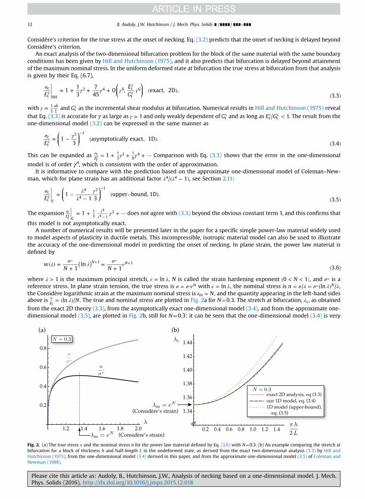
where λ > 1 is the maximum principal stretch, ε λ= ln , N is called the strain hardening exponent ( < < )N0 1 , and σ⁎ is areference stress. In plane strain tension, the true stress is σ σ ε= ⁎ N with ε λ= ln , the nominal stress is σ λ σ λ λ= = ( )⁎n / ln /N ,the Considère logarithmic strain at the maximum nominal stress is ε = Nm , and the quantity appearing in the left-hand sidesabove is λ= ( )σ Nln /
Et. The true and nominal stress are plotted in Fig. 2a for N¼0.3. The stretch at bifurcation, λc, as obtained
from the exact 2D theory (3.3), from the asymptotically exact one-dimensional model (3.4), and from the approximate one-dimensional model (3.5), are plotted in Fig. 2b, still for N¼0.3: it can be seen that the one-dimensional model (3.4) is very
Fig. 2. (a) The true stress s and the nominal stress n for the power law material defined by Eq. (3.6) with N¼0.3. (b) An example comparing the stretch atbifurcation for a block of thickness h and half-length L in the undeformed state, as derived from the exact two-dimensional analysis (3.3) by Hill andHutchinson (1975), from the one-dimensional model (3.4) derived in this paper, and from the approximate one-dimensional model (3.5) of Coleman andNewman (1988).
Please cite this article as: Audoly, B., Hutchinson, J.W., Analysis of necking based on a one-dimensional model. J. Mech.Phys. Solids (2016), http://dx.doi.org/10.1016/j.jmps.2015.12.018i
B. Audoly, J.W. Hutchinson / J. Mech. Phys. Solids ∎ (∎∎∎∎) ∎∎∎–∎∎∎ 13
accurate even for quite stocky blocks. By contrast, the one-dimensional model (3.5) based on an upper bound gives muchless accurate results; consistent with the fact that it overestimates the energy of the bifurcated (necked) solution, this modeldelays the bifurcation artificially, i.e. provides an upper bound for the critical strain. For relatively slender blocks, i.e.
<π 0.5hL2
, all three models predict a critical strain at the onset of necking which is very close to Considère estimate λ ≈ 1.35m .
3.2. Necking behavior of a block of nonlinear elastic material
We proceed to investigate the post-bifurcation behavior of the same block considered above. For prescribed uniformnominal stress n on the ends, the energy of the system is the sum of the 1D energy λ( )W of the block and the potentialenergy Ep,
⎡⎣⎢⎢
⎛⎝⎜
⎞⎠⎟
⎤⎦⎥⎥∫λ λ λ λ λ λ( ) + ( ) = ( ) + ( ) −
( )W E h w
hb
Xn X
2dd
d ,3.7
L
p0
2 2
with λ( )b defined in Eq. (1.2) and n now independent of X. Stationarity of +W Ep with respect to variations of the stretch λ ( )Xgenerates the second order ordinary differential equation and boundary conditions,
⎛⎝⎜
⎞⎠⎟λ λ
λλ λ
λλ− ( ) − ( ) + ( ) =
( )h b
Xh b
Xw
ndd 2
dd
dd
dd 3.8a
22
2
2 2
λ λ( ) = ( ) = ( )X XL
dd
0 0dd
0. 3.8b
This non-linear boundary value problem can be integrated numerically in a straightforward manner using arc-lengthcontinuation (Doedel et al., 2007). Alternatively, it can also be solved by quadrature, thanks to the existence of a firstintegral,
⎛⎝⎜
⎞⎠⎟λ λ λ λ= ( ) − ( ) −
( )C w
hb
Xn
2dd
.3.9
2 2
This first integral is used to construct the solution below. In this respect, our approach has close parallels to the work ofColeman and Newman (1988) that developed and employed a one-dimensional model to study neck development andpropagation relevant to polymer drawing processes. These authors considered nonlinear elastic materials whose nominalstress–strain curves in tension display the up-down-up behavior of some polymers that gives rise to the formation of alocalized neck followed by its spread along the block or bar. The power-law material under consideration here is char-acteristic of metal in that the nominal stress in tension falls monotonically after the maximum load is attained. Conse-quently, once it forms, the neck localizes the deformation and does not spread. Assume the center of the neck is at X¼0 withsymmetry about the center. Denote the stretches at the center and at the right end by λ λ= ( = )X 0L and λ λ= ( = )X LR , withλ λ>L R in the bifurcated solution. The conditions =λ 0
Xdd
at X¼0 and X¼L imply λ λ λ λ= ( ) − = ( ) −C w n w nL L R R. As a result,we have
λ λλ λ
= ( ) − ( )− ( )
nw w
,3.10
L R
L R
and the invariant (3.9) can be rewritten as
λ λ Δ( ) = −( )
bh
X2dd 3.11
where we have defined Δ λ λ λ λ= [( − ) − ( ( ) − ( ))]n w wL L1/2, and we have assumed <λ 0
Xdd
on the interval < <X L0 , in accordwith λ λ>L R. Inserting the expression of n in Eq. (3.10), Δ reads
⎡⎣⎢
⎤⎦⎥Δ λ λ λ λ λ λ λ
λ λλ λλ λ
( ) = − ( ) − ( )−
− ( ) − ( )− ( )
w w w w, , .
3.12L R L
L R
L R
L
L
1/2
Integration of Eq. (3.11) gives the result for λ ( )X ,
∫ λ λΔ λ λ λ
( ′) ′( ′)
=( )λ
λ
( )
b Xh2
d, ,
,3.13X L R
L
with the requirement for meeting the right end condition
∫ λ λΔ λ λ λ
( ′) ′( ′)
=( )λ
λ b Lh2
d, ,
.3.14L RR
L
This solves the problem of finding post-bifurcated solutions: if we regard the stretch at the center of the neck λL as the
Please cite this article as: Audoly, B., Hutchinson, J.W., Analysis of necking based on a one-dimensional model. J. Mech.Phys. Solids (2016), http://dx.doi.org/10.1016/j.jmps.2015.12.018i
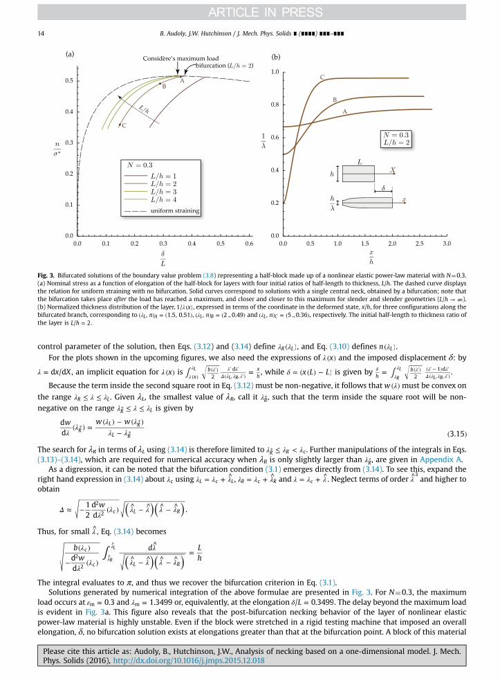
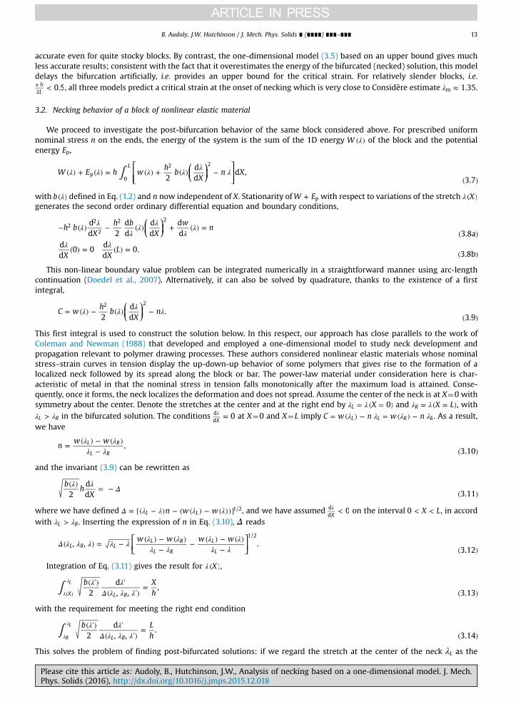
Fig. 3. Bifurcated solutions of the boundary value problem (3.8) representing a half-block made up of a nonlinear elastic power-law material with N¼0.3.(a) Nominal stress as a function of elongation of the half-block for layers with four initial ratios of half-length to thickness, L/h. The dashed curve displaysthe relation for uniform straining with no bifurcation. Solid curves correspond to solutions with a single central neck, obtained by a bifurcation; note thatthe bifurcation takes place after the load has reached a maximum, and closer and closer to this maximum for slender and slender geometries ( → ∞L h/ ).(b) Normalized thickness distribution of the layer, λ ( )x1/ , expressed in terms of the coordinate in the deformed state, x/h, for three configurations along thebifurcated branch, corresponding to λ( ) = ( )n, 1.5, 0.51L A , λ( ) = ( )n, 2 ., 0.49L B and λ( ) = ( )n, 5 ., 0.36L C , respectively. The initial half-length to thickness ratio ofthe layer is =L h/ 2.
B. Audoly, J.W. Hutchinson / J. Mech. Phys. Solids ∎ (∎∎∎∎) ∎∎∎–∎∎∎14
control parameter of the solution, then Eqs. (3.12) and (3.14) define λ λ( )R L , and Eq. (3.10) defines λ( )n L .For the plots shown in the upcoming figures, we also need the expressions of λ ( )x and the imposed displacement δ: by
λ = x Xd /d , an implicit equation for λ ( )x is ∫ =λ
λ λ λ λΔ λ λ λ( )
( ′) ′ ′( ′)x
b xh2
d, ,
L
L R, while δ = ( ( ) − )x L L is given by ∫=δ
λ
λ λ λ λΔ λ λ λ
( ′) ( ′ − ) ′( ′)h
b2
1 d, ,R
L
L R.
Because the term inside the second square root in Eq. (3.12) must be non-negative, it follows that λ( )w must be convex on
the range λ λ λ≤ ≤R L. Given λL, the smallest value of λR, call it λ⁎R, such that the term inside the square root will be non-
negative on the range λ λ λ≤ ≤⁎R L is given by
λλ
λ λλ λ
( ) =( ) − ( )
− ( )⁎
⁎
⁎w w wd
d 3.15RL R
L R
The search for λR in terms of λL using (3.14) is therefore limited to λ λ λ≤ <⁎R R c. Further manipulations of the integrals in Eqs.
(3.13)–(3.14), which are required for numerical accuracy when λR is only slightly larger than λ⁎R, are given in Appendix A.
As a digression, it can be noted that the bifurcation condition (3.1) emerges directly from (3.14). To see this, expand theright hand expression in (3.14) about λc using λ λ λ= + ^
L Lc , λ λ λ= + ^R Rc and λ λ λ= + ^
c . Neglect terms of order λ3and higher to
obtain
( )( )Δλ
λ λ λ λ λ≈ − ( ) ^ − ^ ^ − ^w12
dd
.L R
2
2 c
Thus, for small λ , Eq. (3.14) becomes
( )( )∫λ
λλ
λ
λ λ λ λ
( )
− ( )
^
^ − ^ ^ − ^=
λ
λ
^
^b
wd L
hdd
L R
c2
2 cR
L
The integral evaluates to π, and thus we recover the bifurcation criterion in Eq. (3.1).Solutions generated by numerical integration of the above formulae are presented in Fig. 3. For N¼0.3, the maximum
load occurs at ε = 0.3m and λ = 1.3499m or, equivalently, at the elongation δ =L/ 0.3499. The delay beyond the maximum loadis evident in Fig. 3a. This figure also reveals that the post-bifurcation necking behavior of the layer of nonlinear elasticpower-law material is highly unstable. Even if the block were stretched in a rigid testing machine that imposed an overallelongation, δ, no bifurcation solution exists at elongations greater than that at the bifurcation point. A block of this material
Please cite this article as: Audoly, B., Hutchinson, J.W., Analysis of necking based on a one-dimensional model. J. Mech.Phys. Solids (2016), http://dx.doi.org/10.1016/j.jmps.2015.12.018i

B. Audoly, J.W. Hutchinson / J. Mech. Phys. Solids ∎ (∎∎∎∎) ∎∎∎–∎∎∎ 15
stretched to the bifurcation point would snap dynamically to a state not revealed in Fig. 3a. The curves plotted in Fig. 3a havebeen terminated when the stretch at the center of the neck attains λ ∼ 5L because it is unlikely that the approximations usedin developing the one-dimensional model are valid for deeper necks. If one does carry the model predictions further, onefinds that the extended curves in Fig. 3a intersect the horizontal axis at an elongation much smaller than δc as λ → ∞L . Thus,the model predicts that a block of this material, if stretched to the bifurcation strain, would snap dynamically and “break”when the minimum point of the neck shrinks to zero thickness. For this material, the elastic energy stored in the uniformlystrained layer at the bifurcation point is more than sufficient to drive the layer to neck to a point with the elongation atbifurcation imposed. The limiting behavior in Fig. 3a for a very slender block, → ∞L h/ , would lie on the curve for uniformstraining—except for continuing stretch in the localized neck of width of order h near X¼0, the rest of the block wouldunload by uniform straining.
For a block with initial half-length to thickness ratio, =L h/ 2, the shape of the block at three stages after bifurcation isshown in Fig. 3b as a function of the coordinate in the deformed state x. The width of the neck decreases as localizationproceeds. As a check on the solutions presented in Fig. 3, they have been verified by an independent numerical solution ofthe second order boundary-value problem, based directly on Eq. (3.8), using the library AUTO-07p for numerical con-tinuation (Doedel et al., 2007).
The results of an initial post-bifurcation expansion of the governing differential Eq. (3.8) about the bifurcation point inthe spirit of Koiter (Koiter, 1965; van der Heijden, 2008) can be used to assess the stability at bifurcation and, in particular, toevaluate the initial slope of the load-elongation response at bifurcation seen in Fig. 3a. Denote the uniform stretch infundamental uniform solution by λ0 and the associated nominal stress by λ λ= ( ) = ′( )n n w0 0 0 where λ(·)′ = (·)d /d . The ex-tension of the ends in the fundamental solution is δ λ= −L/ 10 . The bifurcation mode is λ π= ( )X Lcos /1 with λc satisfying (3.1).With ξ as the amplitude of the bifurcation mode, the expansion about λc has the form:
λ λ ξλ ξ λ
λ ξ ξ
λ λ ξ ξ
( ) = + ( ) + ( ) + ⋯
= ′( ) + + ⋯
= + + + ⋯ ( )
X X X
n w n n
a c 3.16
0 12
2
02
24
4
0 c2 4
Regard δ as the prescribed load parameter. Then, ∫ λ =Xd 0L
i0for = …i 1, 2, because the fundamental solution satisfies
δ λ= −L/ 10 . In addition, the mode amplitude is uniquely defined if ∫ λ λ =Xd 0L
i0 1 for >i 1. The important terms for thepresent study are found to be
⎛⎝⎜
⎞⎠⎟
⎛⎝⎜⎜
⎛⎝⎜
⎞⎠⎟
⎞⎠⎟⎟
λ λ π λ
π
π( ) = = −
‴ + ′
″ +( )
XX
L
whL
b
whL
b
cos2
where3
4 43.17a
2 20
20
c
2
c
c
2
c
⎛⎝⎜⎜
⎛⎝⎜
⎞⎠⎟
⎞⎠⎟⎟π= ‴ + ′
( )n w
hL
b14 3.17b
2 c
2
c
⎛⎝⎜⎜
⎛⎝⎜
⎞⎠⎟
⎛⎝⎜⎜
⎞⎠⎟⎟
⎞⎠⎟⎟λ π λ= − ‴ + ⁗ + ′ + ″
( )a
nw w
hL
b b1
324 2 6
3.17c220
c c
2
20
c c
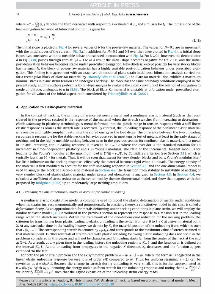
Fig. 4. The initial slope of the post-bifurcation load-elongation behavior for the block of nonlinear power-law material, as obtained by the initial post-bifurcation analysis in Eq. (3.18).
Please cite this article as: Audoly, B., Hutchinson, J.W., Analysis of necking based on a one-dimensional model. J. Mech.Phys. Solids (2016), http://dx.doi.org/10.1016/j.jmps.2015.12.018i
B. Audoly, J.W. Hutchinson / J. Mech. Phys. Solids ∎ (∎∎∎∎) ∎∎∎–∎∎∎16
where λ‴ = ( )λ
w wc
d
d c3
3 denotes the third derivative with respect to λ evaluated at λc, and similarly for ′bc. The initial slope of the
load-elongation behavior of bifurcated solution is given by
δ δ−
( − )= ″ +
( )
n nw
na
.3.18L
c1
cc
2
The initial slope is plotted in Fig. 4 for several values of N for the power-law material. The values for N¼0.3 are in agreementwith the initial slopes of the curves in Fig. 3a. In addition, for N¼0.2 and 0.3 over the range plotted in Fig. 4, the initial slopeis positive, consistent with the unstable behavior discussed in connection with Fig. 3a. For N¼0.1, however, the denominatora in Eq. (3.18) passes through zero at =L h/ 1.6: as a result the initial slope becomes negative for <L h/ 1.6, and the initialpost-bifurcation behavior becomes stable under prescribed elongation. Nevertheless, except possibly for very stocky blockshaving small N, the block of power-law material has a highly unstable post-bifurcation behavior under prescribed elon-gation. This finding is in agreement with an exact two-dimensional plane strain initial post-bifurcation analysis carried outfor a rectangular block of Blatz-Ko material by Triantafyllidis et al. (2007). The Blatz-Ko material also exhibits a maximumnominal stress in plane strain tension and undergoes necking. The block has the same boundary conditions employed in thepresent study, and the authors perform a Koiter-type analysis to evaluate the initial curvature of the relation of elongation tomode amplitude, analogous to a in (3.16). The block of Blatz-Ko material is unstable at bifurcation under prescribed elon-gation for all values of the initial aspect ratio considered by Triantafyllidis et al. (2007).
4. Application to elastic-plastic materials
In the context of necking, the primary difference between a metal and a nonlinear elastic material (such as that con-sidered in the previous section) is the response of the material when the stretch switches from increasing to decreasing—elastic unloading in plasticity terminology. A metal deformed into the plastic range in tension responds with a stiff linearelastic response as soon as the stretch rate is reversed. By contrast, the unloading response of the nonlinear elastic materialis reversible and highly compliant, returning the stored energy as the load drops. The difference between the two unloadingresponses is responsible for the stable necking behavior observed in most tensile test of metals, at least in the early stages ofnecking, and in the highly unstable necking behavior seen in the previous section for nonlinear elastic materials. In a metalin uniaxial stressing, the unloading response is taken to be σ ε = E where the over-dot is the standard notation for anincrement in time-independent plasticity and E is Young's modulus. The ratio of the incremental tangent modulus forloading to the Young's modulus at the maximum load is σ=E E E/ /t
mm , by Considère's criterion (see Section 3.1), which is
typically less than −10 2 for metals. Thus, it will be seen that, except for very slender blocks and bars, Young's modulus itselfhas little influence on the necking response—effectively the material becomes rigid when it unloads. The energy density ofthe material is first modified to account for the stiff unloading response in Section 4.1, and the one-dimensional model isused to analyze the block of elastic-plastic material in Section 4.2. The transition from stability to instability of necking ofvery slender blocks of elastic-plastic material under prescribed elongation is analyzed in Section 4.3. In Section 4.4, wecalculate a coefficient of stress reduction at the center neck by the one-dimensional model, and show that it agrees with thatproposed by Bridgman (1952) up to moderately large necking amplitudes.
4.1. Extending the one-dimensional model to account for elastic unloading
A nonlinear elastic constitutive model is commonly used to model the plastic deformation of metals under conditionswhen the strains increase monotonically and proportionally. In plasticity theory, a constitutive model in this class is called adeformation theory. As an approximation for metals deforming under necking conditions in plane strain, we will employ thenonlinear elastic model (3.6) introduced in the previous section to represent the response to a tension test in the loadingrange when the stretch increases. Within the framework of the one-dimensional reduction for the necking problem, thecriterion for transitioning from plastic loading to elastic unloading is the switch from λ > 0 to λ < 0 at a given material pointX. At any particular time in the loading history, we denote by Xu the material position of the unloading front, which is suchthat λ ( ) =X 0u . The corresponding stretch is denoted by λ ( )Xu u , and corresponds to the maximum value of stretch attained atthat material point. Further reversals of stretch-rate with plastic reloading following elastic unloading does not occur in theproblems considered in this paper and will not be characterized. Unloading starts far from the center of the neck at the endat X¼L. As a result, at any given time in the loading history the unloading region is [ ]X L,u and the function λu is defined onthe interval [ ]X L,u . As the unloading front propagates in the negative X direction, Xu decreases, and the function λu getsextended ‘to the left’.
For both the plane strain problem and the axisymmetric problem, σ λ λ λ = + ≈ n n n , where the term λ n is neglected in thelinear elastic unloading response because it is of order σ E/ compared to λn . Thus, for uniform straining, σ ε = E can berewritten as λ λ = ( ) n E/ 2 . Because the change in stretch during unloading is very small, this is further approximated as
λ λ = ( ) n E/ u2 . With λ( )wu denoting the energy under uniform stretch for the unloading response and noting that λ = λ
λ( )n wd
d
2 u2 ,
we identify λ=λλ
( ) E/wd
d u22 u
2 such that the Taylor expansion of the unloading strain energy reads
Please cite this article as: Audoly, B., Hutchinson, J.W., Analysis of necking based on a one-dimensional model. J. Mech.Phys. Solids (2016), http://dx.doi.org/10.1016/j.jmps.2015.12.018i
B. Audoly, J.W. Hutchinson / J. Mech. Phys. Solids ∎ (∎∎∎∎) ∎∎∎–∎∎∎ 17
λ λ λ λλ
λ λ λ λ( ) = ( ) + ( − ) + ( − ) <( )
w w nE
2for .
4.1u u u u
u2 u
2u
Here, λ λ( ) = ( )w wu u u and = =λλ
λλ
( ) ( )n w wu
dd
dd
u u u as both the strain energy and the nominal stress are continuous at the onset ofunloading.
Observe that the expansion in Eq. (4.1) differs from that of the original strain energy λ( )w (representing the loadingphase) through the quadratic term only. This suggests a modified definition of the strain energy density, which capturesboth loading and unloading:
( )λ αλ
λ λ( ) + −( )
wE
2 4.2au2 u
2
where
⎪
⎧⎨⎩α
λλ λ
= > ( )≤ ( ) ( )
0 for 0 loading
1 for unloading 4.2bu
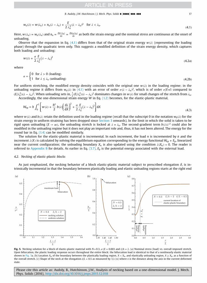
For uniform stretching, the modified energy density coincides with the original one λ( )w in the loading regime; in theunloading regime it differs from λ( )wu in (4.1) with an error of order σ λ λ( − )u
2, which is of order σ ⪡E/ 1 compared toλ λ λ( )( − )E/ u
2u
2. When unloading sets in, λ λ λ( )( − )E/12 u
2u
2 dominates changes in λ( )w for small changes of the stretch from λu.Accordingly, the one-dimensional strain energy W in Eq. (1.2) becomes, for the elastic-plastic material,
⎡⎣⎢⎢
⎛⎝⎜
⎞⎠⎟
⎤⎦⎥⎥∫ ( )λ λ λ α
λλ λ= ( ) + ( ) + −
( )W h w
hb
XE
X2
dd 2
d4.3
L
ep0
2 2
u2 u
2
where λ( )w and λ( )b retain the definition used in the loading regime (recall that the subscript 0 in the notation λ( )w0 for thestrain energy in uniform straining has been dropped since Section 3 onwards). In the limit in which the solid is taken to berigid upon unloading ( → ∞)E , the unloading stretch is locked at λ λ= u. The second-gradient term λ λ( ) ′b 2 could also bemodified in the unloading regime but it does not play an important role and, thus, it has not been altered. The energy for theround bar in Eq. (1.4) can be modified similarly.
The solution for the elastic-plastic material is incremental. In each increment, the load n is incremented by n and theincrement λ ( )X is calculated by solving the equilibrium equation corresponding to the energy functional +W Eep p, linearizednear the current configuration; the unloading boundary Xu is also updated using the condition λ ( ) =X 0u . The reader isreferred to Appendix B for details. As earlier in Eq. (3.7), Ep is the potential energy associated with the external load.
4.2. Necking of elastic-plastic blocks
As just emphasized, the necking behavior of a block elastic-plastic material subject to prescribed elongation δ, is in-trinsically incremental in that the boundary between plastically loading and elastic unloading regions starts at the right end
Fig. 5. Necking solution for a block of elastic-plastic material with N¼0.3, σ =⁎ E/ 0.003 and =L h/ 2. (a) Nominal stress (load) vs. overall imposed stretch.Upon bifurcation, the plastic loading response occurs throughout the entire block: the bifurcation load is identical to that of a nonlinearly elastic materialshown in Fig. 3a. (b) Location Xu of the boundary between the plastically loading region, <X Xu, and elastically unloading region, ≥X Xu, as a function ofthe overall stretch. (c) Shape of the neck at the elongation δ =L/ 0.5 as measured by 1/λ (x) where x is the distance along the axis in the current deformedstate.
Please cite this article as: Audoly, B., Hutchinson, J.W., Analysis of necking based on a one-dimensional model. J. Mech.Phys. Solids (2016), http://dx.doi.org/10.1016/j.jmps.2015.12.018i
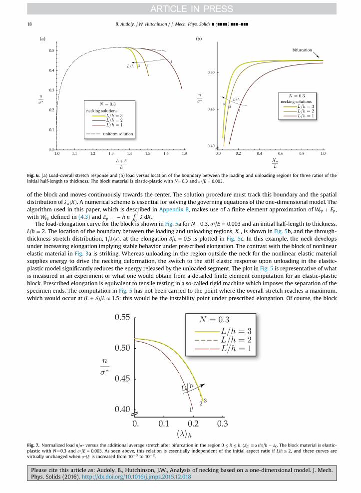
Fig. 6. (a) Load-overall stretch response and (b) load versus location of the boundary between the loading and unloading regions for three ratios of theinitial half-length to thickness. The block material is elastic-plastic with N¼0.3 and σ =⁎ E/ 0.003.
B. Audoly, J.W. Hutchinson / J. Mech. Phys. Solids ∎ (∎∎∎∎) ∎∎∎–∎∎∎18
of the block and moves continuously towards the center. The solution procedure must track this boundary and the spatialdistribution of λ ( )Xu . A numerical scheme is essential for solving the governing equations of the one-dimensional model. Thealgorithm used in this paper, which is described in Appendix B, makes use of a finite element approximation of +W Eep p,with Wep defined in (4.3) and ∫ λ= −E h n Xdp
L
0.
The load-elongation curve for the block is shown in Fig. 5a for N¼0.3, σ =⁎ E/ 0.003 and an initial half-length to thickness,=L h/ 2. The location of the boundary between the loading and unloading regions, Xu, is shown in Fig. 5b, and the through-
thickness stretch distribution, λ ( )x1/ , at the elongation δ =L/ 0.5 is plotted in Fig. 5c. In this example, the neck developsunder increasing elongation implying stable behavior under prescribed elongation. The contrast with the block of nonlinearelastic material in Fig. 3a is striking. Whereas unloading in the region outside the neck for the nonlinear elastic materialsupplies energy to drive the necking deformation, the switch to the stiff elastic response upon unloading in the elastic-plastic model significantly reduces the energy released by the unloaded segment. The plot in Fig. 5 is representative of whatis measured in an experiment or what one would obtain from a detailed finite element computation for an elastic-plasticblock. Prescribed elongation is equivalent to tensile testing in a so-called rigid machine which imposes the separation of thespecimen ends. The computation in Fig. 5 has not been carried to the point where the overall stretch reaches a maximum,which would occur at δ( + ) ≈L L/ 1.5: this would be the instability point under prescribed elongation. Of course, the block
Fig. 7. Normalized load σ⁎n/ versus the additional average stretch after bifurcation in the region ≤ ≤X h0 , λ λ⟨ ⟩ ≡ ( ) −x h h/h c. The block material is elastic-plastic with N¼0.3 and σ =⁎ E/ 0.003. As seen above, this relation is essentially independent of the initial aspect ratio if ≥L h/ 2, and these curves arevirtually unchanged when σ⁎ E/ is increased from 10�3 to 10�2.
Please cite this article as: Audoly, B., Hutchinson, J.W., Analysis of necking based on a one-dimensional model. J. Mech.Phys. Solids (2016), http://dx.doi.org/10.1016/j.jmps.2015.12.018i
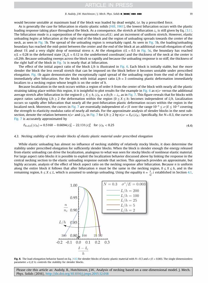
B. Audoly, J.W. Hutchinson / J. Mech. Phys. Solids ∎ (∎∎∎∎) ∎∎∎–∎∎∎ 19
would become unstable at maximum load if the block was loaded by dead weight, i.e. by a prescribed force.As is generally the case for bifurcation in elastic-plastic solids (Hill, 1961), the lowest bifurcation occurs with the plastic
loading response taking place throughout the block. As a consequence, the stretch at bifurcation λc is still given by Eq. (3.1).The bifurcation mode is a superposition of the eigenmode π( )X Lcos / and an increment of uniform stretch. However, elasticunloading begins at bifurcation at the right end of the block and the region of unloading spreads towards the center of theneck, as seen in Fig. 5b. The spread of the unloading region is remarkably rapid. As seen in Fig. 5b, the loading/unloadingboundary has reached the mid-point between the center and the end of the block at an additional overall elongation of onlyabout 1% and a very slight drop of nominal stress n. At the elongation δ =L/ 0.5 in Fig. 5c, the boundary has reached
=x L/ 0.28 in the deformed state ( ≈X L/ 0.12u in the undeformed coordinate) and the thickness of the neck at the center is≈ h0.29 . Because unloading sweeps across the block so rapidly and because the unloading response is so stiff, the thickness ofthe right half of the block in Fig. 5c is nearly that at bifurcation.
The effect of the initial aspect ratio of the block L h/ is illustrated in Fig. 6. Each block is initially stable, but the moreslender the block the less overall stretch that can be imposed on the block before it becomes unstable under prescribedelongation. Fig. 6b again demonstrates the exceptionally rapid spread of the unloading region from the end of the blockimmediately after bifurcation. For the block with initial aspect ratio =L h/ 3 continuing plastic deformation immediatelylocalizes to a necking region whose length is on the order of h.
Because localization in the neck occurs within a region of order h from the center of the block with nearly all the plasticstraining taking place within this region, it is insightful to plot results for the example in Fig. 6 as σ⁎n/ versus the additionalaverage stretch after bifurcation in the region ≤ ≤X h0 , λ λ⟨ ⟩ ≡ ( ) −x h h/h c, as in Fig. 7. This figure reveals that for blocks withaspect ratios satisfying ≥L h/ 2 the deformation within the region ( ≤ ≤ )X h0 becomes independent of L h/ . Localizationoccurs so rapidly after bifurcation that nearly all the post-bifurcation plastic deformation occurs within the region in thelocalized neck. Moreover, the curves in Fig. 7 are essentially independent of σ⁎ E/ over the range σ≤ ≤− ⁎ −E10 / 103 2 coveringthe strength to elasticity modulus ratio of nearly all metals. For the approximate analysis of slender blocks in the next sub-section, denote the relation between σ⁎n/ and λ⟨ ⟩h in Fig. 7 for ≥L h/ 2 by σ λ= (⟨ ⟩ )⁎n F/ N h . Specifically, for N¼0.3, the curve inFig. 7 is accurately approximated by
( )λ λ λ λ⟨ ⟩ = − ⟨ ⟩ − ⟨ ⟩ ⟨ ⟩ < ( )=F 0.5160 0.6694 22.131 for 0.25 4.4N h h h h0.32 4
4.3. Necking stability of very slender blocks of elastic-plastic material under prescribed elongation
While elastic unloading has almost no influence of necking stability of relatively stocky blocks, it does determine thestability under prescribed elongation for sufficiently slender blocks. When the block is slender enough the energy releasedfrom elastic unloading can drive the localization, analogous to what was seen for stocky blocks of nonlinear elastic material.For large aspect ratio blocks it is possible to exploit the localization behavior discussed above by linking the response in thecentral necking section to the elastic unloading response outside that section. This approach provides an approximate, buthighly accurate, analysis of the effect of block aspect ratio on the necking response after bifurcation. Because n is uniformalong the entire block it follows that after bifurcation n must be the same in the necking region, ≤ ≤X h0 , and in theremaining region, ≤ ≤h X L, which is assumed to undergo unloading. Using the equality λ =
λn n
u2 established in Section 4.1,
Fig. 8. The load-elongation behavior based on Eq. (4.6) for slender blocks of elastic-plastic material with N¼0.3 and σ =⁎ E/ 0.003. The single dimensionlessparameter σ ( )⁎L E h/ controls the stability for slender blocks.
Please cite this article as: Audoly, B., Hutchinson, J.W., Analysis of necking based on a one-dimensional model. J. Mech.Phys. Solids (2016), http://dx.doi.org/10.1016/j.jmps.2015.12.018i
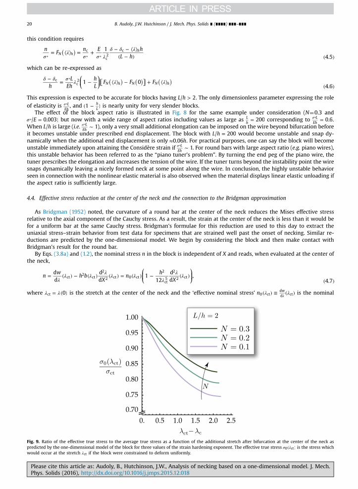
B. Audoly, J.W. Hutchinson / J. Mech. Phys. Solids ∎ (∎∎∎∎) ∎∎∎–∎∎∎20
this condition requires
( )σ
λσ σ λ
δ δ λ= ⟨ ⟩ = + − − ⟨ ⟩( − ) ( )⁎ ⁎ ⁎
nF
n E hL h
14.5
N hhc
c2
c
which can be re-expressed as
⎛⎝⎜
⎞⎠⎟⎡⎣ ⎤⎦( ) ( ) ( )δ δ σ λ λ λ− = − ⟨ ⟩ − + ⟨ ⟩
( )
⁎
hL
EhhL
F F F1 04.6
N h N N hc
c2
This expression is expected to be accurate for blocks having >L h/ 2. The only dimensionless parameter expressing the role
of elasticity is σ⁎LEh, and ( − )1 h
Lis nearly unity for very slender blocks.
The effect of the block aspect ratio is illustrated in Fig. 8 for the same example under consideration (N¼0.3 andσ = )⁎ E/ 0.003 but now with a wide range of aspect ratios including values as large as = 200L
hcorresponding to =σ⁎
0.6LEh
.When L h/ is large (i.e. ∼σ⁎
1LEh
), only a very small additional elongation can be imposed on the wire beyond bifurcation beforeit becomes unstable under prescribed end displacement. The block with =L h/ 200 would become unstable and snap dy-namically when the additional end displacement is only ≈ h0.06 . For practical purposes, one can say the block will becomeunstable immediately upon attaining the Considère strain if ∼σ⁎
1LEh
. For round bars with large aspect ratio (e.g. piano wires),this unstable behavior has been referred to as the “piano tuner's problem”. By turning the end peg of the piano wire, thetuner prescribes the elongation and increases the tension of the wire. If the tuner turns beyond the instability point the wiresnaps dynamically leaving a nicely formed neck at some point along the wire. In conclusion, the highly unstable behaviorseen in connection with the nonlinear elastic material is also observed when the material displays linear elastic unloading ifthe aspect ratio is sufficiently large.
4.4. Effective stress reduction at the center of the neck and the connection to the Bridgman approximation
As Bridgman (1952) noted, the curvature of a round bar at the center of the neck reduces the Mises effective stressrelative to the axial component of the Cauchy stress. As a result, the strain at the center of the neck is less than it would befor a uniform bar at the same Cauchy stress. Bridgman's formulae for this reduction are used to this day to extract theuniaxial stress–strain behavior from test data for specimens that are strained well past the onset of necking. Similar re-ductions are predicted by the one-dimensional model. We begin by considering the block and then make contact withBridgman's result for the round bar.
By Eqs. (3.8a) and (1.2), the nominal stress n in the block is independent of X and reads, when evaluated at the center ofthe neck,
⎛⎝⎜
⎞⎠⎟λ
λ λ λ λ λλ
λ λ= ( ) − ( ) ( ) = ( ) − ( )( )
nw
h bX
nh
Xdd
dd
112
dd
,4.7
ct2
ct
2
2 ct 0 ct
2
ct5
2
2 ct
where λ λ= ( )0ct is the stretch at the center of the neck and the ‘effective nominal stress’ λ λ( ) ≡ ( )λ
n w0 ct
dd ct is the nominal
Fig. 9. Ratio of the effective true stress to the average true stress as a function of the additional stretch after bifurcation at the center of the neck aspredicted by the one-dimensional model of the block for three values of the strain hardening exponent. The effective true stress σ λ( )0 ct is the stress whichwould occur at the stretch λct if the block were constrained to deform uniformly.
Please cite this article as: Audoly, B., Hutchinson, J.W., Analysis of necking based on a one-dimensional model. J. Mech.Phys. Solids (2016), http://dx.doi.org/10.1016/j.jmps.2015.12.018i
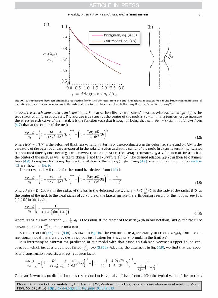
Fig. 10. (a) Comparison between Bridgman's ‘correction factor’ and the result from the one-dimensional reduction for a round bar, expressed in terms ofthe ratio ρ of the cross-sectional radius to the radius of curvature at the center of neck. (b) Using Bridgman's notation, ρ = a R/B B.
B. Audoly, J.W. Hutchinson / J. Mech. Phys. Solids ∎ (∎∎∎∎) ∎∎∎–∎∎∎ 21
stress if the stretch were uniform and equal to λct. Similarly, the ‘effective true stress’ is σ λ( )0 ct , where σ λ λ λ( ) = ( )nct ct0 ct 0 is thetrue stress at uniform stretch λct. The average true stress at the center of the neck is σ λ= nct ct . In a tension test to measurethe stress-stretch curve of the metal, it is the function σ λ( )0 that is sought. Noting that σ λ σ λ( ) = ( )n n/ /0 ct ct 0 ct , it follows from(4.7) that at the center of the neck
⎛⎝⎜
⎞⎠⎟
⎛⎝⎜
⎞⎠⎟
σ λσ λ
λ λ( ) = − ( ) = + ( ) ( )( )
− −h
Xh h
x1
12dd
10
12dd
04.8
0 ct
ct
2
ct5
2
2 ct
1 2
2
1
where λ( ) = ( )h x h x/ is the deformed thickness variation in terms of the coordinate x in the deformed state and h xd /d2 2 is thecurvature of the outer boundary measured in the axial direction and at the center of the neck. In a tensile test, σ λ( )0 ct cannotbe measured directly once necking starts. However, one can measure the average true stress σct as a function of the stretch atthe center of the neck, as well as the thickness h and the curvature h xd /d2 2. The desired relation σ λ( )0 can then be obtainedfrom (4.8). Examples illustrating the direct calculation of the ratio σ λ σ( )/0 ct ct using (4.8) based on the simulations in Section4.2 are shown in Fig. 9.
The corresponding formula for the round bar derived from (1.4) is
⎛⎝⎜
⎞⎠⎟
⎛⎝⎜
⎞⎠⎟
σ λσ λ
λ λ( ) = − ( ) = + ( ) ( ) =+ ( )
ρ
− −DX
R Rx
132
dd
10
4dd
01
1,
4.90 ct
ct
2
ct4
2
2 ct
1 2
2
1
4
where λ( ) = ( ( ) )R x D x/ 2 is the radius of the bar in the deformed state, and ρ = ( ) ( )R 0 0R
x
d
d
2
2 is the ratio of the radius ( )R 0 at
the center of the neck to the axial radius of curvature of the lateral surface there. Bridgman's result for this ratio is (see Eqs.(1)–(13) in his book)
( ) ( )σ λ
σ( ) =
+ + ( )ρρ
1
1 ln 1,
4.10
0 ct
ct B2
2
where, using his own notation, ρ = aR
B
B, aB is the radius at the center of the neck ( ( )R 0 in our notation) and RB the radius of
curvature there ( ( )1/ 0R
x
d
d
2
2 in our notation).
A comparison of (4.9) and (4.10) is shown in Fig. 10. The two formulae agree exactly to order ρ = a R/B B. Our one-di-mensional model therefore provides a rigorous justification for Bridgman's formula in the limit ρ⪡1.
It is interesting to contrast the prediction of our model with that based on Coleman-Newman's upper bound con-
struction, which includes a spurious factor λλ − 1
3
3, see (2.32b). Adapting the argument in Eq. (4.9), we find that the upper
bound construction predicts a stress reduction factor
⎜ ⎟
⎛⎝⎜
⎞⎠⎟
⎛⎝⎜
⎞⎠⎟ ⎛
⎝⎞⎠
σ λσ λ
λλ
λ λ λλ
( ) = −−
( ) = +−
( ) ( ) =+λ
λ
ρ
− −
−
DX
R Rx
132 1
dd
11
04
dd
01
1.0 ct
ct C
2
ct4
ct3
ct3
2
2 ct
1ct3
ct3
2
2
1
1 4ct3
ct3
Coleman–Newman's prediction for the stress reduction is typically off by a factor ∼40% (the typical value of the spurious
Please cite this article as: Audoly, B., Hutchinson, J.W., Analysis of necking based on a one-dimensional model. J. Mech.Phys. Solids (2016), http://dx.doi.org/10.1016/j.jmps.2015.12.018i
B. Audoly, J.W. Hutchinson / J. Mech. Phys. Solids ∎ (∎∎∎∎) ∎∎∎–∎∎∎22
factor in the denominator is 1.81, as noted earlier). In addition, the spurious factor brings in an additional dependence on thestretch λct and the stress reduction is not a function of ρ only—in contrast with Bridgman's formula (4.9) and ours (4.10).
This shows that Bridgman's formula captures a subtle feature of necking, revealed by the asymptotically exact 1D-model:the existence of a simple relation between the stress reduction factor σ λ σ( )/0 ct ct and the geometric parameter ρ. The lessaccurate upper-bound construction of Coleman–Newman fails to capture this feature.
5. Conclusions and suggestions for further research
A one-dimensional model has been derived for the necking analysis of rectangular blocks and round bars. It is carried outwithin the framework of nonlinear elastic solids but it has been extended for applications to elastic-plastic solids. By in-corporating gradients of the strains that arise during necking, the model is capable of capturing the highly nonlinear lo-calization process that accompanies necking. Bifurcation from the uniform state into the necking mode is accurately re-produced by the model. Moreover, comparison with the widely employed Bridgman formula for extracting uniaxial stress–strain behavior from data measured from a necked specimen suggests that the one-dimensional model remains accurate forrelatively deep necks.
The dimensional reduction carried out in this paper takes into account the curvature of the material lines initially normalto the axis of the slab or bar. This turned out to be crucial for the correctness of the dimensional reduction, as it is otherwiseimpossible to relax the shear stress at the free boundaries. This curvature effect has been ignored in prior work on ax-isymmetric bars where material lines have been assumed to remain normal to the axis, resulting in a second-gradient modelwhich is formally similar to the asymptotically exact one but overestimates the modulus of the second-gradient term. Infuture work, it would be interesting to extend the present work and take into account this curvature effect in the derivationof second-gradient models coupled to physical fields, such as thin elastic biomembranes coupled to the concentration ofchemical species (Deseri et al., 2008), or elastic membranes to an electric field (De Tommasi et al., 2013).
In this paper the model has been used to demonstrate the exceptional difference between the necking behavior ofnonlinear elastic materials and elastic-plastic materials. For nonlinear elastic materials which have a maximum load underuniform tension, bifurcation into a necking mode occurs shortly beyond attainment of the maximum load and is highlyunstable, snapping dynamically under prescribed elongation. By contrast, the post-bifurcation response of an elastic-plasticmaterial specimen displays stable behavior for a range of elongations beyond the maximum load. The extent of the stablerange depends on the slenderness of the specimen. Very slender specimens such as long wires or thin sheets lose stabilityalmost immediately upon attaining the maximum load with all plastic deformation localized at a neck which shrinks to zerocross-section.
The one-dimensional model facilitates analytical investigations of necking and localization. Coleman and Newman(1988) developed an earlier version of the model for the purpose of studying the drawing process of polymer fibers' steady-state neck propagation in materials which undergo a local maximum load under uniaxial tension followed by strengtheningwith further stretching. The model holds promise for advancing the understanding of other important necking phenomena.If it can be extended to encompass rate-dependent material behavior, it will provide a valuable extension of the long-wavelength approximation used by Hutchinson and Neale (1977) and Ghosh (1977) to analyze the significant influence ofmaterial strain-rate sensitivity on necking in the tensile test. Rate-sensitivity becomes increasingly important at highertemperatures and its influence on necking is not well characterized. The one-dimensional model should be well suited forinvestigating phenomena such as the occurrence of multiple necks.
Another area of potential application for the one-dimensional model is sheet metal necking. The Marciniak–Kuczyńskimodel (Marciniak and Kuczyński, 1967) is a long-wavelength approximation for predicting the onset of necking in sheetssubject to general combinations of in-plane stretch. The outcome of such analyses is the forming limit diagram used todesign metal forming processes. By including the influence of the gradients of the strain, the one-dimensional model wouldpredict detailed spatial aspects of neck development in the sheet which the long-wavelength approximation does notprovide. In the range of imposed in-plane strains in which the localized neck is not perpendicular to the maximum principlestrain, the one-dimensional model would have to be extended to include shearing strains parallel to the localization band.For sheet metal necking and other necking problems, it is straightforward to account for initial imperfections in the model.
Appendix A. Manipulation of integrals
Numerical integration of the integrals in Eqs. (3.13)–(3.14) is required to generate the curves in Section 3. These integralsare ill-conditioned at their lower limit when λ λ≅ ⁎
R R defined in (3.15), which occurs for all but stocky blocks. In the following,the integrals are manipulated into a form that extracts the analytical dependence on λR as λ λ→ *R R resulting in integralswhich are well-condition for numerical integration. Consider (3.14):
∫ λλ′
( ′)=
( )λ
λ dR
Lh A.1R
L
Please cite this article as: Audoly, B., Hutchinson, J.W., Analysis of necking based on a one-dimensional model. J. Mech.Phys. Solids (2016), http://dx.doi.org/10.1016/j.jmps.2015.12.018i
B. Audoly, J.W. Hutchinson / J. Mech. Phys. Solids ∎ (∎∎∎∎) ∎∎∎–∎∎∎ 23
where
( )λ Δ λ λ λλ λ
λ λ λ λ( ) = ( )( )
=( )
( ) − ˜ ( )Rb b
w w2 , , 2
, ,L RR L
2
and
λ λ λ λ λ λ λ λ λλ λ
˜ ( ) = ( )( − ) + ( )( − )−
ww w
, , .R LR L L R
L R
The Taylor expansion of λ( )R at λ λ= R reads λ λ λ λ λ( ) = ( − ) + ( − ) + ⋯R A BR R2 , where
⎡⎣⎢
⎤⎦⎥
⎡⎣⎢
⎤⎦⎥
λλ
λ λ λλ λ
λ λλ
λ λ λλ λ λ
λ
= ′( ) =( )
′( ) − ( ) − ( )−
= ″( ) = −′( )
( )′( ) − ( ) − ( )
−+
( )″( )
A Rb
ww w
B Rb
bw
w wb
w
2
12
2 1
RR
RL R
L R
RR
RR
L R
L R RR2
and λ(·)′ = (·)d /d . At λ λ= L, the Taylor expansion reads λ λ λ( ) = ( − ) + ⋯R C L , where
⎡⎣⎢
⎤⎦⎥λ
λλ λλ λ
λ= ′( ) =( )
( ) − ( )−
− ′( )C Rb
w ww
2L
L
L R
L RL
For the functions λ( )w of interest, ≥A 0, >B 0 and >C 0, but →A 0 as λ λ→ ⁎R R by definition of λ⁎
R. As a result, theintegrand in (A.1) is not integrable at the lower limit as λ λ→ ⁎
R R, although it is integrable at λL. Divide the integral into twocontributions: λ λ λ≤ ≤R M and λ λ λ≤ ≤M L with λ λ λ= ( + )/2M R L . Let λ λ λ λ λ( ) = ( − ) + ( − )f A BR R
2 and rewrite (A.1) as
⎛⎝⎜⎜
⎞⎠⎟⎟∫ ∫ ∫ ∫λ
λ λ λλ λ
λλλ
′( ′)
=( ′)
−( ′)
′ +′
( ′)+
′( ′) ( )λ
λ
λ
λ
λ
λ
λ
λ
R R f f Rd 1 1
dd d
.A.2R
L
R
M
R
M
M
L
The first and third integrals above are bounded as λ λ→ ⁎R R and can be integrated numerically with due regard for the end-
point singularity. The second integral is given by
⎛⎝⎜
⎞⎠⎟∫ λ
λλ λ′
( ′)= ( − )
( )λ
λ−
f BB
Ad 2
sinhA.3
M R1
R
M
Manipulation of the other integrals such as (3.13) and those appearing below Eq. (3.14) is also required and similar.
Appendix B. Numerical method for solving the necking problem with linear elastic unloading
The energy functional governing the block is +W Eep p, with Wep given by (4.3). We start by deriving the equation ofequilibrium in weak form by canceling the first variation of +W Eep p for any virtual increment λ of the stretch,
⎡⎣⎢
⎤⎦⎥∫ λ λ λ λ λ α
λλ λ λ λ= ′^ + ′ ′ ^ + ′^′ + ( − ) ^ − ^h w
hb h b
En X0
2d .
L
0
22 2
u2 u
Integrating by parts, one could find an equation which extends the o.d.e. (3.8) and accounts for unloading, but it is pre-ferable to continue working with the weak form.
The simulation solves for increments λ ( )X of the stretch, in terms of increments n of the load, with λ ( )X known from theprevious step. The incremental equation of equilibrium is obtained by linearizing the above weak form (second variation ofthe energy),
⎡⎣⎢⎢
⎛⎝⎜⎜
⎞⎠⎟⎟
⎤⎦⎥⎥∫ λ α
λλλ λ λλ λ λ λ= ″ + ″ ′ + ^ + ′ ′ ( ^) + ′ ^′ − ^h w
hb
Eh b
Xh b n X0
2d
dd .
L
0
22
u2
2 2
Integrating by parts and dropping the boundary term, we have
⎡⎣⎢
⎛⎝⎜
⎞⎠⎟
⎤⎦⎥∫ λ λ α
λλλ λ λ λ= ″ + ″ ′ − ( ′ ′) + ^ + ′^′ − ^h w
hb h
bX
Eh b n X0
2d
dd ,
L
0
22 2
u2
2
which can be simplified as
⎡⎣⎢
⎛⎝⎜
⎞⎠⎟
⎤⎦⎥∫ λ λ α
λλλ λ λ λ= ″ − ″ ′ − ′ ″ + ^ + ′^′ − ^h w
hb h b
Eh b n X0
2d .
L
0
22 2
u2
2
Renaming the increment λ as λ , this equation can be seen as the condition of stationarity of a potential
Please cite this article as: Audoly, B., Hutchinson, J.W., Analysis of necking based on a one-dimensional model. J. Mech.Phys. Solids (2016), http://dx.doi.org/10.1016/j.jmps.2015.12.018i
B. Audoly, J.W. Hutchinson / J. Mech. Phys. Solids ∎ (∎∎∎∎) ∎∎∎–∎∎∎24
⎡⎣⎢
⎛⎝⎜
⎞⎠⎟
⎤⎦⎥∫λ λ λ α
λλ λ λ( ) = ″ − ″ ′ − ′ ″ +
+ ( ′) −
( )F w
hb h b
Eh b n X
2 2 2d .
B.1
L
0
22 2
u2
22
2
In the simulation, suppose λ ( )X is known in the current state and the current location of the boundary between theloading and unloading regions is =X Xu with λ ( )Xu known for ≥X Xu from previous iterations (the stretch λ ( )Xu at whichunloading starts at a given point X is an essential unknown of the simulation). In Eq. (B.1), we then take α = 1 for ≥X Xu andα = 0 for <X Xu. The next increment of stretch λ ( )X is found by rendering the quadratic functional λ( )F stationary, subject toprescribed negative increments of n: this is equivalent to solving the linearized equilibrium. The rapid spread of the un-loading region requires special attention as will be discussed shortly.
To generate numerical results a simple finite element-like scheme is adopted. The interval ≤ ≤X L0 is divided into Mequal length segments and a piecewise linear approximation to λ ( )X is sought in terms of its nodal values λi at the ends ofthe segments Xi, =i M0, . At the current stage of deformation, the contributions to the coefficients in (B.1) depend on λ ( )X ,λ′( )X and λ″( )X . These are evaluated at the interval mid-points using standard finite difference expressions, as are theexpressions for the increments λ and λ′. Summing the mid-point contributions to (B.1) gives the algebraic approximation
∑ ∑λ λ λ= − ( )= =
F C n c .B.2i j
M
ij i ji
M
i i, 0 0
The boundary conditions at the ends are natural, meaning that no constraint on λ0 or λM is required in rendering F stationary.In principle, one could use n as the prescribed control parameter in a step-by-step incremental solution procedure, but
given the exceptionally strong dependence of Xu on n seen in Fig. 6b, it is preferable to prescribe increments of the un-loading boundary Xu and compute the associated increment n. This procedure has been adopted here. Specifically, thecomputation was devised to shift the unloading boundary by exactly one interval, say from +Xk 1 to Xk, and n is chosen tosatisfy the condition λ = 0k at the end of the step. With square brackets denoting matrices and vectors, the stationaritycondition for F in (B.2) is λ[ ] = [ ] ·[ ] −C cn
21 . If [ ]C and [ ]c are evaluated at the start of the incremental step (and are therefore
independent of λ[ ]), λk is proportional to n by the stationarity condition for F, implying that λ = 0k cannot select the value ofn. This dictates that [ ]C and [ ]c should be evaluated using stretch values at the end of the step, λ λ[ + ]: an iterative procedureis required to obtain n for each incremental advance of the unloading boundary. When n and λ[ ] are obtained such thatλ = 0k , the stretch values are updated for the next unloading step and λ ( )Xku is assigned. The numerical results plotted inSection 4 have been computed with M¼200. Curves computed with M¼100 are virtually indistinguishable from thosepresented in Section 4.
References
Antman, S.S., 1973. Nonuniqueness of equilibrium states for bars in tension. J. Math. Anal. Appl. 44 (2), 333–349.Antman, S.S., Carbone, E.R., 1977. Shear and necking instabilities in nonlinear elasticity. J. Elast. 7 (2), 125–151.Bridgman, P.W., 1952. Studies in Large Plastic Flow and Fracture, Metallurgy and Metallurgical Engineering Series. Mc-Graw-Hill, New York.Chen, W.H., 1971. Necking of a bar. Int. J. Solids Struct. 7 (7), 685–717.Coleman, B.D., Newman, D.C., 1988. On the rheology of cold drawing. I. Elastic materials. J. Polym. Sci.: Part B: Polym. Phys. 26, 1801–1822.Considère, A., 1885. Mémoire sur l'emploi du fer et de l'acier dans les constructions. Ann. Ponts Chaussées, Série 6 (9), 574–775.De Tommasi, D., Puglisi, G., Zurlo, G., 2013. Electromechanical instability and oscillating deformations in electroactive polymer films. Appl. Phys. Lett. 102,
011903.Deseri, L., Piccioni, M.D., Zurlo, G., 2008. Derivation of a new free energy for biological membranes. Contin. Mech. Thermodyn. 20 (5), 255–273.Doedel, E.J., Champneys, A.R., Fairgrieve, T.F., Kuznetsov, Y.A., Sandstede, B., Wang, X.J., 2007. AUTO-07p: continuation and bifurcation software for ordinary
differential equations. See ⟨http://indy.cs.concordia.ca/auto/⟩.Ericksen, J.L., 1975. Equilibrium of bars. J. Elast. 5 (3–4), 191–201.Ghosh, A.K., 1977. Tensile instability and necking in materials with strain hardening and strain-rate hardening. Acta Metall. 12 (25), 1413–1424.Hill, R., 1961. Bifurcation and uniqueness in nonlinear mechanics of continua. In: Problems in continuum Mechanics (Muskhelishvili Anniversary Volume),
SIAM, Philadelphia (PA), pp. 155–164.Hill, R., Hutchinson, J.W., 1975. Bifurcation phenomena in the plane tension test. J. Mech. Phys. Solids 23 (4–5), 239–264.Hutchinson, J.W., Miles, J.P., 1974. Bifurcation analysis of the onset of necking in an elastic/plastic cylinder under uniaxial tension. J. Mech. Phys. Solids 22,
61–71.Hutchinson, J.W., Neale, K.W., 1977. Influence of strain-rate sensitivity on necking under uniaxial tension. Acta Metall. 25, 839–846.Koiter, W.T., 1965. On the stability of elastic equilibrium (Ph.D. thesis), Delft University, Holland.Marciniak, K., Kuczyński, K., 1967. Limit strains in the process of stretch forming sheet metal. Int. J. Mech. Sci. 9, 609–620.Mielke, A., 1991. Hamiltonian and Lagrangian flows on center manifolds, with application to elliptic variational problems. Lecture Notes in Mathematics.
vol. 1489. Springer-Verlag, Berlin.Needleman, A., 1972. A numerical study of necking in circular cylindrical bar. J. Mech. Phys. Solids 20 (2), 111–127.Norris, D.M., Moran, B., Scudder, J.K., Quiñones, D.F., 1978. A computer simulation of the tension test. J. Mech. Phys. Solids 26 (1), 1–19.Owen, N., 1987. Existence and stability of necking deformations for nonlinearly elastic rods. Arch. Rational Mech. Anal. 98 (4), 357–383.Scherzinger, W., Triantafyllidis, N., 1998. Asymptotic analysis of stability for prismatic solids under axial loads. J. Mech. Phys. Solids 46 (6), 955–1007.Sivaloganathan, J., Spector, S.J., 2011. On the stability of incompressible elastic cylinders in uniaxial extension. J. Elast. 105 (1–2), 313–330.Triantafyllidis, N., Scherzinger, W.M., Huang, H.-J., 2007. Post-bifurcation equilibria in the plane-strain test of a hyperelastic rectangular block. Int. J. Solids
Struct. 44 (11–12), 3700–3719.van der Heijden, A.M.A., 2008. W.T. Koiter's Elastic Stability of Solids and Structures. Cambridge University Press, Cambridge University, Cambridge, UK.
Please cite this article as: Audoly, B., Hutchinson, J.W., Analysis of necking based on a one-dimensional model. J. Mech.Phys. Solids (2016), http://dx.doi.org/10.1016/j.jmps.2015.12.018i


![Research Article 3-Dimensional Microorifice Fabricated ... · emulsi cation techniques including T-junction shearing [ ], ow focus necking [ , ], and pneumatic pumping [ ] have been](https://img.pdfslide.us/doc/110x75/60a1d19f6750e5772e44a4cb/research-article-3-dimensional-microorifice-fabricated-emulsi-cation-techniques.jpg)