Embed Size (px)
Citation preview

Analysis of Multivariate� Ecological Data
School on Recent Advances in Analysis of Multivariate Ecological Data24-28 October 2016
Prof. Pierre LegendreDr. Daniel Borcard
Département de sciences biologiquesUniversité de Montréal
C.P. 6128, succursale Centre VilleMontréal QC
H3C 3J7 [email protected]@umontreal.ca

2
Day 3

3
Day 3
Statistical testing by permutations

4
Statistical testing by permutations
! see course material by Pierre Legendre
5
Statistical tests for multivariate data
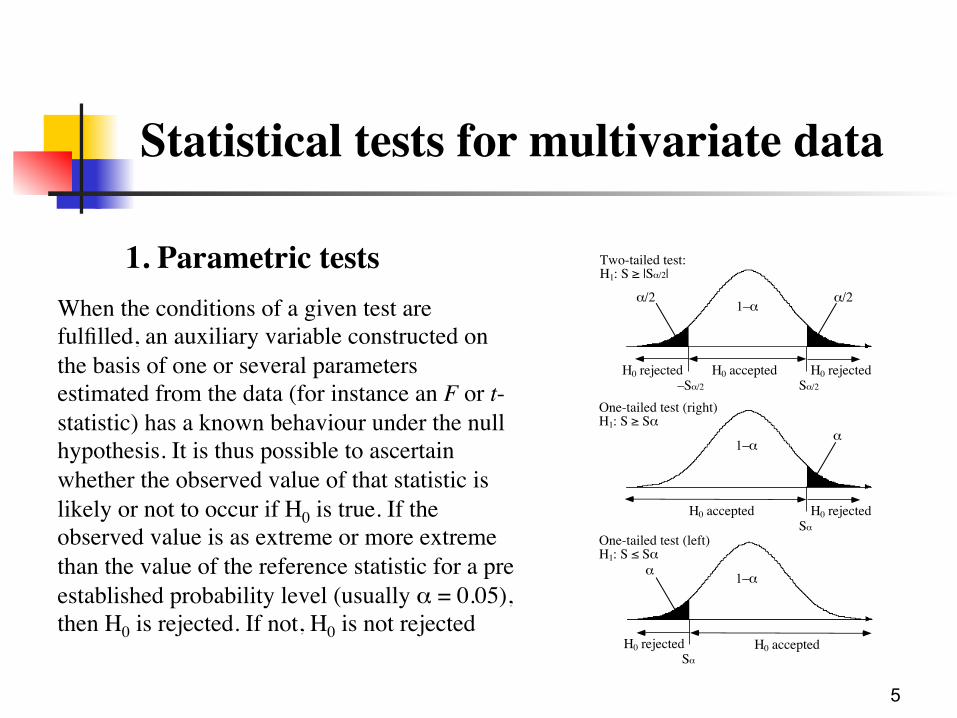
1. Parametric testsWhen the conditions of a given test are fulfilled, an auxiliary variable constructed on the basis of one or several parameters estimated from the data (for instance an F or t-statistic) has a known behaviour under the null hypothesis. It is thus possible to ascertain whether the observed value of that statistic is likely or not to occur if H0 is true. If the observed value is as extreme or more extreme than the value of the reference statistic for a pre established probability level (usually α = 0.05), then H0 is rejected. If not, H0 is not rejected
1–αα
SαH0 acceptedH0 rejected
One-tailed test (left)H1: S ≤ Sα
1–αα
SαH0 accepted H0 rejected
One-tailed test (right)H1: S ≥ Sα
1–αα/2 α/2
H0 accepted H0 rejectedH0 rejected–Sα/2 Sα/2
Two-tailed test:H1: S ≥ |Sα/2|
6
Statistical tests for multivariate data
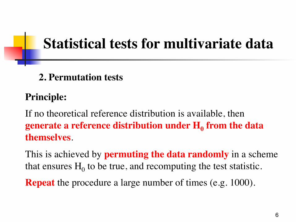
2. Permutation tests
Principle:If no theoretical reference distribution is available, then generate a reference distribution under H0 from the data themselves.
This is achieved by permuting the data randomly in a scheme that ensures H0 to be true, and recomputing the test statistic. Repeat the procedure a large number of times (e.g. 1000).
7
Statistical tests for multivariate data
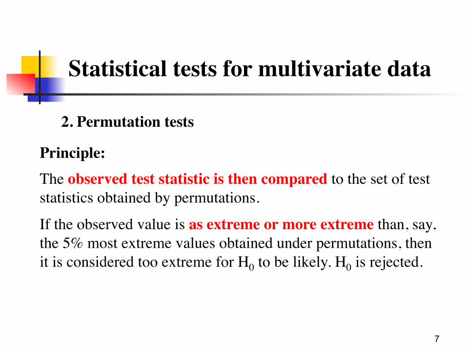
2. Permutation tests
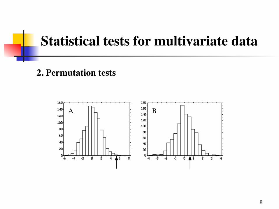
Principle:The observed test statistic is then compared to the set of test statistics obtained by permutations.
If the observed value is as extreme or more extreme than, say, the 5% most extreme values obtained under permutations, then it is considered too extreme for H0 to be likely. H0 is rejected.
8
Statistical tests for multivariate data
2. Permutation tests
A B
9
Statistical tests for multivariate data
2. Permutation testsWords of caution (permutation tests)The method of permutations does not solve all the problems related to statistical testing.
1. Some problems may require different and more complicated permutation schemes than the simple random scheme applied here. Example: tests of the main factors of an ANOVA, where the permutations for factor A must be limited within the levels of factor B, and vice versa.
10
Statistical tests for multivariate data
2. Permutation testsWords of caution (permutation tests)2. Permutation tests do solve several distributional problems, but not all. In particular, they do not solve distributional problems linked to the hypothesis being tested.
For instance, permutational ANOVA does not require normality, but it still does require homogeneity of variances: actually two hypotheses are tested simultaneously, i.e. equality of the means and equality of the variances.
11
Statistical tests for multivariate data
2. Permutation testsWords of caution (permutation tests)3. Contrary to popular belief, permutation tests do not solve the problem of independence of observations. This problem has still to be addressed by special solutions, differing from case to case, and often related to the correction of degrees of freedom.
12
Statistical tests for multivariate data
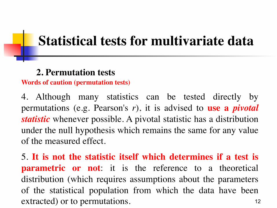
2. Permutation testsWords of caution (permutation tests)
4. Although many statistics can be tested directly by permutations (e.g. Pearson's r), it is advised to use a pivotal statistic whenever possible. A pivotal statistic has a distribution under the null hypothesis which remains the same for any value of the measured effect.
5. It is not the statistic itself which determines if a test is parametric or not: it is the reference to a theoretical distribution (which requires assumptions about the parameters of the statistical population from which the data have been extracted) or to permutations.
13
Statistical tests for multivariate data
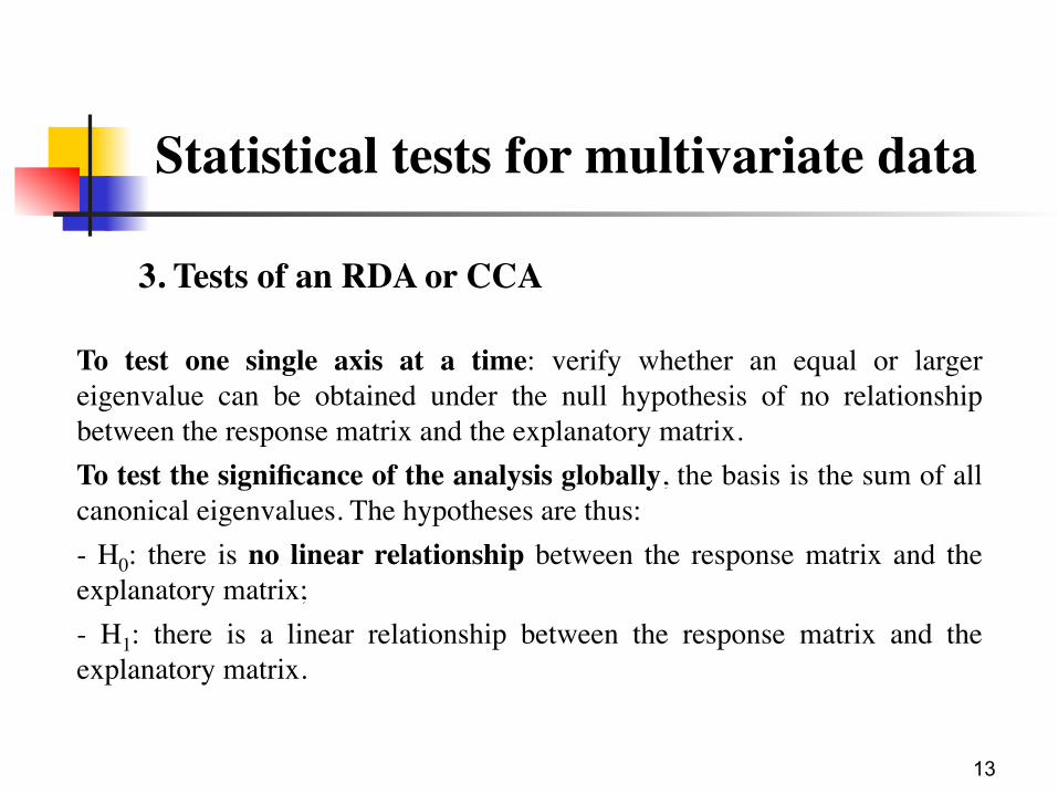
3. Tests of an RDA or CCA
To test one single axis at a time: verify whether an equal or larger eigenvalue can be obtained under the null hypothesis of no relationship between the response matrix and the explanatory matrix. To test the significance of the analysis globally, the basis is the sum of all canonical eigenvalues. The hypotheses are thus:- H0: there is no linear relationship between the response matrix and the explanatory matrix;- H1: there is a linear relationship between the response matrix and the explanatory matrix.
14
Statistical tests for multivariate data
3. Tests of an RDA or CCA
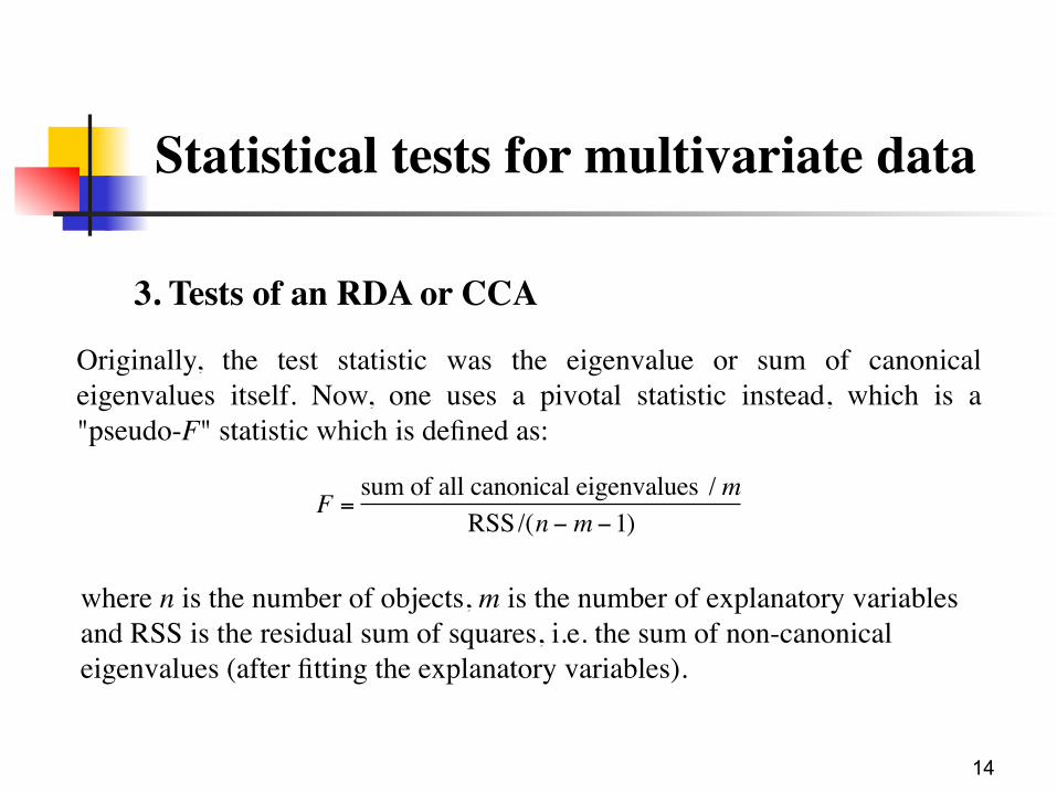
Originally, the test statistic was the eigenvalue or sum of canonical eigenvalues itself. Now, one uses a pivotal statistic instead, which is a "pseudo-F" statistic which is defined as:
F = sum of all canonical eigenvalues / mRSS/(n − m −1)
where n is the number of objects, m is the number of explanatory variables and RSS is the residual sum of squares, i.e. the sum of non-canonical eigenvalues (after fitting the explanatory variables).
15
Statistical tests for multivariate data
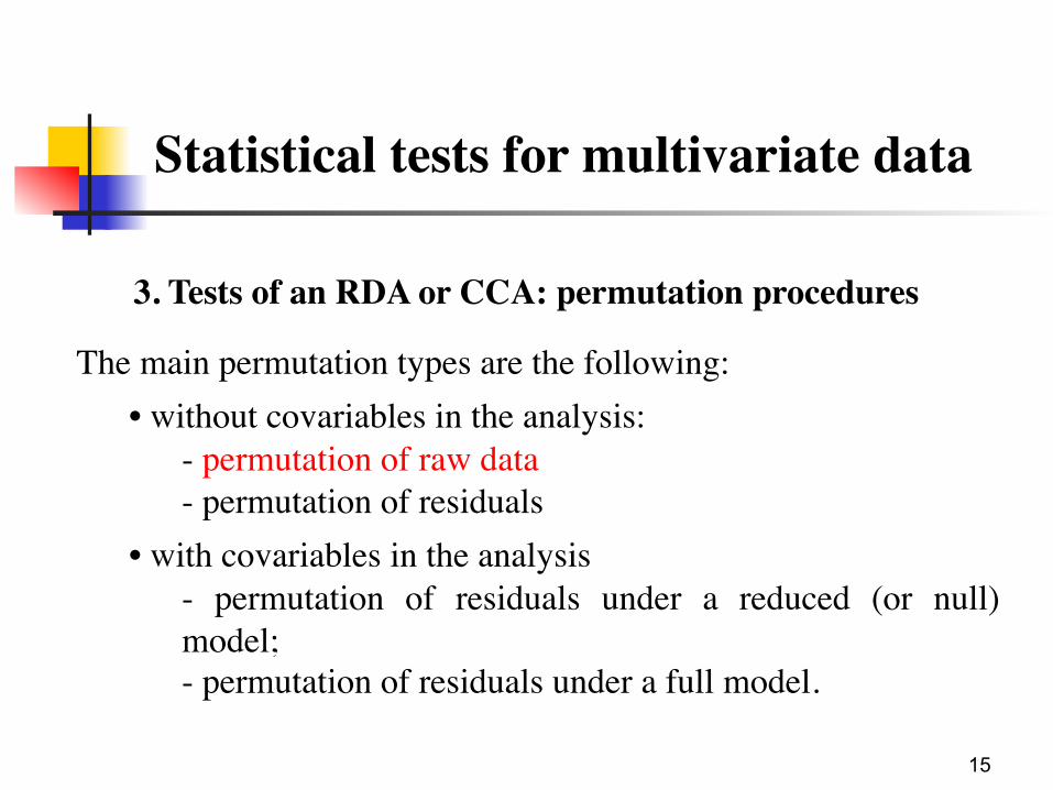
3. Tests of an RDA or CCA: permutation procedures
The main permutation types are the following:• without covariables in the analysis:
- permutation of raw data- permutation of residuals
• with covariables in the analysis- permutation of residuals under a reduced (or null) model;- permutation of residuals under a full model.

16
Day 3
Canonical ordination
17
Canonical ordination
1. Introduction
• Explicitly puts into relationship two matrices: one dependent matrix and one explanatory matrix. Both are involved at the stage of the ordination.
• This approach combines the techniques of ordination and multiple regression
18
Canonical ordination
1. Introduction
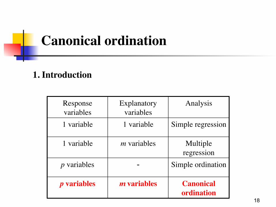
Response variables
Explanatory variables
Analysis
1 variable 1 variable Simple regression
1 variable m variables Multiple regression
p variables - Simple ordination
p variables m variables Canonical ordination
19
Canonical ordination
1. Introduction
• The results of RDA and CCA are presented in the form of biplots or triplots.
• The explanatory variables can be qualitative (the multistate ones are declared as "factor" (vegan) or coded as a series of binary variables (e.g. Canoco), or quantitative.
20
Canonical ordination
1. Introduction
• A qualitative explanatory variable is represented on the bi- or triplot as the centroid of the sites that have the description "1" for that variable ("Centroids for factor constraints" in vegan, "Centroids of environmental variables" in Canoco).
• A quantitative explanatory variable is represented as a vector (the vector apices are given under the name "Biplot scores for constraining variables" in vegan and "Biplot scores of environmental variables" in Canoco).
21
Day 3
Redundancy analysis (RDA)
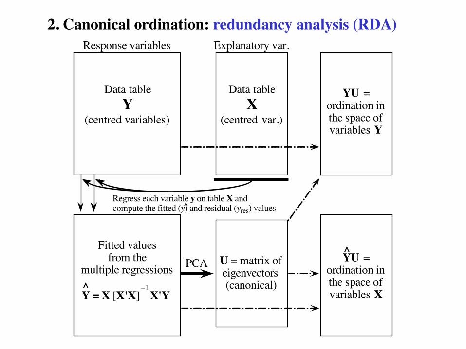
2. Canonical ordination: redundancy analysis (RDA)
Regress each variable y on table X andcompute the fitted (y) and residual (yres) values^
Data tableY
(centred variables)
Response variables
Data tableX
(centred var.)
Explanatory var.
Fitted valuesfrom the
multiple regressions PCA
Y = X [X'X] X'Y^ –1
U = matrix ofeigenvectors(canonical)
YU =ordination inthe space ofvariables X
^
YU =ordination inthe space ofvariables Y
23
Canonical ordination
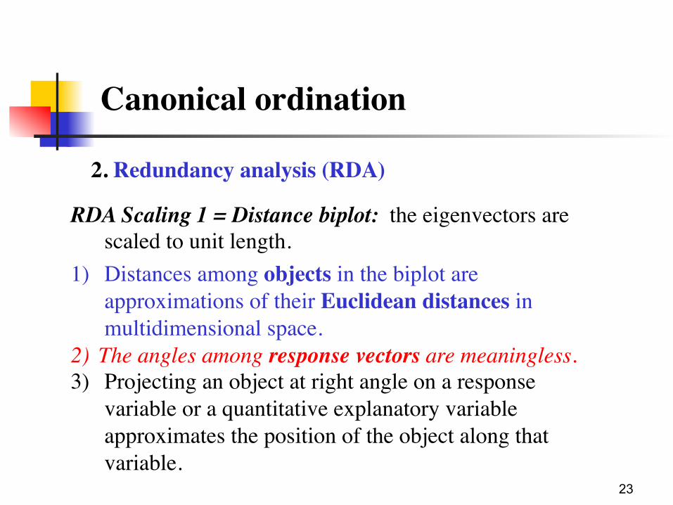
2. Redundancy analysis (RDA)
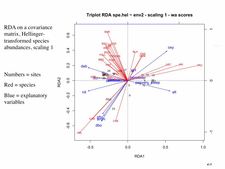
RDA Scaling 1 = Distance biplot: the eigenvectors are scaled to unit length.
1) Distances among objects in the biplot are approximations of their Euclidean distances in multidimensional space.
2) The angles among response vectors are meaningless. 3) Projecting an object at right angle on a response
variable or a quantitative explanatory variable approximates the position of the object along that variable.
24
Canonical ordination
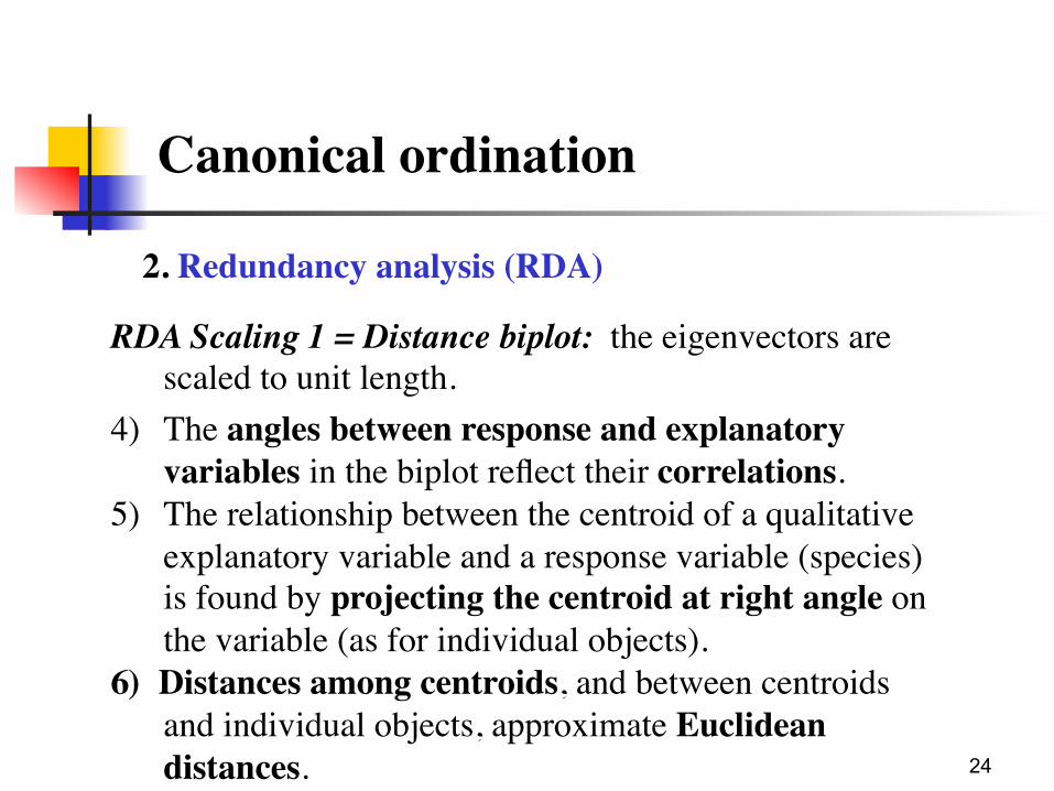
2. Redundancy analysis (RDA)
RDA Scaling 1 = Distance biplot: the eigenvectors are scaled to unit length.
4) The angles between response and explanatory variables in the biplot reflect their correlations.
5) The relationship between the centroid of a qualitative explanatory variable and a response variable (species) is found by projecting the centroid at right angle on the variable (as for individual objects).
6) Distances among centroids, and between centroids and individual objects, approximate Euclidean distances.
25
Canonical ordination
-0.5 0.0 0.5 1.0
-0.6
-0.4
-0.2
0.0
0.2
0.4
0.6
Triplot RDA spe.hel ~ env2 - scaling 1 - wa scores
RDA1
RDA2
CHA
TRUVAILOC
OMB
BLA
HOT
TOX
VAN
CHE
BAR
SPI
GOU BRO
PER
BOU
PSO
ROT
CAR
TAN
BCO
PCH
GRE
GAR
BBO
ABL
ANG
1
234
56 7
9
10
1112
131415
161718
19202122
23
2425
26
2728
2930
alt
deb
pH
dur
pho
nit
amm
oxy
dbo
-10
1
penlowpenmoderatepensteep
penvery_steep
RDA on a covariance matrix, Hellinger-transformed species abundances, scaling 1
Numbers = sites
Red = species
Blue = explanatory variables
26
Canonical ordination
2. Redundancy analysis (RDA)RDA Scaling 2 = correlation biplot: the eigenvectors are
scaled to the square root of their eigenvalue.1) Distances among objects in the biplot are not
approximations of their Euclidean distances in multidimensional space.
2) The angles in the biplot between response and explanatory variables, and between response variables themselves or explanatory variables themselves, reflect their correlations.
3) Projecting an object at right angle on a response or an explanatory variable approximates the value of the object along that variable.
27
Canonical ordination
2. Redundancy analysis (RDA)RDA Scaling 2 = correlation biplot: the eigenvectors are
scaled to the square root of their eigenvalue.4) The angles between descriptors reflect their correlations. 5) The relationship between the centroid of a qualitative
explanatory variable and a response variable (species) is found by projecting the centroid at right angle on the variable (as for individual objects).
6) Distances among centroids, and between centroids and individual objects, do not approximate Euclidean distances.
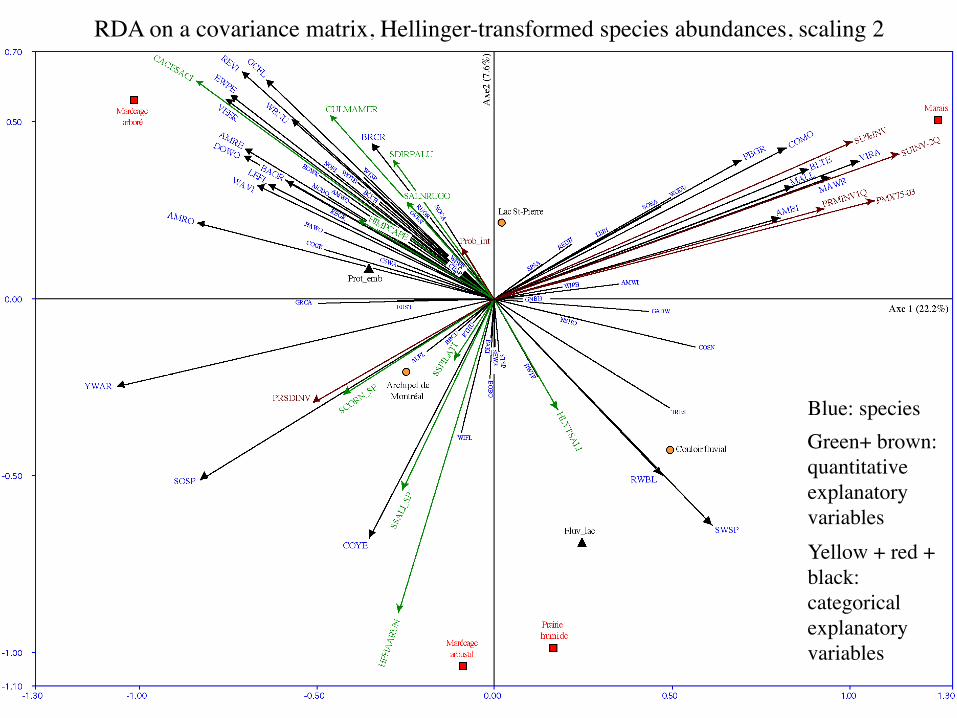
RDA on a covariance matrix, Hellinger-transformed species abundances, scaling 2
Blue: speciesGreen+ brown: quantitative explanatory variablesYellow + red + black: categorical explanatory variables

29
Day 3
Canonical correspondence analysis (CCA)
30
Canonical ordination
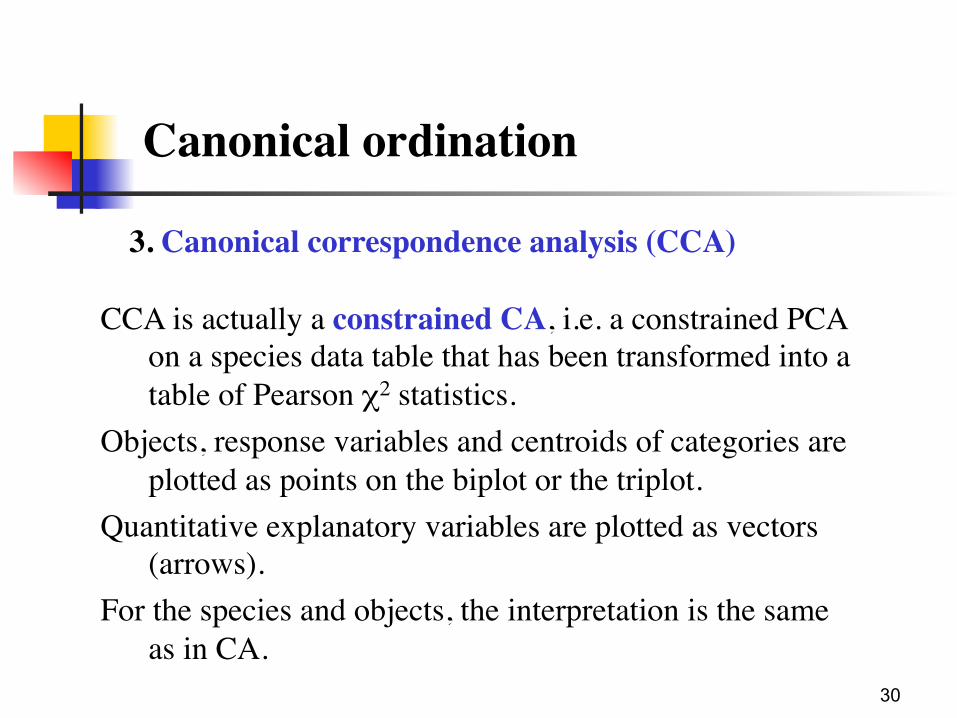
3. Canonical correspondence analysis (CCA)
CCA is actually a constrained CA, i.e. a constrained PCA on a species data table that has been transformed into a table of Pearson χ2 statistics.
Objects, response variables and centroids of categories are plotted as points on the biplot or the triplot.
Quantitative explanatory variables are plotted as vectors (arrows).
For the species and objects, the interpretation is the same as in CA.
31
Canonical ordination
3. Canonical correspondence analysis (CCA)
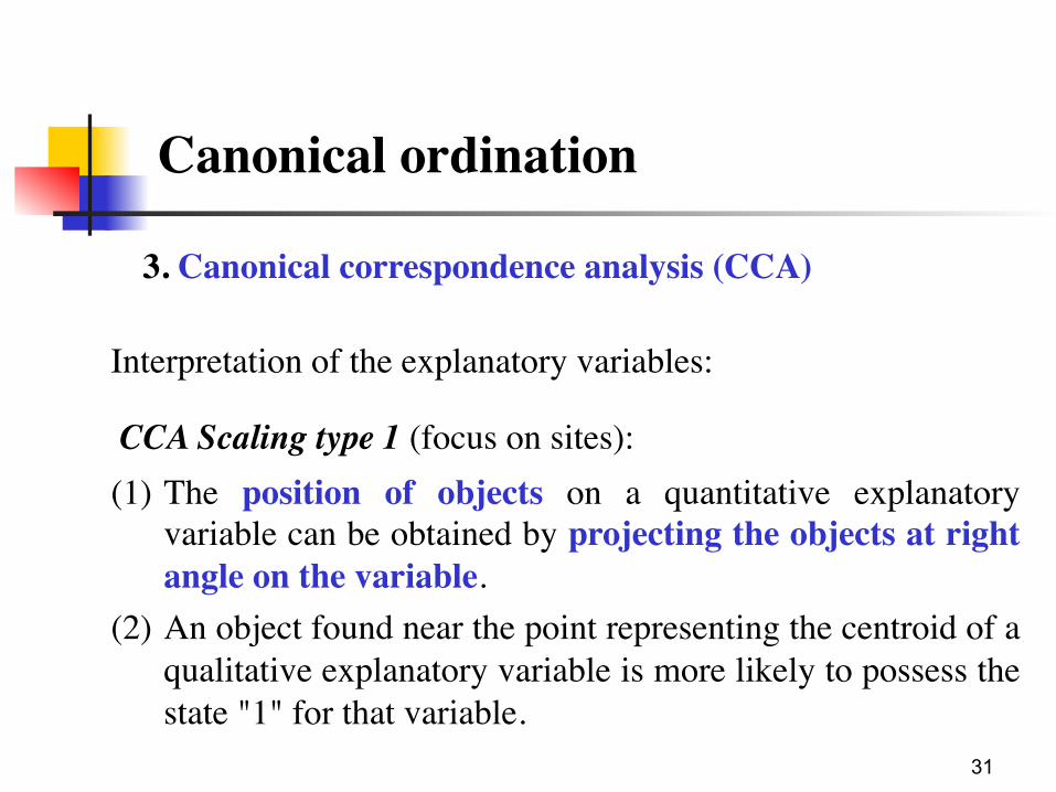
Interpretation of the explanatory variables:
CCA Scaling type 1 (focus on sites): (1) The position of objects on a quantitative explanatory
variable can be obtained by projecting the objects at right angle on the variable.
(2) An object found near the point representing the centroid of a qualitative explanatory variable is more likely to possess the state "1" for that variable.
32
Canonical ordination
3. Canonical correspondence analysis (CCA)
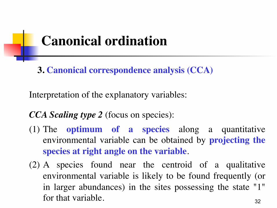
Interpretation of the explanatory variables:
CCA Scaling type 2 (focus on species): (1) The optimum of a species along a quantitative
environmental variable can be obtained by projecting the species at right angle on the variable.
(2) A species found near the centroid of a qualitative environmental variable is likely to be found frequently (or in larger abundances) in the sites possessing the state "1" for that variable.
33
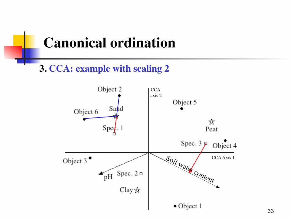
Canonical ordination3. CCA: example with scaling 2
34
Day 3
Multivariate ANOVA by RDA
35
Canonical ordination
4. Multivariate ANOVA by RDA
In its classical, parametric form, multivariate analysis of variance (MANOVA) has stringent conditions of application and restrictions (e.g. multivariate normality of each group of data, homogeneity of the variance-covariance matrices, number of response variables smaller than the number of objects minus the number of groups…).
RDA offers an elegant alternative, and adds the versatility of the permutation tests and the triplot representation of results.
36
Canonical ordination
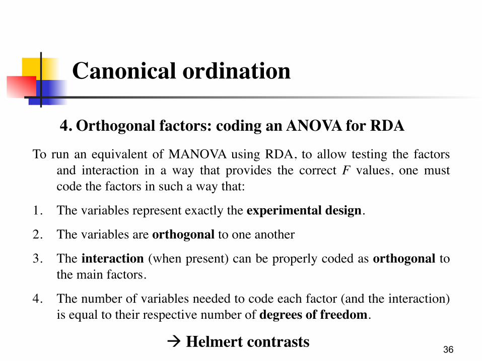
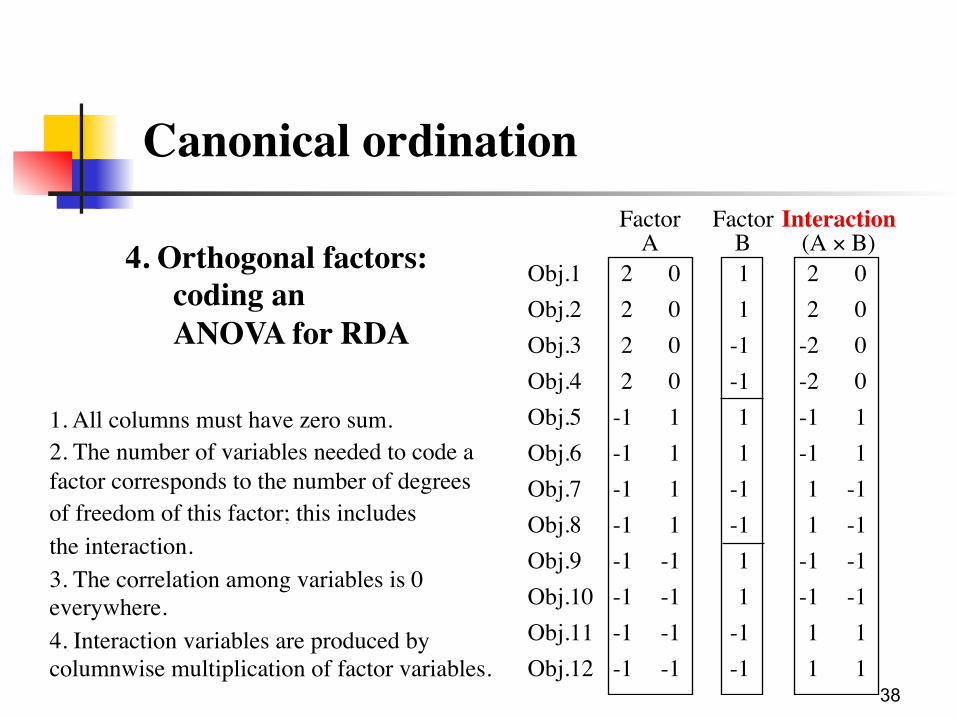
4. Orthogonal factors: coding an ANOVA for RDATo run an equivalent of MANOVA using RDA, to allow testing the factors
and interaction in a way that provides the correct F values, one must code the factors in such a way that:
1. The variables represent exactly the experimental design.
2. The variables are orthogonal to one another
3. The interaction (when present) can be properly coded as orthogonal to the main factors.
4. The number of variables needed to code each factor (and the interaction) is equal to their respective number of degrees of freedom.
à Helmert contrasts
37
Canonical ordination
4. Orthogonal factors: coding an ANOVA for RDA.
Object 1Object 2
Factor B : 2 levels
Fact
or A
: 3 le
vels
n = 12
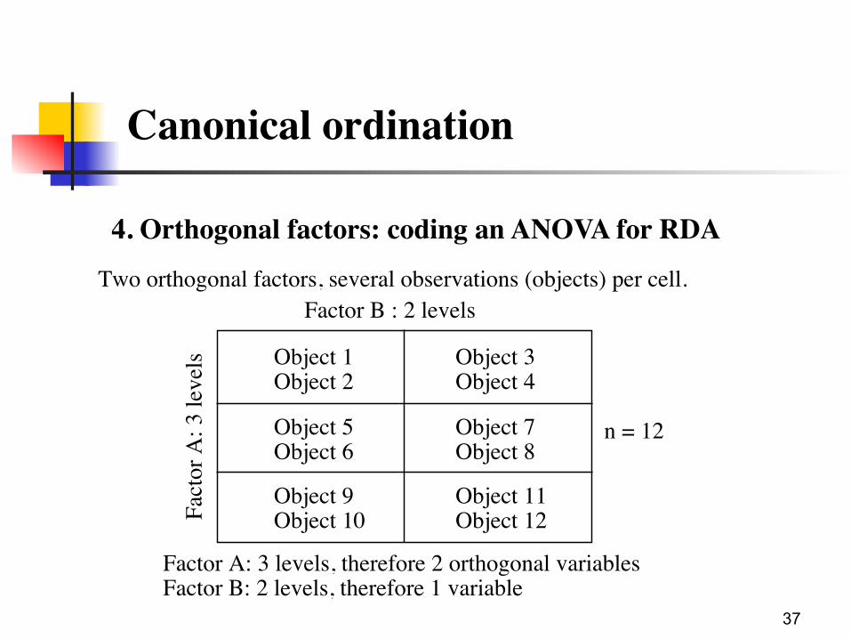
Two orthogonal factors, several observations (objects) per cell.
Object 3Object 4
Object 5Object 6
Object 7Object 8
Object 9Object 10
Object 11Object 12
Factor A: 3 levels, therefore 2 orthogonal variablesFactor B: 2 levels, therefore 1 variable
38
Canonical ordination
4. Orthogonal factors: coding an ANOVA for RDA
2222
-1-1-1-1-1-1-1-1
00001111
-1-1-1-1
11
-1-111
-1-111
-1-1
Obj.1Obj.2Obj.3Obj.4Obj.5Obj.6Obj.7Obj.8Obj.9Obj.10Obj.11Obj.12
FactorA
FactorB
Interaction(A × B)22
-2-2-1-111
-1-111
000011
-1-1-1-111
1. All columns must have zero sum.2. The number of variables needed to code a factor corresponds to the number of degreesof freedom of this factor; this includesthe interaction.3. The correlation among variables is 0 everywhere.4. Interaction variables are produced by columnwise multiplication of factor variables.
39
Canonical ordination
4. Multivariate ANOVA by RDA
WarningTesting by permutations does not alleviate the requirement of homogeneity of within-group dispersions in multivariate ANOVA by RDA.
This condition can be tested in R by function betadisper() {vegan}.
40
Canonical ordination
4. Multivariate ANOVA by RDA
Example27 sites of the (Hellinger-transformed) Doubs fish data and fictitious balanced two-way ANOVA design:
Factor "altitude" (alt.fac): 3 levels
Factor "pH" (pH.fac): 3 levels
41
Canonical ordination
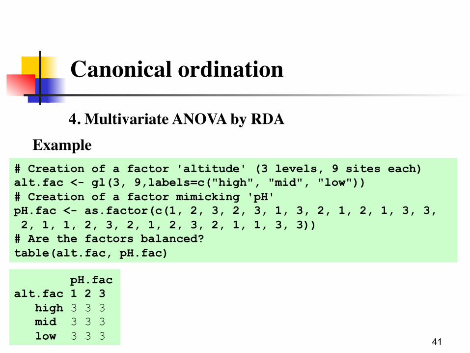
4. Multivariate ANOVA by RDAExample
# Creation of a factor 'altitude' (3 levels, 9 sites each) alt.fac <- gl(3, 9,labels=c("high", "mid", "low")) # Creation of a factor mimicking 'pH' pH.fac <- as.factor(c(1, 2, 3, 2, 3, 1, 3, 2, 1, 2, 1, 3, 3, 2, 1, 1, 2, 3, 2, 1, 2, 3, 2, 1, 1, 3, 3)) # Are the factors balanced? table(alt.fac, pH.fac)
pH.fac alt.fac 1 2 3 high 3 3 3 mid 3 3 3 low 3 3 3
42
Canonical ordination4. Multivariate ANOVA by RDA
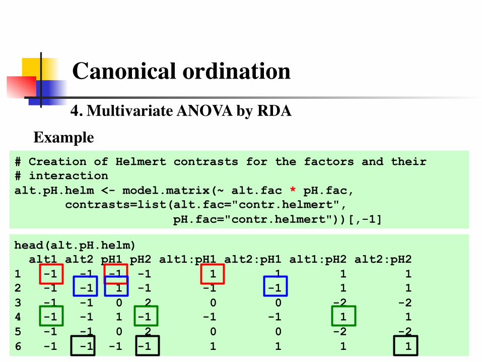
Example# Creation of Helmert contrasts for the factors and their # interaction alt.pH.helm <- model.matrix(~ alt.fac * pH.fac, contrasts=list(alt.fac="contr.helmert", pH.fac="contr.helmert"))[,-1]
head(alt.pH.helm) alt1 alt2 pH1 pH2 alt1:pH1 alt2:pH1 alt1:pH2 alt2:pH2 1 -1 -1 -1 -1 1 1 1 1 2 -1 -1 1 -1 -1 -1 1 1 3 -1 -1 0 2 0 0 -2 -2 4 -1 -1 1 -1 -1 -1 1 1 5 -1 -1 0 2 0 0 -2 -2 6 -1 -1 -1 -1 1 1 1 1
43
Canonical ordination
4. Multivariate ANOVA by RDA
ExampleWithin-group dispersions: see script of today's practicals:
ICTP-Day3.R
Within-group dispersions are homogeneous.
44
Canonical ordination
4. Multivariate ANOVA by RDAExample
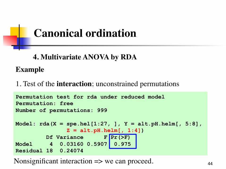
1. Test of the interaction; unconstrained permutationsPermutation test for rda under reduced model Permutation: free Number of permutations: 999 Model: rda(X = spe.hel[1:27, ], Y = alt.pH.helm[, 5:8], Z = alt.pH.helm[, 1:4]) Df Variance F Pr(>F) Model 4 0.03160 0.5907 0.975 Residual 18 0.24074
Nonsignificant interaction => we can proceed.
45
Canonical ordination
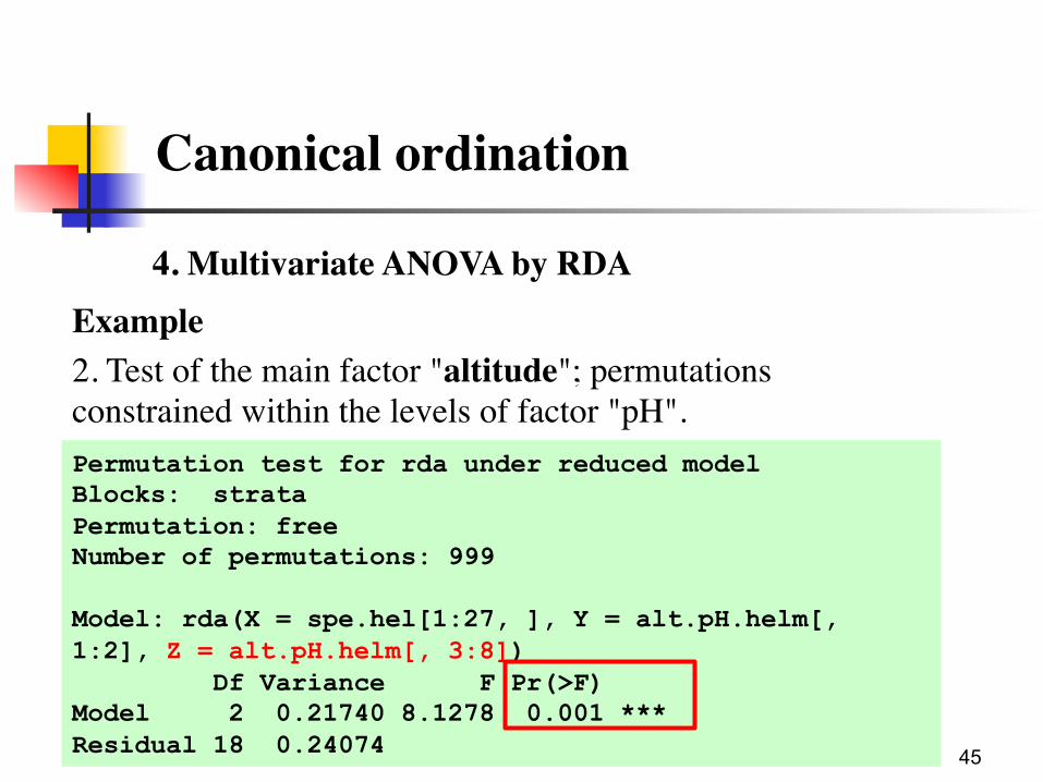
4. Multivariate ANOVA by RDAExample2. Test of the main factor "altitude"; permutations constrained within the levels of factor "pH".Permutation test for rda under reduced model Blocks: strata Permutation: free Number of permutations: 999 Model: rda(X = spe.hel[1:27, ], Y = alt.pH.helm[, 1:2], Z = alt.pH.helm[, 3:8]) Df Variance F Pr(>F) Model 2 0.21740 8.1278 0.001 *** Residual 18 0.24074
46
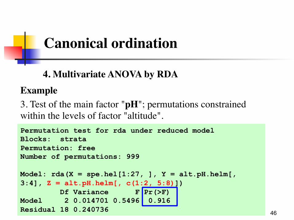
Canonical ordination
4. Multivariate ANOVA by RDAExample3. Test of the main factor "pH"; permutations constrained within the levels of factor "altitude".Permutation test for rda under reduced model Blocks: strata Permutation: free Number of permutations: 999 Model: rda(X = spe.hel[1:27, ], Y = alt.pH.helm[, 3:4], Z = alt.pH.helm[, c(1:2, 5:8)]) Df Variance F Pr(>F) Model 2 0.014701 0.5496 0.916 Residual 18 0.240736
47
Canonical ordination
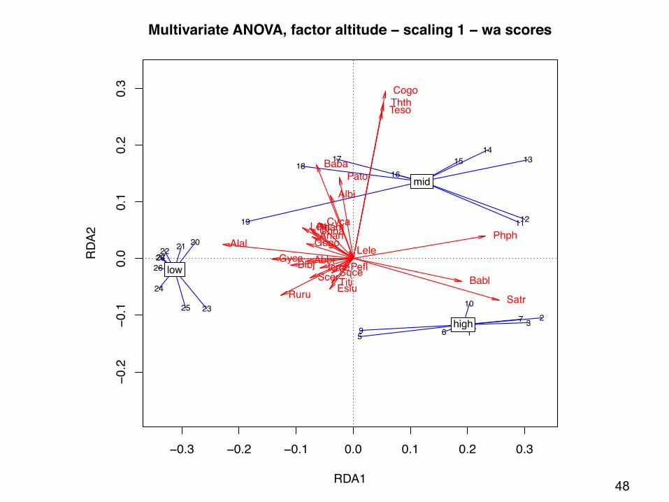
4. Multivariate ANOVA by RDAExample
Only factor "altitude" is significant. One could compute an RDA with the Helmert contrasts coding for altitude, and draw a triplot with the sites' weighted sum scores related to the factor levels, and the arrows of the species scores.
48
Canonical ordination
4. Multivariate ANOVA by RDA
−0.3 −0.2 −0.1 0.0 0.1 0.2 0.3
−0.2
−0.1
0.0
0.1
0.2
0.3
Multivariate ANOVA, factor altitude − scaling 1 − wa scores
RDA1
RDA2
1
2345 6
79
10
1112
1314
1516
1718
19
202122
23
24
25
262728
high
mid
low
Cogo
Satr
Phph
Babl
ThthTeso
Chna
Pato
Lele
Sqce
Baba
Albi
Gogo
Eslu
Pefl
RhamLegi
Scer
Cyca
Titi
AbbrIcmeGyce
Ruru
Blbj
AlalAnan
49
Day 3
Selection of explanatory variables
50
Canonical ordination
5. Selection of environmental variables
There are situations where one wants to reduce the number of explanatory variables in a regression or canonical ordination model for various reasons, e.g.:- not enough "sound ecological thinking => too many candidate explanatory variables;- special procedures (e.g. dbMEM, see Day 5) producing a large number of explanatory variables.
This can be done with a procedure of selection of explanatory variables.
51
Canonical ordination
5. Selection of environmental variables
No single, perfect method exists to reduce the number of variables, besides the examination of all possible subsets of explanatory variables.
In multiple regression, the three usual methods are forward, backward and stepwise selection of explanatory variables, the latter one being a combination of the former two. In RDA, forward selection is the method most often applied.
52
Canonical ordination
The principle of forward selection is as follows:1. Compute, in turn, the independent contribution of each of
the m explanatory variables to the explanation of the variation of the response data table. This is done by running m separate canonical analyses.
2. Test the significance of the contribution of the best variable.3. If it is significant, include it into the model as a first
explanatory variable.
5. Forward selection of environmental variables
53
Canonical ordination
4. Compute (one at a time) the partial contributions (conditional effects) of the m–1 remaining explanatory variables, controlling for the effect of the one already in the model.
5. Test the significance of the best partial contribution among the m–1 variables.
6. If it is significant, include this variable into the model.7. Compute the partial contributions of the m–2 remaining
explanatory variables, controlling for the effect of the two already in the model.
8. The procedure goes on until no more significant partial contribution is found.
5. Forward selection of environmental variables
54
Canonical ordination
a) First of all, forward selection is too liberal (i.e., it allows too many explanatory variables to enter a model).
Before running a forward selection, always perform a global test (including all explanatory variables). If, and only if the global test is significant, run the forward selection.
5. Forward selection of environmental variables
55
Canonical ordination
b) Even if the global test is significant, forward selection is too liberal. Simulations have shown that, in addition to the usual alpha level, one must add a second stopping criterion to forward selection: the model under construction must not have an R2
adj higher than that of the global model (i.e., the model containing all explanatory variables).
5. Forward selection of environmental variables
Blanchet F. G., P. Legendre, and D. Borcard. 2008. Forward selection of explanatory variables. Ecology 89: 2623-2632.
56
Canonical ordination
c) The tests are run by random permutations. d) Like all procedures of selection (forward, backward or
stepwise), this one does not guarantee that the best model is found. From the second step on, the inclusion of variables is conditioned by the nature of the variables that are already in the model.
5. Forward selection of environmental variables
57
Canonical ordination
e) As in all regression models, the presence of strongly intercorrelated explanatory variables renders the regression/canonical coefficients unstable. Forward selection does not necessarily eliminate this problem since even strongly correlated variables may be admitted into a model.
5. Forward selection of environmental variables
58
Canonical ordination
f) Forward selection can help when several candidate explanatory variables are strongly correlated, but the choice has no a priori ecological validity. In this case it is often advisable to eliminate one of the intercorrelated variables on ecological basis rather than on statistical basis.
g) In cases where several correlated explanatory variables are present, without clear a priori reasons to eliminate one or the other, one can examine the variance inflation factors (VIF).
5. Forward selection of environmental variables
59
Canonical ordination
h) The variance inflation factors (VIF) measure how much the variance of the regression or canonical coefficients is inflated by the presence of correlations among explanatory variables. This measures in fact the instability of the regression model.
i) As a rule of thumb, ter Braak recommends that variables that have a VIF larger than 20 be removed from the analysis.
j) Beware: always remove the variables one at a time and recompute the analysis, since the VIF of every variable depends on all the others!
5. Forward selection of environmental variables
60
Canonical ordination
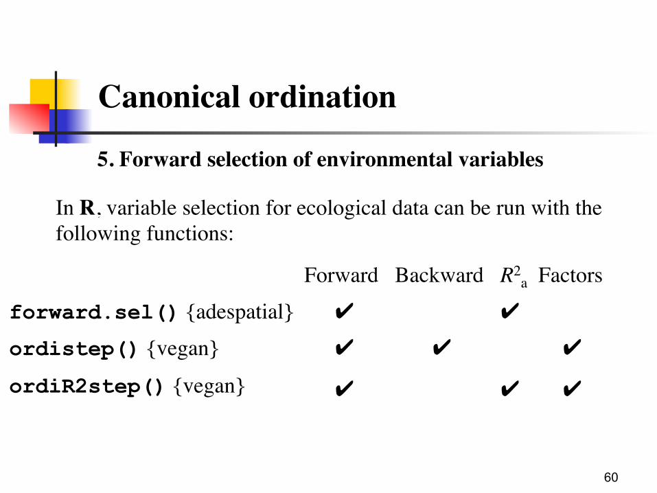
In R, variable selection for ecological data can be run with the following functions:
5. Forward selection of environmental variables
forward.sel() {adespatial}ordistep() {vegan}
ordiR2step() {vegan}
Forward Backward R2a Factors
✔ ✔✔ ✔ ✔
✔ ✔ ✔