i

Analysis of Millimeter Wave FMCW

Radar System for Ranging and Sensing

Applications

A Major Qualifying Project

Submitted to the Faculty of

Worcester Polytechnic Institute

In partial fulfillment of the requirements for the

Degree in Bachelor of Science

in

Physics

By

______________________________________

Jacob Bouchard

Date: 4/25/2019

Project Advisor

______________________________________

Professor Douglas Petkie

This report represents work of WPI undergraduate students submitted to the faculty as evidence of a

degree requirement. WPI routinely publishes these reports on its web site without editorial or peer

review. For more information about the projects program at WPI, see

http://www.wpi.edu/Academics/Projects.

ii

Abstract

For almost a century, work has been proceeding to continuously improve radio detection and

ranging (radar) systems. The development of frequency-modulated continuous-wave radar

(FMCW) systems and the application of millimeter waves, have allowed radar systems to

measure vital signs. No experimental work has been performed to test whether FMCW radar

systems are able to measure displacements on the order of vital signs when multiple moving

targets are in the path of the beam. This paper presents the construction and analysis of an

FMCW radar system operating at a central frequency of 96 GHz being linearly modulated at 10

kHz over a bandwidth of amplitude 96 MHz, culminating in the measurement of two targets

moving with displacements similar to vital sign signatures (~300 μm).

iii

Acknowledgements

I would like to thank my family for their continued support.

I would like to thank Jim Eakin for his invaluable help in the lab

Most importantly I would like to thank my advisor Professor Doug Petkie for his help and insight

and for countless hours spent in and out of the lab working with me.

iv

Table of Contents

Abstract ........................................................................................................................................... ii

Acknowledgements ........................................................................................................................ iii

1. Introduction ................................................................................................................................. 1

1.1 Goal .................................................................................................................................. 2

2. Background ................................................................................................................................. 4

2.1 Radar Systems ....................................................................................................................... 4

2.1.1 Pulsed Radar .................................................................................................................. 4

2.1.2 Continuous-Wave Radar ................................................................................................ 4

2.1.3 Frequency-Modulated Continuous-Wave Radar ........................................................... 5

2.2 Millimeter-Waves for Radar Sensing ................................................................................... 6

2.3 The Michelson Interferometer .............................................................................................. 7

2.4 Lock-In Amplifiers ............................................................................................................... 8

3. Methodology ............................................................................................................................. 10

3.1 Objective 1: Construct the FMCW Radar System .............................................................. 11

3.1.1 Component A: Assemble and Align Components of the System ................................ 12

3.1.2 Component B: Modify Existing Data Collection and Data Analysis Routines ........... 12

3.2 Objective 2: Characterize the Behavior of the System with a Single, Idealized Target ..... 13

3.2.1 Component A: Take Measurements of Large Displacements (~20 mm) to Test the

System and Our Data Analysis Routines .............................................................................. 13

v

3.2.2 Component B: Take Measurements of Small Displacements (~2 mm) to Test the

Resolution of the System ...................................................................................................... 14

3.2.3 Component C: Take Measurements of Displacements on Similar Order of Magnitude

of Vital Signs (~100 μm) ...................................................................................................... 14

3.2.4 Component D: Characterize the Behavior of the Intensity of Different Harmonics at

the Detector Over a Large Range.......................................................................................... 15

3.3 Characterize the Behavior of the System with Two Moving Targets ................................. 15

3.3.1 Measure Two Moving Targets in Different Range Bins Positioned in the Beam ....... 15

4. Findings and Analysis ............................................................................................................... 17

4.1 Single Target Experiments .................................................................................................. 17

4.1.1 Large Displacement Tracking ...................................................................................... 17

4.1.2 Small Displacement Tracking ...................................................................................... 21

4.1.3 Displacements on Similar Order of Magnitude of Vital Signs .................................... 22

4.1.4 Tracking the Behavior of Harmonics Across Range Bins ........................................... 23

4.2 Multiple Target Experiments .............................................................................................. 25

4.2.1 Single Target Moving .................................................................................................. 25

4.2.2 Two Moving Targets.................................................................................................... 26

5 Conclusions and Further Work .................................................................................................. 28

5.1 Conclusions ......................................................................................................................... 28

5.2 Recommendations for Future Work.................................................................................... 28

vi

6 References .................................................................................................................................. 30

Appendix A: System Components ................................................................................................ 33

1

1. Introduction

Since its inception almost a century ago, radio detection and ranging (radar) systems

have been put to use in a variety of important applications [1] from early warning missile

detection systems, and missile guidance systems, to weather detection radars, airport traffic

monitoring and even automatic door openers. Advancements in solid-state technology have

given rise to continuous-wave (CW) frequency-modulated continuous-wave (FMCW) radar that

are being used in automotive applications such as automatic follow distance systems and back-up

obstacle detection. FMCW radar systems send out a continuous wave whose frequency is swept

according to a specific waveform. The reflected signal from the target has embedded information

in the phase and intensity that can be used to determine target’s range, displacement, velocity,

and acceleration. Work has been done to test the feasibility of these systems for the monitoring

of single targets [2] for vital sign signatures at standoff distances (~1-5 m) [3]. Multiple targets

complicate the measurements since the reflected beam contains information about all targets in

the path of the beam. We were interested to see if by using a lock-in detection technique to

measure the harmonics of the modulating beam, we would be able to separate the signals from

each target for the simultaneous monitoring of displacement of several objects.

The use of frequencies between 30 GHz and 300 GHz (the millimeter wave (mmW)

band) in an FMCW radar system have four distinct advantages:

1. The small wavelengths in this band (1 mm-10 mm) should allow very small

movements (~10-100 μm) to be resolved and monitored.

2

2. The shorter wavelengths mean that higher spatial resolution can be realized with

relatively small optical apertures. This can allow for individual targets to be isolated,

or an imaging system to be developed.

3. Transmission through common dielectrics, such as clothing, with sufficient

atmospheric propagation for effective use at distances on the order of ~100 m.

4. With the introduction of 5G and 6G wireless and communication bands on the

horizon, radar transceivers in the millimeter wave band will become more available,

and perhaps be ubiquitous and open up the possibly of a multitude of secondary

applications.

These advantages can allow a mmW radar system to identify individual targets in a cluttered

environment where multiple targets exist. For environments where non-contact vital sign

sensing, such as home health care or military target evaluation, is of interest these advantages

can also be leveraged. The primary purpose of this project is to longitudinally resolve two

moving targets within the same beam or resolution element, which has not been possible using

continuous-wave systems while maintaining the capability to monitor vital signs or other small

displacements or micro-Doppler signatures.

1.1 Goal

The goal of this project is to characterize a mmW FMCW radar system and provide a proof-

of-principle to simultaneously resolve and monitor the displacement of two separate targets. The

project can be broken into two primary objectives:

1. Assemble an FMCW radar and use single moving targets to characterize the system

3

First, an FMCW radar system was built and studied in order to understand its operation and

performance. Measurements were taken of a single moving target across a measurement area of

approximately 3 m. In order to record and process this data custom LabVIEW data acquisition

and IgorPro data analysis programs were designed to characterize the systems performance that

included the incorporation of lock-in detection technique that are key to resolving multiple

targets.

2. Measure two moving targets at two distinct ranges

Once we accurately measured the movement of a single target, we studied how well the system

could measure two distinct moving targets. These two targets would be moving with

displacements on the order of vital signs (~100 μm and frequencies ~1 Hz). This would provide a

proof-of-principle and serve as a foundation to further test the limits of simultaneously

monitoring the displacement of multiple targets over large distances using this technique.

4

2. Background

2.1 Radar Systems

Radio detection and ranging (Radar) systems have been used in a wide variety of

applications for almost a century [1]. At their core, these systems are simply a way to gain

information about a target through its interaction with electromagnetic waves, including its

speed, distance from the antenna, and its identification. There are three primary types of radar

systems and a brief description of each system follows.

2.1.1 Pulsed Radar

Pulsed radar systems were the earliest type of radar systems that were put into practical

use during World War II [4] and are still in use today as weather radars and long range early

warning systems. Pulsed radar systems work by sending out a relatively powerful and short

signal at a target. The system then goes into receiving mode to listen for the pulse that was

reflected off of the target. By measuring the round trip time of flight of the pulse, also called the

running time, the line of sight distance from the radar to the target can be determined by the

equation, 𝛥𝑥 = 𝑐∗𝑡

2 where c is the speed of light and t is the running time [5]. The primary

limitation of pulsed radar systems is that they cannot resolve small displacements due to finite

pulse widths and durations (i.e. ~millimeter displacements correspond to a 6 picosecond change

in the time of flight). This makes them unsuitable for applications such as vital sign sensing.

2.1.2 Continuous-Wave Radar

Continuous wave radar systems utilize a beam consisting of a single, pure carrier

frequency. When this beam hits a target, some of it is reflected back toward the system. This

5

reflected beam has a phase that is different than the emitted beam. This phase change can be used

to monitor the displacement of the target according to the equation 𝛥𝜑 = 2𝜋 ( 2 (𝛥𝑟)

𝜆) where Δr

is the displacement of the target along the beam path and λ is the wavelength of the emitted

beam. This method, or interferometry, allows for the measurement of relatively small

displacements (<100 μm) [6]. Continuous wave radar systems are well suited to applications

where you are only interested in looking at one target. These systems fail when more than one

target is in the emitted beam path. This is due to the fact that if two targets are in the beam path,

the reflected beams from both targets will mix when coming back to the antenna. Extraction, or

deconvolution from a complex superposition of target signatures, of each target can be extremely

difficult and limit the use of a continuous wave radar system in a complex or cluttered

environment.

2.1.3 Frequency-Modulated Continuous-Wave Radar

Frequency-modulated continuous-wave (FMCW) radar systems emit a beam whose

frequency is (typically linearly) modulated over a determined bandwidth. This frequency

modulation gives rise to what are known as range bins. Range bins exist along the path of the

radar beam and have a length (δ) determined by the modulation bandwidth (B) [7], 𝛿 =𝑐

2𝐵.

These range bins correspond to harmonics of the modulation signal. This allows us to “tune” into

harmonics and measure a target in a particular range bin. Due to its similarity to a continuous

wave system, we can also use the phase changes of the reflected wave to track the displacement

of a target within a particular range bin.

6

2.2 Millimeter-Waves for Radar Sensing

Millimeter-waves are electromagnetic waves that have a very high frequency which is

defined as being between 30 GHz and 300 GHz. The short wavelengths of the band (10-1 mm)

allow for small changes in displacement to be monitored (i.e. 1

100 𝜆 ≈ 10 𝜇𝑚). Millimeter-

waves are commonly used in concealed weapons detection as they can easily pass through

common clothing barriers [8]. These two characteristics of millimeter-waves are particularly

attractive for radar applications as it would allow a system to accurately monitor vital signs by

monitoring displacements of the surface of the skin through clothing [9] and are currently a

technology deployed in airports for personnel screening [10]. A large amount of work has also

been done to develop millimeter wave imaging systems [11].

With the 5G and 6G wireless communication revolutions on the horizon, millimeter-wave

sources will be omnipresent in our lives. Telecom giant Verizon began rolling out its 5G service

in the United States, which operates in the 28 GHz range, in 2019 with the first service being

switched on in early April [12]. Researchers in the communication field are predicting that 6G

standardization is not too far off either [13]. These developments in millimeter-wave based

communication has two provides other systems based on millimeter waves two important

advantages. Sources of millimeter-wave radiation will become significantly cheaper, and systems

such as vital sign monitors can easily be integrated into communication networks and into the

Internet of Things (IoT) for sensing applications.

7

2.3 The Michelson Interferometer

The Michelson interferometer was invented by Albert Michelson for use in the famous

Michelson and Morley experiment in 1887 [14]. The interferometer, whose geometry can be

seen in Figure 1, compares the phase of the radiation reflected from the two mirrors where the

phase depends on the path differences.

Figure 1: The geometry of a simple Michelson interferometer showing the source, 50/50 beam splitter, two mirrors, and the

detector [15].

The Michelson interferometer works by emitting electromagnetic radiation from a source,

splitting the radiation equally using a 50/50 beam splitter, reflecting the radiation off of two

mirrors, and recombining the two beams at the detector. For the purposes of this paper, the

intensity of radiation at the detector, as a function of the intensity of the emitted radiation 𝐼0, the

wavelength of the emitted radiation λ, and the optical path difference between the two arms 2x,

where x is the physical path difference in the two arms, can be approximated as

𝐼 ~ 𝐼0 cos (2 𝜋 (2𝑥

𝜆)). We can see that for the case where the emitted beam is of a single

wavelength λ, the intensity goes to zero when the optical path difference is some integer of λ/2.

When used in an FMCW radar system, where the source’s wavelength is varied over a certain

bandwidth, the equation for the Michelson interferometer can be written as

8

𝐼 ~ 𝐼0 cos (2 𝜋 (𝐵

𝑐/2𝑥)) where the substitutions 𝑓 =

𝑐

𝜆 and 𝑓 = 𝐵 where B is the bandwidth of

the linear sweep in the frequency, have been made. When (𝐵

𝑐/2𝑥) is an integer n(i.e. within a

range bin), the intensity signal is a cosine wave with n complete periods as the target is in the

center of a range bin. The number of cycles for a given distance then allows the range of the

target to be identified as in one of the range bins.

2.4 Lock-In Amplifiers

A lock-in amplifier is a tool that is used to detect small AC signals by using phase-

sensitive detection to differentiate the signal from noise or to isolate a particular harmonic of the

modulation frequency (harmonic detection) to improve the signal-to-noise ratio [16]. Phase

sensitive detection works by combining, or multiplying, the input signal with a reference signal,

or a multiple of the reference frequency to identify a harmonic of the fundamental modulation.

Each multiple of the reference frequency corresponds to a target in a particular range bin based

on the ratio (𝐵

𝑐/2𝑥). There are a few different ways to process a signal with a lock-in amplifier but

for the purposes of this project we are only interested in in-phase (I) and quadrature (Q) signals.

I-signals are simply the input signal combined with the reference wave, the Q-signal is the input

signal combined with the reference signal whose phase has been shifted by 90˚. By utilizing I

and Q measurements we were able to process our data more easily as our data analysis routines,

that were developed for a previous continuous wave radar system, were made to process I and Q

signals. These routines would take the raw I and Q signals, box smooth them to eliminate noise

and find the phase. Here the phase is defined as 𝜑(𝑡) = [tan−1 (𝑉𝑄(𝑡)

𝑉𝐼(𝑡))], this phase was

9

discontinuous. To get displacement data from this discontinuous phase, a phase unwrapping

algorithm was applied where 𝜑(𝑡) = 2 π (2 𝑥(𝑡)

𝜆) and the displacement was scaled according to

𝑥(𝑡) = 𝜆

2

𝜑(𝑡)

2 𝜋.

10

3. Methodology

The goal of this project was to construct and characterize an FMCW radar system based

on the Michelson interferometer and simultaneously measure two distinct moving targets with

displacements similar to vital signs (~10-100 μm). To realize our goal, we formalized the

following research objectives:

1. Construct the FMCW radar system.

a. Assemble and align the optical components of the system.

b. Optimize the conditioning electronics (amplifiers and filters) to match the

digitization of the DAQ

c. Develop and modify existing data collection and data analysis routines.

2. Characterize the behavior of the system with a single, idealized target.

a. Take measurements of large displacements (~20 mm > λ) to test the system and

our data analysis routines.

b. Take measurements of small displacements (~2 mm ≈ λ) to test the resolution of

the system.

c. Take measurements of displacements on similar order of magnitude of vital signs

(~100 μm < λ).

d. Characterize the behavior of the intensity of different harmonics at the detector

over a large range.

3. Characterize the behavior of the system with two moving targets.

a. Measure two moving targets in different range bins, with similar but distinct

motions, positioned in the beam.

11

b. Determine if the signatures of the targets interfere in different range bin interfere

with each individual signature.

3.1 Objective 1: Construct the FMCW Radar System

A basic layout of the system is present in Figure 2 with the components listed in

Appendix A.

Figure 2: A simplified layout of the FMCW radar system developed for this project.

For the purposes of this project, the RF signal generator was set at 8 GHz, this signal was

passed through a combined frequency multiplier and emitter, the multiplier upped the signal to

96 GHz (×12) through an active ×4 multiplier and a passive ×3 multiplier with an output power

on the order of 1 mW. The signal was swept as a linear ramp function at 10 kHz over a

bandwidth of amplitude 192 MHz (peak-to-peak deviation), the frequency of the ramp function

12

as was a reference signal for the lock-in amplifier. The detector was a single signal detector; the

signal was passed through a low noise preamplifier set as a bandpass filter between 10 kHz to 1

MHz with a gain of 100. The signal from the preamp was passed to a lock-in amplifier set to take

I and Q measurements, the harmonic of the lock-in amplifier was set to the range bin we were

interested in. From the lock-in, the I and Q signals were passed to a data acquisition card, the

digitization rate of the card was set between 1000-10000 Hz depending on the velocity of the

displacement being measured.

3.1.1 Component A: Assemble and Align Components of the System

In order to safely assemble these components, some of which are very sensitive to

electro-static discharge, care was taken to avoid ESD events and monitor input powers into the

frequency multiplier chain. The components were laid out on an optical table and were roughly

aligned by sight. Two ~6 cm Teflon lenses with ~200 mm focal lengths were used to collimate

the mmWs from the horn (~50 mm aperture) of the source and to match the received mmWs

onto the horn of the detector. A ~15 cm Mylar beam splitter optimized for 50/50 spitting was

used to couple to the reference ~60 mm diameter corner cube reflectors and the target arm. In

order to refine the alignment, various components were moved very slightly in the x, y, and z

directions by hand until the signal at the detector was maximized.

3.1.2 Component B: Modify Existing Data Collection and Data Analysis Routines

As mentioned before, this system was constructed from a previously existing continuous

wave radar system [9] so much of the data collection and data analysis routines could be used

and/or modified for this application. The data collection routine from the previous system, was a

LabVIEW VI that translates the linear stage a certain displacement at a specified velocity.

13

Another VI was created based off of the original VI that allowed us to collect data without

having to translate the linear stage, but instead collected data over a specified time.

The data analysis routine from the previous system was an IgorPRO module that

performed the phase unwrapping algorithm and scaled the displacement. For the purposes of our

investigation, the module was modified to allow us to choose whether or not we removed the DC

offset from our data, and over how many points we smoothed our raw data. This module allowed

us to perform all of these tasks automatically and quickly.

3.2 Objective 2: Characterize the Behavior of the System with a Single,

Idealized Target

Before attempting to measure two moving targets, we wanted to confirm that our system

was able to accurately measure the displacement of a single target.

3.2.1 Component A: Take Measurements of Large Displacements (~20 mm) to

Test the System and Our Data Analysis Routines

In order to test our system and data analysis routines, we wanted to attempt to measure

large displacements (~20 mm) compared to the wavelength of 3.125 mm. To do this we attached

a 6 cm diameter, corner cube retroreflector that would reflect the radiation in back at the incident

angle, to a linear stage and centered it in the beam. Using our custom VI, the stage was translated

20 mm (or larger distances). The data from this test was put through our IgorPro routine. Our

initial results had a very poor signal to noise ratio that made it impossible to differentiate the

position to get velocity. The source of this noise was determined to be the Stanford Research

SR830 lock-in amplifier which introduced a large amount of oscillatory digital noise. Once the

14

amplifier was replaced with the Anfatec USB lockin 250 lock-in amplifier, we confirmed that

our system was indeed working and could measure large displacements. These measurements

were taken in the three range bins that fit on our optical table.

3.2.2 Component B: Take Measurements of Small Displacements (~2 mm) to Test

the Resolution of the System

Once we had confirmed that our system could accurately measure large displacements,

we wanted to confirm that our system had great enough resolution to measure small

displacements (~2 mm) that were on the order of magnitude of the wavelength. To do this, we

followed the same procedure as above but instead of translating the stage 20 mm, we translated it

2 mm. This test was also successful and it should be noted that the number of interference fringes

(or periods) was approximately one period. At this point, the DC offset due to bias voltages can

cause the phase unwrapping algorithms to fail as they assume a zero DC offset.

3.2.3 Component C: Take Measurements of Displacements on Similar Order of

Magnitude of Vital Signs (~100 μm)

Once we were confident that our system could measure displacements on the order of

several millimeters, we wanted to verify that we could measure displacements on the order of

vital signs which are approximately 100 μm. To do this we covered the cone of a 8 cm inch

speaker with tinfoil and drove it with a Pasco signal generator at 1 Hz. This speaker was placed

in the path of the beam and the displacement was measured. We lowered the amplitude of the

speaker’s oscillation to the lowest magnitude that the signal generator would allow. This test

confirmed that our system could measure displacement on the order of vital signs for

subwavelength displacements. While this was not successful on all trial runs, it was successful

15

on a majority of tests. While successful, we feel that further studies are needed and a calibration

procedure may be needed that involves displacement over several wavelengths to ensure the

phase unwrapping algorithm is successful.

3.2.4 Component D: Characterize the Behavior of the Intensity of Different

Harmonics at the Detector Over a Large Range

Before introducing a second reflector into the beam path, we wanted to study how the

intensities of the harmonics varied across the three range bins that fit on our optical table. To do

this a corner cube retroreflector was placed in the beam in slid backward along the length of our

optical table. This test was performed for harmonics 1-5 through range bins 1-3 over a distance

of 2.6 m. Results are shown in section 4.1.4.

3.3 Characterize the Behavior of the System with Two Moving Targets

The key experiment for this project was to determine whether or not it would be possible

to simultaneously measure two moving targets within the beam located in different range bins.

3.3.1 Measure Two Moving Targets in Different Range Bins Positioned in the

Beam

In order to carry out this experiment, two tinfoil covered speakers driven by two separate

function generators were placed in two separate range bins. In order to not completely block out

the beam, the smaller (~5 cm diameter) of the two speakers was placed in range bin two

oscillating at 0.706 Hz. A larger speaker, oscillating at 1.00 Hz was placed on a separate optical

breadboard off of the edge of the optical table that was positioned in range bin four. With both

16

speakers oscillating measurements were taken with the lock-in set to harmonic 2 and harmonic 4.

Results are shown in section 4.2.2.

17

4. Findings and Analysis

This chapter contains the results from our experiments as well as our analysis of these

results. When multiple targets were placed in the beam, we discovered that our system could

detect and resolve multiple moving targets in different range bins. The chapter has been split into

two parts, the single target and multiple target experiments, to differentiate between the tests

being performed.

4.1 Single Target Experiments

This section includes the results from our experiments that involved a single target. These

experiments include large and small displacement tests, as well as an analysis of the interaction

between harmonics 2 and 3.

4.1.1 Large Displacement Tracking

The large displacement experiments were done to confirm that our system was able to

track displacements and that our data analysis routines were working as expected. For this test,

the linear stage was placed in the second range bin and translated backwards 20 mm at 10 mm/s.

The raw I and Q data can be seen in Figure 3. We were primarily concerned with the phase of

our raw signal φ which is defined as 𝜑 = tan−1 (𝑉𝑄

𝑉𝐼). The phase of this signal is seen in Figure

4. This phase is discontinuous and, in order to extract relevant displacement information from the

phase, a phase unwrapping algorithm built into IgorPro was applied to the data to make the phase

a continuous function. The displacement measurement from this experiment can be seen in

Figure 5. Ignoring the acceleration present when the stage begins moving, we assume that the

movement of the stage, and therefore the target, is linear and at a constant velocity. The results of

18

a linear fit performed on the displacement, between 0.2 and 1.8 seconds, can be seen in Figure 6.

The residual reveal an approximately 40 mm deviation from a linear translation, which fall

outside of the specification of the accuracy of the linear stages. However, given all of the

testing, we feel confident that is accurately reproducing the motion of the target. An interesting

observation of the data from tests not presented here involved monitoring the motion of the

retroreflector when the stage stops moving. The retroreflector has a significant mass and we

mounted ~20 cm above the linear stage with standard optical components (optical posts and post

holders). This creates the opportunity for the retroreflector to undergo damped oscillation (i.e.

ring down) whenever the stage came to an abrupt stop. The initial amplitude of these oscillations

(when the mirror was stopped) was on the order of 500 m with a ring down time of 10 seconds.

We feel the deviation, or residuals to the linear fit, are showing the retroreflector ‘oscillating’ at

the end of the ~20 cm post that it is mounted to. In this case, we are actually monitoring the

vibrational dynamics of the optical system that we constructed to test the system. We found no

further explanations for this deviation and plan to reduce the moment arm (height of the optical

post) in future experiments to confirm this assumption

19

Figure 3: The raw I and Q data from the large displacement, single target, test. Note that I (the red wave) and Q (the black wave)

are out of phase by 90˚

Figure 4: The phase of the signal from the large displacement experiment. Note the discontinuous nature of the phase that ranges

from -2π to 2π.

20

Figure 5: The displacement information from the large displacement experiment. Note the acceleration curve present between 0

and 0.1 seconds.

Figure 6: The linear fit of the displacement from the large displacement experiment. The residuals are at the top of the graph.

Note that the residuals are on the order of ~20 μm, these could be due to the movement of the stage.

21

These tests were performed across the length of our optical breadboard (~2.5 m), to

confirm that the results were consistent over a large range. The results of this experiment

confirmed that our system was able to detect and measure displacements and that our data

analysis routine was able correctly interpret the data.

4.1.2 Small Displacement Tracking

Once we had established that our system and data analysis routines could accurately track

and interpret large displacements, we took measurements of small displacement (~2 mm and on

the order of the wavelength) at 1 mm/s. This was to confirm that our system could track

displacements that were smaller than before but still easy to observe. These tests were performed

in the three range bins that fit onto our breadboard. The displacements result from range bin 2 is

presented in Figure 7.

Figure 7: The displacement result from translating the linear stage -2 mm at 1 mm/s. Notice the more pronounced acceleration

profiles.

22

The results from this experiment proved to us that our system and data analysis routines

could track and interpret small displacements (~2 mm). The residuals of a linear fit (seen at the

top of the graph) demonstrates that there were deviations of approximately 40 μm. These

deviations may have been due to a combination of the small translation distance and the

acceleration profile of the linear stage.

4.1.3 Displacements on Similar Order of Magnitude of Vital Signs

Our primary interest for applications of this system is for vital sign monitoring from

multiple targets. Before attempting to measure multiple targets, we wanted to confirm that our

system could measure displacements on the same order of magnitude as vital signs which include

the sub-wavelength region of < 1 mm. To do this we placed a tinfoil covered speaker driven at

0.706 Hz was placed in the second range bin and its motion was measured for 10 seconds. This

displacement measurement can be seen in Figure 8.

23

Figure 8: The displacement of a tinfoil covered speaker oscillating at 0.706Hz. Note that the absolute displacement is 40 μm.

This test confirmed that our system was capable of measuring displacements on the order

of vital signs. Performing a curve fit we found that the frequency was accurately measured as

0.715 Hz and the amplitude was constant.

4.1.4 Tracking the Behavior of Harmonics Across Range Bins

In order to understand how the intensities of different harmonics behave over different

range bins, we measured harmonics 2 and 3 across range bins 1, 2, and 3. A graph of the

intensity of the harmonics versus distance can be seen in Figure 9.

24

Figure 9: A graph of the intensities of harmonic 2 and 3 versus distance. The range bins here have width 750 mm.

We see that both harmonics 2 and 3 have large peaks in the first range bin ~78 cm and,

this is likely caused by strong internal reflections that exist within that range bin between the

optical elements within the system. These reflections quickly die off as the target moves out of

that bin. At the distance 1300 mm, which is in the second range bin, the second harmonic has a

peak in intensity. This peak begins to die at 1500 mm which corresponds to the limit of the

second bin. Harmonic 3 has its peak at around 2100 mm which is within the third bin and begins

to die out at 2250 mm. A key takeaway from this experiment is that the peaks don’t die out

immediately at the limit of the bin, they die out more gradually. This gradual die off and ramp up

of the intensities and coupling between range bins may contribute to cross talk between targets in

separate bins and contribute to uncertainties in simultaneous displacement sensing.

25

4.2 Multiple Target Experiments

Once we understood the performance of our system measuring single targets. We were

ready to measure two targets positioned in the beam.

4.2.1 Single Target Moving

To ensure that having two targets in the beam did not hinder our systems ability to

measure a single moving target, we placed one target in the second range bin and kept it

stationary. We placed another target on a separate optical breadboard off of the optical table

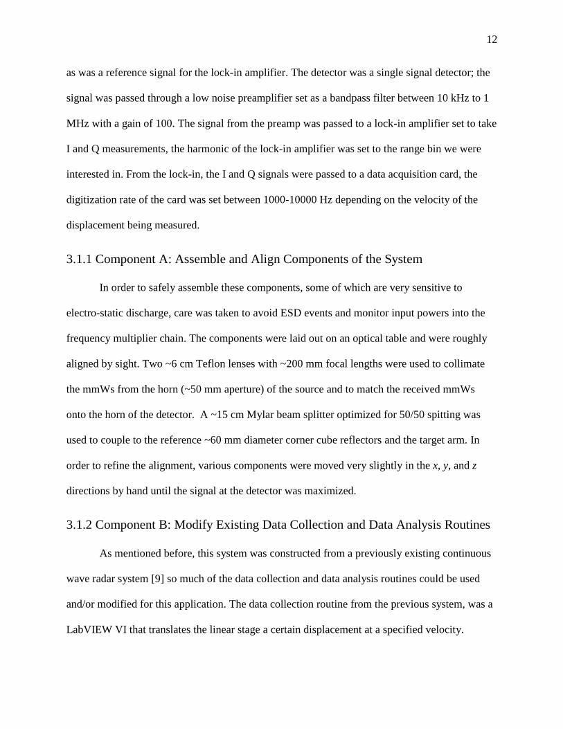
located in the fourth range bin and had it oscillate at 1 Hz. The measurement taken of the fourth

harmonic is in Figure 10.

Figure 10: Displacement measurement taken in the fourth harmonic of a target in the fourth range bin oscillating at 1 Hz. This

measurement was taken when there was a stationary target in the second range bin.

We found that the amplitude of the oscillation was 90 μm. This measurement confirmed

that stationary targets in lower range bins do not affect measurements in higher range bins. This

26

result was very encouraging and allowed us to move onto measurements of multiple moving

targets in different range bins.

4.2.2 Two Moving Targets

Our key experiment in this project was to test if our system could adequately measure

two moving targets in two different range bins. To do this, the target in the second range bin was

set oscillating at 0.706 Hz and the target in the fourth range bin was set oscillating at 1.0 Hz.

Measurements were taken of the second and fourth harmonics to determine the effectiveness of

our system. Measurements from this experiment are seen in Figures 11 and 12.

The measurement of the second harmonic displayed a normal displacement pattern of a

target oscillating at 0.706 Hz. The fourth harmonic shows a displacement pattern of a target

oscillating at 1 Hz, however there is an unexpected modulation of the intensities in bin 4. This

modulation can be seen when comparing the amplitudes of the displacement from this test with

the amplitudes of the displacement in the previous experiment. We expect the amplitudes to be

the same. Since this modulation is not present when the target in the second range bin was

stationary, we can say that it is caused by some interaction between the displacement signals

from bin 2 and 4. We did not observe any significant impact on the measurement in bin 2.

27

Figure 11: Measurement of the second harmonic where there was a target in the second range bin was oscillating at 0.706 Hz

and a target in the fourth range bin was oscillating at 1 Hz.

Figure 12: Measurement of the fourth harmonic where there was a target in the second range bin was oscillating at 0.706 Hz

and a target in the fourth range bin was oscillating at 1 Hz. The dashed lines represent the amplitude of the displacements from

Figure 10.

28

5 Conclusions and Further Work

The objective of this project was to determine whether or not a millimeter wave FMCW

radar system operating at a central frequency of 96 GHz being modulated a frequency of 10 kHz

over a bandwidth of amplitude 96 MHz was capable of measuring the displacements of multiple

targets at different ranges that were on the order of vital signs. Measurements of this type had

never been performed before, to our knowledge, and the applications of such a system are very

exciting.

5.1 Conclusions

We found that our system was able to measure the displacement of multiple targets that

were on the order of vital signs. We discovered that displacements in lower bins has some effect

on the measurements of displacements in higher bins, but not the reverse. This effect is most

likely due to the slow die off of the intensity of harmonics in higher range bins. We were able to

accurately measure the frequency of oscillation for two targets in different range bins. For the

target that was further away, we observed a sort of ‘beat note’ phenomena and the amplitude of

the oscillation (90 μm) oscillated about this value with deviations up to 30 μm. The oscillation of

this distant target had no effect on the measurements of the oscillations of the closest target.

5.2 Recommendations for Future Work

Further work must be done to investigate the interactions between displacements in

different range bins. A problem that we had when trying to study this phenomenon is that we did

not have access to oscillating targets with a consistent radar cross section. The targets that we

29

were using were curved speakers with tinfoil taped onto the cone. This the inconsistent nature in

the surface of these targets made it hard to determine what part of the phenomena that we were

observing came from range bin cross talk or the deformation of our targets surface.

In order to push our system to its fundamental limit of the smallest displacement that it

can measure, we would like reduce all unwanted reflections. These unwanted reflections, usually

from stationary objects in the range bin of interest, tend to overwhelm signals from small

displacements. In order to cancel these reflections, we recommend covering all flat surfaces in

the direction of the beam with eccosorb, a mmW absorbing material.

We would have liked to have made our system mobile so that we could have changed the

environments where we took our measurements. Making the system mobile would also allow us

to take measurements over much larger ranges. In order to mobilize the system, we recommend

moving the system onto a cart. In mobilizing the system, we also recommend replacing the 6 cm

Teflon lenses with larger optics. These larger optics would allow for more targets to be placed in

the path of the beam without completely blocking the beam while increasing the radiation

received with a larger optic.

Through performing this experiment, we formulated an idea for a modified FMCW radar

system that would allow for greater range resolution and more accurate displacement

measurements. This system would employ adaptive waveform, machine learning, cognitive radio

methods to continuously change the size of the range bins. Using this method, the system would

theoretically be able to perfectly measure the displacement of many targets and optimize the

measurement of the displacement of multiple targets in different range bins.

30

6 References

[1] M. I. Skolnik, "Radar," 28 December 2018. [Online]. Available:

https://www.britannica.com/technology/radar/History-of-radar. [Accessed 21 April 2019].

[2] A. Dallinger, S. Schelkshorn and J. Detlefsen, "Broadband Millimeter-wave FMCW Radar

for Imaging of Humans," IEEE, 2006.

[3] D. T. Petkie, E. Bryan, C. Benton and B. D. Rigling, "Millimeter-wave radar systems for

biometric applications," Millimetre Wave and Terahertz Sensors and Technology II, vol.

7485, 2009.

[4] A. Marsh, "From World War II Radar to Microwave Popcorn, the Cavity Magnetron Was

There," 31 October 2018. [Online]. Available: https://spectrum.ieee.org/tech-history/dawn-

of-electronics/from-world-war-ii-radar-to-microwave-popcorn-the-cavity-magnetron-was-

there. [Accessed 21 April 2019].

[5] C. Wolff, "Radar Tutorial," 1998. [Online]. Available:

http://www.radartutorial.eu/02.basics/Pulse%20Radar.en.html. [Accessed 17 April 2019].

[6] J. Tu, T. Hwang and J. Lin, "Respiration Rate Measurement Under 1-D Body Motion

Using Single Continuous-Wave Doppler Radar Vital Sign Detection System," IEEE

TRANSACTIONS ON MICROWAVE THEORY AND TECHNIQUES, vol. 64, no. 6, pp.

1937-1948, 2016.

31

[7] G. M. Brooker, "Understanding Millimetre Wave FMCW Radars," University of Sydney,

Sydney, 2005.

[8] D. M. Sheen, D. L. McMakin and T. E. Hall, "Three-Dimensional Millimeter-Wave

Imaging for Concealed Weapon Detection," IEEE TRANSACTIONS ON MICROWAVE

THEORY AND TECHNIQUES, vol. 49, no. 9, pp. 1581-1592, 2001.

[9] D. T. Petkie, E. Bryan, C. Benton, C. Phelps, J. Yoakum, M. Rogers and A. Reed, "Remote

respiration and heart rate monitoring with millimeter-wave/terahertz radars," Proceedings

of SPIE, vol. 7117, 2008.

[10] L3 Security & Detection Systems, "Advanced Personnel Screening," L3 Security &

Detection Systems, 2019. [Online]. Available:

https://www.sds.l3t.com/products/advancedimagingtech.htm. [Accessed 25 April 2019].

[11] R. Zhang and S. Cao, "3D Imaging Millimeter Wave Circular Synthetic Aperture Radar,"

Sensors, vol. 17, no. 1419, 2017.

[12] C. d. Looper, "Verizon 5G rollout: Here is everything you need to know," 4 April 2019.

[Online]. Available: https://www.digitaltrends.com/mobile/verizon-5g-rollout/. [Accessed

21 April 2019].

[13] E. Schulze, "5G is barely here and some people, not just President Trump, are talking about

6G," 4 March 2019. [Online]. Available: 2019. [Accessed 21 April 2019].

[14] H. D. Young and R. A. Freedman, "35.5 The Michelson Interferometer," in University

Physics with Modern Physics, New York, Pearson Education, 2016, pp. 1176-1178.

32

[15] L. Motta, "Michelson Interferometer," Wolfram Research, 2007. [Online]. Available:

http://scienceworld.wolfram.com/physics/MichelsonInterferometer.html. [Accessed 21

April 2019].

[16] S. R. Systems, About Lock-In Amplifiers, Sunnyvale: Stanford Research Systems.

[17] M. C. Moulton, M. L. Bischoff, C. Benton and D. T. Petkie, "Micro-Doppler radar

signatures of human activity," SPIE Millimetre Wave and Terahertz Sensors and

Technology III, vol. 7837, 2010.

33

Appendix A: System Components

Agilent E8254A, 250 kHz-40 GHz RF signal generator

Virginia Diodes 80-120 GHz, 12 times frequency multiplier chain

BK Precision, DC power supply (used to power the active frequency multiplier)

Mylar 50/50 beam splitter

Custom 2 inch Teflon lenses with 100 mm and 120 mm focal lengths

Newmark Systems NLS4-12-16-1, 12-inch linear stage

Newmark Systems NSC M4, Motor controller

ELVA ZBD-08, 90-140 GHz detector

Stanford Research SR560, Low-noise Preamplifier

Stanford Research SR830, Lock-in amplifier

Anfatec USB LockIn 250, Lock-in amplifier

National Instruments BNC 2110 DAQ, Data acquisition card

Keysight DSOX 1102G, 70MHz oscilloscope