Embed Size (px)
Citation preview
Analysis of Methods to Calculate Air Infiltration for Use in Energy Calculations Master of Science Thesis in the Master’s Programme Structural Engineering and Building Performance Design
AXEL BERGE Department of Civil and Environmental Engineering Division of Division of Building Technology Building Physics CHALMERS UNIVERSITY OF TECHNOLOGY Göteborg, Sweden 2011 Master’s Thesis 2011:16

MASTER’S THESIS 2011:16
Analysis of Methods to Calculate Air Infiltration for Use in Energy Calculations
Master of Science Thesis in the Master’s Programme Structural engineering and Building Performance Design
AXEL BERGE
Department of Civil and Environmental Engineering Division of Division of Building Technology
Building Physics CHALMERS UNIVERSITY OF TECHNOLOGY
Göteborg, Sweden 2011

Analysis of Methods to Calculate Air Infiltration for Use in Energy Calculations
Master of Science Thesis in the Master’s Programme Structural Engineering and Building Performance Design AXEL BERGE
© AXEL BERGE, 2011
Examensarbete / Institutionen för bygg- och miljöteknik, Chalmers tekniska högskola 2011:16 Department of Civil and Environmental Engineering Division of Division of Building Technology Building Physics Chalmers University of Technology SE-412 96 Göteborg Sweden Telephone: + 46 (0)31-772 1000 Cover: Illustration by Axel Berge Chalmers reproservice / Department of Civil and Environmental Engineering Göteborg, Sweden 2011
I
Analysis of Methods to Calculate Air Infiltration for Use in Energy Calculations
Master of Science Thesis in the Master’s Programme Structural Engineering and Building Performance Design AXEL BERGE Department of Civil and Environmental Engineering Division of Building Technology Building Physics Chalmers University of Technology
ABSTRACT
A decrease in energy use is valuable both from an environmental and an economical perspective. Literature shows that an improved airtightness is cost effective with today’s energy prices. This gives incitements to increase the accuracy of the calculation of energy use due to air infiltration, either to get more accurate results earlier in the building process or to make better choices for how to prioritize when retrofitting an old building. A value for the airtightness can be achieved by a pressurization test, but this cannot be done until the house is built, and for large buildings it is often both costly and the results lack in precision. An alternative to a pressurization test is to estimate the airtightness with a statistical model. The aim of this work has been to analyze the possibilities to use a statistical prediction of the airtightness and to compare the statistical predictions to simplifications commonly used by engineers. The work also compares the variation in energy use due to distribution of the leakages to the variation in energy use due to choice of infiltration model. Two foreign statistical models are tested and adjusted to Swedish conditions using a data base of Swedish buildings. These two models, together with a Swedish statistical model, were used to predict the airtightness of a test building with known airtightness. A variation of leakage distributions was simulated for the test building in a numerical simulation software and the worst and best cases were used for further comparisons.
The main conclusion for this study is that the more advanced infiltration models do not perform better than the simpler ones. The energy use depends to a high degree of the leakage distribution, which is seldom known. With large uncertainties the accuracy will be low, independent of the choice of model. Concerning the foreign statistical models, these could not be used without adjustments. Both models overestimated the leakiness of the buildings in the Swedish database. With adjustment, the models could work but they would have to be adjusted against a larger database of Swedish buildings. The one used gave too bad correlation. However, statistical models could probably be used as guidelines for inexperienced modeling engineers, for cases when the airtightness is not known. The Swedish statistical model gave an even bigger deviation than the adjusted foreign models.
Key words: airtightness, air infiltration, energy calculation, energy use, infiltration models, statistical predictions, contam

II
Analys av metoder för att beräkna infiltration för användning i energiberäkningar Examensarbete inom Structural Engineering and Building Performance Design AXEL BERGE Institutionen för bygg- och miljöteknik Avdelningen för Byggnadsteknologi Byggnadsfysik Chalmers tekniska högskola
SAMMANFATTNING
En minskning av energianvändningen är intressant både från ett miljömässigt och ett ekonomiskt perspektiv. Litteraturen visar att en förbättrad lufttäthet är kostnadseffektiv med dagens energipriser. Det ger incitament att öka precisionen i energiberäkningarna på grund av infiltrationen, antingen för att få mer exakta resultat tidigare i byggprocessen eller för att göra bättre val av var man skall lägga fokus när en gammal byggnad renoveras. Man kan få ett värde på lufttätheten genom att provtrycka byggnaden, men det kan inte göras förrän byggnaden är färdigbyggd och för stora byggnader är det både dyrt och resultaten har dålig precision. Ett alternativ till en provtryckning är att uppskatta lufttätheten med en statistisk modell. Målet med den här rapporten var att analysera möjligheterna att använda statistiska uppskattningar av lufttätheten och jämföra resultaten med de förenklingar som redan görs av ingenjörer. Rapporten jämför också variationen i energianvändning på grund av läckagefördelningen med variationen på grund av valet av infiltrationsmodell. Två utländska statistiska modeller är testade och anpassade till svenska omständigheter genom regression mot en databas av svenska hus. Dessa två tillsammans med en svensk modell användes för att förutsäga lufttätheten för en referensbyggnad med känd lufttäthet. Ett antal olika läckagefördelningar simulerades för testbyggnaden i ett numeriskt simuleringsprogram och det värsta och det bästa fallet användes för fortsatta jämförelser.
Den primära slutsatsen i det här arbetet är att de mer avancerade infiltrationsmodellerna inte presterar bättre än de mer förenklade modellerna. Energianvändningen beror till hög grad av läckagefördelningen, som oftast inte är känd. Med stora osäkerheter blir noggrannheten låg, oberoende av val av infiltrationsmodell. För de utländska statistiska modellerna blev slutsatsen att de inte kan användas utan anpassning. För att anpassa modellerna till Svenska förhållanden skulle en större databas behöva användas. Den använda databasen gav för dålig korrelation. Emellertid skulle de statistiska modellerna antagligen kunna användas som riktlinjer för oerfarna energiberäkningsingenjörer, för byggnader där lufttätheten är okänd. Den Svenska statistiska modellen gav till och med större avvikelser än de anpassade utländska modellerna.
Nyckelord: lufttäthet, infiltration, energiberäkningar, energianvändning, infiltrationsmodeller, statistiska modeller, contam
CHALMERS Civil and Environmental Engineering, Master’s Thesis 2011:16 III
Contents ABSTRACT I
SAMMANFATTNING II
CONTENTS III
PREFACE V
NOTATIONS VI
1 INTRODUCTION 1
1.1 Purpose 1
1.2 Method and limitations 2
2 CONSEQUENCES OF AIR LEAKAGES 3
2.1 Energy 3
2.2 Thermal comfort 3
2.3 Moisture protection 4
2.4 Air quality 4
2.5 Acoustics 5
2.6 Fire safety 5
3 THEORY OF AIR MOVEMENT 6
3.1 Basic equations for air movement 6 3.1.1 Calculating single leakage paths 7 3.1.2 Leakages through the whole envelope 9
3.2 Pressure differences 11 3.2.1 Stack effect 12 3.2.2 Wind induced pressure 13 3.2.3 Ventilation 16
3.3 Air movement and energy use 17
4 AIRTIGHTNESS 19
4.1 Codes for airtightness 20
4.2 Measurements by fan pressurization test 20
4.3 Models to predict airtightness in a building 22
5 STATISTICAL MODELS FOR AIRTIGHTNESS PREDICTION 23
5.1 Factors influencing air tightness 23
5.2 Prediction model for residential buildings in USA 25
5.3 Prediction model for residential buildings in Catalonia 30
CHALMERS, Civil and Environmental Engineering, Master’s Thesis 2011:1616 IV
5.4 Prediction model for buildings in Sweden 34
5.5 Conclusions about statistical models 36
6 DIFFERENT METHODS TO CALCULATE ENERGY USE 38
6.1 Questions to engineers 41
6.2 Persily-Kronvall estimation model 41
6.3 LBL Infiltration Model 42
6.4 Sherman Infiltration Estimation Model 44
6.5 ASHARAE enhanced infiltration model 45
6.6 Numerical simulation software 46 6.6.1 Define the zones of the building 47 6.6.2 Define air flow paths 48 6.6.3 Define weather conditions 48 6.6.4 Define simulation parameters 48 6.6.5 Possibilities for more detailed simulations 49
7 ENERGY CALCULATIONS FOR A REFERENCE BUILDING 50
7.1 Description of the reference building 50 7.1.1 Statistical prediction 50 7.1.2 Discussion about weather 51
7.2 The numerical simulation model 54 7.2.1 Simulations to find extreme cases 56 7.2.2 Leakage distribution based on leakage search 58 7.2.3 Simulation of the ventilation 59
7.3 Results from the numerical simulations 60 7.3.1 Finding the extreme cases for leakage distribution 60 7.3.2 The effect of wind and stack 61 7.3.3 Results for the case with ventilation 64
7.4 Results from the infiltration estimation models 66 7.4.1 Persily-Kronvall and Sherman estimation models 66 7.4.2 LBL infiltration model 68 7.4.3 ASHRAE Enhanced infiltration model 70 7.4.4 Summary of calculation results 71
8 CONCLUSIONS 76
9 RECOMMENDATIONS FOR FURTHER STUDIES 78
10 REFERENCES 79
APPENDIX A: Statistical predictions of the permeability for the detached residential building.
APPENDIX B: Calculation of an example of the leakage distribution.

CHALMERS Civil and Environmental Engineering, Master’s Thesis 2011:16 V
Preface In this work, error sources in various infiltration models have been investigated. The aim has been to detect the influence from unknown information on the characteristics of leakages when calculating the energy use.
The report has been carried out at the division of Building Technology, Chalmers University of Technology, Sweden. The work has been supervised by senior lecturer Paula Wahlgren who has been a great support during the work process.
I want to thank the engineers Emma Eliasson, Christian Johansson, Sonja Ritscher, Hans Wetterlund and Peter Ylmén for valuable input to the work. A special thanks to Owe Svensson for providing input data and for giving me the opportunity to participate at a pressurization test.
Göteborg April 2011
Axel Berge
CHALMERS, Civil and Environmental Engineering, Master’s Thesis 2011:1616 VI
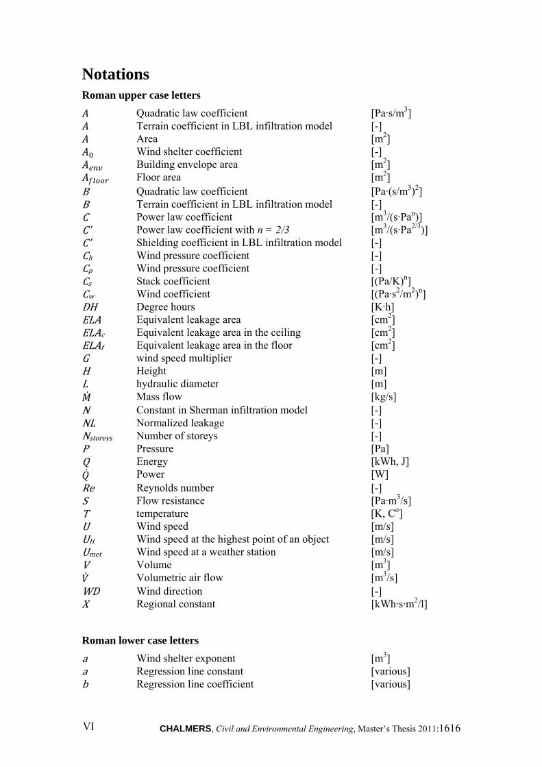
Notations Roman upper case letters
Quadratic law coefficient [Pa·s/m3] Terrain coefficient in LBL infiltration model [-] Area [m2] Wind shelter coefficient [-] Building envelope area [m2] Floor area [m2]
B Quadratic law coefficient [Pa·(s/m3)2] B Terrain coefficient in LBL infiltration model [-] C Power law coefficient [m3/(s·Pan)] C’ Power law coefficient with n = 2/3 [m3/(s·Pa2/3)] C’ Shielding coefficient in LBL infiltration model [-] Ch Wind pressure coefficient [-] Cp Wind pressure coefficient [-] Cs Stack coefficient [(Pa/K)n] Cw Wind coefficient [(Pa·s2/m2)n] DH Degree hours [K·h] ELA Equivalent leakage area [cm2] ELAc Equivalent leakage area in the ceiling [cm2] ELAf Equivalent leakage area in the floor [cm2] G wind speed multiplier [-] H Height [m] L hydraulic diameter [m] Mass flow [kg/s]
N Constant in Sherman infiltration model [-] NL Normalized leakage [-] Nstoreys Number of storeys [-] P Pressure [Pa] Q Energy [kWh, J] Power [W]
Re Reynolds number [-] S Flow resistance [Pa·m3/s] T temperature [K, Co] U Wind speed [m/s] UH Wind speed at the highest point of an object [m/s] Umet Wind speed at a weather station [m/s] V Volume [m3] Volumetric air flow [m3/s]
WD Wind direction [-] X Regional constant [kWh·s·m2/l]
Roman lower case letters
a Wind shelter exponent [m3] a Regression line constant [various] b Regression line coefficient [various]
CHALMERS Civil and Environmental Engineering, Master’s Thesis 2011:16 VII
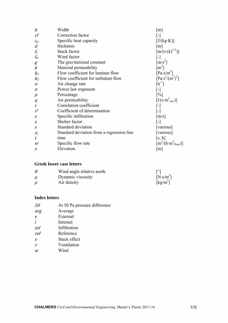
b Width [m] cf Correction factor [-] cp Specific heat capacity [J/(kg·K)] d thickness [m] fs Stack factor [m/(s·(k)1/2)] fw Wind factor [-] g The gravitational constant [m/s2] k Material permeability [m2] k1 Flow coefficient for laminar flow [Pa·s/m3] k2 Flow coefficient for turbulent flow [Pa·s2/(m3)2] n Air change rate [h-1] n Power law exponent [-] p Percentage [%] q Air permeability [l/(s·m2
env)] r Correlation coefficient [-] r2 Coefficient of determination [-] s Specific infiltration [m/s] s Shelter factor [-] s Standard deviation [various] se Standard deviation from a regression line [various] t time [s, h] w Specific flow rate [m3/(h·m3
floor)] z Elevation [m]
Greek lower case letters
θ Wind angle relative north [°] μ Dynamic viscosity [N·s/m2] ρ Air density [kg/m3]
Index letters
50 At 50 Pa pressure difference avg Average e External i Internal inf Infiltration ref Reference
s Stack effect v Ventilation w Wind

CHALMERS, Civil and Environmental Engineering, Master’s Thesis 2011:1616 VIII
CHALMERS, Civil and Environmental Engineering, Master’s Thesis 2011:16 1
1 Introduction Today, when energy prices raise and environmental profiling is an increasingly used marketing argument, the importance of the performance of energy calculations increases accordingly. As the demands on energy savings get stricter the different posts in the energy balance have to be improved. As the walls have grown thicker and the systems for ventilation heat recycling develop, the contribution from air leakages becomes an increasing part of the energy use. A building envelopes resistance to leakage of air is called airtightness. The better the airtightness is the less air flows through the envelope.
Sandberg et al. (2007) concludes that the building owner often will save money with a higher demand on airtightness than what is normally used for Swedish buildings. This creates a need for methods to design a building for good airtightness. Information about the airtightness can also be used to plan what kind of retrofit action to prioritize. To estimate the leakages, the building envelope can be tested with a fan pressurization test. The test is costly, especially for large buildings, and for new buildings it is not possible to do until late in the production phase.
Thus, there is reason to estimate the airtightness with some kind of calculation model instead of measuring it. This would lower costs to evaluate old existing buildings and give a better approximation of the airtightness in the early stages of new projects before the production phase has begun.
There are two different approaches which are possible for the prediction, physical and statistical. In a physical model the building component characteristics are put together into a calculation model with which the leakages can be simulated. A statistical model sets up a combination of variables which can be seen to correlate to the airtightness. With a regression analysis the variables correlation to the airtightness can be estimated and put into the model as correlation parameters. A good statistical model can give a prediction of the tightness but also the standard deviation from the prediction which can be used for a safety margin in the calculation.
As the leakages often are connected to the small scale variation of details, a physical model is problematic to get exact. Therefore the physical model often has to depend on statistical assumptions. The physical models also need large quantities of detailed information. Because of this, there are large benefits which could be gained from a simple statistical model.
Some different statistical models have been created. McWilliams et al. (2006) have made a statistical model from a database of 70 000 American buildings, Montoya et al. (2009) have made a Catalan model based on a database of 251 French buildings and Zou (2010) has made a Swedish model from a database of 185 buildings.
To analyze the possibilities of statistical estimations, knowledge is needed for how large the errors are due to the statistical deviation compared to the errors from simplifications in the handling of the infiltration in the energy calculation.
1.1 Purpose
The aim of this project is to compare different methods to calculate the energy usage due to infiltration. The report will cover the usability of statistical predictions methods to predict the airtightness of a building and the effect on the energy use with respect to how the airtightness is used to calculate the infiltration. The conclusions will be about
CHALMERS, Civil and Environmental Engineering, Master’s Thesis 2011:16 2
how large the errors in the energy calculation are due to which method that is used to calculate the effect of the infiltration. The work will try to answer the following questions:
How is a value for the airtightness achieved today by engineers when the building has not been tested?
Is it possible to use foreign statistical models to predict the airtightness of Swedish buildings?
Does a statistical prediction give significantly better results than the methods used by engineers today?
Does a statistical prediction give good enough results so that it could be possible to use instead of a pressurization test?
How large is the possible variation in the results for calculated energy usage because of an unknown leakage distribution compared to the possible variation in the calculated energy usage due to choice of infiltration model?
1.2 Method and limitations
In order to find out how infiltration is used in the energy calculation among working engineers, five engineers who work with energy calculations at different companies have been contacted. They were also asked about how airtightness is chosen when no pressurization test has been performed.
Three different statistical models have been analyzed; an American model by McWilliams et al. (2006), a Catalan model by Montoya et al. (2010) and a Swedish model by Zou (2010). The American and Catalan models have been used to calculate the airtightness for a database of Swedish buildings. The buildings in the database were detached single family residential houses, they had an even number of floors and all were built the last ten years. Both the actual airtightness and most of the factors used in the statistical models were known for every building. The correlation between the models and the database has been calculated by linear regression with the least square method. This has given correction factors which adjust the models to Swedish conditions.
The error due to deviation from the measured airtightness in the three statistical models and the adjusted versions of the two foreign statistical models has been compared to the errors from other simplifications in the energy calculation. Four different infiltration models have been used to calculate the energy use due to infiltration for a reference building. The reference building was chosen to have a normal airtightness and known information about all the factors used by the statistical models. The reference house was also chosen to be a newly built house since the data base only consisted of newly built houses. The airtightness of the building was also calculated with the statistical models.
The energy use from the calculated infiltration was compared to simulated results in the numerical simulation software CONTAM. In the software the leakage distribution was varied to see how the leakage distribution influenced the energy use. The best case, the worst case and a reference case, based on a partial leakage search of the reference building, were used to compare to the different infiltration models.
CHALMERS, Civil and Environmental Engineering, Master’s Thesis 2011:16 3
2 Consequences of air leakages Air leakages are unintentional openings in the building envelope through which air can pass. The resistance to air flows through the leakages is called the airtightness. The fewer or smaller leakages there are the tighter is the building.
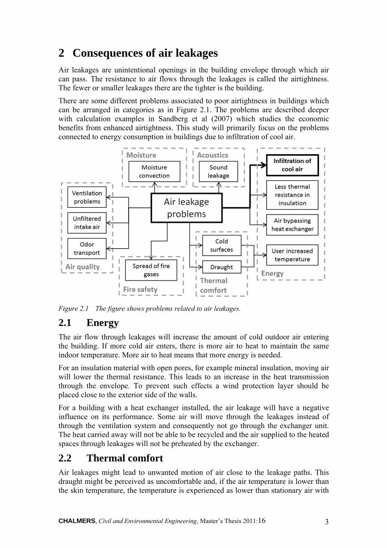
There are some different problems associated to poor airtightness in buildings which can be arranged in categories as in Figure 2.1. The problems are described deeper with calculation examples in Sandberg et al (2007) which studies the economic benefits from enhanced airtightness. This study will primarily focus on the problems connected to energy consumption in buildings due to infiltration of cool air.
Figure 2.1 The figure shows problems related to air leakages.
2.1 Energy The air flow through leakages will increase the amount of cold outdoor air entering the building. If more cold air enters, there is more air to heat to maintain the same indoor temperature. More air to heat means that more energy is needed.
For an insulation material with open pores, for example mineral insulation, moving air will lower the thermal resistance. This leads to an increase in the heat transmission through the envelope. To prevent such effects a wind protection layer should be placed close to the exterior side of the walls.
For a building with a heat exchanger installed, the air leakage will have a negative influence on its performance. Some air will move through the leakages instead of through the ventilation system and consequently not go through the exchanger unit. The heat carried away will not be able to be recycled and the air supplied to the heated spaces through leakages will not be preheated by the exchanger.
2.2 Thermal comfort Air leakages might lead to unwanted motion of air close to the leakage paths. This draught might be perceived as uncomfortable and, if the air temperature is lower than the skin temperature, the temperature is experienced as lower than stationary air with
CHALMERS, Civil and Environmental Engineering, Master’s Thesis 2011:16 4
the same temperature. The moving air might also be cooler than the air in the room and thus lead to local spots of cold air.
If the cold air blows onto indoor surfaces, those will get a lower temperature due to convection. This might be from leakages to the interior spaces or leakages into walls and intermediate floors which will cool the surface materials. Radiation loss to cold surfaces will be perceived as a lower room temperature by the occupants.
The thermal comfort problems can also become an energy problem. Occupants might turn up the indoor heating to compensate for the experienced colder climate due to draught and radiation losses. The magnitude of this effect can be hard to calculate as it depends on a number of factors which are difficult to quantify. For example, user preferences can vary substantially and thus lead to different demands on the indoor climate. How much the leakages affect the occupants depends on how the room is furnished compared to where the leakages are positioned.
2.3 Moisture protection If there is a higher indoor pressure than outdoor pressure, the indoor air can move through leakages to cooler parts of the wall closer to the exterior. As moisture is produced indoors from sources as people, cooking and showering the indoor air will have higher vapor content than the outdoor air. If moist indoor air reaches cooler parts of the walls the relative humidity in these areas will increase. Too high humidity might lead to a variety of biological problems as rot or mould. In the worst case, the relative humidity goes above 100% and then the vapor will condensate and lead to a fast moisture accumulation in the walls.
To prevent this effect an airtight layer is suggested to be put as close to the indoor air as possible. To avoid flow through holes or defects in the airtight layer, the ventilation system could be designed with a larger exhaust flow than the supply flow. This creates an under pressure indoor and the dry outdoor air will move into the building instead of the opposite.
2.4 Air quality When planning a building, the ventilation system is designed to grant a good air quality. Which means that it should be sufficient to replace the indoor air before the quality reaches to low levels. Emissions in the indoor air can either come from within the building or from some site outside of the building.
Contaminants outside of the building can be avoided by installation of filters in the ventilation system or the ventilation orifices. But if the air is infiltrated through air leakages instead, the filters will not be able to remove the pollutants and they will reach into the building.
For indoor emissions, emitted from furniture and occupants and others, the ventilation air flow is dimensioned to exchange the air often enough. In this way the emissions will not reach harmful concentrations. As leakages affect the pressure distribution in and around the building, it will influence the function of the ventilation system and change the ventilation rate. If this leads to a smaller air flow, the air change might be insufficient to cut the concentrations enough to grant the air quality aimed for.
Bad airtightness can also lead to unwanted transport of odors between different parts of the building. For example between apartments or out from the bathroom.
CHALMERS, Civil and Environmental Engineering, Master’s Thesis 2011:16 5
2.5 Acoustics Sound is energy transported as vibrations in air. When the vibration moves from air to a solid material it lose some of its energy and reflects some, the energy which comes out on the other side of the solid will therefore have a lower energy and thus sound less. If there are perforations in the obstacle, the sound will shortcut through these and will not reduce as much as for a completely airtight obstacle. Thus leakages will also affect the disturbance from sound leaking into the building.
2.6 Fire safety A fire transforms solid material to different gas molecules under heat production. This process creates an overpressure both from the increase of gas particles as well as from the increased temperature. The combustion gases can be transported through leakages and thus reach other parts of the building. Aside of the bad smell from the gas it is also toxic and can lead to breathing problems and, if exposed too long, even to brain damage. The hot gas can also spread the actual fire.
CHALMERS, Civil and Environmental Engineering, Master’s Thesis 2011:16 6
3 Theory of air movement Infiltration is the unwanted movement of air through the building envelope. In this chapter theory behind movement of air will be described. The driving forces, the governing equations and some of the simplifications used when calculating air flows in buildings. The effect that the infiltration has on energy use will also be described.
3.1 Basic equations for air movement
The driving force for air movement is pressure. Air moves from a higher pressure to a lower pressure. The total air leakage through a building envelope is built up by the sum of all leakages through holes and cracks in the airtight layer. There are a number of validated models for the leakage through well defined leakage paths; some of which are explained later in this chapter. The problem for a real building is that the quantity and appearance of the leakages are often hard to estimate as the aim is not to have any leakages at all.
To test and model the total leakage through a building, a simplified model can be used. The basic relation between pressure and air flow through ducts or cavities is seen in Equation (3.1) for laminar flow and in Equation (3.2) for turbulent flow. At inlets, outlets and bends on the duct, the air often behave as in Equation (3.2).
∆ (3.1)
∆ (3.2)
where ∆ isthepressuredifference Pa isaconstant Pa ∙ s/m isaconstant Pa ∙ s / m isthevolumeairflow [m3/s]
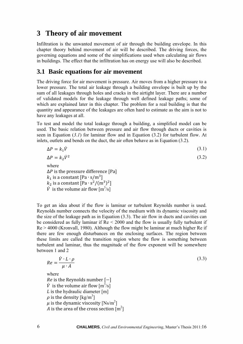
To get an idea about if the flow is laminar or turbulent Reynolds number is used. Reynolds number connects the velocity of the medium with its dynamic viscosity and the size of the leakage path as in Equation (3.3). The air flow in ducts and cavities can be considered as fully laminar if Re < 2000 and the flow is usually fully turbulent if Re > 4000 (Kronvall, 1980). Although the flow might be laminar at much higher Re if there are few enough disturbances on the enclosing surfaces. The region between these limits are called the transition region where the flow is something between turbulent and laminar, thus the magnitude of the flow exponent will be somewhere between 1 and 2
∙ ∙∙
(3.3)
where istheReynoldsnumber isthevolumeairflow [m3/s] isthehydraulic diameter [m] isthedensity [kg/m3] isthedynamicviscosity [Ns/m2]
isthearea ofthecrosssection [m2]
CHALMERS, Civil and Environmental Engineering, Master’s Thesis 2011:16 7
3.1.1 Calculating single leakage paths
There are a number of mathematical models describing the air flow through well-defined leakage paths. Kronvall (1980) created a model to combine different leakages in networks of connected flow resistances, from the basic idea that parallel leakages will have the same pressure difference and leakages connected in series will have the same air flow. The connection between the air flow and the flow resistance is shown in Equation (3.4).
∆
(3.4)
where
is the volumetric air flow[m3/s] ∆ is the pressure difference over the material [Pa]
is the flow resistance [Pa·m3/s]
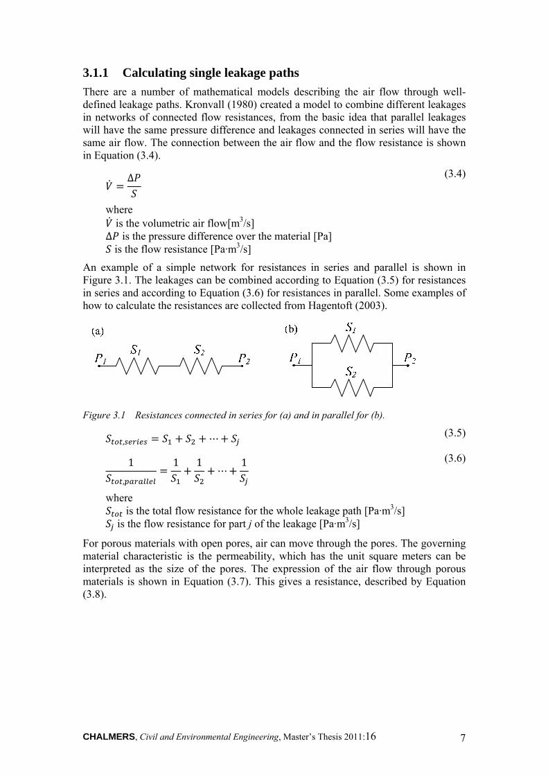
An example of a simple network for resistances in series and parallel is shown in Figure 3.1. The leakages can be combined according to Equation (3.5) for resistances in series and according to Equation (3.6) for resistances in parallel. Some examples of how to calculate the resistances are collected from Hagentoft (2003).
Figure 3.1 Resistances connected in series for (a) and in parallel for (b).
, ⋯ (3.5)
1
,
1 1⋯
1
(3.6)
where
is the total flow resistance for the whole leakage path [Pa·m3/s] is the flow resistance for part j of the leakage [Pa·m3/s]
For porous materials with open pores, air can move through the pores. The governing material characteristic is the permeability, which has the unit square meters can be interpreted as the size of the pores. The expression of the air flow through porous materials is shown in Equation (3.7). This gives a resistance, described by Equation (3.8).
CHALMERS, Civil and Environmental Engineering, Master’s Thesis 2011:16 8
∆
(3.7)
∙∙
(3.8)
where
is the volumetric air flow [m3/s] is the surface area of the material [m2] is the permeability [m2] is the dynamic viscosity [Ns/m2] ∆ is the pressure difference over the material [Pa]
is the thickness of the material [m] is the flow resistance [Pa·m3/s]
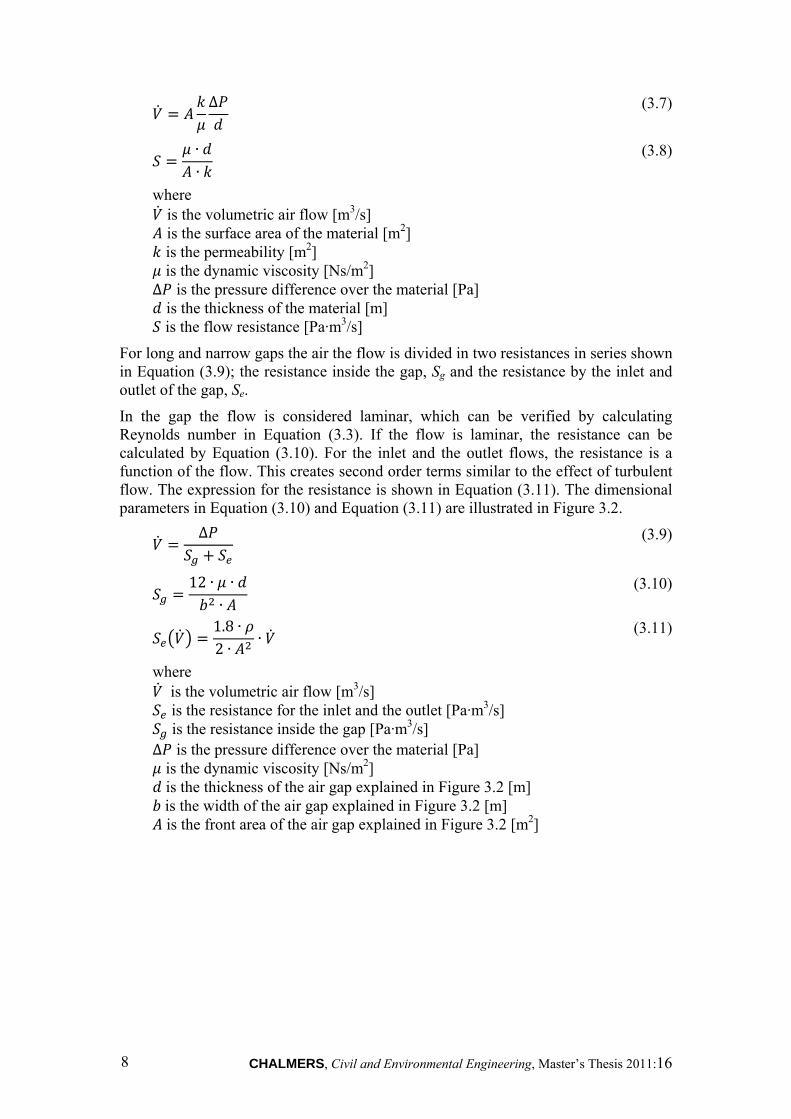
For long and narrow gaps the air the flow is divided in two resistances in series shown in Equation (3.9); the resistance inside the gap, Sg and the resistance by the inlet and outlet of the gap, Se.
In the gap the flow is considered laminar, which can be verified by calculating Reynolds number in Equation (3.3). If the flow is laminar, the resistance can be calculated by Equation (3.10). For the inlet and the outlet flows, the resistance is a function of the flow. This creates second order terms similar to the effect of turbulent flow. The expression for the resistance is shown in Equation (3.11). The dimensional parameters in Equation (3.10) and Equation (3.11) are illustrated in Figure 3.2.
∆
(3.9)
12 ∙ ∙∙
(3.10)
1.8 ∙2 ∙
∙ (3.11)
where is the volumetric air flow [m3/s] is the resistance for the inlet and the outlet [Pa·m3/s] is the resistance inside the gap [Pa·m3/s]
∆ is the pressure difference over the material [Pa] is the dynamic viscosity [Ns/m2] is the thickness of the air gap explained in Figure 3.2 [m] is the width of the air gap explained in Figure 3.2 [m] is the front area of the air gap explained in Figure 3.2 [m2]
CHALMERS, Civil and Environmental Engineering, Master’s Thesis 2011:16 9
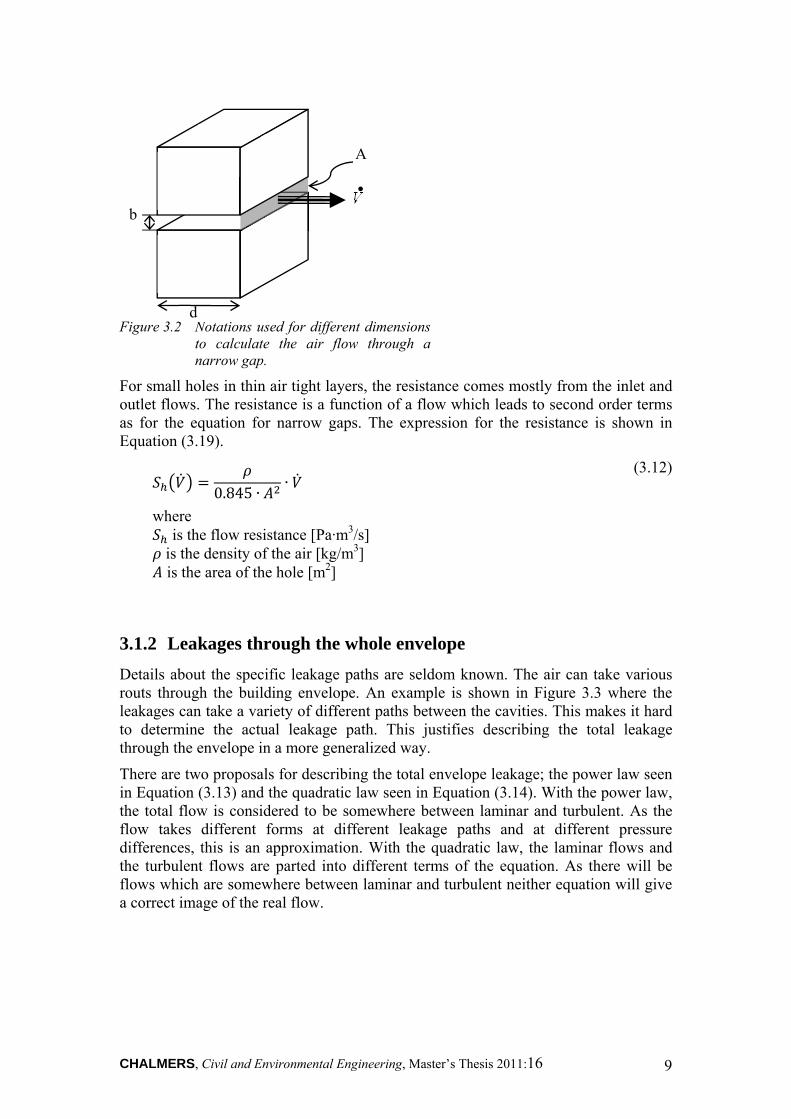
Figure 3.2 Notations used for different dimensions
to calculate the air flow through a narrow gap.
For small holes in thin air tight layers, the resistance comes mostly from the inlet and outlet flows. The resistance is a function of a flow which leads to second order terms as for the equation for narrow gaps. The expression for the resistance is shown in Equation (3.19).
0.845 ∙
∙ (3.12)
where
is the flow resistance [Pa·m3/s] is the density of the air [kg/m3] is the area of the hole [m2]
3.1.2 Leakages through the whole envelope
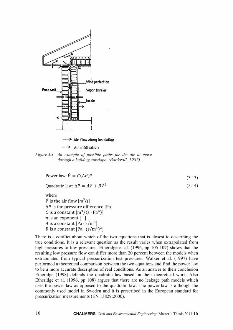
Details about the specific leakage paths are seldom known. The air can take various routs through the building envelope. An example is shown in Figure 3.3 where the leakages can take a variety of different paths between the cavities. This makes it hard to determine the actual leakage path. This justifies describing the total leakage through the envelope in a more generalized way.
There are two proposals for describing the total envelope leakage; the power law seen in Equation (3.13) and the quadratic law seen in Equation (3.14). With the power law, the total flow is considered to be somewhere between laminar and turbulent. As the flow takes different forms at different leakage paths and at different pressure differences, this is an approximation. With the quadratic law, the laminar flows and the turbulent flows are parted into different terms of the equation. As there will be flows which are somewhere between laminar and turbulent neither equation will give a correct image of the real flow.
d
b V .
A
CHALMERS, Civil and Environmental Engineering, Master’s Thesis 2011:16 10
Figure 3.3 An example of possible paths for the air to move
through a building envelope. (Bankvall, 1987)
Power law: ∆ (3.13)
Quadratic law: ∆ (3.14)
where istheairflow [m3/s]
∆ isthepressuredifference Pa isaconstant m / s ∙ Pa isanexponent isaconstant Pa ∙ s/m isaconstant Pa ∙ s/m
There is a conflict about which of the two equations that is closest to describing the true conditions. It is a relevant question as the result varies when extrapolated from high pressures to low pressures. Etheridge et al. (1996, pp 105-107) shows that the resulting low pressure flow can differ more than 20 percent between the models when extrapolated from typical pressurization test pressures. Walker et al. (1997) have performed a theoretical comparison between the two equations and find the power law to be a more accurate description of real conditions. As an answer to their conclusion Etheridge (1998) defends the quadratic law based on their theoretical work. Also Etheridge et al. (1996, pp 108) argues that there are no leakage path models which uses the power law as opposed to the quadratic law. The power law is although the commonly used model in Sweden and it is prescribed in the European standard for pressurization measurements (EN 13829:2000).
CHALMERS, Civil and Environmental Engineering, Master’s Thesis 2011:16 11
These whole envelope models can be used to calculate the flow for one external and one internal pressure but normally the pressure varies over the building envelope which will be explained in the next chapter. To have equilibrium in the system the mass flow into the system must be equal to the mass flow out of the system. Otherwise the system will accumulate or disperse of air. This rule is called the law of mass conservation and is shown in Equation (3.15) and Equation (3.16).
0 (3.15)
∙ (3.16)
where isthemassflowintothe building, through flow path i m s⁄ isthevolumeflowintothe building, through flow path i m s⁄ isthedensityoftheairthrough flow path i kg m⁄
3.2 Pressure differences
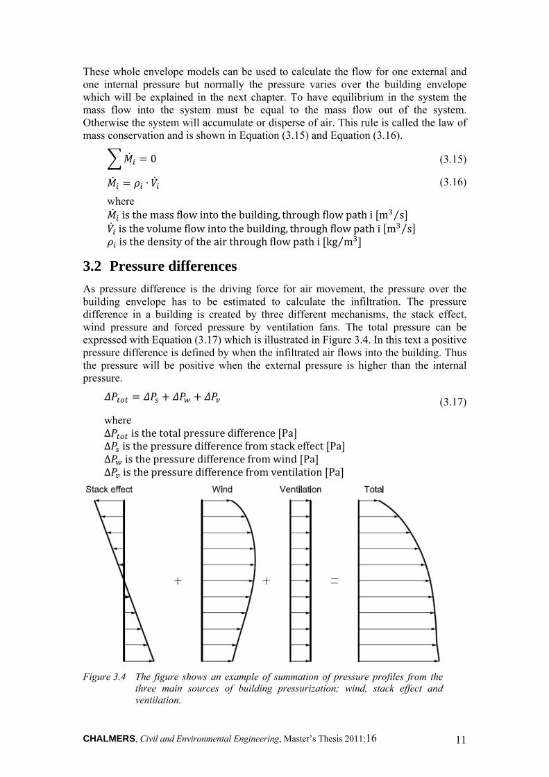
As pressure difference is the driving force for air movement, the pressure over the building envelope has to be estimated to calculate the infiltration. The pressure difference in a building is created by three different mechanisms, the stack effect, wind pressure and forced pressure by ventilation fans. The total pressure can be expressed with Equation (3.17) which is illustrated in Figure 3.4. In this text a positive pressure difference is defined by when the infiltrated air flows into the building. Thus the pressure will be positive when the external pressure is higher than the internal pressure.
(3.17)
where ∆ isthetotalpressuredifference Pa ∆ isthepressuredifferencefromstackeffect Pa ∆ isthepressuredifference from wind Pa ∆ isthepressuredifference from ventilation Pa
Figure 3.4 The figure shows an example of summation of pressure profiles from the
three main sources of building pressurization; wind, stack effect and ventilation.
CHALMERS, Civil and Environmental Engineering, Master’s Thesis 2011:16 12
3.2.1 Stack effect
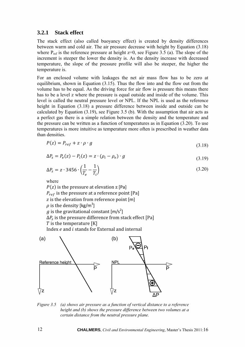
The stack effect (also called buoyancy effect) is created by density differences between warm and cold air. The air pressure decrease with height by Equation (3.18) where Pref is the reference pressure at height z=0, see Figure 3.5 (a). The slope of the increment is steeper the lower the density is. As the density increase with decreased temperature, the slope of the pressure profile will also be steeper, the higher the temperature is.
For an enclosed volume with leakages the net air mass flow has to be zero at equilibrium, shown in Equation (3.15). Thus the flow into and the flow out from the volume has to be equal. As the driving force for air flow is pressure this means there has to be a level z where the pressure is equal outside and inside of the volume. This level is called the neutral pressure level or NPL. If the NPL is used as the reference height in Equation (3.18) a pressure difference between inside and outside can be calculated by Equation (3.19), see Figure 3.5 (b). With the assumption that air acts as a perfect gas there is a simple relation between the density and the temperature and the pressure can be written as a function of temperatures as in Equation (3.20). To use temperatures is more intuitive as temperature more often is prescribed in weather data than densities.
∙ ∙ (3.18)
∆ ∙ ∙ (3.19)
∆ ∙ 3456 ∙
1 1 (3.20)
where isthepressureatelevation z [Pa] isthepressureatareferencepoint Pa
istheelevationfromreferencepoint [m] isthedensity [kg/m3] isthegravitationalconstant [m/s2]
∆ isthepressuredifferencefromstackeffect Pa isthetemperature K Index and standsforExternal and internal
Figure 3.5 (a) shows air pressure as a function of vertical distance to a reference
height and (b) shows the pressure difference between two volumes at a certain distance from the neutral pressure plane.
CHALMERS, Civil and Environmental Engineering, Master’s Thesis 2011:16 13
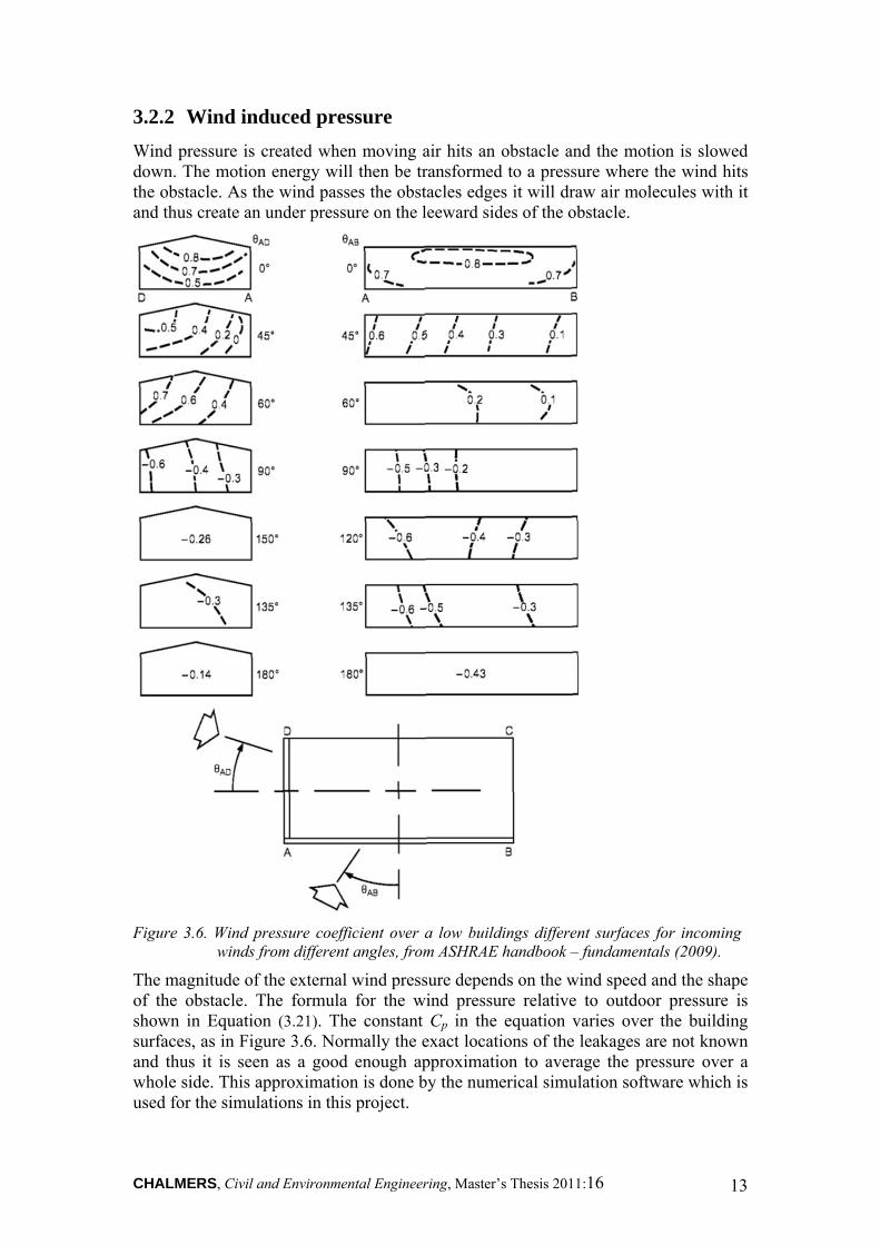
3.2.2 Wind induced pressure
Wind pressure is created when moving air hits an obstacle and the motion is slowed down. The motion energy will then be transformed to a pressure where the wind hits the obstacle. As the wind passes the obstacles edges it will draw air molecules with it and thus create an under pressure on the leeward sides of the obstacle.
Figure 3.6. Wind pressure coefficient over a low buildings different surfaces for incoming
winds from different angles, from ASHRAE handbook – fundamentals (2009).
The magnitude of the external wind pressure depends on the wind speed and the shape of the obstacle. The formula for the wind pressure relative to outdoor pressure is shown in Equation (3.21). The constant Cp in the equation varies over the building surfaces, as in Figure 3.6. Normally the exact locations of the leakages are not known and thus it is seen as a good enough approximation to average the pressure over a whole side. This approximation is done by the numerical simulation software which is used for the simulations in this project.
CHALMERS, Civil and Environmental Engineering, Master’s Thesis 2011:16 14
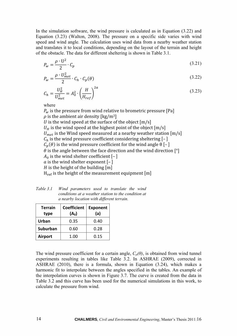
In the simulation software, the wind pressure is calculated as in Equation (3.22) and Equation (3.23) (Walton, 2008). The pressure on a specific side varies with wind speed and wind angle. The calculation uses wind data from a nearby weather station and translates it to local conditions, depending on the layout of the terrain and height of the obstacle. The data for different sheltering is shown in Table 3.1.
∙ U2
∙ (3.21)
∙2
∙ ∙ (3.22)
∙
(3.23)
where isthepressurefromwind relative to brometric pressure Pa istheambientairdensity[kg/m3] isthewindspeedatthesurfaceoftheobject m/s isthewindspeedatthehighestpointoftheobject m/s istheWindspeedmeasuredatanearbyweatherstation m/s
isthewindpressurecoefficientconsideringsheltering – isthewindpressurecoefficientforthewindangleθ –
istheanglebetweenthefacedirectionandthewinddirection ° isthewindsheltercoefficient – isthewindshelterexponent – istheheight ofthebuilding m
H istheheightofthemeasurement equipment m
Table 3.1 Wind parameters used to translate the wind conditions at a weather station to the condition at a nearby location with different terrain.
Terrain type
Coefficient (A0)
Exponent (a)
Urban 0.35 0.40
Suburban 0.60 0.28
Airport 1.00 0.15
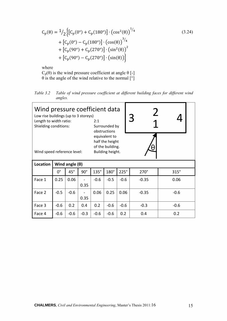
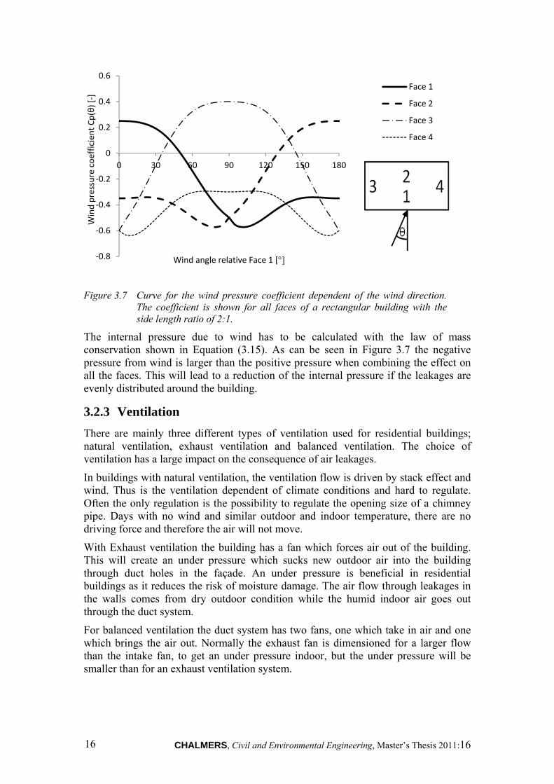
The wind pressure coefficient for a certain angle, Cp(θ), is obtained from wind tunnel experiments resulting in tables like Table 3.2. In ASHRAE (2009), corrected in ASHRAE (2010), there is a formula, shown in Equation (3.24), which makes a harmonic fit to interpolate between the angles specified in the tables. An example of the interpolation curves is shown in Figure 3.7. The curve is created from the data in Table 3.2 and this curve has been used for the numerical simulations in this work, to calculate the pressure from wind.
CHALMERS, Civil and Environmental Engineering, Master’s Thesis 2011:16 15
C θ 12 C 0° C 180° ∙ cos θ
C 0° C 180° ∙ cos θ
C 90° C 270° ∙ sin θ
C 90° C 270° ∙ sin θ
(3.24)
where Cp(θ) is the wind pressure coefficient at angle θ [-] θ is the angle of the wind relative to the normal [°]
Table 3.2 Table of wind pressure coefficient at different building faces for different wind angles.
Wind pressure coefficient dataLow rise buildings (up to 3 storeys) Length to width ratio: 2:1 Shielding conditions: Surrounded by
obstructions equivalent to half the height of the building.
Wind speed reference level: Building height.
Location Wind angle (θ)
0° 45° 90° 135° 180° 225° 270° 315°
Face 1 0.25 0.06 ‐0.35
‐0.6 ‐0.5 ‐0.6 ‐0.35 0.06
Face 2 ‐0.5 ‐0.6 ‐0.35
0.06 0.25 0.06 ‐0.35 ‐0.6
Face 3 ‐0.6 0.2 0.4 0.2 ‐0.6 ‐0.6 ‐0.3 ‐0.6
Face 4 ‐0.6 ‐0.6 ‐0.3 ‐0.6 ‐0.6 0.2 0.4 0.2
θ
1
2 3 4
CHALMERS, Civil and Environmental Engineering, Master’s Thesis 2011:16 16
Figure 3.7 Curve for the wind pressure coefficient dependent of the wind direction. The coefficient is shown for all faces of a rectangular building with the side length ratio of 2:1.
The internal pressure due to wind has to be calculated with the law of mass conservation shown in Equation (3.15). As can be seen in Figure 3.7 the negative pressure from wind is larger than the positive pressure when combining the effect on all the faces. This will lead to a reduction of the internal pressure if the leakages are evenly distributed around the building.
3.2.3 Ventilation
There are mainly three different types of ventilation used for residential buildings; natural ventilation, exhaust ventilation and balanced ventilation. The choice of ventilation has a large impact on the consequence of air leakages.
In buildings with natural ventilation, the ventilation flow is driven by stack effect and wind. Thus is the ventilation dependent of climate conditions and hard to regulate. Often the only regulation is the possibility to regulate the opening size of a chimney pipe. Days with no wind and similar outdoor and indoor temperature, there are no driving force and therefore the air will not move.
With Exhaust ventilation the building has a fan which forces air out of the building. This will create an under pressure which sucks new outdoor air into the building through duct holes in the façade. An under pressure is beneficial in residential buildings as it reduces the risk of moisture damage. The air flow through leakages in the walls comes from dry outdoor condition while the humid indoor air goes out through the duct system.
For balanced ventilation the duct system has two fans, one which take in air and one which brings the air out. Normally the exhaust fan is dimensioned for a larger flow than the intake fan, to get an under pressure indoor, but the under pressure will be smaller than for an exhaust ventilation system.
‐0.8
‐0.6
‐0.4
‐0.2
0
0.2
0.4
0.6
0 30 60 90 120 150 180
Wind pressure coefficien
t Cp(θ) [‐]
Wind angle relative Face 1 [°]
Face 1
Face 2
Face 3
Face 4
CHALMERS, Civil and Environmental Engineering, Master’s Thesis 2011:16 17
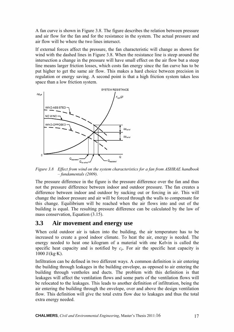
A fan curve is shown in Figure 3.8. The figure describes the relation between pressure and air flow for the fan and for the resistance in the system. The actual pressure and air flow will be where the two lines intersect.
If external forces affect the pressure, the fan characteristic will change as shown for wind with the dashed lines in Figure 3.8. When the resistance line is steep around the intersection a change in the pressure will have small effect on the air flow but a steep line means larger friction losses, which costs fan energy since the fan curve has to be put higher to get the same air flow. This makes a hard choice between precision in regulation or energy saving. A second point is that a high friction system takes less space than a low friction system.
Figure 3.8 Effect from wind on the system characteristics for a fan from ASHRAE handbook
– fundamentals (2009).
The pressure difference in the figure is the pressure difference over the fan and thus not the pressure difference between indoor and outdoor pressure. The fan creates a difference between indoor and outdoor by sucking out or forcing in air. This will change the indoor pressure and air will be forced through the walls to compensate for this change. Equilibrium will be reached when the air flows into and out of the building is equal. The resulting pressure difference can be calculated by the law of mass conservation, Equation (3.15).
3.3 Air movement and energy use When cold outdoor air is taken into the building, the air temperature has to be increased to create a good indoor climate. To heat the air, energy is needed. The energy needed to heat one kilogram of a material with one Kelvin is called the specific heat capacity and is notified by cp. For air the specific heat capacity is 1000 J/(kg·K).
Infiltration can be defined in two different ways. A common definition is air entering the building through leakages in the building envelope, as opposed to air entering the building through ventholes and ducts. The problem with this definition is that leakages will affect the ventilation flows and some parts of the ventilation flows will be relocated to the leakages. This leads to another definition of infiltration, being the air entering the building through the envelope, over and above the design ventilation flow. This definition will give the total extra flow due to leakages and thus the total extra energy needed.
CHALMERS, Civil and Environmental Engineering, Master’s Thesis 2011:16 18
Since energy use is the focus in this report, the second definition is used. It would however be more complicated if heat recycling were accounted for, since some of the design ventilation flow then might pass outside of the heat recycling system.
So from the calculated extra airflow due to leakages, i.e. the second definition, the effect needed to heat the air which flows into a building can be calculated with Equation (3.25). With the equation for effect, the energy cost from infiltration during a time period n·Δt can be calculated with Equation (3.26) where Δt is the time step over which the temperature and infiltration condition is averaged.
An averaged model to calculate the energy is shown in Equation (3.27). The averaging of the infiltration flow is a simplification. But since the ventilation and the transmission also can be described as a constant multiplied with the degree hours, DH. The simplification makes it easier to combine the effect of different energy losses.
∆ (3.25)
, ∆ ∆
(3.26)
, (3.27)
∆ ∆
(3.28)
where is the power [W] is the air flow [m3/s] is the air density [kg/m3] is the specific heat capacity [J/(kg·K)]
∆ is the temperature raise for which the energy is calculated [K] is the energy needed to heat the infiltrated air [J] is the infiltration air flow [m3/s]
∆ is the length of the time step [s] is the product of the heating hours and the temperature difference over the
year [K·h]
CHALMERS, Civil and Environmental Engineering, Master’s Thesis 2011:16 19
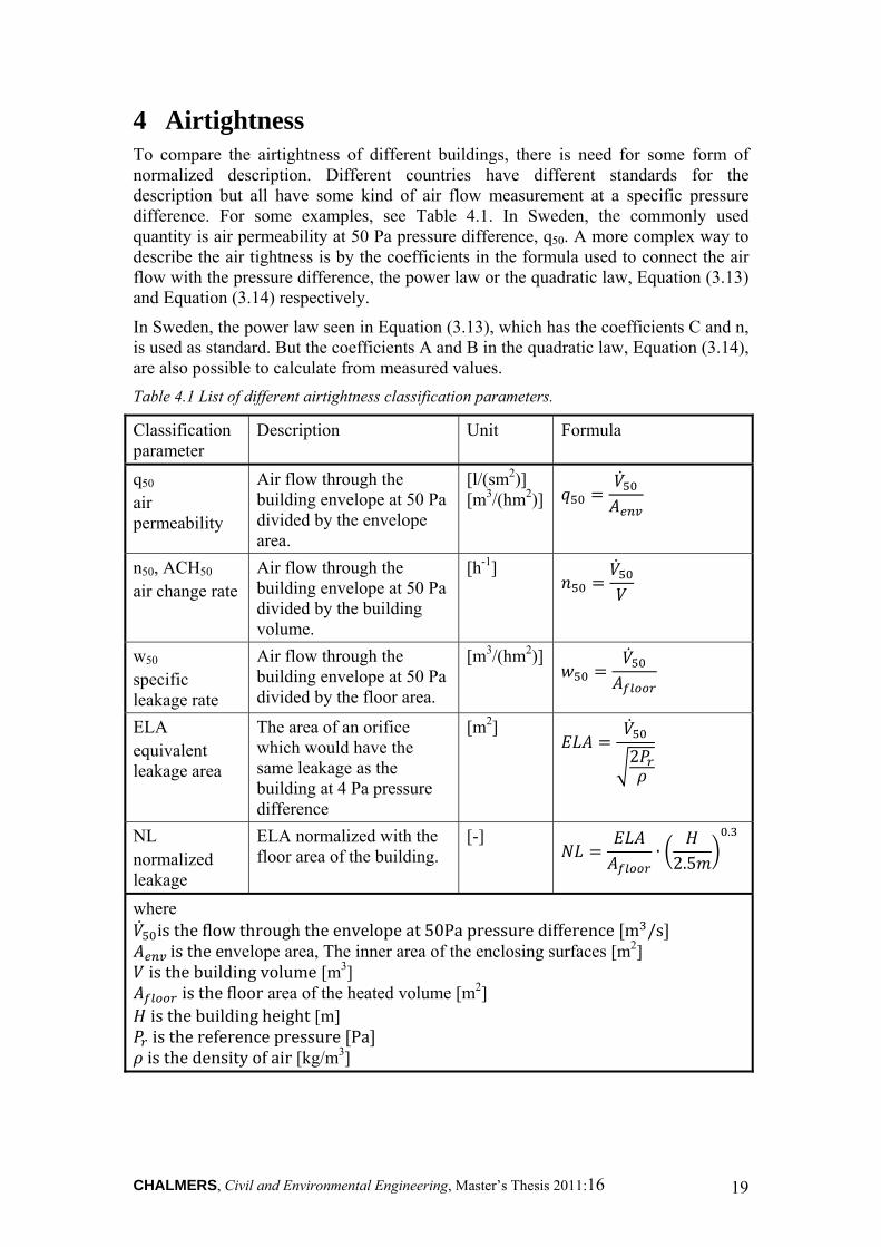
4 Airtightness To compare the airtightness of different buildings, there is need for some form of normalized description. Different countries have different standards for the description but all have some kind of air flow measurement at a specific pressure difference. For some examples, see Table 4.1. In Sweden, the commonly used quantity is air permeability at 50 Pa pressure difference, q50. A more complex way to describe the air tightness is by the coefficients in the formula used to connect the air flow with the pressure difference, the power law or the quadratic law, Equation (3.13) and Equation (3.14) respectively.
In Sweden, the power law seen in Equation (3.13), which has the coefficients C and n, is used as standard. But the coefficients A and B in the quadratic law, Equation (3.14), are also possible to calculate from measured values.
Table 4.1 List of different airtightness classification parameters.
Classification parameter
Description Unit Formula
q50 air permeability
Air flow through the building envelope at 50 Pa divided by the envelope area.
[l/(sm2)] [m3/(hm2)]
n50, ACH50
air change rate Air flow through the building envelope at 50 Pa divided by the building volume.
[h-1]
w50
specific leakage rate
Air flow through the building envelope at 50 Pa divided by the floor area.
[m3/(hm2)]
ELA equivalent leakage area
The area of an orifice which would have the same leakage as the building at 4 Pa pressure difference
[m2]
2
NL normalized leakage
ELA normalized with the floor area of the building.
[-] ∙2.5
.
where istheflowthroughtheenvelope at 50Pa pressure difference m /s istheenvelope area, The inner area of the enclosing surfaces [m2]
isthebuildingvolume [m3] isthefloor area of the heated volume [m2]
isthebuildingheight [m] isthereference pressure Pa isthedensityof air [kg/m3]
CHALMERS, Civil and Environmental Engineering, Master’s Thesis 2011:16 20
4.1 Codes for airtightness In Sweden, the regulations for the air tightness from 1994 were a maximum leakage of 0.8 l/s m2 at 50 Pa (Boverket, 1993, with changes to BFS 2005:17 BBR 11). In the changes BFS 2006:12 BBR 12, the regulation is changed to a performance based form. There the energy use is regulated and it is up to the builder to choose how to fulfill the requirements. Thus there is no direct requirement on air tightness but the energy usage due to airtightness has to be taken into consideration. The energy requirements are shown in Table 4.2, where climate zone I is for the northern counties, zone II is for the middle counties and zone III for the southern counties as specified in the table.
Table 4.2 The maximum allowed energy usage by newly built residential buildings in Sweden which are not heated by direct electricity (Boverket, 2009).
Climate zone I II III
Specific energy usage [kWh/m2year]
150 130 110
Counties in each Climate zone
I. Norrbotten, Västerbotten and Jämtland County.
II. Västernorrland, Gävleborg, Dalarna and Värmland County.
III. Västra Götaland, Jönköping, Kronoberg, Kalmar, Östergötland, Södermanland, Örebro, Västmanland, Stockholm, Uppsala, Skåne, Halland, Blekinge and Gotland County.
There are some special cases where the air tightness is specified. In BBR, there is alternative set of requirements for small houses, with a floor area of less than 100 m2 where the airtightness is specified to a leakage maximum of 0.6 l/s m2 at 50 Pa.
Disconnected from Swedish regulations there is also an airtightness demand for passive houses. Passive houses are buildings built with a focus on energy efficiency. The idea is that the internal heat production from occupants and home appliances should be enough to heat the building, most part of the year. To have a building certified as a passive house, the air tightness has to be less than 0.3 l/(s·m2) at 50 Pa pressure difference (FEBY, 2009).
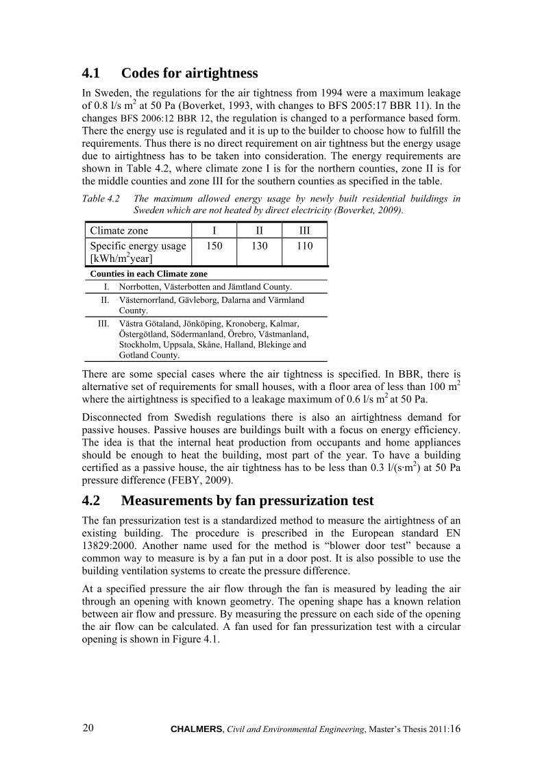
4.2 Measurements by fan pressurization test The fan pressurization test is a standardized method to measure the airtightness of an existing building. The procedure is prescribed in the European standard EN 13829:2000. Another name used for the method is “blower door test” because a common way to measure is by a fan put in a door post. It is also possible to use the building ventilation systems to create the pressure difference.
At a specified pressure the air flow through the fan is measured by leading the air through an opening with known geometry. The opening shape has a known relation between air flow and pressure. By measuring the pressure on each side of the opening the air flow can be calculated. A fan used for fan pressurization test with a circular opening is shown in Figure 4.1.
CHALMERS, Civil and Environmental Engineering, Master’s Thesis 2011:16 21
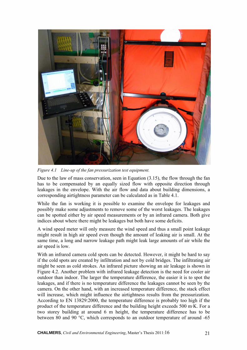
Figure 4.1 Line-up of the fan pressurization test equipment.
Due to the law of mass conservation, seen in Equation (3.15), the flow through the fan has to be compensated by an equally sized flow with opposite direction through leakages in the envelope. With the air flow and data about building dimensions, a corresponding airtightness parameter can be calculated as in Table 4.1.
While the fan is working it is possible to examine the envelope for leakages and possibly make some adjustments to remove some of the worst leakages. The leakages can be spotted either by air speed measurements or by an infrared camera. Both give indices about where there might be leakages but both have some deficits.
A wind speed meter will only measure the wind speed and thus a small point leakage might result in high air speed even though the amount of leaking air is small. At the same time, a long and narrow leakage path might leak large amounts of air while the air speed is low.
With an infrared camera cold spots can be detected. However, it might be hard to say if the cold spots are created by infiltration and not by cold bridges. The infiltrating air might be seen as cold strokes. An infrared picture showing an air leakage is shown in Figure 4.2. Another problem with infrared leakage detection is the need for cooler air outdoor than indoor. The larger the temperature difference, the easier it is to spot the leakages, and if there is no temperature difference the leakages cannot be seen by the camera. On the other hand, with an increased temperature difference, the stack effect will increase, which might influence the airtightness results from the pressurization. According to EN 13829:2000, the temperature difference is probably too high if the product of the temperature difference and the building height exceeds 500 m·K. For a two storey building at around 6 m height, the temperature difference has to be between 80 and 90 °C, which corresponds to an outdoor temperature of around -65
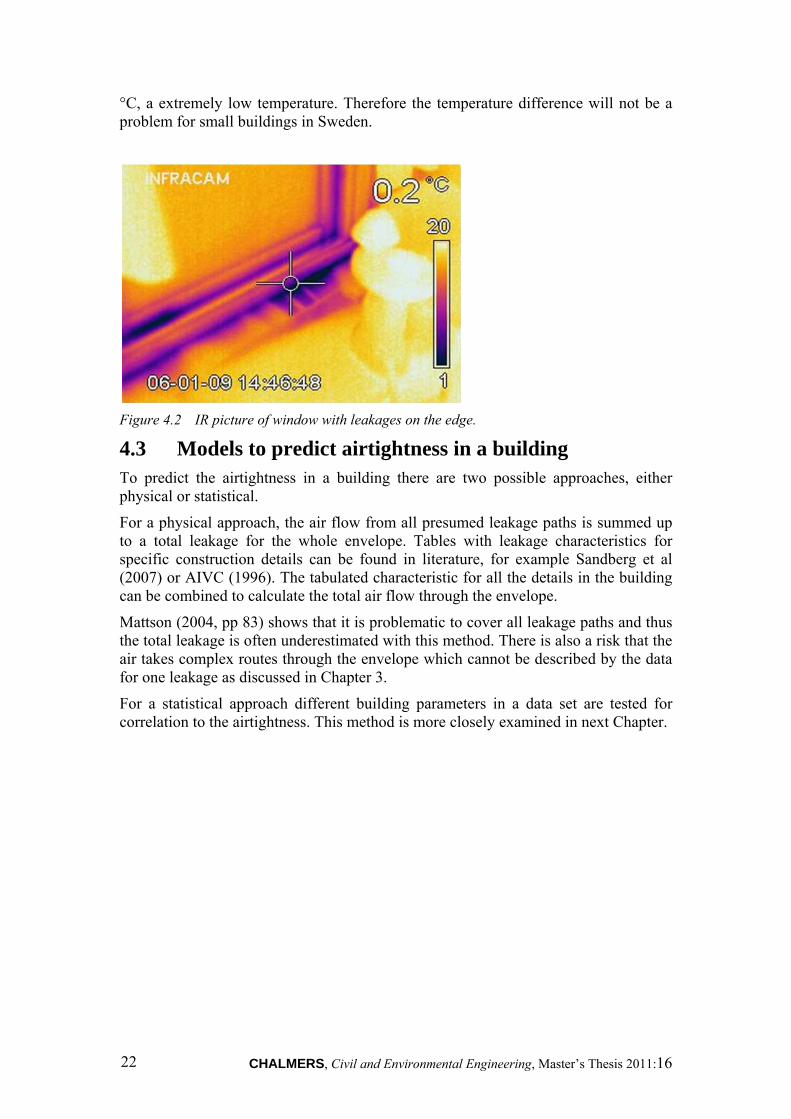
CHALMERS, Civil and Environmental Engineering, Master’s Thesis 2011:16 22
°C, a extremely low temperature. Therefore the temperature difference will not be a problem for small buildings in Sweden.
Figure 4.2 IR picture of window with leakages on the edge.
4.3 Models to predict airtightness in a building To predict the airtightness in a building there are two possible approaches, either physical or statistical.
For a physical approach, the air flow from all presumed leakage paths is summed up to a total leakage for the whole envelope. Tables with leakage characteristics for specific construction details can be found in literature, for example Sandberg et al (2007) or AIVC (1996). The tabulated characteristic for all the details in the building can be combined to calculate the total air flow through the envelope.
Mattson (2004, pp 83) shows that it is problematic to cover all leakage paths and thus the total leakage is often underestimated with this method. There is also a risk that the air takes complex routes through the envelope which cannot be described by the data for one leakage as discussed in Chapter 3.
For a statistical approach different building parameters in a data set are tested for correlation to the airtightness. This method is more closely examined in next Chapter.
CHALMERS, Civil and Environmental Engineering, Master’s Thesis 2011:16 23
5 Statistical models for airtightness prediction This chapter analyzes statistical models for airtightness prediction. The first part is a literature study about which factors that might affect the air tightness, and after that the three statistical models by McWilliams et al (2006), Montoya et al (2010) and Zou (2010) are explained.
The foreign models by McWilliams et al (2006) from USA and Montoya et al (2010) from Catalonia are both adjusted to a Swedish database with a least square method regression.
5.1 Factors influencing air tightness
As opposed to a physical model, a statistical model does not have to rely on physical characteristics of the building. It can also consider qualitative characteristics of the building process.
An important step in setting up a statistical model is therefore to find out which factors that could affect the airtightness. With a guess of influencing factors, information about these can be obtained in connection with pressurization tests and the actual correlation can be calculated.
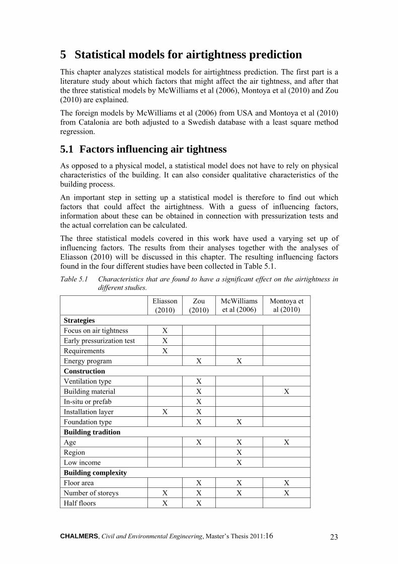
The three statistical models covered in this work have used a varying set up of influencing factors. The results from their analyses together with the analyses of Eliasson (2010) will be discussed in this chapter. The resulting influencing factors found in the four different studies have been collected in Table 5.1.
Table 5.1 Characteristics that are found to have a significant effect on the airtightness in different studies.
Eliasson (2010)
Zou (2010)
McWilliams et al (2006)
Montoya et al (2010)
Strategies Focus on air tightness X Early pressurization test X Requirements X Energy program X X
Construction Ventilation type X Building material X X In-situ or prefab X Installation layer X X Foundation type X X
Building tradition Age X X X Region X Low income X Building complexity Floor area X X X Number of storeys X X X X Half floors X X
CHALMERS, Civil and Environmental Engineering, Master’s Thesis 2011:16 24
Both Zou (2010) and McWilliams et al (2006) find that the most influencing factor for airtightness is if the building is part of a low energy use project. Even if the statistics show better airtightness for low energy houses, this factor cannot stand for itself. The actual improvement of the airtightness has to come from measures taken to ensure a low infiltration. This means that the factor is only usable to analyze already built buildings, but the underlying measures should be used for a statistical prediction of a new building.
In a similar way, Eliasson (2010) finds a correlation between the focus on airtightness and the leakage. As for energy efficient buildings, some of the effect has to come from other measures, taken because of the extra focus, but it might also be an improvement because of more accurate detail work.
Eliasson (2010) has investigated the influence of early leakage search. An early leakage search is when the building is pressurized as soon as the airtight layer is completed, before the house is finished. It means that errors in the airtight layer can be corrected while the air tight layer still is in the open. Eliasson (2010) cannot find any conclusive positive effect from this procedure and gives the reason in lack information spread. But, it might also be because a leakage search in an early stage provides knowledge about where the larger leakages are and focus gets on those leakages. Without an early leakage search the overall work has to be more detailed to guarantee that the final airtightness is good enough. This factor would need a more detailed statistical analysis where the set demands where correlated to the results.
Eliasson (2010) concludes that a set demand is fulfilled most of the time, with varying margin. This means that a set demand more or less sets an upper limit for the air leakage. What is important then is to find out which strategies that differs depending on the demands.
For construction methods, Eliassons (2010) finds that the most influencing factor is the usage of an installation layer. An installation layer is a cavity between the airtight layer and the internal wall, where the installations can be put. In this way installations do not have to penetrate the air tight layer at as many points. Eliasson (2010) finds that the mean permeability was reduced with 50 % when an installation layer was used. Also Zou (2010) concludes a statistically significant difference between the mean airtightness for a building with and without installation layer.
For wall materials, Montoya et al (2010) and Zou (2010) both find that light walls (eg. wooden stud constructions) gives a worse airtightness than heavy walls (eg. concrete constructions), even though Zou (2010) does not find the result significant. In the same way Zou (2010) does not find any significant effect of the choice of foundation type while McWilliams et al (2006) finds an increased leakage from buildings with a crawl space or unconditioned basement compared to a building with a slab on ground foundaton.
Zou (2010) has found high significance for newer houses having a lower mean permeability compared to older ones. For some time periods, the amount of buildings are too low to come to any conclusions. Above that, buildings from the 80s have not been considered since all available buildings in the study had special focus on airtightness. McWilliams et al (2006) conclude that there is a connection between age and air tightness although they find it very small, around 1% per year. They also mention the problem with separating deterioration from innovation and use of new airtightening methods. Both of which will affect the airtightness relationship to the age of the building. Montoya et al (2010) gives age a larger effect of around 8% per
CHALMERS, Civil and Environmental Engineering, Master’s Thesis 2011:16 25
year for newly built houses and above that they add an extra term for buildings of ages 9 to 64 years and another for houses older than 64 years.
Both Zou (2010) and McWilliams et al. (2006) investigate the effect of ventilation type. Zou (2010) finds no significant difference in air tightness between different ventilation types for older buildings but for newer buildings, post-2000, the houses with balanced ventilation has significantly lower average permeability. McWilliams et al (2006) comes to a similar conclusion when they combine buildings with ductworks to buildings without. The buildings with ductwork are tighter. They find this counterintuitive as the leakages usually increase with increased amount of ducts, due to leakages from the ductwork. However, many buildings with balanced ventilation are also in energy programs which might be the actual reason for the low value.
In Eliasson (2010) building complexity is analyzed. The buildings are categorized depending on the number of floors, half floors and if they are part of row houses or pair houses. Zou (2010) has made a similar comparison for number of stories and half stories. Even though Eliassons results are unclear due to the effect of row buildings both Eliasson and Zou show an increased leakage for buildings with half stories. This effect is probably derives from difficulties in making the connections when the airtight layer is folded around corners. In both McWilliams (2006) and Montanya (2009) the complexity is tested only as size parameters. Both reports show dependency on number of stories and floor area.
5.2 Prediction model for residential buildings in USA
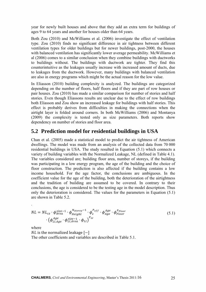
Chan et al. (2005) made a statistical model to predict the air tightness of American dwellings. The model was made from an analysis of the collected data from 70 000 residential buildings in USA. The study resulted in Equation (5.1) which connects a variety of building variables with the Normalized Leakage, NL (defined in Table 4.1). The variables considered are; building floor area, number of storeys, if the building was participating in a low energy program, the age of the building and the choice of floor construction. The prediction is also affected if the building contains a low income household. For the age factor, the conclusions are ambiguous. In the coefficient value for the age of the building, both the deterioration of the airtightness and the tradition of building are assumed to be covered. In contrary to their conclusions, the age is considered to be the testing age in the model description. Thus only the deterioration is considered. The values for the parameters in Equation (5.1) are shown in Table 5.2.
.
∙ ∙ ∙ ∙ ∙
∙ , ∙ , ∙
(5.1)
where isthenormalizedleakage
The other coefficients and variables are described in Table 5.1.
CHALMERS, Civil and Environmental Engineering, Master’s Thesis 2011:16 26
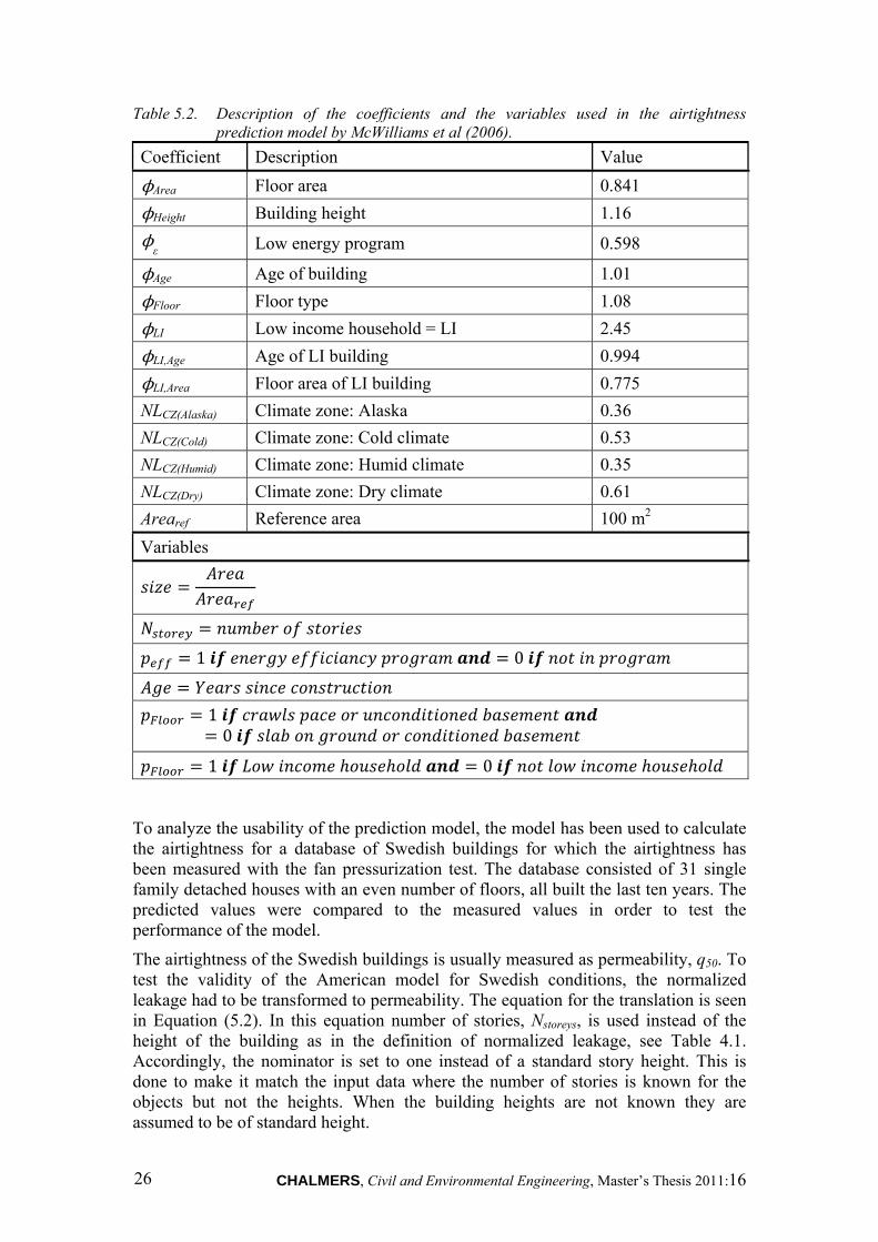
Table 5.2. Description of the coefficients and the variables used in the airtightness prediction model by McWilliams et al (2006).
Coefficient Description Value
ϕArea Floor area 0.841
ϕHeight Building height 1.16
ϕε Low energy program 0.598
ϕAge Age of building 1.01
ϕFloor Floor type 1.08
ϕLI Low income household = LI 2.45
ϕLI,Age Age of LI building 0.994
ϕLI,Area Floor area of LI building 0.775
NLCZ(Alaska) Climate zone: Alaska 0.36
NLCZ(Cold) Climate zone: Cold climate 0.53
NLCZ(Humid) Climate zone: Humid climate 0.35
NLCZ(Dry) Climate zone: Dry climate 0.61
Arearef Reference area 100 m2
Variables
1 0
1 0
1 0
To analyze the usability of the prediction model, the model has been used to calculate the airtightness for a database of Swedish buildings for which the airtightness has been measured with the fan pressurization test. The database consisted of 31 single family detached houses with an even number of floors, all built the last ten years. The predicted values were compared to the measured values in order to test the performance of the model.
The airtightness of the Swedish buildings is usually measured as permeability, q50. To test the validity of the American model for Swedish conditions, the normalized leakage had to be transformed to permeability. The equation for the translation is seen in Equation (5.2). In this equation number of stories, Nstoreys, is used instead of the height of the building as in the definition of normalized leakage, see Table 4.1. Accordingly, the nominator is set to one instead of a standard story height. This is done to make it match the input data where the number of stories is known for the objects but not the heights. When the building heights are not known they are assumed to be of standard height.
CHALMERS, Civil and Environmental Engineering, Master’s Thesis 2011:16 27
1000 ∙10001000
∙ ∙504
/ 4 . 1 .
14 ∙ ∙1 .
(5.2)
where is the permeability at 50 Pa pressure difference. [l/s·m2] is the total air flow at 50 Pa pressure difference. [m3/s]
is the area of the envelope. [m2] is the total floor area of the heated volume. [m2]
is the normalized leakage [-] is the air density [kg/m3]
is the number of storeys [-]
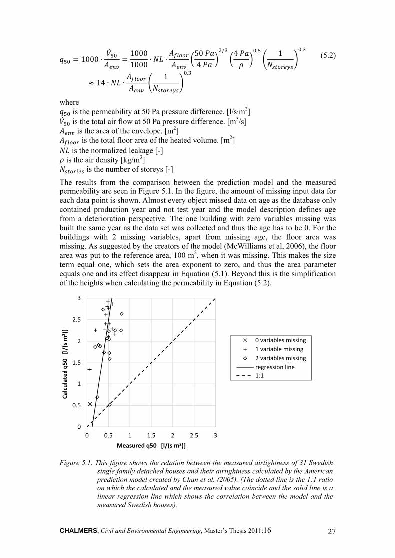
The results from the comparison between the prediction model and the measured permeability are seen in Figure 5.1. In the figure, the amount of missing input data for each data point is shown. Almost every object missed data on age as the database only contained production year and not test year and the model description defines age from a deterioration perspective. The one building with zero variables missing was built the same year as the data set was collected and thus the age has to be 0. For the buildings with 2 missing variables, apart from missing age, the floor area was missing. As suggested by the creators of the model (McWilliams et al, 2006), the floor area was put to the reference area, 100 m2, when it was missing. This makes the size term equal one, which sets the area exponent to zero, and thus the area parameter equals one and its effect disappear in Equation (5.1). Beyond this is the simplification of the heights when calculating the permeability in Equation (5.2).
Figure 5.1. This figure shows the relation between the measured airtightness of 31 Swedish
single family detached houses and their airtightness calculated by the American prediction model created by Chan et al. (2005). (The dotted line is the 1:1 ratio on which the calculated and the measured value coincide and the solid line is a linear regression line which shows the correlation between the model and the measured Swedish houses).
0
0.5
1
1.5
2
2.5
3
0 0.5 1 1.5 2 2.5 3
Calculated q50 [l/(s m
2)]
Measured q50 [l/(s m2)]
0 variables missing
1 variable missing
2 variables missing
regression line
1:1
CHALMERS, Civil and Environmental Engineering, Master’s Thesis 2011:16 28
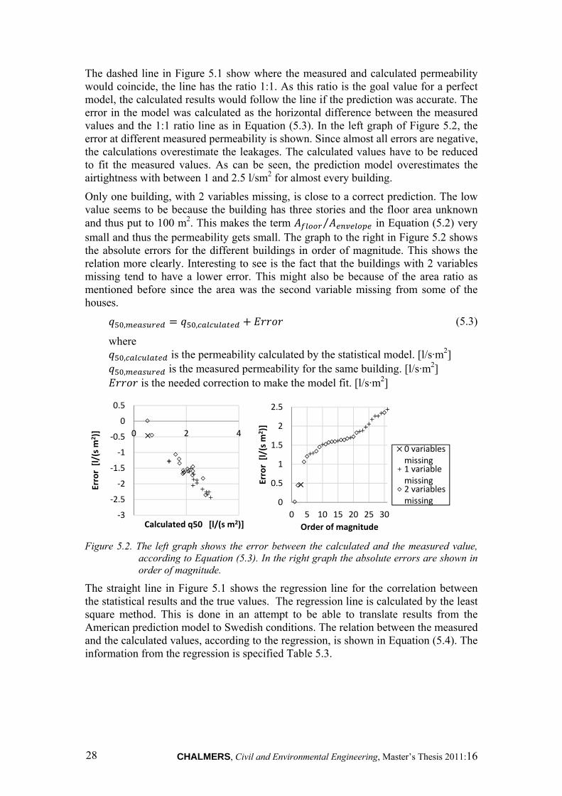
The dashed line in Figure 5.1 show where the measured and calculated permeability would coincide, the line has the ratio 1:1. As this ratio is the goal value for a perfect model, the calculated results would follow the line if the prediction was accurate. The error in the model was calculated as the horizontal difference between the measured values and the 1:1 ratio line as in Equation (5.3). In the left graph of Figure 5.2, the error at different measured permeability is shown. Since almost all errors are negative, the calculations overestimate the leakages. The calculated values have to be reduced to fit the measured values. As can be seen, the prediction model overestimates the airtightness with between 1 and 2.5 l/sm2 for almost every building.
Only one building, with 2 variables missing, is close to a correct prediction. The low value seems to be because the building has three stories and the floor area unknown and thus put to 100 m2. This makes the term ⁄ in Equation (5.2) very small and thus the permeability gets small. The graph to the right in Figure 5.2 shows the absolute errors for the different buildings in order of magnitude. This shows the relation more clearly. Interesting to see is the fact that the buildings with 2 variables missing tend to have a lower error. This might also be because of the area ratio as mentioned before since the area was the second variable missing from some of the houses.
, , (5.3)
where , is the permeability calculated by the statistical model. [l/s·m2]
, is the measured permeability for the same building. [l/s·m2] is the needed correction to make the model fit. [l/s·m2]
Figure 5.2. The left graph shows the error between the calculated and the measured value,
according to Equation (5.3). In the right graph the absolute errors are shown in order of magnitude.
The straight line in Figure 5.1 shows the regression line for the correlation between the statistical results and the true values. The regression line is calculated by the least square method. This is done in an attempt to be able to translate results from the American prediction model to Swedish conditions. The relation between the measured and the calculated values, according to the regression, is shown in Equation (5.4). The information from the regression is specified Table 5.3.
‐3
‐2.5
‐2
‐1.5
‐1
‐0.5
0
0.5
0 2 4
Error [l/(s m
2)]
Calculated q50 [l/(s m2)]
0
0.5
1
1.5
2
2.5
0 5 10 15 20 25 30
Error [l/(s m
2)]
Order of magnitude
0 variablesmissing1 variablemissing2 variablesmissing
CHALMERS, Civil and Environmental Engineering, Master’s Thesis 2011:16 29
∙ , (5.4)
where , is the permeability calculated by the statistical model. [l/s·m2] is the permeability for the building. [l/s·m2]
is the correction which would make the model fit. [l/s·m2] and are constants shown in Table 5.3.
Table 5.3 Results from the regression to find the relation between the American model and the Swedish housing stock.
Regression information
a 0.120 b 0.153 r 0.505 r2 0.256 se 0.171
The correlation between the calculated and the measured values are described by the correlation coefficient r also seen in Table 5.3. The closer to one the coefficient are, the better correlation are there. So for this regression the correlation is weak, but it shows some connection between the used factors and the measured airtightness. The squared correlation tells how much of the results that can be explained by the correlation. This means that around 75% of the resulting permeability cannot be explained by the factors used in the calculation model. This is a very low value which shows either that the influencing factors do not have a very big influence for Swedish buildings or that the regression has been made against too few buildings.
The inclination of the regression line is very steep. This means that for calculated permeabilities of between 1.5 and 3 l/(s·m2) the resulting adjusted value will be in the interval of 0.35 to 0.6 l/(s·m2) which is a very small interval compared to the standard deviation, se, of 0.171 l/(s·m2), which is more than half of the interval.
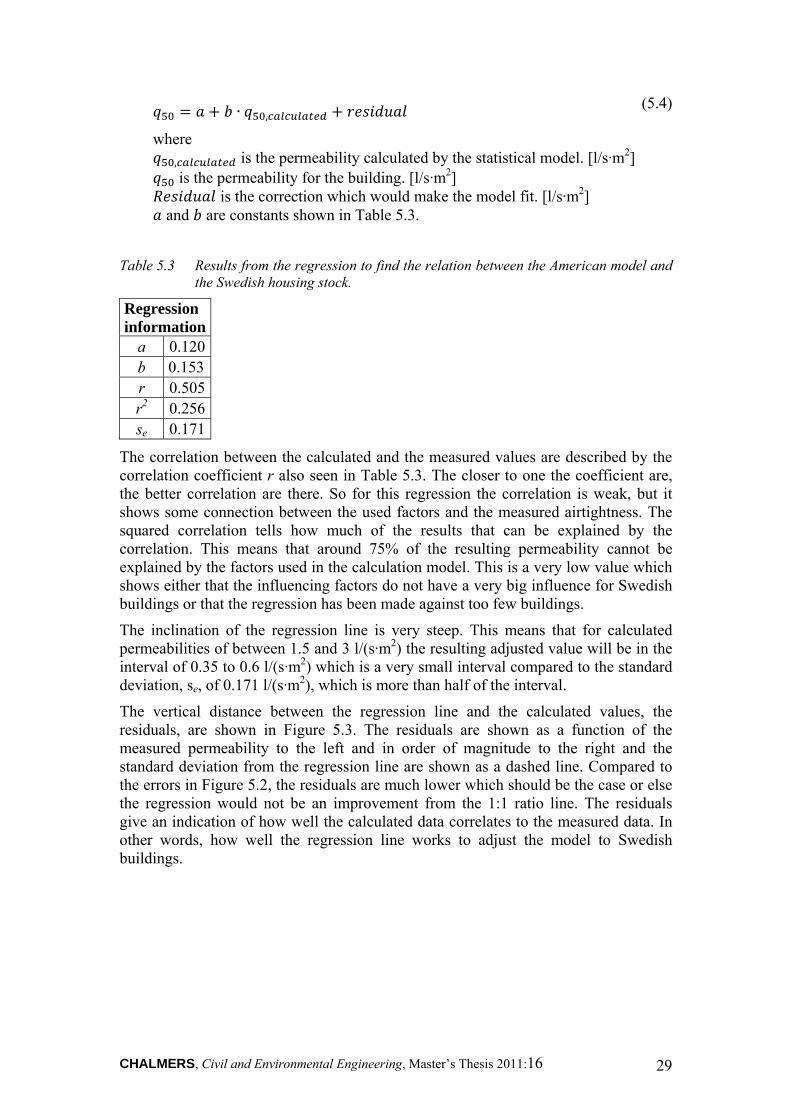
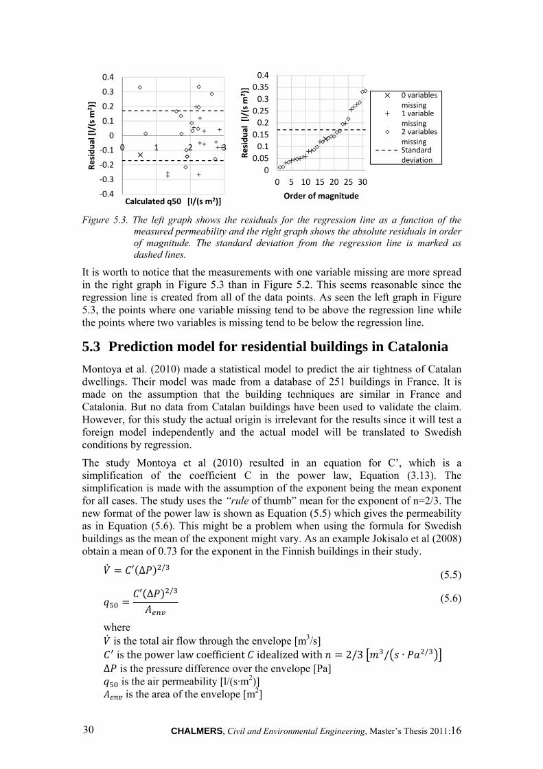
The vertical distance between the regression line and the calculated values, the residuals, are shown in Figure 5.3. The residuals are shown as a function of the measured permeability to the left and in order of magnitude to the right and the standard deviation from the regression line are shown as a dashed line. Compared to the errors in Figure 5.2, the residuals are much lower which should be the case or else the regression would not be an improvement from the 1:1 ratio line. The residuals give an indication of how well the calculated data correlates to the measured data. In other words, how well the regression line works to adjust the model to Swedish buildings.
CHALMERS, Civil and Environmental Engineering, Master’s Thesis 2011:16 30
Figure 5.3. The left graph shows the residuals for the regression line as a function of the
measured permeability and the right graph shows the absolute residuals in order of magnitude. The standard deviation from the regression line is marked as dashed lines.
It is worth to notice that the measurements with one variable missing are more spread in the right graph in Figure 5.3 than in Figure 5.2. This seems reasonable since the regression line is created from all of the data points. As seen the left graph in Figure 5.3, the points where one variable missing tend to be above the regression line while the points where two variables is missing tend to be below the regression line.
5.3 Prediction model for residential buildings in Catalonia
Montoya et al. (2010) made a statistical model to predict the air tightness of Catalan dwellings. Their model was made from a database of 251 buildings in France. It is made on the assumption that the building techniques are similar in France and Catalonia. But no data from Catalan buildings have been used to validate the claim. However, for this study the actual origin is irrelevant for the results since it will test a foreign model independently and the actual model will be translated to Swedish conditions by regression.
The study Montoya et al (2010) resulted in an equation for C’, which is a simplification of the coefficient C in the power law, Equation (3.13). The simplification is made with the assumption of the exponent being the mean exponent for all cases. The study uses the “rule of thumb” mean for the exponent of n=2/3. The new format of the power law is shown as Equation (5.5) which gives the permeability as in Equation (5.6). This might be a problem when using the formula for Swedish buildings as the mean of the exponent might vary. As an example Jokisalo et al (2008) obtain a mean of 0.73 for the exponent in the Finnish buildings in their study.
′ ∆ / (5.5)
′ ∆ /
(5.6)
where is the total air flow through the envelope [m3/s] is thepowerlawcoefficient idealizedwith 2/3 / ∙ /
∆ is the pressure difference over the envelope [Pa] is the air permeability [l/(s·m2)] is the area of the envelope [m2]
‐0.4
‐0.3
‐0.2
‐0.1
0
0.1
0.2
0.3
0.4
0 1 2 3
Residual [l/(s m
2)]
Calculated q50 [l/(s m2)]
0
0.05
0.1
0.15
0.2
0.25
0.3
0.35
0.4
0 5 10 15 20 25 30
Residual [l/(s m
2)]
Order of magnitude
0 variablesmissing1 variablemissing2 variablesmissingStandarddeviation
CHALMERS, Civil and Environmental Engineering, Master’s Thesis 2011:16 31
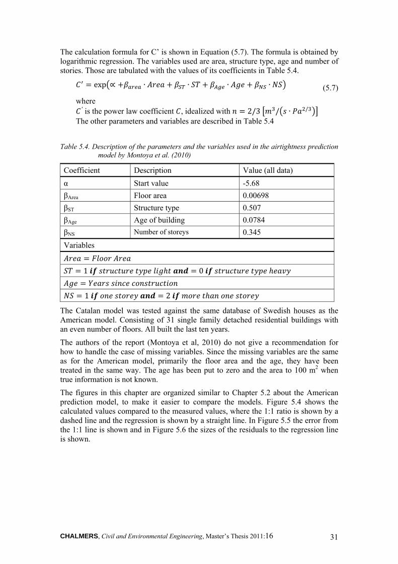
The calculation formula for C’ is shown in Equation (5.7). The formula is obtained by logarithmic regression. The variables used are area, structure type, age and number of stories. Those are tabulated with the values of its coefficients in Table 5.4.
exp ∝ ∙ ∙ ∙ ∙ (5.7)
where ′ is the power law coefficient , idealized with 2/3 / ∙ /
The other parameters and variables are described in Table 5.4
Table 5.4. Description of the parameters and the variables used in the airtightness prediction model by Montoya et al. (2010)
Coefficient Description Value (all data)
α Start value -5.68
βArea Floor area 0.00698
βST Structure type 0.507
βAge Age of building 0.0784
βNS Number of storeys 0.345
Variables
1 0
1 2
The Catalan model was tested against the same database of Swedish houses as the American model. Consisting of 31 single family detached residential buildings with an even number of floors. All built the last ten years.
The authors of the report (Montoya et al, 2010) do not give a recommendation for how to handle the case of missing variables. Since the missing variables are the same as for the American model, primarily the floor area and the age, they have been treated in the same way. The age has been put to zero and the area to 100 m2 when true information is not known.
The figures in this chapter are organized similar to Chapter 5.2 about the American prediction model, to make it easier to compare the models. Figure 5.4 shows the calculated values compared to the measured values, where the 1:1 ratio is shown by a dashed line and the regression is shown by a straight line. In Figure 5.5 the error from the 1:1 line is shown and in Figure 5.6 the sizes of the residuals to the regression line is shown.
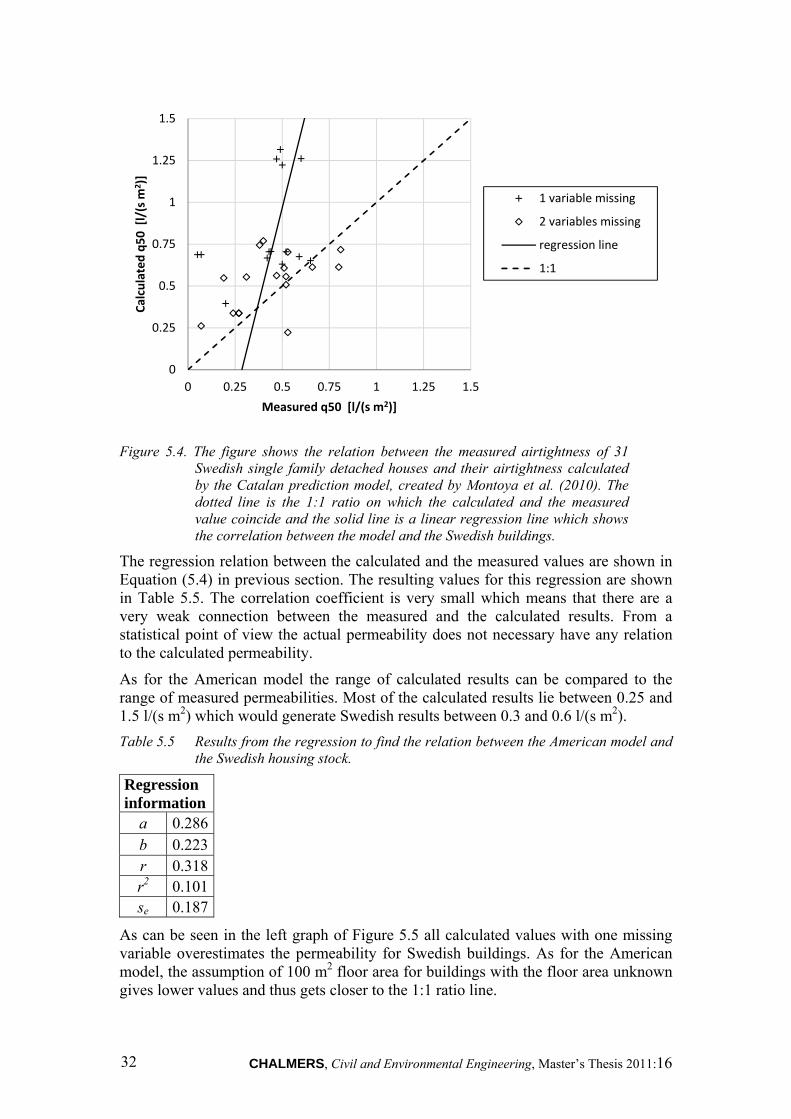
CHALMERS, Civil and Environmental Engineering, Master’s Thesis 2011:16 32
Figure 5.4. The figure shows the relation between the measured airtightness of 31
Swedish single family detached houses and their airtightness calculated by the Catalan prediction model, created by Montoya et al. (2010). The dotted line is the 1:1 ratio on which the calculated and the measured value coincide and the solid line is a linear regression line which shows the correlation between the model and the Swedish buildings.
The regression relation between the calculated and the measured values are shown in Equation (5.4) in previous section. The resulting values for this regression are shown in Table 5.5. The correlation coefficient is very small which means that there are a very weak connection between the measured and the calculated results. From a statistical point of view the actual permeability does not necessary have any relation to the calculated permeability.
As for the American model the range of calculated results can be compared to the range of measured permeabilities. Most of the calculated results lie between 0.25 and 1.5 l/(s m2) which would generate Swedish results between 0.3 and 0.6 l/(s m2).
Table 5.5 Results from the regression to find the relation between the American model and the Swedish housing stock.
Regression information
a 0.286 b 0.223 r 0.318 r2 0.101 se 0.187
As can be seen in the left graph of Figure 5.5 all calculated values with one missing variable overestimates the permeability for Swedish buildings. As for the American model, the assumption of 100 m2 floor area for buildings with the floor area unknown gives lower values and thus gets closer to the 1:1 ratio line.
0
0.25
0.5
0.75
1
1.25
1.5
0 0.25 0.5 0.75 1 1.25 1.5
Calculated q50 [l/(s m
2)]
Measured q50 [l/(s m2)]
1 variable missing
2 variables missing
regression line
1:1
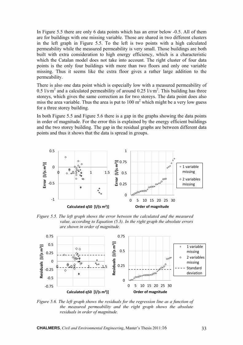
CHALMERS, Civil and Environmental Engineering, Master’s Thesis 2011:16 33
In Figure 5.5 there are only 6 data points which has an error below -0.5. All of them are for buildings with one missing variable. Those are shared in two different clusters in the left graph in Figure 5.5. To the left is two points with a high calculated permeability while the measured permeability is very small. Those buildings are both built with extra consideration to high energy efficiency, which is a characteristic which the Catalan model does not take into account. The right cluster of four data points is the only four buildings with more than two floors and only one variable missing. Thus it seems like the extra floor gives a rather large addition to the permeability.
There is also one data point which is especially low with a measured permeability of 0.5 l/s·m2 and a calculated permeability of around 0.25 l/s·m2. This building has three storeys, which gives the same correction as for two storeys. The data point does also miss the area variable. Thus the area is put to 100 m2 which might be a very low guess for a three storey building.
In both Figure 5.5 and Figure 5.6 there is a gap in the graphs showing the data points in order of magnitude. For the error this is explained by the energy efficient buildings and the two storey building. The gap in the residual graphs are between different data points and thus it shows that the data is spread in groups.
Figure 5.5. The left graph shows the error between the calculated and the measured
value, according to Equation (5.3). In the right graph the absolute errors are shown in order of magnitude.
Figure 5.6. The left graph shows the residuals for the regression line as a function of
the measured permeability and the right graph shows the absolute residuals in order of magnitude.
‐1
‐0.5
0
0.5
0 0.5 1 1.5
Error[l/(s m
2)]
Calculated q50 [l/(s m2)]
0
0.25
0.5
0.75
1
0 5 10 15 20 25 30
Error[l/(s m
2)]
Order of magnitude
1 variablemissing
2 variablesmissing
‐0.75
‐0.5
‐0.25
0
0.25
0.5
0.75
0 0.5 1 1.5
Residuals[l/(s m
2)]
Calculated q50 [l/(s m2)]
0
0.25
0.5
0.75
0 5 10 15 20 25 30
Residuals[l/(s m
2)]
Order of magnitude
1 variablemissing
2 variablesmissing
Standarddeviation
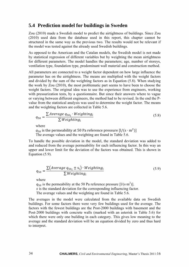
CHALMERS, Civil and Environmental Engineering, Master’s Thesis 2011:16 34
5.4 Prediction model for buildings in Sweden
Zou (2010) made a Swedish model to predict the airtightness of buildings. Since Zou (2010) used data from the database used in this report, this chapter cannot be structured in the same way as the previous two. The results would not be relevant if the model was tested against the already used Swedish buildings.
As opposed to the American and the Catalan models, the Swedish model is not made by statistical regression of different variables but by weighting the mean airtightness for different parameters. The model handles the parameters; age, number of storeys, ventilation type, foundation type, predominant wall material and construction method.
All parameters are connected to a weight factor dependent on how large influence the parameter has on the airtightness. The means are multiplied with the weight factors and divided by the sum of the weighting factors as in Equation (5.8). When studying the work by Zou (2010), the most problematic part seems to have been to choose the weight factors. The original idea was to use the experience from engineers, working with pressurization tests, by a questionnaire. But since their answers where to vague or varying between different engineers, the method had to be revised. In the end the P-value from the statistical analysis was used to determine the weight factor. The means and the weighting factors are collected in Table 5.6.
∑ ∙∑
(5.8)
where isthepermeabilityat50 Pa reference pressure l/ s ∙ m
The average values and the weighting are found in Table 5.6.
To handle the possible deviation in the model, the standard deviation was added to and reduced from the average permeability for each influencing factor. In this way an upper and lower limit for the deviation of the factors was obtained. This is shown in Equation (5.9).
∑ s ∙∑
(5.9)
where is the permeability at the 50 Pa reference pressure [l/(s·m2)].
is the standard deviation for the corresponding influencing factor. The average values and the weighting are found in Table 5.6.
The averages in the model were calculated from the available data on Swedish buildings. For some factors there were very few buildings used for the average. The factors with the fewest buildings are the Post-2000 buildings with basement and the Post-2000 buildings with concrete walls (marked with an asterisk in Table 5.6) for which there were only one building in each category. This gives low meaning to the average and the standard deviation will be an equation divided by zero and thus hard to interpret.
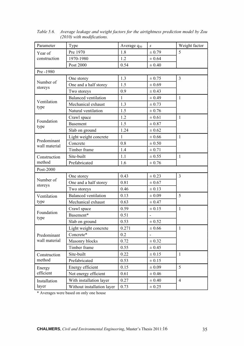
CHALMERS, Civil and Environmental Engineering, Master’s Thesis 2011:16 35
Table 5.6. Average leakage and weight factors for the airtightness prediction model by Zou (2010) with modifications.
Parameter Type Average q50 s Weight factor
Year of construction
Pre 1970 1.8 ± 0.79 5
1970-1980 1.2 ± 0.64
Post 2000 0.54 ± 0.40
Pre -1980
Number of storeys
One storey 1.3 ± 0.75 3
One and a half storey 1.5 ± 0.69
Two storeys 0.9 ± 0.43
Ventilation type
Balanced ventilation 1 ± 0.49 1
Mechanical exhaust 1.3 ± 0.73
Natural ventilation 1.5 ± 0.76
Foundation type
Crawl space 1.2 ± 0.61 1
Basement 1.5 ± 0.87
Slab on ground 1.24 ± 0.62
Predominant wall material
Light weight concrete 1 ± 0.66 1
Concrete 0.8 ± 0.50
Timber frame 1.4 ± 0.71
Construction method
Site-built 1.1 ± 0.55 1
Prefabricated 1.6 ± 0.76
Post-2000
Number of storeys
One storey 0.43 ± 0.23 3
One and a half storey 0.81 ± 0.67
Two storeys 0.46 ± 0.13
Ventilation type
Balanced ventilation 0.13 ± 0.09 5
Mechanical exhaust 0.63 ± 0.47
Foundation type
Crawl space 0.59 ± 0.15 1
Basement* 0.51 -
Slab on ground 0.53 ± 0.52
Predominant wall material
Light weight concrete 0.271 ± 0.66 1
Concrete* 0.2 -
Masonry blocks 0.72 ± 0.32
Timber frame 0.55 ± 0.45
Construction method
Site-built 0.22 ± 0.15 1
Prefabricated 0.53 ± 0.15
Energy efficient
Energy efficient 0.15 ± 0.09 5
Not energy efficient 0.61 ± 0.46
Installation layer
With installation layer 0.27 ± 0.40 4
Without installation layer 0.73 ± 0.25 * Averages were based on only one house
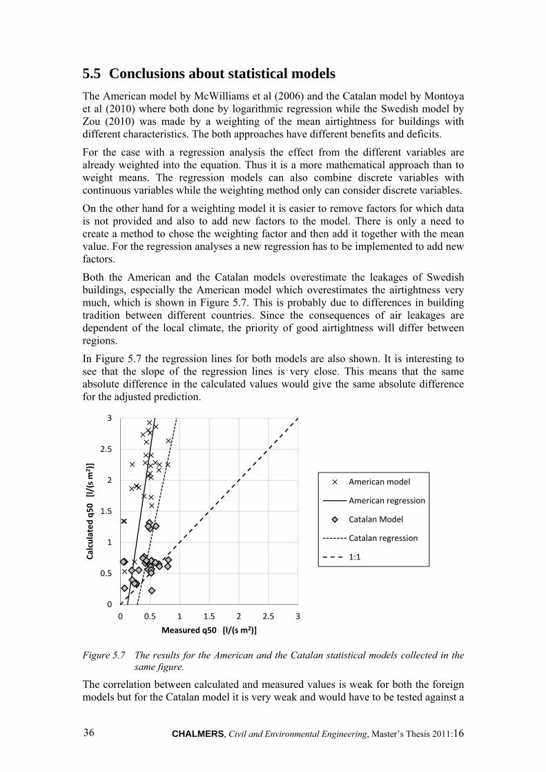
CHALMERS, Civil and Environmental Engineering, Master’s Thesis 2011:16 36
5.5 Conclusions about statistical models
The American model by McWilliams et al (2006) and the Catalan model by Montoya et al (2010) where both done by logarithmic regression while the Swedish model by Zou (2010) was made by a weighting of the mean airtightness for buildings with different characteristics. The both approaches have different benefits and deficits.
For the case with a regression analysis the effect from the different variables are already weighted into the equation. Thus it is a more mathematical approach than to weight means. The regression models can also combine discrete variables with continuous variables while the weighting method only can consider discrete variables.
On the other hand for a weighting model it is easier to remove factors for which data is not provided and also to add new factors to the model. There is only a need to create a method to chose the weighting factor and then add it together with the mean value. For the regression analyses a new regression has to be implemented to add new factors.
Both the American and the Catalan models overestimate the leakages of Swedish buildings, especially the American model which overestimates the airtightness very much, which is shown in Figure 5.7. This is probably due to differences in building tradition between different countries. Since the consequences of air leakages are dependent of the local climate, the priority of good airtightness will differ between regions.
In Figure 5.7 the regression lines for both models are also shown. It is interesting to see that the slope of the regression lines is very close. This means that the same absolute difference in the calculated values would give the same absolute difference for the adjusted prediction.
Figure 5.7 The results for the American and the Catalan statistical models collected in the
same figure.
The correlation between calculated and measured values is weak for both the foreign models but for the Catalan model it is very weak and would have to be tested against a
0
0.5
1
1.5
2
2.5
3
0 0.5 1 1.5 2 2.5 3
Calculated q50 [l/(s m
2)]
Measured q50 [l/(s m2)]
American model
American regression
Catalan Model
Catalan regression
1:1
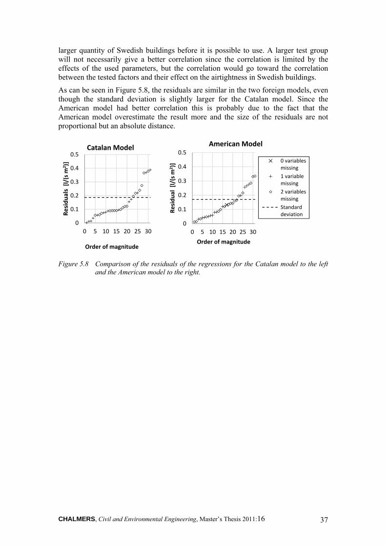
CHALMERS, Civil and Environmental Engineering, Master’s Thesis 2011:16 37
larger quantity of Swedish buildings before it is possible to use. A larger test group will not necessarily give a better correlation since the correlation is limited by the effects of the used parameters, but the correlation would go toward the correlation between the tested factors and their effect on the airtightness in Swedish buildings.
As can be seen in Figure 5.8, the residuals are similar in the two foreign models, even though the standard deviation is slightly larger for the Catalan model. Since the American model had better correlation this is probably due to the fact that the American model overestimate the result more and the size of the residuals are not proportional but an absolute distance.
Figure 5.8 Comparison of the residuals of the regressions for the Catalan model to the left
and the American model to the right.
0
0.1
0.2
0.3
0.4
0.5
0 5 10 15 20 25 30
Residuals[l/(s m
2)]
Order of magnitude
Catalan Model
0
0.1
0.2
0.3
0.4
0.5
0 5 10 15 20 25 30
Residual [l/(s m
2)]
Order of magnitude
American Model
0 variablesmissing
1 variablemissing
2 variablesmissing
Standarddeviation
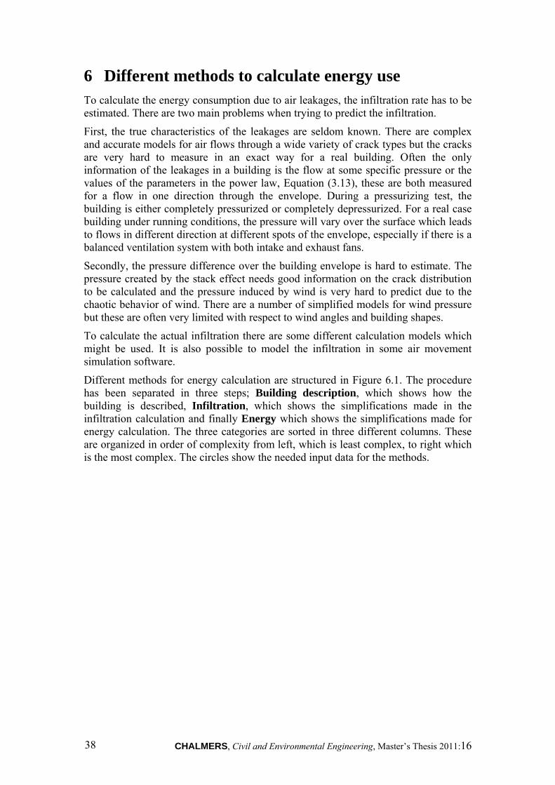
CHALMERS, Civil and Environmental Engineering, Master’s Thesis 2011:16 38
6 Different methods to calculate energy use To calculate the energy consumption due to air leakages, the infiltration rate has to be estimated. There are two main problems when trying to predict the infiltration.
First, the true characteristics of the leakages are seldom known. There are complex and accurate models for air flows through a wide variety of crack types but the cracks are very hard to measure in an exact way for a real building. Often the only information of the leakages in a building is the flow at some specific pressure or the values of the parameters in the power law, Equation (3.13), these are both measured for a flow in one direction through the envelope. During a pressurizing test, the building is either completely pressurized or completely depressurized. For a real case building under running conditions, the pressure will vary over the surface which leads to flows in different direction at different spots of the envelope, especially if there is a balanced ventilation system with both intake and exhaust fans.
Secondly, the pressure difference over the building envelope is hard to estimate. The pressure created by the stack effect needs good information on the crack distribution to be calculated and the pressure induced by wind is very hard to predict due to the chaotic behavior of wind. There are a number of simplified models for wind pressure but these are often very limited with respect to wind angles and building shapes.
To calculate the actual infiltration there are some different calculation models which might be used. It is also possible to model the infiltration in some air movement simulation software.
Different methods for energy calculation are structured in Figure 6.1. The procedure has been separated in three steps; Building description, which shows how the building is described, Infiltration, which shows the simplifications made in the infiltration calculation and finally Energy which shows the simplifications made for energy calculation. The three categories are sorted in three different columns. These are organized in order of complexity from left, which is least complex, to right which is the most complex. The circles show the needed input data for the methods.
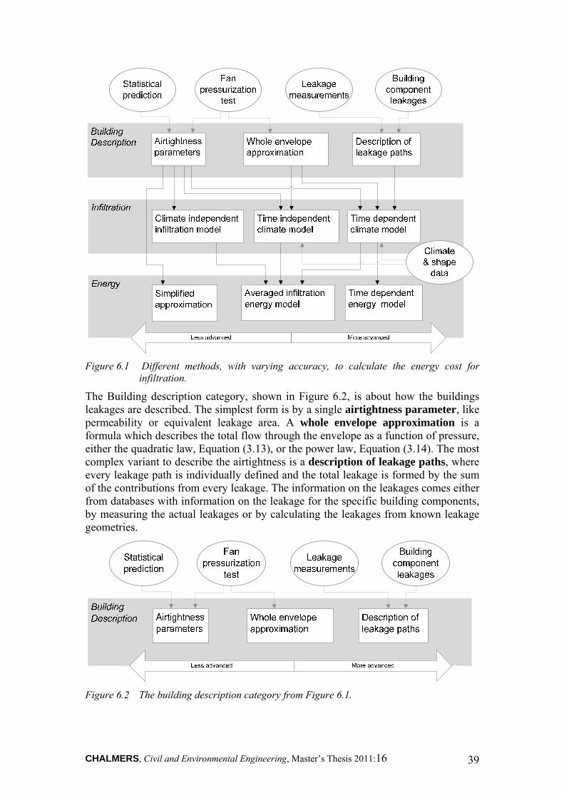
CHALMERS, Civil and Environmental Engineering, Master’s Thesis 2011:16 39
Figure 6.1 Different methods, with varying accuracy, to calculate the energy cost for infiltration.
The Building description category, shown in Figure 6.2, is about how the buildings leakages are described. The simplest form is by a single airtightness parameter, like permeability or equivalent leakage area. A whole envelope approximation is a formula which describes the total flow through the envelope as a function of pressure, either the quadratic law, Equation (3.13), or the power law, Equation (3.14). The most complex variant to describe the airtightness is a description of leakage paths, where every leakage path is individually defined and the total leakage is formed by the sum of the contributions from every leakage. The information on the leakages comes either from databases with information on the leakage for the specific building components, by measuring the actual leakages or by calculating the leakages from known leakage geometries.
Figure 6.2 The building description category from Figure 6.1.
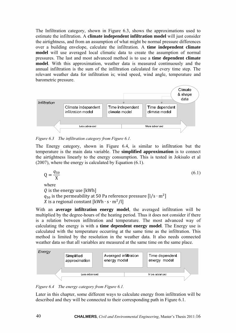
CHALMERS, Civil and Environmental Engineering, Master’s Thesis 2011:16 40
The Infiltration category, shown in Figure 6.3, shows the approximations used to estimate the infiltration. A climate independent infiltration model will just consider the airtightness, and from an assumption of what might be normal pressure differences over a building envelope, calculate the infiltration. A time independent climate model will use averaged local climatic data to create the assumption of normal pressures. The last and most advanced method is to use a time dependent climate model. With this approximation, weather data is measured continuously and the annual infiltration is the sum of the infiltration calculated for every time step. The relevant weather data for infiltration is; wind speed, wind angle, temperature and barometric pressure.
Figure 6.3 The infiltration category from Figure 6.1.
The Energy category, shown in Figure 6.4, is similar to infiltration but the temperature is the main data variable. The simplified approximation is to connect the airtightness linearly to the energy consumption. This is tested in Jokisalo et al (2007), where the energy is calculated by Equation (6.1).
QX (6.1)
where istheenergyuse kWh isthepermeabilityat50 Pa reference pressure l s ∙ m⁄
isaregional constant kWh ∙ s ∙ m /l
With an average infiltration energy model, the averaged infiltration will be multiplied by the degree-hours of the heating period. Thus it does not consider if there is a relation between infiltration and temperature. The most advanced way of calculating the energy is with a time dependent energy model. The Energy use is calculated with the temperature occurring at the same time as the infiltration. This method is limited by the resolution in the weather data. It also needs connected weather data so that all variables are measured at the same time on the same place.
Figure 6.4 The energy category from Figure 6.1.
Later in this chapter, some different ways to calculate energy from infiltration will be described and they will be connected to their corresponding path in Figure 6.1.
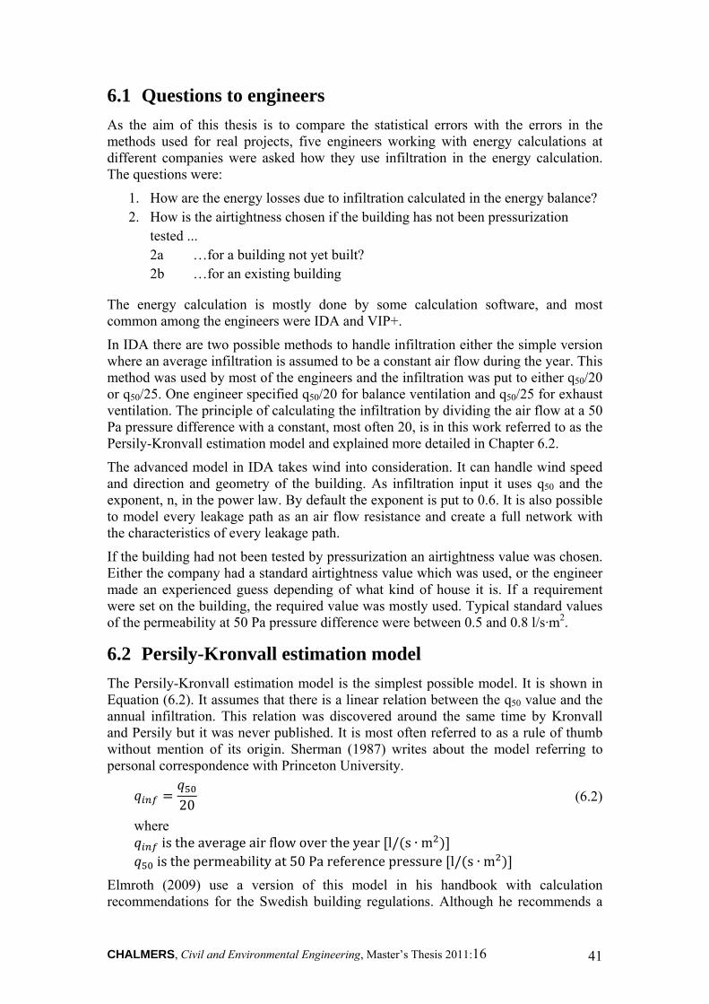
CHALMERS, Civil and Environmental Engineering, Master’s Thesis 2011:16 41
6.1 Questions to engineers
As the aim of this thesis is to compare the statistical errors with the errors in the methods used for real projects, five engineers working with energy calculations at different companies were asked how they use infiltration in the energy calculation. The questions were:
1. How are the energy losses due to infiltration calculated in the energy balance? 2. How is the airtightness chosen if the building has not been pressurization
tested ... 2a …for a building not yet built? 2b …for an existing building
The energy calculation is mostly done by some calculation software, and most common among the engineers were IDA and VIP+.
In IDA there are two possible methods to handle infiltration either the simple version where an average infiltration is assumed to be a constant air flow during the year. This method was used by most of the engineers and the infiltration was put to either q50/20 or q50/25. One engineer specified q50/20 for balance ventilation and q50/25 for exhaust ventilation. The principle of calculating the infiltration by dividing the air flow at a 50 Pa pressure difference with a constant, most often 20, is in this work referred to as the Persily-Kronvall estimation model and explained more detailed in Chapter 6.2.
The advanced model in IDA takes wind into consideration. It can handle wind speed and direction and geometry of the building. As infiltration input it uses q50 and the exponent, n, in the power law. By default the exponent is put to 0.6. It is also possible to model every leakage path as an air flow resistance and create a full network with the characteristics of every leakage path.
If the building had not been tested by pressurization an airtightness value was chosen. Either the company had a standard airtightness value which was used, or the engineer made an experienced guess depending of what kind of house it is. If a requirement were set on the building, the required value was mostly used. Typical standard values of the permeability at 50 Pa pressure difference were between 0.5 and 0.8 l/s·m2.
6.2 Persily-Kronvall estimation model
The Persily-Kronvall estimation model is the simplest possible model. It is shown in Equation (6.2). It assumes that there is a linear relation between the q50 value and the annual infiltration. This relation was discovered around the same time by Kronvall and Persily but it was never published. It is most often referred to as a rule of thumb without mention of its origin. Sherman (1987) writes about the model referring to personal correspondence with Princeton University.
20
(6.2)
where istheaverageairflow over the year l/ s ∙ m
isthepermeabilityat50 Pa reference pressure l/ s ∙ m
Elmroth (2009) use a version of this model in his handbook with calculation recommendations for the Swedish building regulations. Although he recommends a

CHALMERS, Civil and Environmental Engineering, Master’s Thesis 2011:16 42
denominator of 40 for exhaust ventilation and the regular denominator of 20 if the ventilation is balanced. As mentioned in Chapter 6.1, some of the engineers used 25 as denominator which is also used, in the form of 4% of the 50 Pa pressure difference flow, in Petersson (2007, pp.133) .
In Figure 6.5 the path in Figure 6.1 for the Persily-Kronvall estimation model is shown. The model uses the permeability at 50 Pa pressure difference, which is linearly adjusted to normal conditions by a climate independent constant. To calculate the energy an average temperature can be used since the model does not generate any transient infiltration rates.
Figure 6.5 The path in Figure 6.1 for energy calculation with Persily-Kronvall estimation
model.
6.3 LBL Infiltration Model The LBL Infiltration Model was developed at Lawrence Berkley Laboratories in the early eighties. The total flow through the envelope is calculated by superposition of the contributions from wind and stack, shown in Equation (6.3).
To describe the building the model uses the equivalent leakage area which can be obtained from a fan pressurization test. The rest of the flow terms are separated into a constant and a variable part, see Equation (6.4). For the flow from wind, the variable part is the wind speed and the constant part contains information about sheltering and terrain, see Equation (6.5). For flow from stack the variable part is the temperature difference between indoor and outdoor and the constant contains information on leakage distribution and building height, see Equation (6.6) (Sherman, 1998).
The equation follows the climate data time step and for each step the infiltration is calculated from the actual wind speed and temperature. The temperature can be used again to calculate the energy needed to heat the air.
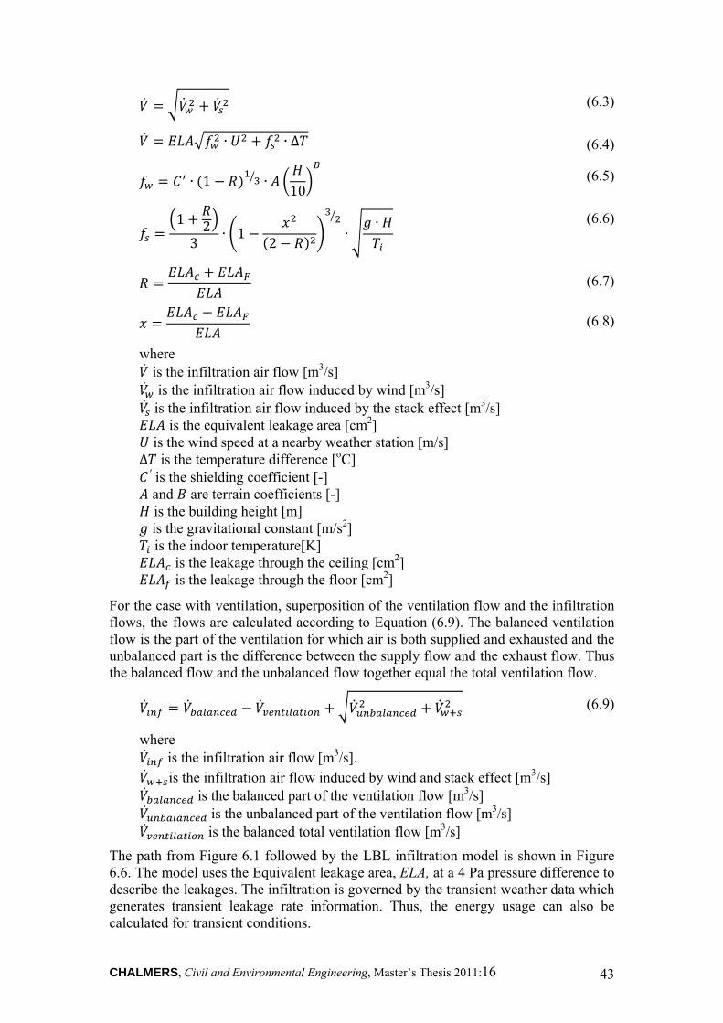
CHALMERS, Civil and Environmental Engineering, Master’s Thesis 2011:16 43
(6.3)
∙ ∙ ∆ (6.4)
∙ 1 ∙
10 (6.5)
1 23
∙ 12
∙∙
(6.6)
(6.7)
(6.8)
where
is the infiltration air flow [m3/s] is the infiltration air flow induced by wind [m3/s] is the infiltration air flow induced by the stack effect [m3/s]
is the equivalent leakage area [cm2] is the wind speed at a nearby weather station [m/s]
∆ is the temperature difference [oC] ′ is the shielding coefficient [-] and are terrain coefficients [-] is the building height [m] is the gravitational constant [m/s2] is the indoor temperature[K]
is the leakage through the ceiling [cm2] is the leakage through the floor [cm2]
For the case with ventilation, superposition of the ventilation flow and the infiltration flows, the flows are calculated according to Equation (6.9). The balanced ventilation flow is the part of the ventilation for which air is both supplied and exhausted and the unbalanced part is the difference between the supply flow and the exhaust flow. Thus the balanced flow and the unbalanced flow together equal the total ventilation flow.
(6.9)
where is the infiltration air flow [m3/s]. is the infiltration air flow induced by wind and stack effect [m3/s]
is the balanced part of the ventilation flow [m3/s] is the unbalanced part of the ventilation flow [m3/s] is the balanced total ventilation flow [m3/s]
The path from Figure 6.1 followed by the LBL infiltration model is shown in Figure 6.6. The model uses the Equivalent leakage area, ELA, at a 4 Pa pressure difference to describe the leakages. The infiltration is governed by the transient weather data which generates transient leakage rate information. Thus, the energy usage can also be calculated for transient conditions.
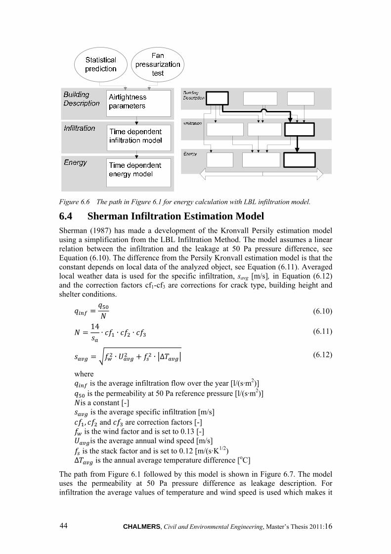
CHALMERS, Civil and Environmental Engineering, Master’s Thesis 2011:16 44
Figure 6.6 The path in Figure 6.1 for energy calculation with LBL infiltration model.
6.4 Sherman Infiltration Estimation Model Sherman (1987) has made a development of the Kronvall Persily estimation model using a simplification from the LBL Infiltration Method. The model assumes a linear relation between the infiltration and the leakage at 50 Pa pressure difference, see Equation (6.10). The difference from the Persily Kronvall estimation model is that the constant depends on local data of the analyzed object, see Equation (6.11). Averaged local weather data is used for the specific infiltration, savg [m/s], in Equation (6.12) and the correction factors cf1-cf3 are corrections for crack type, building height and shelter conditions.
(6.10)
14∙ ∙ ∙ (6.11)
∙ ∙ ∆ (6.12)
where is the average infiltration flow over the year [l/(s·m2)]
is the permeability at 50 Pa reference pressure [l/(s·m2)] is a constant [-]
is the average specific infiltration [m/s] , and are correction factors [-]
is the wind factor and is set to 0.13 [-] is the average annual wind speed [m/s]
is the stack factor and is set to 0.12 [m/(s·K1/2) ∆ is the annual average temperature difference [oC]
The path from Figure 6.1 followed by this model is shown in Figure 6.7. The model uses the permeability at 50 Pa pressure difference as leakage description. For infiltration the average values of temperature and wind speed is used which makes it
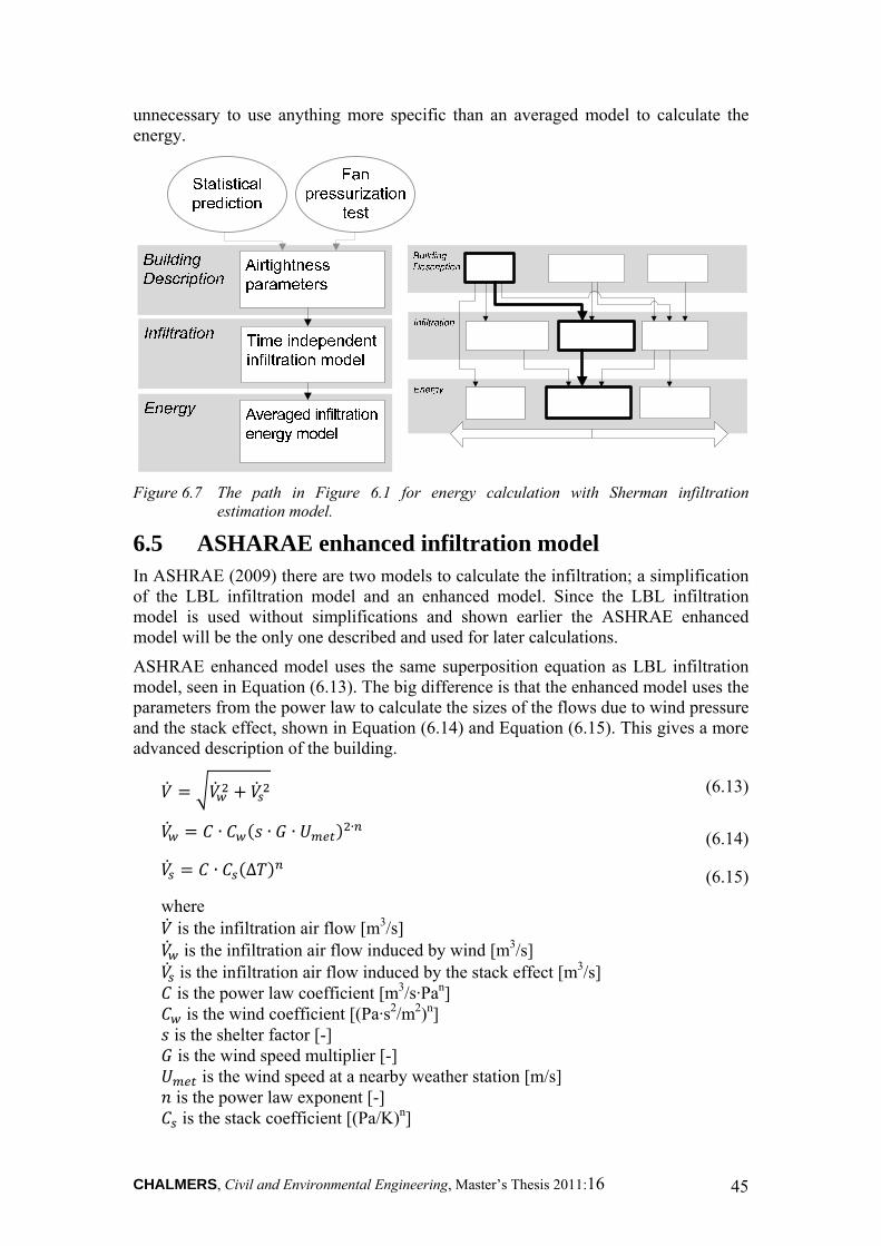
CHALMERS, Civil and Environmental Engineering, Master’s Thesis 2011:16 45
unnecessary to use anything more specific than an averaged model to calculate the energy.
Figure 6.7 The path in Figure 6.1 for energy calculation with Sherman infiltration
estimation model.
6.5 ASHARAE enhanced infiltration model In ASHRAE (2009) there are two models to calculate the infiltration; a simplification of the LBL infiltration model and an enhanced model. Since the LBL infiltration model is used without simplifications and shown earlier the ASHRAE enhanced model will be the only one described and used for later calculations.
ASHRAE enhanced model uses the same superposition equation as LBL infiltration model, seen in Equation (6.13). The big difference is that the enhanced model uses the parameters from the power law to calculate the sizes of the flows due to wind pressure and the stack effect, shown in Equation (6.14) and Equation (6.15). This gives a more advanced description of the building.
(6.13)
∙ ∙ ∙ ∙ (6.14)
∙ ∆ (6.15)
where is the infiltration air flow [m3/s] is the infiltration air flow induced by wind [m3/s] is the infiltration air flow induced by the stack effect [m3/s] is the power law coefficient [m3/s·Pan]
is the wind coefficient [(Pa·s2/m2)n] is the shelter factor [-] is the wind speed multiplier [-]
is the wind speed at a nearby weather station [m/s] is the power law exponent [-] is the stack coefficient [(Pa/K)n]
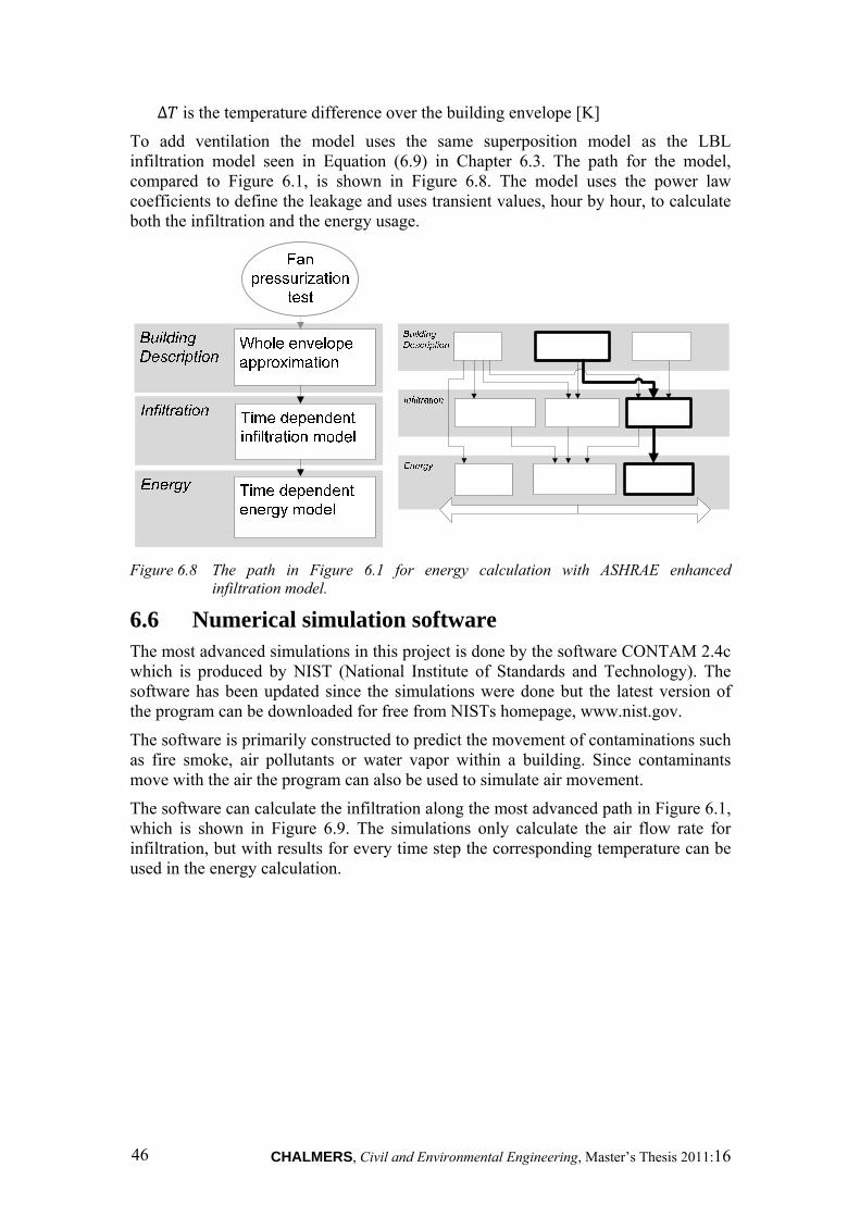
CHALMERS, Civil and Environmental Engineering, Master’s Thesis 2011:16 46
∆ is the temperature difference over the building envelope [K]
To add ventilation the model uses the same superposition model as the LBL infiltration model seen in Equation (6.9) in Chapter 6.3. The path for the model, compared to Figure 6.1, is shown in Figure 6.8. The model uses the power law coefficients to define the leakage and uses transient values, hour by hour, to calculate both the infiltration and the energy usage.
Figure 6.8 The path in Figure 6.1 for energy calculation with ASHRAE enhanced
infiltration model.
6.6 Numerical simulation software The most advanced simulations in this project is done by the software CONTAM 2.4c which is produced by NIST (National Institute of Standards and Technology). The software has been updated since the simulations were done but the latest version of the program can be downloaded for free from NISTs homepage, www.nist.gov.
The software is primarily constructed to predict the movement of contaminations such as fire smoke, air pollutants or water vapor within a building. Since contaminants move with the air the program can also be used to simulate air movement.
The software can calculate the infiltration along the most advanced path in Figure 6.1, which is shown in Figure 6.9. The simulations only calculate the air flow rate for infiltration, but with results for every time step the corresponding temperature can be used in the energy calculation.

CHALMERS, Civil and Environmental Engineering, Master’s Thesis 2011:16 47
Figure 6.9 The path in Figure 6.1 for energy calculation with the numerical simulation
software.
The set-up of a model can be done in 4 steps:
1. Define the zones of the building. 2. Define the air flow paths between the zones. 3. Define the weather conditions for the ambient zone. 4. Define the simulation method, and which results to extract.
The different steps will be described in the following sub chapters.
6.6.1 Define the zones of the building
The program can handle multiple zones but within each zone the air is considered well mixed. In other words, the condition of the air in each zone is the same, independent of where in the zone you are. The only exception is the pressure due to the stack effect which varies over the vertical dimension.
Thus, an idealization of the simulated building can be created by defining the limits of the zones of the building. In the same time the limits to the ambient zone, with outdoor air conditions, are defined. The only information that needs to be defined for each zone is its volume and a constant temperature.
Figure 6.10 To the left is a small building and to the right an example of a sketch of the
building in the numerical software.
CHALMERS, Civil and Environmental Engineering, Master’s Thesis 2011:16 48
The only function of the layout of the zones is to se which zones that are connected to each other. Based on the layout of the sketch, face direction of the walls is predefined, but this is easy to override if the building has angles that are not perpendicular.
An example is shown in Figure 6.10, where a building is shown together with a schematic picture of the zones. The rooms in the building have been used as the zones. The real dimensions of the rooms are not interesting, only the relation between the different rooms.
6.6.2 Define air flow paths
Between the zones, both between indoor zones and to the ambient zone, air flow paths can be created. The air flow paths are defined with an elevation from the floor of the level and with a predefined air flow type. A library of tested leakages is provided for a large number of different construction details, which can be used. It is also possible to define own types of air flows.
The types are organized in three main categories; power law flows, quadratic flows and fans, depending on which equation the flow follows through the flow path. Fans are defined either as a constant flow or following a fan curve. In the categories the flows can be expressed in many different ways, for example as an equivalent leakage area, and by the flow equation the information is extrapolated to the simulated climate conditions.
In Figure 6.10 the air flow paths are shown as diamonds. Each air flow path connects two sides of a wall. The same wall can have any amount of different paths.
6.6.3 Define weather conditions
The weather can be chosen as transient or constant. For constant weather the values are put straight into the program and for transient weather the weather data has to be in an attached weather file. For transient weather, the weather file uses measurements for each hour. If another time step is used for the simulation, the program will interpolate between data points.
The weather parameters handled by the program are; outdoor temperature [K], wind speed [m/s], wind direction [angle relative north] and barometric pressure [Pa]. These are completed by data about the terrain around the building, according to Equation (3.23) in Chapter 3.2.2, and data about the building orientation.
6.6.4 Define simulation parameters
Both transient and steady state simulations are possible in the numerical simulation software. There is also a special form of steady state simulation for fan pressurization testing.
For steady state simulations the constant weather data is used. Alternatively, if a weather file is attached, the program will use constant data from the specified time obtained from the corresponding time in the transient weather file.
For fan pressurization, a test pressure is chosen, all fan flows are set to zero and the ambient temperature is set to the same as the indoor temperature. In other aspects it is calculated as a steady state simulation.
For a transient calculation a time step and a simulation period is chosen. The simulation uses the weather data to calculate the pressures and air flows for every time step.
CHALMERS, Civil and Environmental Engineering, Master’s Thesis 2011:16 49
The simulation results can be extracted in different ways. The air flow through every air flow path and the corresponding pressure difference, the age of the air inside the building, the air flows between the zones or, as for this project, the total air change rate of the building. The results are obtained for every time step in a transient simulation.
6.6.5 Possibilities for more detailed simulations
It is possible to create time schedules for the numerical simulation. For example if the building is an office, the temperature might be lower during nights and weekends. Therefore, the indoor temperature can be connected to a schedule which lowers the temperature during these days. In the transient weather file, the day type can be specified.
Air handling systems can be inserted as fans in flow paths but there are more advanced systems as well. One variant is to use a “simple air-handling system” which only specifies the air flows, elevation of inlets and outlets and the amount of recirculated indoor air. The ventilation system can also be sketched as a ductwork with larger control of pressure losses in ducts and terminations.
There is also a possibility to create control elements. The controls can measure different conditions of the air and use the information to regulate other objects in the simulation. A control element is formed by a number of control nodes connected by signal paths. Each node can be defined to change the control signal in a certain way.
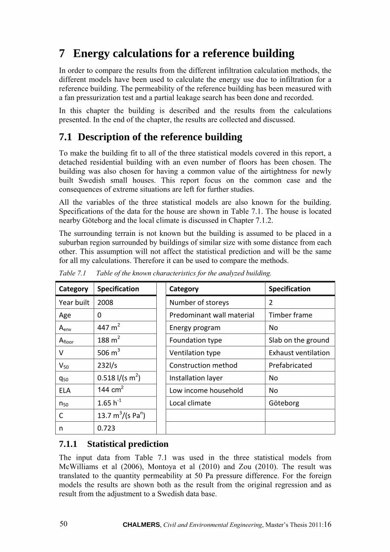
CHALMERS, Civil and Environmental Engineering, Master’s Thesis 2011:16 50
7 Energy calculations for a reference building In order to compare the results from the different infiltration calculation methods, the different models have been used to calculate the energy use due to infiltration for a reference building. The permeability of the reference building has been measured with a fan pressurization test and a partial leakage search has been done and recorded.
In this chapter the building is described and the results from the calculations presented. In the end of the chapter, the results are collected and discussed.
7.1 Description of the reference building
To make the building fit to all of the three statistical models covered in this report, a detached residential building with an even number of floors has been chosen. The building was also chosen for having a common value of the airtightness for newly built Swedish small houses. This report focus on the common case and the consequences of extreme situations are left for further studies.
All the variables of the three statistical models are also known for the building. Specifications of the data for the house are shown in Table 7.1. The house is located nearby Göteborg and the local climate is discussed in Chapter 7.1.2.
The surrounding terrain is not known but the building is assumed to be placed in a suburban region surrounded by buildings of similar size with some distance from each other. This assumption will not affect the statistical prediction and will be the same for all my calculations. Therefore it can be used to compare the methods.
Table 7.1 Table of the known characteristics for the analyzed building.
Category Specification Category Specification
Year built 2008 Number of storeys 2
Age 0 Predominant wall material Timber frame
Aenv 447 m2 Energy program No
Afloor 188 m2 Foundation type Slab on the ground
V 506 m3 Ventilation type Exhaust ventilation
V50 232l/s Construction method Prefabricated
q50 0.518 l/(s m2) Installation layer No
ELA 144 cm2 Low income household No
n50 1.65 h‐1 Local climate Göteborg
C 13.7 m3/(s Pan)
n 0.723
7.1.1 Statistical prediction
The input data from Table 7.1 was used in the three statistical models from McWilliams et al (2006), Montoya et al (2010) and Zou (2010). The result was translated to the quantity permeability at 50 Pa pressure difference. For the foreign models the results are shown both as the result from the original regression and as result from the adjustment to a Swedish data base.
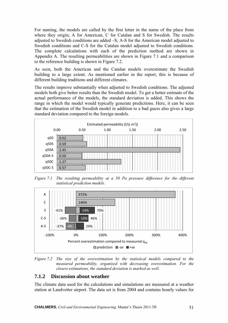
CHALMERS, Civil and Environmental Engineering, Master’s Thesis 2011:16 51
For naming, the models are called by the first letter in the name of the place from where they origin; A for American, C for Catalan and S for Swedish. The results adjusted to Swedish conditions are added –S; A-S for the American model adjusted to Swedish conditions and C-S for the Catalan model adjusted to Swedish conditions. The complete calculations with each of the prediction method are shown in Appendix A. The resulting permeabilities are shown in Figure 7.1 and a comparison to the reference building is shown in Figure 7.2.
As seen, both the American and the Catalan models overestimate the Swedish building to a large extent. As mentioned earlier in the report, this is because of different building traditions and different climates.
The results improve substantially when adjusted to Swedish conditions. The adjusted models both give better results than the Swedish model. To get a better estimate of the actual performance of the models, the standard deviation is added. This shows the range in which the model would typically generate predictions. Here, it can be seen that the estimation of the Swedish model in addition to a bad guess also gives a large standard deviation compared to the foreign models.
Figure 7.1 The resulting permeability at a 50 Pa pressure difference for the different
statistical prediction models.
Figure 7.2 The size of the overestimation by the statistical models compared to the
measured permeability, organized with decreasing overestimation. For the closest estimations, the standard deviation is marked as well.
7.1.2 Discussion about weather
The climate data used for the calculations and simulations are measured at a weather station at Landvetter airport. The data set is from 2004 and contains hourly values for
0.52
0.59
2.45
0.50
1.27
0.57
0.00 0.50 1.00 1.50 2.00 2.50
q50
q50S
q50A
q50A‐S
q50C
q50C‐S
Estimated permeability [l/(s m2)]
29%
46%
70%
‐37%
‐26%
‐41%
‐4%
10%
14%
146%
372%
‐100% 0% 100% 200% 300% 400%
A‐S
C‐S
S
C
A
Percent overestimation compared to measured q50
prediction ‐se +se
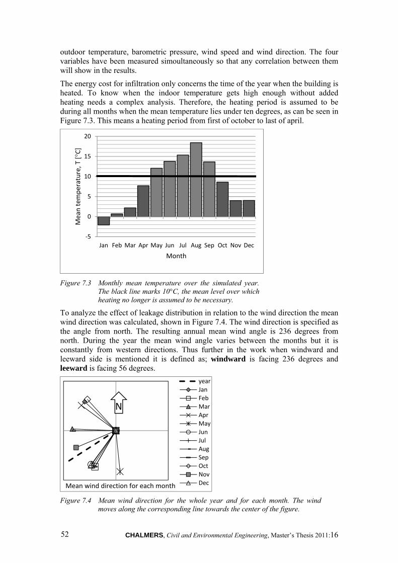
CHALMERS, Civil and Environmental Engineering, Master’s Thesis 2011:16 52
outdoor temperature, barometric pressure, wind speed and wind direction. The four variables have been measured simoultaneously so that any correlation between them will show in the results.
The energy cost for infiltration only concerns the time of the year when the building is heated. To know when the indoor temperature gets high enough without added heating needs a complex analysis. Therefore, the heating period is assumed to be during all months when the mean temperature lies under ten degrees, as can be seen in Figure 7.3. This means a heating period from first of october to last of april.
Figure 7.3 Monthly mean temperature over the simulated year.
The black line marks 10°C, the mean level over which heating no longer is assumed to be necessary.
To analyze the effect of leakage distribution in relation to the wind direction the mean wind direction was calculated, shown in Figure 7.4. The wind direction is specified as the angle from north. The resulting annual mean wind angle is 236 degrees from north. During the year the mean wind angle varies between the months but it is constantly from western directions. Thus further in the work when windward and leeward side is mentioned it is defined as; windward is facing 236 degrees and leeward is facing 56 degrees.
Figure 7.4 Mean wind direction for the whole year and for each month. The wind
moves along the corresponding line towards the center of the figure.
‐5
0
5
10
15
20
Jan Feb Mar Apr May Jun Jul Aug Sep Oct Nov Dec
Mean tem
perature, T [
°C]
Month
Mean wind direction for each month
year
Jan
Feb
Mar
Apr
May
Jun
Jul
Aug
Sep
Oct
Nov
Dec
N
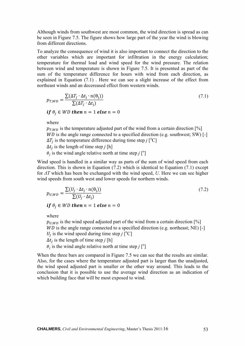
CHALMERS, Civil and Environmental Engineering, Master’s Thesis 2011:16 53
Although winds from southwest are most common, the wind direction is spread as can be seen in Figure 7.5. The figure shows how large part of the year the wind is blowing from different directions.
To analyze the consequence of wind it is also important to connect the direction to the other variables which are important for infiltration in the energy calculation; temperature for thermal load and wind speed for the wind pressure. The relation between wind and temperature is shown in Figure 7.5. It is presented as part of the sum of the temperature difference for hours with wind from each direction, as explained in Equation (7.1) . Here we can see a slight increase of the effect from northeast winds and an decereased effect from western winds.
,∑ ∆ ∙ Δ ∙ n θ
∑ ∆ ∙ Δ
(7.1)
∈ 1 0
where , is the temperature adjusted part of the wind from a certain direction [%]
is the angle range connected to a specified direction (e.g. southwest; SW) [-] ∆ is the temperature difference during time step j [oC] Δ is the length of time step j [h]
is the wind angle relative north at time step j [o]
Wind speed is handled in a similar way as parts of the sum of wind speed from each direction. This is shown in Equation (7.2) which is identical to Equation (7.1) except for ΔT which has been be exchanged with the wind speed, U. Here we can see higher wind speeds from south west and lower speeds for northern winds.
,∑ ∙ Δ ∙ n θ
∑ ∙ Δ
(7.2)
∈ 1 0
where , is the wind speed adjusted part of the wind from a certain direction [%]
is the angle range connected to a specified direction (e.g. northeast; NE) [-] is the wind speed during time step j [oC]
Δ is the length of time step j [h] is the wind angle relative north at time step j [o]
When the three bars are compared in Figure 7.5 we can see that the results are similar. Also, for the cases where the temperature adjusted part is larger than the unadjusted, the wind speed adjusted part is smaller or the other way around. This leads to the conclusion that it is possible to use the average wind direction as an indication of which building face that will be most exposed to wind.

CHALMERS, Civil and Environmental Engineering, Master’s Thesis 2011:16 54
Figure 7.5 The figure shows how large part of the year the wind blows from each direction.
It also shows the part of the temperature difference for wind blowing from each direction and the part of the wind speed in each direction.
Figure 7.6 shows the max and the mean wind speed for each month. It seems to be rather small differences over the year and the month with the higher max wind speed does not necessarily have higher mean wind speed.
Figure 7.6 The mean and max wind speed for each month.
7.2 The numerical simulation model To test the precision of the different calculation models, a simulation model was created in a numerical simulation software. Commonly, the known characteristics of a building is an airtightness parameter value, like q50, or the coefficients in the power law, C and n in Equation (3.13).
0%
2%
4%
6%
8%
10%
12%
14%
N NE E SE S SW W NW
Part of the year
Wind direction
Hours Temperature Wind speed
0
2
4
6
8
10
12
14
Jan Feb Mar Apr May Jun Jul Aug Sep Oct Nov Dec
Wind Speed, V
met [m
/s]
MonthMean Max
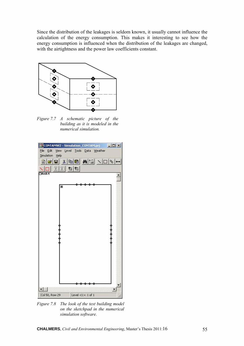
CHALMERS, Civil and Environmental Engineering, Master’s Thesis 2011:16 55
Since the distribution of the leakages is seldom known, it usually cannot influence the calculation of the energy consumption. This makes it interesting to see how the energy consumption is influenced when the distribution of the leakages are changed, with the airtightness and the power law coefficients constant.
Figure 7.7 A schematic picture of the
building as it is modeled in the numerical simulation.
Figure 7.8 The look of the test building model
on the sketchpad in the numerical simulation software.
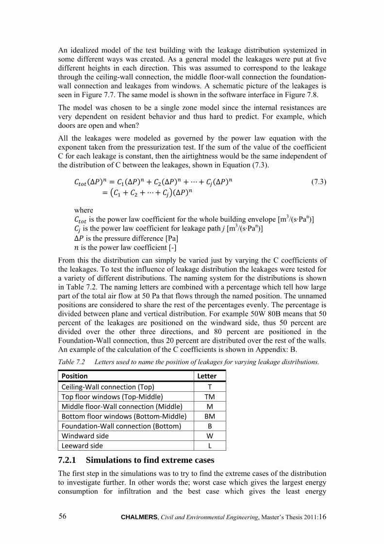
CHALMERS, Civil and Environmental Engineering, Master’s Thesis 2011:16 56
An idealized model of the test building with the leakage distribution systemized in some different ways was created. As a general model the leakages were put at five different heights in each direction. This was assumed to correspond to the leakage through the ceiling-wall connection, the middle floor-wall connection the foundation-wall connection and leakages from windows. A schematic picture of the leakages is seen in Figure 7.7. The same model is shown in the software interface in Figure 7.8.
The model was chosen to be a single zone model since the internal resistances are very dependent on resident behavior and thus hard to predict. For example, which doors are open and when?
All the leakages were modeled as governed by the power law equation with the exponent taken from the pressurization test. If the sum of the value of the coefficient C for each leakage is constant, then the airtightness would be the same independent of the distribution of C between the leakages, shown in Equation (7.3).
∆ ∆ ∆ ⋯ ∆⋯ ∆
(7.3)
where is the power law coefficient for the whole building envelope [m3/(s·Pan)]
is the power law coefficient for leakage path j [m3/(s·Pan)] ∆ is the pressure difference [Pa]
is the power law coefficient [-]
From this the distribution can simply be varied just by varying the C coefficients of the leakages. To test the influence of leakage distribution the leakages were tested for a variety of different distributions. The naming system for the distributions is shown in Table 7.2. The naming letters are combined with a percentage which tell how large part of the total air flow at 50 Pa that flows through the named position. The unnamed positions are considered to share the rest of the percentages evenly. The percentage is divided between plane and vertical distribution. For example 50W 80B means that 50 percent of the leakages are positioned on the windward side, thus 50 percent are divided over the other three directions, and 80 percent are positioned in the Foundation-Wall connection, thus 20 percent are distributed over the rest of the walls. An example of the calculation of the C coefficients is shown in Appendix: B.
Table 7.2 Letters used to name the position of leakages for varying leakage distributions.
Position Letter
Ceiling‐Wall connection (Top) T
Top floor windows (Top‐Middle) TM
Middle floor‐Wall connection (Middle) M
Bottom floor windows (Bottom‐Middle) BM
Foundation‐Wall connection (Bottom) B
Windward side W
Leeward side L
7.2.1 Simulations to find extreme cases
The first step in the simulations was to try to find the extreme cases of the distribution to investigate further. In other words the; worst case which gives the largest energy consumption for infiltration and the best case which gives the least energy
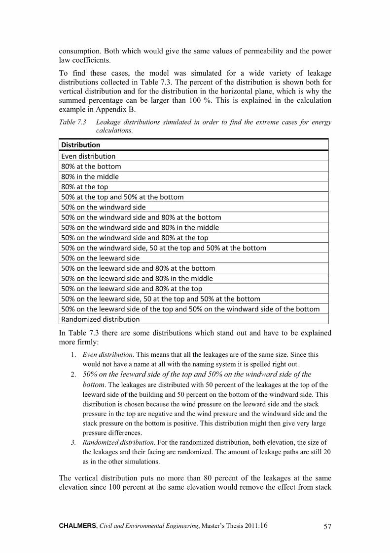
CHALMERS, Civil and Environmental Engineering, Master’s Thesis 2011:16 57
consumption. Both which would give the same values of permeability and the power law coefficients.
To find these cases, the model was simulated for a wide variety of leakage distributions collected in Table 7.3. The percent of the distribution is shown both for vertical distribution and for the distribution in the horizontal plane, which is why the summed percentage can be larger than 100 %. This is explained in the calculation example in Appendix B.
Table 7.3 Leakage distributions simulated in order to find the extreme cases for energy calculations.
Distribution
Even distribution
80% at the bottom
80% in the middle
80% at the top
50% at the top and 50% at the bottom
50% on the windward side
50% on the windward side and 80% at the bottom
50% on the windward side and 80% in the middle
50% on the windward side and 80% at the top
50% on the windward side, 50 at the top and 50% at the bottom
50% on the leeward side
50% on the leeward side and 80% at the bottom
50% on the leeward side and 80% in the middle
50% on the leeward side and 80% at the top
50% on the leeward side, 50 at the top and 50% at the bottom
50% on the leeward side of the top and 50% on the windward side of the bottom
Randomized distribution
In Table 7.3 there are some distributions which stand out and have to be explained more firmly:
1. Even distribution. This means that all the leakages are of the same size. Since this would not have a name at all with the naming system it is spelled right out.
2. 50% on the leeward side of the top and 50% on the windward side of the bottom. The leakages are distributed with 50 percent of the leakages at the top of the leeward side of the building and 50 percent on the bottom of the windward side. This distribution is chosen because the wind pressure on the leeward side and the stack pressure in the top are negative and the wind pressure and the windward side and the stack pressure on the bottom is positive. This distribution might then give very large pressure differences.
3. Randomized distribution. For the randomized distribution, both elevation, the size of the leakages and their facing are randomized. The amount of leakage paths are still 20 as in the other simulations.
The vertical distribution puts no more than 80 percent of the leakages at the same elevation since 100 percent at the same elevation would remove the effect from stack
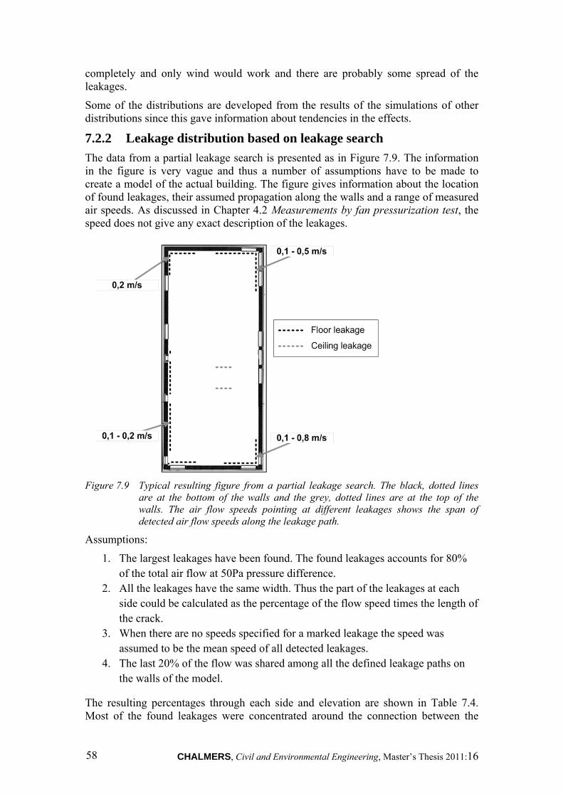
CHALMERS, Civil and Environmental Engineering, Master’s Thesis 2011:16 58
completely and only wind would work and there are probably some spread of the leakages.
Some of the distributions are developed from the results of the simulations of other distributions since this gave information about tendencies in the effects.
7.2.2 Leakage distribution based on leakage search
The data from a partial leakage search is presented as in Figure 7.9. The information in the figure is very vague and thus a number of assumptions have to be made to create a model of the actual building. The figure gives information about the location of found leakages, their assumed propagation along the walls and a range of measured air speeds. As discussed in Chapter 4.2 Measurements by fan pressurization test, the speed does not give any exact description of the leakages.
Figure 7.9 Typical resulting figure from a partial leakage search. The black, dotted lines
are at the bottom of the walls and the grey, dotted lines are at the top of the walls. The air flow speeds pointing at different leakages shows the span of detected air flow speeds along the leakage path.
Assumptions:
1. The largest leakages have been found. The found leakages accounts for 80% of the total air flow at 50Pa pressure difference.
2. All the leakages have the same width. Thus the part of the leakages at each side could be calculated as the percentage of the flow speed times the length of the crack.
3. When there are no speeds specified for a marked leakage the speed was assumed to be the mean speed of all detected leakages.
4. The last 20% of the flow was shared among all the defined leakage paths on the walls of the model.
The resulting percentages through each side and elevation are shown in Table 7.4. Most of the found leakages were concentrated around the connection between the
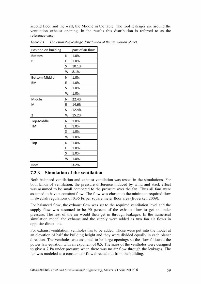
CHALMERS, Civil and Environmental Engineering, Master’s Thesis 2011:16 59
second floor and the wall, the Middle in the table. The roof leakages are around the ventilation exhaust opening. In the results this distribution is referred to as the reference case.
Table 7.4 The estimated leakage distribution of the simulation object.
Position on building part of air flow
Bottom N 1.0%
B E 1.0%
S 10.1%
W 8.1%
Bottom‐Middle N 1.0%
BM E 1.0%
S 1.0%
W 1.0%
Middle N 22.4%
M E 14.6%
S 12.4%
2 W 15.2%
Top‐Middle N 1.0%
TM E 1.0%
S 1.0%
W 1.0%
Top N 1.0%
T E 1.0%
S 1.0%
W 1.0%
Roof 3.2%
7.2.3 Simulation of the ventilation
Both balanced ventilation and exhaust ventilation was tested in the simulations. For both kinds of ventilation, the pressure difference induced by wind and stack effect was assumed to be small compared to the pressure over the fan. Thus all fans were assumed to have a constant flow. The flow was chosen to the minimum required flow in Swedish regulations of 0.35 l/s per square meter floor area (Boverket, 2009).
For balanced flow, the exhaust flow was set to the required ventilation level and the supply flow was assumed to be 90 percent of the exhaust flow to get an under pressure. The rest of the air would then get in through leakages. In the numerical simulation model the exhaust and the supply were added as two fan air flows in opposite directions.
For exhaust ventilation, ventholes has to be added. Those were put into the model at an elevation of half the building height and they were divided equally in each planar direction. The ventholes was assumed to be large openings so the flow followed the power law equation with an exponent of 0.5. The sizes of the ventholes were designed to give a 7 Pa under pressure when there was no air flow through the leakages. The fan was modeled as a constant air flow directed out from the building.
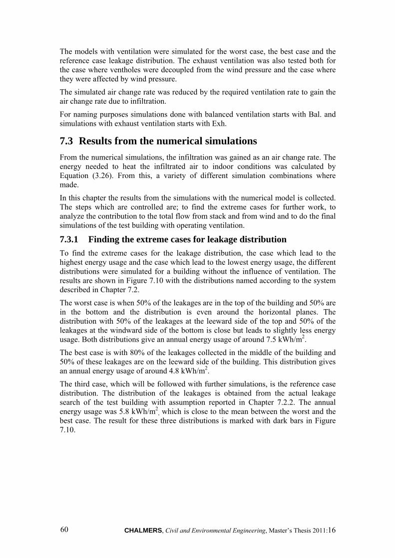
CHALMERS, Civil and Environmental Engineering, Master’s Thesis 2011:16 60
The models with ventilation were simulated for the worst case, the best case and the reference case leakage distribution. The exhaust ventilation was also tested both for the case where ventholes were decoupled from the wind pressure and the case where they were affected by wind pressure.
The simulated air change rate was reduced by the required ventilation rate to gain the air change rate due to infiltration.
For naming purposes simulations done with balanced ventilation starts with Bal. and simulations with exhaust ventilation starts with Exh.
7.3 Results from the numerical simulations
From the numerical simulations, the infiltration was gained as an air change rate. The energy needed to heat the infiltrated air to indoor conditions was calculated by Equation (3.26). From this, a variety of different simulation combinations where made.
In this chapter the results from the simulations with the numerical model is collected. The steps which are controlled are; to find the extreme cases for further work, to analyze the contribution to the total flow from stack and from wind and to do the final simulations of the test building with operating ventilation.
7.3.1 Finding the extreme cases for leakage distribution
To find the extreme cases for the leakage distribution, the case which lead to the highest energy usage and the case which lead to the lowest energy usage, the different distributions were simulated for a building without the influence of ventilation. The results are shown in Figure 7.10 with the distributions named according to the system described in Chapter 7.2.
The worst case is when 50% of the leakages are in the top of the building and 50% are in the bottom and the distribution is even around the horizontal planes. The distribution with 50% of the leakages at the leeward side of the top and 50% of the leakages at the windward side of the bottom is close but leads to slightly less energy usage. Both distributions give an annual energy usage of around 7.5 kWh/m2.
The best case is with 80% of the leakages collected in the middle of the building and 50% of these leakages are on the leeward side of the building. This distribution gives an annual energy usage of around 4.8 kWh/m2.
The third case, which will be followed with further simulations, is the reference case distribution. The distribution of the leakages is obtained from the actual leakage search of the test building with assumption reported in Chapter 7.2.2. The annual energy usage was 5.8 kWh/m2
, which is close to the mean between the worst and the best case. The result for these three distributions is marked with dark bars in Figure 7.10.
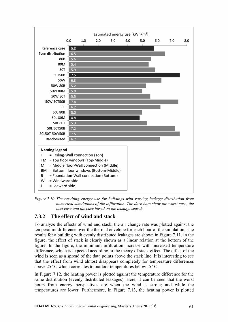
CHALMERS, Civil and Environmental Engineering, Master’s Thesis 2011:16 61
Figure 7.10 The resulting energy use for buildings with varying leakage distribution from
numerical simulations of the infiltration. The dark bars show the worst case, the best case and the case based on the leakage search.
7.3.2 The effect of wind and stack
To analyze the effects of wind and stack, the air change rate was plotted against the temperature difference over the thermal envelope for each hour of the simulation. The results for a building with evenly distributed leakages are shown in Figure 7.11. In the figure, the effect of stack is clearly shown as a linear relation at the bottom of the figure. In the figure, the minimum infiltration increase with increased temperature difference, which is expected according to the theory of stack effect. The effect of the wind is seen as a spread of the data points above the stack line. It is interesting to see that the effect from wind almost disappears completely for temperature differences above 25 °C which correlates to outdoor temperatures below -5 °C.
In Figure 7.12, the heating power is plotted against the temperature difference for the same distribution (evenly distributed leakages). Here, it can be seen that the worst hours from energy perspectives are when the wind is strong and while the temperatures are lower. Furthermore, in Figure 7.13, the heating power is plotted
5.8
6.5
5.6
5.4
5.9
7.5
6.3
5.2
5.0
5.5
7.4
6.2
5.0
4.8
5.3
7.2
7.5
6.2
0.0 1.0 2.0 3.0 4.0 5.0 6.0 7.0 8.0
Reference case
Even distribution
80B
80M
80T
50T50B
50W
50W 80B
50W 80M
50W 80T
50W 50T50B
50L
50L 80B
50L 80M
50L 80T
50L 50T50B
50L50T‐50W50B
Randomized
Estimated energy use [kWh/m2]
Naming legendT = Ceiling‐Wall connection (Top)TM = Top floor windows (Top‐Middle)M = Middle floor‐Wall connection (Middle)BM = Bottom floor windows (Bottom‐Middle)B = Foundation‐Wall connection (Bottom)W = Windward sideL = Leeward side
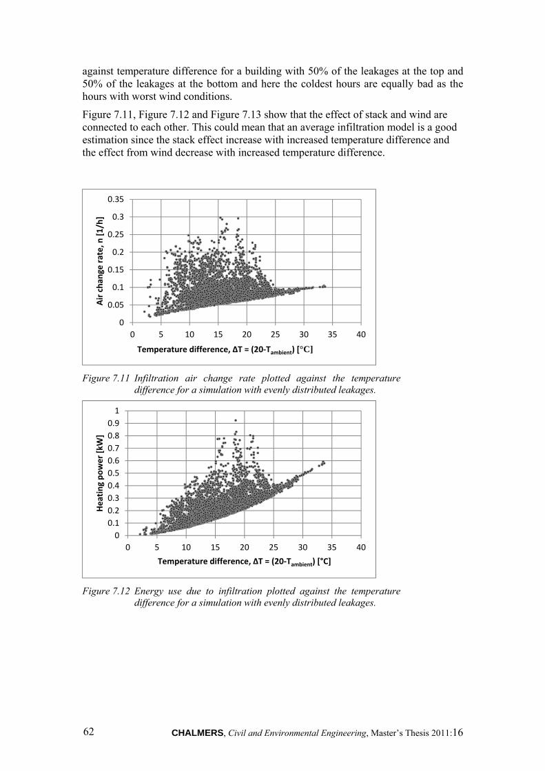
CHALMERS, Civil and Environmental Engineering, Master’s Thesis 2011:16 62
against temperature difference for a building with 50% of the leakages at the top and 50% of the leakages at the bottom and here the coldest hours are equally bad as the hours with worst wind conditions.
Figure 7.11, Figure 7.12 and Figure 7.13 show that the effect of stack and wind are connected to each other. This could mean that an average infiltration model is a good estimation since the stack effect increase with increased temperature difference and the effect from wind decrease with increased temperature difference.
Figure 7.11 Infiltration air change rate plotted against the temperature
difference for a simulation with evenly distributed leakages.
Figure 7.12 Energy use due to infiltration plotted against the temperature
difference for a simulation with evenly distributed leakages.
0
0.05
0.1
0.15
0.2
0.25
0.3
0.35
0 5 10 15 20 25 30 35 40
Air chan
ge rate, n
[1/h]
Temperature difference, ΔT = (20‐Tambient) [°C]
0
0.1
0.2
0.3
0.4
0.5
0.6
0.7
0.8
0.9
1
0 5 10 15 20 25 30 35 40
Heating power [kW]
Temperature difference, ΔT = (20‐Tambient) [°C]
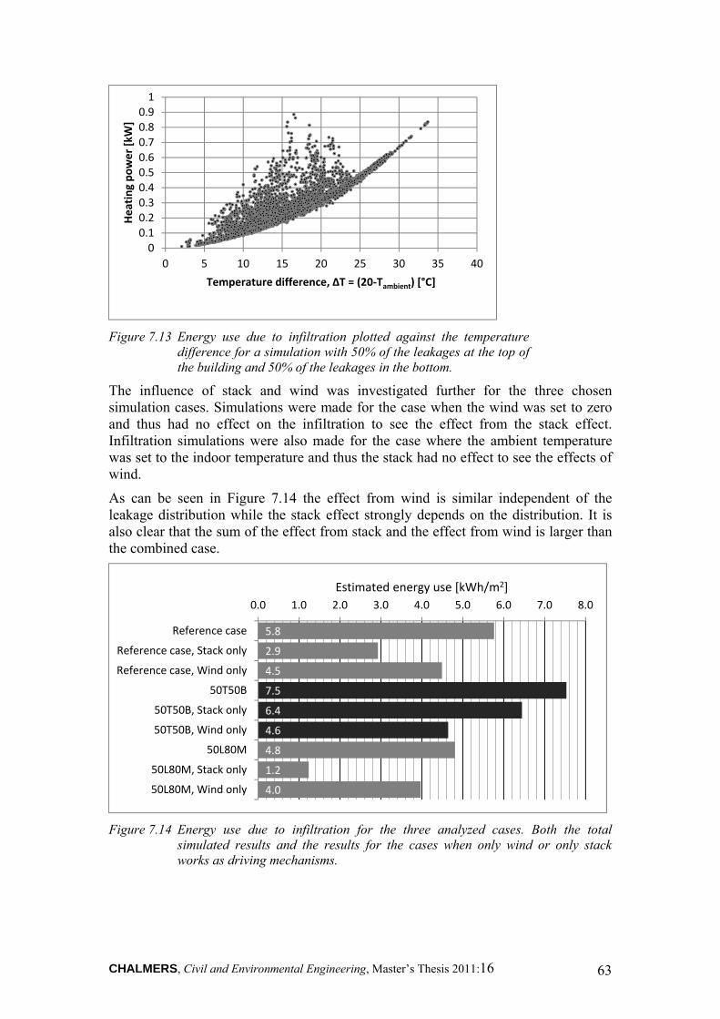
CHALMERS, Civil and Environmental Engineering, Master’s Thesis 2011:16 63
Figure 7.13 Energy use due to infiltration plotted against the temperature
difference for a simulation with 50% of the leakages at the top of the building and 50% of the leakages in the bottom.
The influence of stack and wind was investigated further for the three chosen simulation cases. Simulations were made for the case when the wind was set to zero and thus had no effect on the infiltration to see the effect from the stack effect. Infiltration simulations were also made for the case where the ambient temperature was set to the indoor temperature and thus the stack had no effect to see the effects of wind.
As can be seen in Figure 7.14 the effect from wind is similar independent of the leakage distribution while the stack effect strongly depends on the distribution. It is also clear that the sum of the effect from stack and the effect from wind is larger than the combined case.
Figure 7.14 Energy use due to infiltration for the three analyzed cases. Both the total
simulated results and the results for the cases when only wind or only stack works as driving mechanisms.
00.10.20.30.40.50.60.70.80.91
0 5 10 15 20 25 30 35 40
Heating power [kW]
Temperature difference, ΔT = (20‐Tambient) [°C]
5.8
2.9
4.5
7.5
6.4
4.6
4.8
1.2
4.0
0.0 1.0 2.0 3.0 4.0 5.0 6.0 7.0 8.0
Reference case
Reference case, Stack only
Reference case, Wind only
50T50B
50T50B, Stack only
50T50B, Wind only
50L80M
50L80M, Stack only
50L80M, Wind only
Estimated energy use [kWh/m2]
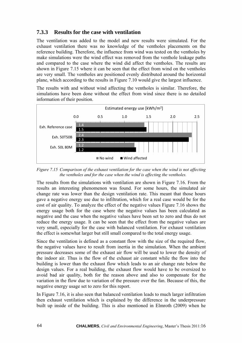
CHALMERS, Civil and Environmental Engineering, Master’s Thesis 2011:16 64
7.3.3 Results for the case with ventilation
The ventilation was added to the model and new results were simulated. For the exhaust ventilation there was no knowledge of the ventholes placements on the reference building. Therefore, the influence from wind was tested on the ventholes by make simulations were the wind effect was removed from the venthole leakage paths and compared to the case where the wind did affect the ventholes. The results are shown in Figure 7.15 where it can be seen that the effect from wind on the ventholes are very small. The ventholes are positioned evenly distributed around the horizontal plane, which according to the results in Figure 7.10 would give the largest influence.
The results with and without wind affecting the ventholes is similar. Therefore, the simulations have been done without the effect from wind since there is no detailed information of their position.
Figure 7.15 Comparison of the exhaust ventilation for the case when the wind is not affecting
the ventholes and for the case when the wind is affecting the ventholes.
The results from the simulations with ventilation are shown in Figure 7.16. From the results an interesting phenomenon was found. For some hours, the simulated air change rate was lower than the design ventilation rate. This meant that those hours gave a negative energy use due to infiltration, which for a real case would be for the cost of air quality. To analyze the effect of the negative values Figure 7.16 shows the energy usage both for the case where the negative values has been calculated as negative and the case when the negative values have been set to zero and thus do not reduce the energy usage. It can be seen that the effect from the negative values are very small, especially for the case with balanced ventilation. For exhaust ventilation the effect is somewhat larger but still small compared to the total energy usage.
Since the ventilation is defined as a constant flow with the size of the required flow, the negative values have to result from inertia in the simulation. When the ambient pressure decreases some of the exhaust air flow will be used to lower the density of the indoor air. Thus is the flow of the exhaust air constant while the flow into the building is lower than the exhaust flow which leads to an air change rate below the design values. For a real building, the exhaust flow would have to be oversized to avoid bad air quality, both for the reason above and also to compensate for the variation in the flow due to variation of the pressure over the fan. Because of this, the negative energy usage set to zero for this report.
In Figure 7.16, it is also seen that balanced ventilation leads to much larger infiltration then exhaust ventilation which is explained by the difference in the underpressure built up inside of the building. This is also mentioned in Elmroth (2009) when he
1.4
2.4
1.2
1.5
2.3
1.2
0.0 0.5 1.0 1.5 2.0 2.5
Exh. Reference case
Exh. 50T50B
Exh. 50L 80M
Estimated energy use [kWh/m2]
No wind Wind affected
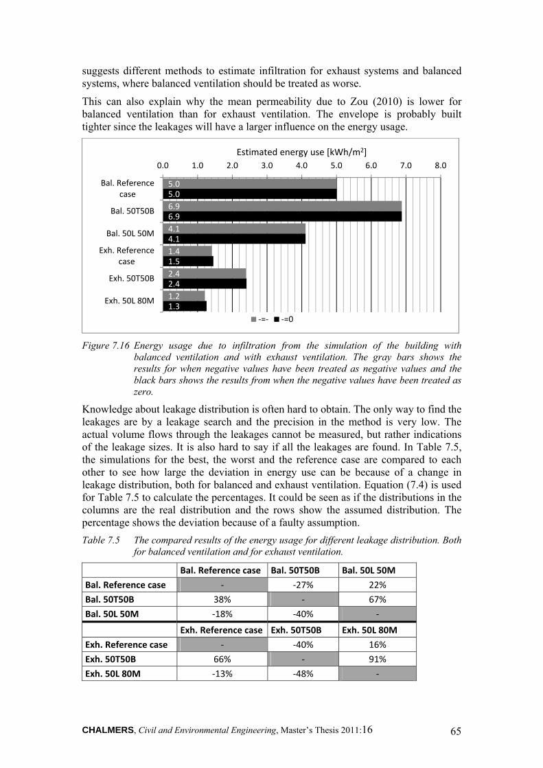
CHALMERS, Civil and Environmental Engineering, Master’s Thesis 2011:16 65
suggests different methods to estimate infiltration for exhaust systems and balanced systems, where balanced ventilation should be treated as worse.
This can also explain why the mean permeability due to Zou (2010) is lower for balanced ventilation than for exhaust ventilation. The envelope is probably built tighter since the leakages will have a larger influence on the energy usage.
Figure 7.16 Energy usage due to infiltration from the simulation of the building with
balanced ventilation and with exhaust ventilation. The gray bars shows the results for when negative values have been treated as negative values and the black bars shows the results from when the negative values have been treated as zero.
Knowledge about leakage distribution is often hard to obtain. The only way to find the leakages are by a leakage search and the precision in the method is very low. The actual volume flows through the leakages cannot be measured, but rather indications of the leakage sizes. It is also hard to say if all the leakages are found. In Table 7.5, the simulations for the best, the worst and the reference case are compared to each other to see how large the deviation in energy use can be because of a change in leakage distribution, both for balanced and exhaust ventilation. Equation (7.4) is used for Table 7.5 to calculate the percentages. It could be seen as if the distributions in the columns are the real distribution and the rows show the assumed distribution. The percentage shows the deviation because of a faulty assumption.
Table 7.5 The compared results of the energy usage for different leakage distribution. Both for balanced ventilation and for exhaust ventilation.
Bal. Reference case Bal. 50T50B Bal. 50L 50M
Bal. Reference case ‐ ‐27% 22%
Bal. 50T50B 38% ‐ 67%
Bal. 50L 50M ‐18% ‐40% ‐
Exh. Reference case Exh. 50T50B Exh. 50L 80M
Exh. Reference case ‐ ‐40% 16%
Exh. 50T50B 66% ‐ 91%
Exh. 50L 80M ‐13% ‐48% ‐
5.0
6.9
4.1
1.4
2.4
1.2
5.0
6.9
4.1
1.5
2.4
1.3
0.0 1.0 2.0 3.0 4.0 5.0 6.0 7.0 8.0
Bal. Referencecase
Bal. 50T50B
Bal. 50L 50M
Exh. Referencecase
Exh. 50T50B
Exh. 50L 80M
Estimated energy use [kWh/m2]
‐=‐ ‐=0
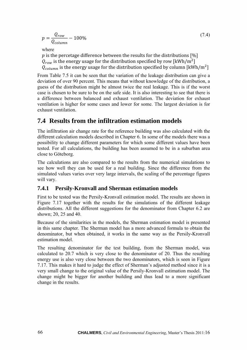
CHALMERS, Civil and Environmental Engineering, Master’s Thesis 2011:16 66
100%
(7.4)
where isthepercetagedifferencebetween the results for the distributions %
istheenergyusageforthe distribution specified by row kWh/m istheenergyusagefor the distribution specified by column kWh/m
From Table 7.5 it can be seen that the variation of the leakage distribution can give a deviation of over 90 percent. This means that without knowledge of the distribution, a guess of the distribution might be almost twice the real leakage. This is if the worst case is chosen to be sure to be on the safe side. It is also interesting to see that there is a difference between balanced and exhaust ventilation. The deviation for exhaust ventilation is higher for some cases and lower for some. The largest deviation is for exhaust ventilation.
7.4 Results from the infiltration estimation models
The infiltration air change rate for the reference building was also calculated with the different calculation models described in Chapter 6. In some of the models there was a possibility to change different parameters for which some different values have been tested. For all calculations, the building has been assumed to be in a suburban area close to Göteborg.
The calculations are also compared to the results from the numerical simulations to see how well they can be used for a real building. Since the difference from the simulated values varies over very large intervals, the scaling of the percentage figures will vary.
7.4.1 Persily-Kronvall and Sherman estimation models
First to be tested was the Persily-Kronvall estimation model. The results are shown in Figure 7.17 together with the results for the simulations of the different leakage distributions. All the different suggestions for the denominator from Chapter 6.2 are shown; 20, 25 and 40.
Because of the similarities in the models, the Sherman estimation model is presented in this same chapter. The Sherman model has a more advanced formula to obtain the denominator, but when obtained, it works in the same way as the Persily-Kronvall estimation model.
The resulting denominator for the test building, from the Sherman model, was calculated to 20.7 which is very close to the denominator of 20. Thus the resulting energy use is also very close between the two denominators, which is seen in Figure 7.17. This makes it hard to judge the effect of Sherman’s adjusted method since it is a very small change to the original value of the Persily-Kronvall estimation model. The change might be bigger for another building and thus lead to a more significant change in the results.
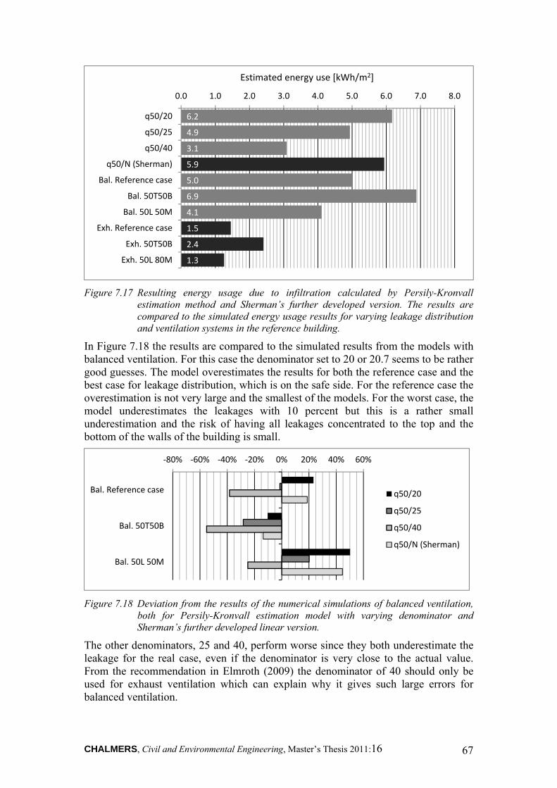
CHALMERS, Civil and Environmental Engineering, Master’s Thesis 2011:16 67
Figure 7.17 Resulting energy usage due to infiltration calculated by Persily-Kronvall
estimation method and Sherman’s further developed version. The results are compared to the simulated energy usage results for varying leakage distribution and ventilation systems in the reference building.
In Figure 7.18 the results are compared to the simulated results from the models with balanced ventilation. For this case the denominator set to 20 or 20.7 seems to be rather good guesses. The model overestimates the results for both the reference case and the best case for leakage distribution, which is on the safe side. For the reference case the overestimation is not very large and the smallest of the models. For the worst case, the model underestimates the leakages with 10 percent but this is a rather small underestimation and the risk of having all leakages concentrated to the top and the bottom of the walls of the building is small.
Figure 7.18 Deviation from the results of the numerical simulations of balanced ventilation,
both for Persily-Kronvall estimation model with varying denominator and Sherman’s further developed linear version.
The other denominators, 25 and 40, perform worse since they both underestimate the leakage for the real case, even if the denominator is very close to the actual value. From the recommendation in Elmroth (2009) the denominator of 40 should only be used for exhaust ventilation which can explain why it gives such large errors for balanced ventilation.
6.2
4.9
3.1
5.9
5.0
6.9
4.1
1.5
2.4
1.3
0.0 1.0 2.0 3.0 4.0 5.0 6.0 7.0 8.0
q50/20
q50/25
q50/40
q50/N (Sherman)
Bal. Reference case
Bal. 50T50B
Bal. 50L 50M
Exh. Reference case
Exh. 50T50B
Exh. 50L 80M
Estimated energy use [kWh/m2]
‐80% ‐60% ‐40% ‐20% 0% 20% 40% 60%
Bal. Reference case
Bal. 50T50B
Bal. 50L 50M
q50/20
q50/25
q50/40
q50/N (Sherman)
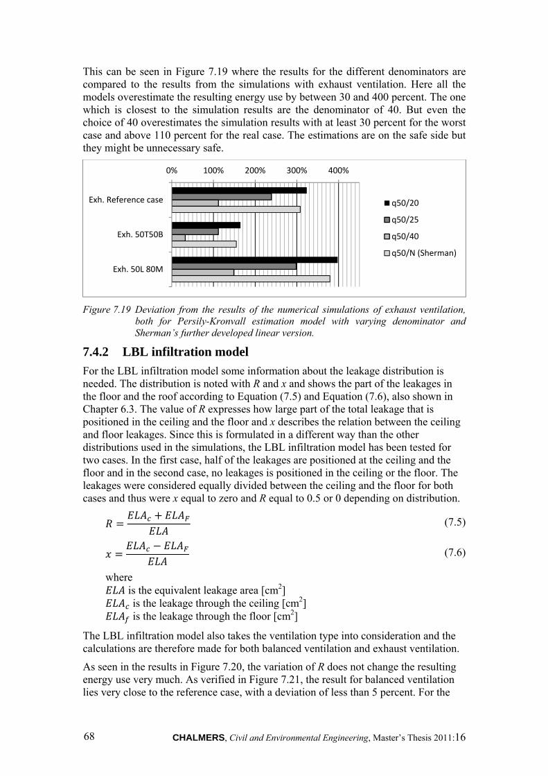
CHALMERS, Civil and Environmental Engineering, Master’s Thesis 2011:16 68
This can be seen in Figure 7.19 where the results for the different denominators are compared to the results from the simulations with exhaust ventilation. Here all the models overestimate the resulting energy use by between 30 and 400 percent. The one which is closest to the simulation results are the denominator of 40. But even the choice of 40 overestimates the simulation results with at least 30 percent for the worst case and above 110 percent for the real case. The estimations are on the safe side but they might be unnecessary safe.
Figure 7.19 Deviation from the results of the numerical simulations of exhaust ventilation,
both for Persily-Kronvall estimation model with varying denominator and Sherman’s further developed linear version.
7.4.2 LBL infiltration model
For the LBL infiltration model some information about the leakage distribution is needed. The distribution is noted with R and x and shows the part of the leakages in the floor and the roof according to Equation (7.5) and Equation (7.6), also shown in Chapter 6.3. The value of R expresses how large part of the total leakage that is positioned in the ceiling and the floor and x describes the relation between the ceiling and floor leakages. Since this is formulated in a different way than the other distributions used in the simulations, the LBL infiltration model has been tested for two cases. In the first case, half of the leakages are positioned at the ceiling and the floor and in the second case, no leakages is positioned in the ceiling or the floor. The leakages were considered equally divided between the ceiling and the floor for both cases and thus were x equal to zero and R equal to 0.5 or 0 depending on distribution.
(7.5)
(7.6)
where
is the equivalent leakage area [cm2] is the leakage through the ceiling [cm2] is the leakage through the floor [cm2]
The LBL infiltration model also takes the ventilation type into consideration and the calculations are therefore made for both balanced ventilation and exhaust ventilation.
As seen in the results in Figure 7.20, the variation of R does not change the resulting energy use very much. As verified in Figure 7.21, the result for balanced ventilation lies very close to the reference case, with a deviation of less than 5 percent. For the
0% 100% 200% 300% 400%
Exh. Reference case
Exh. 50T50B
Exh. 50L 80M
q50/20
q50/25
q50/40
q50/N (Sherman)
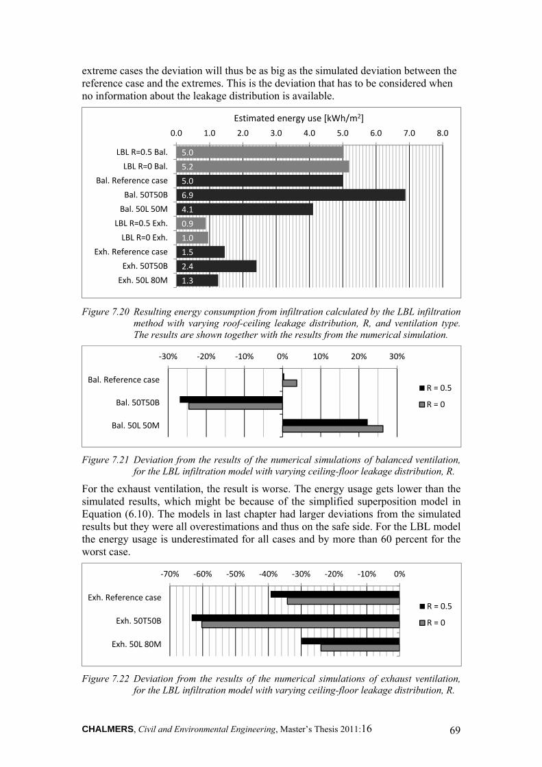
CHALMERS, Civil and Environmental Engineering, Master’s Thesis 2011:16 69
extreme cases the deviation will thus be as big as the simulated deviation between the reference case and the extremes. This is the deviation that has to be considered when no information about the leakage distribution is available.
Figure 7.20 Resulting energy consumption from infiltration calculated by the LBL infiltration
method with varying roof-ceiling leakage distribution, R, and ventilation type. The results are shown together with the results from the numerical simulation.
Figure 7.21 Deviation from the results of the numerical simulations of balanced ventilation,
for the LBL infiltration model with varying ceiling-floor leakage distribution, R.
For the exhaust ventilation, the result is worse. The energy usage gets lower than the simulated results, which might be because of the simplified superposition model in Equation (6.10). The models in last chapter had larger deviations from the simulated results but they were all overestimations and thus on the safe side. For the LBL model the energy usage is underestimated for all cases and by more than 60 percent for the worst case.
Figure 7.22 Deviation from the results of the numerical simulations of exhaust ventilation,
for the LBL infiltration model with varying ceiling-floor leakage distribution, R.
5.0
5.2
5.0
6.9
4.1
0.9
1.0
1.5
2.4
1.3
0.0 1.0 2.0 3.0 4.0 5.0 6.0 7.0 8.0
LBL R=0.5 Bal.
LBL R=0 Bal.
Bal. Reference case
Bal. 50T50B
Bal. 50L 50M
LBL R=0.5 Exh.
LBL R=0 Exh.
Exh. Reference case
Exh. 50T50B
Exh. 50L 80M
Estimated energy use [kWh/m2]
‐30% ‐20% ‐10% 0% 10% 20% 30%
Bal. Reference case
Bal. 50T50B
Bal. 50L 50M
R = 0.5
R = 0
‐70% ‐60% ‐50% ‐40% ‐30% ‐20% ‐10% 0%
Exh. Reference case
Exh. 50T50B
Exh. 50L 80M
R = 0.5
R = 0
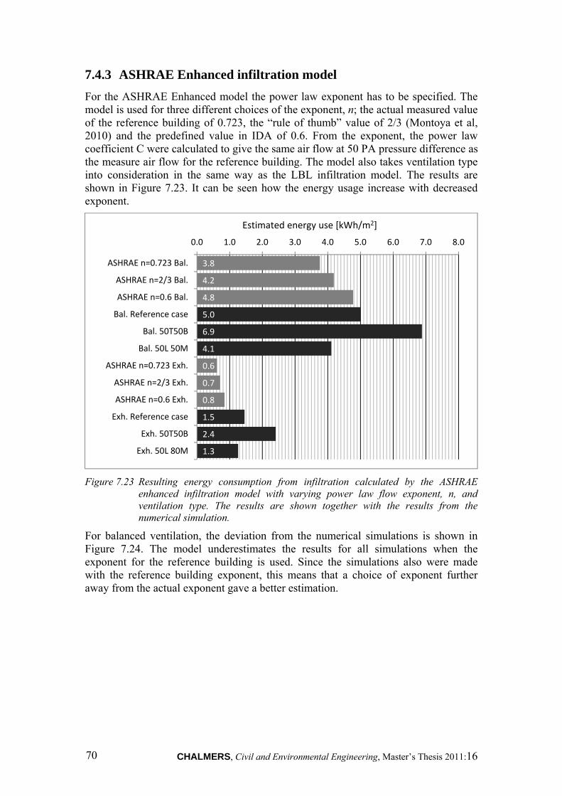
CHALMERS, Civil and Environmental Engineering, Master’s Thesis 2011:16 70
7.4.3 ASHRAE Enhanced infiltration model
For the ASHRAE Enhanced model the power law exponent has to be specified. The model is used for three different choices of the exponent, n; the actual measured value of the reference building of 0.723, the “rule of thumb” value of 2/3 (Montoya et al, 2010) and the predefined value in IDA of 0.6. From the exponent, the power law coefficient C were calculated to give the same air flow at 50 PA pressure difference as the measure air flow for the reference building. The model also takes ventilation type into consideration in the same way as the LBL infiltration model. The results are shown in Figure 7.23. It can be seen how the energy usage increase with decreased exponent.
Figure 7.23 Resulting energy consumption from infiltration calculated by the ASHRAE
enhanced infiltration model with varying power law flow exponent, n, and ventilation type. The results are shown together with the results from the numerical simulation.
For balanced ventilation, the deviation from the numerical simulations is shown in Figure 7.24. The model underestimates the results for all simulations when the exponent for the reference building is used. Since the simulations also were made with the reference building exponent, this means that a choice of exponent further away from the actual exponent gave a better estimation.
3.8
4.2
4.8
5.0
6.9
4.1
0.6
0.7
0.8
1.5
2.4
1.3
0.0 1.0 2.0 3.0 4.0 5.0 6.0 7.0 8.0
ASHRAE n=0.723 Bal.
ASHRAE n=2/3 Bal.
ASHRAE n=0.6 Bal.
Bal. Reference case
Bal. 50T50B
Bal. 50L 50M
ASHRAE n=0.723 Exh.
ASHRAE n=2/3 Exh.
ASHRAE n=0.6 Exh.
Exh. Reference case
Exh. 50T50B
Exh. 50L 80M
Estimated energy use [kWh/m2]
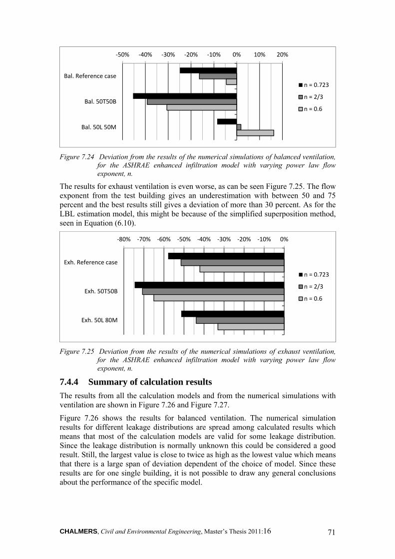
CHALMERS, Civil and Environmental Engineering, Master’s Thesis 2011:16 71
Figure 7.24 Deviation from the results of the numerical simulations of balanced ventilation,
for the ASHRAE enhanced infiltration model with varying power law flow exponent, n.
The results for exhaust ventilation is even worse, as can be seen Figure 7.25. The flow exponent from the test building gives an underestimation with between 50 and 75 percent and the best results still gives a deviation of more than 30 percent. As for the LBL estimation model, this might be because of the simplified superposition method, seen in Equation (6.10).
Figure 7.25 Deviation from the results of the numerical simulations of exhaust ventilation,
for the ASHRAE enhanced infiltration model with varying power law flow exponent, n.
7.4.4 Summary of calculation results
The results from all the calculation models and from the numerical simulations with ventilation are shown in Figure 7.26 and Figure 7.27.
Figure 7.26 shows the results for balanced ventilation. The numerical simulation results for different leakage distributions are spread among calculated results which means that most of the calculation models are valid for some leakage distribution. Since the leakage distribution is normally unknown this could be considered a good result. Still, the largest value is close to twice as high as the lowest value which means that there is a large span of deviation dependent of the choice of model. Since these results are for one single building, it is not possible to draw any general conclusions about the performance of the specific model.
‐50% ‐40% ‐30% ‐20% ‐10% 0% 10% 20%
Bal. Reference case
Bal. 50T50B
Bal. 50L 50M
n = 0.723
n = 2/3
n = 0.6
‐80% ‐70% ‐60% ‐50% ‐40% ‐30% ‐20% ‐10% 0%
Exh. Reference case
Exh. 50T50B
Exh. 50L 80M
n = 0.723
n = 2/3
n = 0.6
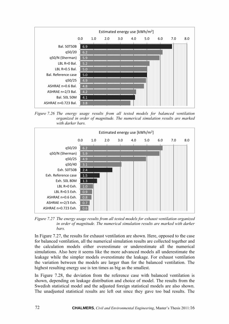
CHALMERS, Civil and Environmental Engineering, Master’s Thesis 2011:16 72
Figure 7.26 The energy usage results from all tested models for balanced ventilation
organized in order of magnitude. The numerical simulation results are marked with darker bars.
Figure 7.27 The energy usage results from all tested models for exhaust ventilation organized
in order of magnitude. The numerical simulation results are marked with darker bars.
In Figure 7.27, the results for exhaust ventilation are shown. Here, opposed to the case for balanced ventilation, all the numerical simulation results are collected together and the calculation models either overestimate or underestimate all the numerical simulations. Also here it seems like the more advanced models all underestimate the leakage while the simpler models overestimate the leakage. For exhaust ventilation the variation between the models are larger than for the balanced ventilation. The highest resulting energy use is ten times as big as the smallest.
In Figure 7.28, the deviation from the reference case with balanced ventilation is shown, depending on leakage distribution and choice of model. The results from the Swedish statistical model and the adjusted foreign statistical models are also shown. The unadjusted statistical results are left out since they gave too bad results. The
6.9
6.2
5.9
5.2
5.0
5.0
4.9
4.8
4.2
4.1
3.8
0.0 1.0 2.0 3.0 4.0 5.0 6.0 7.0 8.0
Bal. 50T50B
q50/20
q50/N (Sherman)
LBL R=0 Bal.
LBL R=0.5 Bal.
Bal. Reference case
q50/25
ASHRAE n=0.6 Bal.
ASHRAE n=2/3 Bal.
Bal. 50L 50M
ASHRAE n=0.723 Bal.
Estimated energy use [kWh/m2]
6.2
5.9
4.9
3.1
2.4
1.5
1.3
1.0
0.9
0.8
0.7
0.6
0.0 1.0 2.0 3.0 4.0 5.0 6.0 7.0 8.0
q50/20
q50/N (Sherman)
q50/25
q50/40
Exh. 50T50B
Exh. Reference case
Exh. 50L 80M
LBL R=0 Exh.
LBL R=0.5 Exh.
ASHRAE n=0.6 Exh.
ASHRAE n=2/3 Exh.
ASHRAE n=0.723 Exh.
Estimated energy use [kWh/m2]
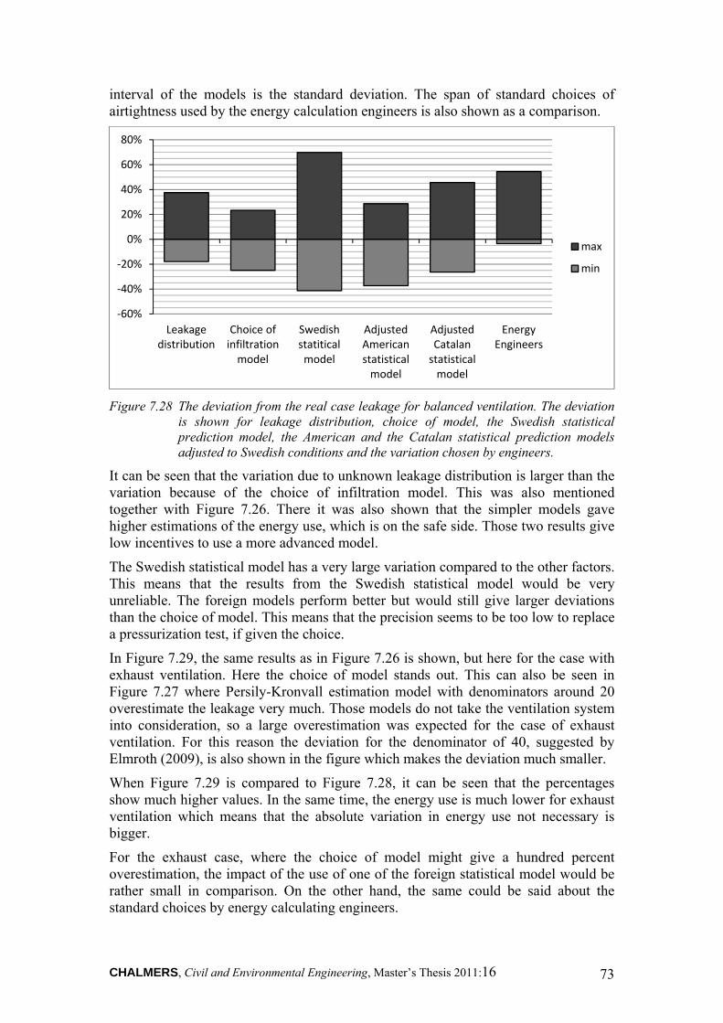
CHALMERS, Civil and Environmental Engineering, Master’s Thesis 2011:16 73
interval of the models is the standard deviation. The span of standard choices of airtightness used by the energy calculation engineers is also shown as a comparison.
Figure 7.28 The deviation from the real case leakage for balanced ventilation. The deviation
is shown for leakage distribution, choice of model, the Swedish statistical prediction model, the American and the Catalan statistical prediction models adjusted to Swedish conditions and the variation chosen by engineers.
It can be seen that the variation due to unknown leakage distribution is larger than the variation because of the choice of infiltration model. This was also mentioned together with Figure 7.26. There it was also shown that the simpler models gave higher estimations of the energy use, which is on the safe side. Those two results give low incentives to use a more advanced model.
The Swedish statistical model has a very large variation compared to the other factors. This means that the results from the Swedish statistical model would be very unreliable. The foreign models perform better but would still give larger deviations than the choice of model. This means that the precision seems to be too low to replace a pressurization test, if given the choice.
In Figure 7.29, the same results as in Figure 7.26 is shown, but here for the case with exhaust ventilation. Here the choice of model stands out. This can also be seen in Figure 7.27 where Persily-Kronvall estimation model with denominators around 20 overestimate the leakage very much. Those models do not take the ventilation system into consideration, so a large overestimation was expected for the case of exhaust ventilation. For this reason the deviation for the denominator of 40, suggested by Elmroth (2009), is also shown in the figure which makes the deviation much smaller.
When Figure 7.29 is compared to Figure 7.28, it can be seen that the percentages show much higher values. In the same time, the energy use is much lower for exhaust ventilation which means that the absolute variation in energy use not necessary is bigger.
For the exhaust case, where the choice of model might give a hundred percent overestimation, the impact of the use of one of the foreign statistical model would be rather small in comparison. On the other hand, the same could be said about the standard choices by energy calculating engineers.
‐60%
‐40%
‐20%
0%
20%
40%
60%
80%
Leakagedistribution
Choice ofinfiltrationmodel
Swedishstatiticalmodel
AdjustedAmericanstatisticalmodel
AdjustedCatalanstatisticalmodel
EnergyEngineers
max
min
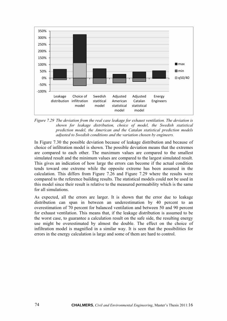
CHALMERS, Civil and Environmental Engineering, Master’s Thesis 2011:16 74
Figure 7.29 The deviation from the real case leakage for exhaust ventilation. The deviation is
shown for leakage distribution, choice of model, the Swedish statistical prediction model, the American and the Catalan statistical prediction models adjusted to Swedish conditions and the variation chosen by engineers.
In Figure 7.30 the possible deviation because of leakage distribution and because of choice of infiltration model is shown. The possible deviation means that the extremes are compared to each other. The maximum values are compared to the smallest simulated result and the minimum values are compared to the largest simulated result. This gives an indication of how large the errors can become if the actual condition tends toward one extreme while the opposite extreme has been assumed in the calculation. This differs from Figure 7.26 and Figure 7.29 where the results were compared to the reference building results. The statistical models could not be used in this model since their result is relative to the measured permeability which is the same for all simulations.
As expected, all the errors are larger. It is shown that the error due to leakage distribution can span in between an underestimation by 40 percent to an overestimation of 70 percent for balanced ventilation and between 50 and 90 percent for exhaust ventilation. This means that, if the leakage distribution is assumed to be the worst case, to guarantee a calculation result on the safe side, the resulting energy use might be overestimated by almost the double. The effect on the choice of infiltration model is magnified in a similar way. It is seen that the possibilities for errors in the energy calculation is large and some of them are hard to control.
‐100%
‐50%
0%
50%
100%
150%
200%
250%
300%
350%
Leakagedistribution
Choice ofinfiltrationmodel
Swedishstatiticalmodel
AdjustedAmericanstatisticalmodel
AdjustedCatalanstatisticalmodel
EnergyEngineers
max
min
q50/40
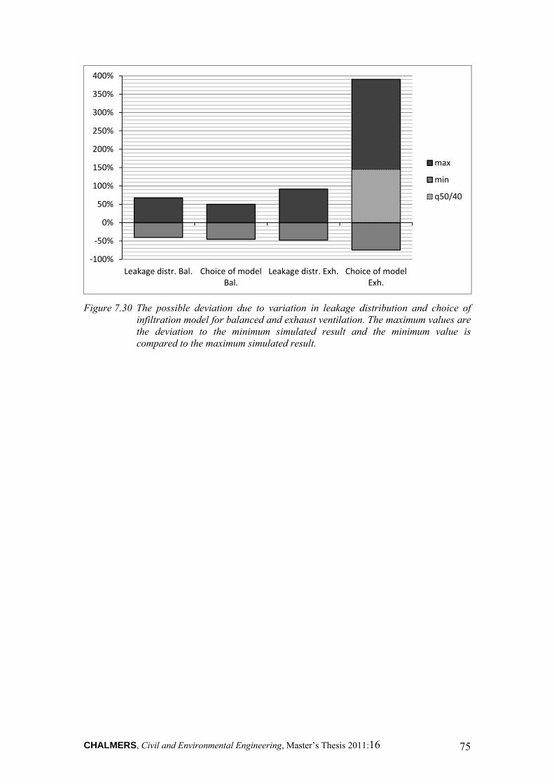
CHALMERS, Civil and Environmental Engineering, Master’s Thesis 2011:16 75
Figure 7.30 The possible deviation due to variation in leakage distribution and choice of
infiltration model for balanced and exhaust ventilation. The maximum values are the deviation to the minimum simulated result and the minimum value is compared to the maximum simulated result.
‐100%
‐50%
0%
50%
100%
150%
200%
250%
300%
350%
400%
Leakage distr. Bal. Choice of modelBal.
Leakage distr. Exh. Choice of modelExh.
max
min
q50/40
CHALMERS, Civil and Environmental Engineering, Master’s Thesis 2011:16 76
8 Conclusions From a review of different studies a number of factors influencing the airtightness were found. One of the most influencing factors for a good airtightness was if the building had been part in an energy efficiency program. This factor is not a specific measure but rather a collection of measures, thus the actual reason for the better airtightness has to be found somewhere else. In a similar way, to have a distinct focus on airtightness during the whole project improves the final result. This could come from worked out measures, as thought through sealing solutions, but also from an increased accuracy in the detail work.
For construction methods, the one measure which gives the largest improvement on the airtightness was to put an installation layer in the wall. To have a heavy wall material and a slab on ground also seems to be superior to light walls and crawlspace or basement. Another important aspect for the airtightness is the building complexity. More floors and especially floors with varying floor area, was found to create larger leakage.
According to the engineers questioned in this thesis, most new projects have a requirement on airtightness today. This value is often used for energy calculations for new buildings; at least before pressurization tests have been performed. For this case, a statistical model would probably perform worse, but a statistical model might here be used by the client to find a reasonable choice of requirement. For buildings without requirements a statistical model could possibly replace experience and give a better estimation for inexperienced engineers.
A direct use of foreign statistical models does not seem to be possible. The results were very far from the measured values. The foreign models tested were from USA and Catalonia. It might look different for a statistical model produced in a closer country, where the climate and the building tradition are more similar to Swedish conditions.
When the models were adjusted with a regression to a Swedish database, the foreign models gave much better prediction. This can be because the reference building was chosen to have a normal airtightness. Thus a random building would have a larger risk of a worse prediction since the standard deviations from the regression line were big.
A more detailed regression, with a larger database would have to be made to see if it is possible to get a better correlation. Although the true correlation between the chosen characteristics evaluated in the model will follow through and become an upper limit of the correlation for the adjusted regression.
The Swedish statistical model had larger deviations than the foreign models. For some of the factors, very few buildings had been used to calculate the averages, which then lead to very large standard deviations. Those deviations would probably be lower if more buildings were used to create the model, but this is not certain since there is an actual spread in the population. More buildings would nevertheless give a better estimate of the true average.
The choice of infiltration model was compared to the possible deviation due to lack of information about the leakage distribution. The leakage distribution creates such a large variation in the resulting energy use, which makes pressurization test results hard to use when aiming for good precision.

CHALMERS, Civil and Environmental Engineering, Master’s Thesis 2011:16 77
For balanced ventilation, the difference between the infiltration models where of the same magnitude as the difference in energy usage due to the distribution of the leakages. All models underestimated the energy usage for the worst case of leakage distribution but the model which gave the largest energy usage and thus was closest to the worst case was Persily-Kronvall estimation model with a denominator of 20 which was the simplest possible model.
For exhaust ventilation the results were more separated. The two more advanced models underestimated the energy usage independent of the leakage distribution while the two simpler models all overestimated the energy usage. So the simpler models would be a safer guess even though the more advanced models were closer to the leakage distribution based on the leakage search.
This leads to the conclusion that for energy calculations, to be on the safe side, which would be to overestimate the effect of the infiltration, there is no reason to use any of the more advanced models. For the climate conditions in Göteborg, the use of a denominator of 20 for balanced ventilation and the denominator of 40 for exhaust ventilation works well.
CHALMERS, Civil and Environmental Engineering, Master’s Thesis 2011:16 78
9 Recommendations for further studies The conclusions in this report are mostly general. It creates an image of areas where knowledge is missing. To handle these unknowns, some further studies could be done:
The report shows a large possible impact from unknown leakage distribution. It would be interesting to see how the actual leakage distribution varies for existing buildings, to see if the span of possible distributions can be limited.
In this report the simplest infiltration calculation models, using q50/20 for balanced ventilation and q50/40 for exhaust ventilation, were the ones that gave the best results while they still were on the safe side. To examine this relation further, the model would have to be tested against different climate conditions and different values for the permeability, q50.
In the report some foreign statistical airtightness prediction models are analyzed. Both models showed weak correlation to Swedish buildings with measured airtightness. To examine the possible use of foreign statistical models they would have to be controlled against a larger database of Swedish buildings. First to find if there is an actual stronger correlation between the used influencing factors and airtightness in Swedish buildings and secondly, if there is a stronger correlation, to get a better regression line to adjust the foreign model to Swedish conditions.
The Swedish model used in the report had worse deviations than the foreign models. This was partly due to the lack of data used for some of the calculated averages. For some factors, buildings with basement and buildings with concrete walls, the average was based on as few as one building. The model could be developed further by analyzing a larger database. Also, the method to choose the weighting factors can be improved.
To open up possibilities to create better statistical models, a standardized system for collecting detailed information during pressurization test would be of interest. The development of such a system would need studies in which factors that influence the airtightness.
CHALMERS, Civil and Environmental Engineering, Master’s Thesis 2011:16 79
10 References AIVC (1996) A Guide to Energy Efficient Ventilation, Air Infiltration and Ventilation
Centre, Coventry, Great Britain, 254 pp. ISBN 0 946075 85 9.
ASHRAE (2009) 2009 ASHRAE handbook – fundamentals. SI edition, American Society of Heating, Refrigeration and Air-Conditioning Engineers, Atlanta, GA. ISBN 1615831703.
ASHRAE (2010) ASHRAE Handbook, Additions and corrections. SI edition [electronic], American Society of Heating, Refrigeration and Air-Conditioning Engineers, Atlanta, GA. Accessible: http://www.ashrae.org > publications > Handbook > General Handbook Corrections - SI Edition [2011-04-07]
Bankvall, C. (1987) Air Movements and the Thermal Performance of the Building Envelope, ASTM American Society for Testing and Materials, Thermal Insulation: Materials and Systems, ASTM STP 922, F.J. Powell and S.L. Matthews, Eds.
Boverket (1993) Boverkets byggregler 1994 (The Swedish building code 1994). 1st edition, Boverket, Stockholm. ISBN 91-7147-130-8.
Boverket (2008) Regelsamling för byggande, BBR 17, Avsnitt 9, energihushållning (Building regulations, BBR 17, Section 9, energy management), Boverket, Karlskrona, pp. 197-205. ISBN 978-91-86045-03-6.
Eliasson, E. (2010) Att uppnå god lufttäthet. (To achieve good air-tightness). Diploma thesis, Department of Civil and Environmental Engineering, Division of Building Technology, Chalmers University of Technology, Göteborg, Sweden, 77 pp.
Elmroth, A. (2009). Byggvägledning 8. Energihushållning och värmeisolering: En handbok i anslutning till Boverkets byggregler. 2nd edition. AB Svensk Byggtjänst, Stockholm, 135 pp. ISBN 978-91-7333-338-2
EN 13829:2000, Thermal performance of buildings- Determination of air permeability of buildings- Fan pressurization method, European standard, European Committee for Standardization, CEN
Etheridge, D. & Sandberg, M.(1996) Building ventilation: theory and measurement 1st edition. John Wiley & Sons, Chichester, New York, 754 pp. ISBN 0 471 96087 X.
Etheridge, D. (1998) A note on crack flow equations for ventilation modelling. Building and Environment. Vol. 33, No 5, 1998, pp. 325-328.
FEBY (2009) Kravspecifikation för passivhus [electronic], Forum för energieffektiva byggnader, Forum för energieffektivt byggande, ATON report 0902, Accessible: http//energieffektivabyggnader.se > rapporter > FEBY_Kravspecifikation_Passiv hus_2009.pdf [2011-04-01]
Hagentoft, C.(2003) Introduction to Building Physics, Studentlitteratur, Lund, 422 pp. ISBN 91-44-01896-7.
Jokisalo, J, Kurnitski, J & Vinha, J (2007) Building leakage, infiltration and energy performance analyses for Finnish detached houses. Proceedings of Clima 2007 WellBeing Indoors, RHEVA World Congress, 10-14 June 2007, Helsinki, Finland.
CHALMERS, Civil and Environmental Engineering, Master’s Thesis 2011:16 80
Jokisalo, J., Kurnitski, J., Korpi, M., Kalamees, T. & Vinha, J. (2009) Building leakage, infiltration, and energy performance analyses for Finnish detached houses, Building and environment. Vol. 44, No 2, 2009, pp.377-387.
Kronvall Johnny (1980) Air flows in building components. Studentlitteratur, Report TVBH-1002, Lund, 194 pp.
Mattsson, B. (2004) Luftläckage i bostäder – litteraturstudier, modellering och mätningar. Licentiate thesis, Department of Civil and Environmental Engineering, Division of Building Technology, Chalmers University of Technology, Göteborg, Sweden, 127 pp.
McWilliams, J. & Jung M. (2006) Development of a Mathematical Air-leakage Model from Measured Data. Lawrence Berkley National Laboratory, Report LBNL-59041, Berkley, CA, 47 pp.
Montoya, M., Pastor, E., Carrié, R.,, Guyot, G. & Planas, E. (2010) Air leakage in Catalan dwellings: Developing an airtightness model and leakage airflow predictions. Building and environment. Vol.45, No. 6, 2010, pp.1458-1469
Petersson, B-Å. (2007) Tillämpad Byggnadsfysik, (Applied Building Physics) 3rd edition, Studentlitteratur, Lund, 524 pp. ISBN978-91-44-04886-4.
Sandberg, P., Sikander, E., Wahlgren, P. & Larsson, B. (2007) Lufttäthetsfrågor I byggprocessen – etapp B. Tekniska konsekvenser och lönsamhetskalkyler. (Consideration of airtightness in the construction process – Stage B. Technical consequences and profitability assessments). SP Sveriges Tekniska Forskningsinstitut, SP Rapport 2007:23, Borås, 58 pp.
Sherman, M. (1987) Estimation of Infiltration from Leakage and Climate Indicators, Energy and Buildings, Vol.10, No 1, 1987, pp.81-86.
Sherman, M. (1998) The Use of Blower-door Data [electronic] Laurence Berkley Laboratory, Report LBL-35173, Berkley; CA, 18 pp. Accessible: http://epb.lbl.gov/publications/lbl-35173.pdf [2011-02-22]
Walker, I., Wilson, D. & Sherman, M. (1997) A comparison of the power law to quadratic formulations for air infiltration calculations. Energy and Buildings. Vol. 27, No. 3, 1997, pp. 293-299.
Walton, G, N & Dols, W, S (2008) CONTAM 2.4c User Guide and program Documentation [electronic], National Institute of Standards and Technology, NISTIR 7251, Gaithersburg, MD, 276 pp. Accessible: www.nist.gov > publications > search: NISTIR 7251 [2011-03-02]
Zou, Y. (2010) Classification of Buildings With Regard to Airtightness, Master’s thesis, Department of Civil and Environmental Engineering, Division of Building Technology, Chalmers University of Technology, Göteborg, Sweden, 82 pp.
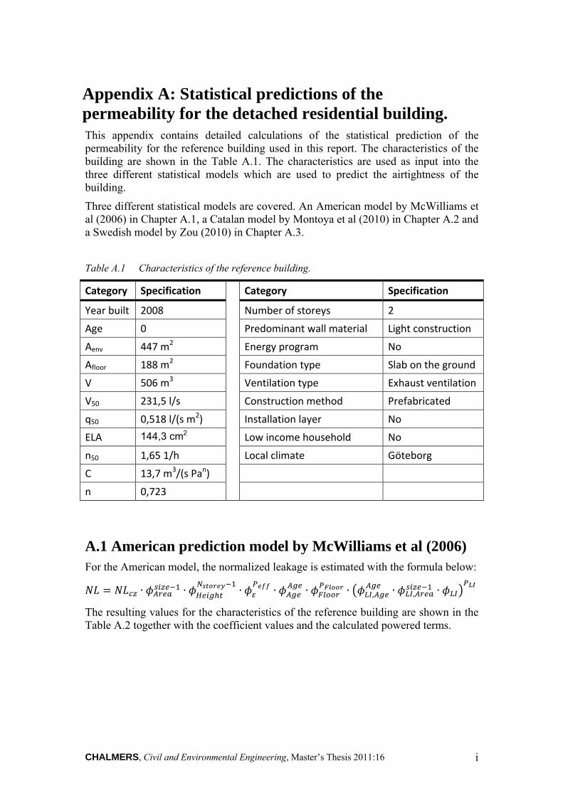
CHALMERS, Civil and Environmental Engineering, Master’s Thesis 2011:16 i
Appendix A: Statistical predictions of the permeability for the detached residential building. This appendix contains detailed calculations of the statistical prediction of the permeability for the reference building used in this report. The characteristics of the building are shown in the Table A.1. The characteristics are used as input into the three different statistical models which are used to predict the airtightness of the building.
Three different statistical models are covered. An American model by McWilliams et al (2006) in Chapter A.1, a Catalan model by Montoya et al (2010) in Chapter A.2 and a Swedish model by Zou (2010) in Chapter A.3.
Table A.1 Characteristics of the reference building.
Category Specification Category Specification
Year built 2008 Number of storeys 2
Age 0 Predominant wall material Light construction
Aenv 447 m2 Energy program No
Afloor 188 m2 Foundation type Slab on the ground
V 506 m3 Ventilation type Exhaust ventilation
V50 231,5 l/s Construction method Prefabricated
q50 0,518 l/(s m2) Installation layer No
ELA 144,3 cm2 Low income household No
n50 1,65 1/h Local climate Göteborg
C 13,7 m3/(s Pan)
n 0,723
A.1 American prediction model by McWilliams et al (2006) For the American model, the normalized leakage is estimated with the formula below:
∙ ∙ ∙ ∙ ∙ ∙ , ∙ , ∙
The resulting values for the characteristics of the reference building are shown in the Table A.2 together with the coefficient values and the calculated powered terms.
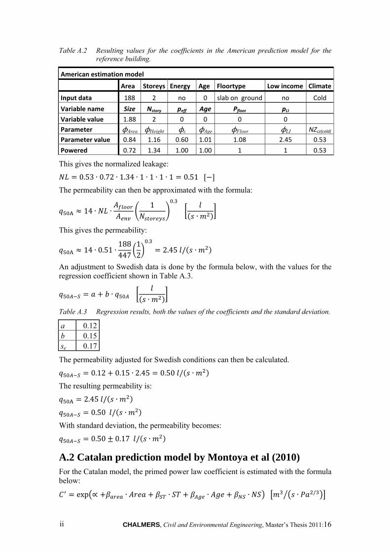
CHALMERS, Civil and Environmental Engineering, Master’s Thesis 2011:16 ii
Table A.2 Resulting values for the coefficients in the American prediction model for the reference building.
American estimation model
Area Storeys Energy Age Floortype Low income Climate
Input data 188 2 no 0 slab on ground no Cold
Variable name Size Nstory peff Age Pfloor pLI
Variable value 1.88 2 0 0 0 0
Parameter ϕArea ϕHeight ϕε ϕAge ϕFloor ϕLI NZcz(cold)
Parameter value 0.84 1.16 0.60 1.01 1.08 2.45 0.53
Powered 0.72 1.34 1.00 1.00 1 1 0.53
This gives the normalized leakage:
0.53 ∙ 0.72 ∙ 1.34 ∙ 1 ∙ 1 ∙ 1 ∙ 1 0.51
The permeability can then be approximated with the formula:
14 ∙ ∙1 .
∙
This gives the permeability:
14 ∙ 0.51 ∙188447
12
.
2.45 / ∙
An adjustment to Swedish data is done by the formula below, with the values for the regression coefficient shown in Table A.3.
∙ ∙
Table A.3 Regression results, both the values of the coefficients and the standard deviation.
a 0.12 b 0.15 se 0.17
The permeability adjusted for Swedish conditions can then be calculated.
0.12 0.15 ∙ 2.45 0.50 / ∙
The resulting permeability is:
2.45 / ∙
0.50 / ∙
With standard deviation, the permeability becomes:
0.50 0.17 / ∙
A.2 Catalan prediction model by Montoya et al (2010) For the Catalan model, the primed power law coefficient is estimated with the formula below:
exp ∝ ∙ ∙ ∙ ∙ ∙ /
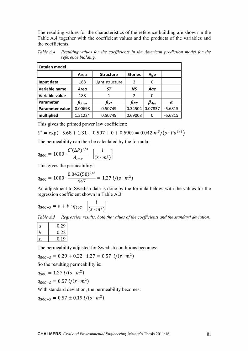
CHALMERS, Civil and Environmental Engineering, Master’s Thesis 2011:16 iii
The resulting values for the characteristics of the reference building are shown in the Table A.4 together with the coefficient values and the products of the variables and the coefficients.
Table A.4 Resulting values for the coefficients in the American prediction model for the reference building.
Catalan model
Area Structure Stories Age
Input data 188 Light structure 2 0
Variable name Area ST NS Age
Variable value 188 1 2 0
Parameter βArea βST βNS βAge αParameter value 0.00698 0.50749 0.34504 0.07837 ‐5.6815
multiplied 1.31224 0.50749 0.69008 0 ‐5.6815
This gives the primed power law coefficient:
exp 5.68 1.31 0.507 0 0.690 0.042 / ∙ /
The permeability can then be calculated by the formula:
1000 ∙′ ∆ /
∙
This gives the permeability:
1000 ∙0.042 50 /
4471.27 / ∙
An adjustment to Swedish data is done by the formula below, with the values for the regression coefficient shown in Table A.3.
∙ ∙
Table A.5 Regression results, both the values of the coefficients and the standard deviation.
a 0.29 b 0.22 se 0.19
The permeability adjusted for Swedish conditions becomes:
0.29 0.22 ∙ 1.27 0.57 / ∙
So the resulting permeability is:
1.27 / ∙
0.57 / ∙
With standard deviation, the permeability becomes:
0.57 0.19 / ∙
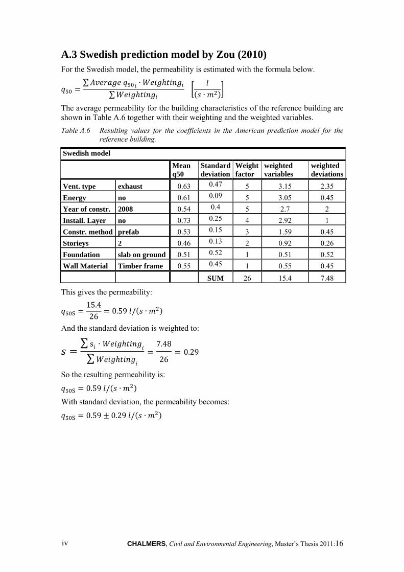
CHALMERS, Civil and Environmental Engineering, Master’s Thesis 2011:16 iv
A.3 Swedish prediction model by Zou (2010) For the Swedish model, the permeability is estimated with the formula below.
∑ ∙∑
∙
The average permeability for the building characteristics of the reference building are shown in Table A.6 together with their weighting and the weighted variables.
Table A.6 Resulting values for the coefficients in the American prediction model for the reference building.
Swedish model
Mean q50
Standard deviation
Weight factor
weighted variables
weighted deviations
Vent. type exhaust 0.63 0.47 5 3.15 2.35
Energy no 0.61 0.09 5 3.05 0.45
Year of constr. 2008 0.54 0.4 5 2.7 2
Install. Layer no 0.73 0.25 4 2.92 1
Constr. method prefab 0.53 0.15 3 1.59 0.45
Storieys 2 0.46 0.13 2 0.92 0.26
Foundation slab on ground 0.51 0.52 1 0.51 0.52
Wall Material Timber frame 0.55 0.45 1 0.55 0.45
SUM 26 15.4 7.48
This gives the permeability:
15.426
0.59 / ∙
And the standard deviation is weighted to:
∑ s ∙
∑7.48
260.29
So the resulting permeability is:
0.59 / ∙ With standard deviation, the permeability becomes:
0.59 0.29 / ∙
CHALMERS, Civil and Environmental Engineering, Master’s Thesis 2011:16 v
Appendix B: Calculation of an example of the leakage distribution. For the leakage distribution 50W80B will 50 percent of the leakages in the plane be toward the windward side and 50 percent is divided among the other sides. Also 80 percent of the leakages are at the bottom of the building in the foundation-wall connection.
This leads to the input data for the leakage distributions as:
0.5
0.8
Where p stands for the part of the leakage at positioned at the section described by the index.
Beneath are the calculations to gain the C coefficient in the power law equation for each leakage. The coefficients are indexed as a combination of the plane and the vertical position. Windward is indexed W and other planar directions are indexed X. Bottom is indexed B and other vertical positions are indexed X. This gives us four different combinations; CWB, CWX, CXB and CXX. Ctot is the C coefficient for the whole envelope which is the sum of the C coefficients of each leakage as long as the exponent n is the same.
The combinations are positioned at a varying amount of places and thus the amount of each type is named; nWB, nWX, nXB and nXX. The amount of each comes from the numerical simulation model which has five position in every of four directions, of which one is positioned at the bottom. Thus there are one positioned at the windward direction at the bottom, three positions at the bottom which are not windward, four of the windward positions which are not at the bottom and the other twelve positions, from a total of twenty, is neither windward nor at the bottom. This gives:
1
4
3
12
With this information, the coefficients can be calculated as:
∙
∙
∙ 1∙
CHALMERS, Civil and Environmental Engineering, Master’s Thesis 2011:16 vi
1 ∙∙
1 ∙ 1∙
As an example, for the reference building in this report, the power law coefficient, Ctot, and the power law exponent, n, is 13.7 m3/(s Pa0.723) and 0.723 respectively. The power law coefficient for the leakages at the bottom of the windward side can then be calculated as:
∙∙
0.5 ∙ 0.81
∙ 13.7 5.48 ∙ .⁄
This gives a function for the flow through those leakages, dependent of the pressure difference over the leakages as:
∆ 5.48 ∆ . ⁄