ANALYSIS OF METHODS FOR FINGER VEIN RECOGNITION A THESIS …

ANALYSIS OF METHODS FOR FINGER VEIN RECOGNITION

A THESIS SUBMITTED TO

THE GRADUATE SCHOOL OF INFORMATICS INSTITUTE

OF

MIDDLE EAST TECHNICAL UNIVERSITY

FARIBA YOUSEFI

IN PARTIAL FULFILLMENT OF THE REQUIREMENTS

FOR

THE DEGREE OF MASTER OF SCIENCE

IN

MEDICAL INFORMATICS

NOVEMBER 2013

Approval of the thesis:


submitted by FARIBA YOUSEFI in partial fulfillment of the requirements for the degree of Masterof Science in Medical Informatics Department, Middle East Technical University by,

Prof. Dr. Nazife Baykal

Dean, Graduate School of Informatics Institute

Assist. Prof. Dr. Yesim Aydın Son

Head of Department, Medical Informatics

Assist. Prof. Dr. Sinan Kalkan

Supervisor, Computer Engineering Dept., METU

Assoc. Prof. Dr. Alptekin Temizel

Co-supervisor, Work Based Learning Studies Dept., METU

Examining Committee Members:

Prof. Dr. Ünal Erkan Mumcuoglu

Medical Informatics Dept., METU

Assist. Prof. Dr. Sinan Kalkan

Computer Engineering Dept., METU

Assoc. Prof. Dr. Alptekin Temizel

Work Based Learning Studies Dept., METU

Assist. Prof. Dr. Aybar Can Acar

Medical Informatics Dept., METU

Assist. Prof. Dr. Banu Günel

Information Systems Dept., METU

Date: 13.11.2013

I hereby declare that all information in this document has been obtained and presented in ac-cordance with academic rules and ethical conduct. I also declare that, as required by these rulesand conduct, I have fully cited and referenced all material and results that are not original tothis work.

Name, Last Name: FARIBA YOUSEFI

Signature :

iii

ABSTRACT


Yousefi, Fariba

M.S., Department of Medical Informatics

Supervisor : Assist. Prof. Dr. Sinan Kalkan

Co-Supervisor : Assoc. Prof. Dr. Alptekin Temizel

November 2013, 103 pages

A decade ago, it was observed that every person has unique finger-vein patterns and that this could be

used for biometric identification. This observation has led to successful identification systems, which

are currently used in banks, hospitals, state organizations, etc. For the feature extraction step of the

finger-vein recognition, which is the most important step, popular methods such as Line Tracking (LT),

Maximum Curvature (MC) and Wide Line Detector (WL) are used in the literature. Among these, the

LT method is very slow in the feature extraction phase. Moreover, LT, MC and WL methods are

susceptible to rotation, translation and noise. To overcome these drawbacks, this thesis proposes us-

ing some popular feature descriptors widely-used in Computer Vision or Pattern Recognition (CVPR)

methods. The CVPR descriptors tested include, Fourier descriptors (FD), Zernike moments (ZM), Lo-

cal Binary Patterns (LBP), Global Binary Patterns (GBP) and Histogram of Oriented Gradients (HOG)

which have not been applied to the finger-vein recognition problem before. The thesis compares these

descriptors against LT, MC and WL and analyze their running time, performance and resilience against

rotation, translation and noise.

Keywords: Finger-vein recognition, Fourier Descriptors, Zernike Moments, Local Binary Patterns,

Histogram of Oriented Gradients

iv

ÖZ

PARMAK DAMAR YAPISI TANIMA METODLARININ ANALIZI

Yousefi, Fariba

Yüksek Lisans, Tıp Bilisimi Bölümü

Tez Yöneticisi : Yrd. Doç. Dr. Sinan Kalkan

Ortak Tez Yöneticisi : Doç. Dr. Alptekin Temizel

Kasım 2013 , 103 sayfa

On yıl önce, her insanın benzersiz parmak damar yapısı oldugu ve bunun biyometrik kimlik için kul-

lanılabilecegi gözlemlenmistir. Bu gözlem, su anda bankalarda, hastanelerde ve devlet kurumlarında

kullanılan basarılı tanımlama sistemlerine öncülük etmistir. Daha önceki çalısmalarda, önemli bir adım

olan parmak damar algılama probleminin öznitelik çıkarma adımı için Çizgi Takibi (LT), Maksimum

Egrilik (MC), Genis Çizgi Bulucu (WL) gibi popüler yollar kullanılmaktadır. LT metodu bunlar ara-

sında öznitelik çıkarma asamasında en yavas olanıdır. Buna ek olarak, LT, MC ve WL metodları ise

döndürülme, tasıma ve gürültü gibi etkenlerden kolay etkilenirler. Bu tez, bahsedilen eksikliklerin üs-

tesinden gelmek için bilgisayarlı görü veya örüntü tanıma (CVPR) metodlarında çokça kullanılan bazı

popüler öznitelik betimleyicileri kullanmayı önermektedir. Bu CVPR betimliyicilerinden Fourier Ta-

nımlayıcıları (FD), Zernike Momentleri (ZM), Yerel Ikili Örüntüler (LBP), Küresel Ikili Örüntüler

(GBP) ve daha önce parmak damar algılama problemine uygulanmamıs olan Yönelimli Bayır Histog-

ramı (HOG) test edilmistir. Bu tez, tüm bu bahsedilen betimleyicileri LT, MC, ve WL ile kıyaslamıstır

ve çalısma zamanlarını, performanslarını ve döndürülme, tasıma ve gürültüye olan dayanıklılıklarını

analiz etmistir.

Anahtar Kelimeler: Parmak-damar tanıma, Fourier Tanımlayıcıları, Zernike Momentleri, Yerel ikili

Örüntüler, Yönelimli Bayır Histogramı

v

To my life

vi

ACKNOWLEDGMENTS

I would like to express my sincere gratitude to my supervisor Assist. Prof. Dr. Sinan Kalkan for the

support, patience, motivation and assistance through the learning process of this master’s thesis.

I would also like to thank my co-supervisor Assoc. Prof. Dr. Alptekin Temizel for his help and advice

through my study.

I am very thankful to KOVAN lab members especially Güner, Sertaç and Hande for their helps. Güner

without you my Turkish would be perfect! Once again thank for all your help.

I would like to express my gratitude towards my family for their best wishes and support especially

my mother.

My sincere thanks go to my fiance for his patience, being with me in good and bad times, and being

supportive.

My special thanks go to my friends whom were always there for me during my hard times especially

Yousef, Negin, Mona and Pardis.

Finally, I would like to thank my loved ones, who have cared about me throughout entire process, and

were patient enough to listen to me. I will be grateful forever for your love.

vii

TABLE OF CONTENTS

ABSTRACT . . . . . . . . . . . . . . . . . . . . . . . . . . . . . . . . . . . . . . . . . . . . . iv

ÖZ . . . . . . . . . . . . . . . . . . . . . . . . . . . . . . . . . . . . . . . . . . . . . . . . . . v

ACKNOWLEDGMENTS . . . . . . . . . . . . . . . . . . . . . . . . . . . . . . . . . . . . . . vii

TABLE OF CONTENTS . . . . . . . . . . . . . . . . . . . . . . . . . . . . . . . . . . . . . . viii

LIST OF TABLES . . . . . . . . . . . . . . . . . . . . . . . . . . . . . . . . . . . . . . . . . xii

LIST OF FIGURES . . . . . . . . . . . . . . . . . . . . . . . . . . . . . . . . . . . . . . . . . xiii

LIST OF ABBREVIATIONS . . . . . . . . . . . . . . . . . . . . . . . . . . . . . . . . . . . . xxii

CHAPTERS

1 INTRODUCTION . . . . . . . . . . . . . . . . . . . . . . . . . . . . . . . . . . . . 1

1.1 Identification and Authentication Process . . . . . . . . . . . . . . . . . . . . 1

1.2 Motivation, Scope and Contributions of the Thesis . . . . . . . . . . . . . . . 2

1.3 Outline of the Thesis . . . . . . . . . . . . . . . . . . . . . . . . . . . . . . . 2

2 BIOMETRICS . . . . . . . . . . . . . . . . . . . . . . . . . . . . . . . . . . . . . . 3

2.1 Some Advantages and Disadvantages of Biometrics . . . . . . . . . . . . . . 3

2.2 Biometric Characteristics . . . . . . . . . . . . . . . . . . . . . . . . . . . . 4

2.3 Biometric System Architecture . . . . . . . . . . . . . . . . . . . . . . . . . 5

2.4 Biometric Types . . . . . . . . . . . . . . . . . . . . . . . . . . . . . . . . . 6

viii

2.4.1 Facial Scan . . . . . . . . . . . . . . . . . . . . . . . . . . . . . . 6

2.4.2 Iris Scan . . . . . . . . . . . . . . . . . . . . . . . . . . . . . . . . 6

2.4.3 Voice Scan . . . . . . . . . . . . . . . . . . . . . . . . . . . . . . 6

2.4.4 Fingerprint Recognition . . . . . . . . . . . . . . . . . . . . . . . 7

2.4.5 Finger-Vein Recognition . . . . . . . . . . . . . . . . . . . . . . . 7

2.4.5.1 Devices for Finger-vein Image Acquisition . . . . . . . 7

2.4.5.2 Some advantages and disadvantages of Finger-Vein Sys-

tems . . . . . . . . . . . . . . . . . . . . . . . . . . . 8

2.5 Evaluation of Biometric Authentication Systems . . . . . . . . . . . . . . . . 9

2.5.1 False Acceptance Rate and False Rejection Rate . . . . . . . . . . . 9

2.5.2 Equal Error Rate . . . . . . . . . . . . . . . . . . . . . . . . . . . 9

2.5.3 Receiver Operating Characteristic Curve . . . . . . . . . . . . . . . 10

3 FINGER-VEIN RECOGNITION METHODS . . . . . . . . . . . . . . . . . . . . . . 11

3.1 Finger Vein Recognition Algorithms Analyzed in this Study . . . . . . . . . . 11

3.1.1 Line Tracking . . . . . . . . . . . . . . . . . . . . . . . . . . . . . 12

3.1.2 Maximum Curvature . . . . . . . . . . . . . . . . . . . . . . . . . 15

3.1.3 Wide Line Detector . . . . . . . . . . . . . . . . . . . . . . . . . . 16

3.1.4 Shape Descriptors . . . . . . . . . . . . . . . . . . . . . . . . . . . 18

3.1.5 Fourier Descriptors . . . . . . . . . . . . . . . . . . . . . . . . . . 18

3.1.6 Image Moments . . . . . . . . . . . . . . . . . . . . . . . . . . . . 19

3.1.6.1 Zernike Moments . . . . . . . . . . . . . . . . . . . . 20

3.1.7 Local Binary Patterns . . . . . . . . . . . . . . . . . . . . . . . . . 22

ix

3.1.8 Histogram of Oriented Gradients . . . . . . . . . . . . . . . . . . . 24

3.1.9 Global Binary Patterns . . . . . . . . . . . . . . . . . . . . . . . . 24

3.2 Finger Vein Matching . . . . . . . . . . . . . . . . . . . . . . . . . . . . . . 26

3.2.1 Template Matching . . . . . . . . . . . . . . . . . . . . . . . . . . 28

3.2.2 Euclidean Distance . . . . . . . . . . . . . . . . . . . . . . . . . . 28

3.2.3 Chi-Square Distance (χ2) . . . . . . . . . . . . . . . . . . . . . . . 28

3.2.4 Earth Mover’s Distance (EMD) . . . . . . . . . . . . . . . . . . . 29

4 EXPERIMENTS . . . . . . . . . . . . . . . . . . . . . . . . . . . . . . . . . . . . . 31

4.1 The Database . . . . . . . . . . . . . . . . . . . . . . . . . . . . . . . . . . 31

4.2 Performance Measurement . . . . . . . . . . . . . . . . . . . . . . . . . . . 33

4.3 Results . . . . . . . . . . . . . . . . . . . . . . . . . . . . . . . . . . . . . . 33

4.3.1 Line Tracking . . . . . . . . . . . . . . . . . . . . . . . . . . . . . 34

4.3.2 Maximum Curvature . . . . . . . . . . . . . . . . . . . . . . . . . 34

4.3.3 Wide Line Detector . . . . . . . . . . . . . . . . . . . . . . . . . . 34

4.3.4 Fourier Descriptors . . . . . . . . . . . . . . . . . . . . . . . . . . 36

4.3.5 Zernike Moments . . . . . . . . . . . . . . . . . . . . . . . . . . . 36

4.3.6 Local Binary Patterns . . . . . . . . . . . . . . . . . . . . . . . . . 36

4.3.7 Histogram of Oriented Gradients . . . . . . . . . . . . . . . . . . . 38

4.3.8 GBP . . . . . . . . . . . . . . . . . . . . . . . . . . . . . . . . . . 38

4.4 Comparison of Performances . . . . . . . . . . . . . . . . . . . . . . . . . . 38

4.5 Comparison of Running Times . . . . . . . . . . . . . . . . . . . . . . . . . 40

4.6 Discussion . . . . . . . . . . . . . . . . . . . . . . . . . . . . . . . . . . . . 40

x

4.6.1 Evaluation of the results with respect to the literature . . . . . . . . 45

5 CONCLUSION . . . . . . . . . . . . . . . . . . . . . . . . . . . . . . . . . . . . . . 49

5.1 Future Work . . . . . . . . . . . . . . . . . . . . . . . . . . . . . . . . . . . 49

REFERENCES . . . . . . . . . . . . . . . . . . . . . . . . . . . . . . . . . . . . . . . . . . . 51

APPENDICES

A DETAILED RESULTS ON THE PERFORMANCE OF THE METHODS . . . . . . . 55

xi

LIST OF TABLES

Table 4.1 Running-time comparison of all methods. . . . . . . . . . . . . . . . . . . . . . . . 46

Table 4.2 Comparison of resilience to rotation, translation and noise . . . . . . . . . . . . . . . 46

Table 4.3 Comparison to the reported results in the finger-vein recognition literature. . . . . . . 47

xii

LIST OF FIGURES

Figure 2.1 Enrollement to a biometric system: First, the biometric data is captured. Then,

extracted information is stored in an enrollment template and the template is stored in the

database (adapted from [10]). . . . . . . . . . . . . . . . . . . . . . . . . . . . . . . . . . 3

Figure 2.2 Authentication with a biometric system: First, the biometric data is captured. Then,

extracted information is stored in an enrollment template and the template is compared to

the one in the database (adapted from [10]). . . . . . . . . . . . . . . . . . . . . . . . . . . 4

Figure 2.3 Biometric System (adapted from [1]). . . . . . . . . . . . . . . . . . . . . . . . . . 5

Figure 2.4 Vascular network captured using infrared light (Source: [1]). . . . . . . . . . . . . . 8

Figure 2.5 (a) A finger-vein image capturing device, (b) a sample captured image (Source: [2]). 8

Figure 2.6 Sample ROC Curves. . . . . . . . . . . . . . . . . . . . . . . . . . . . . . . . . . . 10

Figure 3.1 Cross-sectional brightness profile of a vein. (a) Cross-sectional profile, (b) Position

of cross-sectional profile (Source: [2]). . . . . . . . . . . . . . . . . . . . . . . . . . . . . 12

Figure 3.2 Dark line detection; this example shows spatial relationship between the current

tracking point (xc, yc) and the cross-sectional profile. Pixel p is the neighboring pixel of the

current tracking point and the cross-sectional s − p − t looks like a valley. As a result the

current tracking point is on a dark line (Source: [2]). . . . . . . . . . . . . . . . . . . . . . 14

Figure 3.3 (a) An example infrared image, (b) Locus space table extracted using the Line Track-

ing method (Source: [2]). . . . . . . . . . . . . . . . . . . . . . . . . . . . . . . . . . . . 14

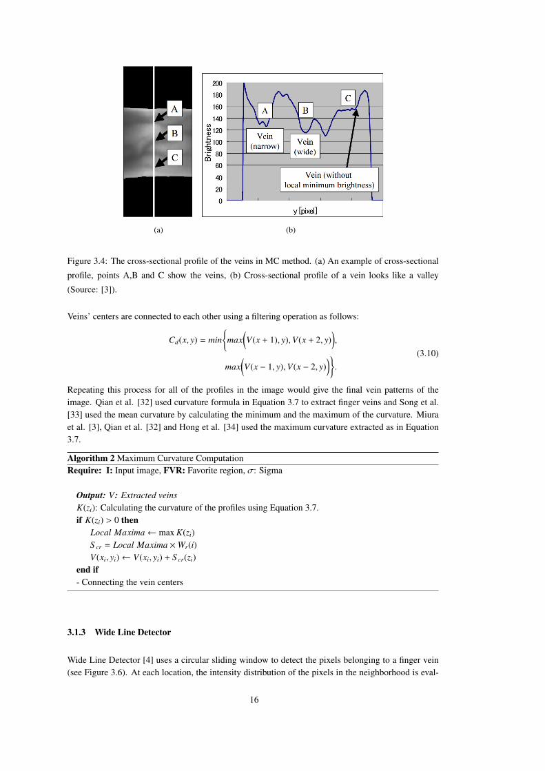
Figure 3.4 The cross-sectional profile of the veins in MC method. (a) An example of cross-

sectional profile, points A,B and C show the veins, (b) Cross-sectional profile of a vein

looks like a valley (Source: [3]). . . . . . . . . . . . . . . . . . . . . . . . . . . . . . . . . 16

xiii

Figure 3.5 Relationship among the profile, the curvature and the probability score of the veins

(Source: [3]). . . . . . . . . . . . . . . . . . . . . . . . . . . . . . . . . . . . . . . . . . . 17

Figure 3.6 The circular neighborhood region (Source: [4]). . . . . . . . . . . . . . . . . . . . 17

Figure 3.7 Mapping transform (Source: [39]). . . . . . . . . . . . . . . . . . . . . . . . . . . 21

Figure 3.8 Zernike radial polynomials of order 0-5 (Source: [39]). . . . . . . . . . . . . . . . . 21

Figure 3.9 Local Binary Patterns computation. The extracted value from the center pixel is:

1+2+4+8+128=143 (Source: [43]) . . . . . . . . . . . . . . . . . . . . . . . . . . . . . . 23

Figure 3.10 Best Bit Map computation (adapted from [25]). . . . . . . . . . . . . . . . . . . . . 24

Figure 3.11 Local Line Binary Patterns computation (Source: [45]). . . . . . . . . . . . . . . . 25

Figure 3.12 Histogram of Oriented Gradients computation (Source: [47]). . . . . . . . . . . . . 26

Figure 3.13 GBP computation. (a) The binary image; (b) Rows are multiplied by powers of two;

(c) Each row is summed horizontally; (d) Columns are multiplied by powers of two; (e)

Columns are summed vertically; (f) Resulting GBP descriptor (Source: [9]). . . . . . . . . 27

Figure 3.14 Ilustration of GBP along an arbitrary direction with orientation θ (Source: [9]). . . . 27

Figure 4.1 Example finger-vein images by (a-e) Rotation (0o, 5o, 10o, 15o, 20o degrees, respec-

tively) , (f-j) Translation (0, 5, 10, 15, 20 pixels, respectively), (k-o) Gaussian noise (0.0002, 0.0004, 0.0006, 0.0008, 0.001

variances, respectively). As can be seen in noisy images, increasing the Gaussian noise de-

grades the visibility of the veins. . . . . . . . . . . . . . . . . . . . . . . . . . . . . . . . 32

Figure 4.2 Sample of Images from the SDUMLA-HMT Finger-vein Database . . . . . . . . . 33

Figure 4.3 Finding the mask for the finger region in the image. (a) Original image, (b) Prewitt

edge detection, (c) Masked image. . . . . . . . . . . . . . . . . . . . . . . . . . . . . . . 33

Figure 4.4 Example finger-vein extraction by the LT method. (a) Masked image, (b) Image

extracted from locus table, (c) Binarized version of (b) using median thresholding. . . . . . 34

Figure 4.5 FAR vs. FRR graph for LT based on (a) Rotation, (b) Translation, (c) Gaussian noise. 35

xiv

Figure 4.6 Example finger-vein extraction by the MC method. (a) Masked image, (b) Binary

image produced by the MC method. . . . . . . . . . . . . . . . . . . . . . . . . . . . . . . 36

Figure 4.7 FAR vs. FRR graph for MC based on (a) Rotation, (b) Translation, (c) Gaussian noise. 37

Figure 4.8 Example finger-vein extraction by the WL method. (a) Masked image, (b) Binary

image produced by the WL method. . . . . . . . . . . . . . . . . . . . . . . . . . . . . . . 38

Figure 4.9 FAR vs. FRR graph for WL based on (a) Rotation, (b) Translation, (c) Gaussian noise. 39

Figure 4.10 Analysis of distance and rotation (a) Euclidean, (b) χ2, (c) EMD. . . . . . . . . . . 41

Figure 4.11 Analysis of distance and translation (a) Euclidean, (b) χ2, (c) EMD. . . . . . . . . . 42

Figure 4.12 Analysis of distance and Gaussian noise (a) Euclidean, (b) χ2, (c) EMD. . . . . . . 43

Figure 4.13 FAR vs. FRR graphs for the best of all methods compared with LT+mismatch,

MC+mismatch and WL+mismatch (a) Using Euclidean distance, (b) Using χ2 distance,

(c) Using Earth Mover’s distance. . . . . . . . . . . . . . . . . . . . . . . . . . . . . . . . 44

Figure 4.14 Best of Euclidean, χ2 and Earth Mover’s distances . . . . . . . . . . . . . . . . . . 45

Figure A.1 FAR vs. FRR graph for FD-LT variations using Euclidean distance matching based

on (a) Rotation, (b) Translation, (c) Gaussian noise. . . . . . . . . . . . . . . . . . . . . . 56

Figure A.2 FAR vs. FRR graph for FD-LT variations using χ2 distance matching based on (a)

Rotation, (b) Translation, (c) Gaussian noise. . . . . . . . . . . . . . . . . . . . . . . . . . 57

Figure A.3 FAR vs. FRR graph for FD-LT variations using Earth Mover’s distance matching

based on (a) Rotation, (b) Translation, (c) Gaussian noise. . . . . . . . . . . . . . . . . . . 58

Figure A.4 FAR vs. FRR graph for FD-MC variations using Euclidean distance matching based


Figure A.5 FAR vs. FRR graph for FD-MC variations using χ2 distance matching based on (a)


Figure A.6 FAR vs. FRR graph for FD-MC variations using Earth Mover’s distance matching


xv

Figure A.7 FAR vs. FRR graph for FD-WL variations using Euclidean distance matching based


Figure A.8 FAR vs. FRR graph for FD-WL variations using χ2 distance matching based on (a)


Figure A.9 FAR vs. FRR graph for FD-WL variations using Earth Mover’s distance matching


Figure A.10FAR vs. FRR graph for ZM-LT variations using Euclidean distance matching based


Figure A.11FAR vs. FRR graph for ZM-LT variations using χ2 distance matching based on (a)


Figure A.12FAR vs. FRR graph for ZM-LT variations using Earth Mover’s distance matching


Figure A.13FAR vs. FRR graph for ZM-MC variations using Euclidean distance matching based


Figure A.14FAR vs. FRR graph for ZM-MC variations using χ2 distance matching based on (a)


Figure A.15FAR vs. FRR graph for ZM-MC variations using Earth Mover’s distance matching


Figure A.16FAR vs. FRR graph for ZM-WL variations using Euclidean distance matching based


Figure A.17FAR vs. FRR graph for ZM-WL variations using χ2 distance matching based on (a)


Figure A.18FAR vs. FRR graph for ZM-WL variations using Earth Mover’s distance matching


Figure A.19FAR vs. FRR graph for LBP-LT variations using Euclidean distance matching based


xvi

Figure A.20FAR vs. FRR graph for LBP-LT variations using χ2 distance matching based on (a)


Figure A.21FAR vs. FRR graph for LBP-LT variations using Earth Mover’s distance matching


Figure A.22FAR vs. FRR graph for LBP-MC variations using Euclidean distance matching


Figure A.23FAR vs. FRR graph for LBP-MC variations using χ2 distance matching based on

(a) Rotation, (b) Translation, (c) Gaussian noise. . . . . . . . . . . . . . . . . . . . . . . . 78

Figure A.24FAR vs. FRR graph for LBP-MC variations using Earth Mover’s distance matching


Figure A.25FAR vs. FRR graph for LBP-WL variations using Euclidean distance matching


Figure A.26FAR vs. FRR graph for LBP-WL variations using χ2 distance matching based on


Figure A.27FAR vs. FRR graph for LBP-WL variations using Earth Mover’s distance matching


Figure A.28FAR vs. FRR graph for HOG-LT variations using Euclidean distance matching


Figure A.29FAR vs. FRR graph for HOG-LT variations using χ2 distance matching based on


Figure A.30FAR vs. FRR graph for HOG-LT variations using Earth Mover’s distance matching


Figure A.31FAR vs. FRR graph for HOG-MC variations using Euclidean distance matching


Figure A.32FAR vs. FRR graph for HOG-MC variations using χ2 distance matching based on


xvii

Figure A.33FAR vs. FRR graph for HOG-MC variations using Earth Mover’s distance matching


Figure A.34FAR vs. FRR graph for HOG-WL variations using Euclidean distance matching


Figure A.35FAR vs. FRR graph for HOG-WL variations using χ2 distance matching based on


Figure A.36FAR vs. FRR graph for HOG-WL variations using Earth Mover’s distance matching


Figure A.37FAR vs. FRR graph for GBP-LT variations using Euclidean distance matching based


Figure A.38FAR vs. FRR graph for GBP-LT variations using χ2 distance matching based on (a)


Figure A.39FAR vs. FRR graph for GBP-LT variations using Earth Mover’s distance matching


Figure A.40FAR vs. FRR graph for GBP-MC variations using Euclidean distance matching


Figure A.41FAR vs. FRR graph for GBP-MC variations using χ2 distance matching based on


Figure A.42FAR vs. FRR graph for GBP-MC variations using Earth Mover’s distance matching


Figure A.43FAR vs. FRR graph for GBP-WL variations using Euclidean distance matching


Figure A.44FAR vs. FRR graph for GBP-WL variations using χ2 distance matching based on


Figure A.45FAR vs. FRR graph for GBP-WL variations using Earth Mover’s distance matching


xviii

Figure A.46FAR vs. FRR graphs for all methods using Euclidean distance (a) FD on LT, MC

and WL. (b) ZM on LT, MC, WL. (c) HOG on LT, MC and WL. (d) GBP on LT, MC and

WL. (e) LBP on LT, MC and WL. . . . . . . . . . . . . . . . . . . . . . . . . . . . . . . . 101

Figure A.47FAR vs. FRR graphs for all methods using χ2 distance (a) FD on LT, MC and WL.

(b) ZM on LT, MC, WL. (c) HOG on LT, MC and WL. (d) GBP on LT, MC and WL. (e)

LBP on LT, MC and WL. . . . . . . . . . . . . . . . . . . . . . . . . . . . . . . . . . . . 102

Figure A.48FAR vs. FRR graphs for all methods using Earth Mover’s distance (a) FD on LT,

MC and WL. (b) ZM on LT, MC, WL. (c) HOG on LT, MC and WL. (d) GBP on LT, MC

and WL. (e) LBP on LT, MC and WL. . . . . . . . . . . . . . . . . . . . . . . . . . . . . 103

xix

xx

List of Algorithms

1 Line Tracking Computation . . . . . . . . . . . . . . . . . . . . . . . . . . . . . . . . 15

2 Maximum Curvature Computation . . . . . . . . . . . . . . . . . . . . . . . . . . . . 16

3 Wide Line Detector Computation . . . . . . . . . . . . . . . . . . . . . . . . . . . . . 18

4 Fourier descriptors Computation . . . . . . . . . . . . . . . . . . . . . . . . . . . . . 19

5 Zernike Moments Computation . . . . . . . . . . . . . . . . . . . . . . . . . . . . . . 22

6 Local Binary Patterns Computation (adapted from [9]) . . . . . . . . . . . . . . . . . 23

7 Histograms of Oriented Gradients Computation (adapted from [9]) . . . . . . . . . . . 25

8 Global Binary Patterns (GBPh) Computation (adapted from [9]). . . . . . . . . . . . . 26

xxi

LIST OF ABBREVIATIONS

χ2 Chi-Square distance

LT Line Tracking

MC Maximum Curvature

WL Wide Line Detector

FD Fourier Descriptors

ZM Zernike Moments

FV Finger Vein

FP Finger Print

FG Finger Geometry

Id Identifier

HP Hewlett-Packard

Fvr Favorite

img Image

LBP Local Binary Patterns

GBP Global Binary Patterns

HOG Histogram of Oriented Gradients

LDP Local Derivative Patterns

CGF Circular Gabor Filter

FAR False Acceptance Rate

FRR False Rejection Rate

EER Equal Error Rate

ROC Receiver Operating Characteristic

PCA Principle Component Analysis

PIN Personal Identification Number

EMD Earth Mover’s Distance

CVPR Computer Vision and Pattern Recognition

xxii

xxiv

CHAPTER 1

INTRODUCTION

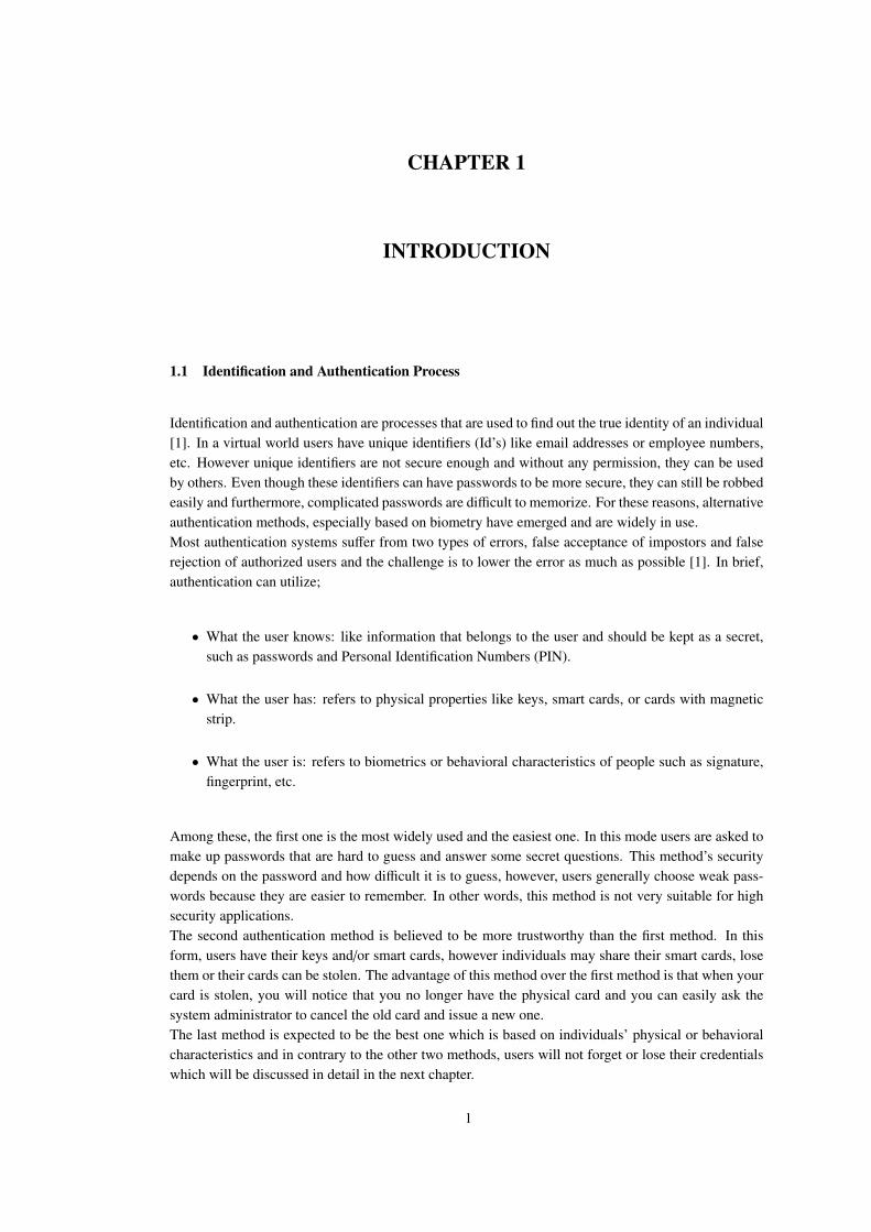
1.1 Identification and Authentication Process

Identification and authentication are processes that are used to find out the true identity of an individual[1]. In a virtual world users have unique identifiers (Id’s) like email addresses or employee numbers,etc. However unique identifiers are not secure enough and without any permission, they can be usedby others. Even though these identifiers can have passwords to be more secure, they can still be robbedeasily and furthermore, complicated passwords are difficult to memorize. For these reasons, alternativeauthentication methods, especially based on biometry have emerged and are widely in use.Most authentication systems suffer from two types of errors, false acceptance of impostors and falserejection of authorized users and the challenge is to lower the error as much as possible [1]. In brief,authentication can utilize;

• What the user knows: like information that belongs to the user and should be kept as a secret,such as passwords and Personal Identification Numbers (PIN).

• What the user has: refers to physical properties like keys, smart cards, or cards with magneticstrip.

• What the user is: refers to biometrics or behavioral characteristics of people such as signature,fingerprint, etc.

Among these, the first one is the most widely used and the easiest one. In this mode users are asked tomake up passwords that are hard to guess and answer some secret questions. This method’s securitydepends on the password and how difficult it is to guess, however, users generally choose weak pass-words because they are easier to remember. In other words, this method is not very suitable for highsecurity applications.The second authentication method is believed to be more trustworthy than the first method. In thisform, users have their keys and/or smart cards, however individuals may share their smart cards, losethem or their cards can be stolen. The advantage of this method over the first method is that when yourcard is stolen, you will notice that you no longer have the physical card and you can easily ask thesystem administrator to cancel the old card and issue a new one.The last method is expected to be the best one which is based on individuals’ physical or behavioralcharacteristics and in contrary to the other two methods, users will not forget or lose their credentialswhich will be discussed in detail in the next chapter.

1

There are many biometric technology types such as fingerprint1, finger vein, facial scan, iris scanand voice scan, each of which has their own advantages and disadvantages. However there is no bestmethod among them, depending on the requirements of the application and people that would use thesesystems, the preferences would be different.

1.2 Motivation, Scope and Contributions of the Thesis

Finger vein recognition is one of the forefront methods in biometric technology in recent years. Manysuccessful methods such as Line Tracking (LT) [2], Maximum Curvature (MC) [3] and Wide LineDetector (WL) [4] have been proposed for finger vein recognition. Among these methods, LT has avery slow matching and feature extraction phase. Moreover, LT, MC and WL are rotation dependent,and they are affected by image noise. To overcome these drawbacks, using some popular featuredescriptors widely used for several Computer Vision or Pattern Recognition (CVPR) are proposed.These descriptors include Fourier Descriptors (FD) [5], Zernike Moments (ZM) [6], Histogram ofOriented Gradients (HOG) [7], Local Binary Patterns (LBP) [8] and Global Binary Patterns (GBP)[9]. Among these, FD, ZM, HOG, LBP and GBP have not been applied to the finger vein recognitionbefore. These descriptors are compared against LT, MC and WL. The novelty of the thesis is in (i)applying new feature extraction methods that have not been used for finger vein recognition beforeand (ii) evaluating the performance of all these methods under translation, rotation and noise. Thefocus is on the “feature extraction” step, and the preprocessing step is kept as simple as possible. Asfor matching, the matching method specific to LT, MC and WL which is called mismatch ratio is usedand for all other descriptors, three different distance metrics called Euclidean distance, χ2 (Chi-Squaredistance) and Earth Mover’s Distance (EMD) have been applied and compared to each other. Forperformance evaluation, the SDUMLA-HMT finger vein database that is publicly available2 is used.The contributions of the thesis have been accepted for “the 9th International Joint Conference onComputer Vision, Imaging and Computer Graphics Theory and Applications, VISAPP”3.

1.3 Outline of the Thesis

The rest of the thesis is organized as follows. Chapter 2 describes background information aboutbiometrics and different biometric systems’ advantages and disadvantages. Chapter 3 describes featureextraction methods that has been applied to the finger vein in this thesis like LT, MC, WL, FD, ZM,HOG, LBP and GBP and different matching methods such as Euclidean distance, χ2 and EMD areanalyzed. Moreover, some state of the art studies are discussed in this chapter. Chapter 4 comparesthe performance of the mentioned methods under rotation, translation and noise, then their runningtimes and accuracies are evaluated and compared against the results in the literature. Finally chapter5 concludes the thesis with a summary of the contributions and an outlook for how the work can beimproved further as future work.

1 The word “finger vein” is written separately unlike “fingerprint”. See: http://www.merriam-webster.com/dictionary/fingerprint

2 http://mla.sdu.edu.cn/sdumla-hmt.html3 http://www.visapp.visigrapp.org/

2

CHAPTER 2

BIOMETRICS

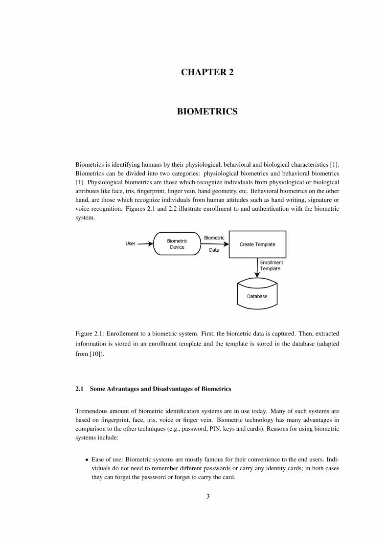
Biometrics is identifying humans by their physiological, behavioral and biological characteristics [1].Biometrics can be divided into two categories: physiological biometrics and behavioral biometrics[1]. Physiological biometrics are those which recognize individuals from physiological or biologicalattributes like face, iris, fingerprint, finger vein, hand geometry, etc. Behavioral biometrics on the otherhand, are those which recognize individuals from human attitudes such as hand writing, signature orvoice recognition. Figures 2.1 and 2.2 illustrate enrollment to and authentication with the biometricsystem.

BiometricDevice

Database

Create TemplateBiometric

Data

Enrollment Template

User

Figure 2.1: Enrollement to a biometric system: First, the biometric data is captured. Then, extracted

information is stored in an enrollment template and the template is stored in the database (adapted

from [10]).

2.1 Some Advantages and Disadvantages of Biometrics

Tremendous amount of biometric identification systems are in use today. Many of such systems arebased on fingerprint, face, iris, voice or finger vein. Biometric technology has many advantages incomparison to the other techniques (e.g., password, PIN, keys and cards). Reasons for using biometricsystems include:

• Ease of use: Biometric systems are mostly famous for their convenience to the end users. Indi-viduals do not need to remember different passwords or carry any identity cards; in both casesthey can forget the password or forget to carry the card.

3

BiometricDevice

Compare TemplatesDatabase

Create TemplateBiometric

Data

Enrollment

Template

Match Template

User

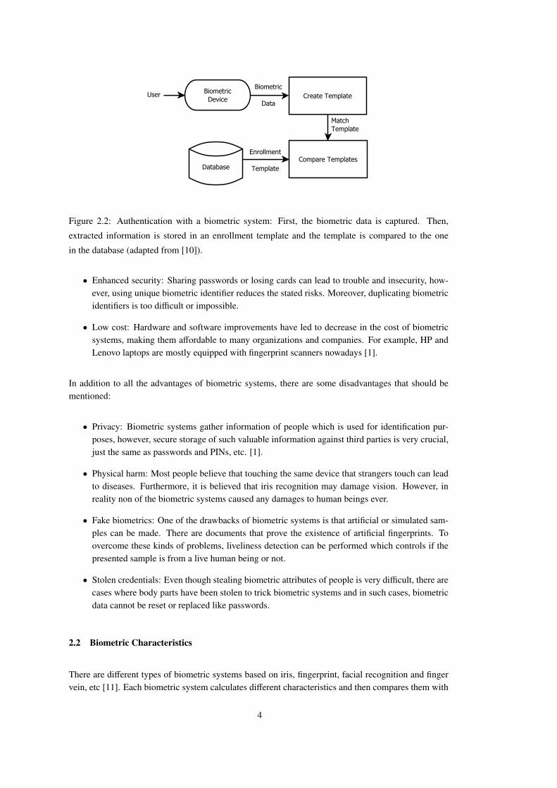
Figure 2.2: Authentication with a biometric system: First, the biometric data is captured. Then,

extracted information is stored in an enrollment template and the template is compared to the one

in the database (adapted from [10]).

• Enhanced security: Sharing passwords or losing cards can lead to trouble and insecurity, how-ever, using unique biometric identifier reduces the stated risks. Moreover, duplicating biometricidentifiers is too difficult or impossible.

• Low cost: Hardware and software improvements have led to decrease in the cost of biometricsystems, making them affordable to many organizations and companies. For example, HP andLenovo laptops are mostly equipped with fingerprint scanners nowadays [1].

In addition to all the advantages of biometric systems, there are some disadvantages that should bementioned:

• Privacy: Biometric systems gather information of people which is used for identification pur-poses, however, secure storage of such valuable information against third parties is very crucial,just the same as passwords and PINs, etc. [1].

• Physical harm: Most people believe that touching the same device that strangers touch can leadto diseases. Furthermore, it is believed that iris recognition may damage vision. However, inreality non of the biometric systems caused any damages to human beings ever.

• Fake biometrics: One of the drawbacks of biometric systems is that artificial or simulated sam-ples can be made. There are documents that prove the existence of artificial fingerprints. Toovercome these kinds of problems, liveliness detection can be performed which controls if thepresented sample is from a live human being or not.

• Stolen credentials: Even though stealing biometric attributes of people is very difficult, there arecases where body parts have been stolen to trick biometric systems and in such cases, biometricdata cannot be reset or replaced like passwords.

2.2 Biometric Characteristics

There are different types of biometric systems based on iris, fingerprint, facial recognition and fingervein, etc [11]. Each biometric system calculates different characteristics and then compares them with

4

its database to check if the individual should be given access to the system or not. There are varioustypes of biometric characteristics, however, some important types are:

• Uniqueness: Each person has unique biological characteristics that makes him/her different fromothers. These particular biometrics can be divided into three groups, called genetics, phenotypicand behavioural [11].

– Genetics: Features like hair and eye color that the user has inherited from his/her parent.

– Phenotypic: Certain biometric features like iris patterns, fingerprint patterns and vein net-work.

– Behavioural: Features such as signature or voice can be categorized into this group.

• Performance: Measures how much time and equipment is needed for calculating the matchingprocess. Some techniques are cheaper and faster, like fingerprint or finger vein. On the otherhand, some techniques are costly and slow, like DNA based biometric systems.

• Accuracy: Measures how accurate the system is working, e.g. how many people are by mistakerejected while others are falsely accepted.

• Acceptability: Acceptability shows if the users are comfortable using the biometric systems ornot, for example not many people are comfortable using retina recognition.

2.3 Biometric System Architecture

Four main components of each biometric system are obtaining data, processing, making decision andstorage [11] (see Figure 2.3):

Capture(Data Acquisition)

Process(Signal Processing) Storage

Compare(Decision Policy)

Capture(Data Acquisition)

Process(Signal Processing)

No Match

Match

Enrollment:

PresentBiometrics

PresentBiometrics

Verification:

Figure 2.3: Biometric System (adapted from [1]).

• Data acquisition: In this step the biometric data is captured digitally and then sent to the signalprocessing step.

• Signal processing: Raw data is received in this step and the preprocessing and/or feature extrac-tion methods are performed.

5

• Decesion policy: Final decision would be made in this step to see if the enrollment should beaccepted or rejected.

• Storage: In this step, biometric template is stored for future matching.

2.4 Biometric Types

As mentioned before, there are different types of biometrics, and humans can be recognized by theirfingers, hands, face, eyes, and voice, some of which are more widely used than others. In this sectioneach technique will be discussed briefly and its advantages and disadvantages will be mentioned.

2.4.1 Facial Scan

Facial scan technology is mostly used for identification of individuals instead of verification1. Thistechnology uses some of the important features of the face, like, eyes, nose, lips, and so on [12]. Oneof the advantages of facial scan technology is identifying individuals from distance, therefore, it willnot annoy people by touching any device. Moreover, images can be captured by different devices likevideo cameras. On the other hand, this technology has some disadvantages. For example, the qualityof the captured image is dependent on lightening, background and angle of the camera. Moreover,users’ appearance can change over time, and having glasses, beard, mustache, make-up or differenthair styles, would have an impact on accuracy. Furthermore, having higher accuracy requires savingdifferent images of users which in turn requires more memory space.

2.4.2 Iris Scan

Iris scan technology is used for both identification and verification based on unique features of irises.This technology uses patterns that form the visual part of the iris to differentiate between humans [12].Some advantages are that (i) this system has smallest False Acceptance Rate (FAR) among the otherbiometric systems, which is critical for high secure applications and (ii) iris does not change in timelike some other biometric types (like voice that can change). However, positioning of the head andeye are very important to get accurate results and people should not move their heads during dataacquisition. Iris is a very small area, therefore, captured image should be very high resolution whichmakes the device expensive. Individuals feel discomfortable using this device even though they do notknow infrared scan is used during the process [13].

2.4.3 Voice Scan

Various vocal qualities such as frequency, short-time spectrum of dialogue and spectograms (time-frequency-energy patterns) are used for voice scan [12]. The devices e.g. microphones used for thistechnology are quite cheap. This system lets the users select an expression and repeat it during identifi-cation and verification which reduces the risk of impostors guessing the same phrase and entering intothe system. However noise and echoes can reduce the system accuracy. Moreover voice can change

1 The word “identification” has different meaning than “verification”. See http://www.merriam-webster.com/dictionary/identification and http://www.merriam-webster.com/dictionary/verification

6

during illness or in different moods, making authentication problematic. Enrollment to the voice-basedsystem is longer than other biometric systems because users have to repeat the phrase for many times.

2.4.4 Fingerprint Recognition

Fingerprints are the inherent part of humans and they are unique for each person. Even twins havedifferent fingerprints [14]. Using the patterns found on the finger tips, fingerprint biometric data iscaptured. As with every technology, using fingerprint for biometrics has its own advantages and dis-advantages. Age of the user, dryness and wetness of the finger, temporary or permanent cuts on thefinger, or dirt on the fingerprint scanner all cause the fingerprints to have weak patterns of ridge andvalleys that can degrade the performance of a fingerprint biometric system. The mentioned issues leadto poor recognition rates in fingerprint identification system and users would experience difficultieswith the system’s authentication process. Furthermore, as discussed before there can be artificial fin-gers which threaten system’s security. For creating artificial fingers a copy of the real fingerprint isrequired which can be obtained when the victim is touching objects like glasses and can be replicatedin gelatin. For making the systems secure against artificial fingers, liveliness detection can be used.Liveliness detection searches for certain attributes which can only be found on the live fingers such asthe pulse in the fingertip, however, individuals have different heart rate which can be different fromtime to time and for detecting the fingertip pulse, users need to keep their fingers on the sensor withoutmoving for few seconds. However, there are artificial fingers called wafer thin artificial fingers, thatcan fool such a system by producing pulse.

2.4.5 Finger-Vein Recognition

Disadvantages of fingerprint technology made scientists to think about using what is underneath theskin. Under the skin there are blood vessels which are unique to individuals (even in twins) [1] andthis uniqueness made a new biometric system based on finger veins. Biometrics based on veins, i.e.,vascular biometrics are not limited to the fingers. Retina, face and hands can be identified usingvascular properties too, however, the hardware devices used for finger vein identification are morepreferred than the others because people are used to using their fingers for identification already. Forcapturing a vascular network, hemoglobin plays an important role by absorbing infrared light, andafter absorbing infrared light vein patterns are captured (see Figure 2.4).

Distance is very important in absorbing infrared light between skin and vessels: bigger distance leadsto more noise in the captured image. Palms, back of the hands and fingers can be used as biometricdata, however, people mostly prefer to use their fingers.

2.4.5.1 Devices for Finger-vein Image Acquisition

Finger-vein biometric systems use infrared (IR) light to capture blood vessels, however, the position ofinfrared light source affects the quality of the images. Moreover, the image acquisition device shouldbe small and cheap, and it should provide high resolution images. In captured images, the veins appearas gray patterns. As can be seen in Figure 2.5 finger is placed between the Infrared Light EmittingDiodes (IR-LEDs) and imaging device.

7

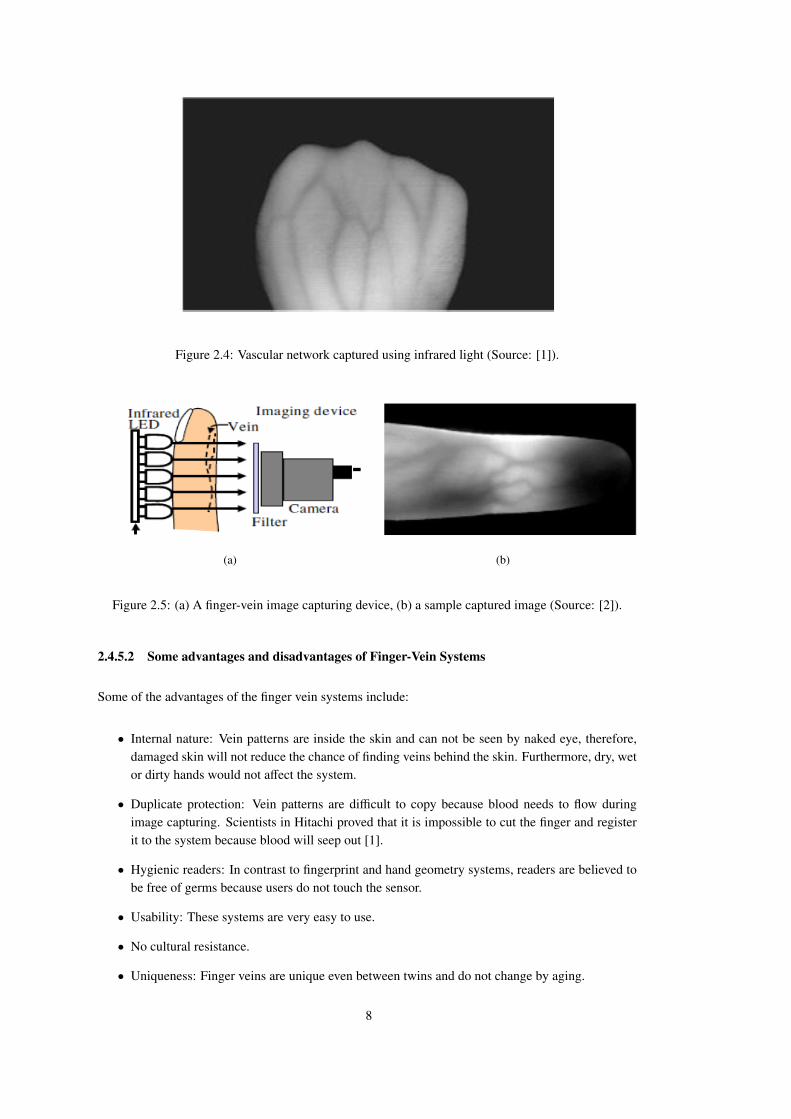
Figure 2.4: Vascular network captured using infrared light (Source: [1]).

(a) (b)

Figure 2.5: (a) A finger-vein image capturing device, (b) a sample captured image (Source: [2]).

2.4.5.2 Some advantages and disadvantages of Finger-Vein Systems

Some of the advantages of the finger vein systems include:

• Internal nature: Vein patterns are inside the skin and can not be seen by naked eye, therefore,damaged skin will not reduce the chance of finding veins behind the skin. Furthermore, dry, wetor dirty hands would not affect the system.

• Duplicate protection: Vein patterns are difficult to copy because blood needs to flow duringimage capturing. Scientists in Hitachi proved that it is impossible to cut the finger and registerit to the system because blood will seep out [1].

• Hygienic readers: In contrast to fingerprint and hand geometry systems, readers are believed tobe free of germs because users do not touch the sensor.

• Usability: These systems are very easy to use.

• No cultural resistance.

• Uniqueness: Finger veins are unique even between twins and do not change by aging.

8

• Fast processing: There are algorithms that can be processed very fast by the system.

• Harmless: No one reported any side effect of using finger veins’ systems on human health.

• Reliability: This system provides trustworthy results that can be used in high secure applications.

Some of the disadvantages of the finger-vein systems include:

• Light controlling: Lights can affect the system, however, for external uses there are covers tosolve this problem.

• Alignment: There are finger guidance for putting the finger correctly inside the reader becausemisalignment would capture wrong patterns.

2.5 Evaluation of Biometric Authentication Systems

Important metrics and methods used in the evaluation of biometric systems are discussed in this sec-tion. These are False Acceptance Rate (FAR), False Rejection Rate (FRR), Equal Error Rate (EER)and Receiver Operating Characteristic (ROC) curve [10].

2.5.1 False Acceptance Rate and False Rejection Rate

Biometric systems evaluate a matching score to recognize if the person that tries to enter into thesystem is a genuine user or an impostor. Selecting the proper threshold (twenty threshold values areused in this study and different threshold values are calculated by dividing the difference between themaximum and minimum of the distances by twenty) is important for matching, though, if the thresholdis too low, genuine users will be rejected and if the threshold is too high then impostors would enterthe system. Therefore, depending on the security requirements, the threshold should be set properlybetween them. FAR and FRR metrics are defined as follows:

FAR =number of succesful authentications by impostors

number of attemps at authentication by unauthorized users. (2.1)

FRR =number of failed attemps at authentication by authorized users

number of attemps at authentication by genuine users. (2.2)

Both FAR and FRR are dependent on the threshold; by increasing the threshold, one will be decreasedand the other will be increased and vice versa.

2.5.2 Equal Error Rate

As mentioned before, by decreasing the threshold more authorized users will be rejected, and at thesame time less unauthorized users will be accepted. At some point, FAR and FRR become equal. Thevalue of FAR and FRR at that point is called the Equal Error Rate. EER does not give any informationabout the values of FAR and FRR at different thresholds, however, can be used to compare differentbiometric systems.

9

0 0.2 0.4 0.6 0.8 10

0.2

0.4

0.6

0.8

1

FAR

FR

R

LTMCWL

Figure 2.6: Sample ROC Curves.

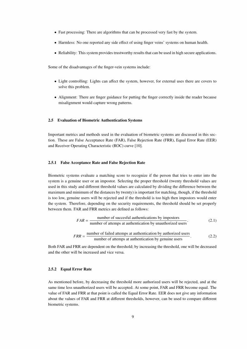
2.5.3 Receiver Operating Characteristic Curve

A Receiver operating characteristic (ROC) curve displays FAR versus FRR. False accepted impostorsrate is shown on the x axis of the curve and false rejected genuine rate is displayed on the y axis ofthe curve. A ROC curve is useful for summing up the performance of biometric systems. Figure 2.6shows sample ROC curves.FAR and FRR are functions of a threshold T , and can be shown as follows:

ROC(T ) = (FAR(T ), FRR(T ))→

(0, 1) as T → 0

(1, 0) as T → ∞.(2.3)

As can be seen in Equation 2.3, FAR and FRR are opposite of each other, as one of them increases, theother one decreases.

10

CHAPTER 3

FINGER-VEIN RECOGNITION METHODS

As discussed in Chapter 2, biometric human identification has become very important due to pitfallseven in extreme security systems, and alternative methods that can be used in place of or together withfingerprint have been being sought during the last decade. It has been shown that finger vein patternis distinctive enough for human biometric identification [15] and with the advent of technology, andespecially since finger vein is more difficult to manipulate compared to, e.g., fingerprints, many suc-cessful applications have been seen.Existing studies regarding finger vein feature extraction can be divided into three main categories(without aiming to be comprehensive):

i) Those that use filtering or transforming methods: Such methods mainly use Gabor filters toextract filter responses using the Gabor function at different scales and/or orientations [16], [17],[18] and [19]. Steerable filters [20] and wavelets [21] are used the same as Gabor filter for imageenhancement or feature extraction. After filtering, from the filter responses, using histograms,minimum-maximum or average values, features are extracted, and these features are usuallycompared using Euclidean distance or Cosine distance [17]. Moreover, Fourier transform [22]can be applied to the finger vein images and the phase components of the images can be takenas feature vectors.

ii) Those that track finger veins, segment the pixels corresponding to the veins, and represent ordirectly compare these pixels [2], [23].

iii) Those that use descriptive feature extraction methods such as Local Binary Patterns [24], [25]or Local Derivative Patterns [24]. In the literature Kang et al. [26] used LDP for finger veinrecognition and Mirmohamadsadeghi et al. [27] used LDP for palm vein recognition.

Moreover, there are machine learning methods that can be applied to the finger vein for feature extrac-tion such as neural networks [28] and Principle Component Analysis (PCA) [29].

3.1 Finger Vein Recognition Algorithms Analyzed in this Study

For finger vein extraction, the literature mostly uses methods such as Line Tracking (LT), MaximumCurvature (MC) and Wide Line Detector (WL) and these methods are dependent to translation androtation and sensitive to noise. To overcome these drawbacks, some popular feature descriptors whichare widely used for several computer vision and pattern recognition (CVPR) problems in the literature

11

are used in this thesis. Moreover, various matching methods have been used for matching the featuresextracted from each method. In this study, for LT, MC and WL, the so-called mismatch ratio is usedin which a query map is compared against the stored map pixel by pixel (like in template matching).For FD, ZM, HOG, LBP and GBP, distance metrics like Euclidean distance, χ2 and Earth Mover’sDistance are used.

3.1.1 Line Tracking

The Line Tracking method of Miura et al. [2] [30] is one of the leading approaches used in finger-veinextraction. The method exploits the fact that, due to the light-absorbing nature of the finger veins, theyappear darker in the image, making them look like valleys in the infrared image (see Figure 3.1). TheLT method is based on randomly finding a pixel in a valley and tracking the pixels along the valleyas much as possible. To determine whether a pixel is on a valley (i.e., a part of the finger vein), theLT method checks whether the cross-section s − p − t which is orthogonal to the center pixel, formsa valley in intensity values (see Figure 3.2). The method tracks “valley pixels” and if the pixel is noton a valley, the method restarts randomly in another position in the image for tracking finger-veins.The output is a locus table that lists how many times a pixel has been tracked, and this captures thefinger-vein in the infrared image (see Figure 3.3).

(a) (b)

Figure 3.1: Cross-sectional brightness profile of a vein. (a) Cross-sectional profile, (b) Position of

cross-sectional profile (Source: [2]).

Steps required to compute LT method is given in Algorithm 1 [2] [30]. The details about the algorithmof line tracking are as follows;

Step 1: Selecting the starting point and moving directionThe starting point is selected randomly from the finger vein region and the moving directionattribute (which prevents the tracking point from having excessive curvature) is calculated as

12

follows:

Dlr =

(1, 0) i f (Rnd(2) < 1)

(−1, 0) otherwise.(3.1)

Dud =

(0, 1) i f (Rnd(2) < 1)

(0,−1) otherwise,(3.2)

where Rnd(n) is a random number between 0 and n.

Step 2: Dark-line direction determination and the tracking point movementIn this step, the locus position table will be initialized. This table stores how many times a pixelhas been tracked. To move the tracking point, some limitations should be considered. Theselimitations are described verbally below and defined formally in Equations 3.3 and 3.4:

• The next tracking point should be inside the finger region (R f ).

• The next tracking point should not be the previous tracking point in the current trackinground (Tc).

• Next tracking point should be one of the neighboring pixels as in Equation 3.4.

Nc = Tc ∩ R f ∩ Nr(xc, yc), (3.3)

Nr(xc, yc) =

N3(Dlr(xc, yc)) i f (Rnd(100) < plr)

N3(Dud(xc, yc)) i f (plr + 1 ≤ Rnd(100) < plr + pud)

N8(xc, yc) i f (plr + pud + 1 ≤ Rnd(100)),

(3.4)

where (xc, yc) refer to the current tracking point, N8(x, y) refer to the eight neighboring pixelsof (xc, yc) and N3(D)(x, y) (which is defined as (Dx,Dy)) refer to the three neighboring pixelsof (xc, yc) that is in the direction of moving direction attribute D. Furthermore, D refers to thedirection attribute (see Equations 3.1 and 3.2). N3(D(xc, yc)) is defined as follows:

N3(D)(x, y) =

{(Dx + x,Dy + y),

(Dx − Dy + x,Dy − Dx + y),

(Dx + Dy + x,Dy + Dx + y)}.

(3.5)

plr and pud in Equation 3.4 are the probabilities in which three neighboring pixels can be selectedin the horizontal or vertical direction. Horizontal neighboring pixels will have larger probabilitythan the vertical ones because veins tend to be horizontal. Using Equation 3.6, the depth ofthe valley is calculated and the maximum depth in the cross-sectional profile around the currenttracking point is selected (see Figure 3.2):

Vl = max{

F(xc + r cos θi −

W2

sin θi, yc + r sin θi +W2

cos θi

)+ F

(xc + r cos θi +

W2

sin θi, yc + r sin θi −W2

cos θi

)(3.6)

− 2F (xc + r cos θi, yc + r sin θi)},

where W is the width of the cross-section, r is the distance between the current tracking point(xc, yc) and the cross-section, and θ is the angle between lines (xc, yc)− (xc + 1, yc) and (xc, yc)−(xi, yi).

13

Figure 3.2: Dark line detection; this example shows spatial relationship between the current tracking

point (xc, yc) and the cross-sectional profile. Pixel p is the neighboring pixel of the current tracking

point and the cross-sectional s − p − t looks like a valley. As a result the current tracking point is on a

dark line (Source: [2]).

Step 3: Incrementing the values of the elements in the locus tableIn this step number of times that points in the locus table have been tracked are updated.

Step 4: Repetition: Steps 1 to 3 are repeated for N many iterations, where N is a parameter to the method.

Step 5: Extracting the finger vein patternThe last step is extracting the finger vein pattern that will be obtained from the locus space tableas shown in Figure 3.3.

In the literature, there are many studies based on the Repeated Line Tracking algorithm such as Yanget al. [31] and Qin et al. [23].

(a) (b)

Figure 3.3: (a) An example infrared image, (b) Locus space table extracted using the Line Tracking

method (Source: [2]).

14

Algorithm 1 Line Tracking ComputationRequire: I: Input image, FVR: Favorite region, R: Radius, W: Width of the profiles

Output: V: Extracted veins

- Initialize Locus Table (Tr) to Zeros- StartPoint: Select random points (xs, ys) within FAV region- Randomly select xs ← xs + 1 OR xs ← xs − 1- Randomly select ys ← ys + 1 OR ys ← ys − 1while V > 0 do

- Determine the moving candidate point set Nc

Nc ← Tc ∩ R f ∩ Nr(xc, yc)if size(Nc) = 0 thenV = −1

end iffor i = 1 to size(Nc) do

- Finding the valley (Vl) using Equation 3.6end forindex← arg max

xVl(x)

Tr(yc, xc)← Tr(yc, xc) + 1xc, yc← Nc(index)

end while

3.1.2 Maximum Curvature

Miura et al. [3] proposed a method based on calculating the local maximum curvatures in the cross-sectional profiles of a vein image (see Figure 3.4). In this method, the center positions of the veinsfound using the maximum curvature are extracted and connected to each other to make the final image(Algorithm 2) [3]. The curvature of a profile is calculated using the Equation 3.7.

K(z) =

d2P f (z)dz2{

1 +

(dP f (z)

dz

)2} 32

, (3.7)

where F is a finger image, F(x, y) is the intensity of the pixel (x, y), z is the position in the profile andP f (z) is the cross-section profile.If K(z) is positive, the cross-section profile would be concave, and if K(z) is negative, the cross-sectionprofile would be convex. In each concave area, the local maximums are calculated and these maximapoints show the center positions of the veins. The concave width is considered as well, therefore, usingboth the center position and the width of a concave area, by taking into account scores that are assignedto these center positions as in Equation 3.8:

S cr(zi) = K(zi) ×Wr(i), (3.8)

where i = 0, 1, ...,N − 1 and N is the number of local maximas. Wr(i) is the width of the concaveregions. The output is the plane V, which is created with the assigned scores as in Equation 3.9 (seeFigure 3.5):

V(xi, yi) = V(xi, yi) + S cr(zi). (3.9)

15

(a) (b)

Figure 3.4: The cross-sectional profile of the veins in MC method. (a) An example of cross-sectional

profile, points A,B and C show the veins, (b) Cross-sectional profile of a vein looks like a valley

(Source: [3]).

Veins’ centers are connected to each other using a filtering operation as follows:

Cd(x, y) = min{

max(V(x + 1), y),V(x + 2, y)

),

max(V(x − 1, y),V(x − 2, y)

)}.

(3.10)

Repeating this process for all of the profiles in the image would give the final vein patterns of theimage. Qian et al. [32] used curvature formula in Equation 3.7 to extract finger veins and Song et al.[33] used the mean curvature by calculating the minimum and the maximum of the curvature. Miuraet al. [3], Qian et al. [32] and Hong et al. [34] used the maximum curvature extracted as in Equation3.7.

Algorithm 2 Maximum Curvature ComputationRequire: I: Input image, FVR: Favorite region, σ: Sigma

Output: V: Extracted veinsK(zi): Calculating the curvature of the profiles using Equation 3.7.if K(zi) > 0 then

Local Maxima← max K(zi)S cr = Local Maxima ×Wr(i)V(xi, yi)← V(xi, yi) + S cr(zi)

end if- Connecting the vein centers

3.1.3 Wide Line Detector

Wide Line Detector [4] uses a circular sliding window to detect the pixels belonging to a finger vein(see Figure 3.6). At each location, the intensity distribution of the pixels in the neighborhood is eval-

16

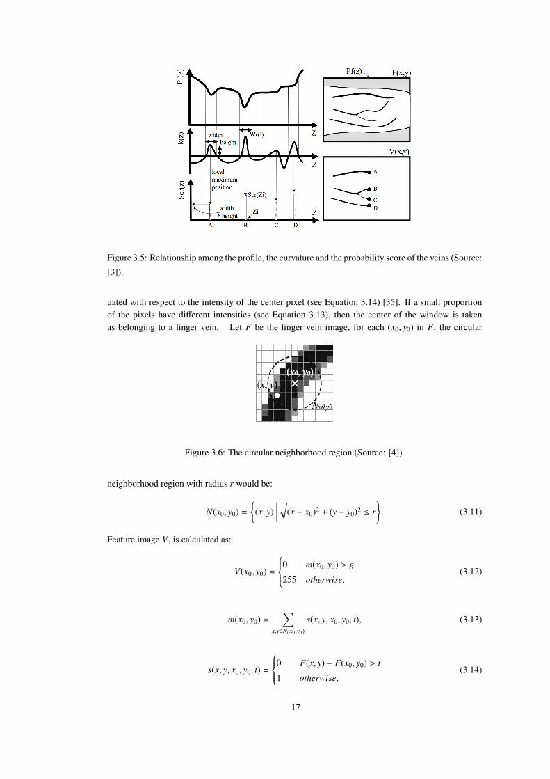
Figure 3.5: Relationship among the profile, the curvature and the probability score of the veins (Source:

[3]).

uated with respect to the intensity of the center pixel (see Equation 3.14) [35]. If a small proportionof the pixels have different intensities (see Equation 3.13), then the center of the window is takenas belonging to a finger vein. Let F be the finger vein image, for each (x0, y0) in F, the circular

Figure 3.6: The circular neighborhood region (Source: [4]).

neighborhood region with radius r would be:

N(x0, y0) =

{(x, y)

∣∣∣∣∣ √(x − x0)2 + (y − y0)2 ≤ r}. (3.11)

Feature image V , is calculated as:

V(x0, y0) =

0 m(x0, y0) > g

255 otherwise,(3.12)

m(x0, y0) =∑

x,y∈N( x0,y0)

s(x, y, x0, y0, t), (3.13)

s(x, y, x0, y0, t) =

0 F(x, y) − F(x0, y0) > t

1 otherwise,(3.14)

17

where V(x0, y0) is the matrix of the finger vein that is calculated using the Equation 3.12, g and t arethe threshold values. Huang et al. assigned g = 41 and t = 1 for the intensity ranges of [0, 255].m calculates sum of the pixels that have different intensities and s groups the pixels that have similarintensities with the one in the center of the mask.

Algorithm 3 Wide Line Detector ComputationRequire: I: Input image, FVR: Favorite Region, r: Radius, t: Threshold, g: Geometric threshold

Output: V: Extracted veins- Creating circular mask:

N ← X2 + Y2 ≤ r2

- Calculating s:F(x, y) − F(x0, y0) ≤ t

- Calculating m:∑x,y∈N( x0,y0) s(x, y, x0, y0, t)

- Apply Equation 3.12- Mask the vein image with the finger region

3.1.4 Shape Descriptors

There are two ways of representing a shape’s region:

• Representing a region by its external characteristics e.g., the boundary.

• Representing a region by its internal characteristics i.e. the pixels that cover the region).

When focus is on a shape’s characteristics, boundary representation is mostly used [5]. On the otherhand, when focus is on the regional properties, internal representation is used [5]. In both cases, thefeatures that are extracted as descriptors should be insensitive to the changes in rotation, translationand scale [5]. Rotation invariance is achieved if the representation of the shape does not changesignificantly by rotation. Translation invariance is achieved if representation of the shape does notchange notably by translation. Fourier descriptors and Zernike moments are discussed in detail in thefollowing sections because in the literature they are good examples of shape descriptors.

3.1.5 Fourier Descriptors

Fourier descriptors are one of the widely used methods for describing shapes [5]. Fourier descriptorsis a contour based descriptor which means that, the pixels on the boundary of the images are used todescribe the shape. The first step to compute Fourier descriptors is to extract the image’s boundarypixels; (x0, y0), (x1, y1), ..., (xN−1, yN−1). These coordinates can be shown in the form of x(k) = xk andy(k) = yk. Therefore, the boundary can be represented as s(k) = [x(k), y(k)], for k = 0, 1, 2, ...,K − 1.Furthermore, these coordinates can be represented as complex numbers s(k) = x(k) + jy(k), wherej =

√−1. The last step is converting s(k) from the spatial domain to the frequency domain using

Discrete Fourier Transform [5] (see Equation3.15).

a(u) =1K

K−1∑k=0

S (k)e− j2πuk

K , (3.15)

18

for u = 0, 1, 2, ...,K − 1. a(u), which are complex, are the Fourier descriptors of the shape’s boundary.FD is normalized using Equation 3.16. Translating the image affects only the first Fourier coefficient,therefore, by removing the first coefficient, FD becomes translation invariant. Rotation invariancecan be achieved by using just the magnitude of the Fourier transform. Moreover, scale invariance isobtained by dividing each coefficient by the first coefficient [36], [37]:

FD =

∣∣∣∣∣FD1

FD0

∣∣∣∣∣, ∣∣∣∣∣FD2

FD0

∣∣∣∣∣, ..., ∣∣∣∣∣ FDk

FD0

∣∣∣∣∣, (3.16)

where k is the number of the coefficients. In short, the steps for computing the Fourier descriptors canbe found in Algorithm 4.

Algorithm 4 Fourier descriptors ComputationRequire: I: Input image, k: Number of coefficients

Output: FD: Fourier coefficientsI = I > 0- Converting coordinates to complex numbers:

I ← I(:, 1) + j ∗ I(:, 2)z← FFT (I)- FD Normalization using Equation 3.16- Take the k first coefficients

3.1.6 Image Moments

Image moments have become one of the popular methods for feature extraction in recent years. Varioustypes of moment descriptors have been used for pattern recognition, registration and compression.When global properties of the image (compared to local properties) are the key points, moments aremostly used. In this section, the geometric moments and the orthogonal moments are explained briefly.In 1962, Hu [38] proposed the first moment invariants for image analysis and pattern recognition.

• Geometric Moments: Two dimensional geometric moment of order (n + m) of a function f(x,y),e.g., the boundary of a shape, is as follows:

Mnm =

∫x

∫y

xnym f (x, y)dxdy. (3.17)

Some properties of the geometric moments are:

– Mass and Area: Zero order moment of the function f (x, y) is:

M00 =

∫x

∫y

f (x, y)dxdy, (3.18)

which shows the total mass of a function or an image and in the case of binary image, M00

represents the total area of the image.

– Center of Mass: The two first order moments, (M10,M01), express the center of the massof the image. Center of the mass is a place where the entire mass of the image can begathered. Coordinates of the center of the mass are:

x =M10

M00, y =

M01

M00. (3.19)

Equation 3.19 can be used to describe the centroid position of the shape.

19

The basis set, xnym, is not orthogonal, though lack of orthogonality in geometric moments,causes information redundancy which means image would not be reconstructed properly usingits geometric moments. On the other hand, these moments are translation and scale invariant,therefore, before using Zernike moments, image preprocessing can be used to achieve translationand scale invariant images.

• Orthogonal Moments: Teague [6] proposed a set of orthogonal moments to overcome geometricmoments’ problems on information loss. There are different types of orthogonal moments. SinceZernike moments is a good representation of orthogonal moments in the literature, it is describedin detail in the following section.

3.1.6.1 Zernike Moments

Zernike moments are shape descriptors which are subcategory of the region-based descriptors [39].As mentioned in Section 3.1.4, region based descriptors use all the pixels inside an area to buildthe descriptors. Zernike moments project an image onto a set of complex Zernike polynomials andthese polynomials are orthogonal to each other. For computing Zernike moments two steps should beconsidered. The first step is calculating the Zernike basis functions and the second step is computingthe Zernike moments by projecting an image to the basis functions [39]. The set of these complexpolynomials called Zernike basis functions are denoted by Vnm(x, y), and defined as follows:

Vnm(x, y) = Vnm(ρ, θ) = Rnm(ρ) exp( jmθ), (3.20)

where n ≥ 0, m > 0 or m < 0 with the conditions of n−|m| being even and |m| ≤ n, ρ is the length of thevector from the origin to (x, y), and θ is the angle between the vector and x axis in counter clockwisedirection. The radial polynomial Rnm(ρ) is defined as follows:

Rnm(ρ) =

n−|m|2∑

s=0

(−1)s.(n − s)!

s!( n+|m|2 − s)!( n−|m|

2 − s)!ρn−2s. (3.21)

Radial polynomials (see Figure 3.8) are orthogonal and satisfy:"x2+y2≤1

[Vnm(x, y)]∗Vpq(x, y)dxdy =π

n + 1δnpδmq, (3.22)

with

δ =

1 a = b

0 otherwise,(3.23)

where V∗ is the complex conjugate of V and δ is the Kronecker delta function. Zernike moment oforder n with the repetition m for the digital image f (x, y) is:

Anm =n + 1π

∑x

∑y

f (x, y)V∗(ρ, θ), x2 + y2 ≤ 1. (3.24)

As can be seen in Figure 3.7, the image center is taken as the origin and the pixels’ coordinates areprojected to the unit circle.

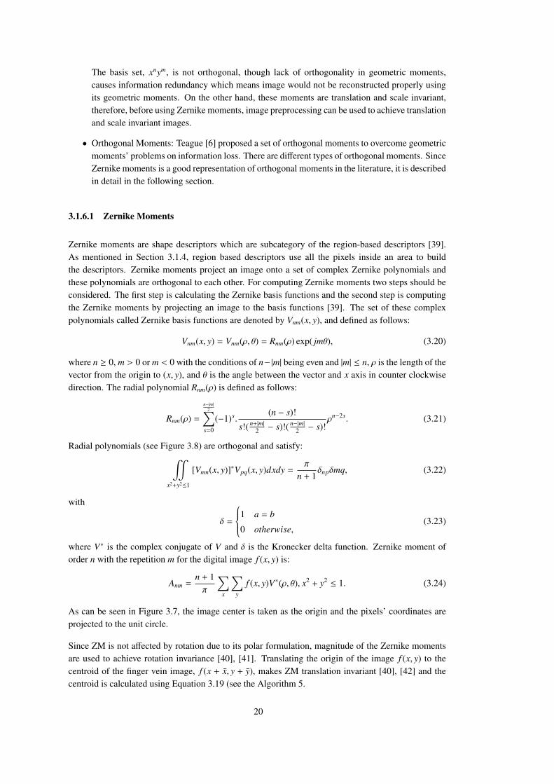
Since ZM is not affected by rotation due to its polar formulation, magnitude of the Zernike momentsare used to achieve rotation invariance [40], [41]. Translating the origin of the image f (x, y) to thecentroid of the finger vein image, f (x + x, y + y), makes ZM translation invariant [40], [42] and thecentroid is calculated using Equation 3.19 (see the Algorithm 5.

20

0 i N-1

j

N-1

1

-1

-1

1

Figure 3.7: Mapping transform (Source: [39]).

R00

R11

R51

R40

R31

R20

1

0.8

0.6

0.4

0.2

0

-0.2

-0.4

-0.6

-0.8

-10.1 0.2 0.3 0.4 0.5 0.6 0.7 0.8 0.9 1

Figure 3.8: Zernike radial polynomials of order 0-5 (Source: [39]).

21

Algorithm 5 Zernike Moments ComputationRequire: SZ: Size of the image, n: Order

Output: ZM: Zernike momentsradial← 0szh← S Z

2for x = 1 to S Z do

ρ←√

(szh − x)2 + (szh − y)2

θ ← tan−1( szh−yszh−x )

if ρ > szh thencontinue

end ifρ← ρ/szhfor s = 0 to n−size(m)

2 doradial← radial + (−1)s. (n−s)!

s!( n+size(m)2 −s)!( n−size(m)

2 −s)!ρn−2s

end for- Calculate Zernike Basis Function (ZBF):

ZBF ← radial × exp(n × θ × i j)end for

Calculate ZM using Equation 3.24

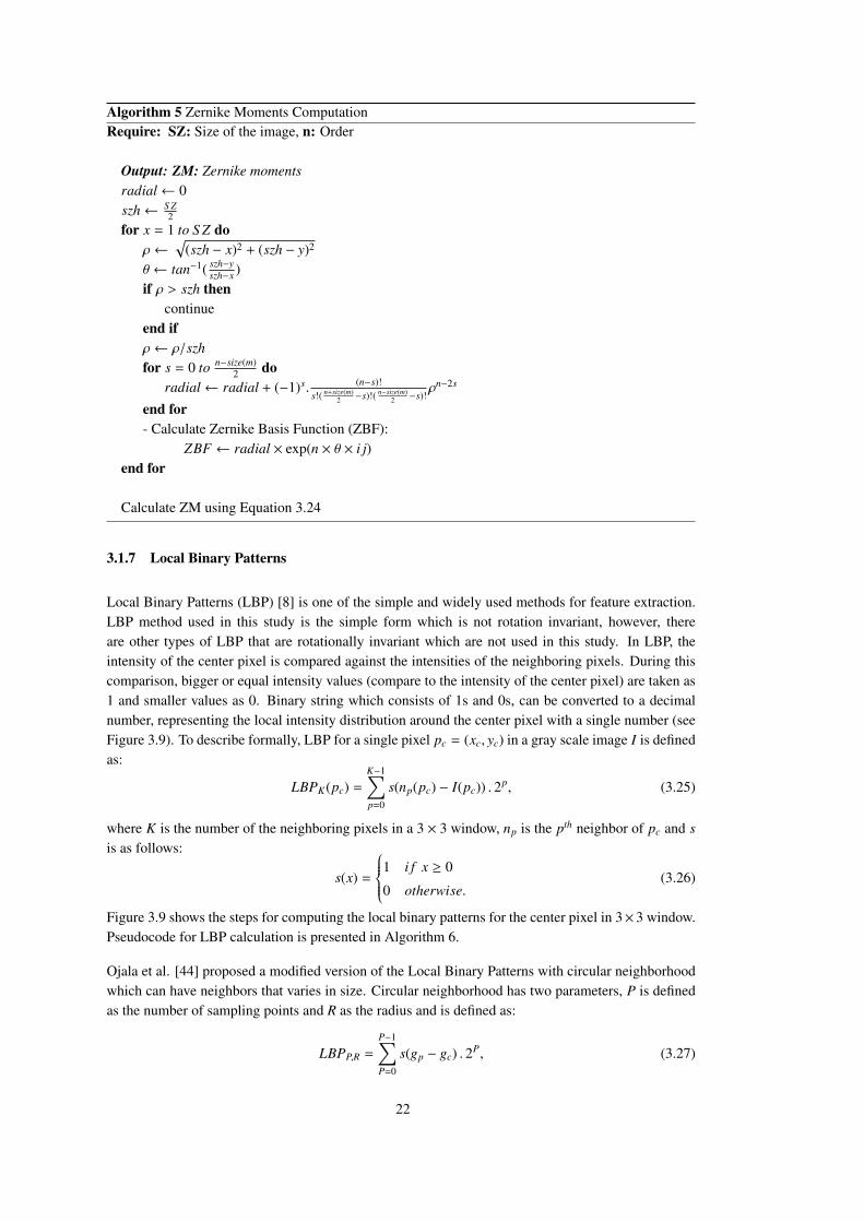
3.1.7 Local Binary Patterns

Local Binary Patterns (LBP) [8] is one of the simple and widely used methods for feature extraction.LBP method used in this study is the simple form which is not rotation invariant, however, thereare other types of LBP that are rotationally invariant which are not used in this study. In LBP, theintensity of the center pixel is compared against the intensities of the neighboring pixels. During thiscomparison, bigger or equal intensity values (compare to the intensity of the center pixel) are taken as1 and smaller values as 0. Binary string which consists of 1s and 0s, can be converted to a decimalnumber, representing the local intensity distribution around the center pixel with a single number (seeFigure 3.9). To describe formally, LBP for a single pixel pc = (xc, yc) in a gray scale image I is definedas:

LBPK(pc) =

K−1∑p=0

s(np(pc) − I(pc)) . 2p, (3.25)

where K is the number of the neighboring pixels in a 3 × 3 window, np is the pth neighbor of pc and sis as follows:

s(x) =

1 i f x ≥ 0

0 otherwise.(3.26)

Figure 3.9 shows the steps for computing the local binary patterns for the center pixel in 3×3 window.Pseudocode for LBP calculation is presented in Algorithm 6.

Ojala et al. [44] proposed a modified version of the Local Binary Patterns with circular neighborhoodwhich can have neighbors that varies in size. Circular neighborhood has two parameters, P is definedas the number of sampling points and R as the radius and is defined as:

LBPP,R =

P−1∑P=0

s(gp − gc) . 2P, (3.27)

22

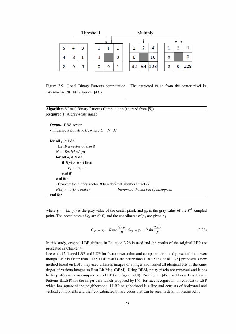
Figure 3.9: Local Binary Patterns computation. The extracted value from the center pixel is:

1+2+4+8+128=143 (Source: [43])

.

Algorithm 6 Local Binary Patterns Computation (adapted from [9])Require: I: A gray-scale image

Output: LBP vector- Initialize a L matrix H, where L = N · M

for all p ∈ I do- Let B a vector of size 8N ← 8neight(I, p)for all ni ∈ N do

if I(p) > I(ni) thenBi ← Bi + 1

end ifend for- Convert the binary vector B to a decimal number to get DH(k)← #{D ∈ bin(k)} - Increment the kth bin of histogram

end for

where gc = (xc, yc) is the gray value of the center pixel, and gp is the gray value of the Pth sampledpoint. The coordinates of gc are (0, 0) and the coordinates of gp are given by:

Cxp = xc + R cos2πp

P, Cyp = yc − R sin

2πpP. (3.28)

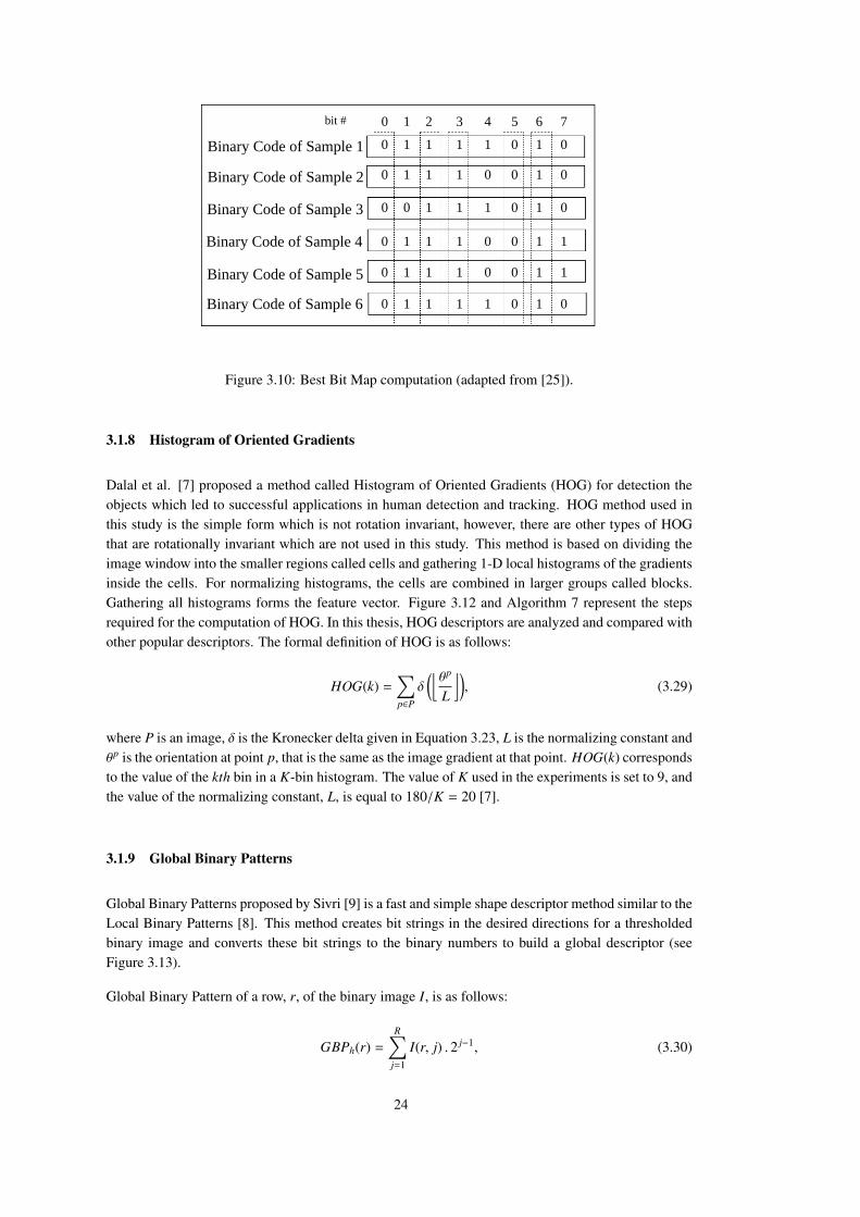
In this study, original LBP, defined in Equation 3.26 is used and the results of the original LBP arepresented in Chapter 4.Lee et al. [24] used LBP and LDP for feature extraction and compared them and presented that, eventhough LBP is faster than LDP, LDP results are better than LBP. Yang et al. [25] proposed a newmethod based on LBP; they used different images of a finger and named all identical bits of the samefinger of various images as Best Bit Map (BBM). Using BBM, noisy pixels are removed and it hasbetter performance in comparison to LBP (see Figure 3.10). Rosdi et al. [45] used Local Line BinaryPatterns (LLBP) for the finger vein which proposed by [46] for face recognition. In contrast to LBPwhich has square shape neighborhood, LLBP neighborhood is a line and consists of horizontal andvertical components and their concatenated binary codes that can be seen in detail in Figure 3.11.

23

Binary Code of Sample 1






bit # 0 1 2 3 4 5 6 7

0 1 1 1 1 0 1 0

0 1 1 1 0 0 1 0

0 0 1 1 1 0 1 0

0 1 1 1 0 0 1 1

0 1 1 1 0 0 1 1

0 1 1 1 1 0 1 0

Figure 3.10: Best Bit Map computation (adapted from [25]).

3.1.8 Histogram of Oriented Gradients

Dalal et al. [7] proposed a method called Histogram of Oriented Gradients (HOG) for detection theobjects which led to successful applications in human detection and tracking. HOG method used inthis study is the simple form which is not rotation invariant, however, there are other types of HOGthat are rotationally invariant which are not used in this study. This method is based on dividing theimage window into the smaller regions called cells and gathering 1-D local histograms of the gradientsinside the cells. For normalizing histograms, the cells are combined in larger groups called blocks.Gathering all histograms forms the feature vector. Figure 3.12 and Algorithm 7 represent the stepsrequired for the computation of HOG. In this thesis, HOG descriptors are analyzed and compared withother popular descriptors. The formal definition of HOG is as follows:

HOG(k) =∑p∈P

δ(⌊θp

L

⌋), (3.29)

where P is an image, δ is the Kronecker delta given in Equation 3.23, L is the normalizing constant andθp is the orientation at point p, that is the same as the image gradient at that point. HOG(k) correspondsto the value of the kth bin in a K-bin histogram. The value of K used in the experiments is set to 9, andthe value of the normalizing constant, L, is equal to 180/K = 20 [7].

3.1.9 Global Binary Patterns

Global Binary Patterns proposed by Sivri [9] is a fast and simple shape descriptor method similar to theLocal Binary Patterns [8]. This method creates bit strings in the desired directions for a thresholdedbinary image and converts these bit strings to the binary numbers to build a global descriptor (seeFigure 3.13).

Global Binary Pattern of a row, r, of the binary image I, is as follows:

GBPh(r) =

R∑j=1

I(r, j) . 2 j−1, (3.30)

24

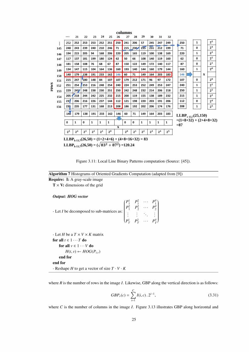
252 252 253 253 252 251 250 241 206 57 245 247 249

248 243 239 240 210 246 71 215 230 235 231 212 199

194 215 205 94 168 206 220 205 165 119 100 138 169

117 137 181 199 180 124 62 50 66 108 140 119 160

181 158 108 76 68 67 87 150 122 149 172 140 117

134 147 115 104 164 136 160 193 140 144 160 179 144

140 179 138 191 233 162 146 60 71 149 164 203 183

215 247 180 148 84 107 107 179 212 171 96 97 172

251 254 253 216 248 254 240 224 253 252 249 253 247

229 245 248 238 230 251 250 242 248 232 214 206 218

205 218 244 242 225 232 215 200 119 155 138 189 232

237 206 216 226 237 144 112 121 198 220 203 191 206

235 235 177 131 168 213 208 186 192 202 206 174 176

columns

row

s

… 21 22 23 24 25 26 27 28 29 30 31 32

…

153

146

147

148

149

150

151

152

145

154

155

156

250

71

220

62

87

160

146

107

240

250

215

112

208

1

0

1

0

0

1

0

1

1

1

0

1

𝟐𝟓

𝟐𝟒

𝟐𝟑

𝟐𝟐

𝟐𝟏

𝟐𝟎

𝟐𝟎

𝟐𝟏

𝟐𝟐

𝟐𝟑

𝟐𝟒

𝟐𝟓

140 179 138 191 233 162 146 60 71 149 164 203 183LLBPv 13,7(25,150)

=(1+8+32) + (2+4+8+32)

=870 1 0 1 1 1 0 0 1 1 1 1

𝟐𝟓 𝟐𝟒 𝟐𝟑 𝟐𝟐 𝟐𝟏 𝟐𝟎 𝟐𝟎 𝟐𝟏 𝟐𝟐 𝟐𝟑 𝟐𝟒 𝟐𝟓

LLBPh 13,7(26,50) = (1+2+4+6) + (4+8+16+32) = 83

LLBPh 13,7(26,50) = ( 𝟖𝟑𝟐 + 𝟖𝟕𝟐) =120.24

x

x

Figure 3.11: Local Line Binary Patterns computation (Source: [45]).

Algorithm 7 Histograms of Oriented Gradients Computation (adapted from [9])Require: I: A gray-scale image

T × V: dimensions of the grid

Output: HOG vector

- Let I be decomposed to sub-matrices as:

P1

1 P21 · · · PV

1P2

1 P22 · · · PV

2...

.... . .

...

P1T P2

T · · · PVT

- Let H be a T × V × K matrixfor all t ∈ 1 · · · T do

for all v ∈ 1 · · ·V doH(t, v)← HOG(Pt,v)

end forend for- Reshape H to get a vector of size T · V · K

where R is the number of rows in the image I. Likewise, GBP along the vertical direction is as follows:

GBPv(c) =

C∑i=1

I(i, c) . 2i−1, (3.31)

where C is the number of columns in the image I. Figure 3.13 illustrates GBP along horizontal and

25

Figure 3.12: Histogram of Oriented Gradients computation (Source: [47]).

vertical axis defined as GBPhv (see Algorithm 8). In order to calculate GBP along any direction withorientation θ (see Figure 3.14), the following equation can be used:

GBPθ(k) =∑p∈I

δ(L

xp −min(xpi j )max(xpi j ) −min(xpi j )

− k). I(P) . 2dp

, (3.32)

where δ is the Kronecker delta function, dp is the point-to-line distance between the line lp0θ and the

pixel p, projection of the pixel p onto the line lp0θ is xp and L is the length of the GBPθ descriptor. As

can be seen in Figure 3.14, lp0θ is the line with the orientation θ, which passes through p0. Horizontal

and vertical GBP are not invariant to rotation and translation.

Algorithm 8 Global Binary Patterns (GBPh) Computation (adapted from [9]).Require: I: R ×C thresholded image

Output: GBP vector- Let GBPh be a vector of size N

for all i ∈ 1 · · ·R dofor all j ∈ 1 · · ·C do

GBPh(i)← GBPh(i) + I(i, j) · 2 j−1

end forend for

3.2 Finger Vein Matching

Different matching methods have been used for matching the features extracted from each method. ForLT, MC and WL, the literature uses the so-called mismatch ratio in which a query map is comparedagainst a stored map pixel by pixel like (in template matching). For FD, ZM, HOG, LBP and GBP,many distance metrics are used in the literature, like Euclidean distance, χ2 distance and Earth Mover’sdistance. In this study, the mismatch ratio is used for LT, MC and WL, and Euclidean distance, χ2

distance and Earth Mover’s distance for FD, ZM, HOG, LBP and GBP.

26

0 0 1 1 1

0 1 0 1 0

1 1 0 1 0

0 1 0 0 0

0 0 1 1 0

0 0 22 23 24

0 21 0 0

20 0 0

0 0 0 0

0 0 0

23

23

2322

21

21

28

10

11

2

12

0 0 20 20 20

0 21 0 0

22 0 0

0 0 0 0

0 0 0

21

22

2424

22

23

4 14 17 23 1

4 14 17 23 128 10 11 2 12

Figure 3.13: GBP computation. (a) The binary image; (b) Rows are multiplied by powers of two;

(c) Each row is summed horizontally; (d) Columns are multiplied by powers of two; (e) Columns are

summed vertically; (f) Resulting GBP descriptor (Source: [9]).

Figure 3.14: Ilustration of GBP along an arbitrary direction with orientation θ (Source: [9]).

27

3.2.1 Template Matching

Template matching is one of the oldest and simplest methods in pattern recognition. In templatematching, the pattern to be identified is matched against the stored template [48]. Nm(s, t) which is thevalue of the mismatch is calculated as follows:

Nm(s, t) =

h−2ch−1∑y=0

w−2cw−1∑x=0

φ(I(s + x, t + y), R(cw + x, ch + y)

), (3.33)

where cw and ch are the distances for the variations in the horizontal and vertical directions, respectivelyand are used to adjust the displacement, w and h are the width and height of the images and φ(P1, P2)is defined as follows:

φ(P1, P2) =

1 i f |P1 − P2| = 255

0 otherwise.(3.34)

P1 is the pixel value of the image and P2 is the pixel value of the registered template.

Nm = min0≤s≤2cw,0≤t<2ch

(Nm(s, t)). (3.35)

The mismatch ratio, Rm, is calculated as follows:

Rm =Nm∑t0+h−2ch−1

j=t0

∑s0+w−2cw−1i=s0

φ(I(i, j), 0) +∑h−ch−1

j=ch

∑w−cw−1i=cw

φ(0,R(i, j)), (3.36)

where s0 and t0 are s and t that are minimized in Equation 3.35.

3.2.2 Euclidean Distance

The Euclidean distance between vectors X =

{xi

∣∣∣∣∣ i = 1, 2, ...,N}

and Y =

{yi

∣∣∣∣∣ i = 1, 2, ...,N}

are

defined as:

Euc(X,Y) =

√√ n∑i=1

(xi − yi)2. (3.37)

3.2.3 Chi-Square Distance (χ2)

X2 distance is a sub group of the Bin-By-Bin dissimilarity measures. The Bin-By-Bin dissimilaritymeasures pairs of the bins in two histograms that have the same index. This metric is used in wideareas such as shape classification and boundary detection [49].

χ2(X,Y) =12

∑i

(xi − yi)2

(xi + yi), (3.38)

where X =

{xi

∣∣∣∣∣ i = 1, 2, ...,N}

and Y =

{yi

∣∣∣∣∣ i = 1, 2, ...,N}

.

28

3.2.4 Earth Mover’s Distance (EMD)

Unlike the Bin-to-Bin dissimilarity in which corresponding histogram bins are compared, in Cross-Bindissimilarity, non-identical indexes of the bins are compared as well. Earth Mover’s Distance (EMD)is a solution to the transportation problem which defines the distance between two histograms and thegoal is to find the minimum cost when transforming one histogram to the other one [49]. The EMDbetween the two histograms, P = (pi, ui)m

i=1 and Q = (q j, v j)nj=1, where m and n are the size and the

flow between P and Q, which is shown with F = ( fi j), is calculated as follows:

EMD(P,Q) =

∑i, j fi j di j∑

i, j fi j, (3.39)

where di j is the ground distance matrix between pi and q j, ui and vi refer to the weights of the his-tograms and following constraints should be considered:

fi j ≥ 0,

where 1 ≤ i ≤ m, 1 ≤ j ≤ n,n∑

j=1

fi j ≤ ui,

where 1 ≤ i ≤ m,m∑

i=1

fi j ≤ v j,

where 1 ≤ j ≤ n, ∑i, j

fi j = min(∑

ui,∑

v j

).

29

30

CHAPTER 4

EXPERIMENTS

In the previous chapter the methods analyzed in the thesis were explained in detail and in this chapterthese methods are compared to each other and tested on their resilience against translation, rotationand noise. This is crucial since in finger vein image capturing systems, fingers tend to be not alignedthe same way each time they are scanned.In this chapter the database contents used in the experiments are explained and their performancesand running times are analyzed in depth. Used methods are Fourier descriptors (FD), Zernike mo-ments (ZM), Local Binary Patterns (LBP), Global Binary Patterns (GBP) and Histogram of OrientedGradients (HOG). Moreover, arbitrary N images are selected from the database which are translatedhorizontally for different shift amounts (0, 5, 10, 15 and 20 pixels) and rotated clockwise using nearestneighbor interpolation for different angles (0o, 5o, 10o, 15o and 20o) to analyze the methods againsttheir resistance to translation and rotation. Furthermore, Gaussian noise is added to the images. In thecase of Gaussian noise the variance has been investigated (0.0002, 0.0004, 0.0006, 0.0008 and 0.001)and the mean is kept zero (see Figure 4.1).The aim is to improve the running times and the resilience of LT, MC and WL using FD, ZM, HOG,LBP and GBP. It should be mentioned that these methods (FD, ZM, HOG, LBP and GBP) are appliedto the binarized locus table (from LT), the binarized Maximum Curvature map and the Wide LineDetector map.

4.1 The Database

The database in this study is carried out from SDUMLA-HMT finger-vein database that is publiclyavailable1. This database contains 3, 816 images from both hands and provided images are indexfinger, middle finger and ring finger and for each finger six different images are captured. Figure 4.2displays small sample of the database. The original images are of size 320×240, however, for the sakeof faster analysis, the size is reduced to 160 × 120 using nearest neighbor interpolation. The imagesare gray scale images in the intensity range of [0, 255].Using Prewitt edge detector, strong edges are extracted, the boundaries of the finger are found andthe mask image is produced (see Figure 4.3). Masking the image is a very important step since iteliminates the irrelevant areas.

1 http://mla.sdu.edu.cn/sdumla-hmt.html

31

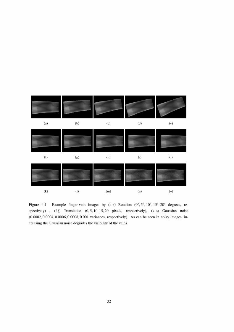
(a) (b) (c) (d) (e)

(f) (g) (h) (i) (j)

(k) (l) (m) (n) (o)

Figure 4.1: Example finger-vein images by (a-e) Rotation (0o, 5o, 10o, 15o, 20o degrees, re-

spectively) , (f-j) Translation (0, 5, 10, 15, 20 pixels, respectively), (k-o) Gaussian noise

(0.0002, 0.0004, 0.0006, 0.0008, 0.001 variances, respectively). As can be seen in noisy images, in-

creasing the Gaussian noise degrades the visibility of the veins.

32

Figure 4.2: Sample of Images from the SDUMLA-HMT Finger-vein Database

(a) (b) (c)

Figure 4.3: Finding the mask for the finger region in the image. (a) Original image, (b) Prewitt edge

detection, (c) Masked image.

4.2 Performance Measurement

Performances of algorithms are analyzed using Receiver Operating Characteristic (ROC) curve whichdepict the False Accepting Rates and the False Rejection Rates of an algorithm at the same time. Draw-ing a curve required calculating FAR and FRR for different threshold values (twenty threshold valuesare used in this study, different threshold values are calculated by dividing the subtract of maximumand minimum of the distances by twenty).

4.3 Results

The methods are compared based on the FAR and FRR, as widely used by the finger-vein recognitionliterature (e.g., Miura et al. [2]).

33

4.3.1 Line Tracking

Line Tracking method as outlined in Algorithm 1 has two main input parameters. The width of theprofiles are selected as w = 17 and the Radius as r = 1 based on the literature [2]. As can beseen in Figure 4.4, using the mask image locus table is produced and then by binarizing the locustable (using the median of the image as a threshold) finger veins are more emphasized. The LineTracking method is analyzed against rotation, translation and noise. For calculating the mismatchratio, displacement values are selected ch=50 and cw=30, which are the distances for the variations inthe vertical and horizontal directions, respectively and are used to adjust the displacement (see Section3.2.1). For this reason displacements are selected large enough therefore translation will not affect theLine Tracking method and as can be seen in Figure 4.5, Line Tracking method is translation invariantbut affected strongly by noise and rotation because of pixel by pixel comparison. The implementationof LT provided online at [50] is used in this thesis.

(a) (b) (c)

Figure 4.4: Example finger-vein extraction by the LT method. (a) Masked image, (b) Image extracted

from locus table, (c) Binarized version of (b) using median thresholding.

4.3.2 Maximum Curvature

The Maximum Curvature method as described in Algorithm 2 has just one parameter called S igma (σ)which is set σ = 3 based on the literature [3]. As can be seen in Figure 4.6, for extracting veins inthe Maximum Curvature method, the maximum curvature map is created and binarized (using themedian of the image as a threshold). The MC method analyzed against rotation, translation and noise.For calculating the mismatch ratio, displacement values are selected ch=50 and cw=30, which are thedistances for the variations in the vertical and horizontal directions, respectively and are used to adjustthe displacement (see Section 3.2.1). As can be seen in Figure 4.7, the Maximum Curvature method istranslation invariant because of selecting the displacement variables large enough (ch=50 and cw=30)and resistant to noise. However, this method is affected greatly by rotation because of changes in thegradient directions. The implementation of MC provided online at [50] is used in this thesis.

4.3.3 Wide Line Detector

Wide Line Detector method as explained in Algorithm 3 has three main parameters, two of whichare the threshold values (t=1, g=41) and the third one is Radius, which is set to r = 5 based on theliterature [4]. For extracting veins in the Wide Line Detector method, the WL map is created fromthe mask image (see Figure 4.8). For calculating the mismatch ratio, displacement values are selected

34

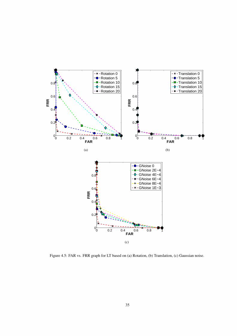
0 0.2 0.4 0.6 0.8 10

0.2

0.4

0.6

0.8

1

FAR

FR

R

Rotation 0Rotation 5Rotation 10Rotation 15Rotation 20

(a)

0 0.2 0.4 0.6 0.8 10

0.2

0.4

0.6

0.8

1

FAR

FR

R

Translation 0Translation 5Translation 10Translation 15Translation 20

(b)

0 0.2 0.4 0.6 0.8 10

0.2

0.4

0.6

0.8

1

FAR

FR

R

GNoise 0GNoise 2E−4GNoise 4E−4GNoise 6E−4GNoise 8E−4GNoise 1E−3

(c)

Figure 4.5: FAR vs. FRR graph for LT based on (a) Rotation, (b) Translation, (c) Gaussian noise.

35

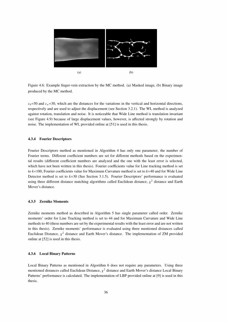
(a) (b)

Figure 4.6: Example finger-vein extraction by the MC method. (a) Masked image, (b) Binary image

produced by the MC method.

ch=50 and cw=30, which are the distances for the variations in the vertical and horizontal directions,respectively and are used to adjust the displacement (see Section 3.2.1). The WL method is analyzedagainst rotation, translation and noise. It is noticeable that Wide Line method is translation invariant(see Figure 4.9) because of large displacement values, however, is affected strongly by rotation andnoise. The implementation of WL provided online at [51] is used in this thesis.

4.3.4 Fourier Descriptors

Fourier Descriptors method as mentioned in Algorithm 4 has only one parameter; the number ofFourier terms. Different coefficient numbers are set for different methods based on the experimen-tal results (different coefficient numbers are analyzed and the one with the least error is selected,which have not been written in this thesis). Fourier coefficients value for Line tracking method is setto k=100, Fourier coefficients value for Maximum Curvature method is set to k=40 and for Wide LineDetector method is set to k=30 (See Section 3.1.5). Fourier Descriptors’ performance is evaluatedusing three different distance matching algorithms called Euclidean distance, χ2 distance and EarthMover’s distance.

4.3.5 Zernike Moments

Zernike moments method as described in Algorithm 5 has single parameter called order. Zernikemoments’ order for Line Tracking method is set to 44 and for Maximum Curvature and Wide Linemethods to 40 (these numbers are set by the experimental results with the least error and are not writtenin this thesis). Zernike moments’ performance is evaluated using three mentioned distances calledEuclidean Distance, χ2 distance and Earth Mover’s distance. The implementation of ZM providedonline at [52] is used in this thesis.

4.3.6 Local Binary Patterns

Local Binary Patterns as mentioned in Algorithm 6 does not require any parameters. Using threementioned distances called Euclidean Distance, χ2 distance and Earth Mover’s distance Local BinaryPatterns’ performance is calculated. The implementation of LBP provided online at [9] is used in thisthesis.

36

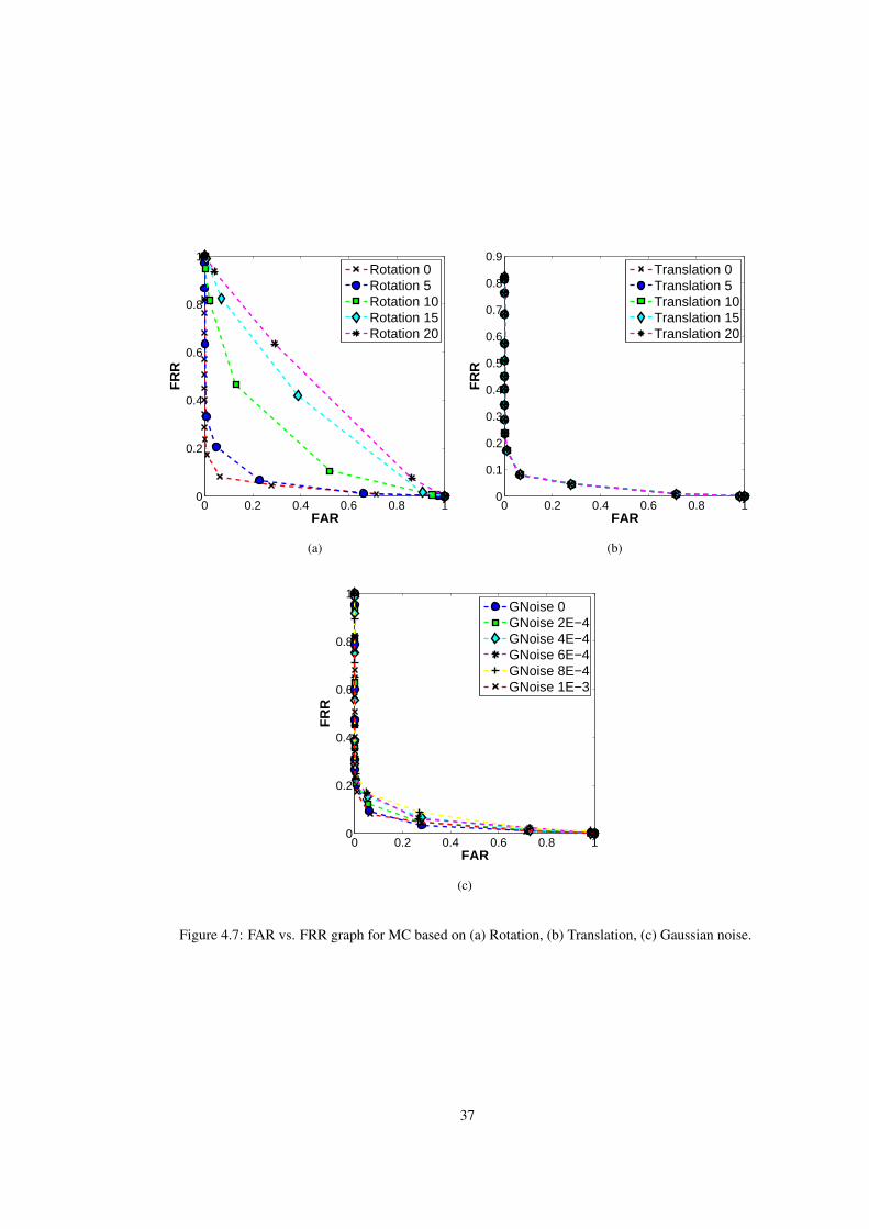
0 0.2 0.4 0.6 0.8 10

0.2

0.4

0.6

0.8

1

FAR

FR

R


(a)

0 0.2 0.4 0.6 0.8 10

0.1

0.2

0.3

0.4

0.5

0.6

0.7

0.8

0.9

FAR

FR

R


(b)

0 0.2 0.4 0.6 0.8 10

0.2

0.4

0.6

0.8

1

FAR

FR

R


(c)

Figure 4.7: FAR vs. FRR graph for MC based on (a) Rotation, (b) Translation, (c) Gaussian noise.

37

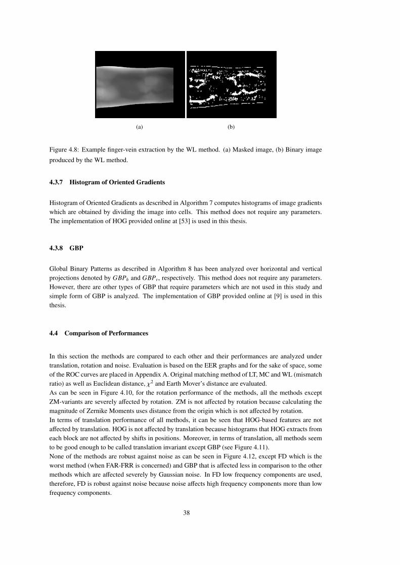
(a) (b)

Figure 4.8: Example finger-vein extraction by the WL method. (a) Masked image, (b) Binary image

produced by the WL method.

4.3.7 Histogram of Oriented Gradients

Histogram of Oriented Gradients as described in Algorithm 7 computes histograms of image gradientswhich are obtained by dividing the image into cells. This method does not require any parameters.The implementation of HOG provided online at [53] is used in this thesis.

4.3.8 GBP

Global Binary Patterns as described in Algorithm 8 has been analyzed over horizontal and verticalprojections denoted by GBPh and GBPv, respectively. This method does not require any parameters.However, there are other types of GBP that require parameters which are not used in this study andsimple form of GBP is analyzed. The implementation of GBP provided online at [9] is used in thisthesis.

4.4 Comparison of Performances

In this section the methods are compared to each other and their performances are analyzed undertranslation, rotation and noise. Evaluation is based on the EER graphs and for the sake of space, someof the ROC curves are placed in Appendix A. Original matching method of LT, MC and WL (mismatchratio) as well as Euclidean distance, χ2 and Earth Mover’s distance are evaluated.As can be seen in Figure 4.10, for the rotation performance of the methods, all the methods exceptZM-variants are severely affected by rotation. ZM is not affected by rotation because calculating themagnitude of Zernike Moments uses distance from the origin which is not affected by rotation.In terms of translation performance of all methods, it can be seen that HOG-based features are notaffected by translation. HOG is not affected by translation because histograms that HOG extracts fromeach block are not affected by shifts in positions. Moreover, in terms of translation, all methods seemto be good enough to be called translation invariant except GBP (see Figure 4.11).None of the methods are robust against noise as can be seen in Figure 4.12, except FD which is theworst method (when FAR-FRR is concerned) and GBP that is affected less in comparison to the othermethods which are affected severely by Gaussian noise. In FD low frequency components are used,therefore, FD is robust against noise because noise affects high frequency components more than lowfrequency components.

38

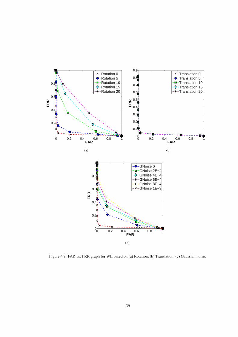
0 0.2 0.4 0.6 0.8 10

0.2

0.4

0.6

0.8

1

FAR

FR

R


(a)

0 0.2 0.4 0.6 0.8 10

0.1

0.2

0.3

0.4

0.5

0.6

0.7

0.8

0.9

FAR

FR

R


(b)

0 0.2 0.4 0.6 0.8 10

0.2

0.4

0.6

0.8

1

FAR

FR

R


(c)

Figure 4.9: FAR vs. FRR graph for WL based on (a) Rotation, (b) Translation, (c) Gaussian noise.

39

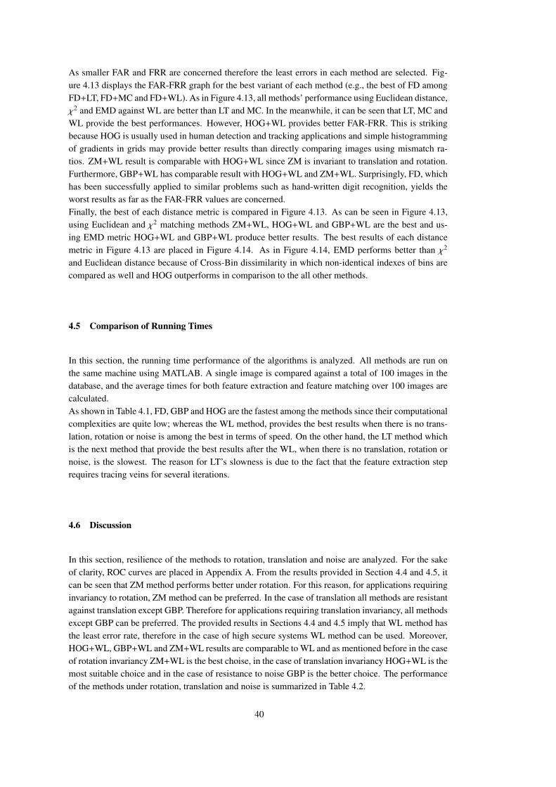
As smaller FAR and FRR are concerned therefore the least errors in each method are selected. Fig-ure 4.13 displays the FAR-FRR graph for the best variant of each method (e.g., the best of FD amongFD+LT, FD+MC and FD+WL). As in Figure 4.13, all methods’ performance using Euclidean distance,χ2 and EMD against WL are better than LT and MC. In the meanwhile, it can be seen that LT, MC andWL provide the best performances. However, HOG+WL provides better FAR-FRR. This is strikingbecause HOG is usually used in human detection and tracking applications and simple histogrammingof gradients in grids may provide better results than directly comparing images using mismatch ra-tios. ZM+WL result is comparable with HOG+WL since ZM is invariant to translation and rotation.Furthermore, GBP+WL has comparable result with HOG+WL and ZM+WL. Surprisingly, FD, whichhas been successfully applied to similar problems such as hand-written digit recognition, yields theworst results as far as the FAR-FRR values are concerned.Finally, the best of each distance metric is compared in Figure 4.13. As can be seen in Figure 4.13,using Euclidean and χ2 matching methods ZM+WL, HOG+WL and GBP+WL are the best and us-ing EMD metric HOG+WL and GBP+WL produce better results. The best results of each distancemetric in Figure 4.13 are placed in Figure 4.14. As in Figure 4.14, EMD performs better than χ2

and Euclidean distance because of Cross-Bin dissimilarity in which non-identical indexes of bins arecompared as well and HOG outperforms in comparison to the all other methods.

4.5 Comparison of Running Times

In this section, the running time performance of the algorithms is analyzed. All methods are run onthe same machine using MATLAB. A single image is compared against a total of 100 images in thedatabase, and the average times for both feature extraction and feature matching over 100 images arecalculated.As shown in Table 4.1, FD, GBP and HOG are the fastest among the methods since their computationalcomplexities are quite low; whereas the WL method, provides the best results when there is no trans-lation, rotation or noise is among the best in terms of speed. On the other hand, the LT method whichis the next method that provide the best results after the WL, when there is no translation, rotation ornoise, is the slowest. The reason for LT’s slowness is due to the fact that the feature extraction steprequires tracing veins for several iterations.

4.6 Discussion

In this section, resilience of the methods to rotation, translation and noise are analyzed. For the sakeof clarity, ROC curves are placed in Appendix A. From the results provided in Section 4.4 and 4.5, itcan be seen that ZM method performs better under rotation. For this reason, for applications requiringinvariancy to rotation, ZM method can be preferred. In the case of translation all methods are resistantagainst translation except GBP. Therefore for applications requiring translation invariancy, all methodsexcept GBP can be preferred. The provided results in Sections 4.4 and 4.5 imply that WL method hasthe least error rate, therefore in the case of high secure systems WL method can be used. Moreover,HOG+WL, GBP+WL and ZM+WL results are comparable to WL and as mentioned before in the caseof rotation invariancy ZM+WL is the best choise, in the case of translation invariancy HOG+WL is themost suitable choice and in the case of resistance to noise GBP is the better choice. The performanceof the methods under rotation, translation and noise is summarized in Table 4.2.

40

0 5 10 15 200

0.1

0.2

0.3

0.4

0.5

0.6

Rotation (degrees)

EE

R

LTMCWLFD+LTFD+MCFD+WLHOG+LTHOG+MCHOG+WLGBP+LTGBP+MCGBP+WLZM+LTZM+MCZM+WLLBP+LTLBP+MCLBP+WL

(a) Euclidean

0 5 10 15 200

0.1

0.2

0.3

0.4

0.5

0.6

Rotation (degrees)

EE

R


(b) χ2

0 5 10 15 200

0.1

0.2

0.3

0.4

0.5

0.6

Rotation (degrees)

EE

R


(c) EMD

Figure 4.10: Analysis of distance and rotation (a) Euclidean, (b) χ2, (c) EMD.

41

0 5 10 15 200

0.1

0.2

0.3

0.4

0.5

0.6

Translation (pixels)

EE

R


(a) Euclidean

0 5 10 15 200

0.1

0.2

0.3

0.4

0.5

0.6


EE

R


(b) χ2

0 5 10 15 200

0.1

0.2

0.3

0.4

0.5

0.6


EE

R


(c) EMD

Figure 4.11: Analysis of distance and translation (a) Euclidean, (b) χ2, (c) EMD.

42

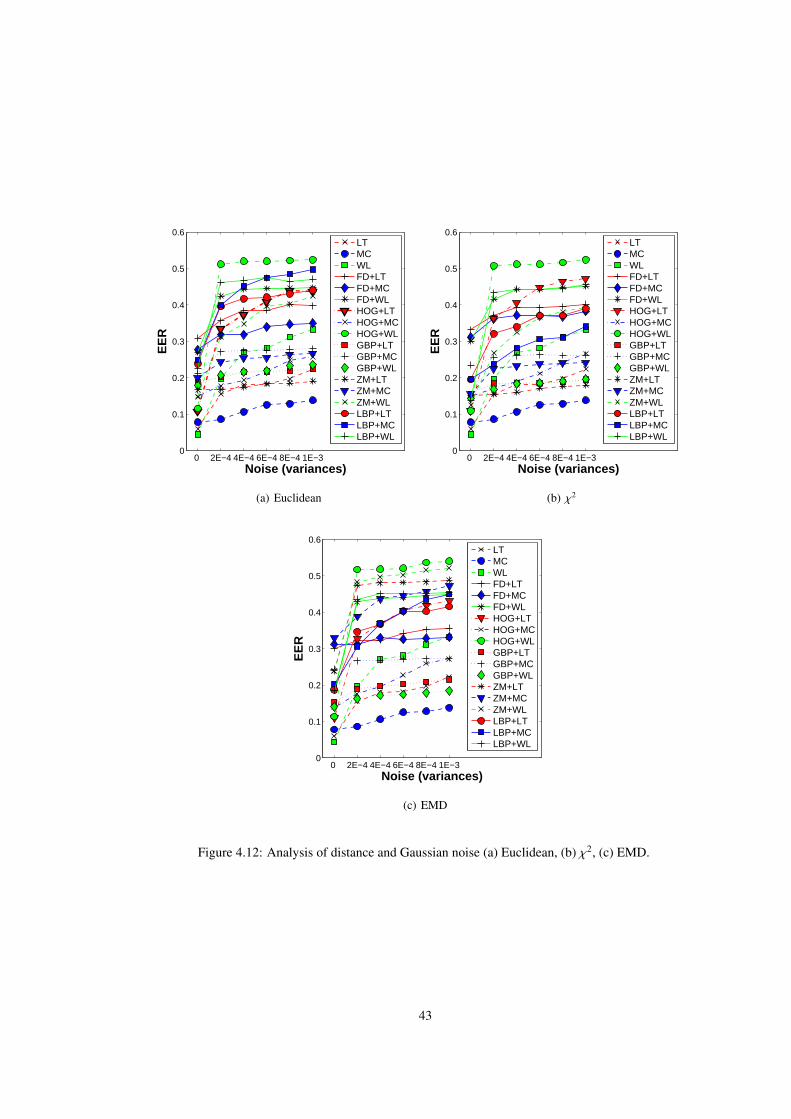
0 2E−4 4E−4 6E−4 8E−4 1E−30

0.1

0.2

0.3

0.4

0.5

0.6

Noise (variances)

EE

R


(a) Euclidean

0 2E−4 4E−4 6E−4 8E−4 1E−30

0.1

0.2

0.3

0.4

0.5

0.6

Noise (variances)

EE

R


(b) χ2

0 2E−4 4E−4 6E−4 8E−4 1E−30

0.1

0.2

0.3

0.4

0.5

0.6

Noise (variances)

EE

R


(c) EMD

Figure 4.12: Analysis of distance and Gaussian noise (a) Euclidean, (b) χ2, (c) EMD.

43

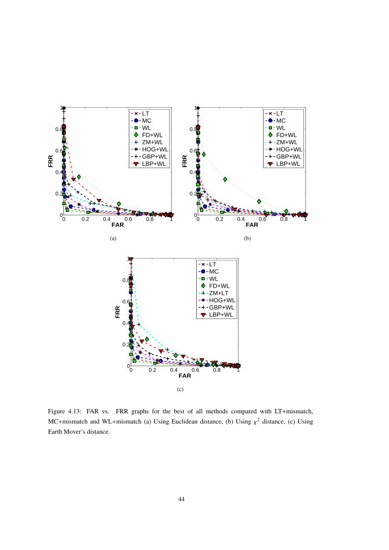
0 0.2 0.4 0.6 0.8 10

0.2

0.4

0.6

0.8

1

FAR

FR

R

LTMCWLFD+WLZM+WLHOG+WLGBP+WLLBP+WL

(a)

0 0.2 0.4 0.6 0.8 10

0.2

0.4

0.6

0.8

1

FAR

FR

R

LTMCWLFD+WLZM+WLHOG+WLGBP+WLLBP+WL

(b)

0 0.2 0.4 0.6 0.8 10

0.2

0.4

0.6

0.8

1

FAR

FR

R

LTMCWLFD+WLZM+LTHOG+WLGBP+WLLBP+WL

(c)

Figure 4.13: FAR vs. FRR graphs for the best of all methods compared with LT+mismatch,

MC+mismatch and WL+mismatch (a) Using Euclidean distance, (b) Using χ2 distance, (c) Using

Earth Mover’s distance.

44

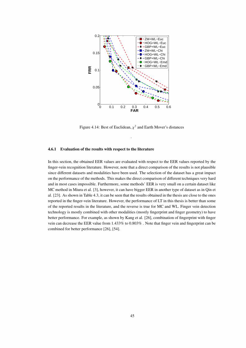
0 0.1 0.2 0.3 0.4 0.5 0.60

0.05

0.1

0.15

0.2

FAR

FR

R

ZM+WL−EucHOG+WL−EucGBP+WL−EucZM+WL−ChiHOG+WL−ChiGBP+WL−ChiHOG+WL−EmdGBP+WL−Emd

Figure 4.14: Best of Euclidean, χ2 and Earth Mover’s distances

.

4.6.1 Evaluation of the results with respect to the literature

In this section, the obtained EER values are evaluated with respect to the EER values reported by thefinger-vein recognition literature. However, note that a direct comparison of the results is not plausiblesince different datasets and modalities have been used. The selection of the dataset has a great impacton the performance of the methods. This makes the direct comparison of different techniques very hardand in most cases impossible. Furthermore, some methods’ EER is very small on a certain dataset likeMC method in Miura et al. [3], however, it can have bigger EER in another type of dataset as in Qin etal. [23]. As shown in Table 4.3, it can be seen that the results obtained in the thesis are close to the onesreported in the finger-vein literature. However, the performance of LT in this thesis is better than someof the reported results in the literature, and the reverse is true for MC and WL. Finger vein detectiontechnology is mostly combined with other modalities (mostly fingerprint and finger geometry) to havebetter performance. For example, as shown by Kang et al. [26], combination of fingerprint with fingervein can decrease the EER value from 1.433% to 0.803% . Note that finger vein and fingerprint can becombined for better performance [26], [54].

45

Table4.1: Running-time comparison of all methods.

Method Time (seconds) Speed Rank

LT (feat. extraction only) 9.2831 15

MC (feat. extraction only) 0.0585 1

WL (feat. extraction only) 0.1286 8

LT 9.4675 19

MC 0.0595 3

WL 0.1335 10

FD + LT + Euc 9.2837 16

FD + MC + Euc 0.0586 2

FD + WL + Euc 0.1289 9

ZM + LT + Euc 9.6507 21

ZM + MC + Euc 0.5183 7

ZM + WL + Euc 0.5920 14

GBP + LT + Euc 9.2850 17

GBP + MC + Euc 0.0601 4

GBP + WL + Euc 0.1454 12

HOG + LT + Euc 9.2925 18

HOG + MC + Euc 0.0664 5

HOG + WL + Euc 0.1368 11

LBP + LT + Euc 9.5831 20

LBP + MC + Euc 0.0890 6

LBP + WL + Euc 0.1686 13

Table4.2: Comparison of resilience to rotation, translation and noise

Methods Rotation Translation Noise

Fourier Descriptors Yes Yes Yes

Zernike Moments Yes Yes No

Local Binary Patterns No Yes No

Global Binary Patterns No No Yes

Histogram of Oriented Gradients No Yes No

46

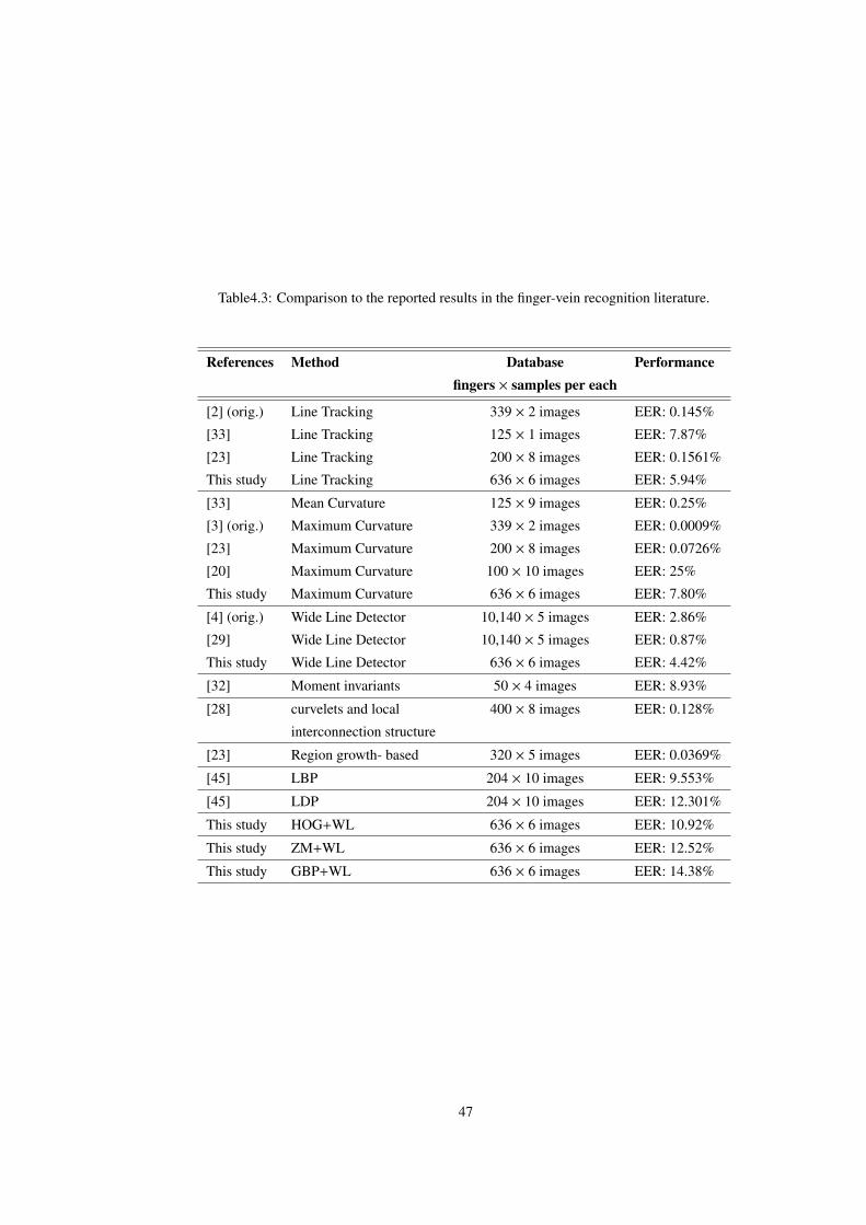
Table4.3: Comparison to the reported results in the finger-vein recognition literature.

References Method Database Performancefingers × samples per each

[2] (orig.) Line Tracking 339 × 2 images EER: 0.145%

[33] Line Tracking 125 × 1 images EER: 7.87%

[23] Line Tracking 200 × 8 images EER: 0.1561%

This study Line Tracking 636 × 6 images EER: 5.94%

[33] Mean Curvature 125 × 9 images EER: 0.25%

[3] (orig.) Maximum Curvature 339 × 2 images EER: 0.0009%

[23] Maximum Curvature 200 × 8 images EER: 0.0726%

[20] Maximum Curvature 100 × 10 images EER: 25%

This study Maximum Curvature 636 × 6 images EER: 7.80%

[4] (orig.) Wide Line Detector 10,140 × 5 images EER: 2.86%

[29] Wide Line Detector 10,140 × 5 images EER: 0.87%

This study Wide Line Detector 636 × 6 images EER: 4.42%

[32] Moment invariants 50 × 4 images EER: 8.93%

[28] curvelets and local 400 × 8 images EER: 0.128%

interconnection structure

[23] Region growth- based 320 × 5 images EER: 0.0369%

[45] LBP 204 × 10 images EER: 9.553%

[45] LDP 204 × 10 images EER: 12.301%

This study HOG+WL 636 × 6 images EER: 10.92%

This study ZM+WL 636 × 6 images EER: 12.52%

This study GBP+WL 636 × 6 images EER: 14.38%

47

48

CHAPTER 5

CONCLUSION

In this thesis, methods widely used for finger-vein recognition, namely, Line Tracking (LT), MaximumCurvature (MC) and Wide Line Detector (WL), are analyzed and extended for robustness againstrotation, translation and noise as well as faster running times. For this end, widely used ComputerVision and Pattern Recognition methods such as Fourier descriptors (FD), Zernike moments (ZM),Local Binary Patterns (LBP), Global Binary Patterns (GBP) and Histogram of Oriented Gradients(HOG) are used.It is observed that WL outperforms in terms of accuracy, however, it is affected by rotation and noise.Methods like ZM, HOG and GBP provide comparable performances and FD, HOG and GBP havebetter running times and ZM is invariant to rotation and translation, however, its running time is slowerthan HOG and GBP. Fourier descriptors are robust against noise, however, the error rate is very high.On the other hand, all other methods are affected strongly by noise except GBP.The results indicate that in the case of no noise, no rotation and no translation, WL is the best method.In a scenario involving rotation, ZM+WL, and in a scenario involving noise GBP+WL can be used. Iftime is a critical issue, then MC can be chosen since it is the next best method in terms of EER valuesand the fastest among all methods.

5.1 Future Work

There are different feature description methods in the literature that can be analyzed. For example,there are extensions of LBP, HOG and GBP that provide several invariances, such as rotation invari-ance, scale invariance. These extensions are worth analyzing as future work. For analyzing resilienceto rotation and translation, rotating the finger in different directions and axes will be much realistic,moreover, changing the distance between the finger and camera can be tested instead of artificiallyrotating, translating and adding noise to the images.In the thesis, only one database is used for analyzing the performance of the methods. However, forbetter evaluation and analysis, other databases, especially those with more images and more distortionsshould be used.For better analysis of the parameters and the performances of the methods Statistical Package for theSocial Sciences (SPSS) software can be used as a future work.

49

50

REFERENCES

[1] Hemant Vallabh. Authentication using finger-vein recognition. PhD thesis, University of Johan-

nesburg, 2013.

[2] Naoto Miura, Akio Nagasaka, and Takafumi Miyatake. Feature extraction of finger-vein patterns

based on repeated line tracking and its application to personal identification. Machine Vision and

Applications, 15(4):194–203, 2004.

[3] Naoto Miura, Akio Nagasaka, and Takafumi Miyatake. Extraction of finger-vein patterns using

maximum curvature points in image profiles. IEICE Transactions on Information and Systems,

90(8):1185–1194, 2007.

[4] Beining Huang, Yanggang Dai, Rongfeng Li, Darun Tang, and Wenxin Li. Finger-vein authen-

tication based on wide line detector and pattern normalization. In 20th International Conference

on Pattern Recognition (ICPR), pages 1269–1272. IEEE, 2010.

[5] Rafael C Gonzalez, Richard E Woods, and Steven L Eddins. Digital image processing using

MATLAB, volume 2. Gatesmark Publishing Knoxville, 2009.

[6] Michael R Teague. Image analysis via the general theory of moments. Journal of Optical Society

of America (JOSA), 70(8):920–930, 1980.

[7] Navneet Dalal and Bill Triggs. Histograms of oriented gradients for human detection. In IEEE

Computer Society Conference on Computer Vision and Pattern Recognition (CVPR), volume 1,

pages 886–893. IEEE, 2005.

[8] Timo Ojala, Matti Pietikäinen, and David Harwood. A comparative study of texture measures

with classification based on featured distributions. Pattern recognition, 29(1):51–59, 1996.

[9] Erdal Sivri. Shape descriptors based on intersection consistency and global binary patterns.

Master’s thesis, Middle East Technical University, Ankara, Turkey, 2012.

[10] David C Hitchcock. Evaluation and combination of biometric authentication systems. PhD

thesis, University of Florida, 2003.

[11] John D Woodward, Nicholas M Orlans, and Peter T Higgins. Biometrics:[identity assurance in

the information age]. McGraw-Hill/Osborne Berkeley, California, USA, 2003.

[12] Anil K Jain, Ruud M Bolle, and Sharath Pankanti. Biometrics: personal identification in net-

worked society. Springer, 1999.

[13] Thiems Nanavati. Biometrics. John Wiley & Sons, 2002.

51

[14] Sargur N Srihari, Harish Srinivasan, and Gang Fang. Discriminability of fingerprints of twins.

Journal of Forensic Identification, 58(1):109, 2008.

[15] Takashi Yanagawa, Satoshi Aoki, and Tetsuji Ohyama. Human finger vein images are diverse

and its patterns are useful for personal identification. 2007-12, 2007.

[16] Jinfeng Yang, Yihua Shi, Jinli Yang, and Lihui Jiang. A novel finger-vein recognition method

with feature combination. In 16th IEEE International Conference on Image Processing (ICIP),

pages 2709–2712. IEEE, 2009.

[17] Jinfeng Yang, Yihua Shi, and Jinli Yang. Personal identification based on finger-vein features.

Computers in Human Behavior, 27(5):1565–1570, 2011.

[18] Jinfeng Yang and Yihua Shi. Finger–vein roi localization and vein ridge enhancement. Pattern

Recognition Letters, 33(12):1569–1579, 2012.

[19] Wang Kejun, Liu Jingyu, Popoola P Oluwatoyin, and Feng Weixing. Finger vein identifica-

tion based on 2-d gabor filter. In 2nd International Conference on Industrial Mechatronics and

Automation (ICIMA), volume 2, pages 10–13. IEEE, 2010.

[20] Jinfeng Yang and Xu Li. Efficient finger vein localization and recognition. In 20th International

Conference on Pattern Recognition (ICPR), pages 1148–1151. IEEE, 2010.

[21] Li Xueyan, Guo Shuxu, Gao Fengli, and Li Ye. Vein pattern recognitions by moment invariants.

In The 1st International Conference on Bioinformatics and Biomedical Engineering (ICBBE),

pages 612–615. IEEE, 2007.

[22] Nurhafizah Mahri, Sas Suandi, and Bakhtiar A Rosdi. Finger vein recognition algorithm using

phase only correlation. In 2010 International Workshop on Emerging Techniques and Challenges

for Hand-Based Biometrics (ETCHB), pages 1–6. IEEE, 2010.

[23] Huafeng Qin, Lan Qin, and Chengbo Yu. Region growth–based feature extraction method for

finger-vein recognition. Optical Engineering, 50(5):057208–057208, 2011.

[24] Eui C Lee, Hyunwoo Jung, and Daeyeoul Kim. New finger biometric method using near infrared

imaging. Sensors, 11(3):2319–2333, 2011.

[25] Gongping Yang, Xiaoming Xi, and Yilong Yin. Finger vein recognition based on a personalized

best bit map. Sensors, 12(2):1738–1757, 2012.

[26] Byung J Kang, Kang R Park, Jang H Yoo, and Jeong N Kim. Multimodal biometric method that

combines veins, prints, and shape of a finger. Optical Engineering, 50(1):017201–017201, 2011.

[27] Leila Mirmohamadsadeghi and Andrzej Drygajlo. Palm vein recognition with local binary pat-

terns and local derivative patterns. In International Joint Conference on Biometrics (IJCB), pages

1–6. IEEE, 2011.

[28] Zhongbo Zhang, Siliang Ma, and Xiao Han. Multiscale feature extraction of finger-vein patterns

based on curvelets and local interconnection structure neural network. In 18th International

Conference on Pattern Recognition (ICPR), volume 4, pages 145–148. IEEE, 2006.

52

[29] Gongping Yang, Xiaoming Xi, and Yilong Yin. Finger vein recognition based on (2d)2 pca and

metric learning. Journal of Biomedicine and Biotechnology, 2012:9, 2012.

[30] Naoto Miura, Akio Nagasaka, and Takafumi Miyatake. Automatic feature extraction from non-

uniform finger vein image and its application to personal identification. In Machine Vision Ap-

plications (MVA), pages 253–256, 2002.

[31] Wenming Yang, Xiang Yu, and Qingmin Liao. Personal authentication using finger vein pattern

and finger-dorsa texture fusion. In Proceedings of the 17th ACM international conference on

Multimedia, pages 905–908. ACM, 2009.

[32] Xiaohua Qian, Shuxu Guo, Xueyan Li, Fei Zhong, and Xiangxin Shao. Finger-vein recognition

based on the score level moment invariants fusion. In International Conference on Computa-

tional Intelligence and Software Engineering (CiSE), pages 1–4. IEEE, 2009.

[33] Wonseok Song, Taejeong Kim, Hee C Kim, Joon H Choi, Hyoun J Kong, and Seung R Lee. A

finger-vein verification system using mean curvature. Pattern Recognition Letters, 32(11):1541–

1547, 2011.

[34] Jiang Hong, Guo Shuxu, Li Xueyan, and Qian Xiaohua. Vein pattern extraction based on the

position-gray-profile curve. In 2nd International Congress on Image and Signal Processing

(CISP), pages 1–4. IEEE, 2009.

[35] Laura Liu, David Zhang, and Jane You. Detecting wide lines using isotropic nonlinear filtering.

IEEE Transactions on Image Processing, 16(6):1584–1595, 2007.

[36] Lionel Evina Ekombo, Noureddine Ennahnahi, Mohammed Oumsis, and Mohammed Meknassi.

Application of affine invariant fourier descriptor to shape based image retrieval. International

Journal of Computer Science and Network Security, 9(7):240–247, 2009.

[37] Berrin Yanikoglu and Alisher Kholmatov. Online signature verification using fourier descriptors.

Journal on Advances in Signal Processing (EURASIP), 2009:12, 2009.

[38] Ming K Hu. Visual pattern recognition by moment invariants. IRE Transactions on Information

Theory, 8(2):179–187, 1962.

[39] Sun K Hwang and Whoi Y Kim. A novel approach to the fast computation of zernike moments.

Pattern Recognition, 39(11):2065–2076, 2006.

[40] Alireza Khotanzad and Yaw H Hong. Invariant image recognition by zernike moments. IEEE

Transactions on Pattern Analysis and Machine Intelligence, 12(5):489–497, 1990.

[41] Amir Tahmasbi, Fatemeh Saki, and Shahriar B Shokouhi. Classification of benign and malignant

masses based on zernike moments. Computers in Biology and Medicine, 41(8):726–735, 2011.

[42] Chee W Chong, Paramesran Raveendran, and Ramakrishnan Mukundan. Translation invariants

of zernike moments. Pattern Recognition, 36(8):1765–1773, 2003.

53

[43] Topi Mäenpää and Matti Pietikäinen. Texture analysis with local binary patterns. Handbook of

Pattern Recognition and Computer Vision, 3:197–216, 2005.

[44] Timo Ojala, Matti Pietikainen, and Topi Maenpaa. Multiresolution gray-scale and rotation in-

variant texture classification with local binary patterns. IEEE Transactions on Pattern Analysis

and Machine Intelligence, 24(7):971–987, 2002.

[45] Bakhtiar A Rosdi, Chai W Shing, and Shahrel A Suandi. Finger vein recognition using local line

binary pattern. Sensors, 11(12):11357–11371, 2011.

[46] Amnart Petpon and Sanun Srisuk. Face recognition with local line binary pattern. In Fifth

International Conference on Image and Graphics (ICIG), pages 533–539. IEEE, 2009.

[47] Tatsuo Kozakaya, Tomoyuki Shibata, Mayumi Yuasa, and Osamu Yamaguchi. Facial fea-

ture localization using weighted vector concentration approach. Image and Vision Computing,

28(5):772–780, 2010.

[48] Anil K Jain, Robert P Duin, and Jianchang Mao. Statistical pattern recognition: A review. IEEE

Transactions on Pattern Analysis and Machine Intelligence, 22(1):4–37, 2000.

[49] Yossi Rubner, Carlo Tomasi, and Leonidas J Guibas. The earth mover’s distance as a metric for

image retrieval. International Journal of Computer Vision, 40(2):99–121, 2000.

[50] Line Tracking and Maximum Curvature methods matlab code. http://www.mathworks.com/

matlabcentral/fileexchange/35716-miura-et-al-vein-extraction-methods. Ac-

cessed: 2012-12-10.

[51] Wide Line method matlab code. http://www.mathworks.com/matlabcentral/

fileexchange/35754-wide-line-detector. Accessed: 2012-12-20.

[52] Zernike moment method matlab code. http://liris.cnrs.fr/christian.wolf/

software/zernike/index.html. Accessed: 2013-01-15.

[53] Histogram of Oriented Gradient method matlab code. http://www.mathworks.com/

matlabcentral/fileexchange/33863-histograms-of-oriented-gradients. Ac-

cessed: 2013-07-10.

[54] Beyun J Kang and Kang R Park. Multimodal biometric method based on vein and geometry of a

single finger. IET Computer Vision, 4(3):209–217, 2010.

54

http://www.mathworks.com/matlabcentral/fileexchange/35716-miura-et-al-vein-extraction-methods

http://www.mathworks.com/matlabcentral/fileexchange/35716-miura-et-al-vein-extraction-methods

http://www.mathworks.com/matlabcentral/fileexchange/35754-wide-line-detector

http://www.mathworks.com/matlabcentral/fileexchange/35754-wide-line-detector

http://liris.cnrs.fr/christian.wolf/software/zernike/index.html

http://liris.cnrs.fr/christian.wolf/software/zernike/index.html

http://www.mathworks.com/matlabcentral/fileexchange/33863-histograms-of-oriented-gradients

http://www.mathworks.com/matlabcentral/fileexchange/33863-histograms-of-oriented-gradients

APPENDIX A

DETAILED RESULTS ON THE PERFORMANCE OF THEMETHODS

In this section performance of the methods are analyzed in detail and the results are based on the ROCcurves. Figures illustrate the affect of rotation, translation and noise on the methods including FD,ZM, HOG, LBP and GBP. As mentioned before in Section 4, arbitrary N images are selected from thedatabase which are translated horizontally for different shift amounts (0, 5, 10, 15 and 20 pixels) androtated clockwise for different angles (0o, 5o, 10o, 15o and 20o) to analyze the methods against theirresistance to translation and rotation. Furthermore, Gaussian noise is added to the images, where thevariance of the Gaussian was in the set (0.0002, 0.0004, 0.0006, 0.0008 and 0.001) and the mean waskept zero.As can be seen in Figures A.46, A.47 and A.48, FD, ZM, HOG, LBP and GBP are applied to LT, MCand WL and it is noticeable that WL outperforms all other methods.ZM method performs better under rotation as discussed in Section 4.6 , therefore can be used in theapplications requiring invariancy to rotation. In the case of translation all methods are resistant againsttranslation except GBP. However, GBP is resistant against noise and all other methods are affectedgreatly under noise (figure numbers are not provided here since there are many figures).

55

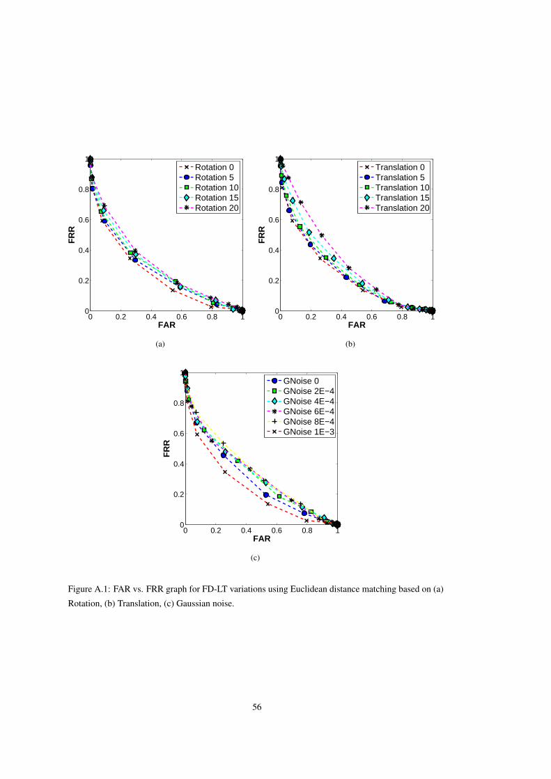
0 0.2 0.4 0.6 0.8 10

0.2

0.4

0.6

0.8

1

FAR

FR

R


(a)

0 0.2 0.4 0.6 0.8 10

0.2

0.4

0.6

0.8

1

FAR

FR

R


(b)

0 0.2 0.4 0.6 0.8 10

0.2

0.4

0.6

0.8

1

FAR

FR

R


(c)

Figure A.1: FAR vs. FRR graph for FD-LT variations using Euclidean distance matching based on (a)

Rotation, (b) Translation, (c) Gaussian noise.

56

0 0.2 0.4 0.6 0.8 10

0.2

0.4

0.6

0.8

1

FAR

FR

R


(a)

0 0.2 0.4 0.6 0.8 10

0.2

0.4

0.6

0.8

1

FAR

FR

R


(b)

0 0.2 0.4 0.6 0.8 10

0.2

0.4

0.6

0.8

1

FAR

FR

R


(c)

Figure A.2: FAR vs. FRR graph for FD-LT variations using χ2 distance matching based on (a) Rota-

tion, (b) Translation, (c) Gaussian noise.

57

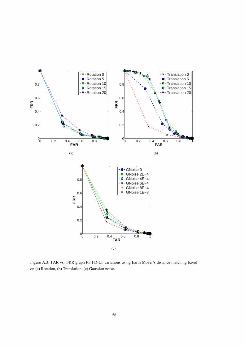
0 0.2 0.4 0.6 0.8 10

0.2

0.4

0.6

0.8

1

FAR

FR

R


(a)

0 0.2 0.4 0.6 0.8 10

0.2

0.4

0.6

0.8

1

FAR

FR

R


(b)

0 0.2 0.4 0.6 0.8 10

0.2

0.4

0.6

0.8

1

FAR

FR

R


(c)

Figure A.3: FAR vs. FRR graph for FD-LT variations using Earth Mover’s distance matching based

on (a) Rotation, (b) Translation, (c) Gaussian noise.

58

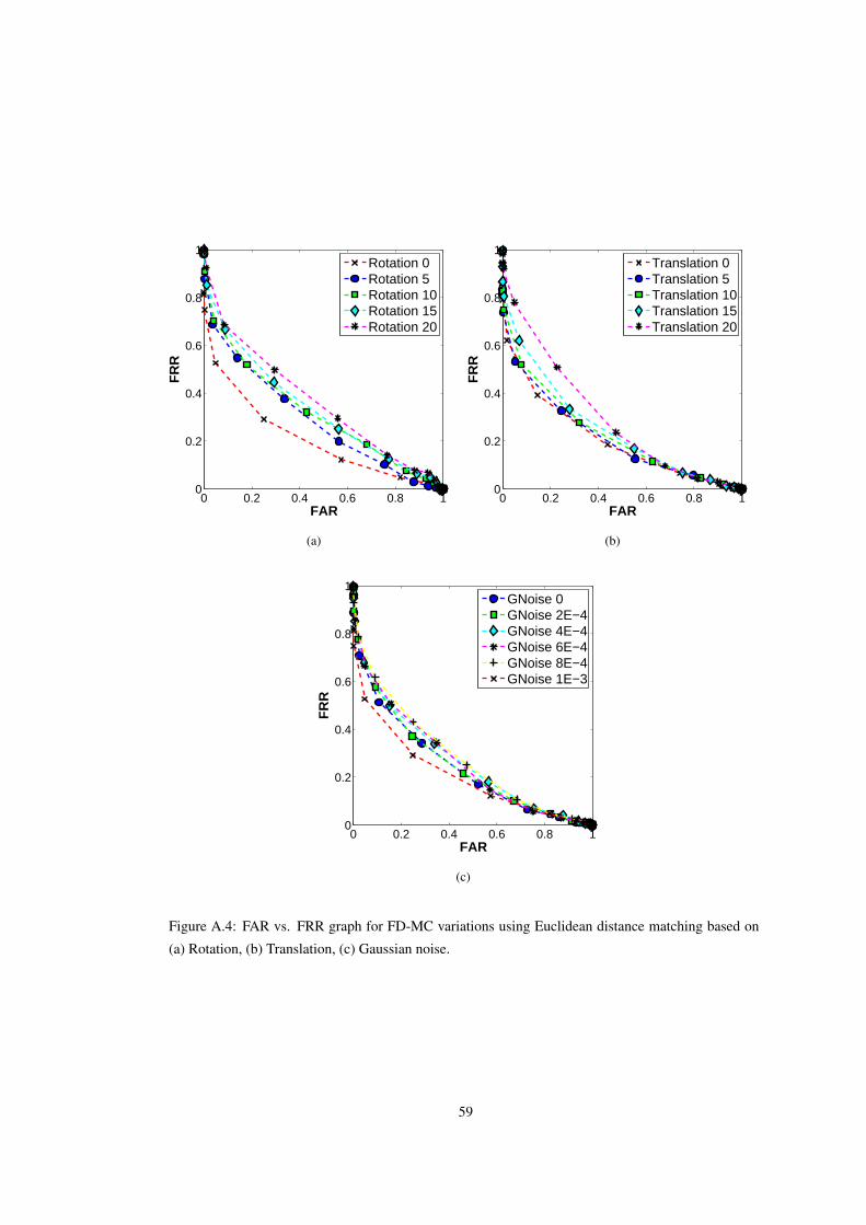
0 0.2 0.4 0.6 0.8 10

0.2

0.4

0.6

0.8

1

FAR

FR

R


(a)

0 0.2 0.4 0.6 0.8 10

0.2

0.4

0.6

0.8

1

FAR

FR

R


(b)

0 0.2 0.4 0.6 0.8 10

0.2

0.4

0.6

0.8

1

FAR

FR

R


(c)

Figure A.4: FAR vs. FRR graph for FD-MC variations using Euclidean distance matching based on

(a) Rotation, (b) Translation, (c) Gaussian noise.

59

0 0.2 0.4 0.6 0.8 10

0.2

0.4

0.6

0.8

1

FAR

FR

R


(a)

0 0.2 0.4 0.6 0.8 10

0.2

0.4

0.6

0.8

1

FAR

FR

R


(b)

0 0.2 0.4 0.6 0.8 10

0.2

0.4

0.6

0.8

1

FAR

FR

R


(c)

Figure A.5: FAR vs. FRR graph for FD-MC variations using χ2 distance matching based on (a)


60

0 0.2 0.4 0.6 0.8 10

0.2

0.4

0.6

0.8

1

FAR

FR

R


(a)

0 0.2 0.4 0.6 0.8 10

0.2

0.4

0.6

0.8

1

FAR

FR

R


(b)

0 0.2 0.4 0.6 0.8 10

0.2

0.4

0.6

0.8

1

FAR

FR

R


(c)

Figure A.6: FAR vs. FRR graph for FD-MC variations using Earth Mover’s distance matching based


61

0 0.2 0.4 0.6 0.8 10

0.2

0.4

0.6

0.8

1

FAR

FR

R


(a)

0 0.2 0.4 0.6 0.8 10

0.2

0.4

0.6

0.8

1

FAR

FR

R


(b)

0 0.2 0.4 0.6 0.8 10

0.2

0.4

0.6

0.8

1

FAR

FR

R


(c)

Figure A.7: FAR vs. FRR graph for FD-WL variations using Euclidean distance matching based on


62

0 0.2 0.4 0.6 0.8 10

0.2

0.4

0.6

0.8

1

FAR

FR

R


(a)

0 0.2 0.4 0.6 0.8 10

0.2

0.4

0.6

0.8

1

FAR

FR

R


(b)

0 0.2 0.4 0.6 0.8 10

0.2

0.4

0.6

0.8

1

FAR

FR

R


(c)

Figure A.8: FAR vs. FRR graph for FD-WL variations using χ2 distance matching based on (a)


63

0 0.2 0.4 0.6 0.8 10

0.2

0.4

0.6

0.8

1

FAR

FR

R


(a)

0 0.2 0.4 0.6 0.8 10

0.2

0.4

0.6

0.8

1

FAR

FR

R


(b)

0 0.2 0.4 0.6 0.8 10

0.2

0.4

0.6

0.8

1

FAR

FR

R


(c)

Figure A.9: FAR vs. FRR graph for FD-WL variations using Earth Mover’s distance matching based


64

0 0.2 0.4 0.6 0.8 10

0.2

0.4

0.6

0.8

1

FAR

FR

R


(a)

0 0.2 0.4 0.6 0.8 10

0.2

0.4

0.6

0.8

1

FAR

FR

R


(b)

0 0.2 0.4 0.6 0.8 10

0.2

0.4

0.6

0.8

1

FAR

FR

R


(c)

Figure A.10: FAR vs. FRR graph for ZM-LT variations using Euclidean distance matching based on


65

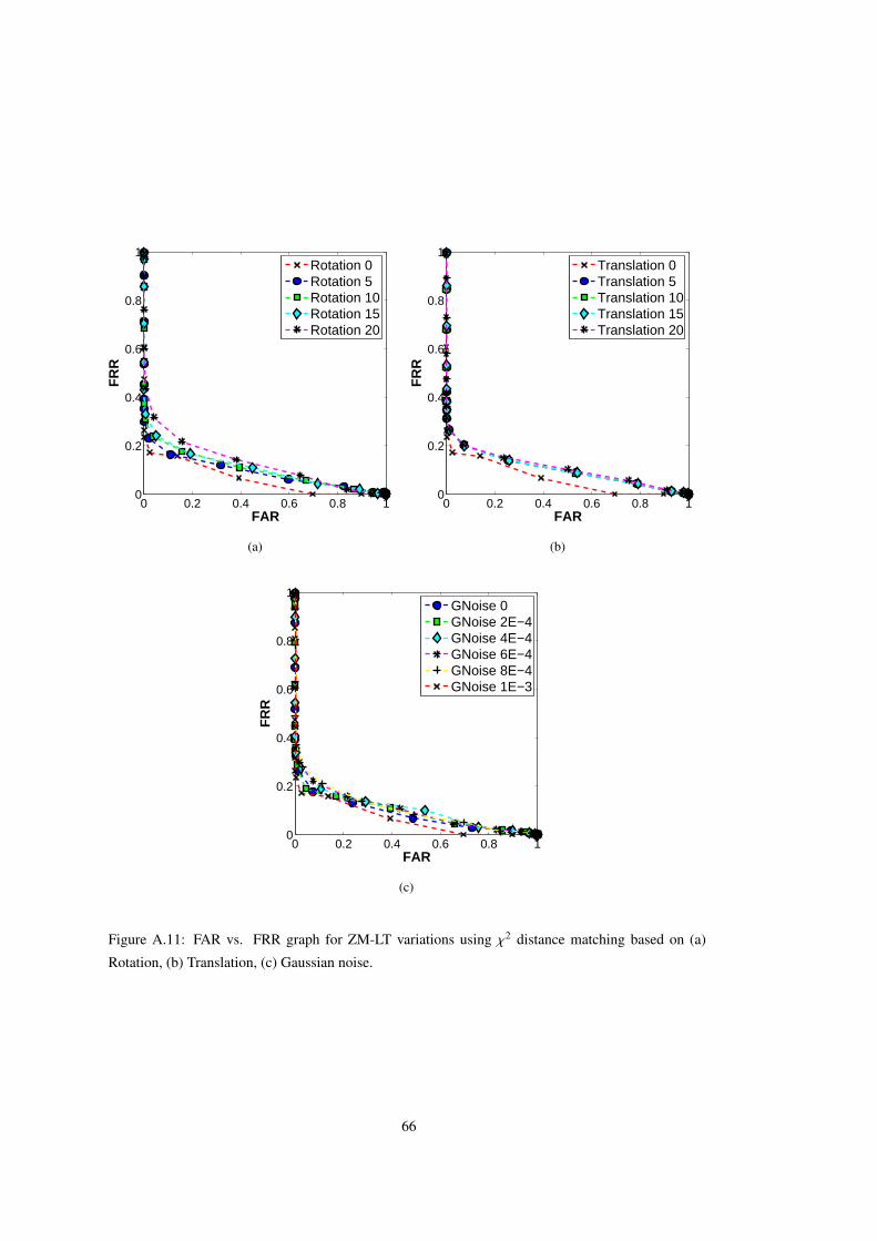
0 0.2 0.4 0.6 0.8 10

0.2

0.4

0.6

0.8

1

FAR

FR

R


(a)

0 0.2 0.4 0.6 0.8 10

0.2

0.4

0.6

0.8

1

FAR

FR

R


(b)

0 0.2 0.4 0.6 0.8 10

0.2

0.4

0.6

0.8

1

FAR

FR

R


(c)

Figure A.11: FAR vs. FRR graph for ZM-LT variations using χ2 distance matching based on (a)


66

0 0.2 0.4 0.6 0.8 10

0.2

0.4

0.6

0.8

1

FAR

FR

R


(a)

0 0.2 0.4 0.6 0.8 10

0.2

0.4

0.6

0.8

1

FAR

FR

R


(b)

0 0.2 0.4 0.6 0.8 10

0.2

0.4

0.6

0.8

1

FAR

FR

R


(c)

Figure A.12: FAR vs. FRR graph for ZM-LT variations using Earth Mover’s distance matching based


67

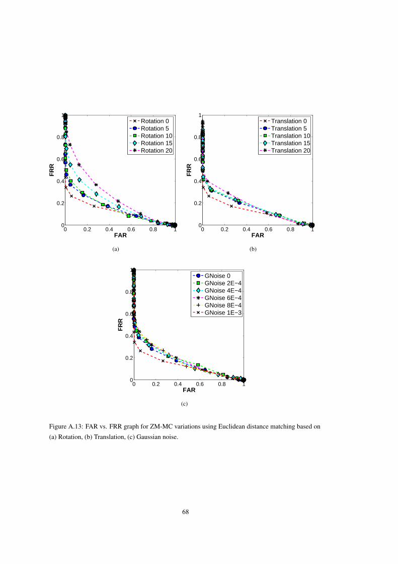
0 0.2 0.4 0.6 0.8 10

0.2

0.4

0.6

0.8

1

FAR

FR

R


(a)

0 0.2 0.4 0.6 0.8 10

0.2

0.4

0.6

0.8

1

FAR

FR

R


(b)

0 0.2 0.4 0.6 0.8 10

0.2

0.4

0.6

0.8

1

FAR

FR

R


(c)

Figure A.13: FAR vs. FRR graph for ZM-MC variations using Euclidean distance matching based on


68

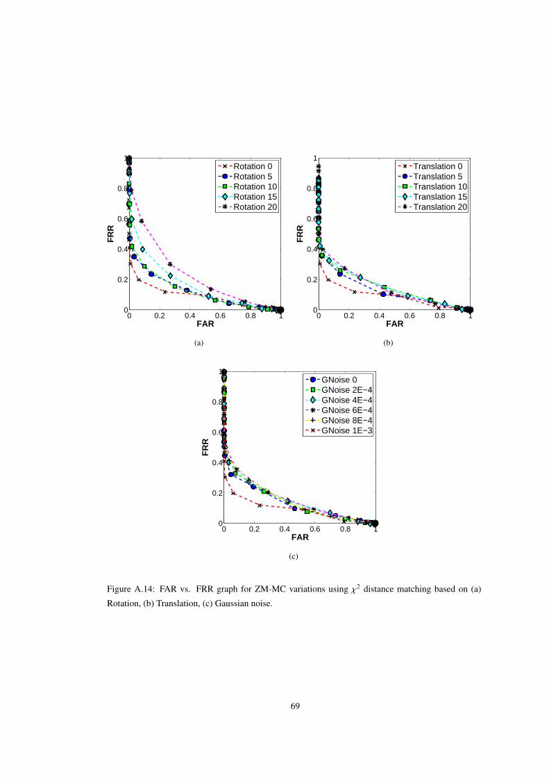
0 0.2 0.4 0.6 0.8 10

0.2

0.4

0.6

0.8

1

FAR

FR

R


(a)

0 0.2 0.4 0.6 0.8 10

0.2

0.4

0.6

0.8

1

FAR

FR

R


(b)

0 0.2 0.4 0.6 0.8 10

0.2

0.4

0.6

0.8

1

FAR

FR

R


(c)

Figure A.14: FAR vs. FRR graph for ZM-MC variations using χ2 distance matching based on (a)


69

0 0.2 0.4 0.6 0.8 10

0.2

0.4

0.6

0.8

1

FAR

FR

R


(a)

0 0.2 0.4 0.6 0.8 10

0.2

0.4

0.6

0.8

1

FAR

FR

R


(b)

0 0.2 0.4 0.6 0.8 10

0.2

0.4

0.6

0.8

1

FAR

FR

R


(c)

Figure A.15: FAR vs. FRR graph for ZM-MC variations using Earth Mover’s distance matching based


70

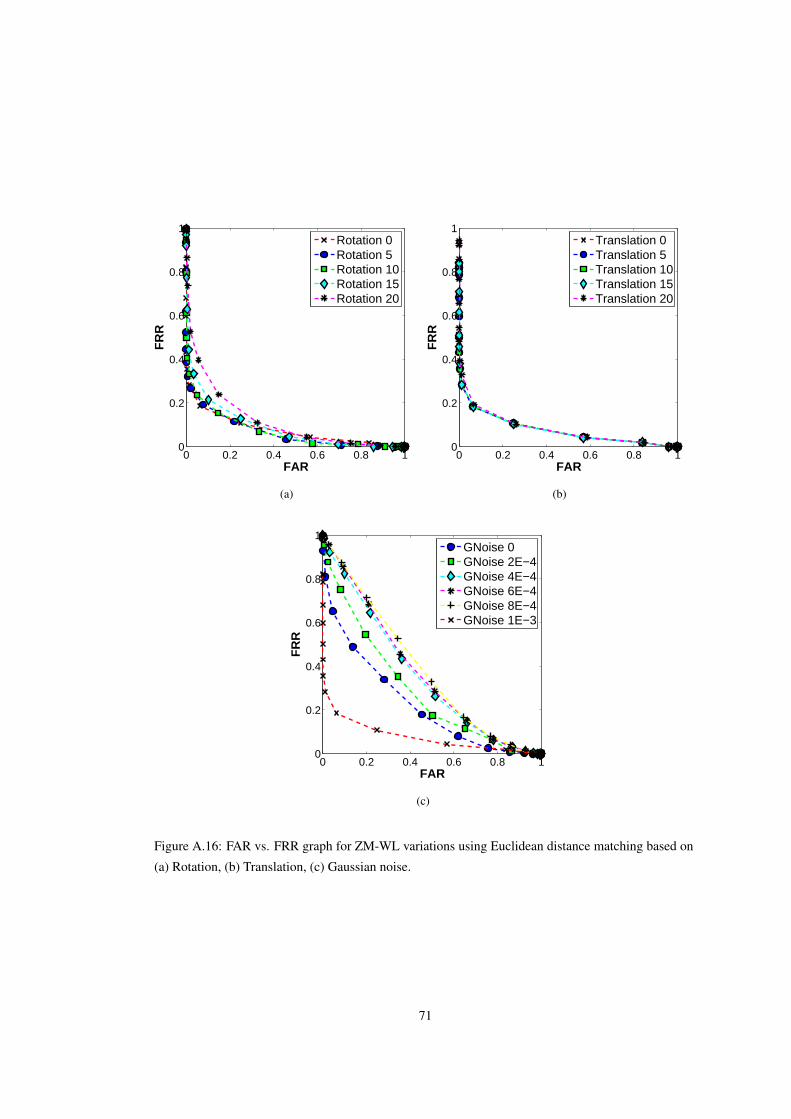
0 0.2 0.4 0.6 0.8 10

0.2

0.4

0.6

0.8

1

FAR

FR

R


(a)

0 0.2 0.4 0.6 0.8 10

0.2

0.4

0.6

0.8

1

FAR

FR

R


(b)

0 0.2 0.4 0.6 0.8 10

0.2

0.4

0.6

0.8

1

FAR

FR

R


(c)

Figure A.16: FAR vs. FRR graph for ZM-WL variations using Euclidean distance matching based on


71

0 0.2 0.4 0.6 0.8 10

0.2

0.4

0.6

0.8

1

FAR

FR

R


(a)

0 0.2 0.4 0.6 0.8 10

0.2

0.4

0.6

0.8

1

FARF

RR


(b)

0 0.2 0.4 0.6 0.8 10

0.2

0.4

0.6

0.8

1

FAR

FR

R


(c)

Figure A.17: FAR vs. FRR graph for ZM-WL variations using χ2 distance matching based on (a)


72

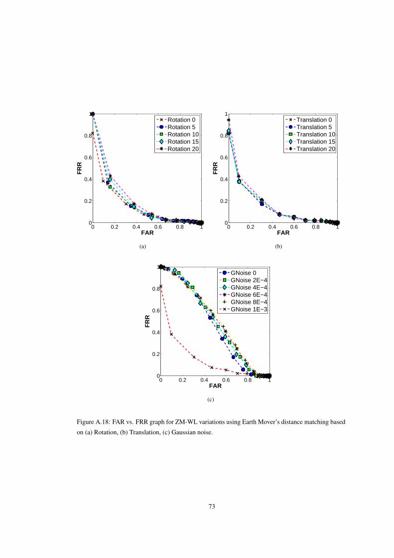
0 0.2 0.4 0.6 0.8 10

0.2

0.4

0.6

0.8

1

FAR

FR

R


(a)

0 0.2 0.4 0.6 0.8 10

0.2

0.4

0.6

0.8

1

FAR

FR

R


(b)

0 0.2 0.4 0.6 0.8 10

0.2

0.4

0.6

0.8

1

FAR

FR

R


(c)

Figure A.18: FAR vs. FRR graph for ZM-WL variations using Earth Mover’s distance matching based


73

0 0.2 0.4 0.6 0.8 10

0.2

0.4

0.6

0.8

1

FAR

FR

R


(a)

0 0.2 0.4 0.6 0.8 10

0.2

0.4

0.6

0.8

1

FAR

FR

R


(b)

0 0.2 0.4 0.6 0.8 10

0.2

0.4

0.6

0.8

1

FAR

FR

R


(c)

Figure A.19: FAR vs. FRR graph for LBP-LT variations using Euclidean distance matching based on


74

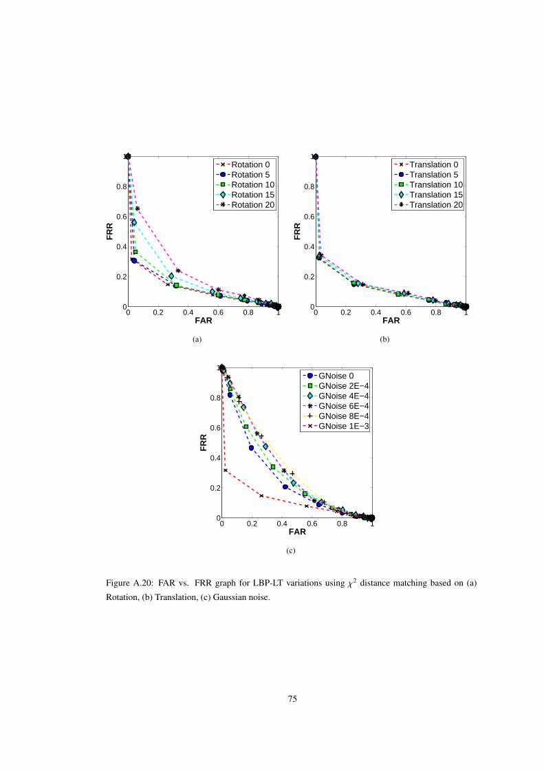
0 0.2 0.4 0.6 0.8 10

0.2

0.4

0.6

0.8

1

FAR

FR

R


(a)

0 0.2 0.4 0.6 0.8 10

0.2

0.4

0.6

0.8

1

FAR

FR

R


(b)

0 0.2 0.4 0.6 0.8 10

0.2

0.4

0.6

0.8

1

FAR

FR

R


(c)

Figure A.20: FAR vs. FRR graph for LBP-LT variations using χ2 distance matching based on (a)


75

0 0.2 0.4 0.6 0.8 10

0.2

0.4

0.6

0.8

1

FAR

FR

R


(a)

0 0.2 0.4 0.6 0.8 10

0.2

0.4

0.6

0.8

1

FAR

FR

R


(b)

0 0.2 0.4 0.6 0.8 10

0.2

0.4

0.6

0.8

1

FAR

FR

R


(c)

Figure A.21: FAR vs. FRR graph for LBP-LT variations using Earth Mover’s distance matching based


76

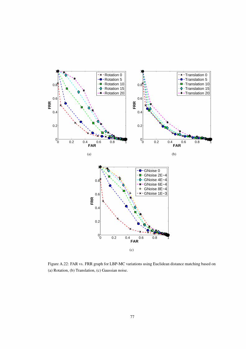
0 0.2 0.4 0.6 0.8 10

0.2

0.4

0.6

0.8

1

FAR

FR

R


(a)

0 0.2 0.4 0.6 0.8 10

0.2

0.4

0.6

0.8

1

FAR

FR

R


(b)

0 0.2 0.4 0.6 0.8 10

0.2

0.4

0.6

0.8

1

FAR

FR

R


(c)

Figure A.22: FAR vs. FRR graph for LBP-MC variations using Euclidean distance matching based on


77

0 0.2 0.4 0.6 0.8 10

0.2

0.4

0.6

0.8

1

FAR

FR

R


(a)

0 0.2 0.4 0.6 0.8 10

0.2

0.4

0.6

0.8

1

FAR

FR

R


(b)

0 0.2 0.4 0.6 0.8 10

0.2

0.4

0.6

0.8

1

FAR

FR

R


(c)

Figure A.23: FAR vs. FRR graph for LBP-MC variations using χ2 distance matching based on (a)


78

0 0.2 0.4 0.6 0.8 10

0.2

0.4

0.6

0.8

1

FAR

FR

R


(a)

0 0.2 0.4 0.6 0.8 10

0.2

0.4

0.6

0.8

1

FAR

FR

R


(b)

0 0.2 0.4 0.6 0.8 10

0.2

0.4

0.6

0.8

1

FAR

FR

R


(c)

Figure A.24: FAR vs. FRR graph for LBP-MC variations using Earth Mover’s distance matching

based on (a) Rotation, (b) Translation, (c) Gaussian noise.

79

0 0.2 0.4 0.6 0.8 10

0.2

0.4

0.6

0.8

1

FAR

FR

R


(a)

0 0.2 0.4 0.6 0.8 10

0.2

0.4

0.6

0.8

1

FAR

FR

R


(b)

0 0.2 0.4 0.6 0.8 10

0.2

0.4

0.6

0.8

1

FAR

FR

R


(c)

Figure A.25: FAR vs. FRR graph for LBP-WL variations using Euclidean distance matching based on


80

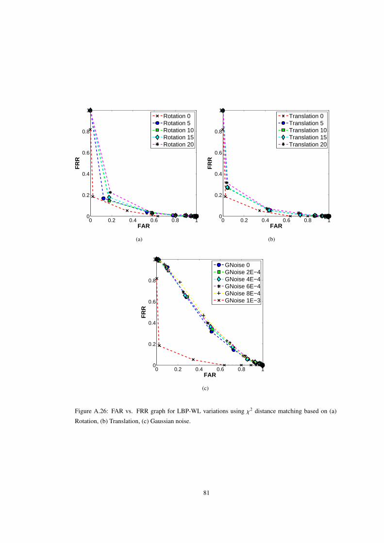
0 0.2 0.4 0.6 0.8 10

0.2

0.4

0.6

0.8

1

FAR

FR

R


(a)

0 0.2 0.4 0.6 0.8 10

0.2

0.4

0.6

0.8

1

FAR

FR

R


(b)

0 0.2 0.4 0.6 0.8 10

0.2

0.4

0.6

0.8

1

FAR

FR

R


(c)

Figure A.26: FAR vs. FRR graph for LBP-WL variations using χ2 distance matching based on (a)


81

0 0.2 0.4 0.6 0.8 10

0.2

0.4

0.6

0.8

1

FAR

FR

R


(a)

0 0.2 0.4 0.6 0.8 10

0.2

0.4

0.6

0.8

1

FAR

FR

R


(b)

0 0.2 0.4 0.6 0.8 10

0.2

0.4

0.6

0.8

1

FAR

FR

R


(c)

Figure A.27: FAR vs. FRR graph for LBP-WL variations using Earth Mover’s distance matching


82

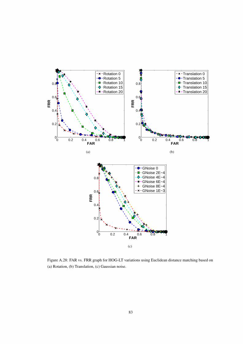
0 0.2 0.4 0.6 0.8 10

0.2

0.4

0.6

0.8

1

FAR

FR

R


(a)

0 0.2 0.4 0.6 0.8 10

0.2

0.4

0.6

0.8

1

FAR

FR

R


(b)

0 0.2 0.4 0.6 0.8 10

0.2

0.4

0.6

0.8

1

FAR

FR

R


(c)

Figure A.28: FAR vs. FRR graph for HOG-LT variations using Euclidean distance matching based on


83

0 0.2 0.4 0.6 0.8 10

0.2

0.4

0.6

0.8

1

FAR

FR

R


(a)

0 0.2 0.4 0.6 0.8 10

0.2

0.4

0.6

0.8

1

FAR

FR

R


(b)

0 0.2 0.4 0.6 0.8 10

0.2

0.4

0.6

0.8

1

FAR

FR

R


(c)

Figure A.29: FAR vs. FRR graph for HOG-LT variations using χ2 distance matching based on (a)


84

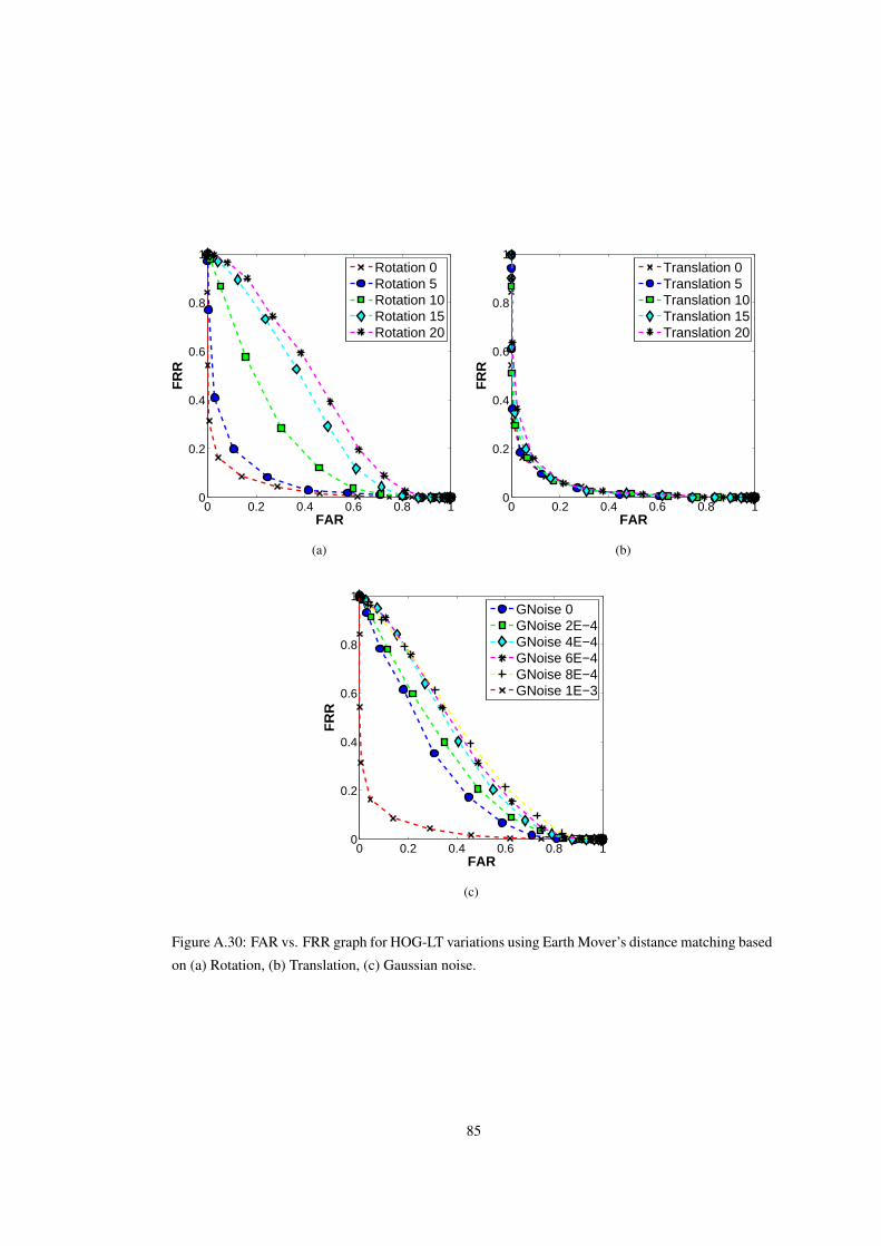
0 0.2 0.4 0.6 0.8 10

0.2

0.4

0.6

0.8

1

FAR

FR

R


(a)

0 0.2 0.4 0.6 0.8 10

0.2

0.4

0.6

0.8

1

FAR

FR

R


(b)

0 0.2 0.4 0.6 0.8 10

0.2

0.4

0.6

0.8

1

FAR

FR

R


(c)

Figure A.30: FAR vs. FRR graph for HOG-LT variations using Earth Mover’s distance matching based


85

0 0.2 0.4 0.6 0.8 10

0.2

0.4

0.6

0.8

1

FAR

FR

R


(a)

0 0.2 0.4 0.6 0.8 10

0.2

0.4

0.6

0.8

1

FAR

FR

R


(b)

0 0.2 0.4 0.6 0.8 10

0.2

0.4

0.6

0.8

1

FAR

FR

R


(c)

Figure A.31: FAR vs. FRR graph for HOG-MC variations using Euclidean distance matching based


86

0 0.2 0.4 0.6 0.8 10

0.2

0.4

0.6

0.8

1

FAR

FR

R


(a)

0 0.2 0.4 0.6 0.8 10

0.2

0.4

0.6

0.8

1

FAR

FR

R


(b)

0 0.2 0.4 0.6 0.8 10

0.2

0.4

0.6

0.8

1

FAR

FR

R


(c)

Figure A.32: FAR vs. FRR graph for HOG-MC variations using χ2 distance matching based on (a)


87

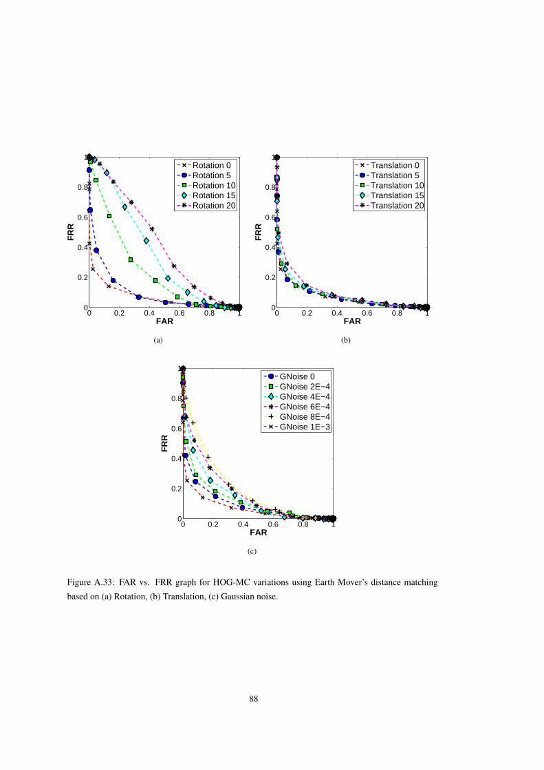
0 0.2 0.4 0.6 0.8 10

0.2

0.4

0.6

0.8

1

FAR

FR

R


(a)

0 0.2 0.4 0.6 0.8 10

0.2

0.4

0.6

0.8

1

FAR

FR

R


(b)

0 0.2 0.4 0.6 0.8 10

0.2

0.4

0.6

0.8

1

FAR

FR

R


(c)

Figure A.33: FAR vs. FRR graph for HOG-MC variations using Earth Mover’s distance matching


88

0 0.2 0.4 0.6 0.8 10

0.2

0.4

0.6

0.8

1

FAR

FR

R


(a)

0 0.2 0.4 0.6 0.8 10

0.2

0.4

0.6

0.8

1

FAR

FR

R


(b)

0 0.2 0.4 0.6 0.8 10

0.2

0.4

0.6

0.8

1

FAR

FR

R


(c)

Figure A.34: FAR vs. FRR graph for HOG-WL variations using Euclidean distance matching based


89

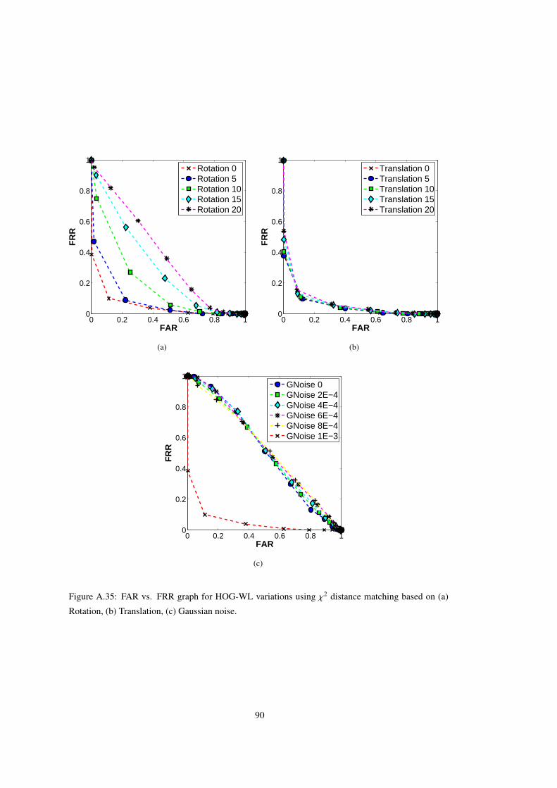
0 0.2 0.4 0.6 0.8 10

0.2

0.4

0.6

0.8

1

FAR

FR

R


(a)

0 0.2 0.4 0.6 0.8 10

0.2

0.4

0.6

0.8

1

FAR

FR

R


(b)

0 0.2 0.4 0.6 0.8 10

0.2

0.4

0.6

0.8

1

FAR

FR

R


(c)

Figure A.35: FAR vs. FRR graph for HOG-WL variations using χ2 distance matching based on (a)


90

0 0.2 0.4 0.6 0.8 10

0.2

0.4

0.6

0.8

1

FAR

FR

R


(a)

0 0.2 0.4 0.6 0.8 10

0.2

0.4

0.6

0.8

1

FAR

FR

R


(b)

0 0.2 0.4 0.6 0.8 10

0.2

0.4

0.6

0.8

1

FAR

FR

R


(c)

Figure A.36: FAR vs. FRR graph for HOG-WL variations using Earth Mover’s distance matching


91

0 0.2 0.4 0.6 0.8 10

0.2

0.4

0.6

0.8

1

FAR

FR

R


(a)

0 0.2 0.4 0.6 0.8 10

0.2

0.4

0.6

0.8

1

FAR

FR

R


(b)

0 0.2 0.4 0.6 0.8 10

0.2

0.4

0.6

0.8

1

FAR

FR

R


(c)

Figure A.37: FAR vs. FRR graph for GBP-LT variations using Euclidean distance matching based on


92

0 0.2 0.4 0.6 0.8 10

0.2

0.4

0.6

0.8

1

FAR

FR

R


(a)

0 0.2 0.4 0.6 0.8 10

0.2

0.4

0.6

0.8

1

FAR

FR

R


(b)

0 0.2 0.4 0.6 0.8 10

0.2

0.4

0.6

0.8

1

FAR

FR

R


(c)

Figure A.38: FAR vs. FRR graph for GBP-LT variations using χ2 distance matching based on (a)


93

0 0.2 0.4 0.6 0.8 10

0.2

0.4

0.6

0.8

1

FAR

FR

R


(a)

0 0.2 0.4 0.6 0.8 10

0.2

0.4

0.6

0.8

1

FAR

FR

R


(b)

0 0.2 0.4 0.6 0.8 10

0.2

0.4

0.6

0.8

1

FAR

FR

R


(c)

Figure A.39: FAR vs. FRR graph for GBP-LT variations using Earth Mover’s distance matching based


94

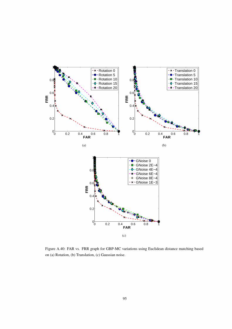
0 0.2 0.4 0.6 0.8 10

0.2

0.4

0.6

0.8

1

FAR

FR

R


(a)

0 0.2 0.4 0.6 0.8 10

0.2

0.4

0.6

0.8

1

FAR

FR

R


(b)

0 0.2 0.4 0.6 0.8 10

0.2

0.4

0.6

0.8

1

FAR

FR

R


(c)

Figure A.40: FAR vs. FRR graph for GBP-MC variations using Euclidean distance matching based


95

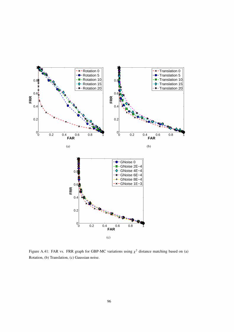
0 0.2 0.4 0.6 0.8 10

0.2

0.4

0.6

0.8

1

FAR

FR

R


(a)

0 0.2 0.4 0.6 0.8 10

0.2

0.4

0.6

0.8

1

FAR

FR

R


(b)

0 0.2 0.4 0.6 0.8 10

0.2

0.4

0.6

0.8

1

FAR

FR

R


(c)

Figure A.41: FAR vs. FRR graph for GBP-MC variations using χ2 distance matching based on (a)


96

0 0.2 0.4 0.6 0.8 10

0.2

0.4

0.6

0.8

1

FAR

FR

R


(a)

0 0.2 0.4 0.6 0.8 10

0.2

0.4

0.6

0.8

1

FAR

FR

R


(b)

0 0.2 0.4 0.6 0.8 10

0.2

0.4

0.6

0.8

1

FAR

FR

R


(c)

Figure A.42: FAR vs. FRR graph for GBP-MC variations using Earth Mover’s distance matching


97

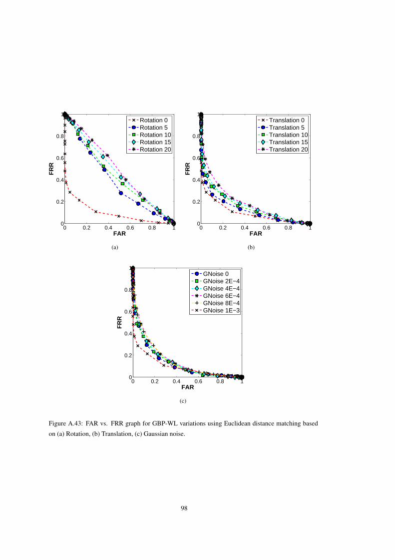
0 0.2 0.4 0.6 0.8 10

0.2

0.4

0.6

0.8

1

FAR

FR

R


(a)

0 0.2 0.4 0.6 0.8 10

0.2

0.4

0.6

0.8

1

FAR

FR

R


(b)

0 0.2 0.4 0.6 0.8 10

0.2

0.4

0.6

0.8

1

FAR

FR

R


(c)

Figure A.43: FAR vs. FRR graph for GBP-WL variations using Euclidean distance matching based


98

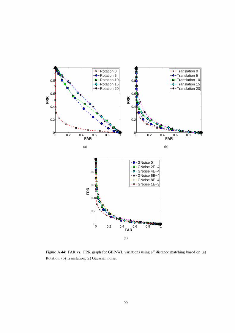
0 0.2 0.4 0.6 0.8 10

0.2

0.4

0.6

0.8

1

FAR

FR

R


(a)

0 0.2 0.4 0.6 0.8 10

0.2

0.4

0.6

0.8

1

FAR

FR

R


(b)

0 0.2 0.4 0.6 0.8 10

0.2

0.4

0.6

0.8

1

FAR

FR

R


(c)

Figure A.44: FAR vs. FRR graph for GBP-WL variations using χ2 distance matching based on (a)


99

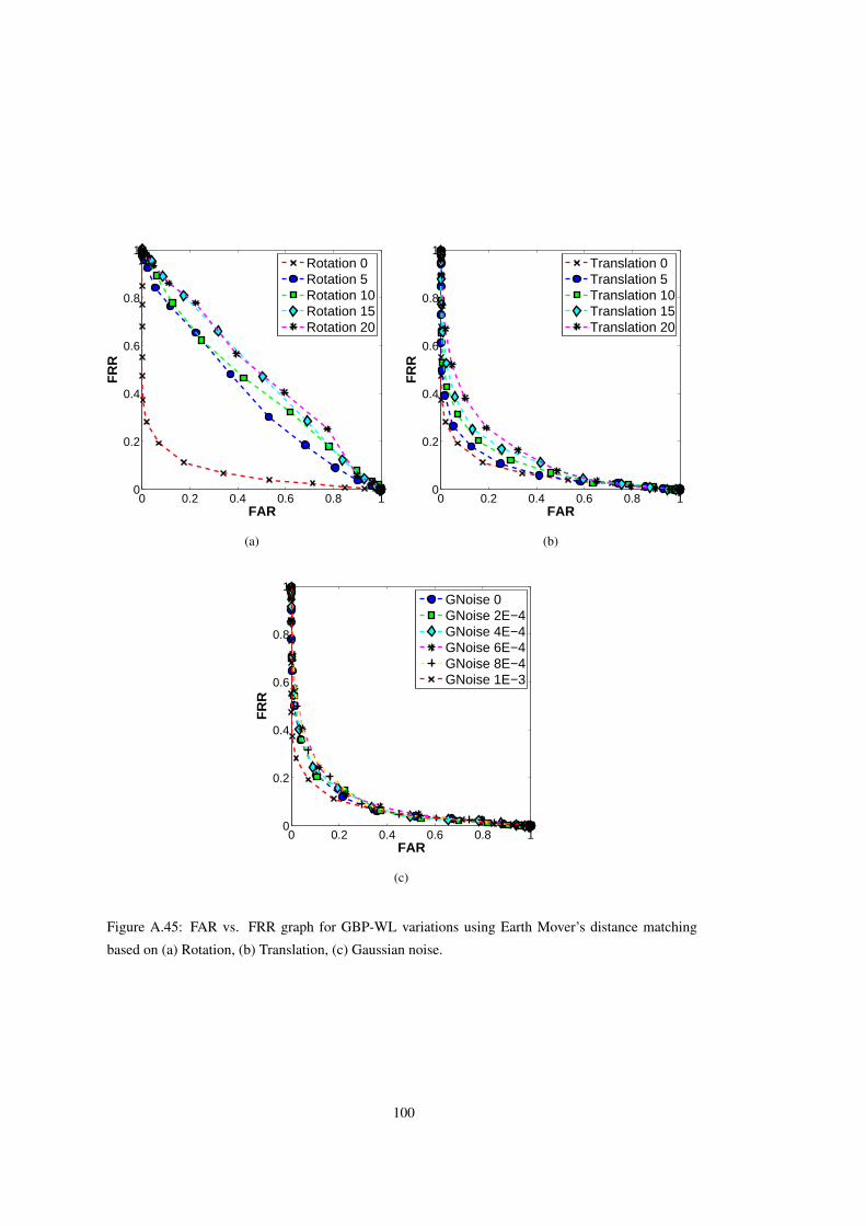
0 0.2 0.4 0.6 0.8 10

0.2

0.4

0.6

0.8

1

FAR

FR

R


(a)

0 0.2 0.4 0.6 0.8 10

0.2

0.4

0.6

0.8

1

FAR

FR

R


(b)

0 0.2 0.4 0.6 0.8 10

0.2

0.4

0.6

0.8

1

FAR

FR

R


(c)

Figure A.45: FAR vs. FRR graph for GBP-WL variations using Earth Mover’s distance matching


100

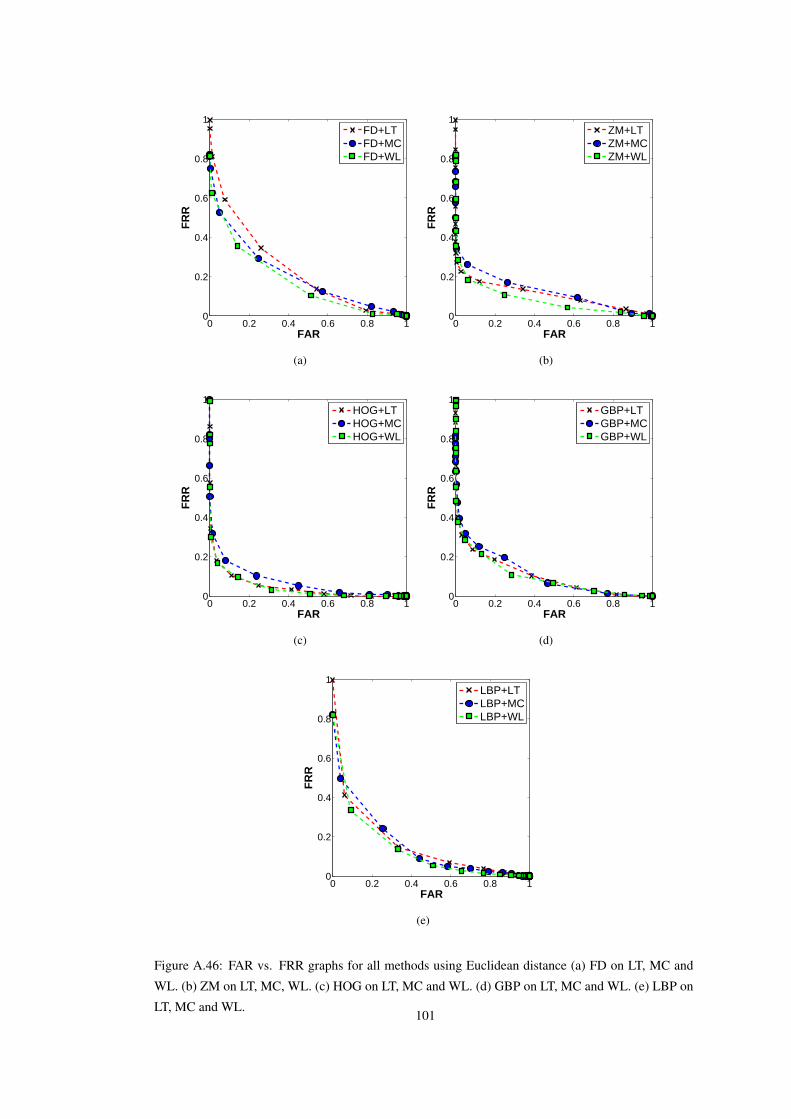
0 0.2 0.4 0.6 0.8 10

0.2

0.4

0.6

0.8

1

FAR

FR

R

FD+LTFD+MCFD+WL

(a)

0 0.2 0.4 0.6 0.8 10

0.2

0.4

0.6

0.8

1

FAR

FR

R

ZM+LTZM+MCZM+WL

(b)

0 0.2 0.4 0.6 0.8 10

0.2

0.4

0.6

0.8

1

FAR

FR

R

HOG+LTHOG+MCHOG+WL

(c)

0 0.2 0.4 0.6 0.8 10

0.2

0.4

0.6

0.8

1

FAR

FR

R

GBP+LTGBP+MCGBP+WL

(d)

0 0.2 0.4 0.6 0.8 10

0.2

0.4

0.6

0.8

1

FAR

FR

R

LBP+LTLBP+MCLBP+WL

(e)

Figure A.46: FAR vs. FRR graphs for all methods using Euclidean distance (a) FD on LT, MC and

WL. (b) ZM on LT, MC, WL. (c) HOG on LT, MC and WL. (d) GBP on LT, MC and WL. (e) LBP on

LT, MC and WL.101

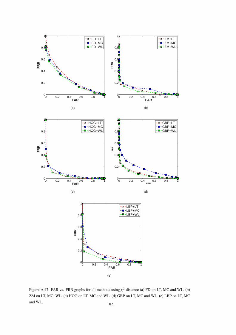
0 0.2 0.4 0.6 0.8 10

0.2

0.4

0.6

0.8

1

FAR

FR

R

FD+LTFD+MCFD+WL

(a)

0 0.2 0.4 0.6 0.8 10

0.2

0.4

0.6

0.8

1

FAR

FR

R

ZM+LTZM+MCZM+WL

(b)

0 0.2 0.4 0.6 0.8 10

0.2

0.4

0.6

0.8

1

FAR

FR

R

HOG+LTHOG+MCHOG+WL

(c)

0 0.2 0.4 0.6 0.8 10

0.2

0.4

0.6

0.8

1

FAR

FR

R

GBP+LTGBP+MCGBP+WL

(d)

0 0.2 0.4 0.6 0.8 10

0.2

0.4

0.6

0.8

1

FAR

FR

R

LBP+LTLBP+MCLBP+WL

(e)

Figure A.47: FAR vs. FRR graphs for all methods using χ2 distance (a) FD on LT, MC and WL. (b)

ZM on LT, MC, WL. (c) HOG on LT, MC and WL. (d) GBP on LT, MC and WL. (e) LBP on LT, MC

and WL. 102

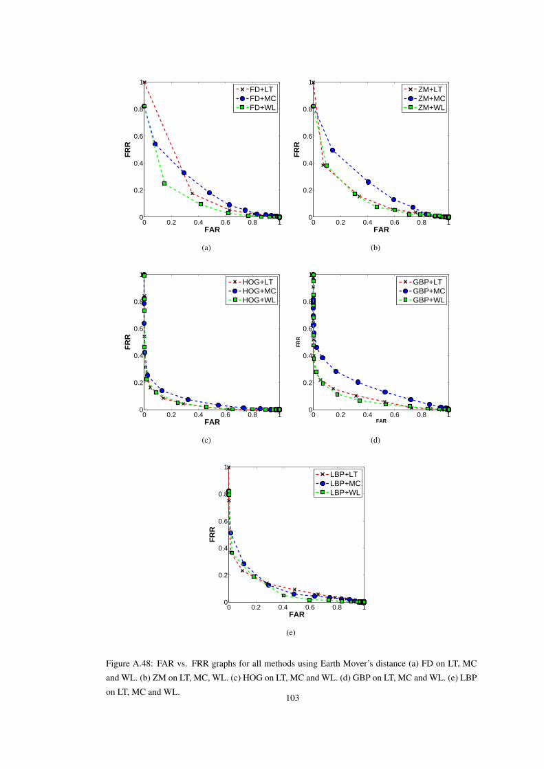
0 0.2 0.4 0.6 0.8 10

0.2

0.4

0.6

0.8

1

FAR

FR

R

FD+LTFD+MCFD+WL

(a)

0 0.2 0.4 0.6 0.8 10

0.2

0.4

0.6

0.8

1

FAR

FR

R

ZM+LTZM+MCZM+WL

(b)

0 0.2 0.4 0.6 0.8 10

0.2

0.4

0.6

0.8

1

FAR

FR

R

HOG+LTHOG+MCHOG+WL

(c)

0 0.2 0.4 0.6 0.8 10

0.2

0.4

0.6

0.8

1

FAR

FR

R

GBP+LTGBP+MCGBP+WL

(d)

0 0.2 0.4 0.6 0.8 10

0.2

0.4

0.6

0.8

1

FAR

FR

R

LBP+LTLBP+MCLBP+WL

(e)

Figure A.48: FAR vs. FRR graphs for all methods using Earth Mover’s distance (a) FD on LT, MC

and WL. (b) ZM on LT, MC, WL. (c) HOG on LT, MC and WL. (d) GBP on LT, MC and WL. (e) LBP

on LT, MC and WL.103

Documents

ANALYSIS OF METHODS FOR FINGER VEIN RECOGNITION A THESIS …