Quality & Quantity30: 405-426, 1996. 405 �9 1996 Kluwer Academic Publishers. Printed in the Netherlands.

Analysis of longitudinal data using the hierarchical l inear model

TOM SNIJDERS University of Groningen, ICS/Department of Statistics and Measurement Theory, Grote Kruisstraat 2/1, 9712 TS Groningen, The Netherlands

Abstract. The hierarchical linear model in a linear model with nested random coefficients, fruitfully used for multilevel research. A tutorial is presented on the use of this model for the analysis of longitudinal data, i.e., repeated data on the same subjects. An important advantage of this approach is that differences across subjects in the numbers and spacings of measurement occasions do not present a problem, and that changing covariates can easily be handled. The tutorial approaches the longitudinal data as measurements on populations of (subject-specific) functions.

Key words. Multilevel analysis, hierarchical linear model, random coefficients.

1. When and why use the hierarchical linear model for analyzing longitudinal data?

A large variety of statistical methods exists for the analysis of longitudinal data. This paper is a tutorial that explains the use of the hierarchical linear model, also referred to as the multilevel model, for analysing longitudinal data. The hierarchical linear model is a random coefficient model with nested random coefficients. As an example a data set is used which was collected by Ormel and coworkers (1991), in a study of the relationship of neuroticism with aging. In this introductory section, the place of random coefficient models as compared to other models is indicated, without presenting an overview of other models. Such overviews may be found, e.g., in Lindsey (1993), Diggle et al. (1994), Dale and Davies (1994).

The type of data under consideration is data about a sample of individuals, for each of whom values on an array of variables are recorded at several points in time. For the individuals I think primarily of persons, but one could also think of other units such as companies, municipalities, countries, etc. Instead of time there might be a different ordering principle. E.g., the measurements might refer to individuals under each of several experimental conditions. Depending on the research question, the time dimension can be age, but also calendar year and date, time elapsed since the onset of

406 T. Sni jders

psychotherapy or since a relevant life event, etc. Symbolically, the data can be represented as

Y~(t),&,(t),. . . . . Xqi(t) for t �9 ~ - (1)

z l i . . . . . z~i (2)

where

- i is the index number of the individual; - Y is the variable treated as the d ep en d en t variable; - xl to Xq and zl to zr are variables treated as the exp lanatory , or indepen-

dent, variables; the Xk are called changing , and the zk cons tant covariates; - t is the time of measurement, and ~ is the set of time points at which

measurements Yi ( t ) , Xli ( t ) , . . . , Xqi (t) for individual i are available.

The numbers, q and r, of changing and constant covariates, may be zero or positive. In the extreme case where q - - r - - 0 , there are no explanatory variables at all. As the notation ~- indicates, the measurement occasions may differ between individuals; also the numbers of measurements may differ between individuals. (In spite of the longitudinal aspects, it is even permitted that for some individuals only one measurement is available.) The number of measurements for individual i, i.e., the cardinality of ~ , is denoted ni. It is assumed that the individual-specific number and spacing of observation do not carry any relevant information, but that they may be treated as being determined by the researcher (and by chance, as in the case of failing apparatus that causes the omission of some measurements). This excludes, e.g., event history data.

The methods presented in this paper are designed for the situation, where one wishes to investigate the effects on Y of time and the explanatory variables x1 to Xq and zl to Zr. AS such, these methods can be seen as generalisations of multiple regression analysis and of analysis of variance and covariance. We focus on dependent variables Y that have an interval level of measurement, i.e., the interpretation of how important the difference is between values Y0 and Y0 + 2~y depends on how large Ay is, but not on the 'reference value' Y0. This corresponds to the assumption, made below, that 'residuals', or 'non-explained parts' of Y, are assumed to be normally distributed. This excludes dichotomous and other categorical variables. Ex- tensions of the methods presented are available for dichotomous and some other types of dependent variable, but they will not be specifically treated below.

The type of random coefficient model treated in this paper is the Hierarch-

Analysis of longitudinal data 407

ical Linear Model (HLM) that has been used so fruitfully in multilevel analysis (Goldstein (1987), Bryk and Raudenbush (1992)). This implies that the random coefficients are hierarchically nested in some meaningful way. The nesting levels are usually numbered: the lowest, most detailed level is called the first, etc., so that we speak of level-1 units nested within level-2 units nested within level-3 units, etc. In most applications, there are 2 levels of nesting; data with 3 nesting levels occur occasionally, but data structures with more than 3 nesting levels are rare. The paradigmatic situation for multilevel analysis is individuals nested in groups: e.g., pupils nested in school classes, employees nested in companies, persons nested in peer groups. Level 1 then corresponds to individuals, level 2 to groups. For longitudinal data, the nesting structure is measurements nested in individuals. Now the indivi- duals are the units at level 2, and the time points, or measurements, are the units at level 1.

The use of the HLM for longitudinal data has been discussed in many publications: e.g., Rogosa et al. (1982) (restricting attention to linear curves); Laird and Ware (1982); Sternio et al. (1983); Rogosa and Willett (1985); Goldstein (1987, ch. 4); Goldstein (1989); Bryk and Raudenbush (1987 and 1992, ch. 6); Alsaker (1992); Hoeksma and Koomen (1992); Raudenbush and Chan (1994); Plewis (1994); Rutter and Elashoff (1994). The random effects models for panel data treated by Swamy (1974), Hsiao (1986), and Kmenta (1986) are related but less flexible for the type of data treated in this paper, because they do not allow for random coefficients in unbalanced designs; some of the models presented by Kmenta (1986) are more flexible in other ways, by allowing certain forms of autocorrelation and crossed random effects. For fixed occasion designs, where all subjects provide mea- surements on the same set of occasions and where there are no missing data, and provided that the explanatory variables (the x- and z-variables) have multivariate normal distributions, these models can also be formulated as covariance structure ( "LISREL") models. (See Willett and Sayer (1994).)

Some examples of longitudinal data that can be in the format (1), notably of the dependent variables Y, are the following:

- measures of physical or psychological development of children taken at several moments in their youth;

- measures of psychological health of persons taken during a period in their lifetime, or during and after a period of psychotherapy;

- physiological measurements of persons taken at several times during one day;

- income, or attitude measurements of individuals taken over a period of several years;

408 T. Snijders

- unemployment figures in municipalities over a number of years.

In which situations would it be sensible for a researcher to apply the HLM for analysing longitudinal data (assuming that they have the format (1))? The following considerations can be important.

1. When the numbers of measurements, ni, differ across individuals (due to design or to missing data), there are usually no other methods of statistical analysis available that do not throw away part of the data or resort to filling in (imputing) the unknown values. Also when the time points t in

differ across individuals (e.g., children measured at various and differ- ent ages) and even when the time points are identical across individuals but not equispaced, there may not be a viable alternative to the HLM.

As a particular case, when the data are repeated measurements at fixed occasions (such as occur frequently, e.g., in psychological experiments) but some of the data are missing, the HLM can be used for a multivariate analysis of variance that uses all available data. (See Maas and Snijders (1995).)

2. The HLM incorporates not only random effects, like the more well-known variance component and panel data models (e.g., Hsiao, 1986), but also random coefficients. In other words, the effects of time and of other changing covariates may differ across individuals.

3. It is straightforward to incorporate not only covariates zk that are constant in time, but also changing covariates x~(t).

4. With the use of the HLM it is natural to focus the analysis on the development curves of the individuals, not only on their average level but also on the speed or acceleration of development, or on other characteris- tics of the way in which Y changes with time. Focusing on individual growth curves was proposed by Rogosa et al. (1982) and by Rogosa and Willett (1985). It is possible with the HLM to answer many relevant questions, such as about which differences exist between individuals with respect to their development curves, and which covariates have effects on the level, speed, and 'shape' of development.

5. The HLM can be applied also when the number of measurements per individual, nl, is large compared to the number of individuals. Methods such as multivariate analysis of variance for repeated measurements can- not fruitfully be used in such situations, because too many parameters will need to be fitted to the covariance matrix.

6. If there are more nesting levels in the data, these can be easily represented in the model by using a 3-(or more) level-model. Two general examples

Analysis of longitudinal data 409

are longitudinal data on individuals in groups (groups constitute the third level), and data collected at several moments in time during several days (time is the first level, day the second, individual the third). A specific example is a car driving experiment where subjects repeatedly drove a certain road under different instructions, and where speed was measured in all bends of the road (bend is the first level, ride the second, subject the third).

Several computer programs have been developed for statistical data analysis on the basis of the HLM: one program itself called HLM (Bryk et al., 1994), ML3 (Prosser et al., 1991), and VARCL (Longford, 1993).

In practice, data sets are complicated and there does not exist one single preferred approach to arrive at a statistical model. In the multilevel model, explanatory variables can have fixed effects but also random effects, which makes model selection even more complicated than it already is for the more usual regression models.

If there are theoretical considerations which can serve as a guide during the model selection process, then these should be used as much as possible. In the example presented in this paper, however, the use of such theoretical considerations is very limited. The approach followed in this paper is a forward selection approach: the start is an empty model, and the model is made more and more complicated. In particular, changing covariates are included at the end of the model selection process. This is not necessary the best approach to follow, as will be mentioned in the section on covariates and in the discussion.

2. Populations of curves

The HLM for longitudinal data can be formulated as a model for apopulation o f curves. This section indicates how such a population of curves can be modeled without using covariates. In the next section, the use of time- depending and constant covariates will be discussed.

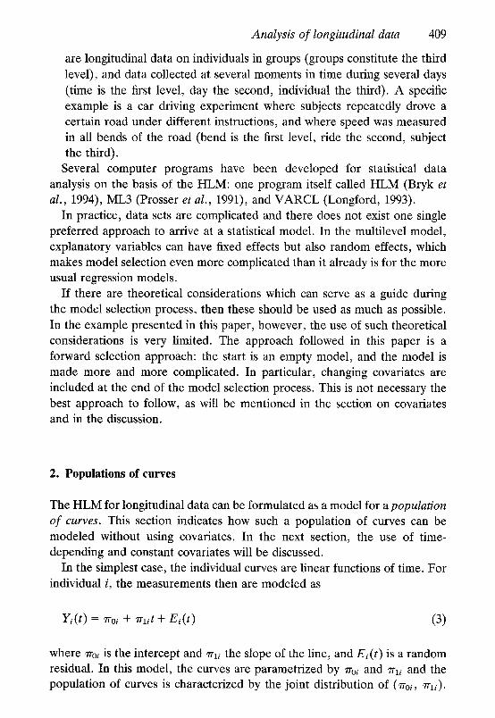
In the simplest case, the individual curves are linear functions of time. For individual i, the measurements then are modeled as

Yi(t) = 7roi + ~rut + El(t) (3)

where ~'oi is the intercept and ~'1i the slope of the line, and Ei(t) is a random residual. In this model, the curves are parametrized by ~'o~ and zrli and the population of curves is characterized by the joint distribution of (~roi, ~'1i).

410 T. Snijders

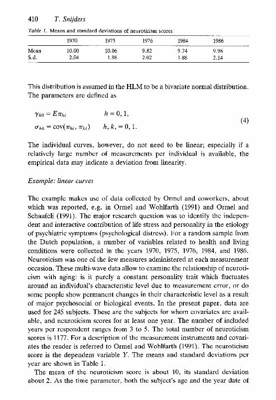
Table i. Means and standard deviations of neuroticism scores

1970 1975 1976 1984 1986

Mean 10.00 10.06 9.82 9.74 9.98 S.d. 2.04 1.98 2.02 1.88 2.14

This distribution is assumed in the H L M to be a bivariate normal distribution. The parameters are defined as

Tho = E'rghi h = O, 1, (4)

~rhk = COV(~'m, ~'ki) h, k, = 0, 1.

The individual curves, however, do not need to be linear; especially if a relatively large number of measurements per individual is available, the empirical data may indicate a deviation from linearity.

Example: linear curves

The example makes use of data collected by Ormel and coworkers, about which was reported, e.g. in Ormel and Wohlfarth (1991) and Ormel and Schaufeli (1991). The major research question was to identify the indepen- dent and interactive contribution of life stress and personality in the etiology of psychiatric symptoms (psychological distress). For a random sample from the Dutch population, a number of variables related to health and living conditions were collected in the years 1970, 1975, 1976, 1984, and 1986. Neuroticism was one of the few measures administered at each measurement occasion. These multi-wave data allow to examine the relationship of neuroti- cism with aging: is it purely a constant personality trait which fluctuates around an individual's characteristic level due to measurement error, or do

some people show permanent changes in their characteristic level as a result of major psychosocial or biological events. In the present paper, data are used for 245 subjects. These are the subjects for whom covariates are avail- able, and neuroticism scores for at least one year. The number of included years per respondent ranges from 3 to 5. The total number of neuroticism scores is 1177. For a description of the measurement instruments and covari- ates the reader is referred to Ormel and Wohlfarth (1991). The neuroticism score is the dependent variable Y. The means and standard deviations per year are shown in Table 1.

The mean of the neuroticism score is about 10, its standard deviation about 2. As the time parameter, both the subject's age and the year date of

Analysis of longitudinal data

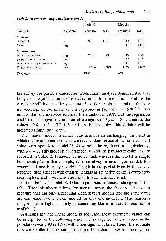
Table 2. Neuroticism: empty and linear models

411

Model 0 Model 1

Parameter Variable Estimate S.E. Estimate S.E.

Fixed part Intercept 7oo Year 3'1o

Random part Intercept variance ~roo Slope variance: year ~rll Intercept - slope covariance ~rol Residual variance o "2

Deviance

9.91 0.10 9.90 0.10 -0.075 0.081

2.31 0.24 2.36 0.24 0.79 0.15

-0.01 0.13 1.584 0.073 1.25 0.067

4390.2 4338.1

the survey are possible candidates. Preliminary analyses demonstrated that the year date yields a more satisfactory model for these data. Therefore the variable t will indicate the year date. In order to obtain numbers that are not too large or too small, year is expressed as (year date - 1978)/10. This implies that the intercept refers to the situation in 1978, and the regression coefficient on t gives the amount of change per 10 years. So t assumes the values -0.8, -0.3, -0.2, 0.6, and 0.8. In the tables, this variable will be indicated simply by "year".

The "naive" model in which neuroticism is an unchanging trait, and in which the several measurements are independent retests of the same constant value, corresponds to model (3, 4) without the ~1i term or, equivalently, w i t h o'11 = 0. This model is called model 0, and the parameter estimates are reported in Table 2. It should be noted that, whereas this model is simple but meaningful in this example, it is not always a meaningful model. For example, if one is analyzing child length in the period from birth to ado- lescence, then a model with constant lengths as a function of age is completely meaningless, and I would not advise to fit such a model at all.

Fitting the linear model (3, 4) led to parameter estimates also given in this table. The table also mentions, for later reference, the deviance. This is a fit measure that has only a meaning when several models (for the same data) are compared, not when considered for only one model fit. (The reason is that, unlike in loglinear analysis, something like a saturated model is not available.)

Assuming that the linear model is adequate, these parameter values can be interpreted in the following way. The average neuroticism score in the population was 9.90 in 1978, with a non-significant linear trend (the estimate of 3'1o is smaller than its standard error). Individual curves for the develop-

412 T. Sn i jders

ment of neuroticism vary around this mean population curve. The standard deviation of individual values around this curve in 1978 is ~ = 1.54, and the individual curves have slopes with a standard deviation of ~ = 0.89 points per 10 year. An individual with a high positive slope, e.g., will have

a slope ~'1i of about E~li + 2 S.D.(r = 3'10 + 2 ~ = 1.7 points per 10 year. Over a period of 10 years this is a considerable amount given the over- all standard deviation of almost 2. The correlation between the individual's trend value in 1978, and his slope, is negligible: p(Tr0i,Trli) = - 0 . 0 1 N 2 . 3 6 • 0.79 = 0.007. Finally, the deviation of the score around the trend value, which includes its measurement error, has a standard deviation of ~ = 1.12.

Below we indicate how the significance of the various model parameters can be tested. Running ahead, we mention already now that a test for the

significance of the slope variance, o-~1, yields a chi-squared value of 51.9 at 2 degrees of freedom, an extremely significant result. Thia implies that model 1 gives a much better fit than the model that has only a fixed, and not a

random, effect of year.

2.1. N o n - l i n e a r curves

A more general formulation than (3) is based on suitable functions of time, denoted f h ( t ) and numbered h = 0 . . . . . p. (Often, but not always, f o ( t ) will be the constant f o ( t ) - 1.) Sometimes, a convenient family of functions is the family o f p o l y n o m i a l s , f h ( t ) = t h. Representat ion (3) then is extended to

Y i ( t ) = 1roi + 7flit + Ir2it 2 + �9 �9 �9 + "h'pi tp + E i ( t ) . (5)

The number p is then called the degree of the polynomial. E.g., when using polynomials, linearity of the individual development functions can be tested by testing the null hypothesis "p = 1" against the alternative hypothesis of a quadratic relation, "p = 2". Note that any function of which the value is known for m points can be represented exactly by a polynomial of degree m - 1. Hence, if all individuals are measured at the same m time points, it makes no sense to use polynomials of degree more than m - 1 (and from a statistical point of view, it will usually be bet ter to use a degree considerably lower than m - 1). Polynomials are not always the best choice, however, and the use of splines is another possibility (not discussed here for lack of space). In the specific case of circadian or other periodic rhythms, it can be useful to work with trigonometric functions. If the functions are not necessar- ily polynomials but are denoted more generally by f h ( t ) , we obtain the representation

Analysis of longitudinal data 413

Yi(t) = 7roifo(t) + 7rlifl(t) + 7r2if2(t) + " " + 7rpifp(t) + Ei(t) p

E ~hifh(t) + El(t). (6 ) h=O

The further modeling a population of curves (6) is based on the following

two ideas:

- The individual-specific parameters (Tr0i, �9 �9 7rpi) are regarded as stochas- tic coefficients, and their joint distribution is modeled by a multivariate normal distribution.

- There usually are some functions fh(t) , for which the available data do not provide evidence that their coefficients 7rh~ are indeed individual- specific; the latter coefficients may also have the same value for all indivi- duals. Thus, the variability across individuals is tested for the parameters ~'h~; those that do not exhibit significant variability are modeled as con- stants.

Combining these two ideas means that some of the parameters 7rh~ vary stochastically over the population, others are fixed. When working with polynomials, it will be natural that the coefficients of the lower order terms t h a r e individual-specific, whereas those of the higher order terms are

constant. Also when working with other families of functions, it is often natural to let the coefficients of the first functions fh(t) be individual-specific and those of the last be constant. This leads to the following formulation,

where the number of individual-specific coefficients is denoted P0, with

0 ~<P0 ~<P:

1rhi = 7ho + Uhi for h = 0 . . . . . Po; (7)

1rm = YhO for h =Po + 1 , . . . ,p.

The reason for the extra subscript 0 for the 3' parameters will become clear below.

For h ~< p0, the YhO parameter is the mean value of the individual-specific coefficients ~'hi ; for h > Po, YhO is the constant value of 7rh/for all individuals i. The YhO parameters are referred to as fixed coefficients, or regression coefficients. The terms Uhi = 7 r h i - - YhO are the individual deviations from these mean values. The following assumption is made with regard to these deviations:

414 T. Snijders

�9 The vector (Uol . . . . . Upoi ) has a multivariate normal distribution, with mean 0 and covariance matrix E.

Thus, the parameters of the statistical model for this population of curves

are the p fixed coefficients yho, the Po x Po covariance matrix E = (O'hk), and the residual variance (r 2 e - - var(Ei (t)). The variances O'hh will also be denoted by o ~2. These parameters can be interpreted as follows: the model is characterized by the population mean curve, given by

E(Yi(t)) = Yoofo(t) + ylofl(t) + " " + 7pofp(t), (8)

by the individual deviations from this curve of which the coefficients have a multivariate normal distribution with mean 0 and covariance matrix E, and by

the residuals (sometimes interpretable as measurement errors) with variance ~r 2 .

Example: non-linear curves

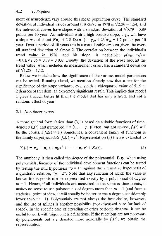
As a first step ("model 2"), we fit the mean curve exactly. Since there are 5 time points, this can be done by using a 4th degree polynomial. An equivalent approach is to use dummy variables. We choose the latter option,

because the coefficients of the dummy variables are more easily interpretable than the coefficients of high degree polynomials. It should be kept in mind that whether one uses 4 dummy variables or a 4th degree polynomial is just

a matter of parametrisation, and not a difference between two statistical models. The first year, 1970, is used as the reference category, and separate dummy variables for each of the years 1975 to 1986 are used in the fixed

part of the model. Subsequently, a model (number 3) is fitted where the individual deviations from the average curve follow a quadratic trend. Results from these two models are presented in Table 3. Whether the improvements

of models 2 and 3 over the linear model presented in Table 2 are significant, is discussed below.

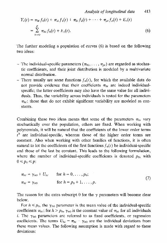
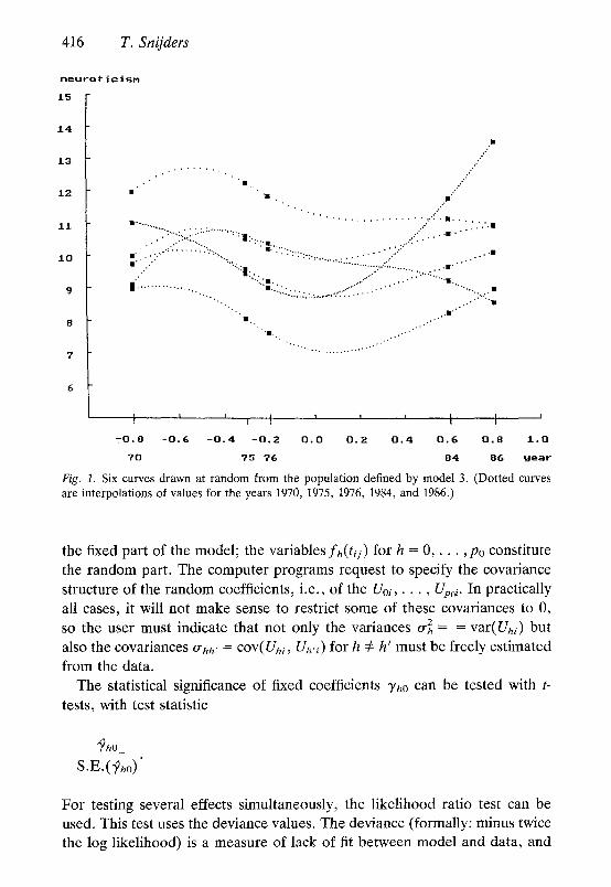
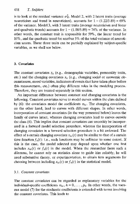
In Figure 1, six curves are presented that are drawn at random from the distribution of curves defined by model 3 (estimates in Table 3), with the residual Ei(t) set to 0. Since the data are restricted to the five years of observations (1970-1986), only the values at these years are meaningful. The dotted curves in between are based on interpolation by quadratic splines of the population mean curve for the five years. Since the points in between do not correspond to moments of observations, this interpolation is only for the purpose of obtaining a smooth graph.

Analysis of longitudinal data

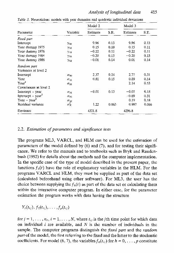
Table 3. Neuroticism: models with year dummies and quadratic individual deviations

415

Model 2 Model 3

Parameter Variable Estimate S.E. Estimate S.E.

Fixed part Intercept 700 9.96 0.13 Year dummy 1975 730 0.15 0.10 Year dummy 1976 3'4o -0.22 0.11 Year dummy 1984 Yso -0.20 0.13 Year dummy 1986 3̀ 60 -0.01 0.14

Random part Variances at level 2 Intercept 0"00 2,37 0.24 Year 0"11 0,81 0.15 Year 2 0-22 Covariances at level 2 Intercept - year 0-01 -0.01 0.13 Intercept - year 2 0-02 Year - year 2 0-12 Residual variance 0-~ 1.22 0.065

Deviance 4321.8

9.96 0.13 0.15 0.11

-0.22 0.11 -0.20 0.13

0.01 0.14

2.77 0.31 0.89 0.14 2.14 0.53

-0.07 0.15 -0.89 0.31

0.19 0.18 0.997 0.066

4296.8

2.2. Estimation of parameters and significance tests

The programs ML3, VARCL, and HLM can be used for the estimation of parameters of the model defined by (6) and (7), and for testing their signifi- cance. We refer to the manuals and to textbooks such as Bryk and Rauden- bush (1992) for details about the methods and the computer implementation. In the specific case of the type of model described in the present paper, the functions fh(t) have the role of explanatory variables in the HLM. For the programs VARCL and HLM, they must be supplied as part of the data set (calculated beforehand using other software). For ML3, the user has the choice between supplying the fh(t) as part of the data set or calculating them within the interactive computer program. In either case, for the parameter estimation the program works with data having the structure

Yi(tij), f t ( t , j ) , . . . , fp(tij)

for j = 1 , . . . , nl, i = 1 . . . . , N, where tii is the j th time point for which data on individual i are available, and N is the number of individuals in the sample. The computer programs distinguish the fixed part and the random part of the model, the first referring to the fixed and the latter to the stochastic coefficients. For model (6, 7), the variables f h ( t i j ) for h = 0 . . . . . p constitute

416 T. Snijders

n e u r o t i e i s n

IS

14

13

12

11

10

9

8

7

6

. l a

�9 �9 , " �9 �9 , ,

I . , . , "

I , III

�9 . . . . , , . - ' "

, , , , , , . . . . . . . . . �9 =-�9 - m , . , ~ . . . . m � 9

...... ?':'"":..i,:':': ......... "=':'l . . . . . . "". � 9 �9 . . . . . , . : ' . . . . . . . . . . . i s . . . . . . , , ' . . " �9

�9 . , . � 9 ' - - v . . - - , , � 9 . . . . . - �9 �9 , , , '

"" . ' " ' . . . . . . . . : i t.. .................. ..:.;=~:- ........... :...;'" �9 . . . . ' �9 ' " . , 'a l , ."" , " " � 9 1 4 9 1 4 9

l . . . . . . . . . . . . . . . . . "=...:. . . . . . . . . . . . . . . . . . . . . . . . . . . . �9 ' �9 ' � 9 ............ " . . . . . . . . , . , ' " " '11

�9 , . - '

�9 , . . . . . , . ' "

" - , � 9 . . . . . . . . , , . ' "

I ' i I ' ' ' I I '

- 0 , 8 - 0 . 6 - 0 , 4 - 0 . 2 0 , 0 0 . 2 0 . 4 0 , 6 0 . 8 1 . 0

70 75 76 84 86 year

Fig. 1. Six curves drawn at random from the population defined by model 3. (Dotted curves are interpolations of values for the years 1970, 1975, 1976, 1984, and 1986.)

the fixed part of the model; the variables fh(t iy) for h = 0 . . . . , po constitute the random part. The computer programs request to specify the covariance

structure of the random coefficients, i.e., of the Uoi . . . . . Upo i. In practically all cases, it will not make sense to restrict some of these covariances to 0, so the user must indicate that not only the variances o-] = = var(Um) but also the covariances o'hh' = cov(Um, Uh,i) for h 4: h' must be freely estimated

from the data. The statistical significance of fixed coefficients %0 can be tested with t -

t e s t s , with test statistic

~?ho S.E.(~o)

For testing several effects simultaneously, the likelihood ratio test can be used. This test uses the deviance values. The deviance (formally: minus twice the log likelihood) is a measure of lack of fit between model and data, and

Analysis of longitudinal data 417

can be calculated with each model fit. The difference between two model fits can be tested with the difference in deviances as test statistic. The null distribution is X 2 and the degrees of freedom are given by the difference in number of parameters. For example, to test the difference between the purely linear model I and model 2, where the mean population curve is fitted exactly, the test statistic obtained is 4338.1 - 4321.8 = 16.3 on 3 degrees of freedom, with a p-value of about 0.001. (This shows that only looking at t- values can be misleading: each of the year dummies in model 2 is not or barely significant, given that the other year dummies are included in the model; but taken together, the year dummies are strongly significant.)

To test the significance of the last included random effect, that of Upoi, is 2 = 0. This can be done in tantamount to testing the null hypothesis Ho : O'po

several ways; a convenient method is again to use the likelihood ratio test, 2 = 0 , the full with the deviance difference as the test statistic. To test Ho : ~rpo

model (with the P0 random effects) must be estimated, yielding a deviance dl, and the restricted model corresponding to the null hypothesis, with Po - 1 random effects, must also be estimated, yielding a deviance do. (Both models must have the same fixed part.) The restricted model has Po + 1 parameters less than the full model (one variance parameter, O'20PO a n d Po covariance parameters ~rhpo, h = 0 , . . . , Po - 1). Because of this, the null hypothesis can be tested with the deviance difference do - dl as the test statistic, having the chi-squared distribution with Po degrees of freedom when the null hypothesis is true: e.g., to test the difference between models 2 and 3 in Table 2, the X 2 value obtained is 4321.8 - 4296.8 = 25.0. A glance at Table 2 shows that model 3 has 3 parameters more than model 2, corresponding to the po + 1 = 3 degrees of freedom. This implies that the random effect of year 2 is strongly significant.

One may wonder, of course, whether a quadratic individual deviation from the mean population curve is sufficient. In this case, with 5 measurement points, a saturated, or fully multivariate, model for the covariance matrix is obtained by using polynomials of degrees up to 4 and giving these random effects at level 2, while deleting the random residual at level 1 (cf. Maas and Snijders, 1995). The resulting decrease in deviance is 6.6 on 8 degrees of freedom. This is far from significant. It can be concluded that, for these data, a model with an arbitrary mean population curve and quadratic individual deviations from the mean curve gives an adequate representation of the data (as long as covariates are not considered).

How far have we come now, without taking covariates into account? The total variance of neuroticism in model 0 is 2.31 + 1.58 = 3.89. Of this vari- ance, a constant latent trait "neuroticism" accounts for 2.31/3.89 = 59%. For calculating the explained variance by models 1 through 3, the easiest thing

418 T. Snijders

is to look at the residual variance o'~. Model 2, with 2 latent traits (average neuroticism and trend in neuroticism), accounts for 1 - (1.22/3.89) = 69% of the variance. Model 3, with 3 latent traits (average neuroticism and linear and quadratic trends) accounts for 1 - (1.00/3.89) = 74% of the variance. In other words, the constant trait is responsible for 59%, the linear trend for 10%, and the quadratic trend for another 5% of the total variance of neuroti- cism scores. These three traits can be partially explained by subject-specific variables, as we shall see below.

3. Covariates

The constant covariates Zk (e.g., demographic variables, personality traits, etc.) and the changing covariates xk (e.g., changing social or economic cir- cumstances, mood variables, indicators of events that have taken place before this measurement, etc.) often play different roles in the modeling process. Therefore, they are treated separately in this section.

An important difference between constant and changing covariates is the following. Constant covariates serve to model curves within the class defined by (6): the covariates model the coefficients ~'ni. The changing covariates, on the other hand, lead to curves with different shapes. In other words, incorporation of constant covariates (in the way presented below) leaves the family of curves intact, whereas changing covariates lead to curves outside the class (6). This implies that constant covariates can smoothly be incorpor- ated in a forward model selection procedure, whereas the incorporation of changing covariates in a forward selection procedure is a bit awkward. The effect of a certain changing covariate xki (t) may be similar to that of a certain time function fh(t): i.e., such functions may be collinear to some extent. If this is the case, the model selected may depend upon whether one first includes xki(t) or fh(t) in the model. When the researcher faces such a dilemma, he cannot rely on statistics alone to guide him reliably; he will need substantive theory, or experimentation, to obtain firm arguments for choosing between including xki(t) or fh(t) in the statistical model.

3.1. Constant covariates

The constant covariates can be regarded as explanatory variables for the individual-specific coefficients ~'ng, h = 0 . . . . , Po. In other words, the vacu- ous model (7) for the stochastic coefficients is extended with terms involving the constant covariates. This leads to

Analys is o f longitudinal data 419

q'ghi = 7hO ~- ~/hlZli "~ " " " .3ff ,)lhrZr i .Jr. Uhi, (9)

It is usually expected that the use of model (9) instead of (7) will lead to a decrease in the estimated variances o'2. This is often the case, but not always (Snijders and Bosker (1994). This issue is not elaborated in the present paper. The terms involving 7hk (k ~> 1) constitute the explained part of the 1r hi coefficients, and the term Um is the unexplained, or random, part. For

h = 0, formula (9) expresses that the overall level ~oi is explained by the covari- ates zk. For h = 1, the formula refers to the linear curve f i f o = t, and implies that the speed of change ~u is explained by the covariates; etc. In practice, not all covariates will be used to explain all coefficients ~'m. In practically all cases, however, when a given covariate zk is used to explain a coefficient %i for h/> 1, it is wise to use it also to explain the overall level r Substitution of (9) in (6) leads to the combined equation

Y i ( t ) ~-- { ' ~ o o q- ~ o l z l i -]- �9 �9 �9 + "YOrZri}fo(t) P

+ y l o f l ( t ) + ' ' ' + Y p o f p ( t ) + E ~ ThkZki fh( t ) h = l k ~ l

q- Uoi q- Uli f l ( t ) + ' ' " + Upi fp(t). (lO)

The second summation sign in (10), with summation index k, is over the set of k (depending on h) for which zk is used as an explanatory variable for coefficient 7rhi.

Example: effects o f gender and education

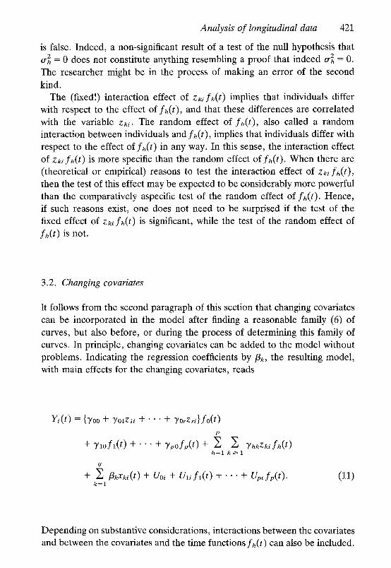
As constant covariates, I have looked at gender, education, and age. It turned out that age did not have a significant effect. Gender had a main effect, but no effects on the individual trend parameters. Looking at formulae (9) and (10) shows that the latter effects are represented by the gender x year and the gender x year 2 interactions. Model 4, of which the estimates are presented in Table 4, is the model in which gender is included. The main effect of gender is highly significant (X 2 = 24.9, d.f. = 1).

Education is expressed as a z-score, with mean 0 and variance 1. Education has an effect more on the trend, especially the quadratic trend, than on the mean of the individual curve. Model 5 includes effects of education on ~'oi, ~rli, and ~'2i. The parameter estimates for this model are also given in Table 4. The joint effect of these three additional parameters is significant (X 2- = 8.5, d.f. = 3, p < 0.05). To interpret the estimated parameters for the

420 T. Snijders

Table 4. Neuroticism: effects of gender and education

Model 4 Model 5

Parameter Variable Estimate S.E. Estimate S.E.

Fixed part Intercept 3'00 8.46 0.32 8.42 0.32 Year dummy 1975 3'30 0.15 0.11 0.15 0.10 Year dummy 1976 3'4o -0.22 0.11 -0.22 0.11 Year dummy 1984 3'2o -0.20 0.13 -0.19 0.13 Year dummy 1986 3"60 0.01 0.14 0.01 0.14 Gender 3'ol 1.01 0.20 1.04 0.20 Education 3'02 -0.04 0.11 Education x year Y12 -0.12 0.08 Education • year z 3'22 0.34 0.15

Random part Variances at level 2 Intercept 0-o0 2.48 0.28 2.48 0.28 Year 0-11 0.89 0.14 0.88 0.14 Year 2 022 2.14 0.53 2.03 0.52 Covariances at level 2 Intercept - year 0"01 -0.08 0.14 -0.09 0.14 Intercept - year 2 0"02 -0.84 0.30 -0.83 0.29 Year - year 2 O"12 0.19 0.18 0.23 0.18 Residual variance 0-~ 0.996 0.066 0.995 0.066

Deviance 4271.9 4263.4

ma in and in te rac t ion effects of educat ion , one could draw a graph of the

expected neuro t ic i sm score as a funct ion of year , for a high, an average, and

a low value of educat ion . G iven the presence of the in te rac t ion terms, the

ma in effect of educa t ion can best be defined not as the statistical pa rame te r

yoz, but as the effect of educa t ion for the average of the 5 observa t ion years,

This can be deno ted by

q

main effect educa t ion = y02 + y12t + y22t 2.

The values of t imply that t = 0.02 and ~ = 0.35, so the ma in effect of

educa t ion is - 0 . 0 4 + ( - 0 . 1 2 • 0.02) + (0.34 x 0.35) = 1.15. This is consider-

able, given that educa t ion is a z-score and the raw s tandard devia t ion of

neuro t ic i sm is abou t 2.

Interactions need not correspond to random effects The ' logic' of this section may suggest that an in te rac t ion te rm zki f~( t ) should be inc luded in the mode l only when the r a n d o m effect of fh(t) is

significant, i .e. , when there is evidence that o-~ is positive. This suggest ion

Analysis of longitudinal data 421

is false. Indeed, a non-significant result of a test of the null hypothesis that o "2 = 0 does not constitute anything resembling a proof that indeed cr~ = 0. The researcher might be in the process of making an error of the second

kind. The (fixed!) interaction effect of zkifh(t) implies that individuals differ

with respect to the effect of fh(t), and that these differences are correlated with the variable z~i. The random effect of fh(t), also called a random interaction between individuals and fh(t), implies that individuals differ with respect to the effect of fh(t) in any way. In this sense, the interaction effect of zki fh(t) is more specific than the random effect of fh(t). When there are (theoretical or empirical) reasons to test the interaction effect of zki fh(t), then the test of this effect may be expected to be considerably more powerful than the comparatively aspecific test of the random effect of fh(t). Hence, if such reasons exist, one does not need to be surprised if the test of the fixed effect of zki fh(t) is significant, while the test of the random effect of fh(t) is not.

3.2. Changing covariates

It follows from the second paragraph of this section that changing covariates can be incorporated in the model after finding a reasonable family (6) of curves, but also before, or during the process of determining this family of curves. In principle, changing covariates can be added to the model without problems. Indicating the regression coefficients by/3k, the resulting model, with main effects for the changing covariates, reads

Yi(t) = {700 + Y01zli + " " + yo, z~i}fo(t) P

+ y~offft) + ' ' " + Ypofp(t) + ~ ~ YhkZkifh(t) h = l k ~ l

q

+ ~ ~kXki(t) + Uoi + Ulifl(t) + ' ' " + Upifp(t). (11) k = l

Depending on substantive considerations, interactions between the covariates and between the covariates and the time functions fh(t) can also be included.

422 T. Snijders

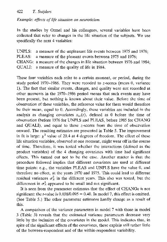
Example: effects of life situation on neuroticism

In the studies by Ormel and his colleagues, several variables have been collected that refer to changes in the life situation of the subjects. We use specifically the next 4 variables:

UNPLS: a measure of the unpleasant life events between 1975 and 1976; PLEAS: a measure of the pleasant events between 1975 and 1976; CHANG: a measure of the changes in life situation between 1976 and 1984; QUALI: a measure of the quality of life in 1984.

These four variables each refer to a certain moment, or period, during the study period 1970-1986. They were recoded to z-scores (mean 0, variance 1). The fact that similar events, changes, and quality were not recorded at other moments in the 1970-1986 period means that such events may have been present, but nothing is known about their value. Before the time of observation of these variables, the reference value for them would therefore be their mean, equal to 0. Accordingly, these variables are included in the analysis as changing covariates xki(t), defined as 0 before the time of observation (before 1976 for UNPLS and PLEAS, before 1985 for CHANG and QUALI), and equal to these z-scores from the time of observation onward. The resulting estimates are presented in Table 5. The improvement in fit is large: X 2 value of 20.4 at 4 degrees of freedom. The effect of these life situation variables, observed at one moment, might wear off in the course of time. Therefore, it was tested whether the interactions (defined as the product variables) of the 4 changing covariates with time had significant effects. This turned out not to be the case. Another matter is that the procedure followed implies that different covariates are used at different time points: e.g., the variables PLEAS and UNPLS have the value 0, and therefore no effect, at the years 1970 and 1975. This could lead to different residual variances or 2 E in the different years. This also was tested, but the differences in ~r 2 appeared to be small and not significant.

It is seen from the parameter estimates that the effect of CHANGe is not significant: the t-value is 0.038/0.095 = 0.40. In model 7, this effect is omitted. (See Table 5.) The other parameter estimates hardly change as a result of this.

A comparison of the variance parameters in model 7 with those in model 3 (Table 3) reveals that the estimated variance parameters decrease very little by the inclusion of the covariates in the model. This indicates that, in spite of the significant effects of the covariates, these explain still rather little of the between-respondent and of the within-respondent variability.

Analysb of longitudinal data Table 5. Neuroticism: effects of life situation

423

Model 6 Model 7

Parameter Variable Estimate S.E. Estimate S.E.

Fixed part Intercept 700 8.48 0.32 8.48 0.32 Year dummy 1975 730 0.15 0.11 0.15 0.11 Year dummy 1976 ]/40 -0.21 0.11 -0.21 0.11 Year dummy 1984 3'50 -0.18 0.12 -0.19 0.12 Year dummy 1986 3'60 0.02 0,13 0.02 0.13 Gender 7ol 1.00 0.20 1.00 0.20 Education Yo2 -0.02 0.I1 -0.02 0.11 Education x year 712 -0,075 0.079 -0.072 0.079 Education x year 2 3'22 0.36 0.15 0.36 0.15 UNPLeaSurable events /31 0.154 0.070 0.154 0.070 PLEASurable events /32 -0.123 0.067 -0.121 0.067 CHANGe in situation /33 0.038 0.095 QUALIty of life /34 -0.315 0.094 -0.329 0.088

Random part Variances at level 2 Intercept oo0 2.44 0.28 2.44 0.28 Year oll 0.81 0.14 0.81 0.14 Year 2 o'22 2.11 0.52 2.11 0.52 Covariances at level 2 Intercept - year ~r m -0.17 0.13 -0.17 0.14 Intercept - year 2 o'o2 -0.90 0.30 -0.90 0.30

Year - year 2 o'12 0.21 0.18 0.21 0.18 Residual variance o~E 0.990 0.065 0.990 0.065

Deviance 4243.0 4243.1

4. Discussion

The Hierarchical Linear Model can be used for analyzing longitudinal data in the format (1), (2). Although still unfamiliar to many researchers in the social sciences, it offers a flexible way of analysis and yields parameters that are quite well interpretable.

For the analysis of neuroticism, we have seen that there are variations over time in neuroticism that can not be explained away as measurement errors, and that these variations are related to the difficult and the pleasant events in a person's life. Also, over the period 1970-1986 in The Netherlands, there is a relationship with education. The quadratic trend is not a pattern that could be meaningfully extrapolated to longer time periods; a conclusion may be that there are ups and downs in neuroticism that can be observed in a person's lifetime over periods of the order of magnitude of 10 years. An

424 T. Snijders

analysis using periodic functions (more specifically, trigonometric functions), or a kind of autocorrelation approach, seem meaningful alternatives to the present approach based on quadratic functions. An analysis with trigono- metric functions was carried out by the author; details are not reported, because this analysis yielded results that were clearly inferior, in terms of model fit, to the analysis reported in this paper. Models incorporating auto- correlation are more complicated, and are treated by Diggle (1988), Jones (1993), and Goldstein et al. (1994).

In this example, the population as a whole is more or less stationary. In other studies, more related to developmental processes, the mean population curve will be more interesting, and the development aspects may pose their own complications for statistical modeling. For example, in studies where the dependent variable grows strongly in the course of the period of study (such as in studies of child length), there may be heteroscedasticity associated with the increase in mean levels. When the researcher uses ML3, heterosced- asticity can be modeled in a quite straightforward fashion.

There is not a single route for the process of specifying an HLM-type model for longitudinal (or other) data. In the example of this paper, a quite empiricist approach was followed. If possible, it is preferable to start with a sensible theory of the studied process and to derive ideas about the model from this theory, prior to the data analysis. The presented approach starts by discovering the random structure of the differences in the individual curves. But the researcher may have a theory pointing toward certain variables and interactions etc., that he or she wishes to make part of the model right from the start. In many instances, this is a better procedure than the empiricist procedure presented above. Another deviation from the examples presented here, which can be useful in other applications, is to use spline functions rather than polynomials to describe the dependency on time. An introduction to the use of spline functions in regression is given in Section 9.5 of Seber and Wild (1989).

Given the availability of parallel measurements for the outcome variable (which is the case for the present data set), an additional level could be added as the lowest one, in order to know how much of the residual variance is measurement variance, and how much is true, unexplained variance. The question of how to define a concept of 'proportion of variance explained' in this type of model (treated in Snijders and Bosker (1994) for multilevel designs with individuals nested in groups) was not treated in this paper. One of the reasons is that, however defined, the proportion of variance explained in the data set used here as an example is not extremely high; this can be seen from the moderate reduction in the variance parameters when going from model 3 to model 7. Any definition of 'proportion of variance explained'

Analysis of longitudinal data 425

has to be based, in some way, on the proportional reduction in these para-

meters. Not only parallel measurements, but also more general multivariate depen-

dent variables can be incorporated in an analysis using the HLM by adding an additional, lowest, level.

The analyses presented above were done using ML3. The other two pro- grams, VARCL and HLM, could also have been used; no options were used that are specific to ML3 and unavailable in the other programs. Readers who ale interested in the use of ML3 for this type of analysis can obtain from the author an annotated log-file of the analyses presented.

The numerical efficiency of procedures for estimating hierarchical linear rnodels can be affected considerably by the choice of the time functions fh(t) that have random effects. Orthogonal, or approximately orthogonal, functions usually have good numerical properties in this respect. However, approximate orthogonality is not necessary. In the example of this paper, powers t p of a time variable were used in such a way, that t assumed values in a range that is approximately symmetric around 0. This also led to very quick convergence of the iterative algorithm used for estimation.

Added in proof. The ML3 program has now been succeeded by MLn.

Acknowledgments

I am grateful to Hans Ormel for the permission to use his data on neuroticism for examples in this paper. I also extend my thanks to colleagues, too many to be mentioned, who gave comments on earlier drafts.

References

Alasker, F.D. (1992). Modeling quantitative developmental change, in J.B. Asendorpf & J. Valsiner (eds.), Stability and Change in Development. Newbury Park: Sage, pp. 88-109.

Bryk, A.S., Raudenbush, S.W., & Congdon, R.T. (1994). HLM 2.13: Hierarchical Linear Modeling with the HLM/2L and HLM/3L Programs. Chicago: Scientific Software Interna- tional.

Bryk, A.S. & Raudenbush, S.W. (1992). Hierarchical Linear Models, Applications and Data Analysis Methods. London: Sage.

Dale, A. & Davies, R.B. (1994). Analyzing Social and Political Change. London: Sage. Diggle, P.J. (1988). An approach to the analysis of repeated measurements, Biometrics 44: 959-

971. Diggle, P.J., Liang, K.-Y., & Zeger, S.L. (1994). Analysis of Longitudinal Data. Oxford:

Clarendon Press.

426 T. Snijders

Goldstein, H. (1987). Multilevel Models in Educational and Social Research. London: Charles Griffin & Co.

Goldstein, H. (1989). Flexible models for the analysis of growth data with an application to height prediction, Revue d'Epiddmiologie et Santd Publique 37: 477-484.

Goldstein, H., Healy, M.J.R., & Rasbash, J. (3_994). Multilevel time series models with appli- cations to repeated measures data, Statistics in Medicine 13: 1643-1655.

Hoeksma, J.B. & Koomen, M.Y. (1992). Multilevel models in developmental psychological research: rationales and applications. Early Development and Parenting 1: 157-167.

Hsiao, C. (1986). Analysis of Panel Data. Cambridge: Cambridge University Press. Jones, R.H. (1993). Longitudinal Data with Serial Correlation: A State Space Approach. London:

Chapman and Hall. Kmenta, J. (1986). Elements of Econometrics, 2nd ed. New York: MacMillan. Laird, N.M. & Ware, J.H. (1982). Random-effects models for longitudinal data', Biometrics

38: 963-974. Lindsey, J.K. (1993). Models for Repeated Measurements. Oxford: Clarendon Press. Longford, N.T. (1993). VARCL: Software for Variance Component Analysis of Data with Nested

Random Effects (maximum likelihood). Manual. Groningen: ProGAMMA. Maas, C. & Snijders, T.A.B. (1995). Analysis of repeated measures with missing data using the

Hierarchical Linear Model, forthcoming. Marsh, H.W., & Grayson, D. (1994). Longitudinal confirmatory factor analysis: common,

time-specific, item-specific, and residual-error components of variance, Structural Equation Modeling 1: 116-145.

Ormel, J. & Schaufeli, W.B. (1991). Stability and change in psychological distress and their relationship with self-esteem and locus of control: a dynamic equilibrium model, Journal of Personality and Social Psychology 60: 288-299.

Ormel, J. & Wohlfarth, T. (1991). How neuroticism, long-term difficulties, and life situation change influence psychological distress: a longitudinal model, Journal of Personality and Social Psychology 60 744-755.

Plewis, I. (1994). Longitudinal multilevel models, in A. Davis and R.B. Davies (eds.), Analyzing Social and Political Change. London: Sage.

Prosser, R., Rasbash, J., & Goldstein, H. (1991). ML3: Software for Three-level Analysis. London: Institute of Education, University of London.

Raudenbush, S.W. & Chart, W.-S. (1994). Application of a hierarchical linear model to the study of adolescent deviance in an overlapping cohort design, Journal of Consulting and Clinical Psychology 61: 941-951.

Rogosa, D., Brandt, D., & Zimowski, M. (1982). A growth curve approach to the measurement of change, Psychological Bulletin 92: 726-748.

Rogosa, D.R. & Willett, J.B., (1985). Understanding correlates of change by modeling indivi- dual differences in growth, Psychometrika 5o: 203-228.

Rutter, C.M., & Elashoff, R.M. (1994). Analysis of longitudinal data: Random coefficient regression modelling, Statistics in Medicine 13: 1211-1231.

Seber, G.A.F., & Wild, C.J. (1989). Nonlinear Regression. New York: Wiley and Sons. Snijders, T.A.B. & Bosker, R.J. (1994). Modeled variance in two level models, Sociological

Methods and Research 22: 342-363. Sternio, J.L.F., Weisberg, H.I., & Bryk, A.S. (1983). Empirical Bayes estimation of individual

growth curves parameters and their relationship to covariates, Biometrics 39: 71-86. Swamy, P.A.V.B. (1974). Linear models with random coefficients, in P. Zarembka (ed.),

Frontiers in Econometrics. New York: Academic Press. Willett, J.B. & Sayer A.G. (1994). Using covariance structure analysis to detect correlates and

predictors of individual change over time, Psychological Bulletin 116: 363-381.