Embed Size (px)
Citation preview
ANALYSIS OF LEAN PREMIXED TURBULENT COMBUSTION USING
COHERENT ANTI-STOKES RAMAN SPECTROSCOPY
TEMPERATURE MEASUREMENTS
by
Daniel V. Flores
A dissertation submitted to the faculty of
Brigham Young University
In partial fulfillment of the requirements for the degree of
Doctor of Philosophy
Department of Chemical Engineering
Brigham Young University
April 2003

BRIGHAM YOUNG UNIVERSITY
GRADUATE COMMITTEE APPROVAL
Of a dissertation submitted by
Daniel V. Flores
This dissertation has been read by each member of the following graduate committee and by a majority vote has been found satisfactory. _____________________________ ____________________________________ Date Thomas H. Fletcher, Chair _____________________________ ____________________________________ Date Paul O. Hedman _____________________________ ____________________________________ Date Merrill W. Beckstead _____________________________ ____________________________________ Date William G. Pitt _____________________________ ____________________________________ Date Kenneth A. Solen
BRIGHAM YOUNG UNIVERSITY
As chair of the candidate’s graduate committee, I have read the dissertation of Daniel V. Flores in its final form and have found that (1) its format, citations, and bibliographical style are consistent and acceptable and fulfill university requirements; (2) its illustrative materials including figures, tables, and charts are in place; and (3) the final manuscript is satisfactory to the graduate committee and is ready for submission to the university library. _____________________________ ____________________________________ Date Thomas H. Fletcher Chair, Graduate Committee Accepted for the Department
____________________________________ William G. Pitt Graduate Coordinator Accepted for the College
____________________________________ Douglas M. Chabries Dean, College of Engineering and Technology

ABSTRACT
ANALYSIS OF LEAN PREMIXED TURBULENT COMBUSTION USING
COHERENT ANTI-STOKES RAMAN SPECTROSCOPY
TEMPERATURE MEASUREMENTS
Daniel V. Flores
Department of Chemical Engineering
Doctor of Philosophy
An existing CARS instrument was modified to use a new dual dye laser that produces
simultaneously CARS spectra of N2, CO, CO2 and O2. These CARS spectra yield
simultaneous values for the gas temperature from N2 and concentrations of CO, CO2 and
O2. The dual-dye laser was generated using a mixture of pyromethene 650 and 597 dyes
(both commercially available) dissolved in ethanol. Calibration studies in a tube furnace
showed that the modified CARS instrument using the dual dye laser has good accuracy
and acceptable precision for gas temperature measurements. However, the modified
instrument had limited capabilities in measuring the concentrations of O2 and CO2 in the
concentration ranges of interest, possibly due to the approximations involved in the
CARS reduction algorithm used in this work.
The modified CARS instrument was successfully applied to obtain detailed
measurements of instantaneous gas temperature for four lean premixed combustion
conditions, with varying inlet stoichiometry and swirl level, in a Laboratory Scale Gas
Turbine Combustor (LSGTC). The temperature data were used to produce iso-contour
plots of averaged and normalized standard deviations. Probability Density Function
(PDF) plots were also produced at several measurement locations.
Additional insights regarding the flame behavior were obtained by examining the
spatial variation in the shape of the PDFs for all the combustion conditions. Several
zones were identified in all four cases where the nature of the PDFs seems to be
determined by different factors. At lower heights, near the bottom of the combustor, the
swirl level seems to be the predominant factor determining the nature of the turbulent
fluctuations, whereas near the wall and around z = 50 mm, the equivalence ratio appears
to predominate. For the rest of the flame, the combined effect of the equivalence ratio
and swirl level seems to determine the nature of the temperature fluctuations.
A preliminary analysis of combined LDA, PLIF and CARS data was presented for the
most stable combustion case. The combined analysis made it possible to identify a
potential zone of ignition, started by the mixing with the hot gases from both the central
and the side recirculation zones.
Analysis of the gas temperature data has revealed new insights into the complex
nature of the mixing and reaction processes that take place in lean premixed swirling
flames. Comparison with LDA velocities and PLIF OH images suggests that the side
recirculation zone may play an important role in the stabilization of the flame, along with
the central recirculation zone. In addition, a flow reversal observed in the velocity
components suggests the existence of eddies throughout the flame.

For my dad Para mi papá
José Flores A. 1940 - 2002

ACKNOWLEDGEMENTS
I feel deeply indebted to many people, first, to my beloved wife, Susan, and our
children who put up with many a “well, I need to go work on my dissertation” from me.
Equally as important I am indebted to my dad, whose vision, courage, and
encouragement made this possible: gracias papá. Then there is a long list of other good
people: Dr. Fletcher and Dr. Hedman for their PATIENCE and guidance; Ken Foster in
the machine shop for making himself and his shop available for me to fix broken parts
and make others as I needed them; and Stewart Graham and Wayne Timothy, two
undergraduate students, for their valuable assistance. Finally, I also thank the
Department of Chemical Engineering, the College of Engineering and Technology, and
Brigham Young University for providing excellent professors, research assistantships,
and scholarships.
viii
TABLE OF CONTENTS
1. INTRODUCTION ......................................................................................................1 1.1 Background ..........................................................................................................1 1.2 Objectives ............................................................................................................2 1.3 Approach..............................................................................................................2
2. LITERATURE REVIEW ...........................................................................................5
2.1 Combustion Issues in Gas Turbines ....................................................................5 2.2 Laser Diagnostics Techniques .............................................................................7 2.3 Development and Applications of the CARS Technique ..................................12 2.4 CARS Measurements in Gas Turbine Combustors ...........................................13 2.5 Previous Experimental Studies on Premixed Natural Gas/Air Combustion .....15 2.6 Previous Premixed Combustion Studies Related to This Work ........................21
3. THE BYU DUAL DYE SINGLE STOKES CARS INSTRUMENT......................23
3.1 CARS Instrument Description...........................................................................23 3.2 The Dual Dye Single Stokes Laser ....................................................................31
3.2.1 Development ..............................................................................................31 3.2.2 Advantages and Limitations ......................................................................35
4. CARS SPECTRA INTERPRETATION ..................................................................39
4.1 Spectra Preprocessing ........................................................................................39 4.1.1 Obtaining the CARS Spectrum from Recorded Spectra............................39
4.1.1.1 IPDA Image Persistence ........................................................................41 4.1.1.2 IPDA Detector Non-Linearity ...............................................................43
4.1.2 Obtaining the CARS Susceptibility From the CARS Spectrum................45 4.2 Accounting for Other Instrumental Dependencies ............................................47
4.2.1 Spectrometer Dependencies.......................................................................48 4.2.1.1 Spectral Dispersion................................................................................48 4.2.1.2 Instrument Function...............................................................................51
4.2.2 Pump Laser Dependency...........................................................................56 4.3 Fitting Methodology ..........................................................................................57
4.3.1 Computation of Concentrations and Temperature.....................................59 4.4 Software Developed in This Work ....................................................................61
5. ACCURACY AND PRECISION OF THE BYU SINGLE-STOKES DUAL
DYE CARS INSTRUMENT....................................................................................65 5.1 Temperature .......................................................................................................65 5.2 O2 Concentrations ..............................................................................................73
ix
5.3 CO2 Concentrations ...........................................................................................77 6. EXPERIMENTAL PROGRAM...............................................................................81
6.1 Combustion Conditions .....................................................................................86 6.2 CARS Data Acquisition.....................................................................................88
7. RESULTS AND DISCUSSION...............................................................................91
7.1 CARS Temperature Contours ............................................................................91 7.1.1 Average Gas Temperature .........................................................................92
7.1.1.1 Flame Stability Observations ...............................................................100 7.1.2 Turbulent Fluctuations in the Gas Temperature: Standard Deviations ...102 7.1.3 Gas Temperature Turbulent Fluctuations: Probability Density
Functions ..................................................................................................109 7.2 Comparison of CARS, PLIF and LDA data ....................................................119 7.3 Suggestions for Future Research.....................................................................130
8. CONCLUSIONS AND RECOMMEDATIONS....................................................133
8.1 Conclusions ......................................................................................................133 8.2 Recommendations ............................................................................................137
9. REFERENCES .......................................................................................................139 10. APPENDIXES ........................................................................................................145
x
LIST OF FIGURES
Figure 2.1. Simplified schematic of a gas turbine system. .................................................6
Figure 2.2. Rayleigh and Raman Scattering processes. ......................................................9
Figure 2.3. BOXCARS configuration to produce a CARS signal....................................11
Figure 2.4. Variation of adiabatic temperature with φ......................................................21
Figure 2.5. Recirculation patterns in the LSGTC. ............................................................22
Figure 3.1. Schematic of the BYU dual dye single Stokes CARS instrument. .................24
Figure 3.2. Spectral profile of the dual dye single Stokes laser. .......................................32
Figure 4.1. A raw multi-species CARS measurement and its corresponding background-subtracted spectrum. ...................................................................40
Figure 4.2. A sample dye profile from the BYU single Stokes dual dye CARS instrument. ......................................................................................................47
Figure 4.3. A comparison of theoretical and experimental CARS spectra.......................49
Figure 4.4. Xenon spectrum obtained by the spectrometer used in this research. .............50
Figure 4.5. Broadening of a monochromatic line by a spectrometer having a symmetric Gaussian instrument function. ......................................................52
Figure 4.6. The asymmetric N2 instrument function calculated for the spectrometer used in this research. .......................................................................................54
Figure 4.7. Algorithm to calculate temperatures and mole fractions from measured CARS spectra .................................................................................................64
Figure 5.1. CARS-Measured Temperatures vs. Thermocouple values in a calibration tube furnace. ...................................................................................................68
Figure 5.2. PDFs of gas temperature (K) measured in air using the BYU single Stokes instrument. ......................................................................................................70
Figure 5.3. Examples of two different CO2 FMCARS fits on the same experimental CO2 spectrum..................................................................................................79
Figure 6.1. Schematic of the LSGTC at BYU. .................................................................82
Figure 6.2. Schematics of a) premixer and b) swirl blocks on the LSGTC......................84
Figure 6.3. Spatial grids for data acquisition on the LSGTC combustor. ........................89
Figure 7.1. Contour maps of mean gas temperatures for the MS65 case. ........................93
xi
Figure 7.2. Contour maps of mean gas temperatures for the MS80 case. ........................94
Figure 7.3. Contour maps of mean gas temperatures for the HS65 case. .........................95
Figure 7.4. Contour maps of mean gas temperatures for the HS80 case. .........................96
Figure 7.5. Axial temperature profiles at selected radial positions for the HS80 case .....98
Figure 7.6. Radial temperature profiles at selected heights for the HS80 case. ...............99
Figure 7.7. Contour maps of normalized standard deviation gas temperature for the MS65 case. ...................................................................................................103
Figure 7.8. Contour maps of normalized standard deviation gas temperature for the MS80 case. ...................................................................................................104
Figure 7.9. Contour maps of normalized standard deviation gas temperature for the HS65 case. ....................................................................................................105
Figure 7.10. Contour maps of normalized standard deviation gas temperature for the HS80 case...................................................................................................106
Figure 7.11. Characteristic heights of complete combustion and cessation of fluctuation, plotted as a function of φ. .......................................................107
Figure 7.12. Types of PDF distributions in the combustion experiments. .....................110
Figure 7.13. Gas temperature PDFs as a function of radial position for z = 10 mm. .....111
Figure 7.14. Gas temperature PDFs as a function of radial position for z = 50 mm. .....112
Figure 7.15. Gas temperature PDFs as a function of radial position for z = 70 mm. .....113
Figure 7.16. Gas temperature PDFs as a function of radial position for z = 90 mm. .....114
Figure 7.17. Location of the bimodal distribution PDFs for all combustion cases ........118
Figure 7.18. Averaged axial/radial velocity vector plot superimposed on the averaged CARS gas temperature map (left) and the average PLIF OH intensity image (right) for the HS80 case. .................................................121
Figure 7.19. Samples of instantaneous OH PLIF images for the HS80 case. ................123
Figure 7.20. Example temperature PDFs for the HS80 case. .........................................125
Figure 7.21. Example PDFs from OH-PLIF images for the HS80 case. ........................126
Figure 7.22. Sample PDFs of the axial velocity components for the HS80 case. ..........127
xii
LIST OF TABLES
Table 2.1. Summary of experimental studies on turbulent combustion of premixed natural gas and air reported in the literature. ...................................................16
Table 3.1. Purpose of CARS instrument components. .....................................................25
Table 3.2. Changes in pyromethene dye concentrations in ethanol during the development of the dual dye single Stokes laser. ............................................35
Table 4.1. Voigt and Lorentzian widths for the asymmetric instrument functions of N2, O2 and CO2 in the spectrograph used in this work ....................................55
Table 5.1. Comparison CARS temperature measurements and thermocouple readings in a calibration tube furnace. ...........................................................................68
Table 5.2. Empirically corrected CARS temperature measurements vs. thermocouple readings in a calibration tube furnace. .............................................................71
Table 5.3. CARS O2 concentration measurements in a calibration tube furnace. ............74
Table 6.1. Chemical composition of the natural gas available for the LSGTC experiments......................................................................................................85
Table 6.2. Operating conditions investigated using the LSGTC. .....................................87
Table 7.1. Characteristic flame heights and range of normalized standard deviations for each combustion case. ..............................................................................107
Table 7.2. Relative occurrence (%) of PDF shapes for each combustion case. .............115
Table 7.3. Example LDA velocity data statistics at various locations for the HS80 case.................................................................................................................128
xiii
NOMENCLATURE
Acronyms
CARS Coherent Anti-Stokes Raman Spectroscopy
CRZ Central Recirculation Zone
FWHM “Full Width at Half Maximum”, i.e., the total width of the line shape at half the value of the maximum intensity
IPDA Intensified Photo-Diode Array
LDA Laser Doppler Anemometry
LSGTC Laboratory-Scale Gas Turbine Combustor
PDF Probability Density Function
PLIF Planar Laser Induced Fluorescence
SRZ Side Recirculation Zone
Symbols and Variables
D diameter of a beam prior to focusing on the diagnostic volume
d LSGTC swirl block nozzle diameter
dh LSGTC swirl block vane hub diameter
sd CARS sampling volume diameter
lf focal length of the focusing lens
f , g convolution functions of the resonant components of theoryCARS ,χ
HS65 Combustion case of High Swirl φ = 0.65
HS80 Combustion case of High Swirl φ = 0.80
I background-free intensity values of a single-shot CARS sample corrected for image persistence from the previous sample
bgI averaged sample of background noise across the wavelength range of the IPDA

xiv
bgFreeI background-free spectral curve
PrevbgFreeI , background-free intensity values of the previous single-shot CARS sample
CARSI estimated actual CARS spectrum
dyeI intensity of the dye laser as a function of wavelength, theoretical
dyeProfileI intensity of the dye laser as a function of wavelength, measured
pumpI intensity of the pump laser
rawI spectra recorded by the BYU single-Stokes CARS instrument
ωI light intensity at the frequency ω at either side of 0ω
0ωI light intensity at the actual frequency 0ω
ImaPer residual intensity in a CARS sample due to image persistence from the previous sample
L CARS sampling volume length
NonLin the non-linearity of the IPDA used in this work
MS65 Combustion case of Medium Swirl φ = 0.65
MS80 Combustion case of Medium Swirl φ = 0.80
iP ith pixel in the IPDA
SN Swirl Number, the ratio of the tangential momentum to the axial momentum
ix mole fractions of the ith species (e.g., N2, O2 or CO2) in the CARS sample mixture
r radial distance measured from the centerline of the LSGTC
z vertical height measured from the bottom of the LSGTC chamber
CARSχ experimental CARS susceptibility obtained from CARSI
theoryCARS ,χ theoretical CARS susceptibility, fitted to its experimental counterpart
CARSχ
NRχ total nonresonant susceptibility component of theoryCARS ,χ
lω∆ Lorentzian FWHM for the approximated Voigt function, in cm-1.
Rω∆ Raman Shift of a molecular transition
iR,ω∆ Raman Shift in cm-1 at the ith pixel
xv
vω∆ Voigt FWHM for the approximated Voigt function, in cm-1.
φ Fuel equivalence ratio
λ light wavelength
iλ wavelength of the light reaching the ith IPDA pixel
θ LSGTC swirl block vane angle measured from the vertical axis
1ω pump beam frequency
2ω dye beam frequency
3ω CARS signal frequency

1
1. INTRODUCTION
1.1 Background
During the past few years, turbine systems operating on natural gas have been
considered as a viable alternative to produce electricity, which is greatly needed by our
society. Turbine systems may operate using a wide variety of fuels; however, the large
amounts of natural gas available and its relatively clean combustion characteristics make
it an attractive fuel as a source of energy (Ecob, et al., 1996; Hay, 1985).
In an effort to improve the technology of gas turbine systems, the U. S. Department of
Energy started the Advanced Turbine Systems (ATS) program. The ATS program has
the objective of developing and commercializing land-based gas turbine systems that are
1) highly efficient, 2) environmentally superior, and 3) cost competitive. Because of the
complexity of the task, several industrial and educational institutions are involved in the
ATS program doing research in different key aspects of the performance of gas turbine
systems. One of those key aspects is the combustion in the gas turbine, which largely
determines both the efficiency and the pollutant emissions of the engine.
An ATS contract (Hedman, et al., 1998) to develop a computer code for modeling
combustion in gas turbine systems was granted to the Advanced Combustion Engineering
Center (ACERC) at Brigham Young University (BYU). The primary focus of the ATS
research at ACERC was the simulation of the turbulent combustion of natural gas
premixed with air in gas turbines. However, the ATS research at ACERC also included a

2
comprehensive experimental program dedicated to the acquisition of reliable
experimental data to help in 1) understanding the combustion process in conditions
relevant to advanced gas turbine systems; and 2) va lidating the computer simulations.
This work is one in a series of laser-diagnostics experiments performed as part of the
ATS research at ACERC. The other two parts of the study consist of (a) gas velocity
measurements (Hedman, et al., 2002b; Murray, 1998), and (b) OH radical imaging
(Hedman, et al., 2002a), both obtained using laser diagnostics techniques.
1.2 Objectives
This work had three main objectives. The first objective was the development of a
novel variation of a laser diagnostics instrument. The second objective was to apply the
new instrumentation to obtain instantaneous gas temperature measurements in a burner
configuration relevant to practical gas turbine combustors. The third objective was to use
the temperature data to examine the effects of swirl and stoichiometry on the premixed
combustion within the fuel- lean range.
It is expected that the data obtained in this work, together with the other two parts of
the ATS study, will lead to a better understanding of the complex interactions between
turbulence, chemical kinetics, heat transfer, and flow dynamics during lean premixed
turbulent combustion. The data will also serve as a benchmark, aiding combustion
modelers in the development and evaluation of comprehensive computer models.
1.3 Approach
The combustion of premixed natural gas with air was investigated at four different
conditions of stoichiometry and inlet swirl. The experiments were performed in the
3
Laboratory Scale Gas Turbine Combustor (LSGTC) located in the optics laboratory at
BYU. The LSGTC simulates many of the combustion characteristics of industrial gas
turbine combustors while providing appropriate optical access for laser diagnostics
techniques.
In this work, measurements were carried out using Coherent Anti-Stokes Raman
Spectroscopy (CARS), a non- intrusive laser based technique. The CARS instrument
developed in this work was based on previous research on a dye laser reported by Haslam
and Hedman (1996) that allows simultaneous CARS measurements of N2, CO, CO2, and
O2 spectra. These CARS spectra yield simultaneous values for the gas temperature and
concentrations of CO, CO2, and O2.
Furthermore, a brief comparison of the CARS temperature data with velocity data
(Hedman, et al., 2002b; Murray, 1998) and OH data (Hedman, et al., 2002a) was
performed. Some interesting insights were gained from this comparison leading to some
suggestions for further research.

4
5
2. LITERATURE REVIEW
2.1 Combustion Issues in Gas Turbines
The basic operation of gas turbine systems (see Figure 2.1) can be described as
follows (Lefebvre, 1983): 1) atmospheric air is compressed to high pressures; 2)
practical gas turbine systems mix the high-pressure air and the fuel prior to combustion;
3) the premixed fuel/air mixture is then injected into the combustion chamber at high
swirling velocities; 4) the hot gases produced in the burner are then carried into the
turbine blades that convert the thermal energy to shaft work, which can be used to
generate electricity.
The combustion chamber is a critical component of a gas turbine system since it
determines the emission levels of pollutants and plays a determinant role on overall
efficiency and turbine durability. Thus, it is important to understand the impact of the
combustion process on burner configurations relevant to gas turbine systems.
The gas turbine combustion chamber must be designed to comply with several
operational criteria. These criteria arise because of requirements relative to structural
stability of the turbine, existing environmental regulations, and overall efficiency of the
gas turbine system.
The main design criteria for burner design may be summarized as follows (Cohen, et
al., 1996; Melvin, 1988): 1) the temperature of the exit stream gases must be sufficiently
low to keep stress on turbine components within specifications; 2) the temperature

6
Compressor Turbine
Fuel
Combustion chamber
Exhaust gas
Power output
Air
Figure 2.1. Simplified schematic of a gas turbine system. distribution of the exit stream gases must be known to avoid local overheating on turbine
blades; 3) stable combustion must be maintained at high air velocities (30-60 m/s) and
over the range of air/fuel ratios that the combustor will experience between full load and
idling conditions; 4) the production of soot must be avoided because of particulate
emissions restrictions (visual plumes) and the potential of damaging engine components
and blocking cool air passages; 5) emission levels of pollutants such as nitrogen oxides
(NOx), carbon monoxide (CO), and unburned hydrocarbons (UHC) must conform to
environmental regulations; and 6) high performance and efficiency of the gas turbine
system must be maintained.
Designing a burner configuration that offers optimum performance is challenging
because conditions favoring one criterion may work against another. For example,
increasing the turbine inlet temperature and operating at high pressures increases the
efficiency but also increases the production of undesirable NOx.
Clearly, a good quantitative understanding of turbulent premixed combustion of
natural gas and air is required in order to design combustors with optimum performance.
7
In achieving such understanding, complete experimental studies under conditions
relevant to gas turbine systems must be performed. The results of such experimental
knowledge can be used to understand fundamental aspects of premixed combustion as
well as to validate comprehensive computer codes that will aid in combustor design.
2.2 Laser Diagnostics Techniques
The experimental analysis of clean gaseous flames, such as premixed natural gas
flames relevant to gas turbines, can be carried out using a variety of methods. Laser
diagnostics techniques are considered the most suitable because they provide a non-
intrusive means of analyzing the gas-phase combustion, both spatially and temporally.
Existing laser diagnostics techniques allow the measurement of gas velocities,
temperatures, and concentrations of chemical species.
Gas velocities can be measured using Laser Doppler Anemometry (LDA), a very well
established technique (e.g. Murray, 1998; Schmidt, 1995; Schmidt and Hedman, 1995;
Warren and Hedman, 1995; Warren, 1994). LDA is based upon the Mie scattering from
particulates crossing a control volume defined at the focusing point of two lasers of the
same wavelength (Rudd, 1969; Yeh and Cummins, 1964), usually in the visible range.
Because the laser source is generally continuous, the rate of data acquisition depends on
the rate that particles cross the control volume. Two components of the velocity field can
be obtained simultaneously by focusing two pairs of lasers at the same point, each pair
having a different color.
Using the aforementioned two-color technique, Murray (1998) obtained two sets of
time-resolved gas velocity measurements on the LSGTC for the same combustion
conditions to be investigated in this work. One set of velocity measurements consisted of

8
simultaneous measurements of axial and radial velocity components whereas the other set
was for the axial and tangential velocity components. It must be noted that there are no
inherent particles in a premixed natural gas and air system, and, therefore, the flame must
be seeded with inert particles that are small enough to follow the flow. A description of
the particle type and loading used in the LDA measurements on the LSGTC is given by
Murray (1998). This particle seeding may be considered an intrusion to the flow, but its
effects on the flow and the combustion are considered minimal because the particles are
inert hollow Al2O3 spheres with an average diameter of 6 µm.
The most prominent laser spectroscopic techniques for measuring gas temperature
and species concentrations (Eckbreth, 1996) are: Rayleigh scattering, Raman scattering,
Planar Laser Induced Fluorescence (PLIF), and Coherent Anti-Stokes Raman
Spectroscopy (CARS). The first three techniques have the following common features:
1) only one laser is required to generate the signal and 2) they are incoherent in that the
signal is scattered in all 4p steradians from each point along the path of the laser, which
limits the signal collection to only a fraction of the total. In contrast, CARS requires the
use of three lasers to generate a coherent (i.e., laser- like) signal that can be collected in its
entirety. CARS is a very well established technique in the study of combustion
(Eckbreth, 1996; Tolles, et al., 1977) and is the technique used in this work. Brief
descriptions of the other techniques follow. More information on these techniques, and
others not mentioned here, may be found elsewhere (Eckbreth, 1996).
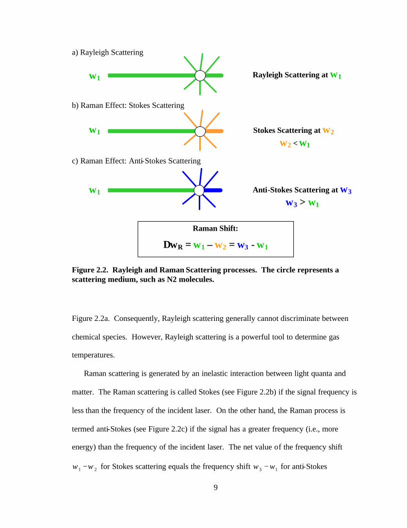
Rayleigh scattering results when light quanta interact with molecules in an elastic
process, i.e., there is no net energy exchange between the light and the molecules. Thus,
the Rayleigh signal has the same frequency as that of the incident light, as shown in
9
a) Rayleigh Scattering
b) Raman Effect: Stokes Scattering
c) Raman Effect: Anti-Stokes Scattering
Figure 2.2. Rayleigh and Raman Scattering processes. The circle represents a scattering medium, such as N2 molecules. Figure 2.2a. Consequently, Rayleigh scattering generally cannot discriminate between
chemical species. However, Rayleigh scattering is a powerful tool to determine gas
temperatures.
Raman scattering is generated by an inelastic interaction between light quanta and
matter. The Raman scattering is called Stokes (see Figure 2.2b) if the signal frequency is
less than the frequency of the incident laser. On the other hand, the Raman process is
termed anti-Stokes (see Figure 2.2c) if the signal has a greater frequency (i.e., more
energy) than the frequency of the incident laser. The net value of the frequency shift
21 ωω − for Stokes scattering equals the frequency shift 13 ωω − for anti-Stokes
Rayleigh Scattering at ω1
Stokes Scattering at ω2
ω2 < ω1
Anti-Stokes Scattering at ω3
ω3 > ω1
Raman Shift:
∆ωR = ω1 – ω2 = ω3 - ω1
ω1
ω1
ω1
10
scattering. This “Raman shift”, Rω∆ , is a distinctive molecular property and allows the
use of Raman scattering to measure temperatures and, in principle, concentrations of any
Raman-active species with the use of only one laser. However, Raman scattering is
limited in practice by the sensitivity of current detectors because of their low signal- to-
noise ratios, which is compounded with the signal being scattered in all directions.
Planar Laser Induced Fluorescence (PLIF) is achieved by exciting the species of
interest to a higher electronic state by means of a laser sheet. The excited species then
undergoes the process of fluorescence by spontaneously emitting light as it returns to the
ground state. Thus, a 2-dimensional image of the species being probed can be collected.
PLIF has found great application in the diagnostics of radicals and species whose
concentrations are below the 1000 ppm level, where other techniques fail. However, a
quantitative interpretation of PLIF images still remains a challenge due to various factors
that are beyond the scope of this review (Eckbreth, 1996).
Coherent Anti-Stokes Raman Spectroscopy (CARS) is based on the generation of a
Raman induced signal at the anti-stokes frequency of the species being probed. In a
sample of molecules of the same species, there are several combinations of rotational and
vibrational states, each state having its own CARS signal. This set of CARS signals
forms the CARS spectrum, which is specific for a given species and varies with
temperature. The CARS signal is generated by aligning three laser beams of appropriate
frequencies in any geometrical arrangement that complies with the “phase matching”
condition (Eckbreth, 1996).
Figure 2.3 shows the geometrical arrangement commonly known as BOXCARS that
is used at the BYU optics laboratory. This arrangement focuses the three beams onto a

11
Figure 2.3. BOXCARS configuration to produce a CARS signal diagnostic volume about 1 mm long and 20 µm in diameter. In general, two of the lasers
will be at the same frequency (ω1); these lasers are commonly called “pump” beams.
The third laser of frequency ω2 is commonly referred to as the “Stokes” laser because
it must be “Stokes-shifted” from frequency ω1 to generate one of the possible CARS
signals of a species. This means that ω2 must equal the frequency the “pump” beams
minus the Raman shift of the species being probed. The CARS signal is then generated
at the frequency ω3, the anti-Stokes Raman transition relative to the pump beams. For
time-resolved diagnostics, as in this research, all of the CARS signals (i.e., the CARS
spectrum) of each of the species of interest must be obtained simultaneously. This
requires the spectral energy distribution of the Stokes beam to cover all the Stokes Raman

12
transitions of one or more species, which requirement can be achieved by the use of
broadband dye lasers.
A more detailed explanation of the theory of CARS is beyond the scope of this
dissertation; however, there are several sources available in the literature (Eckbreth,
1996; Druet and Taran, 1981; Eesley, 1981; Tolles and Harvey, 1981; Tolles, et al., 1977;
Armstrong, et al., 1962). CARS has been shown to be particularly useful in thermometry
and in the detection of major species (i.e., species whose molar percentage is greater than
1%) in a broad range of combustion environments. The CARS signal is several orders of
magnitude greater than the spontaneous Raman signal, with a much better signal-to-noise
ratio as well. A brief review of the development and applications of CARS is given
below.
2.3 Development and Applications of the CARS Technique
The application of the CARS technique to combustion and gas phase diagnostics was
pioneered by Taran and co-workers (e.g., Moya, et al., 1975; Regnier and Taran, 1973) at
the Office National d’Etudes et de Recherches Aerospatiales (ONERA) France. Interest
in the technique grew very quickly in the scientific community with many advances
having been made over the last two decades. Eckbreth (1996) summarizes in detail many
of the major improvements on CARS technology, which include instrument
modifications as well as code development for CARS signal interpretation. At present,
CARS is a well-established technique in the study of combustion. Some industrially-
relevant combustion systems where the CARS technique has been used (Eckbreth, 1996)
include premixed gaseous flames, diffusion flames (gaseous and liquid), internal
combustion engines, sooting flames, coal flames, solid propellant rocket flames,
13
supersonic flows, jet engine exhausts, and model gas turbine combustors. A summary of
a few CARS studies performed on turbine combustors is presented in the next section.
2.4 CARS Measurements in Gas Turbine Combustors
An early application of CARS to a model gas turbine combustor was made by
Switzer, et al. (1982) at the Aero Propulsion Laboratory of the Wright-Patterson Air
Force Base. The combustor was a bluff-body stabilized, non-premixed system with the
fuel injected at the center of a cylindrical duct and the air flowing through an annulus
between the duct and the bluff-body. Three different fuels were investigated (gaseous
propane, JP-4 and JP-8) over a wide range of equivalence ratios, all at atmospheric
pressure. CARS measurements were made at different axial positions throughout the
flame, yielding gas temperatures and concentrations of N2 and O2. Furthermore, the
CARS results and those of other sampling techniques were compared in order to establish
the reliability of the CARS technique. Their work demonstrated the applicability of
CARS to make measurements in practical combustion systems.
Bedue and co-workers (1984) made CARS measurements in a combustor designed to
closely simulate a “real jet engine." The combustor operated on kerosene and could be
pressurized up to 6 bar with outlet temperatures in the 1500-2000 K range. The
combustion chamber was rectangular with three fuel injectors in the back wall.
Secondary combustion air and dilution air for cooling were provided through air ports
that were also used for optical access. Radial profiles of gas temperature were obtained
at various positions in the flame. The uncertainty on the measurements was estimated to
be ±50 K. This work also demonstrated the viability of CARS as a measurement
technique in a hostile combustion environment.
14
Zhu, et al. (1993) reported CARS temperature measurements, averaged and root mean
squared, in a liquid-fuel spray combustor operating at atmospheric pressure. The
combustor consisted of a stainless-steel cylindrical chamber with a spray injector
centered on swirling vanes for air injection at the inlet. In addition, secondary and
dilution streams of air were introduced into the chamber. The fuel used in their
experiment was JP-4. Zhu and co-workers reported that the use of CARS was successful,
in spite of the challenge of droplet-induced breakdown near the injector.
Hedman and co-workers (1995) did very extensive experimental work on a
combustor using a Pratt & Whitney injector from a military jet engine. The combustion
chamber was designed to closely simulate the main flow and reaction characteristics of
real jet engine combustors (Sturgess, et al., 1992). The combustor operated at
atmospheric pressure burning non-premixed propane and air. The measurements
included video imaging of the flame, LDA gas velocities, PLIF images of OH radical,
and CARS temperatures. The gas temperature measurements were made at an air flow
rate of 500 standard liters per minute (slpm) and four different inlet equivalence ratios
(0.75, 1.00, 1.25, and 1.50). By analyzing the CARS temperature values, these
researchers identified the pattern and degree of mixing achieved throughout the
combustor, thus characterizing the practical injector.
Schmidt and Hedman (1995) reported CARS temperatures and LDA velocity
measurements for the same combustor just mentioned above, but using a generic
premixed swirling injector. The combustor was run using premixed propane and air at a
fuel equivalence ratio of 0.75 for three different fuel injectors. The highest peak
temperatures occurred in the highest swirl case, suggesting higher combustion efficiency.
15
It is clear from the previous examples that CARS is a reliable, proven technique in
combustion processes. For this reason it was chosen to examine the turbulent, chemical
and heat transfer features of a swirling fuel- lean premixed natural gas burner in this
research project.
2.5 Previous Experimental Studies on Premixed Natural Gas/Air Combustion
The experimental study of premixed natural gas combustion in gas turbine
combustors is relatively new with only a few published works found on the subject. A
summary of the experimental studies found in the literature is presented in Table 2.1. In
one of the earliest studies, El Banhawy and co-workers (1983) published a study on
turbulent combustion of premixed natural gas (94% CH4) and air stabilized by a sudden
expansion in a rectangular cross-section duct. Three equivalence ratios were
investigated: 0.77, 0.90, and 0.95. Also, the effects of the step sizes and wall temperature
were investigated. The measurements performed were: 1) gas temperatures (mean and
rms) by means of thermocouples; 2) axial velocity data (means and rms) obtained with
LDA; and 3) mean concentrations of CO2, CO and unburned hydrocarbons (UHC) by
means of probes. The experiments showed an increase of the maximum temperature with
equivalence ratio, and an increase of UHC with lower wall temperature.
Anand and Gouldin (1985) reported work on a combustor consisting of two co-axial
swirling jets. The inner jet carried a premixed air- fuel mixture while the outer jet carried
air only. This type of configuration is not common on most gas turbine can combustors.
The fuels used in the experiments were propane and methane. Test conditions included
variations on: 1) overall equivalence ratios (0.218 and 0.213 for methane); 2) co-swirl vs.
counter-swirl of the two jets; and 3) inlet swirl levels (vain angles of 30° and 55°). All

Table 2.1. Summary of experimental studies on turbulent combustion of premixed natural gas and air reported in the literature.
Effects Studied
Reference Burner Configuration
Acquired Data Sampling Technique
Equivalence Ratio
Inlet Turbulence
Inlet Swirl
El Banhawy, et al. (1983)
Sudden expansion Local mean and rms of gas temperatures and axial velocities. Mean species concentrations
Thermocouples LDA Probes Yes No No
Anand and Gouldin (1985)
Coaxial swirling jets
Exit radial profiles of mean gas temperature, axial velocity, composition and combustion efficiency
Gas sampling probes
No Yes Yes
Magre, et al. (1988)
Sudden expansion Parallel flow of hot gases
Time -resolved Gas temperatures, gas velocities, CH4 and CO concentrations
Thermocouples and CARS, LDA, shadowgraphs and probes
No Yes No
Roberts, et al. (1993)
Laminar flame impinging on toroidal vortex
Centerline gas temperatures, OH concentrations, axial and radial gas velocities
Thin film pyrometry, LIF and LDA Yes Yes No
Nguyen, et al. (1995)
Sudden expansion CO concentrations and gas temperatures at the exit
Tunable diode laser, CO line-pair thermometry and probes
Yes No No
Buschman, et al. (1996)
Bunsen burner (H2-stabilized)
Gas axial velocities, temperatures and OH concentrations
UV-Rayleigh thermometry, PLIF and LDA
Yes Yes No
Pan and Ballal (1992)
Bluff-body Time -resolved gas temperatures and axial and radial velocities
CARS and LDA Yes Yes N/A
Nandula, et al. (1996)
Bluff-body Time -resolved gas temperatures and species concentrations
Rayleigh thermometry, spontaneous Raman scattering and LIF No No N/A
16
17
measurements were taken at the exit plane of the combustor. The measurements were
radial profiles of mean temperature, gas composition, and velocity at the combustor exit
as well as overall combustion efficiency. Sampling was carried out using probes, but the
velocity probe was calibrated based on LDA measurements.
In addition, a qualitative explanation was given on the observed effect of flow
conditions on combustion efficiency for the burner configuration used in the study. The
researchers proposed that the reaction occurs in a thin sheet anchored on the combustion
centerline prior to the recirculation zone and conveyed downstream with the flow. The
combustion efficiency was proposed to depend on the radial propagation of the reaction
sheet across mean flow stream tubes.
In another study, Magre and co-workers (1988) investigated the premixed turbulent
combustion of air and methane in two systems: 1) a combustor stabilized by a parallel
flow of hot gases; and 2) a combustor stabilized by a sudden expansion. The experiments
were run at various equivalence ratios and inlet jet velocities. The measurements taken
were: 1) gas temperatures using both thermocouples and CARS; 2) velocity data obtained
with LDA; 3) shadowgraphs to visualize turbulence; and 4) species concentrations by
means of probes. This study had the advantage of obtaining instantaneous temperature
measurements (through CARS), giving information on the turbulent fluctuations. Based
on these measurements, the investigators inferred that the characteristic reaction time is
finite and that the recirculation zone cannot be considered to be perfectly stirred.
Roberts and co-workers (1993) studied the turbulent combustion for various fuel-air
air mixtures generated by impinging a laminar, premixed flame on a laminar toroidal
vortex. The fuels studied were methane, ethane, and propane. These researchers aimed

18
at quantifying regimes of turbulence by measuring the quenching of the flame. This was
done by using Planar Laser Induced Fluorescence (PLIF) images of OH and thin film
pyrometry. Their work showed, among other things, that small vortices do not quench as
effectively as previously believed. In addition they established a criterion to estimate a
vortex size below which all vortices can be neglected in modeling flame-turbulence
interactions.
Nguyen and co-workers (1995) measured gas temperature and CO concentrations at
the exit of a non-swirling reactor burning premixed natural gas and air at atmospheric
pressure. Various equivalence ratios were investigated. Their study focused on the
comparison of tunable diode laser in-situ measurements and probe measurements. They
found CO concentrations measured by probes to be lower than the laser-based
concentrations by an order of magnitude, the discrepancy increasing at temperatures
above 1000 K.
The temperature measurements were made using both CO line-pair thermometry and
a thermocouple and were found to be in good agreement with each other. In addition,
measurements were compared with numerical computations simulating their reactor as:
1) a perfectly stirred reactor (PSR), 2) a plug-flow reactor (PFR), and 3) assuming
chemical equilibrium at the exit temperature. The CO concentrations calculated from the
PSR and PFR simulations were in satisfactory agreement with those measured using the
tunable diode laser.
Buschman and co-workers (1996) studied premixed natural gas-air combustion in a
non-swirling turbulent Bunsen burner stabilized by an H2-pilot flame. Their work
focused on simultaneous measurements of gas temperature via Planar Rayleigh

19
Thermometry, and OH radical concentrations using PLIF. Equivalence ratios of 0.8, 0.59
and 0.56 were studied each with unique flow rates. Their work showed the strong effects
of turbulence intensity on the flame structure.
Pan and Ballal (1992) reported measurements of gas temperatures (using CARS) and
velocities (using LDA) on a non-swirling bluff-body stabilized reactor burning premixed
methane and air. No species concentrations were reported. Conditions investigated
included: 1) four equivalence ratios (0.56, 0.65, 0.8, and 0.9); 2) two different blockage
ratios; and 3) two different turbulence intensity levels at the inlet. During combustion in
this burner configuration, two symmetric vortices are formed on top of the flat side of the
bluff body. The size of these recirculation zones was found to decrease with increasing
equivalence ratio and with increasing turbulence intensity at the inlet. Furthermore, Pan
and Ballal described some specific structural characteristics of the flame and how finite-
chemistry and inlet turbulence intensity affect such characteristics.
Nandula and co-workers (1996) obtained an extensive set of species concentration
and temperature measurements of premixed methane-air combustion in a burner identical
to that used by Pan and Ballal. No gas velocity measurements were performed. Nandula
and co-workers obtained spatial and temporal measurements of: 1) simultaneous
concentrations of CH4, O2, N2, H2, H2O, CO2 and CO using spontaneous Raman
scattering; 2) gas temperature determined by Rayleigh scattering, and 3) NO and OH
concentrations using Laser Induced Fluorescence (LIF). The three sets of measurements
were obtained by using one technique after the other every 100 ns at every location. In
addition, gas sampling probe measurements were performed at the exit plane of the
combustor. They found that there is complete combustion in the recirculation zones as
20
evidenced by the fact that the temperature and species concentrations at the exit plane
were in adiabatic equilibrium. The shear layer was identified from OH measurements
and it was found that the maximum CO concentrations were in the shear layer. In
addition, structural characteristics of the flame were pointed out based on the data, but no
further analysis was presented.
All the pioneering work reviewed has provided insights on general structural
characteristics of premixed natural gas combustion as well as how the reaction proceeds
in specific configurations. It must be noted that none of the reviewed works presented
complete measurement maps throughout the combustor of gas temperatures, species
concentrations, and gas velocities. In addition, inlet swirl effects were examined in only
one burner configuration (Anand and Gouldin, 1985), which was not a common gas
turbine configuration. Therefore, further work is warranted to obtain more detailed
information on burner configurations relevant to practical gas turbine combustors.
In this research, detailed gas temperature measurements were taken in a Laboratory-
Scale Gas Turbine Combustor for four different lean premixed combustion conditions
where the fuel stoichiometry and inlet swirl were varied.
The lean premixed, swirling conditions were chosen to be relevant to practical gas
turbine systems. First, they yield low emission levels of NOx due to low gas
temperatures, and low emission levels of CO and UHC due to excess O2. The main
reason for this is that the amount of oxidizer available (e.g., air) in lean mixtures will be
sufficient to consume all the fuel and will absorb part of the heat released by the
combustion (see Figure 2.4). Second, the chosen conditions included varying degrees of
flame stability (i.e., self-sustainability) from a nearly unstable case to a very stable one.

21
Figure 2.4. Variation of adiabatic temperature with φ . The knowledge derived from this work adds new information to the field of turbulent
premixed combustion.
2.6 Previous Premixed Combustion Studies Related to This Work
Prior to this work, two studies were conducted on the same combustion conditions
and in the same experimental combustor as in this work: PLIF OH data (Hedman, et al.,
2000a), and LDA velocity data (Murray, 1998; Hedman, et al., 2000b). The PLIF OH
data gave qualitative measurements of the concentrations of OH, an important reaction
intermediate in the combustion process of natural gas, and of hydrocarbons in general.
The LDA data show how the gases move within the combustor.
Based on LDA data, Hedman and coworkers (2002b) showed the existence of a
vortex surrounded by two recirculation zones in the LSGTC for the each of the
combustion cases studied in this work (see Figure 2.5). The vortex is generated by the
tangentially swirling inlet stream (see the heavy-dotted line in Figure 2.5). The “side
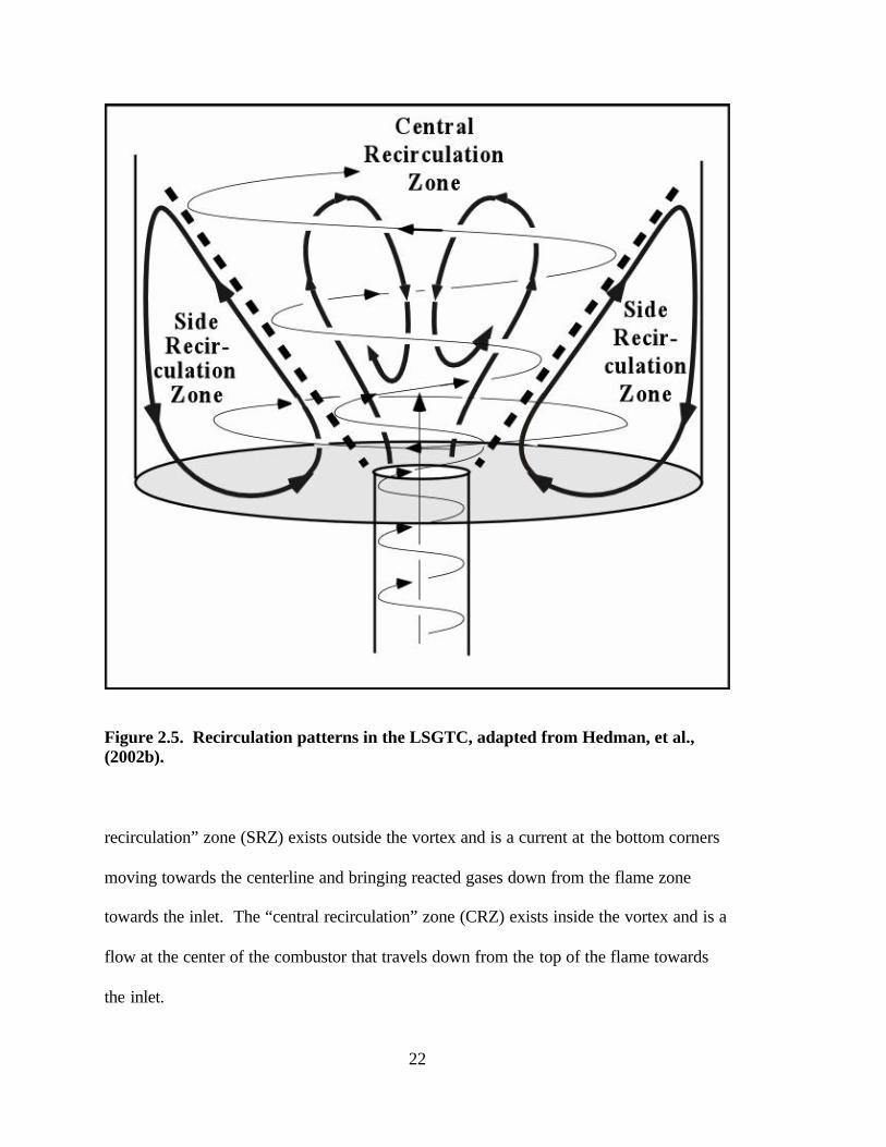
22
Figure 2.5. Recirculation patterns in the LSGTC, adapted from Hedman, et al., (2002b). recirculation” zone (SRZ) exists outside the vortex and is a current at the bottom corners
moving towards the centerline and bringing reacted gases down from the flame zone
towards the inlet. The “central recirculation” zone (CRZ) exists inside the vortex and is a
flow at the center of the combustor that travels down from the top of the flame towards
the inlet.
23
3. THE BYU DUAL DYE SINGLE STOKES CARS INSTRUMENT
3.1 CARS Instrument Description
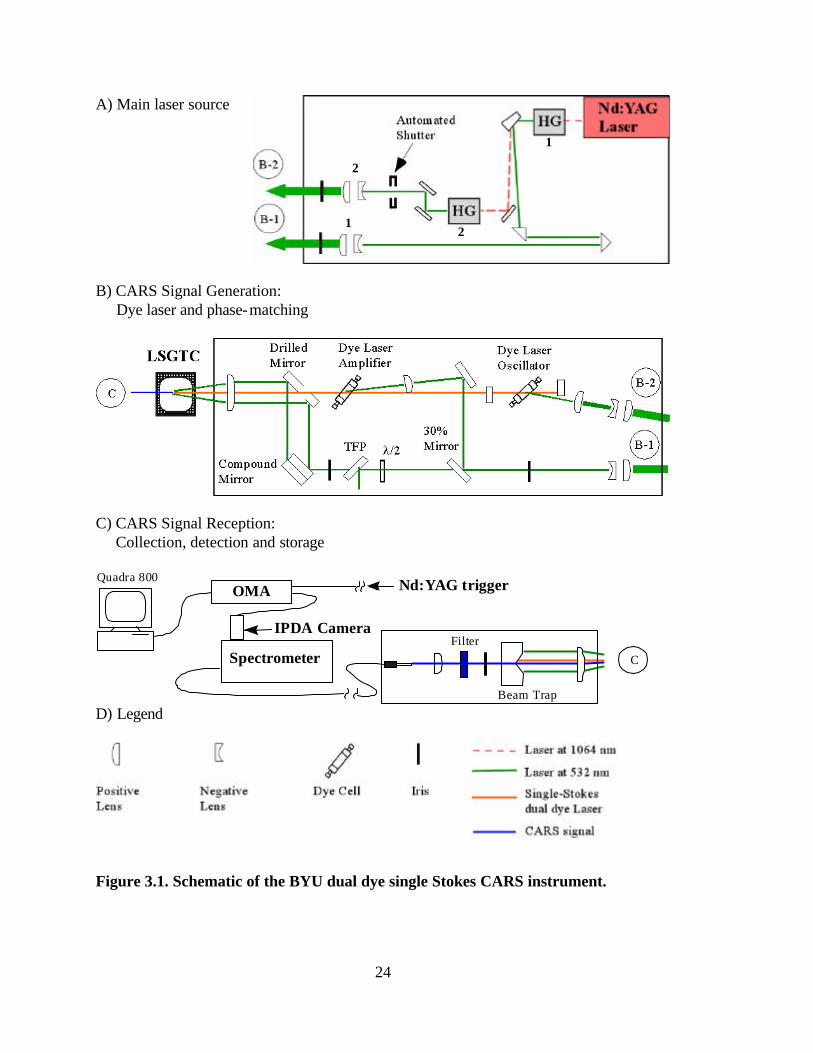
The BYU dual dye single Stokes CARS instrument consists of one laser source and a
collection of several optical and electronic components. The instrument can be
partitioned into three groups as shown in Figure 3.1: A) main laser source; B) CARS
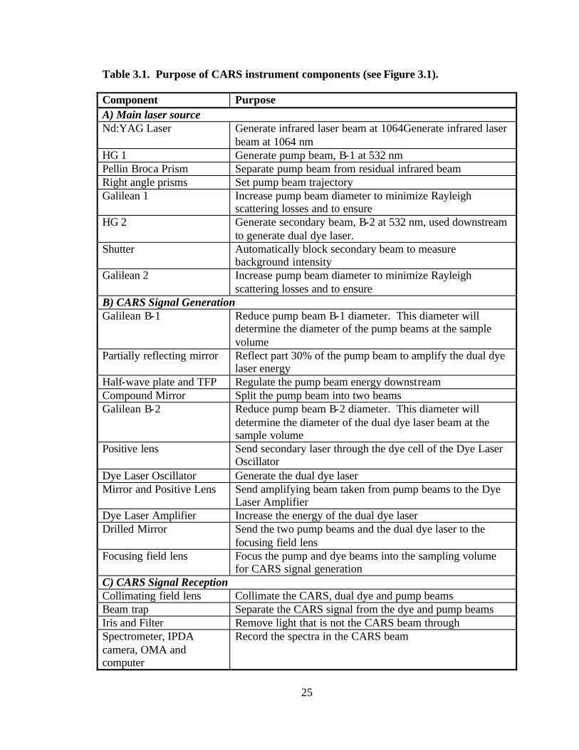
signal generation; and C) CARS signal reception. Each component of the CARS
instrument is described briefly in Table 3.1.
In the main laser source section of the instrument (Figure 3.1A), an Nd:YAG laser
from Quanta-Ray produces an infrared (IR) beam, with a gaussian spatial distribution and
at a wavelength of 1064 nm, which powers all lasers needed to generate the CARS signal.
The Nd:YAG laser was set to operate with the Q-switch turned on at 60 J/pulse on the
oscillator and 50 J/pulse on the amplifier. This IR laser goes through a harmonic
generator (HG) to generate a linearly p-polarized green laser at a wavelength of 532 nm.
A pellin broca prism is then used to separate the superimposed green and unconverted
IR beams coming out from the HG. After being separated, the green laser energy is 290
mJ/pulse whereas the IR beam energy is 212 mJ/pulse. This green laser, from here on
referred to as the primary beam, is then redirected towards a Galilean telescope by two
right-angle prisms which are separated by a distance that synchronizes the arrival of the
all the lasers at the sampling location. The Galilean telescope (-50 / +200 mm focal
length lenses) enlarges the primary beam diameter to become the collimated beam B-1.
24
A) Main laser source
B) CARS Signal Generation: Dye laser and phase-matching
C) CARS Signal Reception: Collection, detection and storage
Spectrometer
OMA
IPDA CameraFilter
Beam Trap
Quadra 800
C
Nd:YAG trigger
D) Legend
Figure 3.1. Schematic of the BYU dual dye single Stokes CARS instrument.
1
2
2
1
25
Table 3.1. Purpose of CARS instrument components (see Figure 3.1).
Component Purpose A) Main laser source Nd:YAG Laser Generate infrared laser beam at 1064Generate infrared laser
beam at 1064 nm HG 1 Generate pump beam, B-1 at 532 nm Pellin Broca Prism Separate pump beam from residual infrared beam Right angle prisms Set pump beam trajectory Galilean 1 Increase pump beam diameter to minimize Rayleigh
scattering losses and to ensure HG 2 Generate secondary beam, B-2 at 532 nm, used downstream
to generate dual dye laser. Shutter Automatically block secondary beam to measure
background intensity Galilean 2 Increase pump beam diameter to minimize Rayleigh
scattering losses and to ensure B) CARS Signal Generation Galilean B-1 Reduce pump beam B-1 diameter. This diameter will
determine the diameter of the pump beams at the sample volume
Partially reflecting mirror Reflect part 30% of the pump beam to amplify the dual dye laser energy
Half-wave plate and TFP Regulate the pump beam energy downstream Compound Mirror Split the pump beam into two beams Galilean B-2 Reduce pump beam B-2 diameter. This diameter will
determine the diameter of the dual dye laser beam at the sample volume
Positive lens Send secondary laser through the dye cell of the Dye Laser Oscillator
Dye Laser Oscillator Generate the dual dye laser Mirror and Positive Lens Send amplifying beam taken from pump beams to the Dye
Laser Amplifier Dye Laser Amplifier Increase the energy of the dual dye laser Drilled Mirror Send the two pump beams and the dual dye laser to the
focusing field lens Focusing field lens Focus the pump and dye beams into the sampling volume
for CARS signal generation C) CARS Signal Reception Collimating field lens Collimate the CARS, dual dye and pump beams Beam trap Separate the CARS signal from the dye and pump beams Iris and Filter Remove light that is not the CARS beam through Spectrometer, IPDA camera, OMA and computer
Record the spectra in the CARS beam
26
The residual IR laser coming of the pellin broca prism is reflected by a mirror into a
second HG to produce another linearly p-polarized green laser, the secondary beam,
which is used as the energy source for the dye laser oscillator. The secondary beam is
then redirected towards a secondary Galilean telescope by two mirrors coated for optimal
reflection of 532 nm light—the residual IR light passing through the mirrors being
collected into copper beam traps (not shown).
The shutter before the secondary Galilean telescope is used to automate the
acquisition of background noise (see the “Spectra Preprocessing” section in Chapter 4).
The shutter, which is activated by the instrument computer (see Figure 3.1C), acts as a
switch for the dye laser—when closed, the shutter blocks the secondary green laser and
consequently turns off the dye laser. The Galilean telescope (-50 / +120 mm) enlarges
the secondary beam diameter to become the collimated beam B-2 with 25 mJ/pulse of
energy. Enlarging the primary and secondary beams into B-1 and B-2 minimizes energy
losses due to Rayleigh scattering, while collimating the beams keeps them from diverging
as they travel about 23 feet towards two periscopes (not shown) at the beginning of the
signal generation table (see Figure 3.1B). Each periscope is made of two large right-
angle prisms and raises each beam to the height of the signal generation table.
At the signal generation table (Figure 3.1B), the primary beam B-1 is reduced in size
by a Galilean telescope (+200 / -125 mm) and then taken to a partially-reflecting mirror,
where 30% of the primary beam energy is reflected at a right angle in order to be used on
the dye laser amplifier. The rest of the primary beam continues towards an “optical
throttle”, made up of a half waveplate (λ/2) and a thin film plate (TFP) polarizer, newly
added in this work because it can handle the extra power in the laser (140 mJ/pulse in 10
27
nanoseconds). This optical throttle is used to regulate the amount of energy in the
outgoing primary beam by rejecting varying amounts of energy of the incoming primary
beam.
The energy regulation is accomplished by introducing a degree of s-polarization in
the primary beam by rotating a half waveplate and by using the TFP to reflect away the s-
polarized component of the primary beam towards a beam trap (not shown). Only the p-
polarized component of the primary beam goes through the TFP. Its energy is
determined mainly by how much energy was rejected because it was allocated in the s-
polarized component. The degree of s-polarization introduced in the primary beam is two
times as much as the rotation of the waveplate. For example, a waveplate rotation of 45o
rotates the p-polarized primary beam by 90o, completely s-polarizing the beam.
After the throttle, the primary beam goes towards a compound mirror (as used by
Boyack, 1990), which splits the primary beam into two parallel beams and directs them
towards the drilled mirror. These two parallel beams are now the “pump beams” used to
generate the CARS signal, and their centers are about 1.5 cm apart.
At the beginning of optical table B, the secondary beam B-2 is aimed at an angle
towards the oscillator dye cell, and, on its way, is first reduced in size by a Galilean
telescope (+150 / -50 mm) and then focused past the oscillator dye cell by a positive lens
(+300 mm). About 15 cm after the focusing lens, the secondary beam passes through the
oscillator dye cell, generating the broadband dye laser. The cell is tilted near the
Brewster's angle relative to the dye laser in order to maximize p-polarized laser output.
The dye laser cavity is enclosed by two flat mirrors coated for reflection of broadband
light centered at 589 nm—a fully-reflecting mirror and a 50% reflecting mirror, each
28
about 10.8 cm apart from the dye cell. The residual secondary beam laser is contained in
a copper trap, whereas the dye laser is directed towards the amplifier cell which is also
tilted at near the Brewster’s angle.
At the amplifier cell, the dye laser power is increased from 8 to 45 mJ/pulse energy
by nearly superimposing it with the amplifying green laser (78 mJ/pulse) that was split at
the 30% mirror, redirected by a full mirror and focused past the amplifying cell with a
+700 mm focal length lens. The residual green laser is trapped (not shown), whereas the
amplified dye laser is then enlarged in diameter by a Galilean telescope (-100 / + 177
mm) and passes through the drilled mirror hole (drilled at a 45 o angle). The position of
the positive lens of the Galilean can be adjusted in all three directions at right angles,
which is useful for the fine adjustments required for phase-matching the CARS signal.
At the drilled mirror, the pump lasers are reflected to be in a plane below and parallel
to the dye laser. The centers of the pump lasers are 4.5 cm below the dye laser center to
ensure phase matching for the N2, CO, O2 and CO2. Before the focusing field lens, the
dye beam has 45 mJ/pulse of energy whereas the pump beams maximum available
energies are 52 and 67 mJ/pulse. The three beams then go through the field lens (+300
mm), which focuses them on the sampling diagnostic volume.
The time resolution of the instrument is dictated by the pulse duration and frequency
of the Nd:YAG laser, which in this work were respectively about 10 nanoseconds and 10
Hz. On the other hand, the spatial resolution of the CARS instrument is determined by
the diameter ( D ) of the beams prior to focusing on the diagnostic volume, the focal
length lf of the focusing lens, and the wavelength λ of the beams. The sampling
volume can be approximated as a cylinder of diameter d and length L, both calculated
29
according to Regnier (1974):
Df
πλ
φ4
= (3.1)
λ
π 23 dL = (3.2)
The approximate diameters of the beams right before the field lens are 10 mm for the
dye beam and 13 mm for the pump beams. According to these values, the minimum
dimensions of the diagnostic volume are estimated to be 20 µm in diameter and 1 mm
long.
One significant practical challenge was to minimize the heat transmitted from the
flame to the optics near the burner. Such heat may deform the shape of the lenses and
mirrors of the instrument to the point of misaligning the lasers, and may even damage
these optical components. In this work, two metal heat shields (not shown) were
mounted at the ends of the optical tables near the LSGTC. Each metal shield had one
0.75 in diameter hole to allow passage of the laser beams. Additional cooling for each
field lens was provided by one fan that circulated cool air from the lab into the optical
table B and another fan right next to the field lens.
After the diagnostic volume, the three original beams and the generated CARS signal
beams pass through another positive lens (+350 mm), where they are collimated. A
copper beam trap downstream collects the dye and pump beams, while the CARS signals
pass through an iris that partly blocks scattered green and dye laser light. Any remaining
scattered green and dye laser light is filtered out using a custom made filter (Warren,
1994) that has maximum throughput centered at 475 nm and a bandwidth of 50 ±10 nm at
Full Width Half-Maximum (FWHM). The CARS signals are focused by a positive lens
30
(+100 mm) onto a custom-made fiber optic that has a 250 µm inlet diameter that tapers
down to 50 µm. The fiber optic conducts the CARS signals into the spectrometer (see
Boyack, 1990) where they are optically manipulated for detection and recording.
The CARS signal detection and recording equipment used in this work is the same
previously used by Warren (1994). The spectrometer spreads and focuses the CARS
signal onto the Intensified Photo-Diode Array (IPDA) of a PARC 1421B camera. This
IPDA has 1024 photo-diodes (pixels) evenly distributed over a one- inch long array. Each
pixel measures light intensity in “detector counts”.
The IPDA camera is controlled by an EG & G Optical Multi-channel Analyzer
(OMA) through a 1461 interface (Boyack, 1990). By scanning the IPDA, the OMA
obtains the detector counts detected by each of the 1024 pixels and stores them in arrays
of 1024 elements in its built- in memory, which can hold up to 1000 full IPDA scans. The
IPDA scans are then transferred from the OMA to the computer where they are stored in
a hard drive in ASCII format.
The IPDA was operated at a temperature of –5oC to reduce the amount of background
noise due to thermal excitation of the photo-diodes. For single-shot measurements, the
OMA was set to combine into a single measurement the addition of two consecutive
IPDA scans. This approach, which has previously been validated (see Boyack, 1990;
Anderson, et al., 1986), is warranted because of limitations in the synchronization
capabilities between the OMA and the trigger signal from the Nd:YAG laser output
console.
The OMA has a variety of operational modes and capabilities, including signal
triggering, such as the one used to control the dye laser shutter (see Figure 3.1A). The
31
shutter is activated and controlled via interfacing software in a Quadra 800 Macintosh
computer that communicates with the OMA through a General Purpose Interface Board
(Warren, 1994). Warren integrated the interfacing software into Igor (Wavemetrics,
Inc.), a comprehensive graphics and data analysis software with programming
capabilities, providing a very flexible and convenient interface for data acquisition.
The original Igor Macros used by Warren were significantly modified to meet the
needs of this research (see Appendix A). Two main modifications were made: 1) the
OMA and IPDA camera were operated the same way as outlined by Boyack for each data
acquisition task (see CARS sampling section in the Experimental Program chapter); and
2) an automated procedure was implemented to name the experimental files according to
a convention designed for the data collected in this work.
3.2 The Dual Dye Single Stokes Laser
3.2.1 Development
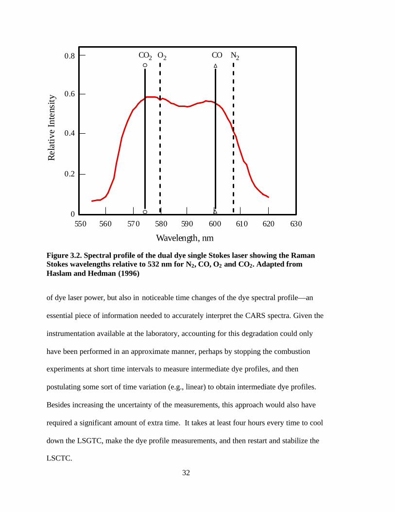
As part of this dissertation work, development was completed for the broadband dye
laser that was first introduced by Haslam and Hedman (1996). This new dye laser is
based on a mixture of two dyes. The spectral energy distribution of the resulting Stokes
allows simultaneous CARS measurements of N2, CO, O2 and CO2. Haslam and Hedman
used two new Pyromethene dyes, P567 and P650, both available from Exciton, Inc.,
dissolved in ethanol. The resulting broadband laser exhibited a bimodal spectral energy
distribution spanning from about 560 nm to 620 nm—covering completely all Stokes
frequencies for N2, CO, O2 and CO2 (see Figure 3.2) relative to a pump beam of 532 nm.
Haslam and Hedman noted that the dye laser degraded within a few hours of use, an
issue that required further investigation. This degradation resulted not only in the decay
32
of dye laser power, but also in noticeable time changes of the dye spectral profile—an
essential piece of information needed to accurately interpret the CARS spectra. Given the
instrumentation available at the laboratory, accounting for this degradation could only
have been performed in an approximate manner, perhaps by stopping the combustion
experiments at short time intervals to measure intermediate dye profiles, and then
postulating some sort of time variation (e.g., linear) to obtain intermediate dye profiles.
Besides increasing the uncertainty of the measurements, this approach would also have
required a significant amount of extra time. It takes at least four hours every time to cool
down the LSGTC, make the dye profile measurements, and then restart and stabilize the
LSCTC.
Figure 3.2. Spectral profile of the dual dye single Stokes laser showing the Raman Stokes wavelengths relative to 532 nm for N2, CO, O2 and CO2. Adapted from Haslam and Hedman (1996)
CO2 O2 N2CO
0
0.2
0.4
0.6
0.8
550 560 570 580 590 600 610 620 630
Wavelength, nm
Rel
ativ
eIn
tens
ity
33
In the course of this research, it was discovered that the rapid decay on the dye laser
was accompanied by degradation in the PVC tubing used to circulate the dye mixture
through the dye cells. It was later found out from tubing manufacturer specifications that
PVC tubing is quickly degraded by ethanol, which explains why the PVC tubing became
noticeably colored within a few hours after replacement. The problem was solved by
using polyethylene tubing instead of PVC tubing. When using the polyethylene tubing,
both the dye laser power and spectral distribution over the areas of interest remained
practically constant throughout 3 to 4 days of continuous dye laser operation of 8 to 12
hours a day.
Another practical issue that needed to be addressed was how to moderate the high
power output of this new broadband dye laser. Too much power in the dye laser can
prevent the acquisition of meaningful measurements. In the BYU CARS instrument, dye
laser powers as high as 100 mJ/pulse have been achieved. This is powerful enough to
damage the quartz windows of the LSCTC and to ionize the air molecules at low
temperatures when focused. In addition, even if there is no ionization, high electric field
intensities can distort the CARS spectra via the Stark effect (Eckbreth, 1996).
In an attempt to lower the dye laser power (Haslam, 1996), changes were made to the
green laser beam used to drive the dye laser oscillator, also referred to as the secondary
beam (see Figure 3.1B, in the CARS Instrument Description section). The changes made
included (a) lowering the secondary beam power with the harmonic generator, and (b)
rotating the polarization of the secondary beam to lower the dye oscillator power
conversion. However, during the course of this work, it was discovered that the rotation
of the secondary beam’s polarization resulted in an elliptically polarized dye laser,
34
generating CARS spectra that cannot be interpreted correctly by available software
(Farrow, 1995). One important requirement of the CARS modeling in the CARS
interpreting software used in this work is that all laser beams in the instrument are
linearly polarized.
In this research, a different approach was taken to control the dye laser power while
keeping the laser linearly polarized. The dye laser power was reduced to about 45
mJ/pulse by lowering the power output of the Nd:YAG laser, while maximizing the
conversion in the secondary beam’s harmonic generator and leaving the secondary beam
p-polarized. The Nd:YAG oscillator gain was set to 60 Joules/pulse while its amplifier
gain was set to 50 Joules/pulse with the Q-switch on.
Using the new laser power control scheme, the dye laser spectral profile for the
mixtures suggested by Haslam and Hedman (see Table 3.2) changed dramatically
towards the red side of the light spectrum; i.e., more of the beam energy was now found
in wavelengths greater than 600 nm. At room temperature, this dye laser spectral profile
generated an almost negligible O2 CARS signal, while increasing the CARS signal for N2
by almost an order of magnitude—which was unacceptable for the purposes of this
research. In order to balance the CARS signal strengths of all four species of interest,
new dye concentrations were developed for this work (see Table 3.2).
The new dye concentrations are the same for both the oscillator and amplifier dye
cells, in contrast to using different concentrations, as reported by Haslam and Hedman.
The mixtures require careful preparation because the spectral profile of this laser is very
sensitive to changes in the concentration of P650 and the amounts involved of P650 are
small. For example, a change of 0.1 mg of P650 (about 5% change in a mixture) causes
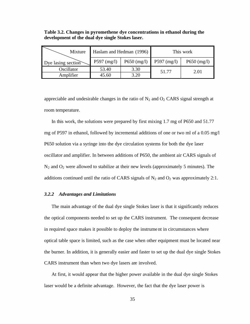
35
appreciable and undesirable changes in the ratio of N2 and O2 CARS signal strength at
room temperature.
In this work, the solutions were prepared by first mixing 1.7 mg of P650 and 51.77
mg of P597 in ethanol, followed by incremental additions of one or two ml of a 0.05 mg/l
P650 solution via a syringe into the dye circulation systems for both the dye laser
oscillator and amplifier. In between additions of P650, the ambient air CARS signals of
N2 and O2 were allowed to stabilize at their new levels (approximately 5 minutes). The
additions continued until the ratio of CARS signals of N2 and O2 was approximately 2:1.
3.2.2 Advantages and Limitations
The main advantage of the dual dye single Stokes laser is that it significantly reduces
the optical components needed to set up the CARS instrument. The consequent decrease
in required space makes it possible to deploy the instrument in circumstances where
optical table space is limited, such as the case when other equipment must be located near
the burner. In addition, it is generally easier and faster to set up the dual dye single Stokes
CARS instrument than when two dye lasers are involved.
At first, it would appear that the higher power available in the dual dye single Stokes
laser would be a definite advantage. However, the fact that the dye laser power is
Table 3.2. Changes in pyromethene dye concentrations in ethanol during the development of the dual dye single Stokes laser.
Haslam and Hedman (1996) This work
Mixture Dye lasing section P597 (mg/l) P650 (mg/l) P597 (mg/l) P650 (mg/l)
Oscillator 53.40 3.30 Amplifier 45.60 3.20
51.77 2.01
36
distributed over such a large spectral range is a limitation in itself because only a small
portion of the laser's energy is actually used in generating the desired CARS signals. In
addition, the total dye laser power can only be raised so much before risking the
introduction of the Stark effect (Eckbreth, 1996).
The dual dye single Stokes laser is also limited by the very fact that it is only one
beam—it cannot be optimally aligned for each of the four species, thus requiring a trade-
off in alignment. As stated earlier in the background section of this dissertation, in order
to generate the CARS signal, it is essential to align the Stokes and pump beams so their
wave vectors satisfy the phase-matching condition. The importance of phase matching is
illustrated by the fact that when maximizing the CARS signals for N2 and CO, the signal
intensities for O2 and CO2 become unacceptably smaller. This alignment trade-off
introduces two limitations: it does not allow taking full advantage of all the energy
available to excite each species, and it restricts where the CARS signals can be focused at
the fiber optic entrance. The latter limitation means that one can be focusing the CARS
signals for N2 and CO near the center of the fiber optic while the CARS signals for O2
and CO2 are closer to the edge of the fiber optic, which may be a problem when beam
steering is present (as explained below).
The limitations introduced by the alignment trade-off required by the dual dye single
Stokes laser presented a practical problem during the acquisition of the combustion data
in the LSGTC. As mentioned earlier, throughout the course of the experiments, the heat
released by the LSCTC, particularly at the hottest locations near the walls, caused small
thermal deformations on the field lenses. This was sufficient to misalign the single
Stokes beam to a degree that warranted realignment during testing.

37
In addition, changes in local density gradients due to flame turbulence seemed to be
causing beam steering, i.e., deviating the path traveled by the CARS signals and
consequently whether they reached the fiber optics entrance. Several CARS spectra had
neither O2 nor CO2 signals. In a premixed natural gas/air system, this is a strong
indication that their CARS signals were steered outside the fiber optic entrance. The
effects of beam steering could be minimized if it were possible to aim both the O2/CO2
signals as well as the N2/CO signals near to the center of the fiber optic entrance.
In conclusion, it is recommended that the performance of the single Stokes instrument
be evaluated in the future against the performance a dual Stokes instrument such as the
one used by Boyack (1990). In particular, if new dyes are identified that offer higher
conversion efficiencies, and therefore more power concentrated in the N2/CO and O2/CO2
spectral ranges, it is possible that a dual Stokes system will perform better than the single
Stokes system. Such a dual Stokes system would deliver more of the Stokes laser energy
into the CARS generation process and it would be possible to maximize all signal
strengths by aligning the N2/CO side independently of the O2/CO2. This alignment
independence would also allow focusing all CARS signals near to the center of the fiber
optic, helping to mitigate (in principle) the effects of beam steering and of lens
deformations due to heating.

38
39
4. CARS SPECTRA INTERPRETATION
Extracting the temperature and species concentrations of each CARS sample obtained
in this work is a complex task. This chapter provides: 1) a description of the numerical
processing performed to prepare each spectrum for interpretation; 2) a brief explanation
of the interpretation procedures used to obtain gas temperature and species
concentrations; and 3) a description of the software developed in order to accomplish the
task of interpreting the large collection of data obtained in this work.
4.1 Spectra Preprocessing
4.1.1 Obtaining the CARS Spectrum from Recorded Spectra
The spectra recorded by the BYU single Stokes CARS instrument, rawI , need to be
preprocessed (i.e., numerically manipulated) before they are ready for interpretation.
Note that rawI stands for all the intensity values in the range of light wavelengths of the
CARS sample. This wavelength dependency is not stated explicitly—a convention of the
field of spectroscopy because the wavelength dependency is “implied” by the nature of
the quantity itself. For clarity, however, the light wavelength dependency of a quantity
will be pointed out whenever the quantity is introduced for the first time in this
dissertation.
Consider the single-shot CARS sample (see Figure 4.1a) obtained in one of the
combustion experiments of this work using the BYU dual dye single Stokes CARS
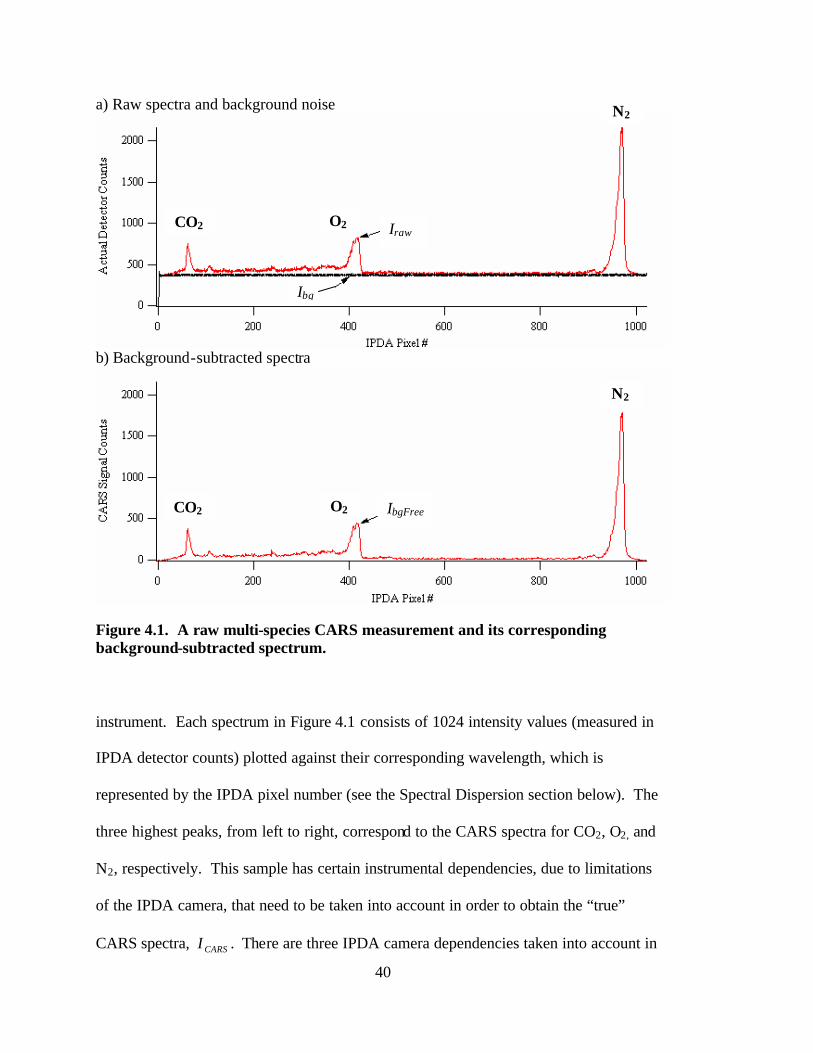
40
a) Raw spectra and background noise
b) Background-subtracted spectra
Figure 4.1. A raw multi-species CARS measurement and its corresponding background-subtracted spectrum. instrument. Each spectrum in Figure 4.1 consists of 1024 intensity values (measured in
IPDA detector counts) plotted against their corresponding wavelength, which is
represented by the IPDA pixel number (see the Spectral Dispersion section below). The
three highest peaks, from left to right, correspond to the CARS spectra for CO2, O2, and
N2, respectively. This sample has certain instrumental dependencies, due to limitations
of the IPDA camera, that need to be taken into account in order to obtain the “true”
CARS spectra, CARSI . There are three IPDA camera dependencies taken into account in
Iraw
Ibg
IbgFree
CO2
CO2
O2
O2
N2
N2

41
this work: background noise, image persistence, and detector non- linearity. Background
noise and detector non- linearity are relevant to both single-shot and average samples,
whereas image persistence is only relevant to single-shot samples.
Background noise originates mainly from the IPDA’s dark current and from any
extraneous light that may arrive on the detector. Dark current arises from charge carriers
produced by heat generated as the IPDA is operated, and thus it exists even in the
absence of light. Although the dark current noise cannot be eliminated, it may be
reduced by operating the IPDA at low temperatures. Thus, in this work, the IPDA was
operated at –5 oC. Other background noise from extraneous light may arrive through the
fiber optic from such sources as scattered laser light from the pump and dye beams, flame
luminosity, or from ambient laboratory light entering the spectrometer.
In the BYU single Stokes CARS instrument, the background noise consists almost
exclusively of the IPDA dark current because practically all extraneous light was kept
from reaching the IPDA. Figure 4.1a shows an averaged sample of background noise
bgI across the wavelength range of the IPDA. This noise exhibits a flat baseline of about
370 detector counts just below the raw CARS signal. The background noise is properly
accounted for by subtracting its intensity values from CARS signal values of
corresponding IPDA pixel as follows
bgrawbgFree III −= (4.1)
The result is a background-free spectral curve bgFreeI , as shown in Figure 4.1b.
4.1.1.1 IPDA Image Persistence
Image persistence is an effect that arises from the limitations of the IPDA and is only
relevant for single-shot samples taken in very short time intervals. Image persistence
42
occurs when a fraction of the light intensity reading in each IPDA pixel for a sample is a
residue from the intensity of a previous sample. The IPDA measures light intensity in
“detector counts”, which are a function of the electric charges generated in each pixel by
the light. After scanning the IPDA to obtain the detector counts in each pixel, the OMA
proceeds to clear the IPDA from the charges. For the time intervals (0.1 seconds)
between each single-shot used in this research, the OMA can only perform seven clearing
scans in between consecutive CARS samples, which are not always enough to completely
clear the charges in each IPDA pixel. Thus, each single-shot sample must be corrected
for the residual intensity left over by the IPDA image persistence.
Boyack (1990) developed the following empirical correlation to estimate the residual
intensity ImaPer in a sample due to image persistence from the previous sample in the
IPDA and OMA system used in this work:
80575.0,, 030095.0)( PrevbgFreePrevbgFree IIImaPer ×= (4.2)
where PrevbgFreeI , stands for the background-free intensity values of the previous single-
shot sample recorded in a given IPDA pixel by the previous sample. The functional
notation )( ,PrevbgFreeIImaPer implies that this correlation is to be used for each of the 1024
intensity readings that make up PrevbgFreeI , . The convenience of this notation will become
apparent later as the use of ImaPer is described.
Boyack’s correlation, Equation 4.2, corrects for the image persistence effect in the
right direction because it subtracts from the current signal a small fraction of the previous
one. It must be noted that the correction is only approximate and somewhat simplistic, as
it cannot account for possible contributions from more than one previous sample.
However, it is considered sufficient because the errors introduced by image persistence
43
are generally small. According to Boyack, the errors in temperature from this effect are
normally less than 50 K, although in extreme cases can reach up to 400 K, while errors
introduced in the species concentrations can be up to 10%.
The degree that image persistence affects a sample depends on the strength of the
intensity of the previous sample relative to the new sample. When the signal intensity of
a previous sample is less than or about the same as the new sample, the residual intensity
will be no more than 1% of the new signal. When the previous signal intensity is
significantly larger, e.g. 5 to 10 times, image persistence effects can account for as much
as 5 to 10% of the new signal. This scenario is particularly possible in turbulent
combustion experiments, where the turbulent variation of gas temperatures can introduce
significant differences in the relative CARS signal strengths of consecutive samples. In
such cases, significant variations of signal strength will occur, because, at low pressures,
the CARS signal strength varies with the square of the sample density (Eckbreth, 1996),
which translates into an inverse variation with the square of the temperature in a gas.
For example, if a sample of a hot gas at 900 K were preceded by a sample of a colder
gas at 400 K, image persistence from the hot gas CARS sample could account by as
much as 6% of the intensity in the cold gas CARS sample. In this case, the expected
error introduced in the temperature could be about 50 K unless the correction factor was
used (Boyack, 1990).
4.1.1.2 IPDA Detector Non-Linearity
Detector non- linearity is another limitation in the capability of the IPDA to quantify
the intensity of the light being measured. The light intensity counts reported by a pixel in
the IPDA are just a fraction of the actual light intensity received, and this fraction varies
44
logarithmically with the intensity of the light being measured, hence the term non-
linearity. This limiting behavior is believed to be common to P-20 phosphor based
detectors (Snelling, et al., 1989) such as the one used in this work.
Equation 4.3 shows a correlation developed by Boyack (1990) quantifying NonLin ,
the non-linearity of the IPDA used in this work:
)ln(04765.060432.0
)(I
IINonLin
+= (4.3)
where I stands for all the background-free intensity values of a single-shot sample
corrected for image persistence from the previous sample as follows:
)vbgFree,PrebgFree ImaPer(III −= (4.4)
Consistent with the definition of Equation 4.2,the functional notation in Equation 4.3
implies that these correlations are to be used for each of the 1024 intensity values in I .
Similarly, Equation 4.4 implies that the image persistence from the previous single-shot
sample measurement in each of the 1024 pixels is subtracted from corresponding pixel
values in the current sample bgFreeI . According to this equation, when a pixel measures
20 counts and below, it is actually detecting only about 70% of the actual light intensity.
This percentage increases logarithmically with detected counts, and at about 4000 counts,
the detector measurement is practically the same as the actual amount of light received by
the pixel.
Detector non- linearity must be accounted for because it has been shown to introduce
significant errors in interpreting CARS spectra unless the spectra are corrected for this
effect. It has been estimated (Boyack, 1990) that errors in temperature values due to non-
linearity vary from 7% at room temperature to 2% at 2000 K, while errors in species
45
concentrations are of the order of 2% or less. These errors are more significant at low
temperatures where peak counts of the CARS spectrum are high. In this case, the
detector non-linearity effects vary significantly throughout the CARS spectrum, being
more noticeable at the wings than at the peak, and the detector non- linearity shrinks the
curve more appreciably. On the other hand, for high temperatures, the peak counts are
usually not much higher than the wing counts, and the detector non- linearity is more or
less even throughout the spectrum, hardly changing the spectrum shape and therefore
introducing only a small amount of error.
The estimated actual CARS spectrum CARSI is obtained from the accumulated
manipulation of the IPDA pixel intensities described by Equations 3.1 through 3.4,
leading to
)( INonLinI CARS = (4.5)
4.1.2 Obtaining the CARS Susceptibility From the CARS Spectrum
After obtaining CARSI , further preprocessing is still required in order to interpret the
CARS measurements. The CARS interpreting software takes as input the CARS
susceptibility, CARSχ , which is essentially a property of the substance being probed. The
susceptibility is embedded in the actual CARS spectra, CARSI , according to the following
relationship (Eckbreth, 1996):
22
CARSdyepumpCARS III χ∝ (4.6)
where pumpI and dyeI are the intensities of the pump and dye lasers, respectively. The
variation with wavelength of pumpI and dyeI is a measurable property of the lasers used in
the experiments and is relatively straightforward to determine. On the other hand,
46
determining the variation of CARSχ with wavelength is not straightforward. First, CARSχ
depends on 21 ωω − , i.e., the difference between the frequencies of the pump and dye
beams, respectively. CARSχ has nonzero values only when 21 ωω − equals a Raman Shift
frequency, Rω∆ , of the molecule of interest. It should also be noted that CARSI intensities
have nonzero values only at frequencies 3ω that equal Rωω ∆+1 . Second, CARSχ values
are different for different Raman transitions of the molecule of interest and vary with
temperature and concentration. Indeed, the measured CARSχ values are the basis by
which the CARS technique can be used to determine temperature and species
concentrations.
In order to extract the CARS susceptibility a dye profile is needed. The dye profile is
the intensity distribution as a function of wavelength of the Stokes laser, in particular
over the spectral range of the CARS spectra of interest. The dye profile is obtained by
taking CARS measurements in a non-resonant gas, i.e., a gas that does not have CARS
transitions where the spectra of the species of interest have. Propane was used as the
non-resonant gas in this work.
Figure 4.2 shows a typical dye profile of the single Stokes dual dye laser. In order to
account for shot-to-shot variations, the dye profile is averaged over several samples. For
this reason, the dye profile is not treated for image persistence but only for background
noise and detector non- linearity, as follows:
)( bgrawDyedyeProfile IINonLinI −= (4.7)
The CARS susceptibility is then obtained from the CARS spectrum by dividing the
dye profile into the CARS spectra and taking the square root of the result as in the

47
Figure 4.2. A sample dye profile from the BYU single Stokes dual dye CARS instrument. following equation:
dyeProfileCARSCARS II∝χ (4.8)
Equation 4.8 assumes that pumpI is exactly monochromatic and therefore a constant.
In reality, however, lasers do have a finite but very narrow spectral width, which is
usually accounted for in the theoretical calculations to obtain accurate CARS spectra
interpretations (see the “Pump Laser Dependency”). However, even in this case,
Equation 4.8 still represents the final numerical manipulation to be performed on the
experimental spectra prior to computational analysis to obtain the temperature and
concentration information from the CARS measurement.
4.2 Accounting for Other Instrumental Dependencies
A CARS spectrum is composed of several peaks of varying intensity at different
wavelengths that originate from each of the rotational and vibrational quantum states that
are populated in the molecule at the time of measurement. Figure 4.3a shows the

48
theoretical CARS spectrum of the N2 at ambient conditions (295 K, 0.85 atm) calculated
using the program CARSFT (Palmer, 1989). On the other hand, the spectra recorded by
the BYU CARS instrument do not show the level of detail of a theoretical spectrum;
instead, each species spectrum is smoothed out into a continuous curve as shown in the
measured N2 CARS spectrum in Figure 4.3b. The spectrum is smoothed out due to a
quantifiable convolution that depends on the specific characteristics of both the
spectrometer and the pump laser, as described in this section.
4.2.1 Spectrometer Dependencies
Two spectrometer characteristics need to be factored into the analysis of the CARS
spectra: the spectral dispersion over the IPDA and the instrument function. Both
characteristics are closely related to each other and are key factors in the final shape a
CARS spectra will have when recorded.
4.2.1.1 Spectral Dispersion
The spectral dispersion is the distribution of light wavelengths focused over the IPDA
pixels and consequently is a measure of the spectrometer resolution. The spectral
dispersion is determined by the holographic grating inside the spectrometer. The spectral
dispersion varies linearly with the distance across the IPDA. Because the pixel centers
are equidistant throughout the IPDA, the distance can be expressed directly in terms of
pixel numbers. Thus, the following expression was used to obtain the spectral dispersion
in terms of wavelength:
( ) 1112
12 λλλ
λ +−
−−
= PPPP ii (4.9)
where iλ is the wavelength in nm reaching the ith IPDA pixel iP (ranging from 1 to
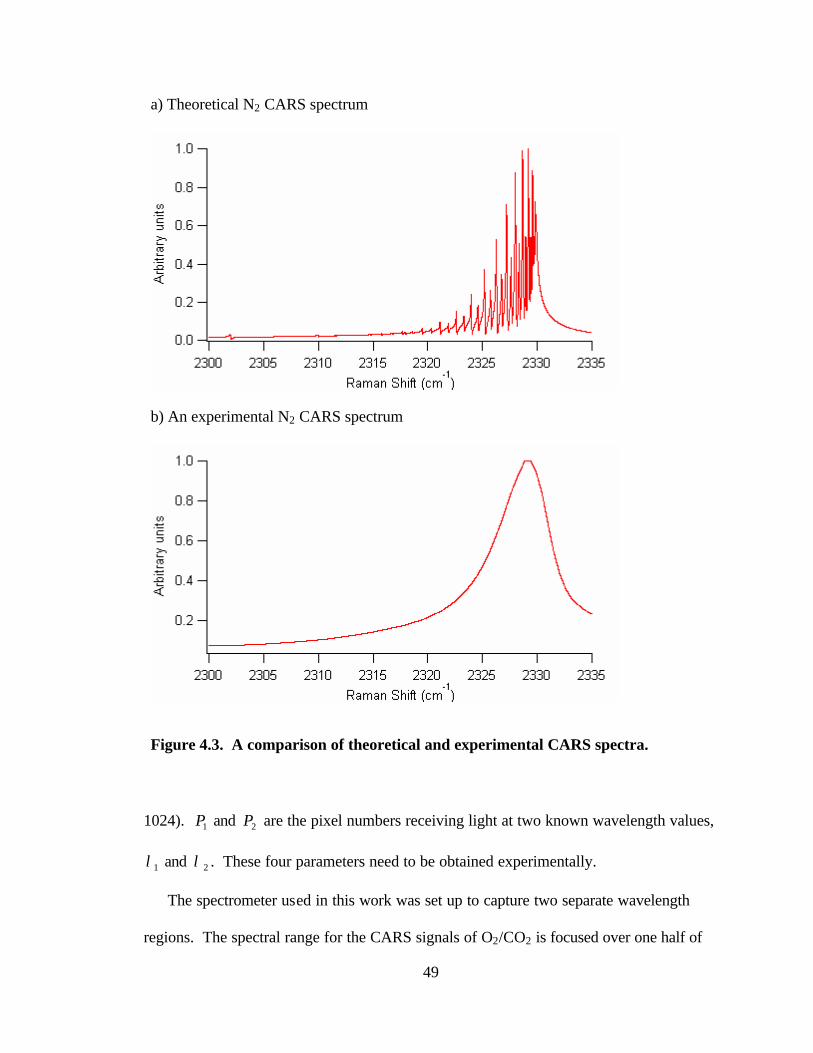
49
a) Theoretical N2 CARS spectrum
b) An experimental N2 CARS spectrum
Figure 4.3. A comparison of theoretical and experimental CARS spectra. 1024). 1P and 2P are the pixel numbers receiving light at two known wavelength values,
1λ and 2λ . These four parameters need to be obtained experimentally.
The spectrometer used in this work was set up to capture two separate wavelength
regions. The spectral range for the CARS signals of O2/CO2 is focused over one half of

50
Figure 4.4. Xenon spectrum obtained by the spectrometer used in this research. the IPDA whereas that for N2/CO is focused over the other half of the IPDA. Therefore,
two spectral dispersions are needed to characterize both sides of the IPDA.
In this work, these spectral dispersions were obtained by measuring the spectrum of a
Xe lamp, which has well-defined spectral peaks at known wavelengths over the spectral
range of interest (see Figure 4.4). The spectral dispersion over the O2/CO2 side is
obtained from the two contiguous peaks at 492.3 and 491.7 nm. The dispersion over the
N2/CO side is obtained using the Xe peaks at 473.4 and 469.7 nm. The Xe peak at 469.7
nm (not shown in Figure 4.4) is about 311 pixels to the right of the 473.4 nm peak. The
separation distance between the 469.7 nm Xe spectral peak and that at 473.4 nm was
measured experimentally by slightly tilting the spectrometer grating to image these peaks
over the IPDA. After this measurement was performed, the grating was tilted back to the
operating configuration in which the 469.7 nm Xe peak is outside the IPDA range.

51
The next step was to express the spectral dispersion in terms of the Raman shift in
wavenumbers, cm-1, the units used in the CARS interpreting codes. The Raman shift
calculated for each pixel is the difference between the frequency corresponding to the
wavelength detected by a given pixel (ω3 from the CARS signal) and the frequency of the
pump beams (ω1). Because λω c= , where c is the speed of light, the Raman shift for
each pixel over the IPDA was calculated in terms of the wavelength the pixel detects as
follows:
7, 10*)532/1/1( −=∆ iiR λω (4.10)
where iR,ω∆ is the Raman Shift in cm-1 at the ith pixel and 532 is the frequency of the
pump beams in nm.
4.2.1.2 Instrument Function
The other spectrometer dependency that needs to be accounted for is the instrument
function, which quantifies how the spectrometer records light at each wavelength. To
illustrate, suppose that a source of monochromatic light of frequency ω0 is available.
Ideally, a spectrometer would measure this monochromatic light as having an intensity
value 0ωI only at the frequency ω0,, i.e., an infinitely narrow line. However, because of
the wavelength nature of light, any spectrometer will record the monochromatic light as
having a distribution of intensities around ω0, with the maximum intensity value 0ωI . If
the spectrometer instrument function were a symmetric Gaussian type, the spectrometer
would broaden the line of the monochromatic light, giving it a “line shape” that would
look like that in Figure 4.5.
In the field of spectroscopy, it is customary to characterize any symmetric line shape
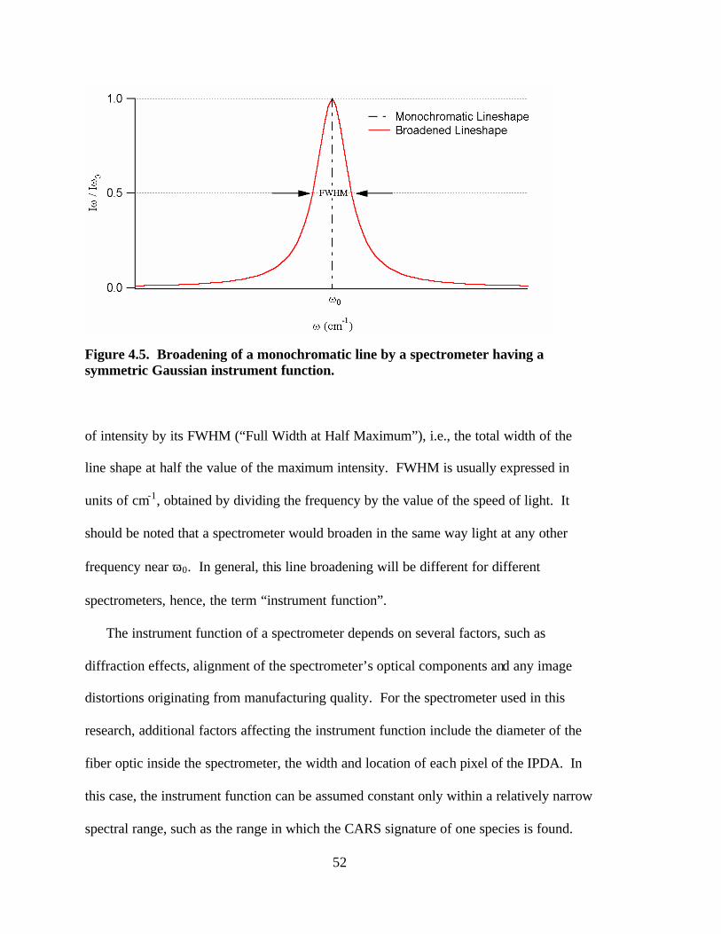
52
Figure 4.5. Broadening of a monochromatic line by a spectrometer having a symmetric Gaussian instrument function. of intensity by its FWHM (“Full Width at Half Maximum”), i.e., the total width of the
line shape at half the value of the maximum intensity. FWHM is usually expressed in
units of cm-1, obtained by dividing the frequency by the value of the speed of light. It
should be noted that a spectrometer would broaden in the same way light at any other
frequency near ω0. In general, this line broadening will be different for different
spectrometers, hence, the term “instrument function”.
The instrument function of a spectrometer depends on several factors, such as
diffraction effects, alignment of the spectrometer’s optical components and any image
distortions originating from manufacturing quality. For the spectrometer used in this
research, additional factors affecting the instrument function include the diameter of the
fiber optic inside the spectrometer, the width and location of each pixel of the IPDA. In
this case, the instrument function can be assumed constant only within a relatively narrow
spectral range, such as the range in which the CARS signature of one species is found.
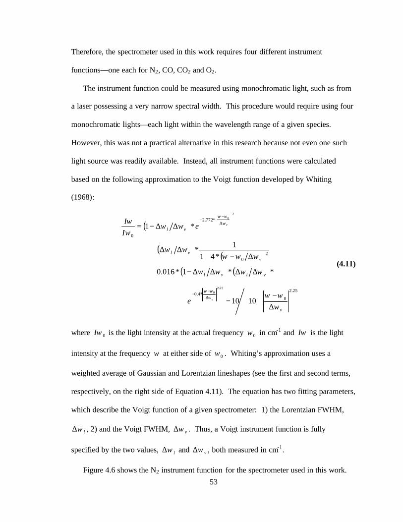
53
Therefore, the spectrometer used in this work requires four different instrument
functions—one each for N2, CO, CO2 and O2.
The instrument function could be measured using monochromatic light, such as from
a laser possessing a very narrow spectral width. This procedure would require using four
monochromatic lights—each light within the wavelength range of a given species.
However, this was not a practical alternative in this research because not even one such
light source was readily available. Instead, all instrument functions were calculated
based on the following approximation to the Voigt function developed by Whiting
(1968):
( )
( )( )
( ) ( )
∆−
+−
∆∆∆∆−+
∆−+∆∆+
∆∆−=
∆−
−
∆−
−
25.2
0*4.0
20
*772.2
0
1010
**1*016.0
*411
*
*1
25.20
20
v
vlvl
vvl
vl
v
v
e
eII
ωωω
ωωωω
ωωωωω
ωωωω
ωωω
ωωω
(4.11)
where 0ωI is the light intensity at the actual frequency 0ω in cm-1 and ωI is the light
intensity at the frequency ω at either side of 0ω . Whiting’s approximation uses a
weighted average of Gaussian and Lorentzian lineshapes (see the first and second terms,
respectively, on the right side of Equation 4.11). The equation has two fitting parameters,
which describe the Voigt function of a given spectrometer: 1) the Lorentzian FWHM,
lω∆ , 2) and the Voigt FWHM, vω∆ . Thus, a Voigt instrument function is fully
specified by the two values, lω∆ and vω∆ , both measured in cm-1.
Figure 4.6 shows the N2 instrument function for the spectrometer used in this work.

54
Figure 4.6. The asymmetric N2 instrument function calculated for the spectrometer used in this research. This is the predicted line shape and width any monochromatic light would appear to have
when measured by the spectrometer of this work in the N2 CARS spectral range. The
frequency in the abscissa is relative to the frequency of interest, i.e., the light at a specific
wavelength. The value of 0ω was arbitrarily set equal to zero in the calculations because
what is needed is the variation in intensity away from any central frequency since the
same instrument function is used throughout the spectral range of the species CARS
signature.
The line shape of the N2 instrument function is slightly asymmetric, and was modeled
by using two Voigt functions, one for the left side of the line shape and another for the
right side (see Table 4.1). Thus, two different sets of values of lω∆ and vω∆ are
required to specify the instrument function of N2, one set for the left side of the line shape
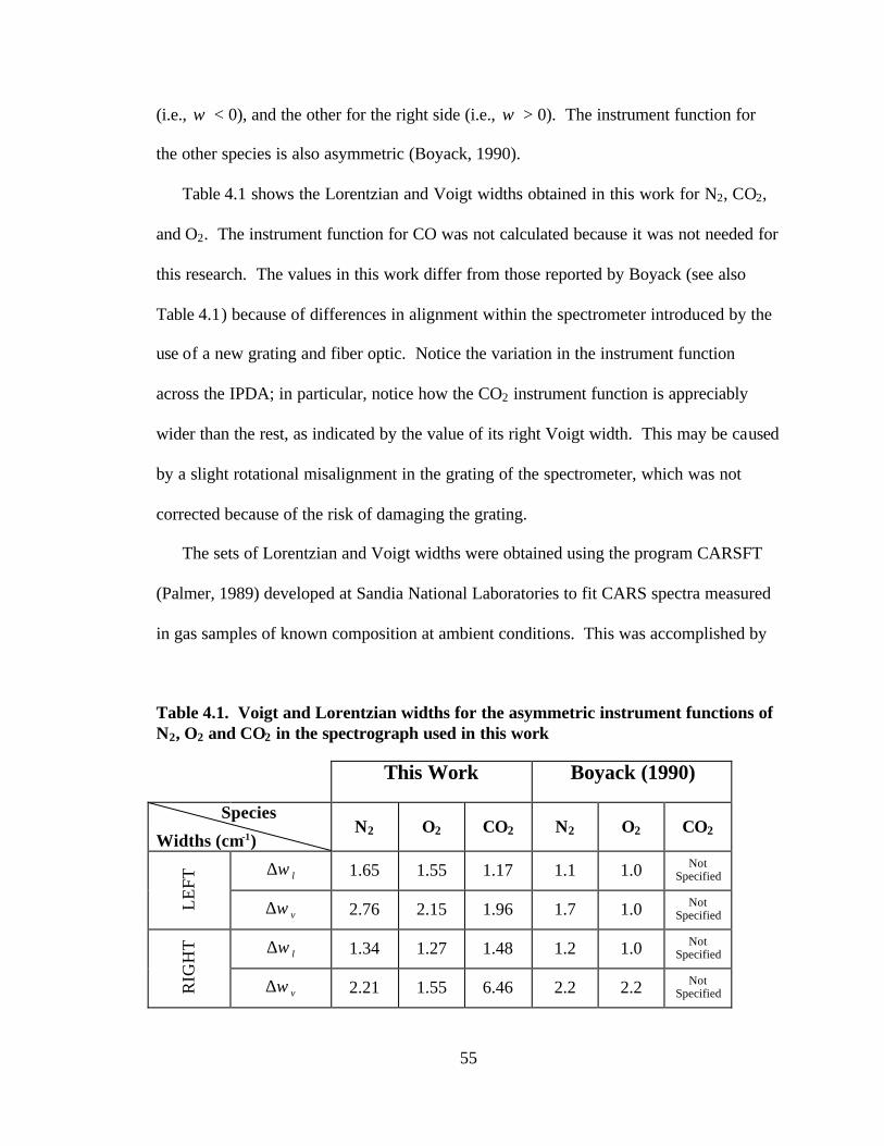
55
(i.e., ω < 0), and the other for the right side (i.e., ω > 0). The instrument function for
the other species is also asymmetric (Boyack, 1990).
Table 4.1 shows the Lorentzian and Voigt widths obtained in this work for N2, CO2,
and O2. The instrument function for CO was not calculated because it was not needed for
this research. The values in this work differ from those reported by Boyack (see also
Table 4.1) because of differences in alignment within the spectrometer introduced by the
use of a new grating and fiber optic. Notice the variation in the instrument function
across the IPDA; in particular, notice how the CO2 instrument function is appreciably
wider than the rest, as indicated by the value of its right Voigt width. This may be caused
by a slight rotational misalignment in the grating of the spectrometer, which was not
corrected because of the risk of damaging the grating.
The sets of Lorentzian and Voigt widths were obtained using the program CARSFT
(Palmer, 1989) developed at Sandia National Laboratories to fit CARS spectra measured
in gas samples of known composition at ambient conditions. This was accomplished by
Table 4.1. Voigt and Lorentzian widths for the asymmetric instrument functions of N2, O2 and CO2 in the spectrograph used in this work
This Work Boyack (1990)
Species
Widths (cm-1) N2 O2 CO2 N2 O2 CO2
lω∆ 1.65 1.55 1.17 1.1 1.0 Not Specified
LE
FT
vω∆ 2.76 2.15 1.96 1.7 1.0 Not Specified
lω∆ 1.34 1.27 1.48 1.2 1.0 Not Specified
RIG
HT
vω∆ 2.21 1.55 6.46 2.2 2.2 Not Specified
56
adding the asymmetric Voigt approximation to the set of analytical functions that
CARSFT could use in performing such spectral fits. The instrument function was
calculated from 0 to 75 cm-1 on each side of the line shape, in increments of 0.1 cm-1.
The FORTRAN code used in implementing the approximation to the Voigt function is
included in Appendix B.
4.2.2 Pump Laser Dependency
The pump laser dependency to be taken into account is the spectral linewidth of the
pump laser itself. The light coming out of our Nd:YAG laser is not exactly
monochromatic but has an intensity distribution centered at 1064 nm, which results in an
intensity distribution centered at 532 nm on the pump laser obtained by frequency
doubling in the Harmonic Generators. Boyack (1990) reported a pump laser linewidth,
FHWM, of 0.51 ± 0.7 cm-1 centered at 532 nm. In this work, the pump laser linewidth
has been assumed to be the same reported by Boyack because the same Nd:YAG and
harmonic generators were used.
The effect of the pump laser linewidth on the CARS signal can be qualitatively
explained by considering the basic requirement to generate a CARS signal for a given
molecular transition: the difference between the frequencies of the pump and Stokes
lasers, 21 ωω − , must match the Raman shift iR,ω∆ for that transition. Thus, when
having a broadband Stokes laser and a pump laser of finite spectral width, the CARS
intensity at each transition results from the all the contributions of each combination of
pump and dye laser frequencies differing by the same Raman Stokes shift.
Taking into account the effects of both the instrument function and pump laser widths
in CARS spectra is not a straightforward matter. The pump laser widths can be

57
accounted for by using either a single (Yuratich, 1979) or a double convolution method
(Teets, 1984; Kataoka, et al., 1982). The latter was the method used in this work.
Additional details on this subject can be found in the CARSFT documentation and
elsewhere in the literature (Palmer, 1989).
4.3 Fitting Methodology
The software used in this work to interpret the CARS spectra is based on a model
proposed by Hall and Boedeker (1984) to fit a theoretical CARS susceptibility
theoryCARS ,χ to its experimental counterpart CARSχ by using temperature and mole fractions
as fitting parameters. The model assumes that the resonant components of theoryCARS ,χ
(Eckbreth, 1996) are dependent on temperature only, and that its total nonresonant
susceptibility component, NRχ , depends only on the mole fractions ix of the mixture
components. Thus, the modulus squared of theoryCARS ,χ for species i can be expressed as
follows:
( ) ( )
( )
+
⋅
⋅+⋅
∝
CARS
CARSNR
iCARS
NR
i
theoryCARS
e
Tfx
Tgx
ω
ωχ
ωχχ
,2,2
2
, (4.12)
where the functions g and f are convolution functions of the resonant components of
theoryCARS ,χ that include the effects of pump laser spectral width and the instrument
function. For broadband Stokes lasers, as is the case in this work, ( )CARSe ω is equal to 1
(Hall and Boedeker, 1984).
58
Equation 4.12 indicates that experimental CARS spectra can be interpreted by fitting
two parameters, namely, the gas temperature T and the ratio ( )NRix χ . The only
requirement is to preprocess the experimental CARS spectra as previously indicated (see
Equations 3.1 through 3.8). The g and f curves are calculated just once for several
temperature values and stored as a set of fitting libraries in a computer hard drive. These
fitting libraries are then used to calculate the theoretical CARS spectra by interpolation
during the fitting process to interpret the experimental CARS spectra. This method is
various orders of magnitude faster to process experimental CARS spectra than the
method of using the detailed CARS spectra calculations (Hall and Boedeker, 1984). The
accuracy of the interpolated functions depends on the interpolation scheme, the proximity
of the temperature values of the g and f curves used for the interpolation, and the mole
fraction values of the species of interest in the sample.
It is important to note that the Sandia developers implemented Hall and Baedeker’s
method in a manner that their library fitting code, FTCARS, uses ( )iNR xχ , i.e., the
inverse of the parameter shown in Equation 4.12. In this work, the program CARSFT
was used to calculate the libraries used by FTCARS for the temperature range of 250 to
2050 K and in increments of 50 K for N2, O2, and CO2. The upper temperature limit was
intentionally set just above the highest adiabatic temperature of the combustion
conditions to be studied. Thus, it is ensured that the CARS fitting methodology was not
bound artificially to only give “reasonable” temperature values.
The instrument functions for each species shown in Table 4.1 were used to generate
their corresponding libraries. These libraries were used to reduce all the data acquired in
this research because the instrument function was found to have remained practically
59
constant throughout the data acquisition period (about three months). This was verified
by using CARS measurements taken on calibration samples for each day that combustion
experiments were performed. The instrument functions were calculated for each daily
sample, showing minor variations. This was particularly true for N2, as confirmed by the
fact that the CARS temperatures obtained using the libraries just mentioned were, within
experimental error, equal to the known temperature values of the daily calibration
samples. Appendix D shows the listing of the input parameters used to calculate the
libraries using CARSFT.
The CARS spectra curve-fitting procedure used in this work is that of the program
FTCARS from Sandia National Laboratories (see more details below). The temperature
and the ratio ( )iNR xχ are the main fitting parameters in a heuristic curve-fitting
methodology to minimize the least squares between the theoryCARS ,χ (obtained by linear
interpolation of the g and f curves) and its experimental counterpart CARSχ (obtained by
pre-processing the experimental CARS measurement).
4.3.1 Computation of Concentrations and Temperature
In principle, the same temperature value should be calculated independently from N2,
O2, and CO2 (Eckbreth, 1996). However, in practice, the accuracy of the temperature
value depends on the accuracy of the CARS spectral characteristics, such as transition
frequency and line wid th, for any given species. Among the species under consideration,
N2 is the best source of temperature measurements because its spectral characteristics are
very well established. In addition, N2 is the most abundant species in the combustion

60
experiments carried out in this work (more than 70 mol-%). Therefore, the gas
temperature for each multi-species CARS sample was taken from the N2 CARS signal.
As mentioned previously, the CARS interpreting technique calculates the
ratio ( )iNR xχ . If the CARS measurement includes all species in a mixture, the mole
fractions can be calculated from the ( )iNR xχ ratios and the relationship 1=∑i
ix .
Otherwise, it is necessary to know either the mole fraction of one of the species or the
value of the total nonresonant susceptibility of the mixture NRχ , which is a mole-fraction
weighted average of the per-molecule nonresonant susceptibilities of the individual
mixture components iNR ,χ , as follows: ( )∑=
iiNRiNR x ,* χχ (4.13)
For the combustion experiments carried out in this work, the abundant quantities of
N2 could provide a simple method of calculating NRχ . Mass balances show that the mole
fraction of N2 remains practically constant from unreacted mixture through total fuel
depletion for the combustion conditions of interest in this work—approximately at 74
mol-% for φ of 0.80 and at 73 mol-% for φ of 0.65. The concentrations of CO and
nitrogen oxides were neglected in the mass balances because they occur in the ppm range
for the combustion conditions in this work (e.g., see Nguyen, et al., 1995; Nandula, et al.,
1996; Cannon, et al., 1999). Therefore, NRχ can be calculated from the N2 CARS mole
fraction and the ratio ( )NRNx χ2 obtained from the N2 CARS spectra. The CO2 and O2
mole fractions follow immediately from the ( )NROx χ2 and ( )NRCOx χ2 ratios obtained
from their respective CARS spectra.
61
4.4 Software Developed in This Work
The CARS spectra interpretation procedure is complex and is compounded even
further when large amounts of data are involved. In this research project, more than one
million multi-species CARS spectra were taken throughout several locations in the
LSGTC for varying combustion conditions, making it essential to devise a means to order
and structure the information.
In this work, a data management system was devised that simplified, automated, and
ensured the proper processing of CARS data through the stages of data acquisition,
interpretation and recording of temperature and species concentrations, and statistical
analysis. The data management system, detailed in Appendix D, starts being
implemented through Igor (Wavemetrics, Inc.) macros programmed to automatically
name the data files stored by the CARS instrument computer in a way that identified the
combustion condition and sampling location where the data were taken.
In addition, a program to Fit Multiple-species Cars Spectra (FMCARS) was written
and used to interpret the spectra taken in this work. FMCARS uses the CARS spectra
interpretation subroutines of the FTCARS program, which accompanies CARSFT
(Palmer, 1989), from Sandia National Laboratories. The FTCARS program was not used
in this research because its interface was not suitable for processing the large number of
acquired measurements. Based on benchmark studies using Hewlett-Packard 780/J-282
UNIX workstations, it would have taken a few years of computer time to process all the
data, plus the time required to prepare the spectra for interpretation by FTCARS and
obtain the desired mole fraction values from the output of FTCARS. On the other hand,
FMCARS can process all the data acquired in this research and output desired parameter
62
values in less than 90 hours of computer time. This considerable reduction in time
requirements was achieved mainly because of an automated and more efficient
processing scheme built into FMCARS.
FMCARS is compatible with the CARS data management system devised in this
work. Appendix B shows a complete listing of the FMCARS code written in this work.
The listing does not include the supporting subroutines used by FTCARS to handle
graphics output and certain mathematical calculations such as interpolation, array sorting,
etc. The FMCARS interface is designed to efficiently process several data files of multi-
species (N2, O2 and CO2) CARS spectra specified by the user through a text file.
FMCARS is also designed to take appropriate actions upon encountering error conditions
of various kinds to ensure continued processing of the specified data files. In the case of
the combustion experiments, each file contains all the samples taken at a combustor
location under a given combustion condition. For each file, FMCARS reads each multi-
species CARS sample in the data files, other required information, handles all
preprocessing and CARS spectra interpretation for each species, and outputs a text file
containing a tabulation of several measurement parameters on a sample-by-sample basis.
The tabulated format facilitates further statistical analysis of the measurement parameters
while properly identifying the location and combustion conditions associated with the
computed statistics. The parameters of each output file are the temperature, non-resonant
susceptibility, O2 and CO2 mole fractions, as well as measurements of curve-fit
“goodness” and spectrum peak detector counts for each species.
In conclusion, the process of extracting temperatures and concentrations from
measured CARS spectra is complex. However, the new software developed in this work

63
facilitated the analysis of the large numbers of experimental samples collected in this
research, while minimizing the risk of human error and making it feasible to reduce all
data within a reasonable amount of time. A summary of the data reduction process as
implemented in the software developed in this work is found in Figure 4.7.
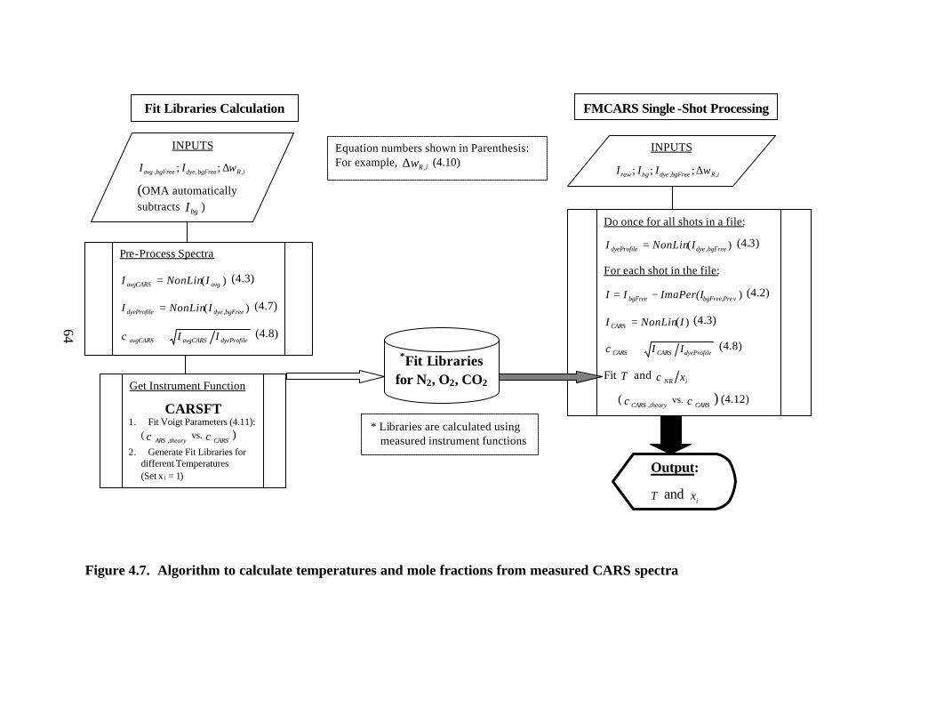
Figure 4.7. Algorithm to calculate temperatures and mole fractions from measured CARS spectra
64
Fit Libraries Calculation FMCARS Single -Shot Processing
Pre-Process Spectra
)( avgavgCARS INonLinI = (4.3)
)( ,bgFreedyedyeProfile INonLinI = (4.7)
dyeProfileavgCARSavgCARS II∝χ (4.8)
Get Instrument Function
CARSFT 1. Fit Voigt Parameters (4.11):
(theoryARS ,χ vs.
CARSχ ) 2. Generate Fit Libraries for
different Temperatures (Set x i = 1)
*Fit Libraries for N2, O2, CO2
Do once for all shots in a file:
)( ,bgFreedyedyeProfile INonLinI = (4.3)
For each shot in the file:
)vbgFree,PrebgFree ImaPer(III −= (4.2)
)(INonLinI CARS = (4.3)
dyeProfileCARSCARS II∝χ (4.8)
Fit T and iNR xχ
(theoryCARS ,χ vs.
CARSχ ) (4.12)
Output:
T and ix
INPUTS
iRbgFreedyebgFreeavg wII ,,, ;; ∆
(OMA automatically subtracts bgI )
INPUTS
iRbgFreedyebgraw wIII ,, ;;; ∆ Equation numbers shown in Parenthesis: For example, iRw ,∆ (4.10)
* Libraries are calculated using measured instrument functions
65
5. ACCURACY AND PRECISION OF THE BYU SINGLE-STOKES DUAL DYE
CARS INSTRUMENT
This chapter describes how the accuracy and precision were estimated for the
measurements obtained using the dual dye single-Stokes CARS instrument. This
treatment is only presented for the temperatures, and the concentrations of O2 and CO2.
The accuracy and precision for the CO concentrations was not pursued because the
CARS instrument did not detect CO during the combustion experiments due to the CO
concentrations being too small to be detected.
5.1 Temperature
The accuracy and precision of the temperatures measured by the single-Stokes CARS
instrument was estimated by collecting CARS measurements of air at atmospheric
pressure at 12 different temperatures in the range of 294 to 1428 K. For each temperature
condition, 1000 CARS samples were collected. The temperature variation was obtained
by using an electrically heated tube furnace from Thermodyne (Type 21100). The
furnace consisted of a cylindrical cavity two inches in diameter and 14 5/8 inches tall,
open to the ambient atmosphere. The furnace temperature readings were obtained using a
type K thermocouple, placed in the middle of the cavity and connected to a digital reader
(Model DP900) from Omega.
Because the furnace was open to the atmosphere, care was taken to keep any
laboratory air streams from entering the furnace during the experiments. In addition, the

66
CARS measurements were taken only when the furnace temperature reading remained
stable for at least two minutes.
As these CARS spectra were reduced, a set of sieving criteria was devised in order to
discard those measurements that were definitely bad, i.e., spectra whose signals were
severely distorted by noise. These sieving criteria were obtained after careful
examination of several CARS spectra. During the examination process, a parameter to
indicate the “goodness” of the fit of theory to experiment was found to be useful for
sieving out bad data. This parameter is the value of the ratio of the area under the
theoretical curve divided by the area under the experimental data curve: experimtheory AA .
This ratio has the advantage that good fits have experimtheory AA ratios close to unity.
During the statistical analysis of the data, the following constraints were
implemented.
1. Discard N2 measurements where the experimtheory AA ratio was less than 0.98 or
greater than 1.2. The upper limit of 1.2 was chosen because some spectra
with appreciable experimental noise yielded reasonable temperature values
while having a experimtheory AA ratio of 1.2. It should be mentioned, however,
that most experimtheory AA values were very close to 1 (see data in the
accompanying CD).
2. Discard N2 measurements where the temperatures were less than 250 K or
greater than 2050 K. It should be mentioned that none of the CARS
measurements in this validation study had temperature values higher than
approximately 1500 K.
67
3. Discard those spectra whose temperature values were more than four times the
standard deviation on either side of the mean CARS temperature.
All the statistical data presented in this work were calculated using only those
measurements that passed the aforementioned sieving criteria.
Table 5.1 shows a comparative analysis between the temperatures measured by the
furnace thermocouple (TFurnace) and the temperatures measured using the BYU single-
Stokes dual-dye CARS instrument. The statistics calculated on the CARS measurements
include the average temperature (<TCARS>) and the standard deviation (σTcars) of
approximately 900 samples at each temperature. The mean CARS temperatures from this
dataset are about 4.6% on average higher than the temperatures obtained by the furnace
thermocouple. The fact that all the CARS average temperatures are higher than their
thermocouple counterparts may indicate the presence of a small systematic error in either
the thermocouple or the CARS measurements.
In order to quantify the precision of the CARS instrument, it was decided to define
the instrument error to be twice the value of the standard deviation. The average error
from the CARS-measured temperatures was ±15.6% in the temperature range from 294
to 1023 K. On the other hand, the error for the higher temperature range from 1175 to
1428 K was 28.2%, about twice as much as from the lower temperature range.
Figure 5.1 shows an alternate presentation of the data contained in Table 5.1. The
empty circles represent the point defined by corresponding pairs of TFurnace and <TCARS>.
The error bars are ±2*σTcars. The dashed line has a slope of one, and therefore represents
the line where all (<TCARS>) would lay on if they were exactly equal to TFurnace. The data
discussed herein suggests that the temperature accuracy of the BYU dual dye single
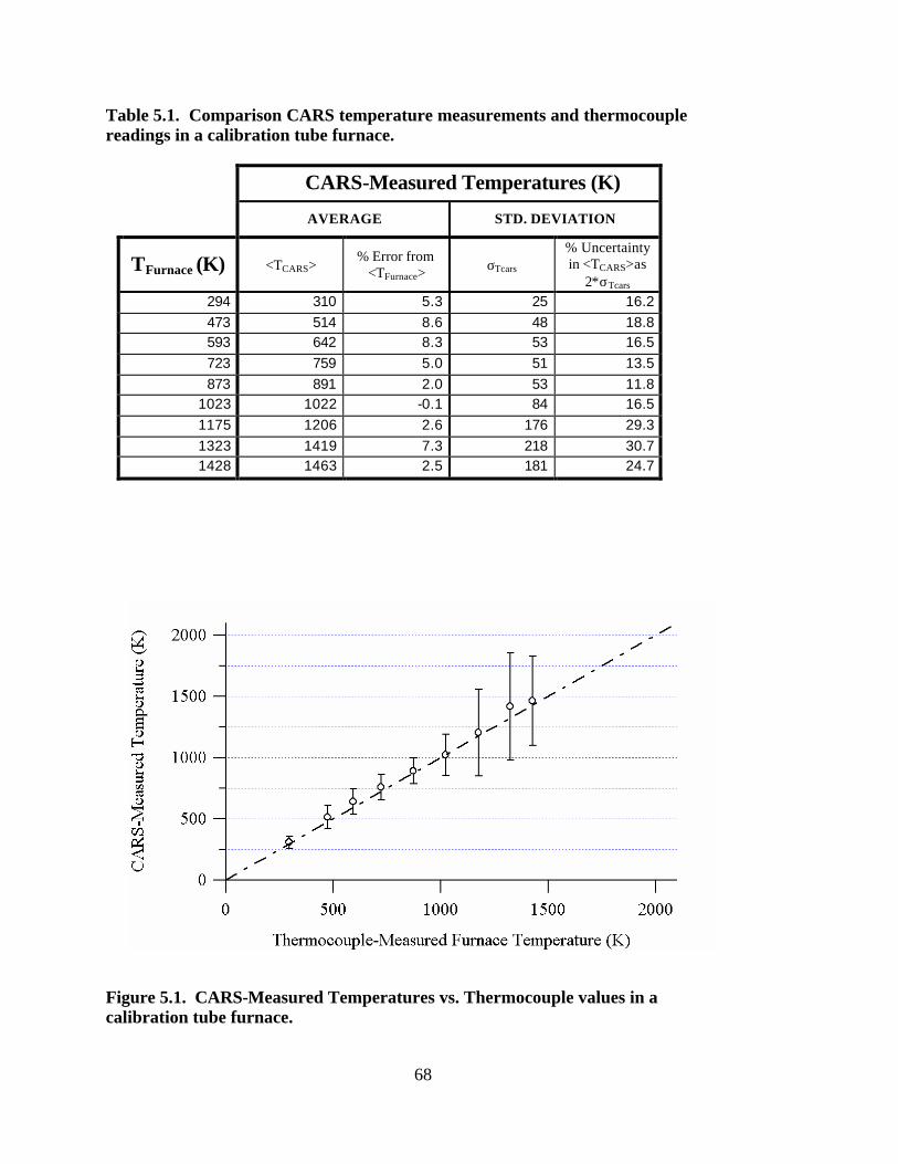
68
Table 5.1. Comparison CARS temperature measurements and thermocouple readings in a calibration tube furnace.
CARS-Measured Temperatures (K)
AVERAGE STD. DEVIATION
TFurnace (K) <TCARS> % Error from
<TFurnace> σTcars
% Uncertainty in <TCARS>as
2*σTcars
294 310 5.3 25 16.2 473 514 8.6 48 18.8 593 642 8.3 53 16.5 723 759 5.0 51 13.5 873 891 2.0 53 11.8
1023 1022 -0.1 84 16.5 1175 1206 2.6 176 29.3 1323 1419 7.3 218 30.7 1428 1463 2.5 181 24.7
Figure 5.1. CARS-Measured Temperatures vs. Thermocouple values in a calibration tube furnace.
69
Stokes CARS instrument is good any where between 300 and 1428 K. The data also
suggest that the instrument’s precision for temperature is acceptable, particularly below
1200 K. For temperatures higher than 1200 K, the data seem to suggest that the
instrument’s precision is only fair. However, the analysis that follows supports the
possibility that the data for the three highest temperature conditions in the furnace are
suspect, not due to instrumental limitations, but due to experimental difficulties
encountered only in these calibration experiments.
Figure 5.1 shows the probability density function (or PDF) for each of the
temperature conditions measured in the furnace. Each PDF was calculated after sieving
the corresponding 1000 CARS samples, as specified previously. The temperature value
found in the legend box inside each graph is the thermocouple temperature, TFurnace. Note
that the temperature distribution at 294 K is almost a straight line, showing that variations
from the mean are not very significant at this condition. For the temperatures between
473 and 1023 K, the probability density functions of temperature follow a normal
distribution. However, the probability density functions for 1175, 1323, and 1428 K do
not follow a normal distribution. Instead, their distributions consistently follow the same
pattern, having a stretched tail down to lower temperatures.
It is possible that the lower temperature values resulted from “faint” CARS samples,
i.e., those with very low detector counts. In those cases, a CARS spectrum could be
significantly distorted, or even worse, not detected at all, resulting in lower temperatures
than actually measured. In order to substantiate this idea, the FMCARS output files for
the three temperature conditions in question were analyzed. The analysis focused on the
following values obtained from each individual N2 spectrum: 1) the fitted temperature
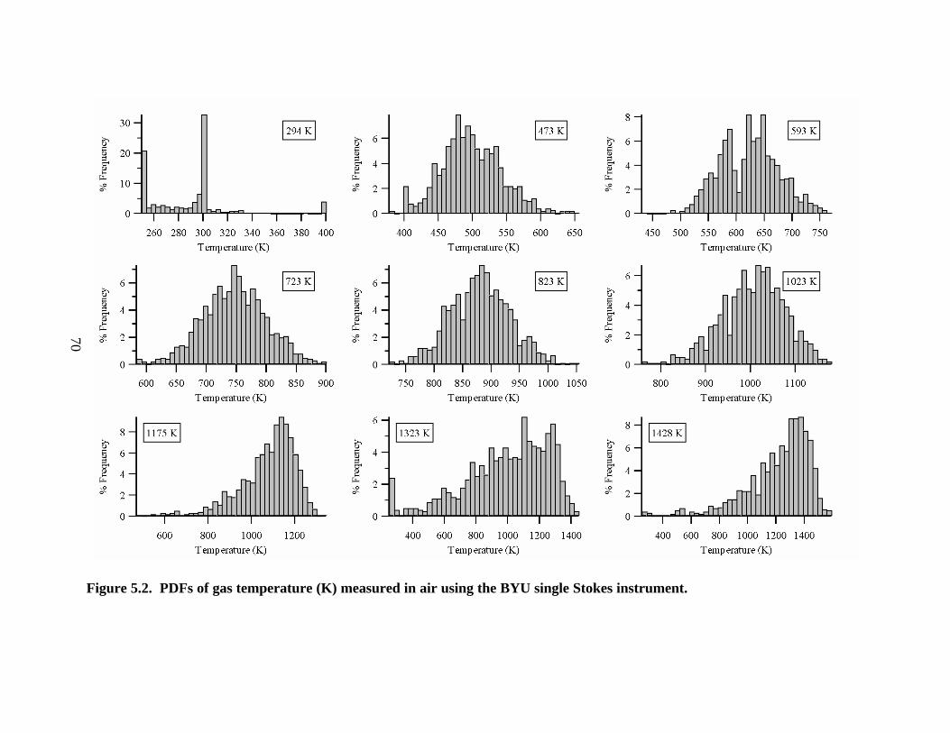
Figure 5.2. PDFs of gas temperature (K) measured in air using the BYU single Stokes instrument.
70

71
value, and 2) the “peak detector counts”, i.e., the value of the maximum number of counts
recorded by the detector for the given spectrum. Using Microsoft Excel, new average
and standard deviations were calculated by including only those spectra with peak
detector counts greater than or equal to 80. This number was empirically chosen after
visual inspection of several FMCARS fits of CARS N2 spectra having a wide range of
peak detector counts.
Table 5.2 shows the <TCARS> and σTcars obtained when discarding all N2 spectra with
peak counts less than 80. The average temperatures did not change significantly. On the
other hand, the standard deviations were reduced by about a third from the values
reported in Table 5.1 resulting in an average error of 13.8% for the three temperature
conditions. Note that a significant number of CARS samples had peak counts less than
80, for example, 60% of the samples taken at 1428 K were discarded based on this
criterion.
This analysis provides evidence that supports the idea that large errors reported at
temperatures greater than 1200 K do not necessarily reflect the precision of the
instrument, but rather may be caused by experimental difficulties in obtaining strong
Table 5.2. Empirically corrected CARS temperature measurements vs. thermocouple readings in a calibration tube furnace.
CARS-Measured Temperatures (K)
AVERAGE STD. DEVIATION
TFurnace (K) <TCARS> % Error from
<TFurnace> σTcars
% Uncertainty in <TCARS>as
2*σTcars
# of Kept Shots
1175 1118 -4.8 88 15.0 728 1323 1249 -5.6 93 14.0 237 1428 1373 -3.9 89 12.5 400
72
enough CARS signals. Possible sources of these experimental difficulties include, but
may not be limited to, the following: (1) loss in dye laser power due to random intensity
and dye profile variations, and (2) misalignment of the pump and dye lasers due to the
intense heat originating from the tube furnace that introduced slight expansion in the
focusing lenses. It is believed that the latter was the most important factor because the
focusing lenses were not shielded during these experiments due to the tube furnace size,
and because the lasers had to be realigned every time the CARS sampling was started for
each of the high temperature cases due to loss of CARS signal intensity.
The aforementioned analysis raises the question whether the CARS spectra whose
peak counts are less than 80 should be discarded during the analysis of the combustion
cases investigated in this work. However, this approach was decided against because of
its potential negative impact in the analysis of samples taken in flame regions with very
large temperature variations. For example, several valid samples might be discarded in
regions where intense turbulent mixing of hot and cold gases with large temperature
differences occurs—a situation that was observed in several locations for all combustion
cases during the experiments. In these cases, the CARS instrument power had to be low
enough to not ionize the cold gases, yet high enough to detect the hotter ones. Thus, hot
gases may end up yielding lower-count spectra that are still of good quality and can give
valid information.
Based on the preceding analysis, it is postulated that the actual uncertainty in the
temperature data collected in the combustion experiments of this research is about ±15%,
throughout all the temperature range, because the CARS instrument optics were
adequately shielded from the heat released by the combustion system under study.
73
5.2 O2 Concentrations
The accuracy and precision of the O2 measurements for the new BYU CARS
instrument were studied using the data collected in the same experiments used for the
temperature analysis. These O2 spectra were also sieved according to the following
criteria:
1. Discard O2 spectra whose companion N2 spectra were discarded in the
temperature analysis.
2. Discard the O2 measurements where the ratio experimtheory AA was less than
0.98 or greater than 1.2. The upper limit was chosen to be consistent with
the N2 sieving criteria.
3. Discard those spectra whose O2 mole fractions were more than four times
the standard deviation at either side of the mean.
4. Any N2 spectrum meeting the sieving criteria described in section 1 of this
chapter was kept even if its companion O2 spectrum was discarded
because the temperature value from the N2 spectrum is still valid.
The temperature value for each O2 spectrum was set to be the temperature value of its
companion N2 spectrum. In addition, FMCARS was modified to output the
concentrations ratio 22 NO xx from the companion fit parameters NROx χ2 and NRNx χ2
for each CARS sample. Thus, the N2 and O2 mole fractions can be calculated directly in
these validation experiments by neglecting the other minor components in ambient air,
i.e., assuming that 122 =+ NO xx .
Table 5.3 shows the average and standard deviations obtained for the sieved O2
CARS calibration samples at each temperature condition. Also shown are the % error

74
Table 5.3. CARS O2 concentration measurements in a calibration tube furnace. Air was used in the furnace; therefore, the actual O2 mole fraction was 0.21.
CARS-Measured O2 mole fractions
AVERAGE STD. DEVIATION
TFurnace (K) <XO2> % Error from 0.21 (XO2 in
air) σ XO2
% Uncertainty as 2*σXO2
294 0.207 -1.6 0.033 32.3 473 0.201 -4.4 0.026 25.5 593 0.192 -8.6 0.026 26.8 723 0.184 -12.6 0.025 27.2 873 0.178 -15.1 0.023 26.0
1023 0.178 -15.3 0.028 31.9 1175 0.194 -7.9 0.046 47.7 1323 0.261 24.3 0.081 62.1 1428 0.235 12.0 0.074 62.7
and the % uncertainty. The % error is a measure of the accuracy of the CARS instrument
and was defined as the % difference between the measured average mole, <XO2>, and
0.21, the mole fraction of O2 in air. From 294 to 1023 K, the <XO2> values are slightly
lower than the actual O2 concentration. In this temperature range, the % error increased
with temperature from 1.6% at 294 K to about 15% at 1023 K. For the three highest
temperatures, there is no apparent trend in the variation of % error. However, with the
exception of the data at 1323 K, the % error is still within 15%.
The % uncertainty (shown in Table 5.3) is a measure of the precision of the BYU
single-Stokes CARS instrument and was defined as ± two times the standard deviation of
<XO2> expressed as a percent error. From 294 to 1023 K, the uncertainty in the
concentration is about 30% higher or lower than the measured value. For the three
highest temperatures, the uncertainty is even higher—about 60%. The calibration
measurements show that the lowest uncertainty is ± 0.05 mole fraction, a total error bar

75
of 0.1 mole fraction. The uncertainty encompasses about two-thirds of the range of O2
concentrations expected in the combustor (0.19 down to 0.05). It should be pointed out
that the uncertainties are expected to increase for lower O2 mole fraction due to the
interference of the resonant components of other species present in the mixture. In
conclusion, the uncertainty in O2 concentrations is large enough to say that this
implementation is not well suited for the combustor.
Two potential sources have been identified to explain the large concentration
uncertainties, and possible solutions are proposed. The verification and implementation
of these solutions are beyond the scope of this work, but they are thought to be worthy of
pursuit in future research.
The foremost potential source of uncertainty in O2 concentrations is an inherent
limitation in the approximate CARS interpretation method of Hall and Boedeker. This
method has been shown to give large errors in the mole fractions in mixtures where there
are large concentrations of species other than the one being measured (Palmer, 1989; Hall
and Boedeker, 1984), as is the case in both (a) these O2 measurements and (b) in the
combustion experiments, where N2 accounts for more than 70% of the mixture.
These problems could be avoided by analyzing the CARS spectra using the complete
numerical computations found in CARSFT. If it can be shown that there is significant
improvement in the concentration values when using CARSFT, one could modify
FMCARS to use the CARSFT subroutines instead of the library-based procedure of
FTCARS, which uses Hall and Baedeker’s method. This would be a very involved and
potentially time consuming effort. In addition, the resulting code is expected to be very
computationally intensive. Its application to reducing the large amount of experimental
76
data obtained in this work may be prohibitive with current computer technology.
Another alternative to consider is developing another simplification to the CARS
computations that is fit for multi-species concentration measurements. Again, both
approaches to enhancing the accuracy of obtaining species concentrations from the
CARS measurements are beyond the scope of this work.
The second potential source of the large concentration uncertainty is the random
variations in the dye profile of the BYU single-Stokes CARS instrument. The dye profile
variations arise naturally as part of the dye laser generation process and their effects in
single-pulse precision are very complicated to quantify (Eckbreth, 1996). It should be
noted that the FTCARS algorithm already includes a correction procedure suggested by
Snelling (1987) applicable when using an averaged dye profile. This limitation is
inherent to the instrument and can only be addressed by finding either new dyes or dye
laser generation methods with more repeatable laser output.
In conclusion, the large uncertainty of the measurements in the controlled tube
furnace environment raise questions as to the suitability of the new BYU CARS
instrument to measure the O2 concentrations in the turbulent environment of the
combustion cases studied in this work. Because the uncertainties are so large and are
expected to increase for low concentration ranges of O2, it would not be clear whether
any observed variations of O2 concentrations were caused by the flame turbulence or
were an artifact of either the reduction method or the instrument itself. Thus, the analysis
of the O2 concentrations of the combustion cases has been deferred to future work.

77
5.3 CO2 Concentrations
Separate experiments were carried out to determine the BYU CARS instrument
accuracy and precision for the CO2 measurements. A vendor-prepared mixture of 10
mol-%, CO2, 15mol-% CO and 75 mol-% N2 was flowed through a custom-made cell
with optical access for the CARS lasers. The cell was made of clear plastic pipe with an
internal diameter of nearly 6 cm and a length of about 15 cm. Quartz windows were
attached to either end of the pipe and sealed. Two fittings were attached in holes drilled
on the pipe at either end. One fitting was used to attach tubing coming from the mixture
tank, while the other fitting let the mixture flow out of the cell and into the ventilation
hood above the cell. Care was taken to establish the lowest possible flow that would
flush the cell without pressurizing it. The cell was considered flushed, and therefore
filled with the CO2/CO/N2 mixture, when the CARS instrument did not detect any O2.
One thousand samples were taken at room temperature in this experiment.
The 1000 samples were reduced using FMCARS and subsequently sieved using the
same criteria applied for O2. The average measured CO2 mole fraction was 0.49 (as
opposed to 0.1) with a standard deviation of 0.30. Once again, by defining the
uncertainty as two times the standard deviation, the CO2 mole fraction thus obtained
could be anywhere in the range of –0.11 and 1.09, which values are physically
impossible. This leads to the conclusion that the CARS measured CO2 mole fractions are
not reliable.
Further investigation of CO2 CARS spectra reduction revealed that FMCARS fits
resulted in several widely different mole concentrations depending on the initial guess.
For example, when working with the average CO2 spectrum from all the experimental
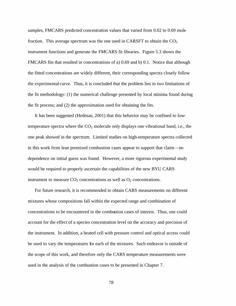
78
samples, FMCARS predicted concentration values that varied from 0.02 to 0.69 mole
fraction. This average spectrum was the one used in CARSFT to obtain the CO2
instrument functions and generate the FMCARS fit libraries. Figure 5.3 shows the
FMCARS fits that resulted in concentrations of a) 0.69 and b) 0.1. Notice that although
the fitted concentrations are widely different, their corresponding spectra closely follow
the experimental curve. Thus, it is concluded that the problem lies in two limitations of
the fit methodology: (1) the numerical challenge presented by local minima found during
the fit process; and (2) the approximation used for obtaining the fits.
It has been suggested (Hedman, 2001) that this behavior may be confined to low-
temperature spectra where the CO2 molecule only displays one vibrational band, i.e., the
one peak showed in the spectrum. Limited studies on high-temperature spectra collected
in this work from lean premixed combustion cases appear to support that claim—no
dependence on initial guess was found. However, a more rigorous experimental study
would be required to properly ascertain the capabilities of the new BYU CARS
instrument to measure CO2 concentrations as well as O2 concentrations.
For future research, it is recommended to obtain CARS measurements on different
mixtures whose compositions fall within the expected range and combination of
concentrations to be encountered in the combustion cases of interest. Thus, one could
account for the effect of a species concentration level on the accuracy and precision of
the instrument. In addition, a heated cell with pressure control and optical access could
be used to vary the temperatures for each of the mixtures. Such endeavor is outside of
the scope of this work, and therefore only the CARS temperature measurements were
used in the analysis of the combustion cases to be presented in Chapter 7.
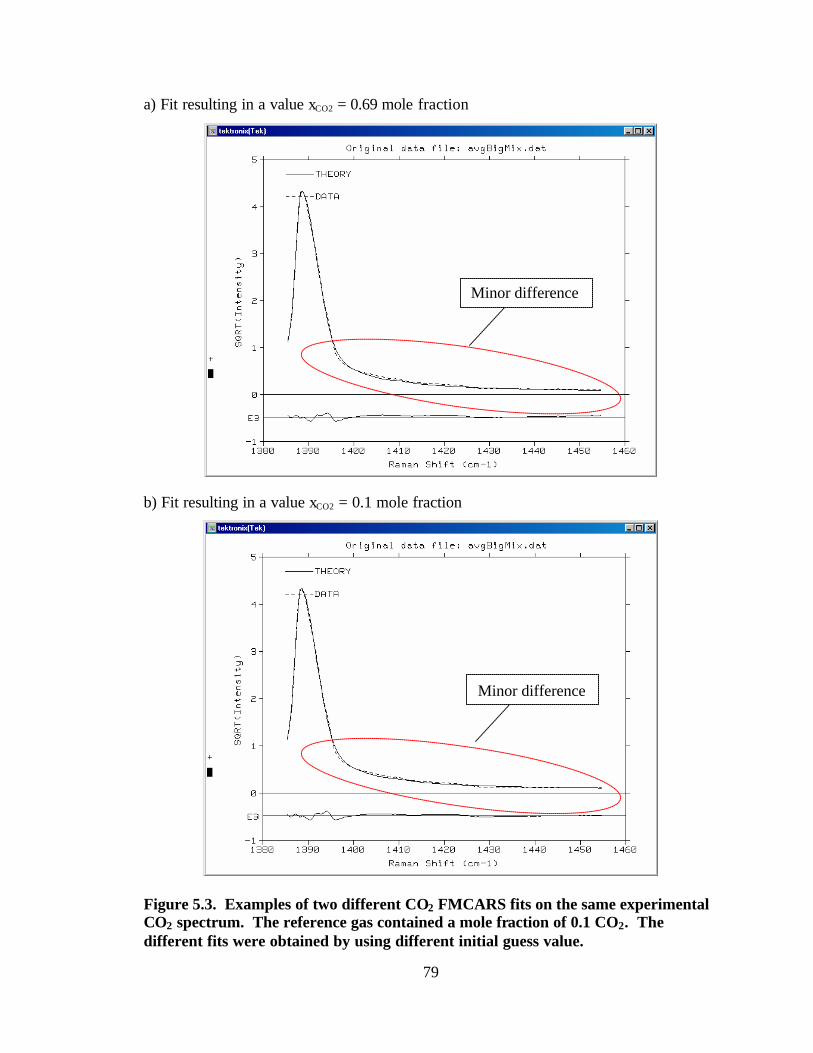
79
a) Fit resulting in a value xCO2 = 0.69 mole fraction
b) Fit resulting in a value xCO2 = 0.1 mole fraction
Figure 5.3. Examples of two different CO2 FMCARS fits on the same experimental CO2 spectrum. The reference gas contained a mole fraction of 0.1 CO2. The different fits were obtained by using different initial guess value.
Minor difference
Minor difference

80
81
6. EXPERIMENTAL PROGRAM
The experimental measurements were obtained in the Laboratory-Scale Gas Turbine
Combustor (LSGTC) at BYU (see Figure 6.1) which has the capability to run both
premixed and non-premixed flames. The LSGTC was originally built at the U. S.
Wright-Patterson Air Force Base and donated to BYU to study simple and complex
diffusion flames near lean blow-out (Pyper, 1994). The LSGTC offers optical access for
laser diagnostics and can be translated in three mutually perpendicular directions. The
LSGTC is operated using a robust flow rate control system (Murray, 1998; Schmidt and
Hedman, 1995). Pyper (1994) reported maximum operational uncertainties to be 3.5%
on air flow rate, 3.2 % on fuel flow rate, and 0.3% on equivalence ratio.
The combustion chamber of the LSGTC operates at atmospheric pressure and was
built after the design engineered by Sturgess, et al. (1992). Their main objective was to
design a research combustor that closely simulated the reacting flow featured by modern
annular gas turbine combustors, while being simple enough for modeling purposes.
Sturgess and co-workers used data obtained from literature as well as from
computational fluid dynamics calculations to accomplish their objectives. The resulting
configuration is an axisymmetric arrangement where the reactants are fed through a 22
mm ID orifice and past a 65 mm step expansion. The sudden expansion creates
recirculation patterns similar to those found near the injectors in commercial gas turbine
combustors. The combustion chamber consists of a square cross-section (152 mm on
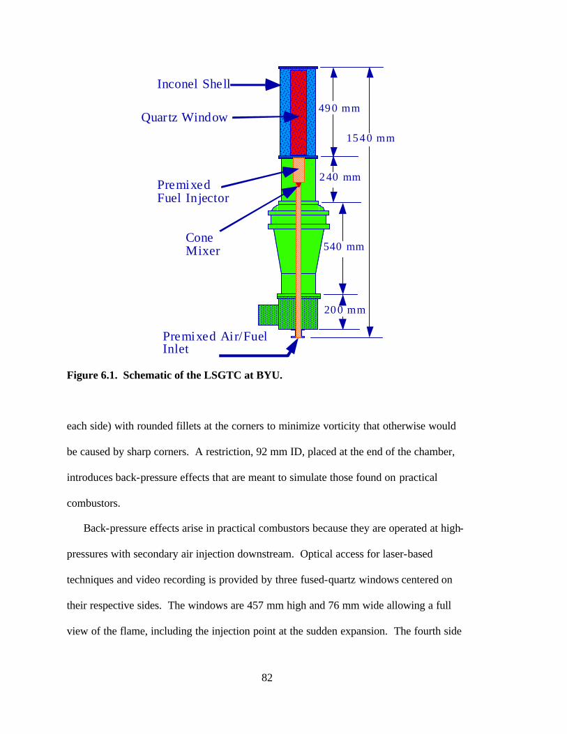
82
1540 mm
490 mm
240 mm
540 mm
200 mm
Quartz Window
Premixed Air/Fuel Inlet
PremixedFuel Injector
Inconel Shell
Cone Mixer
Figure 6.1. Schematic of the LSGTC at BYU. each side) with rounded fillets at the corners to minimize vorticity that otherwise would
be caused by sharp corners. A restriction, 92 mm ID, placed at the end of the chamber,
introduces back-pressure effects that are meant to simulate those found on practical
combustors.
Back-pressure effects arise in practical combustors because they are operated at high-
pressures with secondary air injection downstream. Optical access for laser-based
techniques and video recording is provided by three fused-quartz windows centered on
their respective sides. The windows are 457 mm high and 76 mm wide allowing a full
view of the flame, including the injection point at the sudden expansion. The fourth side
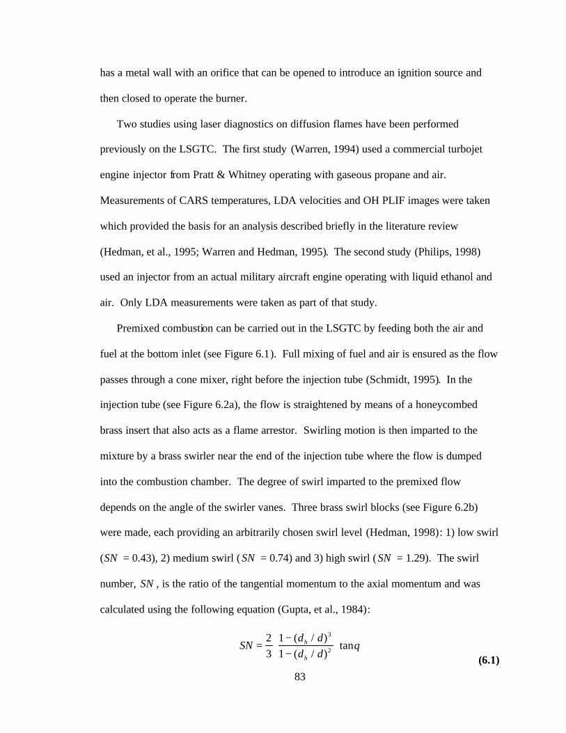
83
has a metal wall with an orifice that can be opened to introduce an ignition source and
then closed to operate the burner.
Two studies using laser diagnostics on diffusion flames have been performed
previously on the LSGTC. The first study (Warren, 1994) used a commercial turbojet
engine injector from Pratt & Whitney operating with gaseous propane and air.
Measurements of CARS temperatures, LDA velocities and OH PLIF images were taken
which provided the basis for an analysis described briefly in the literature review
(Hedman, et al., 1995; Warren and Hedman, 1995). The second study (Philips, 1998)
used an injector from an actual military aircraft engine operating with liquid ethanol and
air. Only LDA measurements were taken as part of that study.
Premixed combustion can be carried out in the LSGTC by feeding both the air and
fuel at the bottom inlet (see Figure 6.1). Full mixing of fuel and air is ensured as the flow
passes through a cone mixer, right before the injection tube (Schmidt, 1995). In the
injection tube (see Figure 6.2a), the flow is straightened by means of a honeycombed
brass insert that also acts as a flame arrestor. Swirling motion is then imparted to the
mixture by a brass swirler near the end of the injection tube where the flow is dumped
into the combustion chamber. The degree of swirl imparted to the premixed flow
depends on the angle of the swirler vanes. Three brass swirl blocks (see Figure 6.2b)
were made, each providing an arbitrarily chosen swirl level (Hedman, 1998): 1) low swirl
(SN = 0.43), 2) medium swirl (SN = 0.74) and 3) high swirl (SN = 1.29). The swirl
number, SN , is the ratio of the tangential momentum to the axial momentum and was
calculated using the following equation (Gupta, et al., 1984):
SN
d dd d
h
h
=−−
23
11
3
2
( / )( / )
tanθ (6.1)
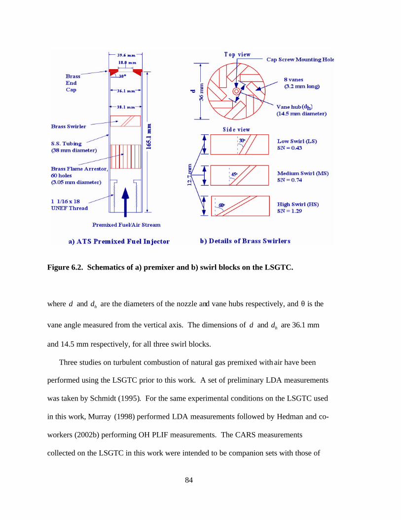
84
Figure 6.2. Schematics of a) premixer and b) swirl blocks on the LSGTC. where d and dh are the diameters of the nozzle and vane hubs respectively, and θ is the
vane angle measured from the vertical axis. The dimensions of d and dh are 36.1 mm
and 14.5 mm respectively, for all three swirl blocks.
Three studies on turbulent combustion of natural gas premixed with air have been
performed using the LSGTC prior to this work. A set of preliminary LDA measurements
was taken by Schmidt (1995). For the same experimental conditions on the LSGTC used
in this work, Murray (1998) performed LDA measurements followed by Hedman and co-
workers (2002b) performing OH PLIF measurements. The CARS measurements
collected on the LSGTC in this work were intended to be companion sets with those of
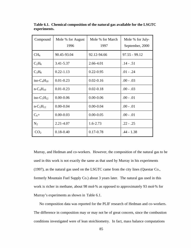
85
Table 6.1. Chemical composition of the natural gas available for the LSGTC experiments.
Compound Mole % for August
1996
Mole % for March
1997
Mole % for July-
September, 2000
CH4 90.45-93.04 92.12-94.66 97.55 - 99.12
C2H6 3.41-5.37 2.66-4.01 .14 - .51
C3H8 0.22-1.13 0.22-0.95 .01 - .24
iso-C4H10 0.01-0.23 0.02-0.16 .00 - .03
n-C4H10 0.01-0.23 0.02-0.18 .00 - .03
iso-C5H12 0.00-0.06 0.00-0.06 .00 - .01
n-C5H12 0.00-0.04 0.00-0.04 .00 - .01
C6+ 0.00-0.03 0.00-0.05 .00 - .01
N2 2.21-4.07 1.6-2.73 .22 - .25
CO2 0.18-0.40 0.17-0.78 .44 - 1.38
Murray, and Hedman and co-workers. However, the composition of the natural gas to be
used in this work is not exactly the same as that used by Murray in his experiments
(1997), as the natural gas used on the LSGTC came from the city lines (Questar Co.,
formerly Mountain Fuel Supply Co.) about 3 years later. The natural gas used in this
work is richer in methane, about 98 mol-% as opposed to approximately 93 mol-% for
Murray’s experiments as shown in Table 6.1.
No composition data was reported for the PLIF research of Hedman and co-workers.
The difference in composition may or may not be of great concern, since the combustion
conditions investigated were of lean stoichiometry. In fact, mass balance computations
86
show that the mole fraction of N2 in the combustion cases of interest is between 0.73 and
0.74 for all cases, regardless of which natural gas composition is used. However, it is
recommended that any future work account for the variation in natural gas composition in
any joint analysis of the CARS, LDA, and PLIF data.
6.1 Combustion Conditions
As stated earlier, this research examines the turbulent combustion of natural gas
premixed with air at atmospheric pressure in the LSGTC. However, to completely
specify a combustion condition, the stoichiometry, the inlet swirl level and the air flow
rate must be specified. Four combustion conditions (see Table 6.2) were selected at the
beginning of the ATS experimental program (Hedman, 1998), based on applicability to
industrial conditions as well as on combustion stability and operational limitations of the
facilities. These same conditions are the ones investigated in this work since these are the
only conditions for which LDA data are available (Murray, 1998).
Fuel lean conditions were chosen because that is how most modern industrial gas
turbines operate in order to avoid the emission of unburned fuel and to minimize NOx
production. Two equivalence ratios (φ) were selected (see Table 6.2). These values were
determined based on the Lean Blow-Out (LBO) limit of the LSGTC (φ about 0.56). At
this equivalence ratio, no sustainable combustion is achieved regardless of the inlet swirl.
The lowest value of φ at which stable combustion is obtained is 0.65. An intermediate
lean stoichiometry of 0.80 was chosen as a second value to include the effects of
stoichiometry in this study.
Three swirl levels are available for use in the LSGTC. However, preliminary runs on
the LSGTC showed that the combustion for the selected lean stoichiometries was too
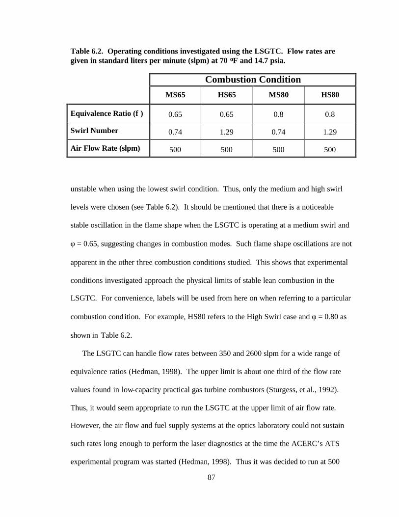
87
Table 6.2. Operating conditions investigated using the LSGTC. Flow rates are given in standard liters per minute (slpm) at 70 oF and 14.7 psia.
Combustion Condition MS65 HS65 MS80 HS80
Equivalence Ratio (φ ) 0.65 0.65 0.8 0.8
Swirl Number 0.74 1.29 0.74 1.29
Air Flow Rate (slpm) 500 500 500 500
unstable when using the lowest swirl condition. Thus, only the medium and high swirl
levels were chosen (see Table 6.2). It should be mentioned that there is a noticeable
stable oscillation in the flame shape when the LSGTC is operating at a medium swirl and
φ = 0.65, suggesting changes in combustion modes. Such flame shape oscillations are not
apparent in the other three combustion conditions studied. This shows that experimental
conditions investigated approach the physical limits of stable lean combustion in the
LSGTC. For convenience, labels will be used from here on when referring to a particular
combustion cond ition. For example, HS80 refers to the High Swirl case and φ = 0.80 as
shown in Table 6.2.
The LSGTC can handle flow rates between 350 and 2600 slpm for a wide range of
equivalence ratios (Hedman, 1998). The upper limit is about one third of the flow rate
values found in low-capacity practical gas turbine combustors (Sturgess, et al., 1992).
Thus, it would seem appropriate to run the LSGTC at the upper limit of air flow rate.
However, the air flow and fuel supply systems at the optics laboratory could not sustain
such rates long enough to perform the laser diagnostics at the time the ACERC’s ATS
experimental program was started (Hedman, 1998). Thus it was decided to run at 500
88
slpm based on a temperature of 70 oF and 14.7 psia of pressure. This is not thought to be
of major concern because experiments performed on the LSGTC by Hedman (1998)
showed that the dynamics of the flow (e.g., flame shape) did not change significantly
with total flow rates, as long as the stoichiometry was held constant. The flows were
measured and controlled by using the flow-metering system described by earlier
researchers (Murray, 1998; Pyper, 1994).
6.2 CARS Data Acquisition
The CARS data were collected on a vertical plane of the LSGTC’s combustion
chamber. This plane is parallel to and halfway between the two opposing quartz
windows for laser diagnostics in the LSGTC. In order to capture most details of the
flame, it is necessary to have a good spatial grid resolution as well as a sufficient number
of samples at each location for statistically reliable values of mean and standard
deviations. Results from preliminary CARS data sets obtained with the same spatial grid
reported by Murray (see Figure 6.3a) showed the need for more samples per location in a
finer grid in both the axial and radial directions. In this research, a spatial grid of 278
points (Figure 6.2b) that included the 126 LDA sampling locations used by Murray was
used. The exact number of locations sampled varied slightly for each combustion case
(see Appendix C). At each location, 1000 CARS samples were collected.
It should be noted that the combustion conditions that were studied involved the
reaction of the hydrocarbons in the natural gas (e.g., CH4) with the O2 in the air.
Reaction intermediates that promote the combustion, such as OH (e.g., Mallampalli, et
al., 1998), are generated during the reaction process culminating in the production H2O
and CO2. In this research, it was not possible to obtain CARS measurements of H2O,
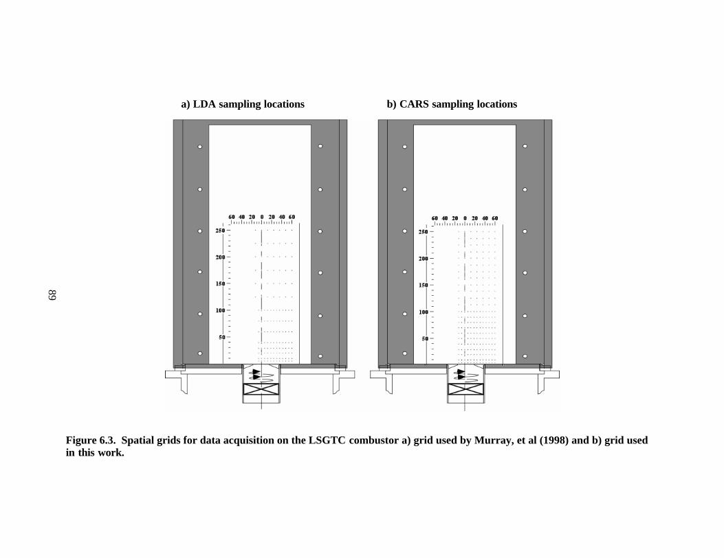
a) LDA sampling locations b) CARS sampling locations
Figure 6.3. Spatial grids for data acquisition on the LSGTC combustor a) grid used by Murray, et al (1998) and b) grid used in this work.
89

90
CH4 and the other hydrocarbons, and reaction intermediates because their respective
Raman Stokes frequencies are outside the wavelength range of the dual dye laser used.
91
7. RESULTS AND DISCUSSION
This chapter presents the results of the CARS temperature measurements, followed
by a discussion based on the following statistical values obtained from the instantaneous
temperature measurements: 1) averaged temperatures, 2) normalized standard deviations,
and 3) probability density functions of the instantaneous measurements. In addition, an
analysis is presented for one combustion case based on combined CARS, LDA (Hedman,
et al., 2002b) and PLIF OH (Hedman, et al., 2002a) measurements.
For brevity, only select plots of CARS temperature data are presented in this chapter;
however, additional plots are located in Appendix C. The complete set of instantaneous
temperature data at every sampling location of each combustion case are found in the CD
included in this dissertation.
7.1 CARS Temperature Contours
All contour plots to be presented were generated from the experimental CARS
temperature measurements using the software called “Transform” (version 3.4 from
Research Systems, Inc ). Each contour was based on an interpolated spatial mesh
produced by interpolating between the experimental data using the Kriging method—the
most accurate interpolation method according to the software documentation—with
Transform’s default parameters. The actual experimental data values were kept at their
original locations in the interpolated mesh, which ranged as follows: (1) in the radial
direction from -6 to 32 mm in increments of 0.5 mm; and (2) in the axial direction from 5
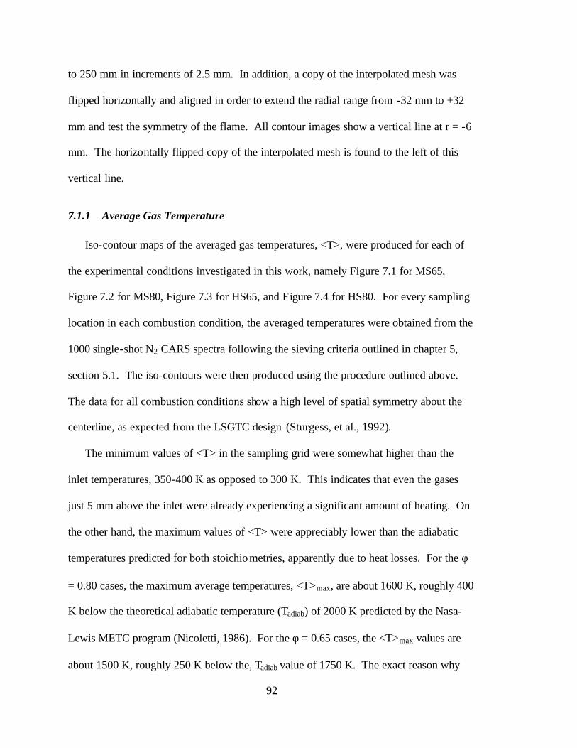
92
to 250 mm in increments of 2.5 mm. In addition, a copy of the interpolated mesh was
flipped horizontally and aligned in order to extend the radial range from -32 mm to +32
mm and test the symmetry of the flame. All contour images show a vertical line at r = -6
mm. The horizontally flipped copy of the interpolated mesh is found to the left of this
vertical line.
7.1.1 Average Gas Temperature
Iso-contour maps of the averaged gas temperatures, <T>, were produced for each of
the experimental conditions investigated in this work, namely Figure 7.1 for MS65,
Figure 7.2 for MS80, Figure 7.3 for HS65, and Figure 7.4 for HS80. For every sampling
location in each combustion condition, the averaged temperatures were obtained from the
1000 single-shot N2 CARS spectra following the sieving criteria outlined in chapter 5,
section 5.1. The iso-contours were then produced using the procedure outlined above.
The data for all combustion conditions show a high level of spatial symmetry about the
centerline, as expected from the LSGTC design (Sturgess, et al., 1992).
The minimum values of <T> in the sampling grid were somewhat higher than the
inlet temperatures, 350-400 K as opposed to 300 K. This indicates that even the gases
just 5 mm above the inlet were already experiencing a significant amount of heating. On
the other hand, the maximum values of <T> were appreciably lower than the adiabatic
temperatures predicted for both stoichiometries, apparently due to heat losses. For the φ
= 0.80 cases, the maximum average temperatures, <T>max, are about 1600 K, roughly 400
K below the theoretical adiabatic temperature (Tadiab) of 2000 K predicted by the Nasa-
Lewis METC program (Nicoletti, 1986). For the φ = 0.65 cases, the <T>max values are
about 1500 K, roughly 250 K below the, Tadiab value of 1750 K. The exact reason why
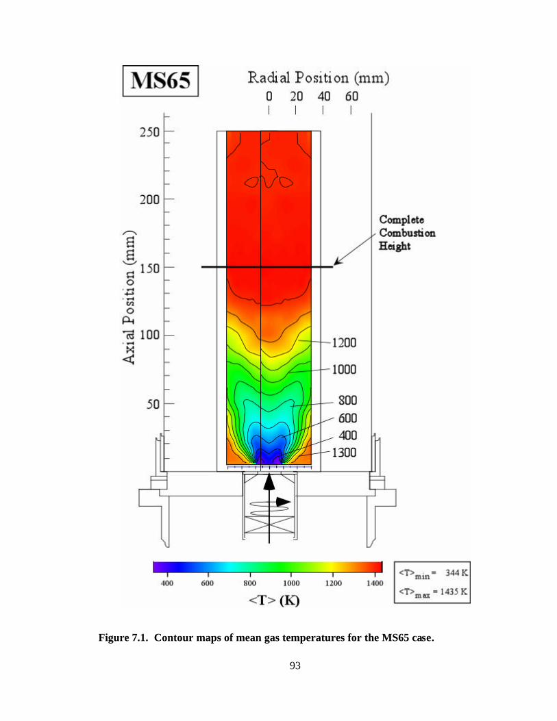
93
Figure 7.1. Contour maps of mean gas temperatures for the MS65 case.
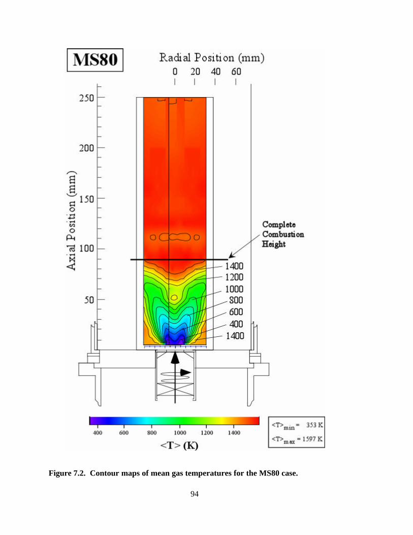
94
Figure 7.2. Contour maps of mean gas temperatures for the MS80 case.
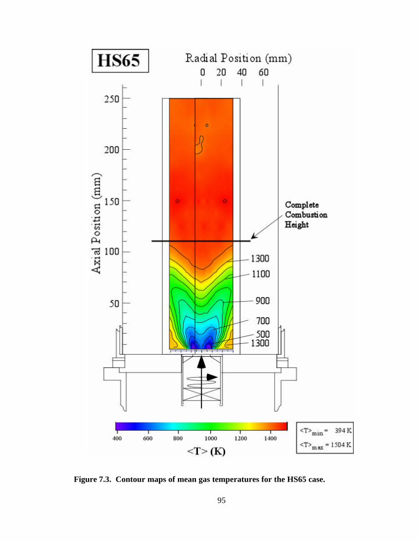
95
Figure 7.3. Contour maps of mean gas temperatures for the HS65 case.
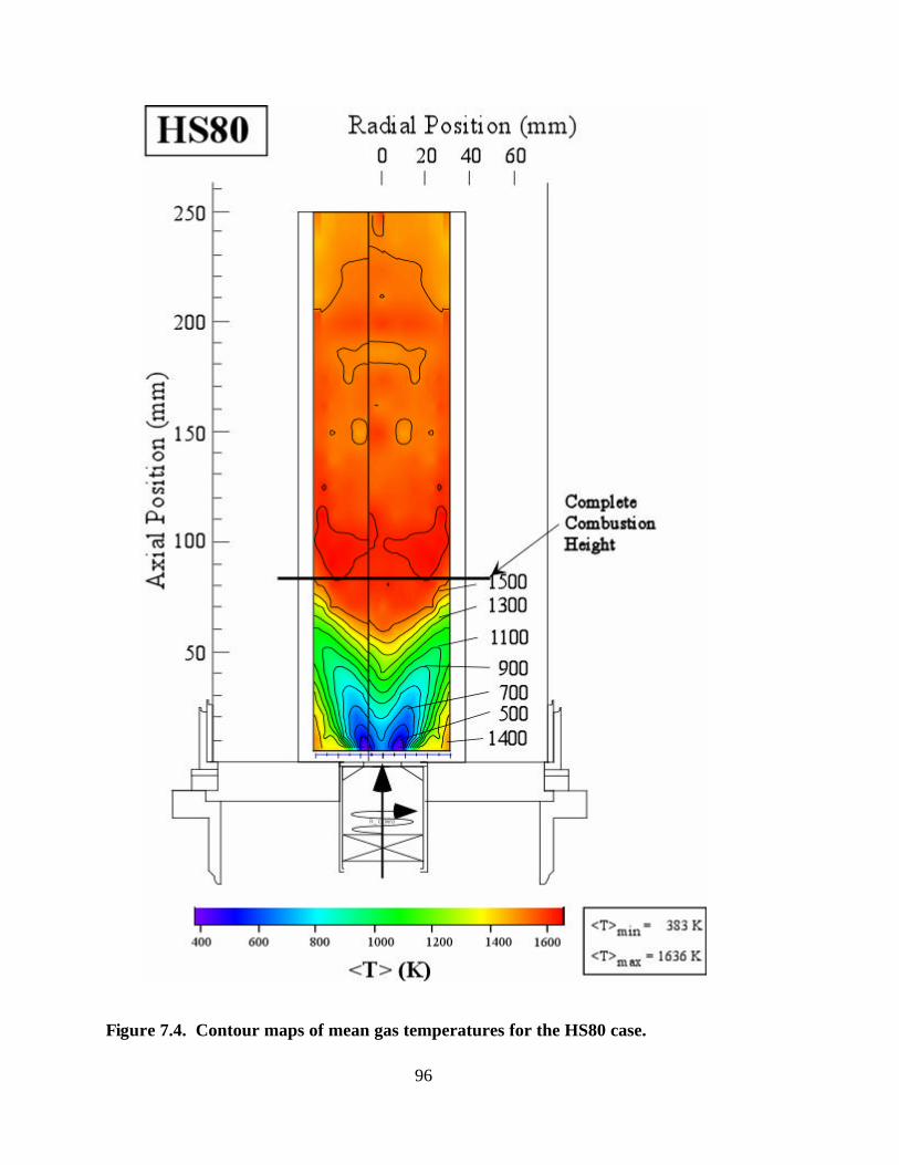
96
Figure 7.4. Contour maps of mean gas temperatures for the HS80 case.
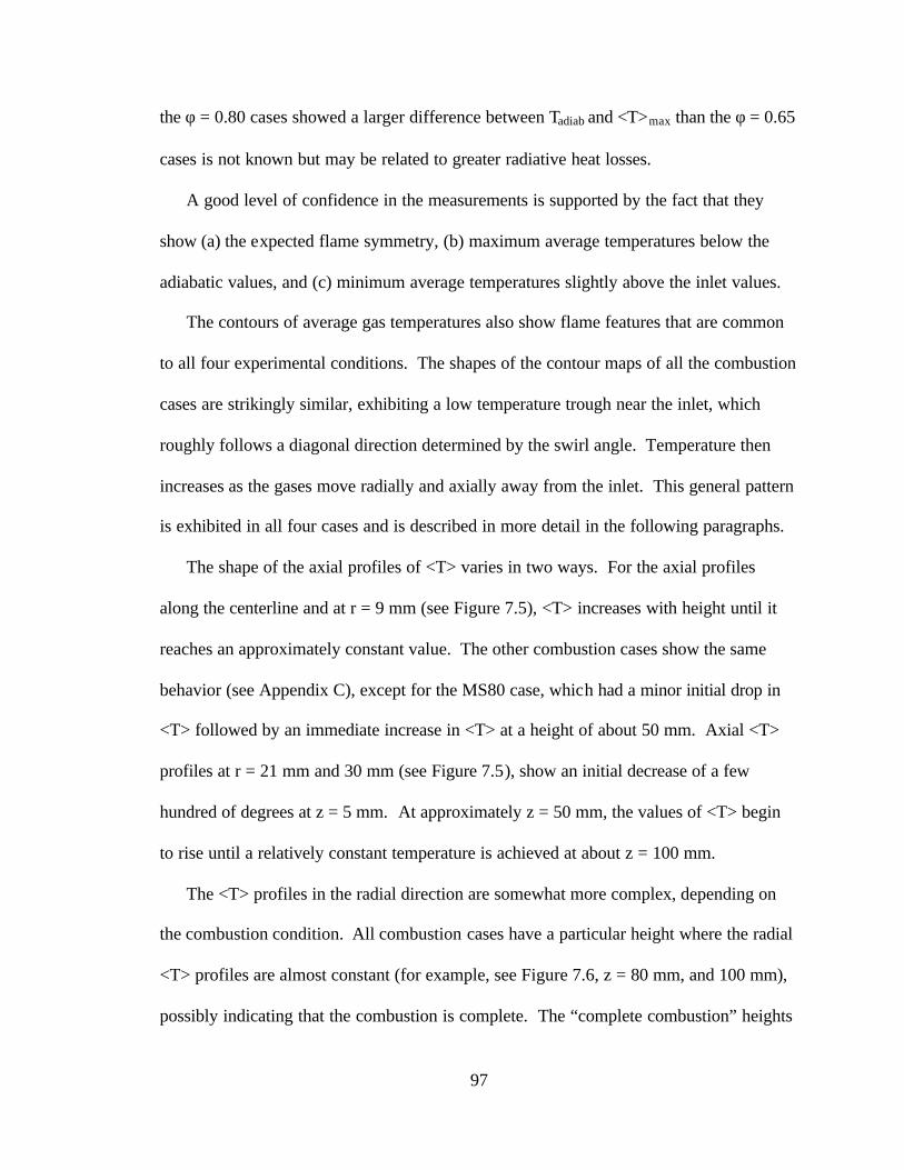
97
the φ = 0.80 cases showed a larger difference between Tadiab and <T>max than the φ = 0.65
cases is not known but may be related to greater radiative heat losses.
A good level of confidence in the measurements is supported by the fact that they
show (a) the expected flame symmetry, (b) maximum average temperatures below the
adiabatic values, and (c) minimum average temperatures slightly above the inlet values.
The contours of average gas temperatures also show flame features that are common
to all four experimental conditions. The shapes of the contour maps of all the combustion
cases are strikingly similar, exhibiting a low temperature trough near the inlet, which
roughly follows a diagonal direction determined by the swirl angle. Temperature then
increases as the gases move radially and axially away from the inlet. This general pattern
is exhibited in all four cases and is described in more detail in the following paragraphs.
The shape of the axial profiles of <T> varies in two ways. For the axial profiles
along the centerline and at r = 9 mm (see Figure 7.5), <T> increases with height until it
reaches an approximately constant value. The other combustion cases show the same
behavior (see Appendix C), except for the MS80 case, which had a minor initial drop in
<T> followed by an immediate increase in <T> at a height of about 50 mm. Axial <T>
profiles at r = 21 mm and 30 mm (see Figure 7.5), show an initial decrease of a few
hundred of degrees at z = 5 mm. At approximately z = 50 mm, the values of <T> begin
to rise until a relatively constant temperature is achieved at about z = 100 mm.
The <T> profiles in the radial direction are somewhat more complex, depending on
the combustion condition. All combustion cases have a particular height where the radial
<T> profiles are almost constant (for example, see Figure 7.6, z = 80 mm, and 100 mm),
possibly indicating that the combustion is complete. The “complete combustion” heights
98
Figure 7.5. Axial temperature profiles at selected radial positions for the HS80 case for each case are approximately as follows: (1) 150 mm for the MS65 case, (2) 90 mm for
the MS80 case, (3) 110 mm for the HS65 case, and (4) 90 mm for the HS80 case.
At the earliest axial position (z =5 mm) in Figure 7.6, a small peak in the <T> radial
profile is seen at the centerline (the peak is more apparent when the profiles are reflected
about the symmetry axis). A small trough in the shape of this temperature profile is
observed at r = 8 mm. The radial <T> values rise rapidly between r = 10 and 17 mm, and
then become nearly flat towards the wall. This shape of the radial <T> profile persists at
higher axial positions (see Figure 7.6), except that the radial location of the trough is
farther away from the centerline and the centerline peak becomes less noticeable.
For all combustion conditions, the magnitudes of the radial <T> gradients are
most severe near the inlet, specifically, at a height of 5 mm and a radial position of 9 mm.

99
Figure 7.6. Radial temperature profiles at selected heights for the HS80 case. <T> increases from about 400 K to about 1300 K occur over a radial distance of (1) 6
mm for the medium swirl cases, and (2) 9 mm for the high swirl cases. It should be noted
that the relative size of these radial distances is consistent with the fact that at a higher
swirl number the cold inlet mixture is injected at an angle that moves the flow closer to
the bottom plate. In this way, larger amounts of cold gas flow in the radial direction than
100
for lower swirl conditions; therefore, it takes longer to heat up the inlet gases at high
swirl conditions.
7.1.1.1 Flame Stability Observations
Variations in the flame stability of the combustion conditions were observed visually
during these experiments. Flame stability was determined subjectively in this work from
(a) the self-sustainability of the flame upon ignition with an external source, (b) the time
required to achieve steady state conditions, and (c) the degree of large-scale oscillations
in the flame shape. Less stable combustion conditions were difficult to light and tended
to self-extinguish unless exposed to the external ignition source for sufficient time. For
example, when lighting the MS65 condition, the external source needed to remain in the
flame for a period of 2-3 minutes before the flame could sustain itself. On the other
hand, when lighting the HS80 case, the flame sustained itself without the external
ignition source almost immediately after ignition.
Based on the flame stability observed during burner ignition, the combustion cases
were ranked according to decreasing degree of stability as follows: (1) HS80 (the most
stable case); (2) MS80; (3) HS65 (very similar to MS80); and (4) MS65 (the least stable).
Similar observations on flame stability were reported in previous studies for these cases
(Hedman, et al., 2002b; Murray, 1998).
There appears to be a direct relationship between the height of complete combustion
and the observations on flame stability just mentioned in the preceding paragraph: the
lower the height of completion, the higher the stability of the flame. The effect of φ on
flame stability is seen by the effect of φ on the height of completion (see Figure 7.1 and
Figure 7.2, or Figure 7.3 and Figure 7.4). It appears that the increased heat release due to
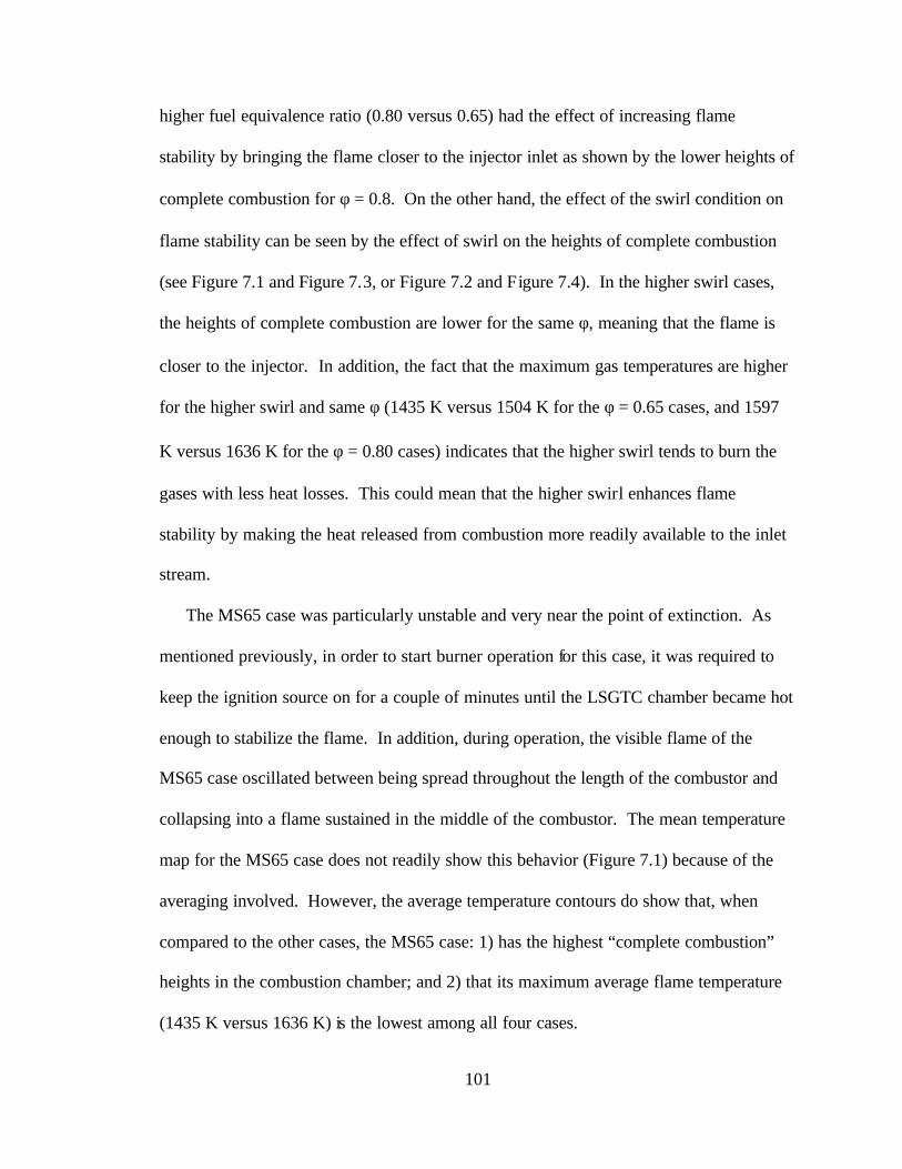
101
higher fuel equivalence ratio (0.80 versus 0.65) had the effect of increasing flame
stability by bringing the flame closer to the injector inlet as shown by the lower heights of
complete combustion for φ = 0.8. On the other hand, the effect of the swirl condition on
flame stability can be seen by the effect of swirl on the heights of complete combustion
(see Figure 7.1 and Figure 7.3, or Figure 7.2 and Figure 7.4). In the higher swirl cases,
the heights of complete combustion are lower for the same φ, meaning that the flame is
closer to the injector. In addition, the fact that the maximum gas temperatures are higher
for the higher swirl and same φ (1435 K versus 1504 K for the φ = 0.65 cases, and 1597
K versus 1636 K for the φ = 0.80 cases) indicates that the higher swirl tends to burn the
gases with less heat losses. This could mean that the higher swirl enhances flame
stability by making the heat released from combustion more readily available to the inlet
stream.
The MS65 case was particularly unstable and very near the point of extinction. As
mentioned previously, in order to start burner operation for this case, it was required to
keep the ignition source on for a couple of minutes until the LSGTC chamber became hot
enough to stabilize the flame. In addition, during operation, the visible flame of the
MS65 case oscillated between being spread throughout the length of the combustor and
collapsing into a flame sustained in the middle of the combustor. The mean temperature
map for the MS65 case does not readily show this behavior (Figure 7.1) because of the
averaging involved. However, the average temperature contours do show that, when
compared to the other cases, the MS65 case: 1) has the highest “complete combustion”
heights in the combustion chamber; and 2) that its maximum average flame temperature
(1435 K versus 1636 K) is the lowest among all four cases.
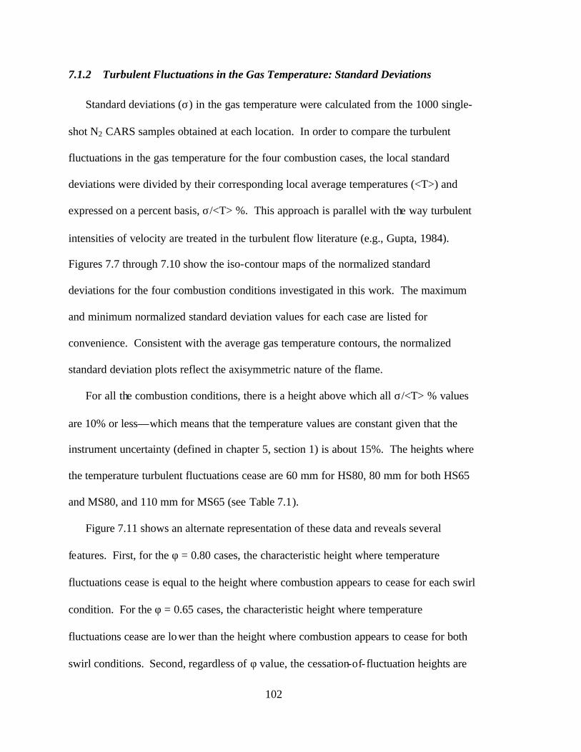
102
7.1.2 Turbulent Fluctuations in the Gas Temperature: Standard Deviations
Standard deviations (σ) in the gas temperature were calculated from the 1000 single-
shot N2 CARS samples obtained at each location. In order to compare the turbulent
fluctuations in the gas temperature for the four combustion cases, the local standard
deviations were divided by their corresponding local average temperatures (<T>) and
expressed on a percent basis, σ/<T> %. This approach is parallel with the way turbulent
intensities of velocity are treated in the turbulent flow literature (e.g., Gupta, 1984).
Figures 7.7 through 7.10 show the iso-contour maps of the normalized standard
deviations for the four combustion conditions investigated in this work. The maximum
and minimum normalized standard deviation values for each case are listed for
convenience. Consistent with the average gas temperature contours, the normalized
standard deviation plots reflect the axisymmetric nature of the flame.
For all the combustion conditions, there is a height above which all σ/<T> % values
are 10% or less—which means that the temperature values are constant given that the
instrument uncertainty (defined in chapter 5, section 1) is about 15%. The heights where
the temperature turbulent fluctuations cease are 60 mm for HS80, 80 mm for both HS65
and MS80, and 110 mm for MS65 (see Table 7.1).
Figure 7.11 shows an alternate representation of these data and reveals several
features. First, for the φ = 0.80 cases, the characteristic height where temperature
fluctuations cease is equal to the height where combustion appears to cease for each swirl
condition. For the φ = 0.65 cases, the characteristic height where temperature
fluctuations cease are lower than the height where combustion appears to cease for both
swirl conditions. Second, regardless of φ value, the cessation-of- fluctuation heights are
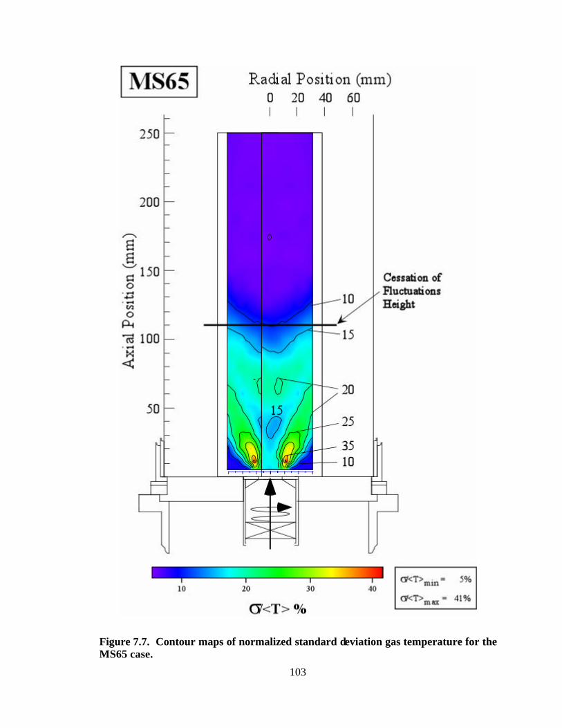
103
Figure 7.7. Contour maps of normalized standard deviation gas temperature for the MS65 case.
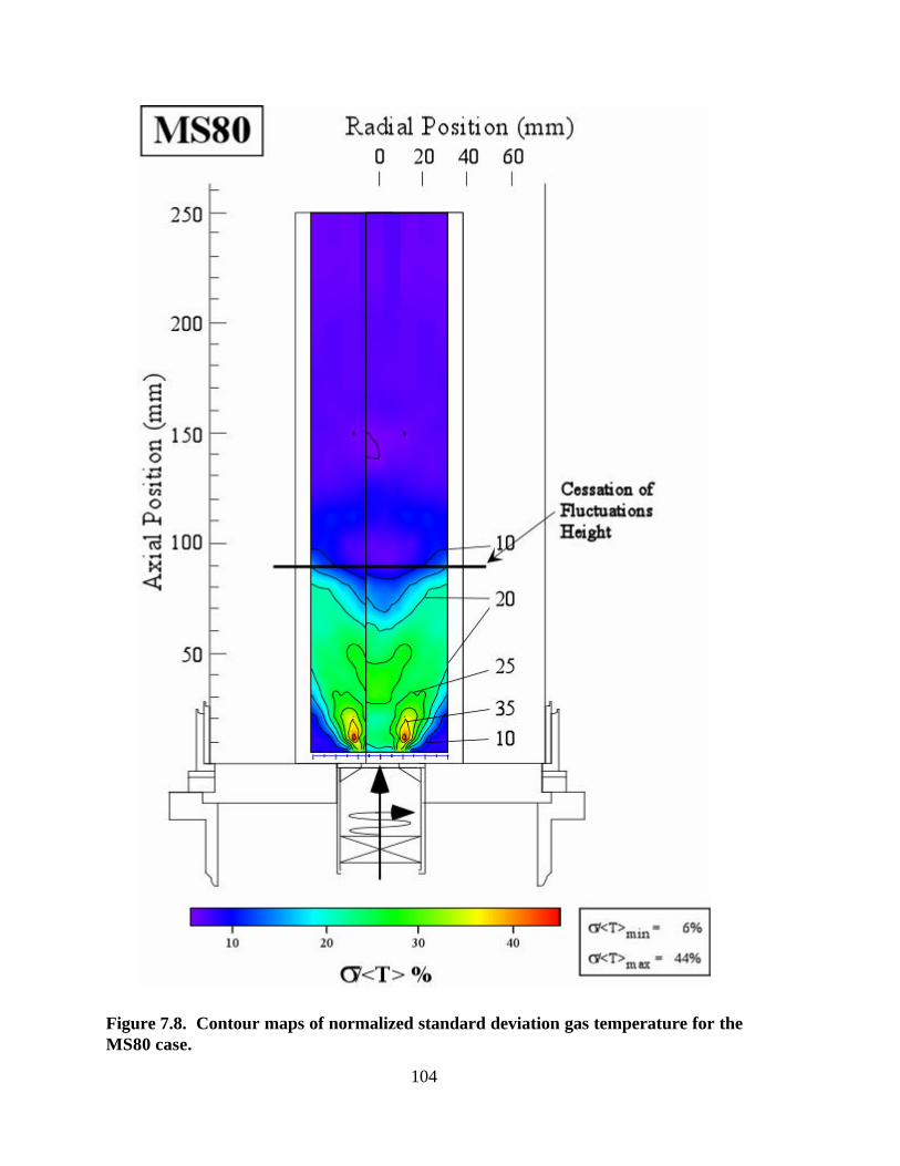
104
Figure 7.8. Contour maps of normalized standard deviation gas temperature for the MS80 case.
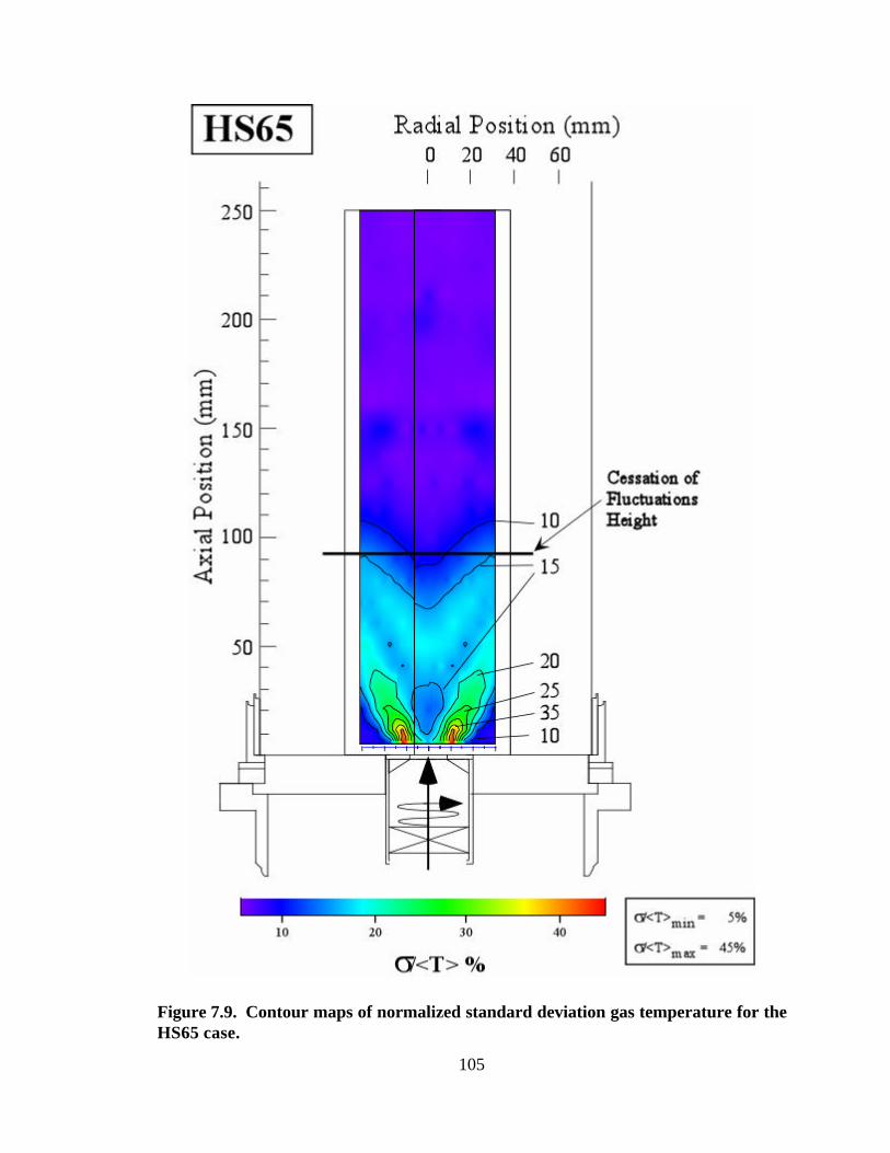
105
Figure 7.9. Contour maps of normalized standard deviation gas temperature for the HS65 case.
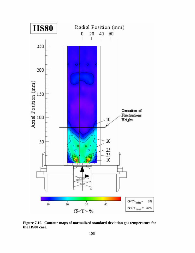
106
Figure 7.10. Contour maps of normalized standard deviation gas temperature for the HS80 case.
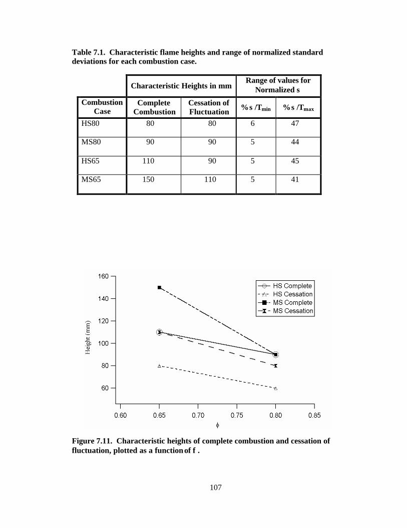
107
Table 7.1. Characteristic flame heights and range of normalized standard deviations for each combustion case.
Characteristic Heights in mm Range of values for
Normalized σ Combustion
Case Complete
Combustion Cessation of Fluctuation % σ/Tmin % σ/Tmax
HS80 80 80 6 47
MS80 90 90 5 44
HS65 110 90 5 45
MS65 150 110 5 41
Figure 7.11. Characteristic heights of complete combustion and cessation of fluctuation, plotted as a function of φ .

108
the lowest for the HS cases, while the heights of complete combustion are the highest for
the MS cases. Third, the cessation-of- fluctuation heights for the MS cases are only
slightly higher than the complete-combustion heights for the HS cases. These data show
that higher swirl tends to bring the reacting portion of the flame closer to the inlet, more
so than higher fuel content. It is well known that attached flames are generally more
stable than freestanding flames (Lewis and von Elbe, 1987). Based on visual
observations, profiles of <T>, and profiles of σ/<T>, it is therefore concluded that, for the
cases studied, the swirl level has a larger influence in bringing the flame closer to the
inlet than φ.
Figures 7.7 through 7.10 also show several common features for all cases. First, the
peak temperature fluctuations (σ/T % about 40%) are located in an area between 10 and
20 mm of height and between 15 and 20 mm of radius—just above the outer diameter of
the inlet. Second, all cases show temperature fluctuations (, i.e., σ/<T> % greater than
15%) throughout the combustor region below the heights of cessation of temperature
fluctuations with the exception of the bottom corners. Third, the temperature fluctuation
contours spread out diagonally upward from the inlet, decreasing in value but still
comparable to the temperature fluctuations along the centerline and below the height of
cessation of temperature fluctuations.
The temperature fluctuations data thus outlined in this section indicate that there is
mixing of cooler inlet gases with hot gases throughout the flame. However, the most
intense mixing of cold and hot gases exists very close to the inlet. It is possible that this
intense mixing near the inlet at least contributes to the ignition of the fresh inlet stream
and may even be the very source of ignition.
109
7.1.3 Gas Temperature Turbulent Fluctuations: Probability Density Functions
Probability density functions (PDFs) were obtained for every sampling location
throughout the combustor for each of the four combustion conditions. The PDFs were
obtained from histograms of the nearly 1000 instantaneous gas temperature
measurements at each location of interest in the spatial grid.
Four types of PDF distributions were found to exist in all combustion conditions (see
Figure 7.12): delta, beta, normal, and bimodal distributions. PDF plots were generated
for all radial positions away from the centerline at various axial positions: Figure 7.13
for z = 10 mm; Figure 7.14 for z = 50 mm; Figure 7.15 for z = 70 mm; and Figure 7.16
for z = 90 mm. Each figure consists of four columns of plots, one for each combustion
condition (i.e., MS65, MS80, HS65 and HS80). Appendix C contains similar figures for
additional heights. The PDF data give significant insights into the way hot and cold
gases are mixed at a specific location.
Each PDF has a “breadth” which is defined by the difference between the lowest- and
highest-temperature bins, i.e., the total width of the base of the PDF from the beginning
of the left wing to the end of the right one. Table 7.2 shows the relative occurrence for
each PDF expressed as the percent of the PDFs generated (z = 90 mm and below). In
general, beta distributions were the most frequent while the delta occurred the least.
The shape of each PDF distribution has a physical significance giving insights into
the nature of the temperature fluctuations at a given location. The PDF distributions can
be interpreted in the following ways:
1. A delta distribution implies a constant temperature because most of the
temperature measurements fall within one bin in the histogram. These
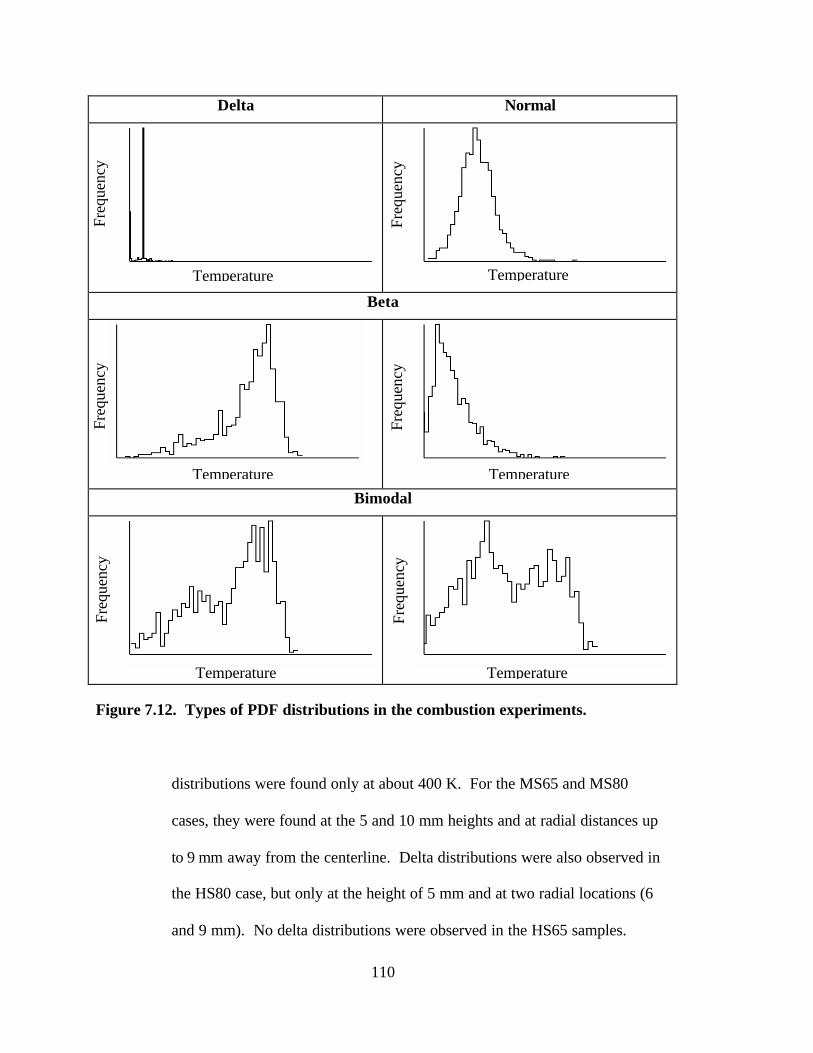
110
Delta Normal
Beta
Bimodal
Figure 7.12. Types of PDF distributions in the combustion experiments.
distributions were found only at about 400 K. For the MS65 and MS80
cases, they were found at the 5 and 10 mm heights and at radial distances up
to 9 mm away from the centerline. Delta distributions were also observed in
the HS80 case, but only at the height of 5 mm and at two radial locations (6
and 9 mm). No delta distributions were observed in the HS65 samples.
Temperature
Temperature
Temperature
Temperature
Temperature
Temperature
Freq
uenc
y
Freq
uenc
y
Freq
uenc
y
Freq
uenc
y
Freq
uenc
y
Freq
uenc
y
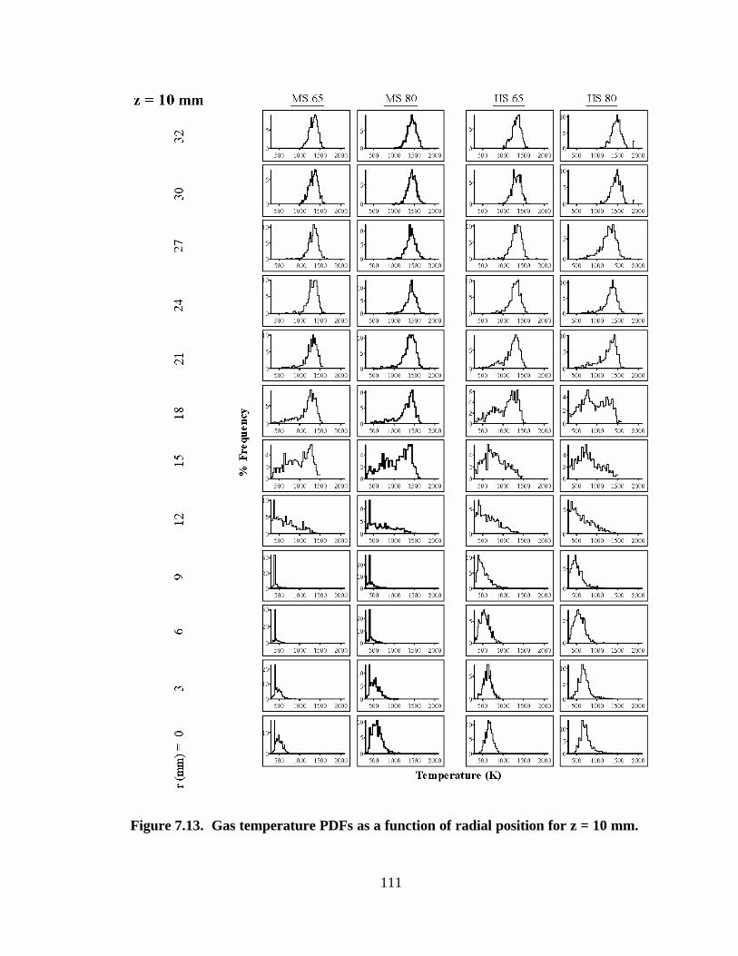
111
Figure 7.13. Gas temperature PDFs as a function of radial position for z = 10 mm.

112
Figure 7.14. Gas temperature PDFs as a function of radial position for z = 50 mm.

113
Figure 7.15. Gas temperature PDFs as a function of radial position for z = 70 mm.
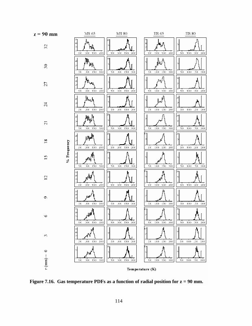
114
Figure 7.16. Gas temperature PDFs as a function of radial position for z = 90 mm.
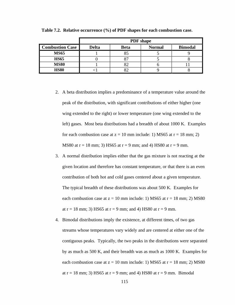
115
2. A beta distribution implies a predominance of a temperature value around the
peak of the distribution, with significant contributions of either higher (one
wing extended to the right) or lower temperature (one wing extended to the
left) gases. Most beta distributions had a breadth of about 1000 K. Examples
for each combustion case at z = 10 mm include: 1) MS65 at r = 18 mm; 2)
MS80 at r = 18 mm; 3) HS65 at r = 9 mm; and 4) HS80 at r = 9 mm.
3. A normal distribution implies either that the gas mixture is not reacting at the
given location and therefore has constant temperature, or that there is an even
contribution of both hot and cold gases centered about a given temperature.
The typical breadth of these distributions was about 500 K. Examples for
each combustion case at z = 10 mm include: 1) MS65 at r = 18 mm; 2) MS80
at r = 18 mm; 3) HS65 at r = 9 mm; and 4) HS80 at r = 9 mm.
4. Bimodal distributions imply the existence, at different times, of two gas
streams whose temperatures vary widely and are centered at either one of the
contiguous peaks. Typically, the two peaks in the distributions were separated
by as much as 500 K, and their breadth was as much as 1000 K. Examples for
each combustion case at z = 10 mm include: 1) MS65 at r = 18 mm; 2) MS80
at r = 18 mm; 3) HS65 at r = 9 mm; and 4) HS80 at r = 9 mm. Bimodal
Table 7.2. Relative occurrence (%) of PDF shapes for each combustion case.
PDF shape Combustion Case Delta Beta Normal Bimodal
MS65 1 85 5 9 HS65 0 87 5 8 MS80 1 82 6 11 HS80 <1 82 9 8

116
distributions would be expected in a shear layer created by a mixing interface
of fresh, unreacted inlet gases with fully reacted gases. This interaction would
result in eddies of hot and cold gases existing at different times at the same
location. It must also be mentioned that there were a few distributions as wide
as the bimodal distributions but with no definite peaks. It is believed that
these are special cases of a bimodal distribution where there is a more or less
continuous distribution of the gas temperatures.
Additional insights regarding the flame behavior were obtained by examining the
spatial variation in the shape of the PDFs for all the combustion conditions. First, the
maximum and mean temperatures of the PDFs for the φ = 0.80 cases were generally
higher than for the φ = 0.65 cases. This makes sense because more heat is released by the
combustion of more fuel at the higher equivalence ratio, which also agrees with the trend
in the adiabatic flame temperature.
Second, although the shapes of the PDFs varied both axially and radially for all cases,
it is interesting to examine the general location where similar trends in the PDF shapes
were observed:
1. For heights below 40 mm, (e.g., z = 10 mm in Figure 7.13), the shapes of the
PDFs for the MS65 and MS80 were essentially the same for the same radial
position, just shifted towards higher temperatures for the MS80 case. A
similar situation was also observed between the HS65 and HS80 cases.
However, the PDF shapes were significantly different for cases of different
swirl number and same φ. This seems to indicate that near the inlet, the

117
nature of the temperature fluctuations (and thus the cold/hot gas mixing) is
predominantly determined by the swirl level.
2. Close to the centerline and at heights of 40, 50, and 60 mm, the variation of
the shape of the PDFs was also a function of the radial position (e.g., z = 50
mm, see Figure 7.14). The observed shapes differed noticeably from case to
case suggesting that in this region the combined effects of both swirl and
equivalence ratios have significant impact.
3. At heights between 40 and 60 mm, the shapes of the PDFs were very similar
between combustion cases of the same equivalence ratio past a given radial
distance, which varied with height (e.g., r = 9 mm at z = 40, r = 18 mm at z =
50). This suggests that in this region the equivalence ratio controls the nature
of the PDFs more than the swirl level does.
4. At heights above 70 mm, the radial profiles of PDF shapes differed from case
to case as well (see Figures 7.13 and 7.14) suggesting that in this region the
combined effects of both swirl and equivalence ratio have significant impact.
Figure 7.17 shows the location of the bimodal distributions for the four combustion
cases. On the centerline, the bimodal distributions occur at the lowest height (50 mm) in
the 3 most stable cases, and at 60 mm for the least stable case (MS65). The bimodal
distributions occur along a diagonal from the bottom of the burner and outward radially,
possibly following a mixing layer along the inlet stream. The lowest heights where
bimodal distributions are observed appear to be a function of the inlet swirl number. The
two most stable cases, HS65 and HS80, show bimodal distributions at a height of 5 mm,
whereas the bimodal distributions are not observed below 10 mm for the MS cases. The
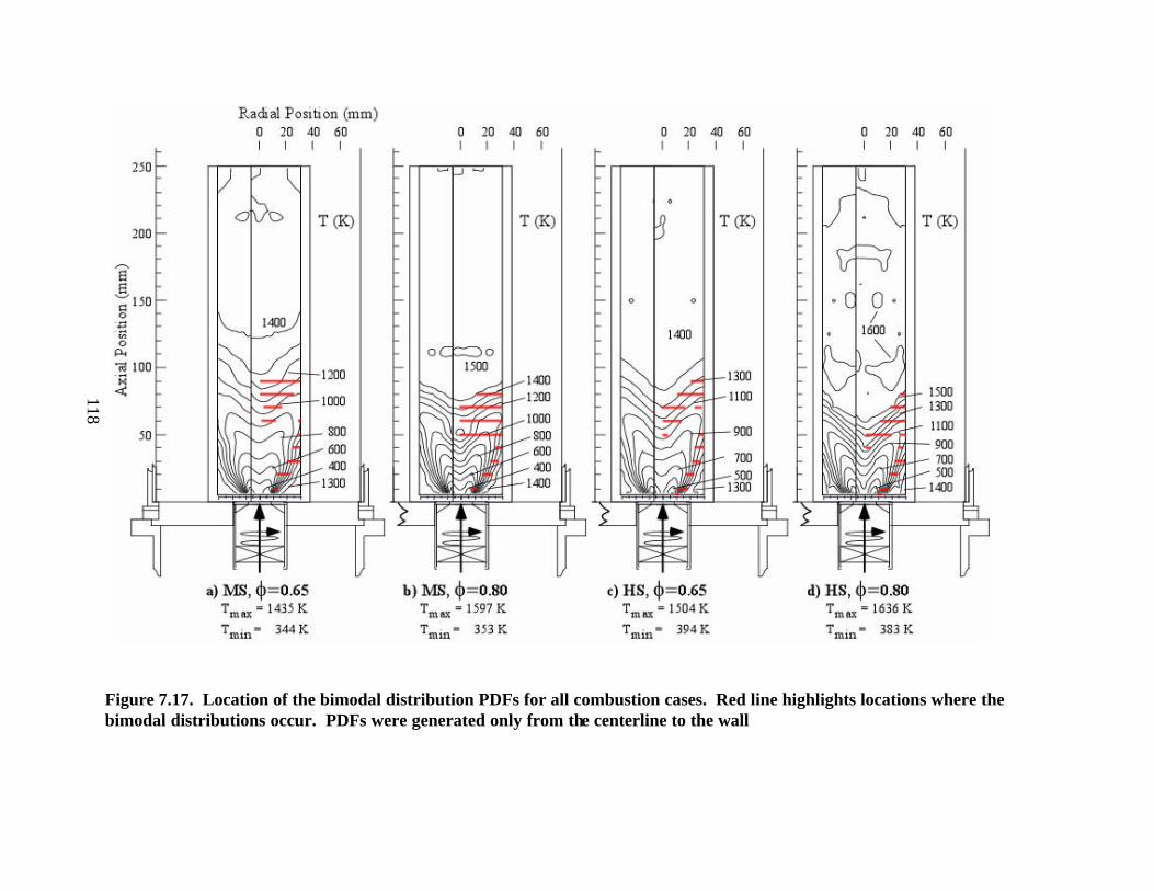
Figure 7.17. Location of the bimodal distribution PDFs for all combustion cases. Red line highlights locations where the bimodal distributions occur. PDFs were generated only from the centerline to the wall
118
119
highest height with bimodal distributions seems to be a function of φ, occurring at 90 mm
for the MS65 and HS65 cases, while occurring at 80 mm for the MS80 and HS80 cases.
It is interesting that the MS80 case is the only condition showing bimodal distributions
across the whole radius between z= 50 and 70 mm.
These observations indicate that bimodal distributions appear at lower heights in
more stable flames, both in the central recirculation zone and in the side recirculation
zone (recall Figure 2.5 in chapter 2, section 6). This is consistent with the idea that the
earlier (i.e., lower in height) the hot gases mix with the fresh stream, the more stable the
flame will be.
In conclusion, the study of the gas temperature PDFs has revealed certain patterns in
the complex nature of the mixing and reaction processes that take place in the LSGTC. It
is expected that this information will serve as the basis for future modeling studies in
order to explain the turbulent behavior of premixed combustion in systems similar to the
LSGTC. For a modeling theory to be successful, it should be able to identify both the
factors and mechanisms that determine what type of statistical variation will be found at a
given location in the combustor.
7.2 Comparison of CARS, PLIF and LDA data
The data collected in this work, together with Murray’s LDA data (1998) and
Hedman and co-worker’s PLIF OH data (2000a) present a great potential for fertile
research. LDA data show how the gas velocity varies throughout the combustor, giving
insights on how the inlet and reacted gases are transported into different areas of the
flame. PLIF OH data show qualitative concentrations of OH radical which is an
important intermediate during the combustion of natural gas. PLIF OH data also give
120
insights on whether the combustion has yet to start, has proceeded partially, or has been
completed at different locations throughout the flame.
In this section, an analysis is made by comparing CARS, LDA and PLIF OH data for
the most stable combustion case in this research, namely HS80, based solely on
experimental data. It must be remembered that these data were collected at different
occasions (about two years apart) and therefore the compositions of the natural gas used
in each experiment differed slightly. Ideally, it would be better to collect all three sets of
data simultaneously, or, if not possible, at least during the same time frame. A more
detailed analysis of the four data sets is beyond the scope of this dissertation.
The analysis to be presented below on the combined CARS, LDA and PLIF OH data
will rely on the LSGTC flow features described by Hedman, and co-workers (2002b).
Specifically, reference will be made to the flame vortex and the central and side
recirculation zones (CRZ and SRZ, respectively), as described in chapter 2, section 6 (see
Figure 2.5).
Figure 7.18 presents the false color image of the mean temperature data for the HS80
case found in Figure 7.4. A vector plot of the average axial and radial velocities from
Murray’s LDA data (Murray, 1998) is superimposed over the CARS gas temperature
data. The velocity vectors show:
1. The axial/radial velocity components of the vortex described by the strong
inlet flow moving diagonally upwards (tangential component not shown).
2. The CRZ (the flow inside the vortex center moving down towards the inlet).
3. The SRZ (the flow outside the vortex at the bottom corners moving towards
the centerline).

121
Figure 7.18. Averaged axial/radial velocity vector plot superimposed on the averaged CARS gas temperature map (left) and the average PLIF OH intensity image (right) for the HS80 case. The images are in the same scale and are aligned in height.
On the right side of Figure 7.18, a false color image of mean OH intensity for the
same combustion case is also included, as measured by Hedman, et al. (2002a). The
PLIF OH measurements are qualitative, with the red color representing the highest OH
76 mm
122
concentrations, the blue color the lowest OH concentrations, and the black color no
existence of OH. The velocity vectors are superimposed on the map of mean OH
intensity as well. The size of the vector arrows indicates the relative value of the
velocity—the larger the arrow, the larger the velocity.
The PLIF measurements did not yield quantitative values of OH concentration;
however, the intensity is nearly proportional to concentration, with the red color denoting
high concentration. The peak OH intensity is observed in the CRZ at a location centered
at about z = 60 mm. The OH structure shows “side arms” right next to the wall, which
seem to be curled down and pointing towards the center.
Another important feature of the OH map is the blue “halo”, i.e., the low
concentration region that surrounds the structure. These low concentration regions could
be interpreted in two different ways: either the OH is almost consumed, or it is beginning
to be formed. Determining what is actually happening at the top and bottom parts of the
halo in this regard warrants further research. It seems reasonable to assume that the top
halo is due to extinction of OH, while the bottom halo is due to the ignition started by the
mixing of the fresh inlet stream with the hot gases from both the central and the side
recirculation zones. In addition, the combined LDA and PLIF data appear to show that
the central recirculation zone is transporting the intermediate species such as the OH
radical down into the core of the flame vortex.
The idea that the bottom halo is an indicator of ignition seems to be supported by data
from the CARS, LDA and OH measurements. Figure 7.19 shows four instantaneous OH
images. The A-008 image is very similar to the averaged image (Figure 7.18), while
image B-126 shows an instance when the highest intensities occurred throughout the
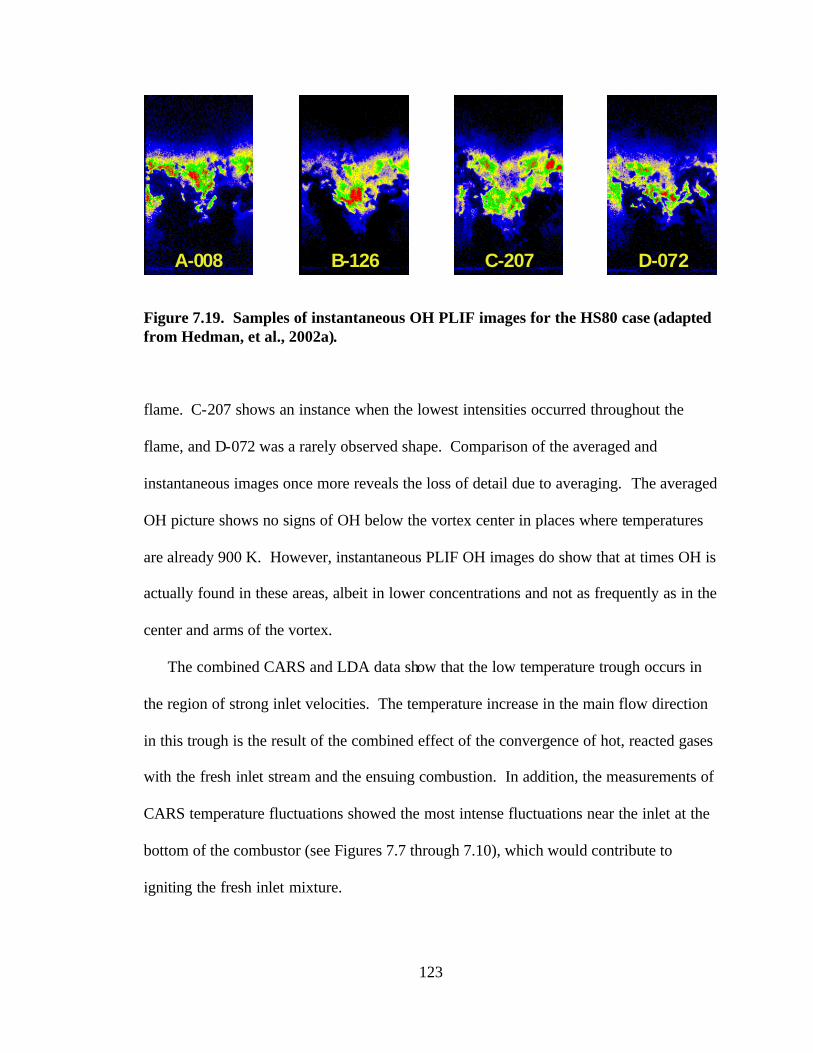
123
Figure 7.19. Samples of instantaneous OH PLIF images for the HS80 case (adapted from Hedman, et al., 2002a). flame. C-207 shows an instance when the lowest intensities occurred throughout the
flame, and D-072 was a rarely observed shape. Comparison of the averaged and
instantaneous images once more reveals the loss of detail due to averaging. The averaged
OH picture shows no signs of OH below the vortex center in places where temperatures
are already 900 K. However, instantaneous PLIF OH images do show that at times OH is
actually found in these areas, albeit in lower concentrations and not as frequently as in the
center and arms of the vortex.
The combined CARS and LDA data show that the low temperature trough occurs in
the region of strong inlet velocities. The temperature increase in the main flow direction
in this trough is the result of the combined effect of the convergence of hot, reacted gases
with the fresh inlet stream and the ensuing combustion. In addition, the measurements of
CARS temperature fluctuations showed the most intense fluctuations near the inlet at the
bottom of the combustor (see Figures 7.7 through 7.10), which would contribute to
igniting the fresh inlet mixture.
C-207B-126A-008 D-072

124
Another interesting observation based on Figure 7.18 is that the hot gases in the
central recirculation zone seem to cool down as they travel down the center of the vortex
while generating OH over a short distance. This may seem odd at first, but a plausible
explanation is proposed based on the following facts:
1. The temperature PDFs show a strong bimodal character in the vortex center in
the neighborhood of the 50 mm height near the centerline (e.g. PDFs A and B
in Figure 7.20, see Appendix C for more heights). This indicates that the
gases arriving at this region at different times have a wide bimodal variation
of temperature: one mode being centered at 900 K, with temperatures as low
as approximately 600 K, while the other mode being centered at 1500 K with
temperatures as high as approximately 1700 K.
2. The OH is found in the largest amounts in the vortex center at the 50 mm
height. This is shown by Figure 7.21 where several OH PDFs are shown at
various locations marked on the averaged OH image (same as Figure 7.18).
Note that the PDFs labeled B, C and D (at 50, 60 and 70 mm height on the
centerline, respectively) show the largest breadth of detector counts. Thus,
there is a wide variation with time at these locations in the OH content from
negligible to very high.
3. Although, on the average, the flow along the centerline goes downwards, there
is evidence that at times the flow does go upwards and from “side to side”
significantly (see discussion below).
The PDFs of the axial velocity component at three different radial positions at a
height of 80 mm are shown in Figure 7.22. The vertical red line indicates where the axial
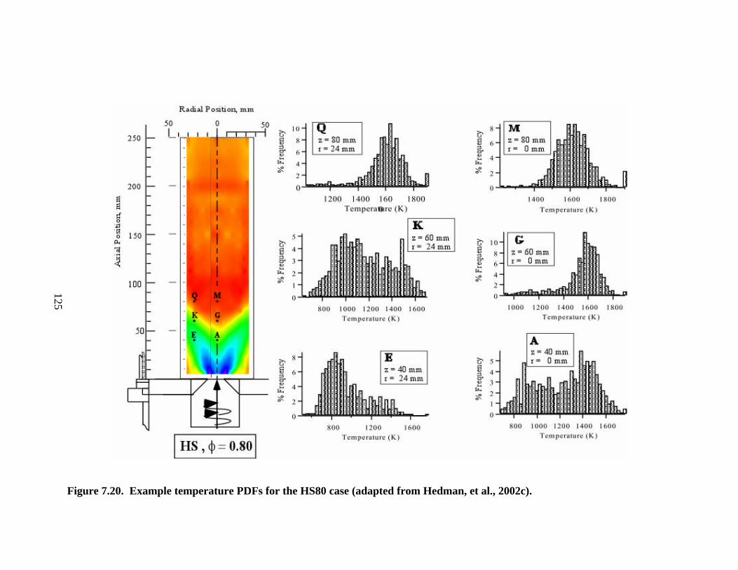
Figure 7.20. Example temperature PDFs for the HS80 case (adapted from Hedman, et al., 2002c).
125
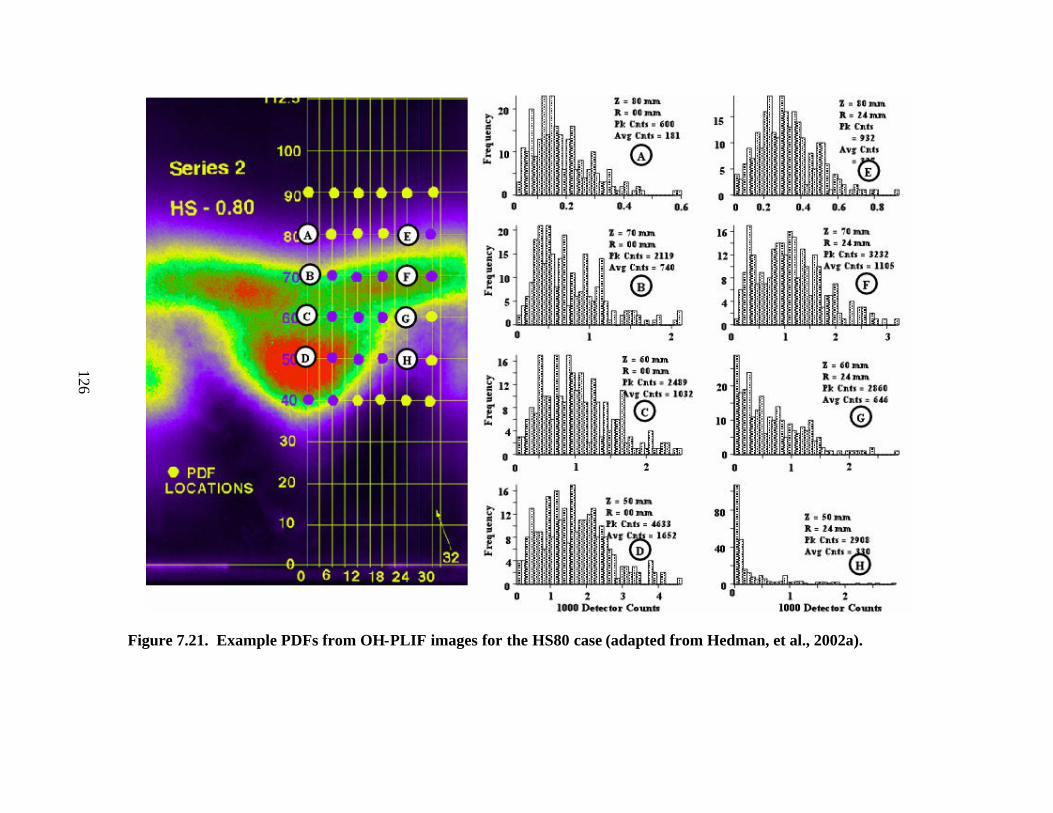
Figure 7.21. Example PDFs from OH-PLIF images for the HS80 case (adapted from Hedman, et al., 2002a).
126
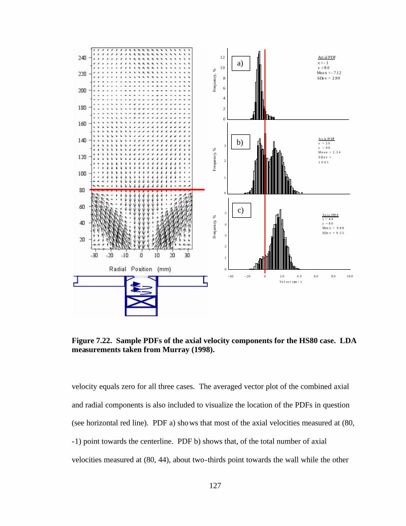
127
Figure 7.22. Sample PDFs of the axial velocity components for the HS80 case. LDA measurements taken from Murray (1998). velocity equals zero for all three cases. The averaged vector plot of the combined axial
and radial components is also included to visualize the location of the PDFs in question
(see horizontal red line). PDF a) shows that most of the axial velocities measured at (80,
-1) point towards the centerline. PDF b) shows that, of the total number of axial
velocities measured at (80, 44), about two-thirds point towards the wall while the other
3
2
1
0
A x ia lP DFx = 2 6z = 8 0M e a n = 2 .3 4S D e v =1 0 .6 1
Freq
uenc
y,%
5
4
3
Axi a l PD Fx = 4 4z = 8 0Mea n = 9.8 8SDe v = 9 .5 5
2
1
0
10 08 06 04 02 00- 20-40
Ve l oc i t ym / s
Freq
uenc
y,%
12
10
8
6
4
2
0
Axi al PDFx = - 1z = 8 0Mea n = - 7.12SDe v = 2.99
Freq
uenc
y,%
Vmax 47 m/s Vmin -22 m/s
a)
b)
c)
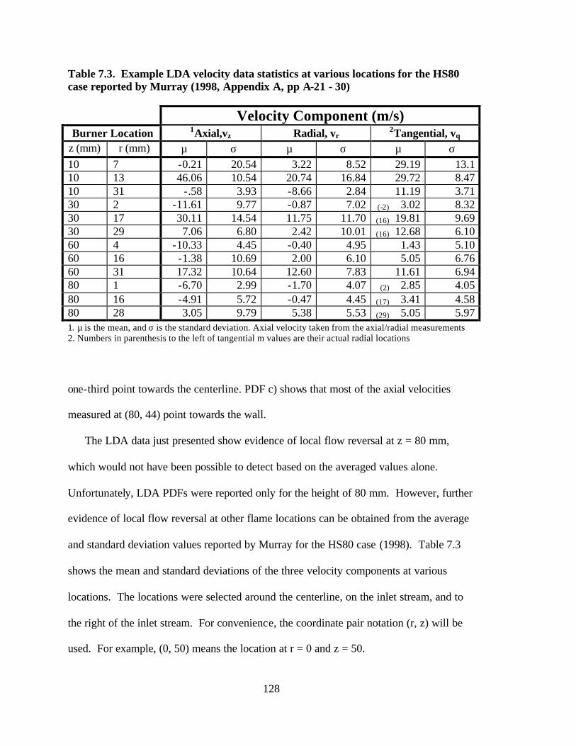
128
Table 7.3. Example LDA velocity data statistics at various locations for the HS80 case reported by Murray (1998, Appendix A, pp A-21 - 30)
Velocity Component (m/s) Burner Location 1Axial,vz Radial, vr 2Tangential, vθ
z (mm) r (mm) µ σ µ σ µ σ 10 7 -0.21 20.54 3.22 8.52 29.19 13.1 10 13 46.06 10.54 20.74 16.84 29.72 8.47 10 31 -.58 3.93 -8.66 2.84 11.19 3.71 30 2 -11.61 9.77 -0.87 7.02 (-2) 3.02 8.32 30 17 30.11 14.54 11.75 11.70 (16) 19.81 9.69 30 29 7.06 6.80 2.42 10.01 (16) 12.68 6.10 60 4 -10.33 4.45 -0.40 4.95 1.43 5.10 60 16 -1.38 10.69 2.00 6.10 5.05 6.76 60 31 17.32 10.64 12.60 7.83 11.61 6.94 80 1 -6.70 2.99 -1.70 4.07 (2) 2.85 4.05 80 16 -4.91 5.72 -0.47 4.45 (17) 3.41 4.58 80 28 3.05 9.79 5.38 5.53 (29) 5.05 5.97 1. µ is the mean, and σ is the standard deviation. Axial velocity taken from the axial/radial measurements 2. Numbers in parenthesis to the left of tangential m values are their actual radial locations one-third point towards the centerline. PDF c) shows that most of the axial velocities
measured at (80, 44) point towards the wall.
The LDA data just presented show evidence of local flow reversal at z = 80 mm,
which would not have been possible to detect based on the averaged values alone.
Unfortunately, LDA PDFs were reported only for the height of 80 mm. However, further
evidence of local flow reversal at other flame locations can be obtained from the average
and standard deviation values reported by Murray for the HS80 case (1998). Table 7.3
shows the mean and standard deviations of the three velocity components at various
locations. The locations were selected around the centerline, on the inlet stream, and to
the right of the inlet stream. For convenience, the coordinate pair notation (r, z) will be
used. For example, (0, 50) means the location at r = 0 and z = 50.

129
The data along the inlet stream (e.g., (13,10) and (29, 30)) have standard deviations
that are only a fraction of the size of their respective average values (e.g., 2/3 and 1/5).
This means that the averaged velocities along the inlet stream are a fair representation of
the direction of the flow. At either side of the inlet stream, however, the standard
deviations are equal to or greater than their corresponding average value. In these cases,
the average velocities do not represent the general direction of the flow since there is not
really one direction for the flow.
In fact, assuming that ± 2*σ represents the range of values of the measured velocities,
it can be concluded that the averaged velocities are hiding a large variation in the
direction of the flow. For example, at (10, 7), the axial velocities are –0.21 ± 20.54 m/s.
Thus, the axial velocity varied between +41 m/s (going upward) and – 41 m/s (going
downwards). In the case of the radial velocity at (10, 7) the component is +3.22 ± 8.52
m/s, thus the radial velocity varied between + 20 m/s (going towards the wall) and – 16
m/s (going towards the centerline). The velocity fluctuations in the tangential
components also show large variations.
Thus, all the velocity components outside the inlet stream and below the complete
combustion height flip their direction from time to time, as if there is a local reversal of
the flow. Using the ± 2*σ criterion, the data show that local flow reversal also exists in
the inlet stream, although not as noticeably as on its sides because here the σ values are
less than their corresponding averages. The flow reversals in all the velocity components
are a very strong indication of the existence of eddies in this region. Note that similar
situations were found in all the LDA data throughout the flame.

130
The facts just listed above may indicate that the gases present at the locations in and
around the vortex center have different extents of reaction at different times—sometimes
closer to ignition, and at other times almost fully reacted. This would explain why the
gas temperatures seem to cool off as the CRZ carries the flow down the centerline, as
gases closer to the inlet would be cooler than those at higher positions would. It is
proposed that this happens because the flow is carrying eddies into the center of the
vortex, sometimes from the top of the flame by the CRZ and at other times from the
strong inlet stream, possibly due to mixing with the SRZ. Moreover, it is possible that
the greater stability displayed by the HS80 case (compared to the other cases in this
work) is due to greater contributions of hot gases from the SRZ into the fresh inlet
stream.
7.3 Suggestions for Future Research
The preliminary analysis of combined LDA, PLIF and CARS for the HS80 case
presented in this work should be extended to the other three combustion conditions. The
combined analysis may make it possible to identify a potential zone of ignition sustained
by the mixing with the hot gases from both the central and side recirculation zones.
Again, the differences in the composition of the natural gas used throughout the LDA,
PLIF and CARS experiments should be factored in; otherwise, it would be preferable to
obtain new data simultaneously or at least in the same time frame.
Modeling studies, using advanced codes (e.g., Cannon, et al., 1999), should be
compared to the LDA, PLIF and CARS experiments in order to explain the turbulent
behavior of the premixed combustion in systems similar to the LSGTC. A successful
model should be able to identify both the factors and mechanisms that determine the type
131
and magnitude of the statistical variation throughout the combustor, matching as closely
as possible what experiments have shown. The model should also be able to explain the
roles that the central and side recirculation zones play in stabilizing the flame.
It would be interesting to pursue a chemical kinetic analysis using Lagrangian
pathlines (Warren and Hedman, 1995) generated from the mean values of LDA velocities
reported by Murray (1998) in conjunction with the temperature data collected in this
work. These pathlines represent the trajectory followed by a hypothetical packet of
premixed fuel and air. The Lagrangian path could be coupled with the CARS mean
temperature data to give the temperature history of the packet. The thermal history and
initial composition of the packet could then be used as input to 1-D chemical kinetic
models (e.g., the Premixed code by Kee, et al., 1992a). The chemical reactions can be
modeled using the CHEMKIN (Kee, et al., 1992b) subroutines with reduced kinetic
mechanisms for natural gas combustion (Mallampalli, et al., 1998) developed as part of
the ATS program at the Advanced Combustion Engineering Center of BYU. If further
work on the CARS instrument makes it possible to extract reliable values of O2 and CO2
concentrations, these experimental values could be compared with modeling predictions.
It is recognized that the turbulent effects would not be explicitly included in the
proposed Lagrangian analysis. This raises the following question: How closely can
turbulent premixed combustion be modeled using a temperature history from averaged
CARS and LDA data in a 1-D laminar premixed code? The answer either may help to
create new, simple models or may warrant the use of more sophisticated ones. The
outcome of this proposed analysis and the new knowledge derived from the CARS and

132
LDA joint analysis described above should be valuable information for both modelers
and designers.
133
8. CONCLUSIONS AND RECOMMEDATIONS
8.1 Conclusions
The CARS instrument development from this work resulted in the following unique
contributions:
1. An existing CARS instrument was modified to use a new single Stokes dual
dye laser that produces simultaneously CARS spectra of N2, CO, CO2, and O2.
These CARS spectra yield simultaneous values for the gas temperature,
derived from N2 measurements, and concentrations of CO, CO2, and O2. The
modified instrument requires less optical elements than dual Stokes CARS
systems and may therefore be advantageous to use in circumstances where
space availability is an issue.
2. New proportions of the pyromethene 650 and 597 dyes were used in order to
control the power and spectral characteristics of the Stokes dye laser used to
make the CARS instrument.
3. New software was developed to make it feasible to analyze the large
quantities of data acquired in this work in a reasonable amount of time. A
data management system was designed and implemented to automate the data
acquisition and reduction process. The data management system was coupled
with FMCARS, a CARS data reduction program developed in this work that
uses a CARS data reduction algorithm from Sandia National Laboratories.

134
4. Calibration studies in a tube furnace showed that the single Stokes CARS
instrument has good accuracy and acceptable precision for gas temperature
measurements. The average of the CARS measured values of gas
temperatures was within 5% of the thermocouple values of the tube furnace,
while the variability of the CARS measurements was within ±15% of the tube
furnace values.
5. Further calibration studies showed that the single Stokes instrument had
limited capabilities in measuring the concentrations of O2 and CO2 in the
concentration ranges of interest in this work.
a. Average O2 concentrations were about 15% less than the calibration
value, but the uncertainty on the measurements was at least 30%,
covering about two-thirds of the range of expected concentrations in
the combustion cases of interest.
b. Room temperature experiments showed that the instrument was simply
not reliable in obtaining CO2 concentrations.
It is possible that these limitations of the single Stokes instrument are due to
the approximations involved in the specific CARS reduction algorithm used in
this work.
6. The dual dye single Stokes CARS instrument was used to obtain
instantaneous gas temperature measurements for four combustion conditions
in a Laboratory Scale Gas Turbine combustor (LSGTC).
The following unique contributions were made while studying the gas temperature
CARS measurements obtained in the LSGTC:
135
1. Gas temperature measurements were obtained for four lean combustion
conditions of premixed natural gas and air. Two equivalence ratios, 0.65 and
0.80, were investigated at two different swirl levels.
2. Iso-contour plots of averaged and normalized standard deviations of gas
temperatures were produced based on the experimental data obtained in this work.
In addition, Probability Density Function (PDF) plots were also produced based
on the 1000 instantaneous measurements obtained at each sampling location.
3. It was found that flame stability in these combustion conditions increased with
increasing equivalence ratio and swirl level, which brought the flame vortex
closer to the inlet. The flame stability behavior observed in this work agrees with
prior research. The MS65 case, having the lowest equivalence ratio and inlet
swirl level, was the least stable case. On the other hand, the HS80 case, having
the highest equivalence ratio and inlet swirl level, was the most stable case.
4. Although the iso-contour plots of <T> and σ/<T> vary with combustion
conditions, the general shapes of the contours showed many similarities.
5. All cases exhibited a particular height where the radial temperature profiles are
almost constant and the normalized standard deviations are 5% or less, possibly
indicating that the combustion is complete. These data show that higher swirl
tends to bring the reacting portion of the flame closer to the inlet, more so than
higher fuel content.
6. Based on visual observations, profiles of <T>, and profiles of σ/<T>, it is
therefore concluded that, for the cases studied, the swirl level has a larger
influence in the stability of the flame than φ.
136
7. The normalized standard deviation plots and PDFs showed large variations in the
center of the vortex of each flame, supporting the assertion made by Hedman and
co-workers that the hot gases flowing down the centerline help stabilize the flame.
8. The normalized standard deviation plots also showed that the highest temperature
variations are found in a region just above the injector inlet. This feature lends
support to the idea that the side recirculation zone plays an important role
stabilizing the flame by helping to heat up and ignite the fresh inlet stream.
However, further research is recommended in order to assess to what extent the
turbulent mixing from the side recirculation contributes to the stability of the
flames.
9. Four types of PDF distributions were found to exist in all combustion conditions:
delta, beta, normal and bimodal distributions. Beta distributions were the most
prevalent in each combustion case. The locations of the bimodal distributions
seem to indicate that, for the more stable flames, the bimodal distributions occur
at the lowest heights in both the central recirculation zone and in the side
recirculation zone. This could mean that the earlier (i.e., lower in height) the hot
gases mix with the fresh stream, the more stable the flame will be. The study of
the gas temperature PDFs revealed the complex nature of the mixing and reaction
processes that take place in the LSGTC.
10. Additional insights regarding the flame behavior were obtained by examining the
spatial variation in the shape of the PDFs for all the combustion conditions. At
lower heights, near the bottom of the combustor, the swirl level seems to be the
dominant factor determining the nature of the turbulent fluctuations, whereas near
137
the wall and around z = 50 mm, the equivalence ratio appears to dominate. For
the rest of the flame, the combined effect of the equivalence ratio and swirl level
seems to determine the nature of the temperature fluctuations.
11. A preliminary analysis of combined LDA, PLIF, and CARS data for the HS80
case was presented. The combined analysis made it possible to identify a
potential zone of ignition, sustained by the mixing of inlet gases with the hot
gases from both the central and the side recirculation zones.
8.2 Recommendations
It is recommended that a comprehensive analyses comparing CARS, LDA and PLIF
OH data be performed for all combustion conditions in more detail. The differences in
the composition of the natural gas used throughout the LDA, PLIF and CARS
experiments should be accounted for; otherwise, it would be preferable to obtain new
data simultaneously or at least in the same time frame.
Future modeling studies should accompany the experiments in order to explain the
turbulent behavior of the premixed combustion in systems similar to the LSGTC. A
successful model should be able to identify both the factors and mechanisms that
determine the type and magnitude of the statistical variation throughout the combustor,
matching as closely as possible what experimentation has shown. The model should also
be able to explain the roles that the central and side recirculation zones play in stabilizing
the flame.
The following recommendations are made regarding the single Stokes dual dye
CARS instrument:

138
1. Investigate the possibility of using other dyes that would distribute the laser
power in the dye profile to minimize the power wasted in spectral regions of
no interest.
2. Compare the performance of the dual dye single Stokes CARS instrument
with the performance of the dual Stokes CARS instrument developed by
Boyack (1990).
3. Investigate whether the ability of the dual dye single Stokes CARS instrument
to measure O2 and CO2 concentrations can be improved by using a reduction
method that is more exact.
139
REFERENCES
Anand, M. S. and F. C. Gouldin, "Combustion Efficiency of a Premixed Continuous Flow Combustor," Journal of Engineering for Gas Turbines and Power, 107, 695-705 (1985).
Anderson, T. J., G. M. Dobbs and A. C. Eckbreth, "Mobile CARS Instrument for Combustion and Plasma Diagnostics," Applied Optics, 25, 4076-4085 (1986).
Armstrong, J. A., N. Bloembergen, J. Ducuing and P. S. Pershan, "Interaction between Light Waves in a Nonlinear Dielectric," Physical Review, 127, (6) 1918-1939 (1962).
Bedue, R., P. Gastebois, R. Bailly, M. Pealat and J. P. Taran, "CARS Measurements in a Simulated Turbomachine Combustor," Combustion and Flame, 57, 141-153 (1984).
Boyack, K. W., "A Study of Turbulent Nonpremixed Jet Flames of CO/N2 Using Coherent Anti-Stokes Raman Spectroscopy," Ph. D. Dissertation, Department of Chemical Engineering, Brigham Young University, Provo, UT (1990).
Buschmann, A., F. Dinkelacker, T. Schafer, M. Schafer and J. Wolfrum. Measurement of the Instantaneous Detailed Flame Structure in Turbulent Premixed Combustion. Twenty-Sixth Symposium (International) on Combustion, Univ. of California, Irvine, The Combustion Institute, 6, 437-445 (1996).
Cannon, S. M., B. S. Brewster and L. D. Smoot, "PDF Modeling of Lean Premixed Combustion Using In Situ Tabulated Chemistry," Combustion and Flame, 119, 233-252 (1999).
Cohen, H., C. F. C. Rogers and H. I. H. Saravanamuttoo. Gas Turbine Theory. Longman Group Limited, London (1996).
Druet, S. A. J. and J. P. E. Taran, "CARS Spectroscopy," Progress in Quantum Electrodynamics, 7, 1-72 (1981).
Eckbreth, A. C. Laser Diagnostics for Combustion Temperature and Species. Gordon and Breach Publishers (1996).
Ecob, D. J., M. B. Bouns and T. I. Mina, Using Natural Gas in Industrial Gas Turbines, Using Natural Gas in Engines, London, Mechanical Engineering Publications (1996).
140
Eesley, G. L. Coherent Raman Spectroscopy. Pergamon Press, New York (1981).
El Banhawy, Y., S. Sivasegaram and J. H. Whitelaw, "Premixed, Turbulent Combustion of a Sudden-Expansion Flow," Combustion and Flame, 50, 153-165 (1983).
Farrow, R., Personal Communication (1995).
Gupta, A. K., D. G. Lilley and N. Syred. Swirl Flows. Abacus Press, Malta (1984).
Hall, R. J. and L. R. Boedeker, "CARS Thermometry in Fuel-rich Combustion Zones," Applied Optics, 23, (9), 1340-1346 (1984).
Haslam, J. K., Personal Communication (1996).
Haslam, J. K. and P. O. Hedman. The Use of Two Pyromethene Dyes in a Single Stokes Dye Laser to Make CARS Temperature and Multiple Species (CO, CO2, O2, N2) Concentration Measurements. Fall Meeting of WSS/CI, 96F-086, Los Angeles, CA (1996).
Hay, N. E., Ed. Guide to New Natural Gas Utilization Technologies, The Fairmont Press, Inc. (1985).
Hedman, P. O., Personal Communication (1998).
Hedman, P. O., Personal Communication (2001).
Hedman, P. O., T. H. Fletcher, S. G. Graham, G. W. Timothy, D. V. Flores and J. K. Haslam. Observations of Flame Behavior in a Laboratory-Scale Pre-Mixed Natural Gas/Air Gas Turbine Combustor from PLIF Measurements of OH. ASME International Gas Turbine and Aeroengine Congress and Exposition, Amsterdam, Netherlands, International Gas Turbine Institute (2002a).
Hedman, P. O., R. L. Murray and T. H. Fletcher. Observations of Flame Behavior in a Laboratory-Scale Pre-mixed Natural Gas/Air Gas Turbine Combustor from LDA Velocity Measurements. ASME International Gas Turbine and Aeroengine Congress and Exposition, Amsterdam, The Netherlands (2002b).
Hedman, P. O., R. L. Murray and T. H. Fletcher. Observations of Flame Behavior in a Laboratory-Scale Pre-mixed Natural Gas/Air Gas Turbine Combustor from CARS Temperature Measurements. ASME International Gas Turbine and Aeroengine Congress and Exposition, Amsterdam, The Netherlands (2002c).
Hedman, P. O., L. D. Smoot, B. S. Brewster and T. H. Fletcher, "Combustion Modeling in Advanced Gas Turbine Systems," Final Report, Subcontract No. 93-01-SR014 (1998).
Hedman, P. O., G. J. Sturgess, D. L. Warren, L. P. Goss and D. T. Shouse, "Observations of Flame Behavior from a Practical Fuel Injector Using Gaseous Fuel in a

141
Technology Combustor," Journal of Engineering for Gas Turbines and Power, 117, 441-452 (1995).
Kataoka, H., S. Maeda and C. Hirose, "Effect of Laser Linewidth on the Coherent Anti-Stokes Raman Spectroscopy Spectral Profile," Applied Spectroscopy, 36, 508-512 (1982).
Kee, R. J., J. F. Grcar, M. D. Smooke and J. A. Miller, "A Fortran Program for Modeling Steady Laminar One-Dimensional Premixed Flames," SAND85-8240.UC-401 (1992a).
Kee, R. J., F. M. Rupley and J. A. Miller, "Chemkin-II: A Fortran Chemical Kinetics Package for the Analysis of Gas-Phase Chemical Kinetics," SAND89-8009B.UC706 (1992b).
Lefebvre, A. W. Gas Turbine Combustion. Hemisphere Publishing Corporation, New York (1983).
Lewis, B. and G. von Elbe, Combustion, flames and Explosions of Gases, Third Edition, Academic Press, San Diego, (1987).
Magre, P., P. Moreau, G. Collin, R. Borghi and M. Pealat, "Further Studies by CARS of Premixed Turbulent Combustion in a High Velocity Flow," Combustion and Flame, 71, 147-168 (1988).
Mallampalli, H. P., T. H. Fletcher and J. Y. Chen, "Evaluation of CH4/NOx Reduced Mechanisms Used for Modeling Lean Premixed Turbulent Combustion of Natural Gas," ASME Journal of Engineering for Gas Turbines and Power, 120, 703-712 (1998).
Melvin, A. Natural Gas: Basic Science and Technology. British Gas, London (1988).
Moya, F., S. A. J. Druet, M. Pealat and J. P. E. Taran, "Gas Spectroscopy and Temperature Measurement by Coherent Raman Anti-Stokes Scattering," Optics Communications, 13, 169-174 (1975).
Murray, R. L., "Laser Doppler Anemometry Measurements in a Turbulent, Premixed, Natural Gas/Air Combustor," M. S. Thesis, Department of Chemical Engineering, Brigham Young University, Provo (1998).
Nandula, S. P., R. W. Pritz, R. S. Barlow and G. J. Fiechtner. Rayleigh/Raman/LIF Measurements in a Turbulent Lean Premixed Combustor. 34th Aerospace Sciences Meeting and Exhibit, Reno, NV, American Institute of Aeronautics and Astronautics (1996).
Nguyen, Q. V., B. L. Edgar, R. W. Dibble and A. Gulati, "Experimental and Numerical Comparison of Extractive and In Situ Laser Measurements of Non-Equilibrium
142
Carbon Monoxide in Lean-Premixed Natural Gas Combustion," Combustion and Flame, 100, 395-406 (1995).
Nicoletti, P. A., "METCEC - User's Manual," Final Report for DOE Contract No. DE-AC21-85MC21353, Morgantown Energy Technology Center (April, 1986).
Palmer, R. E., "The CARSFT Computer Code for Calculating Coherent Anti-Stokes Raman Spectra: User and Programmer Information," Sandia Report SAND89-8206 (1989).
Pan, J. C. and D. R. Ballal. Chemistry and Turbulence Effects in Bluff-Body Stabilized Flames. 30th Aerospace Sciences Meeting & Exhibit, AIAA 92-0071, Reno, NV, American Institute of Aeronautics and Astronautics (1992).
Philips, C. G., "Laser Doppler Anemometry (LDA) Measurements in a Turbulent Ethanol Flame," M. S. Thesis, Department of Mechanical Engineering, Brigham Young University, Provo (1998).
Pyper, D. K., "The Study of Flame Stability Near Lean Blow Out in Non-Premixed Non-Swirl and Swirl Burners and the Design of a Research Combustor Facility," M. S. Thesis, Department of Mechanical Engineering, Brigham Young University, Provo (1994).
Regnier, P. R., F. Moya and J. P. E. Taran, "Gas Concentration by Coherent Raman Anti-Stokes Scattering," AIAA J., 12, 826-831 (1974).
Regnier, P. R. and J. P. Taran, "On the Possibility of Measuring Gas Concentrations by Stimulated Anti-Stokes Scattering," Applied Physics Letters, 23, 240-242 (1973).
Roberts, W. L., J. F. Driscoll, M. C. Drake and L. P. Goss, "Images of the Quenching of Flame by a Vortex-To Quantify Regimes of Turbulent Combustion," Combustion and Flame, 94, 58-69 (1993).
Rudd, M. J., "A New Theoretical Model for the Laser Dopplermeter," Journal of Physics E, 2, (55) (1969).
Schmidt, S. E., "Laser Doppler Anemometry (LDA) Measurements in a Turbulent Premixed Natural Gas Flame," M. S. Thesis, Department of Chemical Engineering, Brigham Young University, Provo (1995).
Schmidt, S. E. and P. O. Hedman, "CARS Temperature and LDA Velocity Measurements in a Turbulent Swirling, Premixed Propane/Air Fueled Model Gas Turbine Combustor," 95-GT-64 (1995).
Snelling, D. R., G. G. Smallwood and T. Parameswaran, "Effect of detector nonlinearity and image persistence on CARS derived temperatures," Applied Optics, 28, (15) 3233-3241 (1989).
143
Snelling, D. R., G. J. Smallwood, R. A. Sawchuk and T. Parameswaran, "Precision of Multiplex CARS Temperatures Using Both Single-Mode and Multimode Pump Lasers," Applied Optics, 26, 99-110 (1987).
Sturgess, G. J., D. G. Sloan, A. L. Lesmerises, S. P. Henneghan and D. R. Ballal, "Design and Development of a Research Combustor for Lean Blow-Out Studies," ASME Journal of Engineering for Gas Turbines and Power, 114, 13-19 (1992).
Switzer, G. L., L. P. Goss, W. M. Roquemore, R. P. Bradley, P. W. Schreiber and W. B. Roh, "Application of CARS to Simulated Practical Combustion Systems," Journal of Energy, 4, 209-215 (1982).
Teets, R. E., "Accurate Convolutions of Coherent Anti-Stokes Raman Spectra," Optics Letters, 9, 226-228 (1984).
Tolles, W. M. and A. B. Harvey, Introduction to Nonlinear Phenomena, Chemical Applications of Nonlinear Raman Spectroscopy. A. B. Harvey, Washington, D. C., Academic Press, (1981).
Tolles, W. M., J. W. Nibler, J. R. McDonald and A. B. Harvey, "A Review of the Theory and Application of Coherent Anti-Stokes Raman Spectroscopy (CARS)," Applied Spectroscopy, 31, (4) 253-271 (1977).
Warren, D. L., "Combustion Studies of a Swirled, Non-Premixed Flame Using Advanced Diagnostics," M. S. Thesis, Department of Mechanical Engineering, Brigham Young University, Provo (1994).
Warren, D. L. and P. O. Hedman, "Differential Mass and Energy Balances in the Flame Zone from a Practical Fuel Injector in a Technology Combustor," Transactions of the ASME, 95-GT112 (1995).
Whiting, E. E., "An Empirical Approximation to the Voigt Profile," Journal of Quantitative Spectroscopy and Radiative Transfer, 8, 1379-1384 (1968).
Yeh, Y. and H. Z. Cummins, "Localized Fluid Flow Measurements with an He-Ne Laser Spectrometer," Applied Physics Letters, 4, 176-178 (1964).
Yuratich, M. A., "Effects of Laser Linewidth on Coherent Anti-Stokes Raman Spectroscopy," Journal of Molecular Physics, 38, 625-655 (1979).
Zhu, J. Y., T. Tsuruda, W. A. Sowa and G. S. Samuelsen, "Coherent Anti-Stokes Raman Scattering (CARS) Thermometry in a Model Gas Turbine Can Combustor," Journal of Engineering for Gas Turbines and Power, 115, 515-521 (1993).

144