Embed Size (px)
Citation preview
'~".'.."
ANALYSIS OF GRILLAGES SUBJECTED TO COMBINED LOADS
by
Robert P. Kerfoot
A Dissertation
Presented to the Graduate Committee
of Lehigh University
in Candidacy for the Degree of
Doctor of Philosophy
mrrz ENmNEERtNGLABORATORY LIBRARY
in
Civil Engineering
Lehigh University
1972.

ACKNOWLEDGMENTS
The work reported in this thesis was performed as part of a
research project, Grillsges Under Normal and Axial Loads, conducted in
the Department of Civil Engineering at Fritz' Engineering Laboratory,
Lehigh University, Bethlehem, Pennsylvania. Dr. David A. VanHorn is
Chairman of the Department and Dr. Lynn S. Beedle is Director of the
Laboratory.
The author gratefully acknowledges the sponsorship of the
project by the Naval Ship Engineering Center of the Department of the
Navy. Messrs. Donald S. Wilson and Elias R. Ashey of NavSEC deserve
special mention becuase of the encouragement,guidance, and confidence
extended during the study.
The author is deeply indebted to Dr. Alexis Ostapenko,
director of the research program and Professor in Charge of the
dissertation. His encou!"agement, advice, counsel, and assistance are
deeply appreciated. The guidance of. the other members of the special
connnittee directing the author's doctoral program, Drs. David A.
VanHorn, Lynn S. Beedle, Fazil Erdogan, and Le-Wu Lu, is grc;ltefully
acknowledged.
Mr. Siamak Parsanejad merits special recognition and thanks
for his contribution in programming, evaluation of search techniques,
preparation of some of the figures, and in the time-consuming production
of a preliminary version of the thesis submitted as a research report
to.the sponsor.iii

.. '.-
The thesis was typed by Mrs. Jane Lenner and Miss Shirley
Matlock. Their cooperation and patience with the lengthy equations
in particular are appreciated. Most of the figures were drawn by
Mrs. Sharon Balogh whose careful efforts are appreciate4 .
"., iv

TAl3LE OF CONTENTS
Page, '
ABSTRACT
1. INTRODUCTION
1.1 The Ship Grillage1.2 Design Requirements1.3 Currently Available Methods of Analysis
:1
3
357
1.3.11.3.21. 3. ~ ,1.3"41.3.5
PIate and :Beam TheoryDiscrete Element MethodsTreatment as a :Beam GridOrthotropic Plate Theory ,Conclusions Concerning ExistingAnalytical Methods '
7789
11
1.4 Objective.s and Scope of this Investigation 11
ObjectivesScope
11,12
2. INELASTIC PLATE THEORY 15
2.1 Introduction 152.2 Assumptions and Limitations 162.3 Equilibrium Equations for a Plate Differential 18
Element2.4 The Generalized Stress...Strain Law 202.5 The Plate Differential Equations 282.6 Resume 31
3. INELASTIC :BE:AMTHEORY
3.1 Introduction3.2 Assumptions and Limitations3.3 Equilibrium of a Differential Element3.4 The Generalized Stress-Strain Law3.5 :Beam Displacements as Functions of Plate
Displacements'3.6 ResUme
4. LOADS AND BOUNDARY CONDITIONS
4.1 Introduction4.2 Loads Applied by Beams
4.2.1 Junction of Plate and a Single :Beam4.-2.2 Junction of Plate and, Two Beams
4.3 Force Boundary Conditions
'v
32'
32 33353846
47
49
494~
5q55
58
4.4 Displacement Boundary Conditions4;5 Mixed Boundary Conditions4.6 Resume
5. THE DISPIACEMENT FUNCTIONS
5.1 Introduction5.2 The Form of the 'Displacement Functions5.3 Characteristics Required of the Bending
Displacement Functions5.4 Functions Employed to Define the Bending
Displacement '5.5 Characteristics Requtred of In-Plane
Displacement Functions5.6 Functions Employed to Define In-Plane
Displacements5.7 Combination of the Product Functions5.8 Resume
6. PROPOSED METHOD OF SOLUTION
6.1 The Method of Collocation6.2 A Variant of the Method of Collocation
6.2.1 'The Search Method6.2.2 The Valley Point Problem6.2.3 A Cautionary Note Regarding Symmetry
. -: ... .; ..6.3 The Total Error Function for a Grillage6.4 ,Application of the Proposed Method
59'6262
64
6464
66
69
72
7578
.78
80
8081
818486
8790
6.4.16.4.2
6.4.3
The Computer ProgramSelection of Initial Values ofConstant CoefficientsPoints Selected to Define Errors
9092
93
6.5 Example Problem6.6 Resume
7. SUMMARY, CONCLUSIONS, AND RECOMMENDATIONS,
7.1 ,Sunnnary7.2 Conclusions7.3 Recommendations for Future Work
8. REFERENCES
9. NOTATION
10. FIGURESvi
96101
103
103106108
112
119
122

11. APPENDIXES ';
12. VITA
vii
Page
146
186

ABSTRACT
A method is presented for the large deflection analysis of
grillages subjected to combined normal and axial loads. The analysis
of the grillage is reduced to the analysis of the grillage plate
subjected to two simultaneously applied sets of loads; one set applied
by agencies external to the grillage and independent of the grillage
deformations. and the other set comprised of the distributed redundant
tractions and couples which act between the grillage plate and beams
and are functions of the deformations of the grillage. The method is
a displacement formulation in which a variant of the method of colloca
tion is employed to develop approximate solutions to the coupled non
linear differential equations which define the large displacement
inelastic behavior of plates and beam columns.
To develop the method a generalized stress-strain law is
first develo~ed for a differential element of a plate composed of an
elastic-perfectly-plasti~ material. This generalized stress-strain law
is "employed in conjunction with the large deformation plate bending
and stretching equilibrium equations of Von Karman and a,form of the
Lagrangean strain-displacement relationship to derive the coupled non
linear partial. differential equations of a plate theory. The resulting
differential eq~ations are employed to evaluate the loads corresponding
to a given set of displacement functions for a point in a plate.
Then a beam-column streqs-strain law applicable to the T
sections considered is developed. The generalized stress-strain law is
1

used in conjunction with the equilibrium ,equations of a beam-column
differential element and the requirements of compatibility to express
the redundants acting between the beams and the plate· as differential
functions of the plate displace~ent functions. In both the beam-column
theory and the plate theory the actual combination of the generalized
stress-strain law with the requirements of equilibrium is accomplished
as part of the numerical solution scheme by means of a digital computer.
The characteristics to be shown by the displacement functions
in order that the requirements of equilibrium and compatibility be
satisfied are discussed. Solution functions which exhibit these
characteristics are presented and the manner in which they are to be
employed for the purposes of the analysis is described.
The constant coefficients of the displacement functions are
evaluated by means of a variant of the method of collocation used in
conjunction with a search method which is applied by means of a digital
computer. The method is described in general terms, a spe~ific mode of
application is outlined and its feasibility is demonstrated b.Y analyzing
a rectangular plate and a plated grillage with the transverse and two
longitudinal beams.
2
1. INTRODUCTION
The hulls of ships are complex. and highly redundant structures t the
exact analysis of which is beyond the scope of currently available
analytical methods and computational techniques. Yet t some form of
analysis of the hull structure must be performed as part of a rational
design procedure •. One approach to the analysis and design of complex
structures is to divide them into smaller units or,subassemblages which
are more amenable to analysis. A rough analysis of the entire structure t
based on assumed patterns of behavior t is carried out to determine the
distribution and magnitude of the forces which act betwe~n the subassem
blages. The subassemblages are then subjected to more detailed analyses
to determine their response to the forces which act between them and to
any locally applied loads. The res~lts of the analyses of the'subassem
blages t if they,are found to agree with. the patterns of behavior
initially assumed t may then be utilized to predict the behavior of the
entire structure. The design problem t in this approach t is to proportion
the members of the subassemblages so that the structure as' a whole
evinces satisfactory behavior.
1.1 The Ship Grillage
A plate stiffened by a beam gridwork as shown in full lines in
Fig. l.lt is a type of structural subassemblage into which the hulls of
ships maybe divided for purposes of analysis. . In generalt'the beams of
such a subassemblage may be curved and joined at any convenient angle t
with the plate bent to form the surface of a shell. However t in the
3
central portions of large vessels the plate is planar or nearly so and
the beams customarily form an orthogonal gridwork. Such subassemblages
are referred to variously as grillages, stiffened plates, plating and
"sometimes orthotropic plates in the literature related to the analysis
d d ' f h'" 1.1,1.2,1.3 h d' i f l'an eS1gn 0 s 1p structures. In t e 1SCUSS on to 0 ~ow,
the term grillage shall be consistently employed to mean a plate combined
with its stiffeners. The terms grid and gridwork shall be understood to
mean an open framework of beams. The terms plate and grillage plate
shall be understood to mean the plate alone.
A grillage as oriented in Fig. 1.1 might be taken from the "bottom
of a longitudinally framed single bottomed ship or, if inverted. from a
deck." In ship construction, the lighter beams. called 10ngitudina1s.
are parallel to the longitudinal axis of the ship. The heavier beams.
called transverses. are segments of the rib frames which lie in planes
normal to the longitudinal axis of the ship. Similar forms of
construction may be observed in the bulkheads of ships or in civil
engineering structures such as the gates of locks and dams or the
floor systems of buildings and highway bridges.
The ship grillage must simultaneously function as a plate element
in the hull acting as a beam and as a rigid surface supporting normal
loads. A grillage from a ship bottom for example acts as a flange in
the hull bending as a beam and is subjected by the surroundin~ structural
elements to high axial forces in the longitudinal direction, lesser axial
for~es in the transverse directions and, in general, shear forces as
well. as shown in Fig. 1.2a. A grillage from the bottom of a ship must
4

withstand loads due to water pressure normal to it~ surface, as shown
in Fig. l.~b, whIch induce predominantly bending behavior as opposed to
the predominantly extensional behavior induced by bending of the hull
as a beam.
1.2 Design Requirements
The process of synthesis or design entails considerations of function,
maintainability, economics and aesthetics among others, a discussion of
which is beyond the scope of this work. Rather, attention is here limited
to that portion of function related to structural behavior, and the
interested reader is referred to standard texts and references for a
broader d " " f d" h"l h" 1.4,1.5,1.6,1.7,1.8,1.91SCUSS10n'o eS1gn p 1 osop 1es. .
In order to function satisfactorily as part of the ship structure,
the grillage must suffer no damage under working loads and must have
sufficient strength and ductility to withstand an overload. Failure,
the cessation of satisfactory structural behavior as evidenced by either
the occurrence of working load damage or the attainment of ultimate
strength, may be occasioned by the loss of structural integrity or a
. large reduction in rigidity. Loss of structural integrity resulting
from ductile rupture, brittle fracture, or the extensive spread of
fatigue cracks terminates the ability of the grillage to support loads
or remain water tight. Loss of rigidity consequent to a combination of
large deformations and inelastic behavior may lead to an instability
failure which exhausts the capacity of the grillage to carry additional
loads and may in turn result in deformations large enough to cause a
ductile rupture.
5

A satisfactory design method must incorporate provisions that
ensure both adequate working load performance and a sufficient margin
of strength. These provisions may assume the form of empirically
determined design data based on studies of construction and service
records for structures which have been built in quantity in·the past.
Alternatively, they may be based on tests of prototypes for relatively
complex but inexpensive structures which are to be built in quantity.
For larger and more expensive structures only a few of which may
have to be built, resort must be made to rational design methods. In
.rational design methods mathematical models develop'ed from or substant
iated by test results are employed to predict the behavior of smaller
structural units. These mathematic~l models are employed in
combination to carry out analytical investigations of the behavior of
proposed structures which serve in place of tests on prototypes.
Traditionally an elastic small deflection analysis has been
included in rational design methods to check the state of stress and
magnitude of deflections of proposed structures under working loads. In
recent years, the concept of ultimate strength design has begun to gain
acceptance and there is currently a trend towards inclusion of an
estimate of the ultimate strength of structures as part of the design
calculation when possible•. The ultimate strength calculation may be
accomplished by the methods of limit analysis, in which upper and lower
bounds to the ultimate strength of structures are determined or by
means of a large displacement analysis in which the effects of inelastic
behavior are take.n into account.
6
1.3 Currently Available Methods of Anal~sis
The widespread application of the grillage form of construction
has led to the development of a number of analytical methods for
predicting one aspect or another of grillage behavior. Th~ major
portion of these methods, however, are applicable only to the small
deformation elastic stress analysis of grillages under normal loads or
the elastic buckling analysis of grillages under axial loads. Reiati- .
ve1y little work has been devoted to the analysis of grillages under
combined loads and even less has been done on the large deformation
analysis of grillages which exhibit inelastic behavior for either form
of load.
1.3.1 Plate and Beam Theory
The small deflection elastic ana1ys-is of grillages under normal
loads has been accomplished in a few instances by a direct application
of plate and beam theories. Clarkson has described one formulation of
the problem in terms of plate and beam theories. 1 •3 Scordelis1 •10 has
employed the folded plate theory of Goldberg and Level.ll in the analysis
of highway box beam bridges under the assumption that the diaphragms, or
transverses, are perfectly rigid in their principal plane of bending and
perfectly ~lexib1e normal to this plane. To date, the formulation of
the large deflection inelastic analysis of grillages in terms of plate
and beam theories does not appear to have been accomplished.
1.3.2 Discrete Element Methods
The majority of the existing methods are founded on the concept of
. replacing the grillage by an equivalent structure -for the purposes of
7.

analysis. The discrete element methods; .the finite element methods,
the lumped, paramete~ method and the gridwork analogy in which the
behavior of the grillage plate is represented by that of a system of
smaller plate units, rigid rods and springs, and elastic rods
respectively, appear to give the most realistic and complete portrayal
of grillage behavior possible by means of simplified models. Theyhave
been employed in the elastic small deflection analysis ,of grillages
found in aircraft, ships, and highway bridges. l •12 ,l.13,l.14,l.15,l.16
They do not appear to have been applied to the large displacement
inelastic analysis of gr.illagesto date. It would appear that if the
discrete element methods are to be brought to the state of development
required to perform a large displacement inelastic analysis of grillages,
it must be accomplished at the cost of one of the major advantages of
the methods; simplicity of application because of coolpatibility with
standard programs.
1.3.3 Treatment as a Beam Grid
Perhaps the oldest and still most widely used approach to
the problem is to treat the grillage as an open beam gridwork for the
purposes of analysis, with an effective width of the plate assumed to
act as a flange with each of the beams. The plate panels are then
analyzed separately for assumed boundary conditions to estimate plate
stresses if they are of interest. This type of model has been employed
for the elastic small deflection analysis of grillages under normal .
loads,l.3,l.18,19,20,21,22,23. 24 .the elastic buckling analysis of
grillages under axial loads alonel •24,25,26 and the elastic small
deflection analysis of grillages under combined loads. l •25,l.26
8

The beam grid method has also been employed in the limit analysts
of grillag~s under normal loads. l •28 ,1.29,1.30
The two major criticisms that can be leveled at the treatment of
the grillage as an open beam grid are; first, in order to use the method
the correct effective widths of plate must be known, and second, no
very accurate assessment of the plate behavior can be made. Neither of
these limitations are important if only elastic beam stresses under
normal loads are of interest, as is frequently· the case in bridge design.
The effective width, in this simplest case, has little influence on the
beam stresses. However, in the event of inelastic behavior and large
deformations, for which there is neither sufficient analytical nor experi-
mental data to make an estimate of effective widths, the method is not
readily applied. When plate behavior is important, as in ship grillages
under combined loads, the treatment as a beam grid is too approximate to,
be employed without correlation with the results of an extensive program
of tests.
1.3.4 Orthotropic Plate Theory
Orthotropic plate theory is widely applied to the analysis of
grillages, and serves as the basis for one well known method of design
ing highway bridge decks. r .3l ,1.32 The simplest form of the model
employed to represent the grillage in this approach is an orthotropic
plate with-bending, twisting and extensional properties determined by
dividing the properties of the beams, each assumed to act with an
effective width of plate, by the beam spacing. The model is analyzed
by means of the orthotropic plate theory. Typically for an analysis
9
under normal loads the bending moment acting on the beam is assumed to
be that acting over the portion of the orthotropic plate representing
that beam. The in-plane plate stresses are then calculated by means
of the simple beam flexural formula. If plate bending stresses are of
interest. a separate analysis is performed for the plate panels between
beams for assumed boundary conditions as is done in the treatment as a
beam grid.
There is a large body of literature devoted to the application
of orthotropic plate theory to the analysis of grillages. References
1.31 and 1.32 cited above provide an excellent introduction to the
literature related to the small deflection elastic analysis of grillages
under normal loads alone. A more complex form of orthotropic plate
theory. based on both analytically and experimentally determined plate
constants. in which the coupling of bending and stretching are taken
. into account, has been also developed for the small deflection elastic
analysis of griliages.l.33.34.35 Orthotropic plate theory has also
been applied to the buckling analysis of grillages under axial
loads.1. 36• 1.37
Orthotropic plate theory has been applied to a large displace-
ment elastic post-buckling analysis of a grillage so proportioned that
the grillage could buckle but the plates between beams could not. l •30
A large deflection orthotropic plate theory in which yielding of the
beams is accounted for but in which the plate is constrained to remain
elastic and stable has been applied by means of a finite difference
formulation to the ·analysis of grillages under normal loads alone. 1• 39
10

Orthotropic plate theory does not appear.to have been applied to the
large displacement inelastic analysis of grillages under combined loads
to date.
The use of orthotropic plate theory for the analysis of
grillages should be restricted to the same type of problems that may
be dealt with by means of the treatment as a beam grid, that is,
problems in which'plate behavior is of only secondary interest.
1.3.5 Conclusions Concerning Existing Analytical Methods
The methods in which a grillage is treated for the purposes
of analysis as a~ open beam grid or orthotropic plate appear to be
adequate for estimating beam stresses in heavy plated grillages under
normal loads alone. The discrete element methods can be used for the
small deflection elastic analysis when plate stresses are of interest.
There is no currently available method for the large ,displacement
elastic-plastic analysis of grillages under combined loads as is
required to evaluate their ultimate strength. A much more extensive
and detailed discussion of currently available analytical methods may
be found in the report describing the results of a literature survey
prepared in the initial stage of this investigation.~~40
1.4 Objectives and Scope of This Investigation
1.4.1 Objectives
, The long range objective .of ,the research program supporting this
investigation is the formulation of a design method, based on the ulti
mate strength eoncept~for the grillages employed in naval vessels. The
11
immediate objective of the work herein described has been the develop
ment of an analytical method for predicting the behavior of grillages
subjected to combined normal and axial loads and the preparation of a
computer program by means of which-the feasibility of applying the
method may be demonstrated.
1.4.2 Scope
In the approach described in the following chapters, the analysis
of the grillage is reduced to the analysis of the grillage plate subjected
to two simultaneously applied sets of loads; loads applied by agencies
external to the grillage, and the distributed redundant tractions.and
couples which act between the grillage plate and beams. The set of
loads- applied by agencies external to the grillage system is comprised
of the normal, axial and tangential forces, and the couples shown in
Fig. 1.2. Loads typical of this category are ·the forces normal to the
plate due to pressure differentials and shipboard traffic, forces tangen
tial to the plate due to fluid friction or the tractive forces of
traffic, and the extensional and bending reactions applied ·to the
boundary of the grillage by adjacent structural elements. This set of
loads is characterized by the fact that they are, or at least are
treated as being, independent of the displacements of the grillage.
The other set of loads, the distributed redundant reactions which
act between and couple the behavior of the grillage beams and the plate,
is shown in Fig. 1.3. These redundantsare treated for the purposes of
a~a1ysis as line loads to include; -1) a force acting normal to the
surface of the plate in the plane of the web of the beam, 2)a force
12

acting parallel to the middle surface of the plate and ,normal to. the
web of the beam,' 3) a shearing. force acting parallel to both the'middle
surface of the plate and the axis of length of the beam,·and 4) a couple
acting about. an axis in the middle surface of the plate parallel to the
axis of length of the beam. This set of loads is characterized by the
fact that they may be expressed as differential functions of the dis
placements of the beams and thus, by employing the condition of compati
bility and a transformation of axes, as differential functions of the
displacements of the grillage plate •
. The analytical method employed is a displacement formulation In
which a variant of, the method of collocation is employed to obtain'
approximate solutions to the coupled nonlinear differential equations
which define the large displacement inelastic behavior of plates and
beam-columns. The work required to develop the metho~ described in
the following chapters, ..includes;
1) The derivation of the differential equations of a large dis
. placement plate theory which takes into account the effects
of inelastic behavior is presented in Chapter 2.
2. The derivation of the differential equations of an inelastic
beam-column theory, required to define the loads applied to
the plate by the beams, is described in Chapter 3.
3. The equilibrium and compatibility equations of the plate '.
beam junction, required to define the redundant loads applied
to the plate by the beams, and the coordinate transformations
13
required to express the beam displacements as functions
of the plate displacements are given in Chapter 4.
4) The characteristics required of the displacement functions
to be -employed» and the functions selected to provide
these characteristics are described in Chapter 5.
5) The variant of the method of collocation employed to
evaluate the constant coefficients of the displacement
functions is described and examples are presented to
illustrate the technique in Chapter 6.
6) Concluding remarks including a summary» conclusions and
recommendations for future work are presented in Chapter 7.
14

2. INELASTIC PLATE THEORY
2.1 Introduction
The derivation of the coupled nonlinear partial differential
equations of a large deformation inelastic plate theory fonnulated in
terms of displacements is presented in the following sections. The
theory is essentially the large displacement plate theory of Von Karman
extended to include ,the effects of elastic-plastic material behavior.
The derivation is presented as follows. 'First the assump
tions inherent in the theory are summarized. Then the equations of
equilibrium of a displaced plate differential element are written in
terms of the stress resultants or generalized stresses acting thereon.
The generalized stress-strain law is then developed and the strain
displacement relationships, the generalized stress-strain law; and
the equilibrium equations are combined to arrive formally at the
differential equations for the plate displacements. The actual as
opposed.to the formal combination of the strain-displacement
. relationships, the stress-strain law, and the requirements of equil
ibrium is accomplished by means of a digital computer.
The geometry of the plate is described in terms of the right
handed orthogonal coordinate system shown in Fig. 1.2 with the x axis
parallel to the transverses, the y axis parallel to the longitudinals,
and the z axis normal to the plate and positive on the side of the plate
to which the beams are affixed. The components of displacement of the
middle surface of the plate in the direction of x, y, and z axes,
respectively, are u, v, and w.
15
In this and the following chapt~rs, partial differentiation is
indicated by subscripts preceded by a comma. For example, w indicates,xx
the second partial derivative of w with respect to x, and w indicates,xyy
differentiation of w once with res~ect to x and twice with respect to y.
A similar notation is employed with subscripted variables. For example,
M indicates the second derivative of M with respect to x.x,xx x
2.2 Assumptions and Limitations
The following assumptions and limitations, which with the ex-
ceptio~ of the fourth and fifth have customarily been employed in the
large deformation elastic analysis of plates in the past, are inherent
in the plate theory developed here.
1) Kirchhoff's hypothesis that a line originally normal
tQ the undeformed middle surface is. normal to the de-
formed middle surface is employed. Inherent in this
assumption is the implication that transverse shearing
deformations are negligible and thus, a differential
thickness of the plate may be treated as if it were in
a state of plain stress. This assumption limits the
applicability of the theory to plates for which the
thickness is small relative to the other. plate dimensions.
2) The component of displacement normal to the plate is of
a magnitude to require second but no higher order terms
in the Lagrangean description of in-plane strains, and
the in-plane components of displacements are small enough
that only the first order terms need be retained.!6
3) The component of displacement normal to the plate is
small enough that the curvature of a line in the middle
surface of the plate is adequately represented by the
second partial derivative of the displacement with re
spect to an axis parallel to the line.
4) The plate material is postulated to be elastic-per
fectly-plastic with the termination of elastic behavior
defined by the von Mises yield condition.
5) After the occurrence of yielding the state of stress in
the inelastic portion of the thickness of the plate is
identical to that at the adjoining elastic-plastic in
terface. This assumption is enlarged upon in Section 2.4.
At this point it suffices to say that this constitutes a
neglect of strain history.
6) The effects of residual stresses and initial deformations
are neglected. However, they can be included in this
approach by modifying the equilibrium equations and the
strain displacement relations to reflect their presence.
7) The requirements of compatibility are not incorporated in
the differential equations. Thus, the displacement func
tions selected to satisfy the differential equations must
be such that they ~ulfill the requirements of compati
bility as welL This point is discussed at greater length
in Chapter 5.
17

2.3 Equilibrium Equations for a Plate Differential Element
The three differential equations of equilibrium of large dis-
placement plate theory, attributed to von Karman and St. Venant, may be
found in Timoshenko's book. 2 . 1 The derivation has been reproduced here
for the sake of completeness.
To derive the differential equations of equilibrium of plate
theory, the six equations of equilibrium are first written for a plate
differential element subjected in the deformed state to the distributed
load q and the generalized stresses shown in Fig. 2.1. With the gen-
era1ized stresses positive as shown in Fig. 2.1, the equilibrium equa-
tions are
N + N = 0x,x yx,y
N + N = 0y,y xy,x
+N w +N w +N w +N w +q=Oxy ,xy xy,x,y yx ,xy yx,y,x
(201a)
(2 .1b)
(2 ole)
My,yM - Q = 0
xY,x Y (2 old)
M +M -Q =0x,x yx,y x (2.le)
NxyN = 0
yx
18
(20lf)
Equations (2.1a), (2.1b), and (2.1c) represent summations of forces in
the x, y, and z"directions, r~spectively, and equations (2.1d),-(2.1e),
and (2.1f) represent summations of moments about the x, y, and z axes,
respectively.
The six equilibrium equations are reduced to three as follows.
- Equation (2.1£) is used in Eq. (2.la) to obtain
N + Nx,x xy,y
Equation (2.lb) is used as given
o (2.2a)
N + N = 0y,y xy,x
(2. 2b)
Since the twu transverse shears Q and Q cannot be expressed directly by, x y
the generalized stress-strain law in a plate theory in which transverse
shearing deformations are 'neglected, ,two of the moment equilibrium equa-
tions, Eq. (2.ld) and Eq. (2.1e), can be employed to advantage to define
the transverse shears in terms of the remaining generalized stresses.
The resulting expressions for transverse shear are differentiated as re-
quired and introduced into the third force equilibrium equation,
Eqo (2.lc), to obtain the last plate equilibrium equation
M +M +M -M +N w +N wx,xx yx,xy y,yy xY,xy x ,xx x,x,x
+N w +N w +N w +N w +N wY ,yy y,y,y xy ,xy xy,x,y yx ,xy
+ N w' + q = 0Yx,y,X 19(a)

Equations (2.1a), (2.1b), and (2.1f) and the relationship M = -M arexy yx\
employed to place Eq. (a) in ~he simpler form
Mx,xx -2 M + M + N wXY,xy y,yy x ,xx
+2N w +N w +q=Oxy ,xy Y ,yy (2
02c)
The three force equilibrium Eqs. (2.2a), (2.2b), and (2.2c), which now
incorporate the requirements of the moment equilibrium equations, serve
as the basis for the differential equations for the three components of
the displacement of the plate middle surface. The derivation of
Eqs. (2.2a), (2.2b), and (2.2c) is treated in greater detail in Ref. 2.1.
2.4 . The Generalized Stress-Strain Law
The next step in the derivation of the plate differential equa~
tions is to express the generalized stresses and their derivatives ap-
pearing in Eqs. (2.2a), (2.2b), and (2.2c) as functions of the generalized
!strains of the middle surface of the plate. To accomplish this, first
the strains and then the stresses at each point throughout the thickness
of the plate must be defined in terms of the generalized strains. Then
the expressions for stresses can be integrated over the thickness of
the plate to obtain expressions for the generalized stresses as functions
of the generalized strains.
The strains at a distance z from the plate middle surface are
expressed as functions of the gertera1ized strains of the plate middle
surface under Kirchoff's hypothesis as fo110ws;2.l
20

e =e -zw'x xc ,xx. (2.3a)
eyc
= exyc
- z w,yy
- 2 zw,xy
(2 .3b)
(2.3c)
in which € , e , and e ar~ the extensional strains in the direction ofx y xy
the x and y axes and the shearing strain, respectively, and €xc' eyc ' and
exyc are the corresponding strains at the middle surface of the plate,
defined here as differential functions of the displacements of the middle
surface of the plate in Lagrangean form
exc;;; u +.!. (w )2
,x 2 ,x
eyc= v +.!. (w )2
,y 2 ,y
e =v +u +w wxyc ,x ,y ,x ,y
(2.4a)
(2 .4b)
(2.4c)
Definition of the strains in this way is based upon assumptions that all
of the derivatives shown are much smaller than unity, and that the dis-
placement wand its derivatives are of an order of magnitude greater
h 12.2,2.3,2.4
than t e corresponding in-p ane terms.
With the strains throughout the plate thickness defined by
Eq. (2.3) and (2.4), the stresses' at a point which remains elastic may
be expressed by means of Hooke's law
21

E(e:x + Vf: y) . (2.5a)cr =--2x
l-v
E(e: + ve: ) (2.5b)cry =--
l-v2 y x
E(2.5c)cr = e:xy 2(l+v) xy
in which cr and cr are the extensional stresses in the x and y directions,x y
respectively, cr is the shear stress, E is Young's modulus, and v isxy
Poisson's ratio.
As noted earlier, the state of stress in the inelastic portion
of the plate is defined under two assumptions customarily applied to
mild steels, that the material is e1astic-perfectly-plastic and that the
termination of elastic behavior is defined by the von Mises yield con-
d ·, 2.5 d h' d . h h . h h h'~t~on, an·a t ~r assumpt~on t at t e stresses t roug out. t e ~n-
elastic portion of the plate thickness are uniform and identical to
those at the adjoining elastic-plastic interface. The th~rd assumption,
concertiing the disiribution of inelastic stresses, is illustrated in
Fig. 2.2 in which the distribution of one component of stress over the
thickness of the plate is shown for several states of strain. The
dimensions Zl and Z2' shown in Fig. 2.2, are the distances from the
middle surface of the plate to the elastic-plastic interfaces, and the
shaded zones are the inelastic zones which are assumed to be in a uniform
state of stress.
The assumption of a uniform state of stress in the plastic
portion of· the plate thickness is perhaps more expedient than exact.22

'However, to give a rigorous treatment of the inelastic stresses by means
of flow theory,·a complete deformation history must be maintained for each
differential thickness of each pla te differential element. This is too
cumbersome computationally to be applied to practical problems.
Graves-Smith has simplified the problem by maintaining histories
of deformation at the surfaces of the plate, employing flow theory to
predict the state of stress there, and assuming a linear variation of
stress in the plastic zone between an elastic-plastic interface and the
1 f2.6
p ate sur ace. Even with this simplification, however, numerical
methods were required to evaluate the stresses. At present, this would
appear to make su~h an approach impractical for the analysis of other
than single plate elements.
To evaluate the generalized stresses, the locations of the
elastic-plastic interfaces are first determined, and the state of stress
at each interface determined by means of the elastic stress strain law.
Then the stresses are integrated in z to obtain expressions for the gen-
eralized stresses ..
To determine the locations of the elpstic-plastic interfaces,
the von Mises yield condition for the plane stress case is first written
in terms of strains
K (€ 2 + € 2) K € € K1 x y + 2 x y + 3
in which
€xy
2
23
o (2.6)
2K = 1-v + .v1
-1 + 4v2
K2
= - v
3 2K
3 - 2;: (I-v)
. (2.7a)
(2. 7b)
(2.7c)
and ..k is the yield stress in pure shear. Then the strains at a point,
expressed as functions of the generalized strains and the coordinate z by
means of Eq. (2.3), are introduced into the yield condition to obtain an
expression the roots of which are the z coordinates of the elastic-
plastic interfaces.
- (2K1
(w . € +w €yc) + K2 (w € + w. € ) + 4K3
w €xy) Z,xx xc ,yy ,yy xc ,xx yc ,xy
3(1_})2·2
2 2 2 k+ (Kl (€xc + €yc ) + K2 €xc € + K3 €
E2 ) = 0yc xyc (2.8)
This expression, although unwieldy, is a simple quadratic in Z. The ex-
pressions for Zl and Z2' the greater and lesser roots, respectively, ·of
Eq. (2.8), and their.first and second partial derivatives are given in
Appendix Al.
.. Once the locations of the elastic-plastic interfaces are es-
tablished and the stresses are defined throughout the thickness of the
plate, the stresses are integrated over the plate thickness to obtain
24

· expressions for the generalized stresses. This is done for each of the
six possible patterns of yielding shown in Fig. 2.2 including: -
1)
2)
3)
4)
both Z1 and Z2 within the plate
Zl within and Z2 ou tside of the plate
Z2 within and Zl outside of the plate
Zl and Z2 outside of the plate on opposite sides
(the elastic case)
5) both Zl and.Z 2 outside the plate on the negative z side
6) both Zl and Z2 outside of the plate on the positive z
side
Cases 5 and 6 cor~espond to the possibility that the yield condition is
violated by the middle surface extensional strains alone.
Integration of the stresses over the thickness of the plate
results.in expr~ssions for the membrane forces of. the form
h
=s '2cr dz E
(w + \}w »N h = (2 h (e: + \Ie: ) + f li (Z 1 ,Z2 ,h)x x 2-"2 2 (1-\I )
xc yc ,xx .yy
(2.9a)
hE
N =s '2 cr dz = (2 h (e: + \lE:xc ) + f li (Zl,Z2,h) (w +-vw »y h Y 2 (l-}) yc ,yy •xx:2 (2.9b)
Nxy =s
and integration of the products of the stresses and· the distance from
the middle surface of the plate results in expressions for the bending
and twisting moment·s of the fom
25
Mx =sh2'h2
(2.10a)
h"2h--2
ECJ zdz = ---2- f 2 · (21 ,Z2 ,h) (w + \) w )
Y 6(1-v) 1 ,yy ,XX(2 .10b)
w,xy (2.1Oc)
in which h is the plate thickriess and the remaining variables are as de-
fined earlier. The functions f 1i (Zl,Z2,h) and f 2i (Zl,Z2,h) are func
tions of the locations of the elastic-plastic interfaces for the ith of
the six cases of yielding and th~s, are nonlinear differential.functions
of the three components of the plate displacements. They are tabulated
in Appendix A.2.
As can 6eseen in Eqs. (2.9a), (2.9b), and (2.9c), the expres-
sions for the in-plane or membrane forces assume the form of the ex-
pressions for the elastic case with added "correction" terms such as
f 11. (Zl,Z2,h) (w + 'JW ) which reflect the effects of inelastic ma-,xx ,yy
terial behavior. In contrast to this, the expressions for the bending
and twisting moments given as Eqs. (2.l0a), (2.l0b), and (2.l0c) assume
the form of the expressions for the elastic case multiplied by a "cor-
rection" term which reflects the effects of inelastic behavior.
The first partial derivatives of the membrane forces required
in the in-plane equilibrium Eqs. (2.2a) and (2.2b) are
26

NE
(2h (€ + V€yc,x) + f 1 " (w + vw )=x,x 2 xc X 1. ,x ,xx ,yy2 (l-v )
,
+£li (w xxx + VW ,xyy» (2.11a),
NE
(2h (€ + V€xc ,y) + £ (w + \lW )=y,y 2 yc,y li,y ,yy ,xx2 (l-v )
+£li (w,yyy + VW,xxy» (2.11b)
NE
(h + f 1" + f1
, w ) (2.Hc)= € WxY,x 2 (1+ v) xyc,x ~,x ,xy ~ ,xxy
NE
(h + f1
, + £1' w ) (2.11d)= €xyc ,y wxy,y 2(1+v) ~,y ,xy ~. ,xyy
in which fli is fli (2 1 ,22 ,h) and fli,x is its first derivative"
The fi~st partial derivatives of the bending and twisting moments~
to be employed to define transverse shear forces in Chapter 4, are
EM = -";:;;-'--=2- (f2 " (w + vw ) + f 2 · (w + VW,xyy»
x,x 6(1-v) ~,x ,xx ,yy ~ ,xxx
EM = --~2- (f2 " (w + V-w ) + £2' (w + VW »
y,y 6(1-v) ~,y ,yy ,xx ~ ,yyy ,xxy
EM =- 6(1+") (f2 " w + f 2 , w )xy,x v ~,x ,xy ~ ,xxy
(2,12a)
(2. 12b)
(2.12c)
EM =- -:--:.,,---.,...xy,y 6(1+v) (£2i,y W,xy + f 2i W,xyy)
(2.12d)
27
The first partial derivatives of functions f1i
and f ii are tabulated
in Appendix A2,
The second partial derivatives ~f the bending and twisting
moments, required in Eq. (2.2c), are
Mx ,xx.E
. 26(1-v )
(£2' (w' + vw ) + 2 f 2·. (w + \IW )~,xx ,xx ,yy ~,x· ,xx~ ,xyy
+ £2i (w,xxxx + \}W ,xxyy)) (2.13a)
EM = -~---;:-
y,yy 6(1_v)2(f (w + vw ) + 2 f
2. (w + \}W )
2i,yy ,yy ,xx ~,y ,yYY,xxy
+ f (w + v w ))2i ,yyyy ,xxyy (2.13b)
Mxy,xyE·
6(1+v)(f2 " w + f 2 . w + f 2 . w + f 2 . w )
~,xy ,xy ~,x ,xyy ~,y ,xxy ~ ,xxyy
(2.13c)
The second partial derivative"s of· the functions £2i are tabulated in Ap-
pendix A2.
2.5 The Plate Differential Equations
The generalized stresses and their derivatives, as defined by
Eqs. (2.9), (2.11), and (2.13), are finally introduced into the equili-
brium equations, Eq. (2~2), to obt~in the differential equations for the
plate displacements u, v, and w. Equation (2.2a), the summation of the
components of forces in the x direction, becomes
E---::2- (2h (e: + ve: ) +' fl' (w + vw ) + fl" (w + v )2(1-v) xc,x yc,x ~,x ,xx ,yy ~ ,xxx xyy
+ (I-v) (h E: + fl' w . + fl' w ) = 0xyc,y ~,y ,xy ~ ,xyy28
(2.14a)
Equation (2.2b), the summation of forces in the y direction, becomes
E(2h ( e: + \I e: ) + fl. (w + \iW ) + f (w + \iW )2 yc,x xc,y 1,y ,yy ,xx 1i ,yyy ,xyy2 (1-\1 )
+ (1-\1) (h e: + fl. w + fl. w ))xyc ,x 1,X ,xy 1 ,xxy o (2.14b)
Equation (2.2c), the summation of forces in the z direction, becomes
E2 (f2° (w +\iW ) +2f2 . (w +\iW )1,XX ,xx ,yy 1,X ,xxx ,xyy6 (1-\1 )
+ f . (w + \iW )21· ,xxxx .. ,xxyy
- 2(1-\1) (f. ·w + f 2 . w + f20 w + f21
. W )21,xy ,xy 1,X ,xyy 1,y ,xxy ,xxyy
+ f2
. (w + \iW ) + 2f2
0 (w + \iW ) + f2
. (w + \lW )1,yy ,yy ,xx 1,y ,yyy ,xxy 1 ,yYyy ,xxyy
+ 3 (2h (e: + \Ie: ) + fl. (w + \iW ) wxc yc 1 ,xx ,YY ,xx
+ 6(1-\1) (he: + f . w ) wxyc 11 ,xy ,xy
+ 3 (2h (e: + \Ie: ) + fl. ~ + \iW ) w ) + q = 0yC xc 1 ,yy ,xx ,yy (2.14c)
For Case 4 of stress distribution in Fig. 2.2, the elastic case,
h . d h f 01· f b· h k 2.1t ese equat10ns re uce to t e more am1 1ar orm given y T1mos en o.
Equation (2.14a) becomes
u +w w + \Iv + \iW W +,xx ,x ,xx ,xy ,y ,yy
(1-\1)(v xx +u +w w +w W,xy) = 02 , ,xy ,xx ,y ..,X
29
(2.15a)
Equation (2.l4b) reduces to
v +w w +vu +vw w +,xx ,y ,yy ,xy ,x ,xy
o(l-v) (v + u + w w + w )2 ,xy ,yy ,xy ,y ,x W,yy
and Eq. (2.l4c) reduces to
w,xx
(2.l5b)
1 (v + 1. (w )2 + v(u + 1. (w )2)h2 ,y 2 ,y ,x 2 ,x
w,yy
(l-v) (v + u + w .w )·w ) + q = 02h2 ,x ,y ,x ,y ,xy (2.l5c)
nie differential equations for the ineiastic case, Eqs. (2.14),
are not written out in detail as they have been for the elastic case in
Eq. (2.15). Doing so' results in differential equations ~hich are too
awkward and unwieldy to work with.
For the purpose of· this investigation, Eqs. (2.14) are employed
as follows. For an assumed set of displacement functions, 21
, 22
, and
their derivatives may be evaluated ~t a point. Once they are known, it
can be established which case of yielding applies. Then the functions
f li and f2i
and their derivative$-can be evaluated by means of the ex
pressions tabulated in Appendix A2 and their values introduced into
Eqs. (2.14). If the assumed set of displacement functions satisfies
the differential equations at the point, the left hand sides of
30
Eqs. (2.14) will have zero value. If they do not, the values that they
give may be reg~rded as the values at the point in qbestion of a set of
artificial "error" loads. These "error" loads are the loads required
in addition to the actual loads t6 maintain the plate in the shape de
fined by the assumed displacement functions. The analytical technique
employed here, described in Chapter 6, is to vary the constant coef
ficients of selected displacement functions until these "error" loads
and comparable quantities derived from the plate boundary conditions
are acceptably small.
2.6 Resume
A generalized stress-strain law has been developed for a dif
ferential element of a plate composed of an elastic-perfectly-plastic
material. This generalized stress-strain law has been employed in
conjunction with the large deformation plate bending and stretching
equilibrium equation of von Karman, and a form of the Lagrangean strain
displacement relationship to derive the coupled nonlinear 'partial dif
ferential equations of a plate theory. The resulting differential
equations can be employed to evaluate the loads corresponding to a
given set of displacement functions for a point in a plate.
31

3. INELASTIC BEAM-COLUMN THEORY
3.1 Introduction
The four coupled differential equations of the beam-column
theory are employed in the analysis of grillages to express the trac
tions acting between the grillage plate and a beam as differential
functions of the plate displacements. This is accomplished by first
. employing the requirements of compatibility to express the beam dis
placements and their derivatives as functions of the displacements of
the plate. Introduction of the beam displacements defined in this
manner into the differential equations of the beam-column theory re
sults in expressions for the beam to plate tractions as differential
functions of the plate displacements.
The derivation of the four coupled nonlinear differential
equations of an inelastic beam-column theory to be used for this pur
pose is presented in the following sections. The derivation is carried
out in the same order as was that of the plate theory presented in the
preceding chapter. The assumptions inherent in the theory are first
listed. Then the equilibrium equations are written for a differential
element of length of a beam-column in the deformed state. Next the
requisite strain-displacement relationship is presented and a generalized
stress-strain law developed. Finally, the transformations by means of
which the beam displacements are expressed as functions of the plate
displacements are presented.
As in the plate theory,the final form of the differential
equations resulting from a combination of the requirements of equilibrium,
32

the generalized stress-strain law and the strain-displacement relation
is given o,nly for the elastic, case. This combination of requirements'
can be accomplished effectively only by means ofa digital computer
for other than the elastic case.
3.2 Assumptions and Limitations
The following limitations and assumptions are inherent in the
beam-column theory developed here.
Displacements and Deformations
1) Residual stresses, initial deformations, and tempera
ture induced displacements are not considered.
2) Displacements are assumed to be large enough that
the equilibrium equations of a differential element
must be written for the element in the deformed state.
3) Displacements are assumed to be small enough that the
curvatures of a longitudinal axis of the beam are
adequately represented by the second derivatives with
respect to the axis of length of the corresponding
displacements.
4) Changes in the shape of the cross section due to
cross bending of the flanges or other causes are
neglected.
5) Transverse shearing deformations are neglected.
33

Geometric Restrictions
1) Attention ,is restricted to beams with a symmetric T
cross section.
2) The theory is applicable only to beams with stocky
plate elements, that is compact sections, because the
effects of local instability of the plate elements
of the beams are not taken into account.
3) The theory is applicable only to slender beam columns
with length to depth or width ratios greater than
approxinately 10, because transverse shearing deformations
are ,neglected.
Material Properties and Stress and Strain at a Point,
1) The material is elastic-perfectly-plastic and exhibits
the same properties in compression as it does in tension.
2) The effects of strain history are neglected.
3) The warping of the plarie of a cross section due to
transverse shear and torsion is neglected.
4) The effects of St. Venant torsion on yielding and vise
versa have been neglected. That is, it is assumed that
the St. Venant.,torsion is adequately predicted by the
elastic model and that yielding at a point in the cross
section is due only to the extensional strains caused
by stretching and b~nding about the centroidal axes
of the beam.
34

ly.
3.3 Equilibrium of a Differential Element
A differential element of length of a beam-column, subjected
in the deformed state to the generalized stresses of beam-column theory,
is shown in Fig. 3.1. The right handed coordinate system X, Y, and Z
represents the principal centroidal axes of the undeformed cross section
with X the axis of length, Y normal to the web, and Z in the web. The
* * *starred coordina te system X , Y , and Z are the centroidal axes of the
deformed cross section. The axes of the double starred coordinate system
** ** **X, Y ,and Z are parallel to the axes of the single starred system
but originate at the shear center.. Since warping over the thickness of
the plate elements is neglected, the shear center is assumed to be at
the intersection of the centerlines of the flange and web as suggested by
Bleich. 3 . 2
The following sign convention is employed. A tensile axial
force P is positive. The transverse shear forces Vy* and Vz* are posi
* *tive when acting in the positive y and z directions on the positive
. face of a differential element. Positive distributed loa<ls VH' qy*' and
* * *qz* act in the positive direction of the x , y , and z axes, respective-
ly. The twisting moment T and the bending moments My
* and Mz* are posi
tive on a positive face if they would tend to advance a right handed
... ~ * * *thread in the positive direction of the x , y , or z axes, respective-
The distributed couple M 1 is positive by this same "right hand. p
rule". All of the generalized stresses and loads shown in Fig. 3.1 are
positive. The beam displacement ub
' which is measured at the centroid,
and vb and wb ' which are measured at the shear center, are positive in
the positive directions of the x, y, and z axes. The rotation about
35
the shear center e is positive when coun~er clockwise. That is, e is
positive in a direction corresponding to a positive T.
The six equations of equilibrium are written for the differ-
ential element and the limits of the resulting expressions taken as
the length of the differential element dx goes to zero. The expres-
. * *sions obtained in this way from the summation of forces in the z , y ,
*and x directions, respectively, are;
q + Pw + V + V e = 0z* . b,xx z*,x y*,x
q + P (v + e Z ) + Vy* b,xx ,xx cnt y*,xV e - 0
z* ,x
(3.la)
(3. lb)
P + V - V w,x H z* b ,xxV v = 0
y* b,xx(3.lc)
and the expressions derived from the summation of moments about the
axes of the shear center are;
My*,x M e + Tvz* ,x b,xxa (3.ld)
PZ e + Vy* + M .. e + Twcnt ,x y-< ,x b ,xx a (3.le)
T ,x - M v + PZ vy* b,xx cnt b,xx M "wb + qy*Zpl + Mplz~ ,xx .. = a (3.1£)
In which Z and Z ·1 are the dis tances from the. shear center to thecnt . p
centroid and to the middle surface of the plate, respectively, and the
remaining ·terms are as defined earlier. Tacit in these. equations36

is the assumption that differentiation with respect to the undeformed.
axis of length x is equivalen~ to differ~ntiation wi~h respect to the
deformed axis x*.
Since transverse shearing deformations are neglected, the
transverse shear force Vy* and Vz* cannot be expressed as functions
of shearing displacements by means of the generalized stress-strain
law. Rather, they are expressed as functions of the remaining gener-
alized stresses which are consistent with the assumed mode of defor-
mation by means of the two moment equilibrium equations, Eqs. (3.ld)
and (3.le). Equation (3.ld) and its first derivative with respect to·
. x are employed to.define V ~ and V * ' and Eq. (3.le) and its firstZn Z • ,x
derivative are used to define V . and V as functions of they~ y'!~ ,x
remaining generalized stresses.
The resulting expressions for the transverse shear forces
and their derivatives are. introduced into Eqs. (3.la), (3.lb), and
(3.lc), and Eq. (3.1£) is used as shown to obtain the four differential
equa tions of equilibrium of beam-column theory;
- M e - M e + Tv + T vz*,x,x z* ,xx b,xxx ,x b,xx
(3.2a)
37

+P( +e Z )-(M .q·oJ vb oJy'( ,xx ,xx cnt z': ,xxP Z e).'x cnt ,x
PZ e + M e + M e + T w + Tw )cnt ,xx y*,x,x y* ,xx ,xb,xx . b,xx
(M P Z- y*,x - ,x cnt M e.z* ,x+ TV
b) e,xx ,x
o (3. 2b)
P + VH - (M oJ - P Z - VHZpl - M ~e ) wb,x y': ,x· ,x cnt z~"x ,xx
+ (M - PZ . e + Me) v = 0z*,x cnt ,x y*,x b,xx(3.2c)
T ,xM v + PZ v
y* b,xx cnt b,xxM w + q Z + M
plz* b,xx y* plo (3.2d)
. A more detailed treatment of the derivation of the equili-
brium equations is to be found in Refs. 3.1-3.6 .. In order to express
Eqs. (3.2) in terms of the generalized strains, the generalized stress-
strain law is required. This is developed in the following section.
3.4 The Generalized Stress-Strain Law
To develop a generalized stress-strain law for a beam differ-
ential element, sufficient assumptions must first be made to permit the
state of strain to be defined at any point in a cross section of the
beam. Then additional assumptions concerning the constitutive relations
at a point.must be made in order to express the stress at a point as a
function of the strains. The state of stress at any point in a cross
section c~n then be expressed as a function of the generalized strains
38
and the coordinates defining the location of the point in the cross
section. Once this is accomplished, the expressions Lor stresses can
beiritegrated over the area of the cross section to obtain expressions
for the generalized stresses as fun'ctions of the generalized strains.
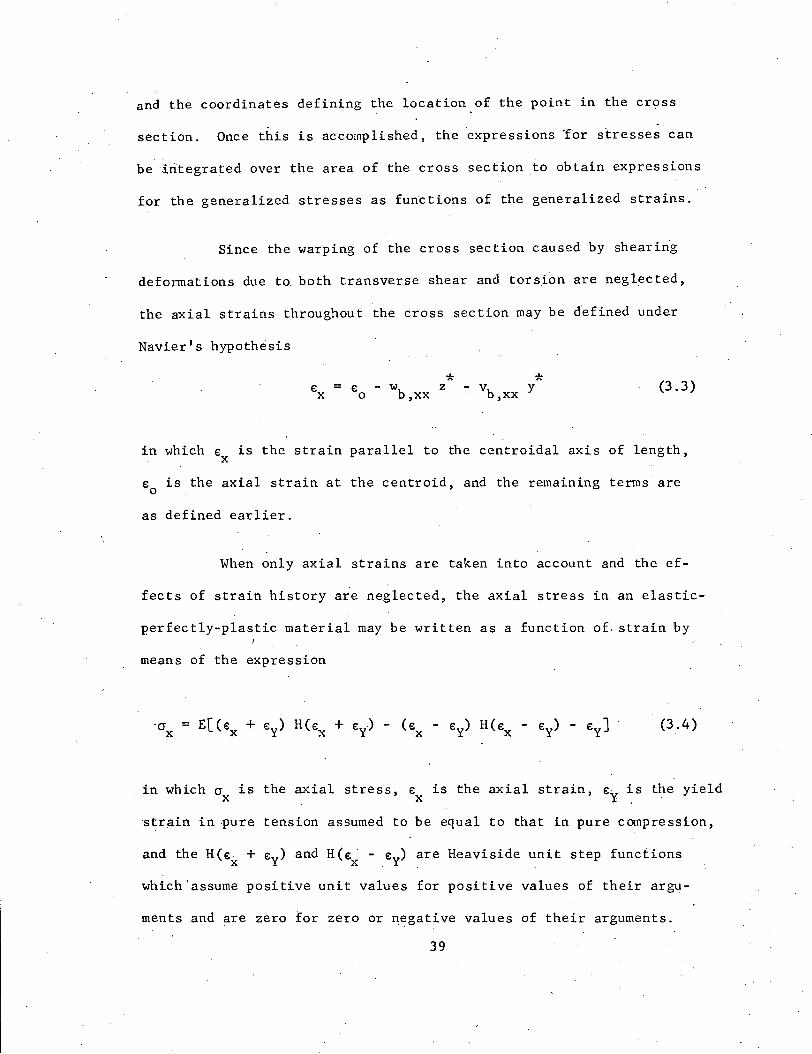
Since the warping of the cross section caused by shearing
defonnations due to both transverse shear and torsion are neglected,
the axial strains throughout the cross section may be defined under
Navier's hypothesis
*- v Yb,xx (3.3)
in which € is the strain parallel to the centroidal axis of length,x
€o is the axial strain at the centroid, and the remaining terms are
as defined earlier.
When orily axial strains are taken into account and the ef-
fects of strain history are neglected, the axial stress in an elastic-
perfectly-plastic material may be written as a function of, strain by
means of the expression
-a = E[(€ + €y) H(€ + €y) - (€ - €y) H(€ - €y) - €y]x X X X X(3.4)
in which ax is the axial stress, €x is the axial strain, €y ~s the yield
'strain in pure tension assumed to be equal to that in pure compression,
and the H(€x + €y) and H(€x - €y) are Heaviside unit step functions
which 'assume positive unit values for positive values of their argu-
ments and are zero for zero or negative values of their arguments.
39
is as follows.
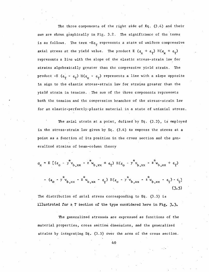
The three components of the right side ofEq. (3.4) and their
-sum are shown graphically in Fig. 3.2. The significance of the terms
The term -Ee represents a state of uniform compressivey .
axial stress at the yield value. The product E (€x + €y) R(€x + €y)
represents a line with the slope of the elastic stress-strain law for
strains algebraically greater than the compressive yield strain. The
product -E (€y - €y) R(€x - €y) represents a line with a slope opposite
in sign to the elastic stress-strain law for strains greater than the
yield strain in tension. The sum of the three components represents
both the tension and the compression branches of the stress-strain law
for an elastic~perfectly~plasticmaterial in a state of uniaxial stress.
The axial strain at a point, defined by Eq. (3.3), is employed
in the stress-strain law given by Eq. (3.4) to express the stress at a
point as a function of its position in the cross section and the gen-
eralized strains of beam-column theory
** * *Ox = E [(€ - Y Vb xx - z w + €y) R(€o - Y V - z w + ey)o ,b,xx b,xx b,xx
* * *- (e - Y Vb xx - z w - € ) R(e - y v -o , b,xx y 0 b,xx*z w -
b,xx
The distribution of axial stress corresponding to Eq. (3.5) is
illustrated for a Tsection of the type considered here in Fig. 3.3.
The generalized stresses are expressed as functions of the
material properties, cross section dimensions, and the generalized
strains by integra~ing Eq. (3.5) over the area of the cross section.
40
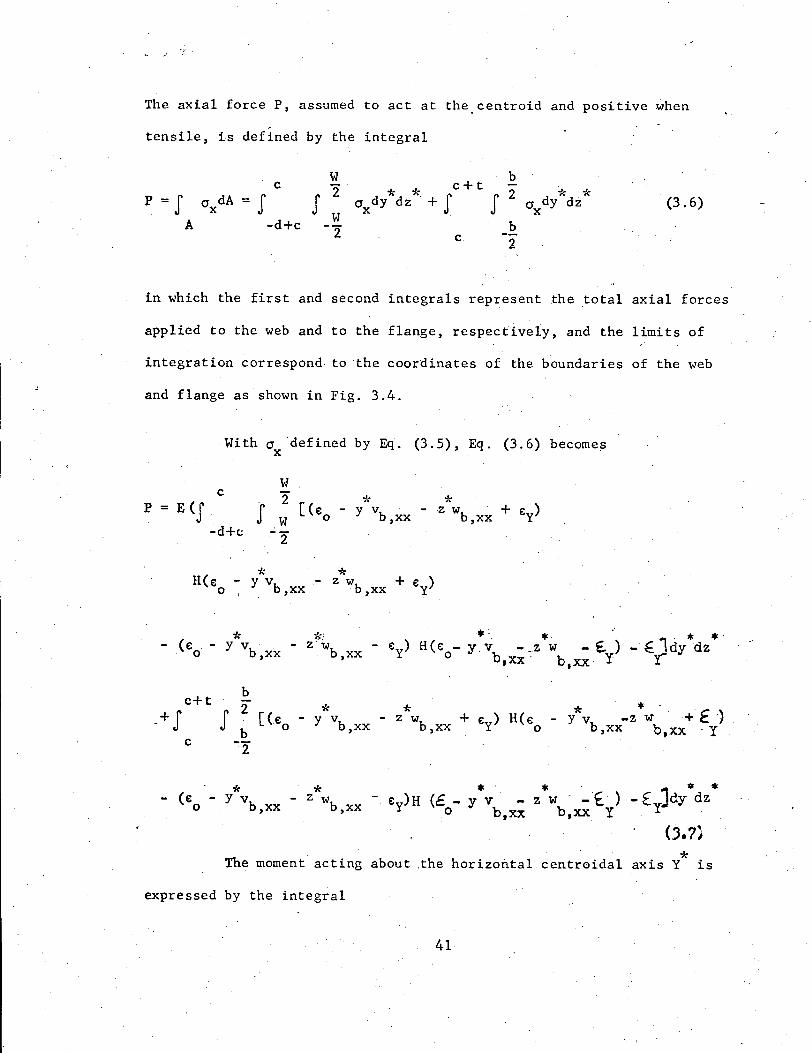
The axial force P, assumed to act at the centroid and positive when
tensile, is defined by the integral
W bc "2 c+t -* * 2 * *p =s o dA = S S o dy dz . +s S Oxdy dz (3.6)x
Wx
A -d+c -2 bc,
2.
in which the first and second integrals represent the total axial forces
applied to the web and to the flange, respectively, and the limits of
integration correspond to the coordinates of the boundaries of the web
and flange as shown in Fig. 3.4.
With ° .defined by Eq. (3.5), Eq. (3.6) becomesx
Wc '2 * *p = E (S S (e - y vb xx - ·z w + ey )
W 0 , b,xx-d+t: -'2
* *. H(e - y v - z w + ey
)o I . b,xx b,xx
* *: .- * . , * *.- (e . - y vb . - z 'tv - e ) H(e - y V - _Z W - E.. ) - ~ 1dy dz
o ,xx b ,xx Y 0 b ,xx - b XX - Y r•
* * * * -- y v - z w + ey ) H(e - Y v -z w+ f·)b ,xx b ,xx 0 b ,xx b, XX - Y
*- (e - Y vbo ,xx*z w -
b,xx* *ey ) H (e - y v· - z w . -£ )
o b,n b,xx Y* *- fyJdY dz
('.7}*The moment acting about ,the horizontal centroidal axis Y is
expressed by the integral
41

* * *My* = J ax (y ,z ) z dA
A
c= E(J
c-d
w
J 2 * *z [( € - Y VI..WO ~,xx
2
- z*W. +E: y ) H(€ - / v. - z*wb + f y ). °,xx 0 0,xx ,xx·
* * * * . .-.* *- (e - Y vb,xx - z W - e:..) H(E: -y vb - z w - E )-fJdy-dz.
o b, xx YO,xx b ,xx Y Y
c+t
+J
c
*z [( E:o
.. , ;
* * .' 11< *-yv -zw +€y)H(E:-~YV -zw +~)
b , xx b ,xx 0" b, xx. b, xx "Y
*" *- (e - y vb . - z w - € ) Ho . ,xx b ,xx y
*and the moment acting about the vertical centroidal axis z is-
expressed by
'1~ * *-cr (y ,z ) Y dAx
c= -E (J
c-d
w
J 2" y"*[ ("" - y*Vb
* * * cw - Z W. + € ) H(E: - Y v. -z w + ~ )W 0 ,xx o,xx Y 0 b,xx b,xx y
-2"
* * * * * *- (eo - Y vb ,xx - Z wb ,xx - E:.t H( €o - Y vb,xx - z ~,xx - ey) - E:yJ dy dz
bc+t
2 -/: * * * *+J J y r (e -y v - Z W + €y) H (E: -y V - Z W +~)
b\.. 0 b,xx b,xx . 0 b,n b,xx.
c -2"
* *- (€ - Y V - z W -o b ,xx b,xx* *E: ) H( € - Y V - Z W . - e:..) -
Y' 0 b ,xx b,xx Y
42.
* *E:) dy dz )
(3.9)

The integration required in Eqs. (3.7), (3.8), and (3.9),. "
which is straightforward but lengthy, is carried out"in Appendix A3,
where the expressions for the generalized stresses and their first
*and second derivatives are listed ~
For the elastic case, these integrals and their derivatives
reduce to
P = EA ub,x
P = EA ub,x ,xx
P = EA U,xx b,xxx
M * = -E1 wY Y b ,xx
M = -E1 wy*,x y b,xxx
(3.10)
(3.11)
(3.12)
'(3.13)
(3.14 )
My*,xx
= -E1 wb
'y ,XXXX
(3.15)
M = E1 vz* z b,xx
M = E1 vz*,x z b,xxx
M = E1 vz*,xx z b,xxxx
* * * *The superscript asterisk on x , y , and zappendix since it serves no useful purposeaxes are ,under consideration.
43/
(3.16 )
(3.17)
(3.18)
has been dropped in thewhen only the deformed

in which A is the area, and I and I are t.he second moments of inertiay z
about the y and z axes of the cross section.
The final generalized stress to be considered is the torsion
T actin"g on the cross section. As noted earlier, the effects of
St. Venant torsion on yielding and the effects of yielding on St. Venant
torsion are neglected. Thus, the St. Venant torsional moment is repre-
sented by the relationship' employed in elastic beam-column theory
T = GI esv ,x(3.19)
in which G is the shear modu 1u s , I is the torsional constant,sv
(bt3 + dW
3) /3 and e x is the rate of change of the rotation of the cross,
section about the shear center. The first derivative of the torsional
moment is given by
T ;; GI e,x sv ,xx
(3.20)
The effect on torsional behavior of warping over the thick-
ness of the plate elements are neglected. As noted by Bleich, these
effects are sometimes significant in a buckling analysis of a T section
13.2
a one. However, it must be kept in mind that the T sections under
consideration here are fastened to relatively heavy plates. Thus, ro-
tation of the cross section is accompanied by bending about the y axis
of the cross section. This bending is essentially the same type of
behavior which provides the primary warping rigidity in wide-flange or
I sections. Therefore, it seems reasonable to assume that the warping
44
over the thickness of the plate e1ements,shou1d prove to be no more
significant for the T section" affixed to a plate than it is in the I
'd f1 'f h' h it . '1 1 d 3.4or w~ e ange sect~ons or w ~c .... ~s customar~ y neg ecte ,
As was the case with the plate differential equations, the
inelastic beam-column differential equations are too awkward to be
written out because of the length and complexity of the expressions
for the generalized stresses. In application, the combination of the
equilibrium equations and the generalized stress-strain law for the
inelastic case is accomplished by means of a digital computer.
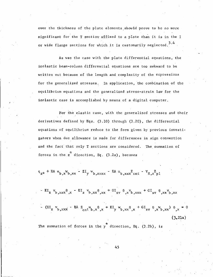
For the.e1astic case, with the generalized stresses and their
deriyatives defined by Eqs, (3.10) through (3.20), the differential
equations of equilibrium reduce to the form given by previous investi-
gators when due allowance is made for differences in sign convention
and the fact that only T sections are considered. The summation of
*forces in the z direction, Eq. (3.2a), becomes
qz* + EA ub wb - EI w - EA u Z - V Z,x ,xx Y b,xxxx b,xxx cnt H,x p1
- EI v e - EI v e + GI e v + GI e vz b,xxx ,x z b,xx ,xx sv ,x b,xxx sv ,xx b,xx
- (EI vb . . - EA Z u e + EI w e + GI e w ) e = 0z ,xxx cnt b,x ,x y b,xx ,x sv ,x b,xx ,x
C3.21a)
*The summation of forces in the y direction, Eq. (3.2b), is
45
qy* + EA u (v + e Z ) - (EI vb,x b,xx ,xx cnt· z .b,xxxxEA Z u e
cnt b ,xx ',x
- EA Z u e - EI w e - EI we + GI e w.cnt b,x ,xx y b,xxx ,x y b,xx ,.xx . sv ,xx b,xx
+ GI e w ) - (-EI w - EA Z u ,- v Z - EI v esv ,x b,xxx Y . b,xxx cnt b,xx H p1 z h,xx ,x
+ Gl sv e xVb xx) e x = 0 (3.21b)" ,
*The summation of forces in the x direction, Eq. (3 .2e), reduces to
EA ub
+ VH
+ (EI wb
+ EA Z ub
+ VHZp1 +EI vb e ) wb,xx . Y ,xxx cnt ,xx z ,xx ,x ~xx
(3.21c)
The torsional equilibrium equation,Eq. (3. 2d), simplifies to
GI e .+ EI w v + EA Z u v - EI v wsv ,xx- y b,xx b,xx cnt b,x b,xx z b,xx.b,xx
= 0 (3.21d)
3.5 Beam Displacements as Functions of Plate Displacements
In order to apply the beam-column theory to the analysis of
grillages or other plate and stiffener systems, the deformations of
the beams mu.st be expressed as functions of the deformations of the
plate. The beam deformations of interest are; 1) ub ' the axial dis
placement.of the centroid and its derivatives through the third order,
46

2) vb' the displacement of the shear center in the direction normal to
the web, and its first through fourth derivatives, 3) wb ' the displace
ment of the shear center in the direction normal to-the plate, and its
first through fourth derivatives, -and 4) e, the rotation of the beam
cross section about the shear center and its first and second derivatives.
The displacements of a longitudinal beam and a transverse
beam are shown in Fig. 3.5. The equations by means of which the beam
deformations are expressed as functions of the plate displacements are
listed at the end of Appendix A.3.
3.6 Resume
The four coupled differential equations of a beam-column theory,
to be applied in the analysis of grillages, have been derived. To this
end the customary assumptions concerning the mode and magnitude of the
deformations of beam-columns have been employed, and the six equations
of equilibrium have been written for a differential element. The six
equilibrium equations have been reduced to the four consistent with a
theory in which transverse shearing deformations are neglected. Then
the usual simplifying assumptions were made concerning the constitutive
relations of steel and a generalized stre~s-strain law applicable to
T sections was developed. Finally, the strain displacement relationship
and the transformations by means of which the beam displacements are
expressed as functions of the plate displacements were presented.
The equilibrium equations, stress-strain law, and the strain
displacement relationships have been combined to obtain the differential
47

'equations for elastic but not for inelastic beam-columns. As is true
with the plate theory discussed earlier, this combination is best ac
complished by means of a digital computer because of the length' and
complexity of the expressions for 'the generalized stresses for other
than the elastic case.
48

4. LOADS AND. BOUNDARY CONDITIONS
4.1 Introduction
The objective of the following sections is the definition of
the loads and boundary conditions required for the analysis of gril-
lages. As noted in Chapter 1, the analysis of the grillage is here
reduced to the analysis of the grillage plate subjected to loads pro-
duced by external agencies and the stiffeners .. For this reason, the
loads and boundary conditions applicable to the grillage plate are
first treated. Then the loads and boundary conditions for the gril-
lage are expressed in terms of the plate loads and boundary conditions.
The only type of load considered to act on the plate at in-
terior points, points not at a beam or a boundary, is the normal load
q (x,y). If it is desired to include the effects of surface tractions
or tangential loads applied at interior points, Eqs. (2.la) and (2.l~)
must contain additional terms X (x,y) and Y (x,y), respectively, to
account for the x and y components of such loads in the equilibrium
d.. 2.1con ~t~on.
4.2 Loads Applied by Beams
The equations of equilibrium of plate-beam junctions are
employed to define the loads applied by the grillage beams to the
grillage plate. They are also used to express the force boundary
conditions for grillages. Two types of junctions must be considered;
one - the junction of a plate differential element with a single beam
49
differential element, and the other - the junction of a plate differ-
entia1 element ~ith two intersecting beam different~al elements:
4.2.1 Junction of Plate and a Single Beam'
The differential equations of equilibrium of a beam-column
differential element written'in Chapter 3 become the equations of
equilibrium for a junction of a plate differential element and a
single beam-column differential element when the loads q ., q ., VH
,y';( z';'('
and Mp1
(Fig. 3.1) are expressed as discontinuities or jumps in the
plate generalized stresses, as shown in Fig. 1.3. Thus, all that
need be done here is to express these load terms as discontinuities
in the plate generalized stresses. The treatment given here is es-
sentially an extension of a simplified approach employed by Kusuda in
a buckling analysis of stiffened p1ates. 4 . 1 Kusuda directly considered
only the form of plate beam reaction corresponding to the beam loads qz*
and M l' He neglected the q oJ. and included the V indirectly by employ-p yn H
ing an effective width of plate in the definition of beam properties.
The distributed load qy* acting on a beam corresponds to an
in-plane line load applied to the plate. This in-plane line load may
be represented, as shown in Fig. 1.3, by a discontinuity in the ap-
propriate axial or "membrane" force in the plate. Thus, for a trans-
. verse beam
= oN' = N +qy* Y Y
and for a longitudi.nal beam'
50
Ny (4.1)
= -eNx
= Nx
N +x
'.
(4.2)
The terms eN and eN represent the jumps or steps in they x
plate in-plane forces Nand N , respectively, occurring at the beams.y x·
They are readily isolated and expressed directly as functions of the
constant coefficients of the plate displacement functions as long as
the plate remains elastic. For a yielded plate, however, it is more
convenient to evaluate the jumps by determining numerical values of
the in-plane forces at arbitrarily small distances on opposite sides
of the beam and taking their difference. For example,
eN = N +Y Y
NY
(4.3)
withN + and N the in-plane force N evaluated on the positive andy y y
negative y sides of the beam, respectively. Introduction of the defi-
nition of the beam loads, given inEq. (4.1) or Eq. (4.2), into the
equilibrium equation of a beam differential element (Eq. (3.2b» may
be regarded as a definition of the load applied ta the beam by the
plate, or as desired here, a definition of a load applied to the
plate by the beam. In the description to follow, the superscript plus
indicates the positive x side of a longitudinal or the positive y side
of a transverse. The superscript minus indicates the negative x. side
of a longitudinal or a negative y side of a transverse.
The distributed axial load VH
which acts on the beam cor
responds to an in-plane line load acting at the plate middle surface
which may be represented as a discontinuity in the in-plane shear
51

force N , as shown in Fig. 1.3. For a transverse beam, VH
may pexy
defined
= oNyx= N +
yxNyx
(4.4)
and for a longitudinal beam, VH is defined
= oN = N +xy xy Nxy (4.5)
The values of VH
, given by Eqs. (4.4) or (4.5), serve to define the
variable axial load acting on a transverse or longitudinal beam, re-
spec~ively, in Eqs. (3.2b) and (3.2c).
The derivative of the variable axial load required in
Eq. (3.2a) is, for a transverse beam
+v = oNH,x· yx,x
and for a longitudinal beam
= Nyx,x
Nyx,x
(4.6)
+VH,x = oNxy,y = Nxy,yNxy,y (4.7)
The load applied normal to the plate by a beam, qz* in the
beam differential equations, Eq. (3.2a), corresponds to a line load
on the plate which may be represented as a discontinuity in the trans-
verse shear force V or Vyz XzFor a transverse beam
+= ·oVyz+::M
y,y .. 2Mxy,x
My,y + 2Mxy,x (4.8)

+ +
and for a longitudinal beam
Mx,x 2Mxy,y Mx,x + 2Mxy,y (4.9)
The distributed torque Mpl
acting on a beam corresponds to
a discontinuity in the plate bending moment over the beam. For a
transverse beam, this discontinuity in moment is
=-eMy+ -= -M + M
Y Y(4.10)
and for a longitudinal beam, the discontinuity in plate moment is
= eM = M +x. x
Mx
. (4.11)
The value o~ M l' given by Eq. (4.l0).or Eq. (4.11), is employed in.p
Eq. (3.2d) to define the distributed couple appli~d to the plate by
the beam.
The form of plate-beam interaction corresponding to a dis~
continuity in the plate twisting moment at a beam is not considered
per se. The discontinuity in plate twisting moment is, however, in-
directly taken into account by means of the definition of the trans-
verse shears V and V employed in Eqs. (4.8) and (4.9). As dis-yz xz
cussed by Timoshenko (page 84 of 2.1) or Love (page 450 of 2.4), the
definition of the transverse sheqrs V . and Vxz~ employed inyZ"K. ..
Eqs. (4.8) and (4.9) is such that. they are made statically equivalent
in effect to the transverse shears Q and Q acting with the twistingy. x
53

Since the twisting'moment in an elastic
moments M and M by subtracting the gradients of the twisting mo-xy yx
ment from the Q's.
It is readily demonstrated that the plate twisting moment
in an elastic plate of uniform thickness exhibits no discontinuity at
a beam and thus need not be c~nsidered at all in a plate theory in
which transverse shearing deformations are neglected. The logic lead-
ing to this conclusion is as follows. In a plate theory. in which
transverse shearing deformations are neglected, the displacement wand
its first partial derivatives wand w must be single valued. It,x ,y
can be shown that a necessary condition for wand its first partial
derivatives to be .single valued is that the mixed partial derivative
b . 1 1 d 4.1w . e s~ng e va ue .,xy.
plate is defined" by the product of-a plate constant and the mixed
partial deri~ative w _ , it must be single valued throughout the plate,,xy
even at a-beam, if transverse shearing deformations are neglected.
Since' the partial derivatives wand thus the plate,xy
twisting moments are single valued for the elastic case at a plate
beam junction, their derivatives with respect to an axis parallel to
the beam must be as well. That is,M must be single valued at axy,y
longitudinal beam, and similarly H must be single valued at a_ . xY,x
transverse beam. Thus, the discontinuities in transverse plate
shears at a beam, Eqs. (4.8) and (4.9), can be defined entirely in
terms of the discontinuities in ~he derivatives of the bending mo-
ments, which can exhibit the requisite jumps.
54
The argument concerning the discontinuity in plate twisting
moment no longer holds true after the plate yields a·t the plate':':beam
junction. As can be seen in Eq. (2.l0c), the plate twisting moment
is also a function of the membrane· strains and the curvatures w. ,xx
and w for this case. Since these functions can be discontinuous,yy
at a beam, the twisting moment for an inelastic plate can as well.
However, since the plate twisting moment is small relative to the
beam bending moments and the discontinuity in twisting moment after
yielding is apt to be even smaller, the way in which this effect is
taken into account should not be important.
4.2.2 Junction of a Plate and Two Beams
The equilibrium equations for the junction of two beams may
be regarded as constraints in addition to the constraints afforded by
plate theory to the solution functions representing plate displace-
ments. Alternatively, they may be thought of as special cases of
plate-beam equilibrium equations considered in the previous section.
If the latter concept is employed, it should be interpreted in light
of the fact that discontinuities in the beam generalized stresses
cannot be resisted by corresponding singularities in the plate gen-
eralized stresses. Thus, the equilibrium equations at the junction
of two stiffeners, which entail considerations of discontinuities
of beam stresses, are formulated solely in terms of the beam gener-
alized stresses.
The logic behind this conclusion is illustrated with the
aid of Fig. 4.1. There the junction of two beams and the adjacent
55
prirtion of the plate are shown as they actually appear. In Fig. 4.lb
the middle surface of the gri~lage plate and the pl~te elements~of the
grillage beams are shown. This is the appearance of the junction when
so idealized that only the behavior of the middle surfaces need be
considered. Figure 4.lc shows the one-dimensional junction element
for which the joint equilibrium equations are actually written. This
one-dimensional junction element is a rigid line defined by the inter-
section of the middle surfaces of the web plates of the two beams.
The apparent rigidity of the line is a consequence of assuming that
plane sections remain plane and normal to the deformed longitudinal
axes in both beams.
The forces and couples shown on the line representing the
beam junction in Fig. 4.lc are the finite changes in the beam gener-
alized stresses assumed to occur over an infinitesimal length in
each beam. The plate generalized stresses are distributed forces and
couples. Since they act over an infinitesimal length and are finite
in magnitude, they do not enter into the equilibrium equations written
for a beam junction idealized in this fashion. An exception to this
. 2.1would be the concentrated corner forces called R by Timoshenko.
These forces act at the corners of plates accarding to thin plate
theory (transverse shear deformations are neglected). The Rls are
equal to twice the twisting moment acting in the plate on opposite
sides of a beam and can be shown to be self-equilibrating'
at all but the corner beam junctions as long as the plate remains elas-
tic and smoothly continuous. This follows from the same logic employed
to justify. neglecting the discontinuity of the elastic plate twisting
56

moment at a beam. It is assumed that the difference in the R's sub-·
sequent to yielding is small ~nough compared to the changes in beam
shear at a joint to justify neglecting any such difference for in-
elastic plates as well.
The six equations of equilibrium for the beam junction are
written in terms of the discontinuities 0 in beam stresses as follows.
The subscript T or L indicates whether the discontinuity occurs in a
transverse or longitudinal beam. The equation of equilibrium of
forces in the directions of the deformed x axis is
OPT - oV. = 0y«L(4.12a)
The equation of equilibrium of forces in the direction of the deformed
y axis is
ePL - ev . = 0y-l;T (4.12b)
and the su~~ation of forces in the direction of the deformed z axis is
~V + eV = 0U z-/;L z-/;T (4,12c)
Equation (4.12c) contains an additional term R for a corner beam junc
**tion. Summation of moments about the x axis of the transverse beam
gives
eTT - eMY*L + ePL (dT + 0,5 t T - dL + c L) = 0
57
(4.12d)
**The summation of moments about the x a~is of the longitudinal. beam
is
(4.l2e)
and the summation ·of moments about the deformed z* axis of the joint is
&Mz*T + &Mz*L = 0 (4.12f)
Equations (4.12) are written under the sign convention that a c-beam
generalized stress is equal to the value on the negative side, in
terms of the beam axis, subtracted from the value on the positive
side. As is true for the discontinuities in plate stresses discussed
earlier, thp. discontinuities in the beam generalized stresses can be
readily expressed for the elastic case as functions of the discon-
tinuities in the derivatives of the beam displacements .. For the
inelastic case, however,the discontinuities are most readily evaluated
by determining the values of the generalized stresses at arbitrarily
small distances on the positive and negative sides of the joint and
taking their differences.
4.3 Force Boundary Conditions
The equilibrium equati~ns'written in the preceding sections
may be employed to express the bO\lndary conditions fora grillage sub-
jected to pure force boundary conditions, that is, subjected to speci-
fied edge' reactions but not constrained to deform to a given shape at
58

the edges. In order to express the boundary conditions by means of
these equilibrium conditions in this case, the state of stress at
the boundary must be completely defined. That is, the generalized
stresses for projecting infinitesimal plate and beam elements just
at the periphery of the grillage must be given in their entirety.
It is not sufficient to specify a system of forces applied to the
grillage as a whole without specifying how they are applied to the
individual boundary beam and plate elements. This is in distinct
contrast to the manner of specifying force boundary conditions in
the simplified methods of analysis currently in use. It reflects
the fact that fewer and less restrictive assumptions are herein made
concerning the interaction of the structural elements of the grillage.
Pure force boundary conditions are difficult to apply in
the most general case. It is ~ifficult, if not impossible, to
specify a physically realizable set of grillage edge forces for
other than a reaction free edge. The difficulty arises in at
tempting to specify edge forces which are of such magnitudes that
1) the individual elements of the grillage are strong enough to
withstand them and 2) the ultimate strength of the grillage is not
exceeded.
The generalized stress-strain laws developed in Chapters
2 and 3 can be employed to produce the data required to determine
the limiting combinations of axial forces and bending moments for
a beam cross section and comparable limiting combinations of the
generalized stresses on a plate differential element; Then the
59
boundary forces can be checked to ensure that these limits are not
exceeded.
The possibility that a specified set of edge forces is in
excess of the ultimate strength of the grillage is more difficult to
circumvent. A possible approach would be to try various combinations
of edge forces to see if a solution could be obtained. An approach
of this nature would obviously be costly in computation time.
For cases for which it is possible to do so, imposition of
force boundary conditions is accomplished as follows. For a grillage
with edge beams, the known edge reactions are introduced into the
equations of equilibrium written for plate-beam junctions as if they
were the generalized stresses acting in the grillage elements con-
tinued. For example, at a point on an edge transverse between two
longitudinals the tern 6N is definedy
6N = N +Y Y
NY
(4.13 )
the grillage.
with N + the given edge reaction and N - the edge reaction computed byy y
means of the generalized stress-strain law at the positive y end of
At the negative y end of the grillage, N + is computedy
by means of the generalized stress-strain law and N is the giveny
edge reaction. In a similar fashion, the joint equilibrium equations
are employed at a boundary junction of a longitudinal and a transverse.
For a grillage without edge beams; the edge values of the plate and
beam generalized stresses need only be equated to the given values.
60

The sign convention for edge r~actions is the same as· that
employed for the generalized ~tresses. For example, a positive in
plane bo~ndary force applied to the plate would induce tension, etc.
It should be noted, at this point, that the solution technique
to be emplo~ed here (see Chapter 6) can be used directly to handle only
pure force boundary conditions. Thus, if there are displacement or
mixed boundary conditions· to be satisfied they must be 1) such that
all of the displacement functions selected identically sa~isfy the
displacement boundary conditions, or else 2) they must be employed in
a separate operation to express some of the constant coefficients as
functions of the others. In the latter case, it would be in keeping
with the collocation technique employed here to require that the dis
placement boundary conditions be satisfied at a finite number of
points. The equations employed to express some of the constants as
functions of the others can be derived by equating the displacements
at these points to the known or given values.
61
The only form of pure displacement bo~ndary condition treated
in this ir:tvesti'gation isa cqmbination of fixed-end' conditions for
bending and sp~cified straight line in-plane boundary deformations.
This combination is one of the simpler to treat since it can be
accomodated by displacement functions which identically satisfy the
boundary conditions.
4.5 Mixed Boundary Conditions
Mixed boundary conditions must, of course, be treated by
employing the methods employed for force and displacement boundary
conditions discussed in the preceding sections. 'That is, the dis
placement boundary conditions must be employed to express some of
the constant coefficients as functions of the remainder if the func
tions cannot be selected to identically fulfill the specified dis
placement requirements. Then, the boundary equilibrium equations
corresponding to the appropriate force boundary conditions are
employed. The difficulties noted concerning pure force boundary
conditions are equally troublesome for the mixed boundary value
problems.
4.6 Resume
The loads applied to the grillage plate by external agen
cies to be treated here have been discussed. The loads applied by
the grillage beams have been defined in terms of the generalized
stress-strain laws.for plates and beams developed in Chapters 2
'.
and 3 and the beam differential equations derived in Chapter 3. The
treatment of boundary conditions and problems associpted with actually
applying them have been briefly discussed.
63

5. THE DISPLACEMENT FUNCTIONS
5.1 Introduction
The functions selected to describe the three components of
displacement of the grillage plate must be such that they can; 1) sa
tisfy the plate and beam-column differential equations derived iri the
preceding chapters, 2) provide the requisite discontinuities in the
plate generalized stresses at plate-beam junctions and in the beam
generalized stresses at the junction of two beams, 3) satisfy the re
quirements imposed by the boundary conditions, and 4) satisfy the re
quirements of compatibility in the plate and in the beams. In the
following sections the characteristics to be exhibited by the displace
ment" functions in order that they fulfill these requirements are de
lineated, and the functions selected t6 provide these ~haracteristics
are presented.
5.2 The Form of the Displacement Functions
It is assumed that displacement functions of the type that
satisfy the differential equations of elastic beam-column and plate
theories will prove to adequately define the displacements when the
effects of inelastic behavior are taken into account. This assump
tion constitutes a tacit neglect of the requirements for discontinui
ties in the second and higher order derivatives of the in-plane dis
placement functions and comparable discontinuities in the third and
higher order derivat ives of the bending displacement func t ion which
result from the discontinuity in s~ope of the bilinear stress-strain
law employed.
64

The general form of the solution function employed to define
one of the components of displacement of a beam-column is the sum of
a low order polynomial and infinite series of circular and hyperbolic
f . f h d' 3.2,3.3,3.4unctions 0 t e coor inate x. . No comparable general form
of solution is available for the plate differential
. 2.1,2.4,4.1,5.1 fl' f . h' hequations. .However, a type 0 so ution unction w 1C
has proven to be satisfactory for many plate problems is a product
function of the form
f(x,y) =n mL: L:
i=l j=lA.. X.(x) Y.(y)
1J 1 J(5.1)
in which f(x,y) is a component of displacement to be expressed as a
function of x and y, X.(x) and Y.(y) are functions1 J
. 1 d A ff" 2.1,2.4t1ve y, an .. are constant coe 1C1ents.1J
ofx and y, respec-
The X. and Y. are1 " J
functions of the type appearing in the solution to the beam-column
differential equations. That is, they are the terms of low order
polynomials and infinite series of circular and hyperbolic functions
in x and y. The infinite series must, of course, be truncated for
purposes of obtaining numerical results.
The three components of displacement of the grillage plate
are expressed as product functions of the form shown in Eq. (5.1).
Since it is apparent that the pattern of displacement is roughly re-
peated from panel to panel in the grillage, the hyperbolic functions
are omitted. Then, the X. and Y. are the terms of low order poly- ,1 J .
nomials and truncated trigonometric series. The requirements imposed
on the functions defining the displacement w normal td the surface of
65
the plate, and the functions u and v defining the in-plane disp1ace-
ments of the plate differ in detail, Thus, they are. presented se-
parate1y in the following sections.
5.3 Characteristics Required of the Bending DisplacementFunctions
The bending displacement w, normal to the middle surface of
the plate, must fulfill the requirements of compatibility as well as
the requirements of equilibrium. The requirements of compatibility
for bending deformations imposed by consideration of plate behavior
are that the displacements be smoothly continuous.2
.l
That is, the
function 'Wand its first partial derivatives must be single valued.
As noted earlier, the requirement that the first partial derivatives
wand w be single valued implies that the mixed derivative w,x ,y ,xy
must also be single va1ued. 4 . 1 ,5.l
The requirements of compatibility of deformation between
the two beams at a beam junction impose restrictions on b9th the
bending and in-plane components of displacement of the plate. Fu1-
fillment of the conditions that w ,w ,and w be single valued,,x ,y ,xy
required by considerations of plate behavior, ensures that the com-
ponents of beam displacements due to bending displacement of the plate
fulfill the requirements of compatibility. The conditions to be im-
posed on the in-plane displacement functions are discussed in
Section 5.5.
The requirements of equilibrium at the junctions of plates
and beams'"make necessary certafn characteristics in the second and66
higher order partial derivatives of the ?isplacement function w.. In
order for .the r~action between the plate and abeam ~orresponding to
a distributed torque on the beam to be possible~ the plate must
exhibit a discontinuity in bending moment as it passes over the beam.
The bending moments, as indicated by Eqs. (2.l0a) and (2.l0b), are
defined by a product of f2i
, in general, a nonlinear function of
the generalized strains, and a linear function of the curvatures.
Thus, the discontinuity in bending moment may be produced by a dis
continuity in either the function f2i
or one of the curvatures.
For elastic plates of uniform thickness, the function f2i
is a constant. Therefore, the discontinuity in bending moment must
be due to a discontinuity in one of the curvatures. In a prod~ct
function, as employed here, a discontinuity in curvature of a line
parallel to the axis of length of the beam is impossible when the
function is constrained to be smoothly continuous. Thus, in order
to introduce the discontinuity in bending moment of an elastic plate
passing over a beam, the displacement function w must be capable of
exhibiting a discontinuity in the second partial derivative with
respect to the axis normal to the beam. Such a discontinuity can
be introduced only by employing a function of the dimension normal
to the beam axis which contains the required discontinuity in its
second derivative.
As noted above, the discontinuity in f2i
may provide the
necessary discontinuity in plate bending moment at a beam after the
plate yields. Since f2i
is a function of all of the generalized
67

strains, the requisite discontinuity in bending moment can be intro-
duced by means ,of a discontinuity in anyone of the.generalized-
strains. Thus, the discontinuity in curvature of a line normal to
the axis of the beam is a characteristic which is sufficient to
cause but does not necessarily accompany the discontinuity in plate
bending moment. An argument similar to the foregoing, concerning
the necessity for the discontinuity in strong axis bending moments
in the beams at cross beams, leads to the same conclusion regarding
the necessity for a discontinuity in the second partial derivatives
wand w at the longitudinals and transverses, respectively, for,xx ,yy
the elastic case.
In order for the reaction between the plate and a beam
corresponding to the beam load qz* of. Chapters 3 and 4 to be possible,
the plate t~ansverse shear must exhibit a discontinuity, called oV orx
oV in Chapter "4, at a beam. By employing essentially the same logicy
used earlier with regard to the discontinuity in plate bending mo-
ment, it can be concluded that for an elastic plate of uniform thick-
ness, the third partial derivative of w with respect to the axis nor-
mal to the beam must be discontinuous at a beam. That is, w must,xxx
be discontinuous in x at a longitudinal beam and w must be dis-,yyy
continuous in y at a transverse beam. This discontinuity in the third
partial derivative of w at a beam is a sufficient but not a necessary
condition for an inelastic plate, because discontinuities in the other
generalized plate strains can introduce discontinuities in f2i
and its
first derivative.
68
5.4 Functions Employed to Define the Be~ding Displacement
'The trigonometric functions employed to define the displace-
ment normal to the surface of the plate as functions of x are of the
form
and
w.(x) = 0.5 (1 _ cos 2iTI x)1 X
maxi = 1,2,3 --- (5.2)
w. (y)J
2j TI y)0.5 (1 - cos ~y~-~
maxj = 1,2,3 --- (5.3)
in which X and Yare the width and length of the grillage. Ifmax max
it is so desired, these functions may be expressed in the alternate
form
and
w. (x)1
i TI X- sin2X
maxi = 1,2,3 --- (5.4)
w. (y) = sin2
J
j TI YYmax
j = 1,2,3 --- (5.5)
The functions given in Eqs. (5.2) and (5.3) can be employed
in a product ~unction to represent a bending displacement w roughly
of the type expected of a grillage with fixed edges. At the boundary
both wand its first derivative normal to the boundary are zero, and
the second and higher order derivatives are non-zero. They are,
69
however, smoothly continuous and cannot provide the jumps in curvature
required at the'p1ate-beam jupc tions.
To introduce the requisite jumps in curvature at the beams,
two additional functions are employed for each grillage beam. Func-
tions of this type are derived by multiplying low order polynomials,
with coefficients selected to ensure compatibility, by step functions
with zero arguments at a beam. One such function of ~ is
([ - 2K 2 K(~ +-.£)
X Xo 0
2+ (X. "- x) H(x - X ))/W1mD 0 mD
and the other, similar in form, is
(5.6)
(2K 3 + 3K 2) x3 +
o 0
+ (Xmax3
- x) H(x - X ))/W2o max(5.7)
in which X is the ordinate of a longitudinal beam, X. is the gri1-o max ...
1age width, K is X Ix - 1, and W1
and W2
are the maximumo max 0 max max
ordinates of functions w1
and w2
' r~spectively.
The maximum values of the functions occur at
tor w1
and at
x = Xo
X 2o
3Xmax
70
(5.8)

x xo
X 2o
(2X +.X )max 0
, (5.9)
Functions Wi and \012
can be employed to represent fixed edge
displacement functions since they and their first derivatives are'
zero at x = 0 and x = Xmax
Their first derivatives are continuous,
but their second and higher order derivatives exhibit discontinuities
at,x = XO' Thus, they may be employed to introduce the discontinuities
in plate and beam bending moments and shears.
To permit the treatment of bending displacement boundary
conditions other than the fixed edge condition, two functions which
are non-zero at x = 0 and two which are non-zero at x = X may bemax
introduced in the form
w(x)
w(x)
w(x)
w(x)
3X -x
= (max )Xmax
2X -x= (max)
Xmax
3= (_x_)
Xmax
2= (_x_)
Xmax
(5.10)
(5.11)
(5. 12)
(5.13)
in which all terms are as defined earlier.
The functions in yare of the same form as those given in
Eqs. (5.3) through (5.13), with ,y's introduced in place of XIS.
71

II
L
5.5 Characteristics Required of In-Plane DisplacementFunctions
In order that the structural integrity of the plate be main-
tained, the functions u(x,y) and v(x,y) must be single-valued. This
condition implies that u be continuous in x and v be continuous,Y ,x
in y throughout the plate.
The remaining conditions imposed by considerations of com-
patibility are those needed to maintain structural integrity in the
beams. The weak axis bending displacement of a beam, it will be re-
called, is a function of the in-plane plate displacement normal to
the axis of the beam and the first partial derivative with respect
to the axis normal to the beam of the bending displacement. Thus, to
ensure that the first derivative of the weak ~xis beam bending dis-
placement with respect to the axis of length of the beam is single-
valued, as required in a beam theory in which shearing deformations
are neglected, the quantities u or v and w must be single-- ,y ,x ,xy
valued at longitudinal or transverse beams.
The conditions that u and w be single-valued in y at,y ,xy
a longitudinal beam may be interpreted to mean that the longitudinal
beam may not exhibit kinks (discontinuity of slope) in a plane
parallel to the plane of the plate. Similarly, the requirement that
v and w be single-valued in x at a transverse simply expresses,x ,xy
the condition that the transverse beams may not exhibit kinks. These
restrictions, inherent in the form of beam theory here employed, would
not apply if transverse shearing deformations of the beam were taken
into account. However, when transverse shearing deformations are
72

neglected, kinks imply infinite curvature and thus infinite strains
and cannot be permitted.
In order that complete compatibility of deformation between
the two beams be maintained at a heam junction, 1) both beams must
. rotate through the same angle about all three coordinate axes and
2) for a point common to both beams, the components of displacement
of one beam must equal the components of displacement of the other.
The restrictions imposed on the displacement functions up to now en-
sure that the rotations about the two horizontal axes X and Yare
equal in the beam, and the three components of displacement are equal
at the point where the center lines of the webs of the beams intersect
the !Uidd1e surface of the plate.
If it is desired to ensure that the rotations of both beams
about the z axis are equal, the following additional condition, derived
by equating the vb . of the two beams, must be satisfied:,x
w,xy
v ,x + u ,y (5.14)
This condition is a consequence of the assumption of complete rigidity
of the junction of the two beams. It reduces to an obviously fal-
1acious requirement if a limiting case is obtained by reducing the
beam depths to zero. For this case, the requirement expressed by
Eq. (5.14) would be that the sma1~ displacement definition of shear
strain be equal to zero. For this reason, this requirement is neg1ect-
ed.
73

The first partial derivatives of the in-plane displacements
with respe~t to'the axes norm~l to the axes of length of the beams
must be capable of exhibiting discontinuities at the beams. That is,
u and v must be capable of exhibiting a discontinuity in x at,x ,x
each longitudinal beam and v and u must be capable of exhibiting,y ,y
a discontinuity in y at each transverse beam. The necessity for
these discontinuities can be demonstrated by means of essentially
the same logic employed earlier to demonstrate the necessity for dis-
continuities in plate curvature at the beams. Discontinuities in the
first partial derivative of the in-plane displacement normal to the
beam with respect to the axis normal to the beam correspond to jumps
in the in-plane forces normal to the beam. Discontinuities in the
derivative with respect to the axis normal to the beam of the dis-
placement parallel to the beam correspond to discontinuities in
shears tangential to them.
One final possible requirement concerning the characteristics
required of the in-plane displacement functions can be extracted from
a consideration of the behavior of the beams. The beams are expected
,""""to be capable of exhibiting a discontinuity in weak axis bending mo-
ment at the junction of two beams. To achieve this for a longitudin-
al beam in the elastic case, wand/or u must be discontinuous,xyy ,yy
in y at the junction of a longitudinal and a transverse. Similarly,
wand/or v must be discontinuous in x at a junction of two,xxy ,xx
beams i£ a transverse beam is to exhibit a discontinuity in weak axis
bending moment. If the displacement function w(x,y) could not be
selected such that wand w . exhibit these discontinuities, then,xyy ,xxy
74
u(x,y) and
w(x,y) ha~
v(x,y) must be so selected that u and v do. However,. ,yy ,xx
been' selected such. that w can exhibir a jump at a 10ngi-,xyy
tudina1 beam and w can exhibit a jump at a transverse. Thus, the,xxy
required jump in weak axis beam moment may be accounted for without
the jump in u and v,yy ,xx
5.6 Functions Employed to Define In-Plane Displacements
As done with the bending displacement, the in-plane disp1ace-
ments are represented by three types of functions: 1) truncated trigo-
nometric series, 2) products of step functions and low order po1y-
nomia1s to introduce the requisite discon~inuities in the generalized
stresse.s, and 3) low order polynomials to introduce the effects of
boundary displacements. The low order polynomial employed to describe
in-plane displacements are linear functions.
The in-plane displacement in the x direction, u(x,y), is re-
presented by functions of x and of y as follows. The terms of the
trunca ted trigonometr ic ser ies emp 10yed are
and
u. (x)~
u. (y)J
2iT i x= sin --X
max
= cos 2iT j yymax
75
(5.15)
(5.16)

The products of linear functions and step functions in x
employed to introduce the discontinuities in plate and beam general-
ized stresses at the beams are of the form
u. (x)~
x - x= xx. H(X; - x) + ~xm~ax_·__--;:x,- H(x - X.)
~... max i ~(5.17)
in which X. is the x coordinate of a longitudinal beam and the re~
maining terms are as defined earlier. One term of this type must be
employed for each interior longitudinal beam in order to introduce
the discontinuity in N at the longitudinal.x
The sel~ction of comparable terms in y offers difficulties
because of a conflict between the requirements imposed by consider-
ations of equilibrium and those imposed by considerations of compati-
bility. As discussed earlier, to fulfill the requirements of equili-
brium at a transverse beam, N must be capable of exhibiting therexy
a discontinuity in y and thus, either u or v must be discon-,y ,x
tinuous in y at a transverse. The latter possibility mus~ be excluded
Thus,in order to ensure compatibility in the plate. u must be,y
capable of exhibiting a discontinuity in y at a transverse beam. Yet,
u must be continuous in y at a longitudinal beam in order to 'ensure,y .
compatibility in the longitudinal.
To resolve this difficulty, functions in y of the same form
as those employed in x, Eq. (5.17.), are employed
Y - Yu.(y) =.L H(Y. - y) + max Y H(y _ Y.)
J ' Y. ~ Y - ~J max i
(5.18)
76
.'
in which Y. is the y coordinate of the jth tra~sverse, in order to inJ
troduce the required disconti~uity in u at a transverse. They are,,y
however, used only in conjunction with terms u(x) which have zero
values at the longitudinals, that is, the higher order sine terms.
This limits the applicability of this particular combination of func-
tions to grillages in which the longitudinals lie on lines which are
at rational fractions (quotients of integers) of the width in order
that sine terms with zero values at the longitudinals exist~
The four functions, two in x and two in y, introduced to
permit consideration of in-plane displacement and force boundary con-
ditions are
ul
(x) = 1 -x
Xmax
u2 (x) x= --Xmax
u l (y) = 1 - -.L-Y
max
u2 (y) -y-Ymax
(5.19)
in which all terms are as defined earlier.
The functions employed to define the in-plane displacements
in the y direction, v(x,y), are of the same form as those defining
u(x,y) except that the functions of x in u become functions of y in
v and the functions of y in u are functions of x in v. Thus, the
functions employed are also limited in applicability to grillages in
.77

which the transverses lie on lines which are at rational fractions of
the length of the grillage.
5.7 Combination of the Product Functions
The terms of the displacement functions are combined in the
following fashion:
fbi (y) ,II
f(x,y) = [fbi(x)--- fdj(x)--- ftk(x)---]Anm fdj(y)", I
I
f~k (y)
(5.20)
The fbi (x) are the terms employed to introduce the boundary displace-
ments at x = 0 and x = XmaxTwo such terms are required for u or v
and four are required for w. The fbi(y) are the comparable terms in
y. The fdj(X) are the terms employed to introduce the discontinuities
in stresses at the longitudinals. One such term is required for each
longitudinal beam in u or v and two are required for W.· The fdj
(y)
are the comparable terms in y required to introduce discontinuities
in stresses at the transverses. The ftk(x) and ftk(y) are the tri-
gonometric terms in x and y, respectively. There are to be a total
of n terms in x and m terms in y. Combination of the terms, 'as shown
in Eq. (5.20), offers the advantage of permitting the analyst to
determine quickly the nature of the terms corresponding to given
constant coefficients.
5.8 Resume
.,~,The characteristics to be shown by the displacement func-
tions in order that the requirements of equilibrium and compatibility
78

be satisfied have been discussed .. Solution functions which exhibit
these character~sticshavebeen presented and the manner in which they
are to be combined described. Attention can now be directed to the
technique by means of which the constant coefficients of the displace
ment functions can be evaluated.
79
6. PROPOSED METHOD OF SOLUTION
The constant coefficients of the displacement functions are
to be evaluated by means of a variant of the method of·collocation
adapted for computer application. In the following sections collo-
cation is first described in general terms. Then the specific mode
of application of the method is outlined and a simple example which
lends itself to a geometric interpretation is presented to illustrate
the technique. Then a more de tailed description of the method and" its
application is presented and a more realistic example is worked.
6.1 The Method of Collocation
The method of collocation in its simplest" form consists of
evaluatihg the constant coefficients of a set of solution function so
that a differ~ntial or integral equation is satisfied at a finite
b f ." "6.1, 6.2 1 h h d h f 1num er 0 po~nts." To app y t e met 0 in t is orm to a sing e
differential equation, n functions which identically satisfy all boun-
dary conditions are first selected and multiplied by unknow~ coefficients.
Then the differential equation is written for each of n points to obtain
a set of n equations which are solved to evaluate the coefficients of
the solution functions.
If a set of functions which identically fulfill the boundary
conditions of the problem is not available, the collocation concept may
also be applied to the boundary conditions. If, for example, it is
desired to employ n solution functions and satisfy a singly boundary
condition at each of m points, the m equations expressing the boundary con-
ditions are written for each of the m boundary points and the differential
80
equation is written forn-m interior points to obtain n equations for the
n unknown constant-coefficients.
Since the differential equation or equations are satisfied at
the interior points at which collocation is applied, it appears to be
reasonable to assume that if the functions are sufficiently smooth and
satisfy the differential equations at an adequate number of points, the'
differential equations should not be seriously violated at other points.
The definitions of the terms "sufficiently smooth", "adequate number",
and !'seriously violated" obViously hang upon the context in which a
problem is solved. For problems in structural analysis the violation of
the differential equqtions between the points of collocation may be
interpreted as sets of artificial loads corresponding to the lack of
exactness of the displacement functions and their constant coefficients.
If the "error" loads are small relative to the applied loads, the results
are deemed to be satisfactory•.
6.2' AVariant'of the Method of'Collocation,
6~2;1 The Search Method
The unwieldiness of the differential equations and boundary
conditions required to define the behavior of, inelastic grillage components
makes application of collocation in the conventional manner quite difficult.
It is difficult to rearrange the collocation equations into an orderly set
of conventional thOUgh non-linear simultaneous equations for the unknown
'constant coefficients. However, the collocation equations can be readily
employed by means of a digital computer to evaluate the numerical value
81

of the errors or artificial loads corresponding to a given set of dis-
placement functions at the points of collocation. The absolute values
of such errors, multiplied by weighting functions~ and reduced to dimen-
sionless form, are summed to obtain a total error. The constant co-
efficients are repeatedly varied in a systematic manner and the new
total error recalculated until a combination of coefficients is deter-
mined for which the total error is zero. Advantage is taken of the
fact that if the sum of the absolute values of a group of numbers is
zero, then each of the numbers must be zero. In a numerical evaluation,
of course, an arbitrarily small number must be accepted in place of zero.
The variation of the constant coefficients and recalculation
of the errors is a systematic form of the trial and error or guess-
check method of solution sometimes associated with the name search
methods. It has been employed in one form or another in extremization
problems. For a discussion in greater depth of search techniques refer
ence may be made to the work of Wilde;6.3,6.4
As pointed out by Wilde, for prob lems in which only two un-
known constants are considered, the method employed here lends itself
I. 6.3,6.4
to a simp e geometric 1nterpretation.· As an example to illustrate
the method it is applied to the small deflection elastic bending analysis
of a simply supported square plate, thirty inches on a side with a thick~
ness of one inch, subjected to a uniformly distributed normal load of
ten pounds per square inch. The displacement function to be employed,
which fulfills the kinematic and static boundary conditions, is:
w(x,y) +
82
3nxA2 sin 30 sin .a
30(6.1)

-81
with the origin of coordinates at one c.~rner of the plate. Al and A2 are
the unknown constants to be evaluated. The points at which collocation is
to be applied are selected to be: point 1, x = y = 10; and point 2, x =
y = 15.
The differential equation to be satisfied is:
-Bh~ (w + 2 W + VI ) + q = 012(l-V2) . ,xxxx ,xxyy. ,yyyy
The error load expressed in terms of this differential equation
:q(x, y) 1:; Eh 3 ( w + 2 w + w ) - Q ,f2(1-)i2) , xxxx ,XXYY ,yyyy - I
(6.2)
is:
(6.3)
in which q is an artificial load;which added to q would result in the
displacement W(x,y). The error function, the absolute value of the error
load, for point 1 of the example is:
and for point 2:
30 (106, (41T4)
12(0:9).)(304)
30 (106)(4,,4)
12(0.91)(104)(6.5)
The error functions defined by Eqs. (6.4) and (6.5) are shown in topographi~'
form in Figs. 6.1 and 6.2 respectively. The total error function,
derived by adding the errors at points 1 and 2, is shown in Fig. 6.3 •.
The valley lines, lines of zero error, iri Figs. 6.1 and 6.2
represent the two simultaneous equations that ~ouldbe written in the
conventional :col1ocat~on procedure; that is, Eqs. (6.4) and (6.5) with
zero.83
The intersection of the valley

lines, the point of zero error, in Fig. 6.3 is the point corresponding
to the solu~ion of the collocaiion equations.
A search technique employed to evaluate the constant co
efficients of the displacement functions is illustrated in Fig. 6.4. An
initial estimate of the coordinates of the zero error point is made and
the corresponding error evaluated. Pointl in Fig. 6.4 represents such
a point. If the error is found to be unacceptably large, the constant
Al
is incremented in the positive sense to arrive at point 2 and the
error corresponding to this new combination of constants is evaluated.
In this example the error at point 2 is smaller than that at point 1
but sti 11 unacceptah ly large. The constant A2 is next incremented in
the positive sense to arrive at point 3 and the corresponding error
calculated. The error at point 3 is found to be greater than that at
point 2. Therefore, a negative increment of A2 , twice the size of the
preceeding positive increment, is made to arrive at point 4 where the
error is found to be smaller than it is at point 2. The constants are
alternately incremented in this fashion until a point within the un
acceptable error bound., shown dashed in Fig. 6.4 is reached.
6.2.2 The Valley Point Problem
The simple search technique described above may, if used ex
clusively, lead to difficulties for total error functions with certain
geome tries. Figure 5.5 illustrates the possible unfavorable consequence
of varying the constants singly. The difficulty arises at points such
as those labeled I and III in Fig. 6.5. These points, hereafter re
ferred to as valley points, are sources of difficulty when they lie on or
84

suffici~nt1y near the bottom of a narrow valley on the total error
surface in .two dimensions. Th~ term "narrow valley" indicates a 'va11ey
with a contour which can be enclosed by the coordinate axes when trans-
1ated but not rotated. In two dimensions a narrow valley has contours
which form angles of less than ninety degrees as is the case for the
valley passing through points I and III in Fig. 6.5.
The difficulty arising at points such. as I and III is that
varying the displacement constants singly leads to an apparent indica-
tion of a local minimum~ That is, the total error is higher at each of
the four possible points tested in moving to the next point. The
points labeled 1, ~, 3 and 4 in Fig. 6.5, for example, are the points
that would be tried in succession in attempting to move from point I
by varying the constants singly.
To cope with the valley point problem, a more complex search
pattern must be employed to ensure that successive trials locate a
lower point on the valley line or, alternatively, a point away from the
valley selected and the simple search pattern continued. The first
alternative, which Wilde refers to as a valley tracing technique, 'has
proven to be effective and efficient in problems in which the functions
b d 1d b . 1 f 6 . 3 , 6 .4to e extremize cou e expressed in a s~mp e orm. However,
when the function to be extremized is an unwieldy one, it is di(ficu1t
to establish an efficient means of tracing a valley.
An obvious approach to the valley point problem .for the simple
example used here would be to modify the two constants A1 and AZ
simultaneously. If the magnitudes of the increments are held constant
85

there are only four possible combinations of increments possible .. A. .
point such as II in Fig. 6.5 could be reached by means of a negative
increment of Al combined with a positive increment of A2 and isob-
viously an improvement over point I. This approach would, however,
prove to.be less useful in a problem involving more variables because
there are 2n possible combinations of increments if there are n variables.
The approach taken to the valley point problem for the pur-
pose of this investigation has been to establish a new point away from
the valley corresponding to point 1 in Fig. 6.5 and continuing with the
simple search pattern. This simple approach is readily programmed but
has not proven to be effective in the problems treated. Further study
of this aspect of the problem would appear to be warranted sinc~ an
efficient valley tracing technique can greatly increase the efficiency of
the search technique.
6.2.3 A Cautionary Note Regarding Symmetry
The method of collocation can give rise to difficulties if
proper care is not exercised when symmetric displacement functions are
employed to treat a symmetric problem. If, for such.a problem, the
collocation points are located sYmmetrically, the error functions will
not be unique and, consequently, neither will the anSwer. For instance,
if in the simply supported plate example treated earlier point 2 had
been established at x = y = 20, the error function at point 2 would be
identical to that at point 1. In. this case the error functions shown
in Figs. 6.1 and 6.2 would be identical and the total error function
shown in Fig. 6.3 would be geometrically similar to Fig. 6.1 but have
86

twice the elevation. For this particular 'example, the consequenc~ of
this failure to consider symmetry would be to obtain an apparently sat
isfactory solution for any point on the line Al
= 0.0105. In a more
general example the consequence of failing to account for symmetry
is a singular set of equations for the constant coefficients in a con
ventional collocation scheme with the consequent lack of uniqueness in
the answer.
In the search method the lack of uniqueness due to this cause
does not become apparent if an analysis is performed for a single
loading because an answer of sorts will be obtained. For instance, in
the plate example discussed above any point on the line of zero error
in Fig. 6.1 could be reached 'by the search method and fulfill the re
quirement that the total error be acceptably small.
This problem, although obvious in this simple example, is
less obvious in more complex non-linear problems in which the increments
of the constants corresponding to an increment of load are not readily
apparent. Thus, care must be exercised in this regard. The problem may
be avoided by dealing with only one-half of a plate or grillage symmetric
in one coordinate, one-quarter in case of symmetry about two axes, and
one-eighth for a square plate under symmetric loads.
6.3 The Total Error Function for a Grillage
A more complex form of total error calculation is required for
the analysis of grillages. In the grillage problem there are six
types of error, one for each type of equilibrium equation. Further,
the errors calculated at points in a plate field, at plate beam
87

junctions and at the junctions of two bealns are dimensionally different.
The errors 'calculated for points in the plate field by means of the plate
differential equations are in units of force per unit area. The errors
at a plate beam junction, calculated by means of· the beam column
differential equations and the plate generalized stresses, are in units
of force per unit length or moment per unit length (that is, force).
The errors at a beam junction, calculated by means of the beam junction
equilibrium equations, are in units of force or moment (that is, force
times length).
To develop a total error function for grillages, the force and
moment types of errors are made dimensionally compatible for the three
types of elements by multiplying the plate field error terms by an area,
and the plate beam junction errors by a length. Then the six types of
error are combined in dimensionless form to arrive at a total error
function for a grillage.
In the computer program employed to perform the analysis, the
area by which the errors for a plate field point are multiplied is the
product of the distances between the midpoints of the adjacent spaces.
For example, for a point with coordinates xl' YI and adjacent points
with coordinates xo' Yo and xz ' yz the area employed is
(yZ - yO)*(xZ - xO)/4. The errors at a plate beam junction are
multiplied by the distances between the midpoints of the adjacent
spaces. That is, for a point on a transverse beam with an x coordinate
xl and adjacent points with x coordinates Xo and Xz the length is
(xZ - xO)/Z.
88

The six types of errors are placed in dimensionless form by
dividing each by an allowable value•. The allowable values employed
for errors are as follows. For the error forces in the z direction»
the allowable value for the summation of such terms is one percent of
the normal load» q» multiplied by the area of the grillage. For a
grillage subjected to zero normal loads» a small nominal value of q
must be specified in order to define the error function in this way.
This same allowable value is employed for the summation of error
forces in the x and y directions. This may prove to be an unduly
stringent requirement in a problem concerned with grillages under
high in-plane forces and low normal loads. The allowable value for
the summation of error terms derived from the moment equilibrium equations
are derived. by multiplying the allowable forces by lengths. The
summation of error terms derived from the equilibrium of moments about
z axes is given an allowable value of the allowable force multiplied
by one-half the length of the grillage. The allowable value for the
error terms derived from the equations of equilibrium of mdments about
y axes is the product of the allowable force and one-half the grillage
width. The allowable value of the third type of moment error is the
average of the other two.
The six types of error components non-dimensionalized in this
manner are added and divided by six to obtain the value of the
dimensionless total error function. The allowable value of the
dimensionless total error function is one. When the summation of one
type of error is less than the allowable value for the summation» this
component of the dimensionless total error is set equal to one. This89

is done to avoid the possibility of obtaining a solution in which the
remaining five types of errors have zero values.
6.4 Application of the Proposed Method
To apply the proposed method to the analysis of a grillage,
first the displacement functions are selected and an initial estimate
is made of the magnitudes of their constant coefficients. Then a digital
computer is employed to systematically vary the constant coefficients
and compute and compare the corresponding value with an acceptable
value after each variation. The analysis is completed when the error
term computed is less than or equal to the acceptable value.
6.4.1 The Computer Program
The computer program employed to apply the method in the
analysis of grillages consists of a main program,intended primarily
to input grillage parameters and the initial estimates of the constant
coefficients of the displacement functions, and three subroutine
packages. One of the subroutine packages is employed to evaluate the
diaplacement functions, their derivatives, the displacements, and their
derivatives at the points of collocation. Another subroutine package
is employed to evaluate the total error function. A third subroutine
package accomplishes the variations of the displacements and their
derivatives and comparison of the total error with the allowable value.
A simplified flow chart for the program is shown in Fig. 6.6.
Application of the proposed ,method to the analysis of a
grillage by means of the program is accomplished as follows. The main
90

program is first employed to input the geometric and material pr~perties
of the griilage t the loads and boundary displacements, and acceptable
limits for the errors. The displacement functiorisand their derivatives
are defined at the points of collocation and the displacements and
their derivatives are defined for the initial estimates of the constant,
coefficients.
The total error corresponding to the initial estimates of
the constant coefficients is then evaluated by means of the second
subroutine package. This group of subroutines evaluates the forces and
couples that must be applied at the grillage boundary, at the junctions
of the grillage beams, at the junctions of the grillage plate and beams,
and at the points of collocation in the plate between the beams. The
forces and couples are multiplied by weighting functions placed in
dimensionless form and combined as described earlier to obtain a
dimensionless error function.
Control is then passed to the subroutine package'which
accomplishes the search operations. In the early stages of fue invest-
igation the simple scheme of altering the constants singly was employed.
Later a more complex pattern suggested by Wilde with individual variations
followed by group variations was tried in an effort to obtain more
id 6.3, 6.4rap convergence. This method proved to be efficient at high
error levels. However, its rate of convergence decreased substantially
as the error was reduced. This ma~ be seen in Fig. 6.7 where the
dimensionsless total error is plotted as a function of the number of
iterations for two different points of beginning for the solution ofu 91

t.he example problem presented in Section 6.5. Curve "a" corresponds
to a search in which the initial estimate of the constant coefficients
was far from the correct answer and the initial error was high. Curve
"b" represents a search which was started closer to the correct answer
with a lower initial error.
6.4.2 Selection of Initial Values of Constant Coefficients
Neither the proposed method of analysis nor, the computer
program requires that the trial values initially selected for the
constant coefficients be close to the correct values. The proposed
'method imposes no limitations on the initial trial values employed.
The only limitation imposed by the program is that constants which are
to have non-zero values must have non-zero initial values.
If, however, the method is to prove to have any practical
value, solutions must be obtained with a reasonable expenditure of
computer time. In order to obtain a solution within a reasonable
amount of time, the number of trial solutions required must be restricted
or minimized. To ensure that the number of trial solutions required
is not excessive, either the search pattern, that is, the way the
constants are varied, must be flexible enough to permit almost any kind
of necessary changes in the constants or the initial estimate of the
constants must be reasonable close to the correct values.
To date, the programming effort has been directed toward the
development of a search pattern capable of moving from'an arbitrary
'initial point to the solution in an efficient and effective manner.92
The program has been brought to a point of development such that 'it can
reach the solution from an arbitrary point of beginning. However, it
requires a large amount of computer time to do so.
A more efficient approach might be to attempt to start with a
better point of beginning for the search procedure. Such a point of
beginning might be arrived at by linearizing the problem, solving the
conventional simultaneous linear equations resulting from the converitional
collocation scheme and using the values obtained in this manner as the
initial values for the constant coefficients. This approach has not yet
been attempted in the work described herein.
The difficulty with the selection of the initial values of
the constants makes itself most strongly felt when a grillage is
analyzed for the first of a series of loads. For successive loads, the
constant coefficients for the preceding load serve as initial values
and the solution can be obtained in appreciably less time.
6.4.3 Points Selected to Define Errors
The points of collocation which have been selected to define
the error terms for the grillage shown in Fig. 6.8 are located as shown
in Fig. 6.9. The location of the points is not prescribed by the method.
Thus, they may be located at points of special interest or spaced at
intervals found convenient for computational purposes. The pairs of
points at opposite sides of the centerlines of the grillage beams are
employed as a computational convenience to permit evaluation of the
discontinuities in the derivatives of the displacement functions there
and should be regarded as single points for the purposes of this93

discussion. With this in mind, it may be' seen that the spacing selected
for the points of collocation is uniform in both the x and the y
directions. The uniform spacing was employed because it was felt that
the resulting points adequately defined the behavior of the grillage and
the uniform spacing was the most convenient to program.
The number, as opposed to the location, of the points of
collocation is prescribed by the method. There must be one independent
contribution to the total error for each constant coefficient to be
evaluated for the form of collocation employed. Thus, consideration
must be given to the total number of contributions to the total error
evaluated at each type of point in order to determine the number of
each type of point required.
The three types of points are: points in the plate field away
from an edge or beam; points at the junction of a plate and a beam, and
points at the Junction of two beams. .Points at the edge of· the grillage
may be regarded as particular examples of these three types of points
and need not be given special consideration.
The errors at points in the plate field, defined by the three
plate differential equations, correspond to loads in the x, y, and z
directions. Since there are three contributions to the total error for
each of these points, three constant coefficients can be evaluated for
each plate field point employed. ,'Since all. three types of displacements
enter into all three differential equations and thus all three types of
error, it is not necessary that one constant coefficient for each of the
three types of displacement be evaluated for each point of collocation94

employed in a plate field. However, in the small deflection elastic
theory, the bending and in-plane displacements are independent and the
two components of in-plane displacement are in general apt to be of
equal importance. Thus, there would be a correspondence between the
type of error considered and the type of constant' evaluated to reduce
this error. It is felt that it is desirable to have such a correspondence
for the inelastic large deflection case as well if for no other reason
than the fact that it permits a systematic way of deciding how many
points of which type are required.
There are four contributions to the total error at the junction
of a plate and a beam. Therefore, four constant coefficients can be
evaluated for each such point employed as a point of collocation. Two
of these errors, the force normal to the surface of the grillage and the
couple acting about the longitudinal axis of the beam are primarily,
although not exclusively, functions of the bending behavior of the plate.
Therefore, it has been decided to evaluate two bending displacement
constant coefficients for each point at a plate-beam junction and one
coefficient- for each of the in-plane displacements. As noted earlier,
this association of the type of constant coefficient with the type of
error is not necessary but does seem reasonable and is desirable in
developing a systematic way of selecting the points of collocation.
As noted earlier, for computational convenience two closely spaced.~ "R'
points on opposite sides of a beam' are employed to evaluate the discon-
tinuities in the plate generalized stresses at a plate-beam junction.
Thus, two points are, actually employed for each "point" at a plate-beam
junction. 95
There are six contributions to the error at the juncti~n of
two beams defined by the six equations of equilibrium written for the
junction. Thus, six constant coefficients may be evaluated for each of
the types of displacements for each point at the junction of the two
beams. For convenience in computation, there are actually three points
employed to define the error at the junction of the two beams. This is
done to permit a relatively simple evaluation of the discontinuities in
the beam generalized stresses at a beam junction.
6.5 Example Problem
The grillage shown in Fig. 6.8 has been analyzed to illustrate
the application of the proposed analytical method. The overall dimensions
of the grillage are seventy-two inches in the x or transverse direction
and 144 inches in the y or longitudinal direction. The transverse and
longitudinal stiffeners divide the grillage into nine panels twenty-four
inches wide and forty-eight inches long. The plate thickness is 0.315
inch. The heaviey transverse beams have a flange width of 'five inches,
flange thickness of .72 inch, a stem thickness of .38 inch, and a stemi
length of 9.44 inches. The lighter longitudinal beams have a flange
width of three inches, flange thickness of .56 inch, stem thickness of .28
inch and stem length of 5.28 inches. All elements are steel. The
values employed for the mechanical properties are: Young's modulus,
30,000 ksi; yield stress in uniaxial tension, 40 ksi; and Poisson's ratio,
0.3. All boundaries are constrained against rotation and both in and out
of plane displacements. The grillage is subjected to a normal pressure
of five pounds per square inch on the side of the plate opposite the
beams. 96

The points of collocation are shown in Fig. 6.9. The ~ows,
parallel to the x axis, are on sixteen inch centers and the columns are
on eight inch centers. The pairs of points at the plate-beam junction
are 0.001 inch ap~rt.
In the quadrant of the grillage in which collocation is applied,
there are nine plate field points, six plate-beam junction points, and~ .
one beam junction point. For the ni~e plate field points, twenty-seven
contributions to the total error function can be evaluated. For the six
plate-beam junction points, twenty-four contributions to the total error
function can be evaluated. For the beam junction, six error contributions
can be evaluated. There are ~ total of fifty-seven contributions to the
total error function. Thus, constant coefficients may be determined for
fifty-seven displacement functions. The displacement functions selected
include twenty-five bending displacement functions and sixteen functions
for each of the in-plane displacements.
The displacement functions suggested in Chapter 5 have been
employed in a form modified to take,advantage of the symmetry of the
structure and loads. For the bending displacement w,the modification
to take advantage of symmetry is applied to the functions given in Eqs.
(5.6) and (5.7). Rather than using one function in x of each of these
forms for each longitudinal, Eq. (5.6) and its image in'the centroida1
axis of length have been added to obtain a symme~ric function with the
requisite discontinuities in the derivatives at both of the longitudina1s.
The function given in Eq. (5.7) has been treated in the same fashion.
The functions in y employed to intil":oduce the disconUnuities in the97
derivatives at the transverses have also been modified in this w~y.
The twenty-five bending displacement functions are all the
possible products of five functions of x and five functions of y. The
first two of the five functions are the modified forms of the functions
given in Eqs. (5.6) and (5.7). The last three are the trigonometric
functions given in Eqs. (5.2) and (5.3) for i and j equal to one
through three.
The functions employed to define the in-plane displacements
u and v have been modified to take advantage of ~ymmetry by means of
the manipulation employed with the bending displacement functions. The
functions employed to introduce discontinuity in the derivatives, given
in Eqs.· (5.17) and (5.18), have been added to their images in the center
lines to obtain ·symmetric functions. These symmetric functions exhibit
the desired properties for pairs of beams symmetrically disposed about
the center line. A similar treatment was given to the functions employed
to introduce edge displacements.
The results of the analysis indicate that the grillage is
behaving much as if each of the plate panels between beams were a
rectangular plate with fixed edges. This may be seen in Fig. 6.10 in
which the bending displacement is plotted as a function of x at y equal
to twenty-four inches. The solid curve in Fig. 6.10 is the displacement
predicted by the proposed method •. The dashed curve is Timoshenko' s
solution for a rectangular plate with the dimensions of one panel of
h 1 d f d d 2.1t e gri lage an i~e e ges. This behavior is to be expected because
the beams in this example grillage are stiff in comparison to the plate.98

The results of the analysis accomplished by means of the
proposed method leave something to be disired at this stage in its
development. The displacements computed by means of the method at y equal
to twenty-four inches, shown in Fig. 6.10, should fall much nearer the
values predicted by Timoshenko for a plate with fixed edges. This' error,
however, may be due to a relaxation of the requirements imposed on the
error to force a quick solution. When the error loads for the given
solution were checked, it was found that the solution attained corresponded
to an error load of 1.47 to 1.57 pounds per square inch at each of the
points in the plate. This means that the solution more nearly corresponds
to that of a plate.under a load of about 3.5 poinds per square inch.
Timoshenko's small deflection solution for a fixed edge plate under a load
of 3.5 pounds per square inch would nearly coincide with the results of
the analysis performed by means of the proposed method.
The beam displacements predicted by the proposed method appear
to be more seriously in error. This is not apparent in the plot of
displacements in Fig. 6.10 or any plot to a reasonable scale in which the
plate displacements are to be shown. However, if the beam displacements
are plotted to a much larger scale, as done in Figs. 6.11 and 6.12, or if
the digital output of results is reviewed, it is apparent that the beam
deflections are in error. In Fig. 6.11 the displacements w for a trans-
verse beam are shown at a scale twenty times larger than that employed
in Fig. 6.10 for the plate deflections. As a means of estimating the error
in .the results, the beam theory solution for the transverse acting with
an effective width o~ plate of forty-eight inches is presented for compar
ison. The deflection products are of the wrong magnitude and the wrong99

sign. A similar discrepancy may be observed in Fig. 6.12 in which the
displacements of a longitudinal beam are plotted to a scale twenty
times greater than the scale used for plate displacements in Fig. 6.10.
The'errors in beam displacements are small in absolute terms.
The end-view of Fig. 6.12 taken from the right side appears as the
point of apparent zero displacement at y equal totw€1nty-four inches in
Fig. 6.10. However, the relative error is great., The errors in beam
displacements may be attributed in part to the relaxed requirements
imposed on the error loads to expedite a solution and in part may be a
consequence of the values employed for the allowable values of the error
loads.
The results of the analysis performed in the worked example,
indicate that the proposed method converges toward the expected type of
solution. The rate of convergence, however, is too slow to make direct
application of the method as part of a design procedure practical. The
slow convergence may be attributed to ill conditioning of the collocation
equations, the lack of an efficient valley tracing technique discussed
earlier, and possible to a less than optimum selection of step sizes
in the search pattern.
The ill conditioning of the collocation equations is i~ part a
consequence of employing harmonic functions in conjunction with uniform
spacing of the collocation points.. For small deflection problems, in which
all of the pertinent derivatives of the displacement functions are even,
this difficulty may be reduced somewhat by non-uniform placement of the
points of collocation. If the points of collocation are at the nodes of100

some of the harmonic functions in one portion of the grillage and at the
nodes of others in other porti.ons of the grillage the equations are better
conditioned because fewer terms are used. This approach cannot, however,
be used to advantage in the large displacement inelastic problem in which
both odd and even derivatives of the displacement functions appear in the
collocation equations.
,The primary source of the ill conditioning is the use of
displacement functions continuous over the entire grillage which results
in the appearance of all of the terms in all of the equations. This
source of ill conditioning could be greatly reduced by employing groups
of displacement functions applicable to limited portions of the grillage
as is' done in the finite element methods.
The rate of convergence in the search method employed is strongly
dependent on the step size selected and the way in which it is varied
d . th h 6.3, 6.4 F h' f h' i . .ur1ng e searc • _ or t e purposes 0 t 1S nvest1gat1on, a
simple pattern of selection of step sizes recommended by Wilde was
employed. However, as pointed out by Wilde, different problems respond
better to different patterns. Perhaps the pattern employed here mightI
be improved upon. This aspect of the problem merits additional
consideration.
6.6 Resume
The method of collocation as conventionally employed has been
reviewed briefly. Then a variant of the method of collocation to be used
in conjunction with.a search method adapted for computer application has
been preposed for the analysis of grillages under combined loads •. A101

simple example, fhe bending analysis of a' plate, has been presented to
illustrate application of the method and some of the problems attendant on
use of the method. A nine panel grillage has been analyzed to illustrate
application of the method to a more extensive problem.
102

7. SUMMARY, CONCLUSIONS, AND RECOMMENDATIONS
7.lSummary
As part of an investigation of the behavior of grillages under
combined loads, an analytical method for the prediction of the large
displacement inelastic response of steel grillages under .combined normal
and axial loads has been developed. The work reported herein has included:
1) Extension of the Von Karman large d formation plate theory
to include the effects of inelastic behavior.
2) A similar extension of beam-column theory to incorporate
the effects of inelastic behavior.
3) A discussion and definition of the loads and boundary
conditions to be handled by means of the theory.
4) Selection of the form of displacement functions to be
employed.
5) Adaptation of a numerical method to apply the method of
collocation to obtain approximate solutions to the
differential equations by means of which the plate and
beam-column theories are expressed.
6) Preparation of a computer program by means of which
application of the numerical method has been demonstrated.
The extension of existing plate theory to include the effects of
inelastic behavior has been accom~lished by making simplifying assumptions
concerning the post-yield behavior :of steel in a state of plane stress and
employing these assumptions in conjunction with. Kirchoff's hypothesis
and the Von Mises yield condition to define the state of stress throughout
103

· the thickness of a plate differential eleroent~ The stresses defined in
this manner were integrated over the thickness of the plate to express
the generalized stresses of plate theory as functions of the generalized
strains. The generalized stress-strain law developed in this way was
employed in conjunction with the large deformation plate b~nding and
stretching equilibrium equations of Von Karman and a form of the Lagrangean
strain-displacement relationship to derive the coupled non-linear partial
differential equations of a plate theory. These differential equations can
be employed to evaluate the loads corresponding to a given or assumed set
of displacement functions for a point in a plate.
The extension of the existing beam-column theory to include
the effects of inelastic behavior has been accomplished in a manner closely
akin to that employed in the plate theory. Simplifying assumptions were
made concerning .the occurrence of yielding and the post elastic behavior
of a beam cross section. The stresses defined throughout the beam cross
section by means of these simplifying assumptions taken in conjunction
with Navier's hypothesis were integrated over the area of the cross
section to develop expressions for the generalized stress-strain relation-
ships of beam-column theory. As a check, these stress-strain laws have be
been combined with the equilibrium equations and strain displacement
relationships of beam-column theory for the elastic case to obtain the
four coupled differential equations of beam-column theory presented
earlier by ot~ers as a check. For-the inelastic case it has been found
more convenient to accomplish the combination of the generalized stress-
strain laws with the equilibrium equations and the strain displacement
realtionships by means of a digital computer in-the analysis. As with the104

plate theory, the beam-column differential equations may be employed
to define the loads acting on "a differential beam-column element co
corresponding to a given or assumed set of displacement functions.
After the plate and beam-column theories were developed,
attention was directed to the loads and boundary conditions for the
grillage plate. The loads applied to the grillage plate by external
agencies were first discussed then the reactions between the grillage
beams and the grillage plate, treated as loads applied to the plate,
were defined by means of the beam-column differential equations. The
treatment of boundary conditions and problems associated with actually
applying them were then discussed.
The characteristics to be shown by the displacement functions
in -order that the requirements of equilibrium and compatibility be
satisfied were then discussed. Solution functions exhibiting these
characteristics were presented. Then the manner in which they are
combined for an analysis was described.
The numerical method, a variant of the method of collocation
used in conjunction with a search technique, employed to obtain.
approximate solutions to the differential equations of plate and beam
theories was then described. The computer program employed to apply the
method to the analysis of grillages was outlined. An analysis of a
grillage was then performed to illustrate application of the method.
105

7.2 Con~lusions
A method has been developed for the large deformation
inelastic analysis of grillages subjected to combined normal and axial
loads. For a given set of loads and boundary conditions, the method can
be employed to evaluate the constant coefficients of sets of functions
employed to define the displacements normal to and in the middle surface
of the grillage plate. A computer program has been prepared to demonstrate
that the method can be employed to perform an analysis of grillages
acting under the influence of in-plane and normal loads.
The displacements defined by means of the displacement
functions and the constant coefficients fulfill the requirements of
compatibility throughout the grillage and fulfill the requirements of
equilibrium as expressed by the plate and beam theories developed-as part
of the investigation within arbitrary limits at discrete points within
the grillage and at the boundary of the grillage when force boundary
conditions are specified. If an exact constituative r~lationship had
been employed in the development of the plate and beam theories, the
results of the ~nalysis would be an upper bound for strength or a lower
bound for displacements which would converge monotonically as the number
of terms in the displacement function went to infinity. Since the
assumptions made to develop the generalized stress-strain laws for the
'. plate and beam theories do not of a neeessity result in an upper or lower
bound to the actual material behavior, it cannot be said with assurance
that the final results of the analysis are an upper or lower bound
estimate of the displacements, rigidity, or strangth of the grillage.
106
Any solution obtained by means of the method corresponds to an
exact solution within the limitations of the plate and beam-column
theo=ies for some pattern of loads since the displacement functions
employed correspond to physically realizable displacements. That is,
since the requirements of compatibility are fulfilled, the 'grillage
could be deformed in the manner predicted by means of the method by some
pattern of loads. The differential equations of the plate and beam-
column theories can be emp~oyed, if so desired, to evaluate the loads
corresponding to the solution obtained at as many points as desired.
If the system of loads corresponding to the solution is deemed to be
adequately representative of the loads for which the response of the
grillage is sought, the results of the analysis may be concluded to
adequately represent the behavior of the grillage within the limitations
of the plate and beam-column theories employed.
Conclusions concerning the utility of the method must await
future work. In its,pr~:entstate of development .the method cannot
be used to perform a satisfactory analysis of a grillage because the
search techniques attempted do not result in satisfactory convergence.
This is in part a consequence of:
1) the way the weighting functions employed in the total error
function have been selected.
2) the way in which the constants have been varied
3). the fact that the eauations of state resulting from the
collocation process as applied here have proven to'be
ill conditioned.
Within the limitations' imposed by currently available computa
107

tional facilities, the proposed method cannot effectively be employed
at present 'as a research tool or for the generation of design data. If
the foregoing difficulties can be overcome the method might be employed
to advantage to generate data concerning the response of grillages for
a wide range of geometric, material, and loading parameters. The data
developed in this manner when substantiated by tests for combinations of
parameters found to be significant Caft be employed to assess the merit of
simpler analytical methods which might be incorporated directly in design
procedures. Alternatively, the method might be employed to predict the
response of gtillages for a sufficiently broad range of parameters to
permit, by means of interpolation adequate for design purposes, prediction
of the response of any tentative combination to the design loads. Another
possibility would be to develop design curves based on the results of the
analysis as has been done for longitudinally stiffened plates. 7.1, 7.2
7.3 Recommendations for Future Work
Before the work described herein can be utilized 'in design
additional effort must be expended. The additional work includes review,
assesment, and possibly refinement and extension of the theory employed
and then the transformation of the results of the work into a form more
directly useful to designers.
In a more refined theory or more rigorous formulation of the
problem, it might be desirable to 'include:
1) Consideration of residual stresses and initial deformations
both of which have been found to be significant to varying
degrees in steel structural elements and assemblages in108
which stability problems are significant.
2) A more rigorous treatment of the inelastic behavior of the
plate and beam-column elements which would permit hopefully
the establishment of a solution which is unequivocally an
upper or lower bound and perhaps ideally the realization of
both.
3) Inclusion of the effects of strain reversals, a problem which
is a facet of the treatment of the inelastic behavior but
one which seems worthy of mention in its own right.
4) Some provision by means of which uniqueness of the
solution can be ensured.
The inclusiuri of item one above, residual stresses and initial imper
fections, will probably prove to be significant. The remaining three
mayor may not, since theories which omit such considerations have
been foun~ to produce results for design of a fairly broad range of
structures. However, it would certainly be reassuring if such con
siderations could be taken into accoutn if for no other reason than to
demonstrate once and for all when they can with impunity be neglected
and when they must be taken into account.
Future work on grillages, as opposed to the method presented
here, which may in part be accomplished as an extension of this work
should include:
109
1) Inclusion of stress-strain laws other than the ela~tic
plastic in order to permit applications to high strength
steel, aluminum, or hybrid grillages.
2) Treatment of grillages with initially curved rather
than plane surfaces.
3) Inclusion of the effects of deformation of the cross
sections of the beams.
4) Development of simple and reliable methods for the
analysis of grillages under in-plane loads alone.
5) Performance of physical tests of grillages to gather
comprehensive data concerning the displacements, strains,
and stresses in grillages acting under combined loads;
The transformation of the work here described to a form
useful to and useable by designers should include:
1) Development of a more effective and efficien~ compu
tational technique. The program developed to
demonstrate application of the method certainly can be
improved upon in terms of effectiveness and efficiency.
Thus, this phase of the work "would consist primarily
of a programming effort.
2) Application of the improved program to generate sufficient
data to permi~ general conclusions to be drawn concerning
110

the importance of geometric and material parameters and
any other consi~erations arising in the review and"
improvement of the theory.
3) Comparison in detail 'of the analytical results and
possibly the planning and performance of additional.
tests.
4) Development of either a direct design procedure based
upon or incorporating the method or, as seems more
likely at this time, development of design data
comparable in form to that currently available for
longitudinal plates.
Completion of these steps should bring the work described here, or at
least the results thereof, to the realm of useful tools of the
designer.
111 .

~, REFERENCES
Chapter 1
1.1
1.3
1.4
1.5
1.6
1.7
1.8
1.9
1.10
Wah, TheinA GUIDE FOR THE ANALYSIS OF SHIP STRUCTURES, U. S. Govt.Publication No. PB181168, 1960
Abrahamsen, E.ORTHOGONALLY STIFFENED PLATE FIELDS, Proceedings of theFirst International Ship Structures Congress, G1ascow,1961
Clarkson, J.THE ELASTIC ANALYSIS OF FLAT GRILLAGES, CambridgeUniversity Press, 1965
Arnott, D.•CHAPTER VI, STRENGTH OF SHIPS, Principles of Naval Architecture, Vol. 1. Edited by Henry E. Rossell and LawrenceB. Chapman, published by the Society of Naval Architectsand Marine Engineering, New York, 1941
Arn;,tt, D.•.DESIGN AND CONSTRUCTION OF STEEL MERCHANT SHIPS, Publishedby the Society of Naval Architects and Marine Engineers,1955
Manning, G. C.THE THEORY AND TECHNIQUE OF SHIP DESIGN, 'The' TechnologyPress of the Massachusetts Institute of Technology, 1956
De Rooij, Ir G.PRACTICAL SHIPBUILDING, The Technical Publishing CompanyH. Stam N. V. Haar1em, The Netherlands, 1961
Vede1er, G.RECENT DEVELOPMENTS IN SHIP STRUCTURAL DESIGN, AppliedMechanics Review, Vo1~ 18, No.8, p. 611, August 1965
Chapman, J. C.DEVELOPMENTS IN SHIP STRUCTURES, The Structural Engineer,Vol. 44, No.2, Feb,. 1966, p. 63-78
Scorde1is, A.C.ANALYSIS OF SIMPLY SUPPORTED BOX GIRDER BRIDGES, Collegeof Engineering Office of Research Services Report No.SESM~66-17, University of California, Berkeley, Oct. 1966.
112

1.11 Go1dberg t J. E•. and Leve t H. L.THEORY OF PRISMATIC FOLDED PLATE STRUCTURES t Inter~
na~ional Associ~tion of Bridge and Structural Engineers tNo. 87 t 1957 t pp. 59-86
1.12 Argyris t J. H.·CONTINUA AND DISCONTlNUA t in Matrix Methods in StructuralMechanics: Proceedings of the Conference. Held at WrightPatterson Air Force Base t Ohio t 26-28 t October 1965(Published November 1966) pp. 11-190
1.13 Argyris t J. H.; Ke1seYt S. and Kame1 t H.A PRECIS OF RECENT DEVELOPMENTS t in Matrix Methods ofStructural Analysis t F. deVeubeke t Ed' t AGARD-ograph 72 tPergamon Press t 1964
l.14 Gallagher t R. H.; Rattinger t Ivan and Archer t J. S.A CORRELATION STUDY OF METHODS OF MATRIX STRUCTURALANALYSIS t AGARDograph 69 t The MacMillan CO' t New York t1964
l.15 Yuille, ;r.. M. and Wilson, L. B.TRANSVERSE STRENGTH OF SINGLE HULLED SHIPS, QuarterlyTrans. of the Royal Institution of Naval Architects,Vol. 102, No.4, Oc. 1960, p. 579-611
1.16 Gustafson, W. C.ANALYSIS OF ECCENTRICALLY STIFFENED SKEWED PLATESTRUCTURES, Doctoral Dissertation t University ofIllinois, Urbana, Ill., 1966
1.17 Vedeler, G.GRILLAGE BEAMS IN SHIPS AND SIMILAR STRUCTURES, Grondahl& Son, Oslo, 1945 or University Microfilms, Inc., AnnArbor, Hichigan
1.18 Holman, D. F.A FINITE SERIES COLUTION FOR GRILLAGES UNDER NORMAL LOADING, Aeronautical Quarterly, Vol. 8,Feb. 1957, pp. 49-57
1.19 Hendry, A. W. and Jaeger, L. G.THE ANALYSIS OF GRID FRAMEWORKS AND RELATED STRUCTURES,Chatto and Windus, London, 1958
1.20 Lightfoot, E. and Sawko, F.GRID FRAMEWORKS RESOLVED BY GENERALIZED SLOPE-DEFLECTION,Engineering, Vol. 187, No.1, p. 19-20, 1959
1.21 Suhara, JiroTHREE-DIMENSIONAL THEORY OF THE STRENGTH OF SHIP HULLS,Memoi~s of the Faculty of Engineering Kyushu UniversitYtVol. 19, No.4, Fukuoka, Japan, 1960
113
1.22 Sawko, F.EFFECT OF STRAIN HARDENING ON ELASTO-PLASTIC BEHAVIOR OFBEAMS AND GRILLAGES, Proc. Instn. Civ. Engrs., Vol. 28,Aug.· 1964, p. 489-504
1.23 Smith, C. S.ANALYSIS OF GRILLAGE STRUCTURES BY THE FORCE METHOD,Trans. R. I. N. A., Vol. 106, 1964, p. 183-95
1.24 Wah, TheinANALYSIS OF LATERALLY LOADED GRIDWORKS, Proc. ASCE, Vol.90, No. EM2, April 1964, p. 83-106
1.25 Wah, TheinTHE BUCKLING OF GRIDWORKS, Journal of the Mechanics andPhysics of Solids, Vol. 13, N6.l, Feb. 1965, p. 1
1.26 Nielsen, R~, Jr.ANALYSIS OF PLANE AND SPACE GRILLAGES UNDER ARBITRARY LOADING BY USE OF THE LAPLACE TRANSFORMATION, Report No. DSF-12,Danish Ship Research Institute (Dansk SkibstekniskForshningsinstitut) Jan. 1965
1.27 Smith, C. S.ELASTIC BUCKLING AND BEAM-COLUMN BEHAVIOR OF SHIP GRILLAGES,Report No. R528, Naval Construction Research r;stablishment,St. Leonard's Hill, Dunfermline, Fife, April 1967
1.28 Heyman, J.THE PLASTIC DESIGN OF GRILLAGES, Engineering, Vol. 176,.p. 804-807, 1953
1.29 Clarkson, J. and Wilson, L. B.TESTS ON THREE FLAT PLATED GRILLAGES: PART IV PLASTICCOLLAPSE, Naval Construction Research Establishment ReportNo. N.C.R.E./R.390D, Dunfermline, Dec. 1957
1.30 Hodge, P. G.PLASTIC ANALYSIS OF STRUCTURES, McGraw-Hill Book Co.,Inc., 1959
1.31 Wolchuk, R.DESIGN MANUAL FOR ORTHOTROPIC STEEL PLATE DECK BRIDGES,AISC, 1963
1:32 Troitsky, M. S.ORTHOTROPICBRIDGES THEORY AND DESIGN, The James F.Lincoln Arc Welding Foundation, August 1967
114
1.33 Dow, N. F., Libove, C., and Hubka, R. E•.FORMULAS FOR THE ELASTIC CONSTANTS OF PLATES WITH INTEGRALWAFFLE-LIKE STIFFENING, NACA !{eport 1195, 1954
1.34 Crawford, R. F. and Libove, C.SHEARING EFFECTIVENESS OF INTEGRAL STIFFENING, NACA, Tech.Note 3443, June 1955
1.35 Crawford, R. F.A THEORY FOR THE ELASTIC DEFLECTIONS OF PLATES INTEGRALLYSTIFFENED ON ONE SIDE, NACA, Tech. Note 3646, April 1956
1.36 Richmond, B.APPROXIMATE BUCKLING CRITERIA FOR MULTI-STIFFENED RECTANGULAR PLATES UNDER BENDING AND COMPRESSION, Proc. Instn.Civil Engrs., Vol. 20, Sept. 1961, p. 141-150
1.37 Gerard, G.INTRODUCTION TO STRUCTURAL STABILITY THEORY, McGraw-Hill,1952
1.38 Schultz, H. G.ZUR TRAGFAHIGKEIT DRUCKBEANSPRUCHTER ORTHOTROPER PLATTEN(On the Carrying Capacity of Compressively LoadedOrthotropic Plate), Stah1bau, Vol. 33, No.4, April 1964,p. 123-6
1.39 Kagan, H. A., and Kubo, G~ M.ELASTO-PLASTIC ANALYSIS OF REINFORCED PLATES, ·Proc. ASCE,Vol. 94, No. ST4, April 1968, p. 943-956
1.40 ·Kerfoot, R. P. and Ostapenko, A.GRILLAGES UNDER NORMAL AND AXIAL LOADS-PRESENT STATUS,Fritz Engineering Laboratory Report 323.1, LehighUniversity, June 1967
·115
Chapter 2
2.1 Timoshenko, Stephen P. and Woinowsky-Krieger, S.THEORY OF PLATES AND SHEELS (Second Edition), McGraw-HillBook Company, 1959.
2.2 Sokolnikoff, I. S.MATHEMATICAL THEORY OF ELASTICITY, McGraw-Hill Book Company,1956.
2.3 Sokolnikoff, I. S.TENSOR ANALYSIS, John Wiley and Sons, Inc., New York, 1951.
2.4 Love, A. E. H.A TREATISE ON THE MATHEMATICAL THEORY OF ELASTICITY, Dover,1944.
2.5 Prager, William and Rodge, P. G., Jr.THEORY OF PERFECTLY PLASTIC SOLIDS, John Wiley and Sons, Inc.,New York, 1951.
2.6 Graves-Smith, T. R.THE POST-BUCKLED STRENGTH OF THIN WALLED COLUMNS, contributionto the prepared discussion, Eigth Congress of the InternationalAssociation for Bridge and Structural Engineering, held inNew York, 9-14 September 1968, ETR, Zurich 1969.
Chapter 3 ,~.
3.1 Vlasov, V. Z.THIN WALLED ELASTIC BEAMS, Y. Schechtman, translator, Moscow,1959. Israel Program for Scientific Translation~ Jerusalem,1961. .
3.2 Bleich, F.THE BUCKLING STRENGTH OF METAL STRUCTURES, McGraw-Hill BookCo., New York, 1952.
3.3 Timoshenko, Stephen P. and Gere, J. M:THEORY OF ELASTIC STABILITY, McGraw-Hill Book Co., New York,1961.
3.4 Galambos, Theodore V.STRUCTURAL MEMBERS AND FRAMES, Prentice-Hall, Inc., EnglewoodCliffs, New Jersey, 1968.
3.5 Steinbach, W.DIE THEORIE 2 ORDNUNG FUER DEN RAUEMLICH BELASTETEN STAB,in "STAHLBAU UND BAUSTATIK-AKTUELLE PROBLEME", SpringerVerlag, Wien, 1965.
116

3.6 White, M. W.THE lATERAL TORS IONAL BUCKLING OF YIELDED STRUCTURAL S-TEELMEMBERS, Ph.D. Dissertation, Lehigh Univer~ity, 1956.
Chapter 4
4.1 Kusuda, T.BUCKLING OF STIFFENED PANELS IN ElASTIC AND STRAIN-HARDENINGRANGE, Report No. 39 of Transportation Technical ResearchInstitute, Tokyo, October 1959.
4.2 Kaplan, WilfredADVANCED CALCULUS, Addison-Wes ley Pub lishing Co., Inc.,Reading, Massachusetts, 1952.
Chapter 5
5.1 Taylor, Angus E.ADVANCED CALCULUS, 1st Edition, Ginn and Co., Boston, 1955.
Chapter 6
6.1 Hildebrand; Francis B.METHODS OF APPLIED MATHEMATICS, 2nd Edition, Prentice-Hall,Inc., Englewood Cliffs, New Jersey, 1965.
6.2 Crandall, Stephen H.ENGINEERING ANALYSIS, McGraw-Hill Book Co., New York, 1956.
6.3 Wilde, Douglass J.OPTIMUM SEEKING METHODS, Prentice-Hall, Inc., EnglewoodCliffs, New Jersey, 1964.
6.4 Wilde, Douglass J. and Beightler, Charles S.FOUNDATIONS OF OPTIMIZATION, Prentice-Hall, Inc., EnglewoodCliffs, New Jersey, 1967.
Chapter 7
7.1 Kondo, J.ULTIMATE STRENGTH OF LONGITUDINALLY STIFFENED PLATE PANELSSUBJECTED TO COMBINED AXIAL AND LATERAL LOADING, FritzEngineering Laboratory Report No. 248.13, Lehigh University,
. August 1965.117
7.2 Vojta, J. and Ostapenko, A.ULTIl1ATE STRENGTH DESIGN OF LONGITUDINALLY STIFFENED PLATEPANELS ~~TH LARGE bit, Fritz Engineering Laboratory ReportNo. 248.18, Lehigh University, August 1967.
i18

Small Letters
b
c
d
f (x, y)
h
k
q
t
u,v,w
x,y,z
* * *x ,y ,z
** ** **x ,y. ,z
. '9. NOTATION
Width of the stiffener flange
Distance from the centroid of the stiffener to the inner
force of the flange (Fig. 3.4)
Depth of the stiffener web
Displacement function
Function of Zl and Z2 given in Appendix A.2
Plate thickness
Yield stress in pure shear
Uniform transverse load
Distributed lateral load transferred to the st~ffener
by the plate (Fig. 3.1)
Distributed transverse load transferred to the stiffener
by the plate (Fig. 3.1)
Thickness of the stiffener flange
Plate displacements in the x-, y-, and z-directions
*·Stiffener displacement along the axis of the length, x
Lateral displacement of the shear center of the stiffener,
**in the direction of the y-axis
Displacement of the stiffener in the z-direction
Cartesian coordinate axes at the middle surface of the
plate
Cartesian coordinate axes at the centroid of the stiffener
Cartesian coordinate axes at the shear center of the
stiffener
119

Capital Letters
A
A,B,C
A.•1J
E
G
H( )
I sv
IY
Iz
M ,Mx Y
M ,M .xy yx
M*,M *Y z
Nx,Ny,Nxy
P
T
v ,VY z
W
, Area of the stiffener
Parameters defined by Eqs. (A1.4), (A1.5), and (A1.6)
Unknown coefficients of the displacement functions
Young's modulus
Shear modulus
Heaviside unit step function
St.Venant torsion constant
Moment of inertia of the stiffener about its centroida1
y-axis
Moment of inertia of the stiffener about its centroida1
z-axis
Functions of Poisson's ratio given by Eqs. (2.7)
Function of stiffener location, p. 68
Distributed torque transferred to the stiffener by the
plate (Fig. 3.1)
Plate bending moments
Plate twisting moments
Stiffener bending moments
Plate membrane forces
Stiffener axial force
Stiffener twisting moment
Longitudinal shearing force transferred to the stiffener
by the plate (Fig. 3.1)
Stiffener shearing forces
Thickness of the stiffener web
x-part of the displacement function
120
x Ymax' max
x ,Yo 0
z Zcnt' pI
Greek Letters
&( )
€ € €xc' yc' xyc
(J ,(J ,(JX Y xy
e
Overall dimensions of the grillage
- Coordinates defining the position of a stiffener
y-part of the displacement function
*Limits of integration in the y -direction of the
stiffener
Distance from the middle surface to the elastic-plastic
interfaces of the plate; also limits of integration in
*the z -direction of the stiffener
Distances from the centroid to the elastic-plastic
interfaces of the stiffener
Distances shown in Fig. 3.4
Dirac delta function
Axial strain of the stiffener at its centroid
Plate membrane strains
Middle surface strains of the plate
Yield strain
w,xx
w,yy
w,xy
Poisson's ratio
Stress intensities
Angle of twist of the stiffener
121

10. FIGURES
122

Transverse
Plate
Fig. 1.lGRILLAGE STRUCTURE
123
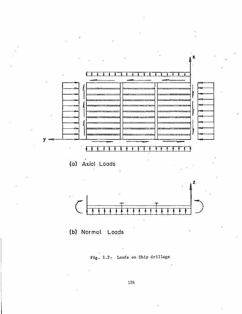
y
x
t t t t t t V t t t • t i ," T T t •- - -j
1 -
1- ....- =
(a) . Axial Loads
z
c ). (b) Norma I Loads
Fig. 1.2: Loads on Ship Grillage
124
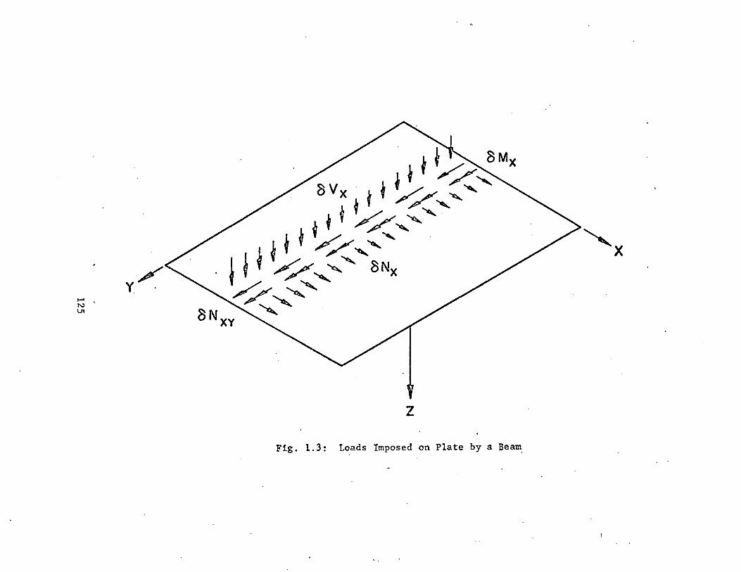
t-'",,'IJ1
Fig. 1. 3:
z
Loads 1m .. posed on PIate by a B.' earn
" X
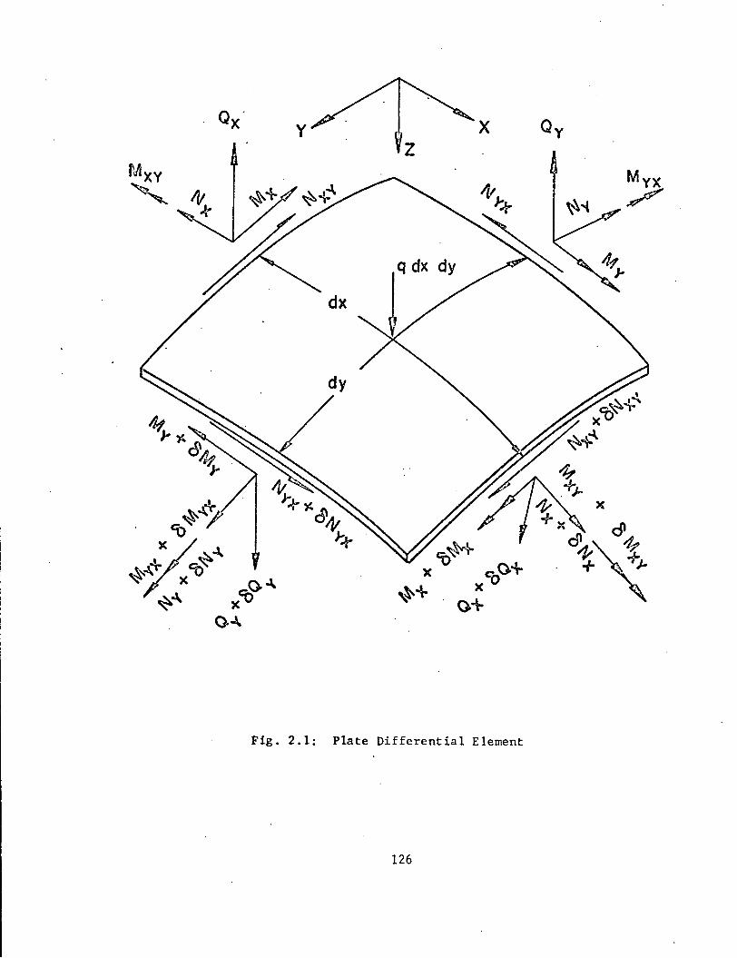
y x Oy
rig. 2.1: Plate Differential Element
126

Case I
~..=-_--j --_......c===::1
Case 2I I~ ~ __--.1-
Case 3
Elastic
.1
Plastic
Case 4 Ca'ses 586
Fig. 2.2: Location of Elastic-Plastic Interfaces
127
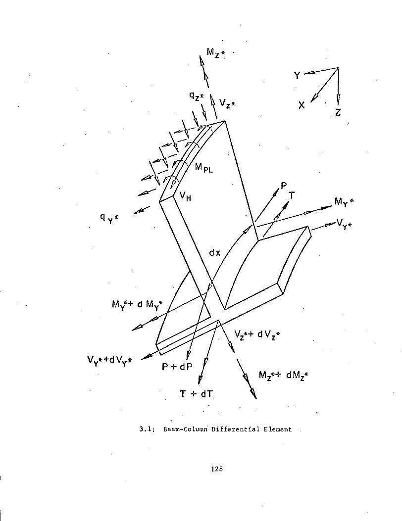
301:
T + dT
. . nOfferential ElementBeam-Column ~
128
y71X z
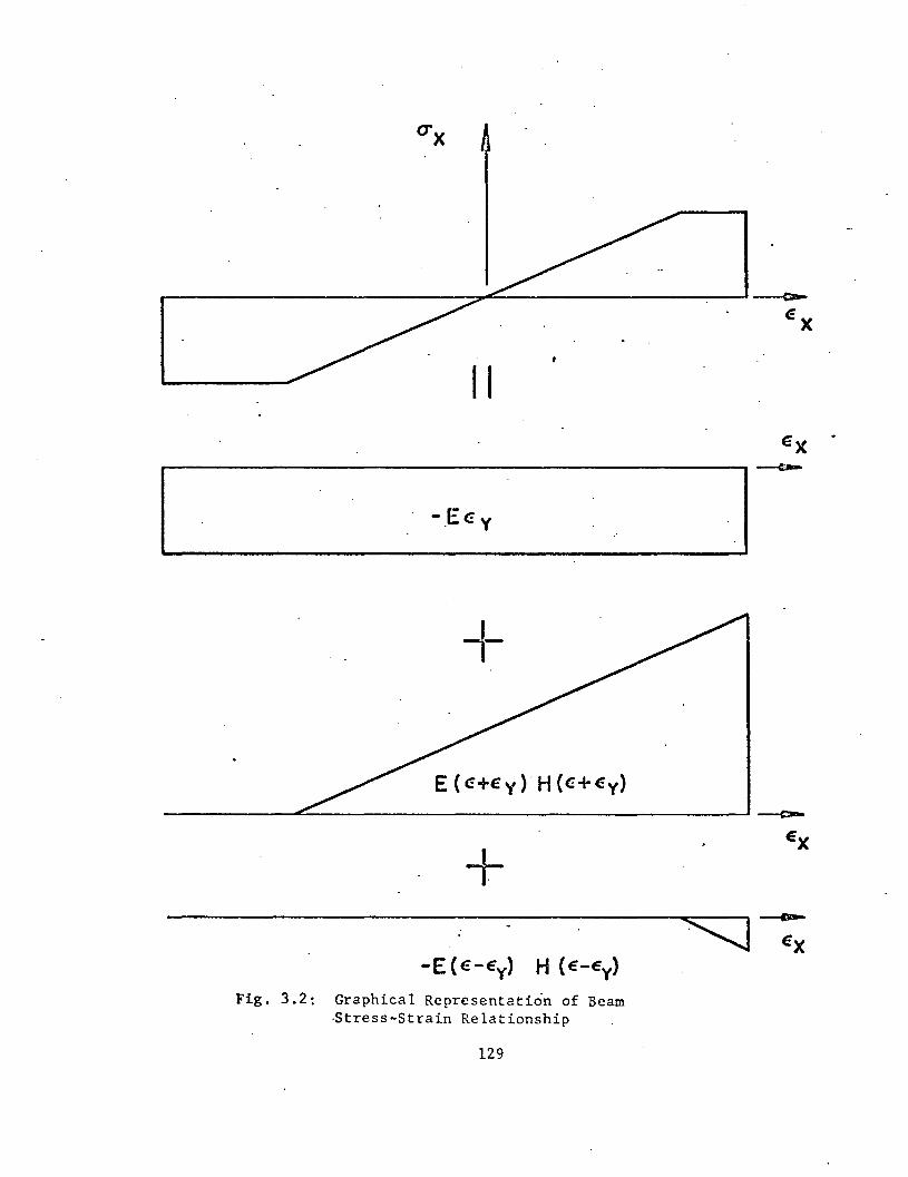
t'>JI-
E x
IIEX
-.E C! y 1--t-
E ( C! +E Y ) .H «(E +E y)
------.L::.--------------------~_e_
+"'l.
Fig. 3.2: Graphical Representation of Beam·Stress-Strain Relationship
129

IIIII'y/
II/
//
/
Fig ~ 3.3: Distribution of Beam Axial Stress
130
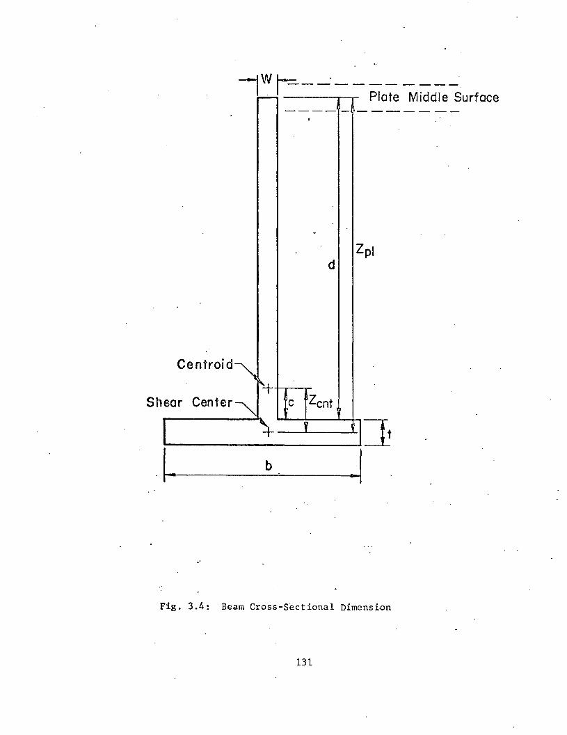
pI
Sh
r-"-
---- -I
-Z
d
Centroid~
~+ear Center~ e Zent
·1
.'
Fig. 3.4: Beam Cross-Sectional Dimension
131

,"
·y --e:I-T-----.,
w
III
c.-_ L.=
(b) Cross Section of a Longitudinal Beam
Fig. 3.5: Displacements of Beam Cross Section
132
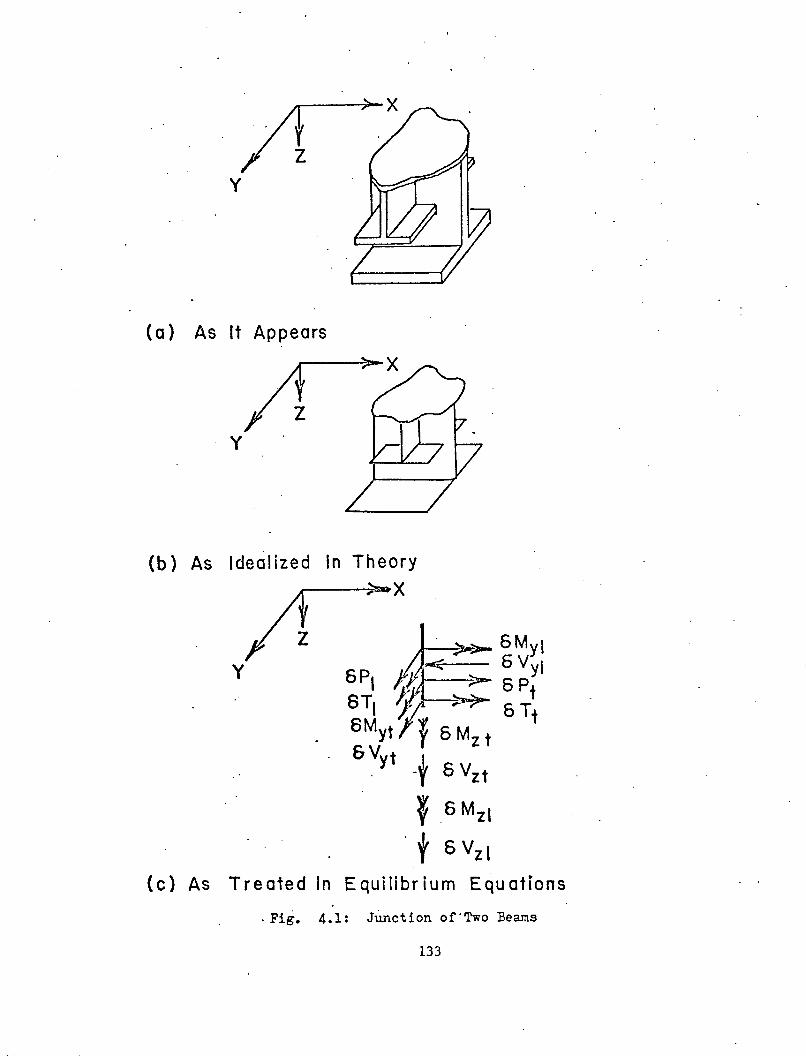
y
(a) As It Appears
y
(b) As Idealized In Theory---~raa-X
y
(c) As Treated In Equilibrium Equations
. Fig. 4.1: JUnction of·Two Beams
133
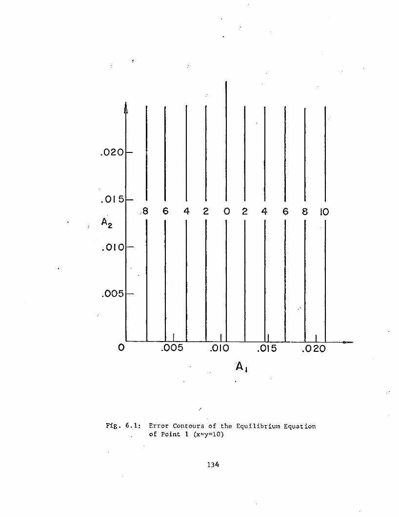
o
"-
to-
:8 6 4 2 0 2 4 6 8 10
f-
I--
I I I I
.020
.015
.010
.005
.005
,"
.010 .015 .020
Fig. 6.1: Error Contours of the Equilibrium Equationof Point 1 (x=y=10)
13"

.00010
-.00005
-.00010
.020
Fig. 6.2: Error Contours of the Equilibrium Equationof Point 2 (x=y=lS)
13S
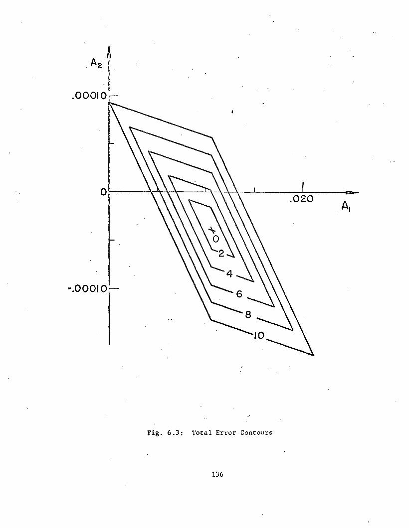
. "
·00010
-.00010
Fig. 6.3: Total Error Contours
136
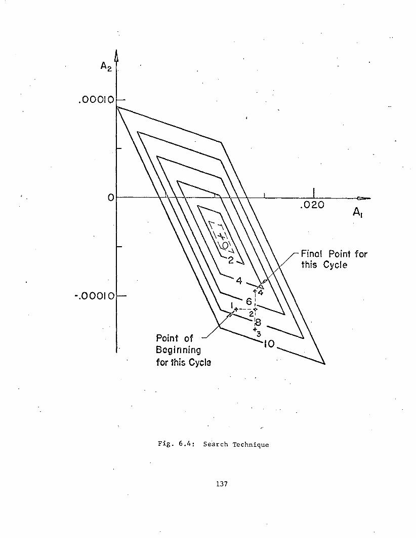
.00010
oL-~1A\--=::~~\-L---.r;0;-t;2()0-~A~I
Final Point forthis Cycle
-.00010
Point ofBoginningfor this Cycle
F · 6 4· Search Technique1.g. "
137

.00010
Ot---~~-T----L~r\---\----L_-_--L_---o--
.020
-.00010 I
Fig; 6.5: Illustration of Valley Point Problem
138
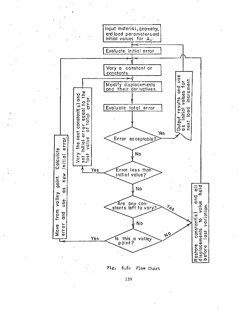
~.
eL
CI> CI>+-
'":J 0.Q +-0 c
U --: ~
CI>c c00.
(/)
>- 0
C1>
CI>0 (/)
> ::J
E-oo c.:: 0
CI>L.
> 00 L.
L.~ C1>
Yes
Yes
Input materia I, geometry,ord load para m'eters ardinit ial va lues for AT
Evaluate initial error
Vary a constant orconstants
Modify displacementsand their derivatives.
Evaluate total error
Fig. 6.6: Flow Chart
139
=-00Ci)
.cucOCl>
:J Co 0
->:;:(/) 0- --+-O~cot- 0o >+-(/)(/)c .... +Oc(/)(.1 CI> 0
E-CI>
Cl>OCl>oo~+.- 0(/) 0._CI>_~ CI>0::-0.0
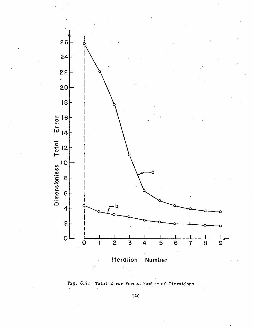
I1
22IIIIIIIIIII
~ 12 Il- I"
010 I
I0Q) -I- 8c:0 I-(/)
Jc:CD 6 IE I.-0
~4
----0--2 III
I I I I I I I 1 1>-0,0 I 2 3 4 5 6 7 8 9
Iteration Number
Fig. 6.7: . Total Error Versus Number of Iterations
140

II
-CO~
. ~ " ~. 2411
= 72.11
~-~ >i--"-=<-=1-r--r
I I, 1'1 II II I ~ II II 1:1 II II II, r: ~ : :1 1III III II II I I}II ~ I I II II" I II I
-----~~----~~----- .'-=---=--=--=- III I --=----- Ttl------=--~ ~-------ll-----~----- ;\
. III I . I ~ I
: II I ·1:' ~11'1 d I1II I 11I 1III I III I1'1 I I III, I I I! !I I ! I
------~----------- ,=-_-_-_-_- I II , __-_-_- I-=-J-_-_-_-_-~~_+_
_____~~----~~----- J
I ~ I II ~ I IIii I II I II I . II I II I II I I II I ~ II I ~ II I I ,I I
" . Fig. 6.8: Grillage Example
141

COLUMN NUMBER
I 1·fF,2~=~3===4:f===5=11'F6===f:7=r-_~2
x
.I ·
3~0::-
· tJ-w:E::£>-en
0:::4
lL.1JJ °co
en~ -:::> xz <t
·~ en-°50:::6 ~
7
__..J.I.-_ • _-,--_ _ __
<t IS AXIS OF SYMMETRYy
--fL-- .
Fig. 6.9: Points of Collocation
142
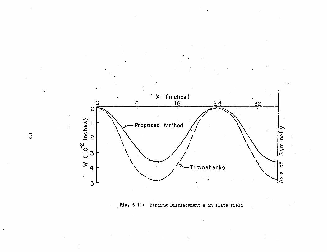
"
I+-o
~....-.(1)
EE~
(j)
en><
. <X:
32x (inches)
8 16oo
-
5
-(J) I'(1)'
J::.o.= 2
C}Jo-3
,Fig. 6.10: Bending Displacement w in Plate Field
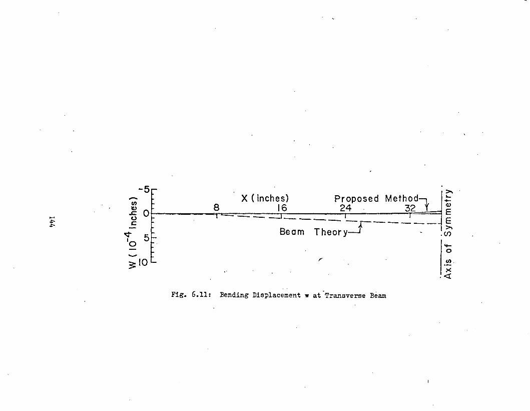
.....o
~
X ( inches) Proposed Method1 .::~ ~=- ;:16:::.- ...:2:;..4..:...-._. 3:::r2~=='==1 E
--- -sea:-Th~y=r-----"~
-5-t/) 8'Q)
0.s:::.~ 0~ &::~
v 5'0
-::=:10
Fig. 6.11: Bending Displacement w at "Transverse Beam

-
- -5 Y ( inch e s)CR
Ct> 16 32 48 >-13 0 ...c: R":-==~Lr=:r===:=I:::::::=:::::::---,---=t-.....~---;:6:r:4~~· Q;
f~ "Proposed Method /" ~~ // ", ~
"A ""'-_/ "'-Beam Theory '- .......1]"<t
Fig. 6.12: Bending Displacement w at Longitudinal Beam
145

c. iL APPENDIXES
146
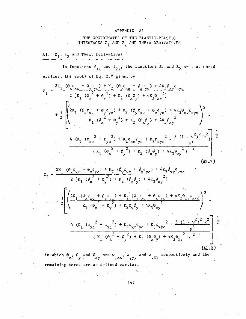
APPENDIX Al
. THE COORDINATES OF THE ELASTIC-PLASTICINTERFACES 21 AND 22 AND THEIR DERIVATIVES
AI. 21
, 22 and Their Derivatives
In functions fli
and f2i
, the functions 21 and 22 are, as noted
earlier, the roots of Eq. 2.8 given by
(0 €x xc
(0 € + 0 € ) + K2 (0 € + 0 € ) + 4K3
0 €x xc y yc y xc x yc xy xyc
2 [Kl
(0 2 + 0 2) + K2
(0 0 ) + 4K3
0 2Jx y x y xy
+ 0 E: ) + K2 (0 € + 0 € ) + 4K30 € )2y yc . y xc x yc xv xyc
(0 2 + 0 2) + (0 0 ) + 4K3
0 2 ' -Kl x· y "K2 x y xy
_ ,})2 k2 1
4 (Kl2 2 2 3 (1 2(€ + € ) + K
2€ € t K3€
E2
)xc yc xc yc xyc
( Kl(0 2 + 0 2) (0 0 ) + 4K3~ 2)
2+ K2x y x y xy
(Al.J.)
(~€ '+0 € ) + K2 (0 € + 0 € ) + 4K30 €x xc yyc y xc x yc xy xyc
2 [K (~2 + 0 ,2) + K2(~0 ) + 4K
3f/J 2J1 x y x y xy
(0 € + ~ € )x xc y yc
(0 2 + 0 2). Kl x y
+ K2 (0y€xc + 0x€y~)
+ K20 f/J + 4K3
0 2x y xy
+ 4K30 € \ 2
xy xyc j
).,
1
4 (Kl (€xc
2 + 2 "2 3 (1 _ })2 k2
2€yc ) + K2€ € + K € .
F2xc yc 3 xyc
(0 2 + 0 2)" (~ ~ ) + 4K f/J2 2
( Kl+ K2 )x y x y " 3 xy
( (Alo2)in which f/J ,0 and f/J are w ,wand w respectively and the
x y xy ,xx ,yy ,xy
remaining terms are as defined earlier.
147
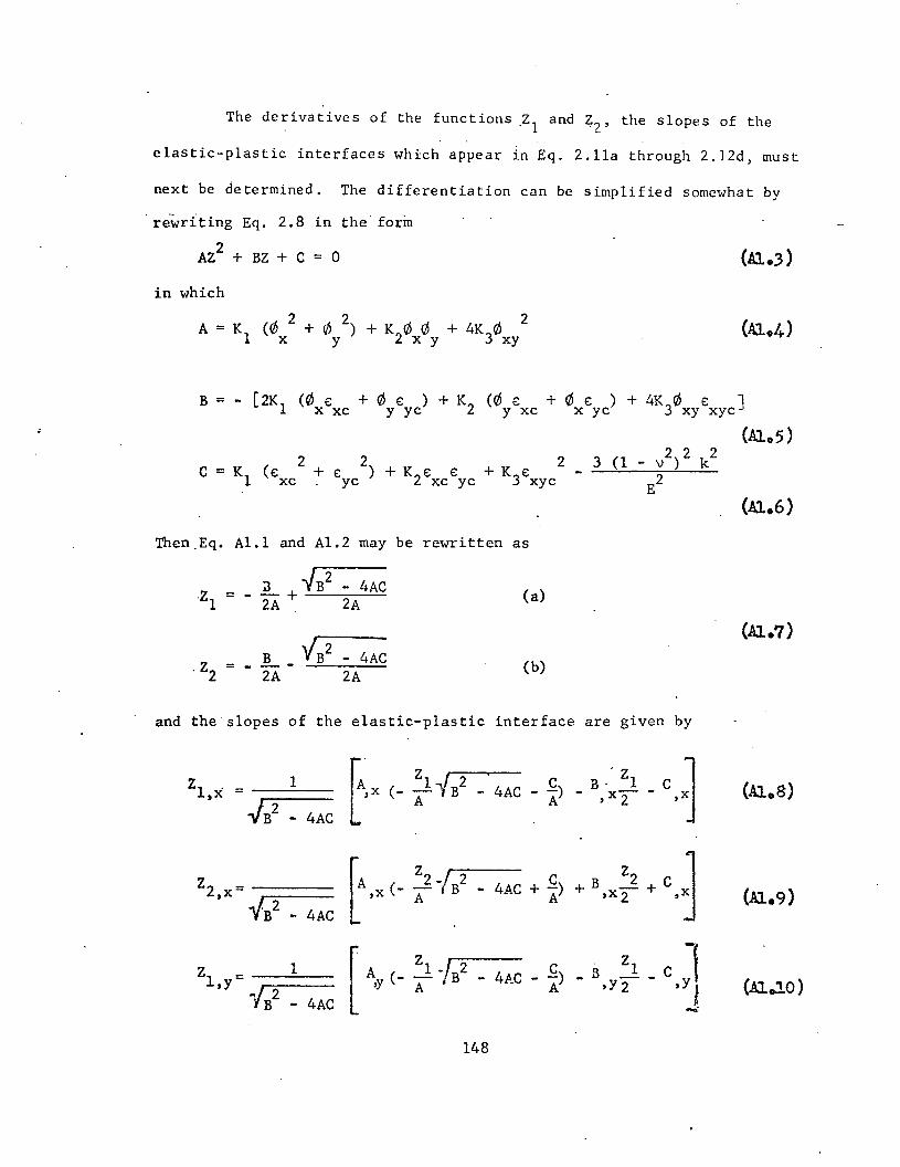
The derivatives of the functions ,Zl and ~2' the slopes of the
elastic-plastic interfaces which appear in Eq. 2.lla through 2.l2d, must
next be determined. The differentiation can be simplified somewhat by
-rewriting Eq. 2.8 in the form
AZ2 + BZ + C = 0
in which
A = Kl
(0 2 + 0 2) + K20 0 + 4K
30 2
x y x y xy
B = - [2K (0 € + 0 € ) + K2 (0 € + 0 € ) + 4K 0 € J1 x xc y yc y xc x yc 3 xy xyc
(Alo5 )
2 t' 2) 2C = K (€ + ~ + K2€ € + K3€1 xc yc xc yc xyc
(Al.6)
Then.Eq. Al.l and Al.2 may be rewritten as
:a -JB2 _ 4AC (a)-Zl = - 2A + 2A
(Al.7 )
. Z2B YB2
- 4AC (b)= - --2A 2A
and the slopes of the elastic-plastic interface are given by
Zl . = 1.x~B2 - 4AC
- 4AC - f)A
'z ~B· 1 C- x- - x
'2 '
Zl = -:::::1==.y .. f 2
YB -
C Zl- 4AC _ -) - B -
A .y 2
(Al.9)
(AlcJ.O)
148

z = 1. [A (_ Z2 -/B2 _ '4AC _. ~) + B Z2 + C j2,y /2 ,Y A. A • ~Y2 '
1: B - 4AC.
(AJ.oll)
Equations A1.8 through AI.II can be placed in a somewhat more convenient
form by taking advantage of the identities
(a)
fB24= - AC
A(b)
(c)
00.13)
(Alo15 )
(Alo16)
In order to express the slopes of the elastic-plastic interfaces
in terms of the curvatures and m~J7surface strains, Eq. AI.13 through
Al.16 may be rewritten employing the expression for A in Eq. Al.4 and
the derivatives of At Bt and C given below in terms of differential
149

functions of the curvatures and mid-surface strains.
A = Kl (2~ ~ + 2~ 0 ) + K2
(0 . 0 + ~ 0 ) + 8K30 0
,x x X,x y Y,x X,x Y x y"x xy XY,x(Al.l?)
A = K (2~ ~ + 20 ~ ) + K (0 0 + 0 0 ) + 8K 0 0,y 1 x x,y y y,y 2 x,y y x y,y 3 xy xy,y
(Al.IS)
B =-t2K (0 8 + 0 8 + 0 8 + 0 8 ) + K (0 8 +,x 1 x,x xc x xc,x y,x yc y yc,x 2 y,x xc
o 8 + 0 8 + 0 e ) + 4K3
(0 8 + 0 8 )]Y XC,X X,X yc x yc,x xy,x xyc xy xyc,x
(Al.19)
B - - [2Kl
(0 8 + o 8 + 0 8 + o 8 ) + K (0 8 +,y x,y xc x xc,y y,y yc y yc,y 2 y,y xc .
o 8 + ~ 8 + ~ e ) + 4K (0 e + 0 e )Jy xc,y x,y yc x yc,y 3 xy,y xyc xy xyc,y
(Al.20)
c = [K (28 8 + 28 8 ) + K (8 8 + 8 8 ),x 1 xc xc,x yc yc,x 2 xc,x yc xc yc,x
+ 2KJG 0xyc.xyc,x
c = [K (28 8 + 28 8 ) + K2
(8 8 + e E: ),y .1 xc xc ,'y yc yc,y XC,y yc xc yc,y+ 2KJo e
(Al.22)xyc xyc,yFor the present, however, this will not be done because of" the obvious
unwieldiness of the resulting expression.
The curvatures of the elastic-plastic interfaces, to be used in
the second derivatives of fli
and f2i
, are determined by differentiating
Eq. Al.13 through Al.16 to obtain
Zl,xx
(Al.23)
150

Z 12 ) [(A 2
2,xx A (2 - (2 1 - 22 ) + A' (2 - 22,x» 2 (A 221 - 2 'x 1,x 2,x ,xx
+ 2 A Z 2 + B 2 + B 2 + C ) J,x 2 2,x ,xx 2 ,x 2,x . ,xx (Al.24)
1 [(A (21
- 2 ) + A '(2 - 2 » 2 +Z =1,yy A (2 - 2
2) ,y 2. 1,y 2,y 1,y
!
(A ,yy2 2 + 2A 2
12 + B 21
+ B 2 + C )J1 ,y l,y ,yy ,y 1,y ,yy
(Al.25)
+ 2A 22 Z + B Z2 + B 2 + C )J,y 2,y ',yy ,y 2,y ,yy (Al
o26)
Z2,yy1
- - -A--:-(2-1"'::-"--2-
2"-) [(A,y (2 1 - 22 ) + A (2 1 ,y
(A ,yy Z/
22 » 2 -,y 2,y
22 » 2, +,y +,x
2(A Zl + 2A 21 2 + B 21 + B 21 + C )J
,xy ,x 1,y ,xy ,x,y ,xy (Al.27)
12 - - -----2,xy A (2 1 - 22)
(A 2 2 + 2A 22
2 + B 2 + B 2 + C )],xy 2 ,x 2,y ,xy 2 ,x 2,y ,xy (Al.28)
In order to express Eq. Al.22 through Al.27 as differential functions'
of the plate curvatures and mid-surface strains, the previously defined
functions 21, 22 , 21•x ' 21 ' 22 ' 22 ' A, B, A, A , Band C must• ,y ,x,y ,x x ,x
be used in conjunction with the following expressions for the second
derivatives of A, Band C.
A = 2K1 (0 0 + (0 )2 + 0 0 + (0y ,x)2) + K2 (0x ,xx0y,xx x,xx x x,x y,xx y
+ 2~ ~ + ~ ~) + 8K; (~ ~ + (~ )2)PX,XPy,x Py,xxPx P P PXY.xx xy XY,x
151
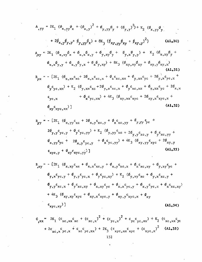
A = 2K1 (0 0 +. (0 )2 + 0 0 + (0 )~ + K2
(0 0·,yy x,yy x x,y y,yy y y,y. x,yy y_
(Al.30)
A 2K (0 0 + 0 0 + 0 0 + 0 0 ) + K (0 0 +;Xy 1 x, xy x x, x x, y y ,xy y y ,x y, y 2 x ,xy y
o 0 + 0 0 + 0 0 ) + 8K (0 0 + 0 0 )X,x y,y x,y y,x x y,xy 3 xy,xy xy xy,y xy,x(Al o31)
B = - [2K (0 8 + 20 8 + 0 8 + 0 8 + 20 '8 +~x 1 x,XX xc X,x xC,x x xC,xx y,xx yc y,x yC,x
o 8 ) + K2
(0 8 -+ 20 8 + 0 8 + 0 8 + 20y yc,xx y,xx xc y,x xC,x y xC,xx ~,xx yc X,x
8yC,x
o 8 )]xy.xyc,xx
+ 0 e: ) + 4K (0 8 + 20 e: +x yC,xx 3 xy,xx xyc xy,x xyc,x
(Al.32)
B = - [2K1
(0 8 + 20 8 + 0 e: + 0 €;/y x,yy xc x,y xC,y x xc,yy y,yy yc+
o e: +x,yy yc
20 e: + 0 8 ) + K (0 8y,y yC,y Y yC,yy 2 y,yy xc + 20 8 + 0 e: +y,y xC,y y xC,yy
20 € + 0 e: ) + 4K (0 e: + 20x,Y yc,y x yC,yy 3 xy,yy xyc xy,y
e: + 0 e .J]xyc,y xy xyC,yy(Al.33)
B = - [2K (0 8 + 0 8 + 0 8 + 0 e: + 0 8 +,xy . 1 x, xy xc x, x xc, y x, y xc, x x xc, xy y, xy yc
o 8 + 0 8 + 0 e: ) + K (0 e: + 0 e: +y,x yc,y y,y yc,x y yC,xy 2 y,xy xc y,x xc,y
0 8 + o 8 + 0 e: + 0 e: + 0 e: + o 8 )y,y xc,X y xc,xy x,xy yc X,x yc,y x,y yC,x x xC,xy
+ 4K (0 8 + 0 8 + 0 8 + ~3 xy,xy xyc xy,x xyc,y xy,y xyc,x xy
E:xyc,xy)] (Al.34 )
c = 2K1
(8 e: + (8 )2 + (8 )2 + e: e: ) + K (e: e:~Xx XC, xx xc xc , x yc ,X yc yc, xx 2 xc ,XX yc
+ 2E: . 8 + 8 e: ) + 2K (e: e: + (e: )2 (Al.3S)xc,X yc,x xc yc,xx 3 xyc,xx xyc xyc,x
152

c = 2K(£ £ + (£ )2 + (£ )2 + £ £ ) + K (e £,yy 1· xc,YY xc xC,Y yc,Y yc yc,yy 2 _xc,yy yc.
2+2£ £ + 8 8 ) + 2K (£ £ + (8 )xc,y yc,y xc yc,yy 3 xyc,yy xyc . xyc,y (Al.36)
C = 2K (£ 8 + 8 8 . + 8 8 + 8 8 ) + K .,xy 1 xY,xy xc xc,x xy,y yC,x yc,y yc yc,yy 2
(8 8 + 8 8 . + 8 8 + 8 8 ) + 2K (8xC,xy yc xc,x yc,y XC,y yC,x xc yc,yy 3 xyc,xy
8 + 8 8 )xyc xyc,x xyc,y (Al. '37)
In order to express the differential ~quations of elastic-plastic
plates in terms of the .plate displacements, the strain and curvatures
appearing in Eq. Al.l through Al.37 must be expressed as differential
functions of the plate deformations. This is "accomplished by means of
the s.train displacement re lationships shmvn in Eq. 2.4 and the following
derivatives of the generalized strains.
o =wx,X ,xxx
o = WX,xx ,xxxx
0=0 = wx,y xy,x ,xxy
(A1038)
(Al.39)
(Al.40)
o = 0x,yy y,xx
o = wx,xy ,xxxy
o = wxy,xy ,xxyy (Al.41)
(Al.42)
0=0 = wy,x xy,y ,yyx
0=0 = 0 = wy,xx x,yy xy,xy ,xxyy
I
153
(Al.43)
(Al.44)
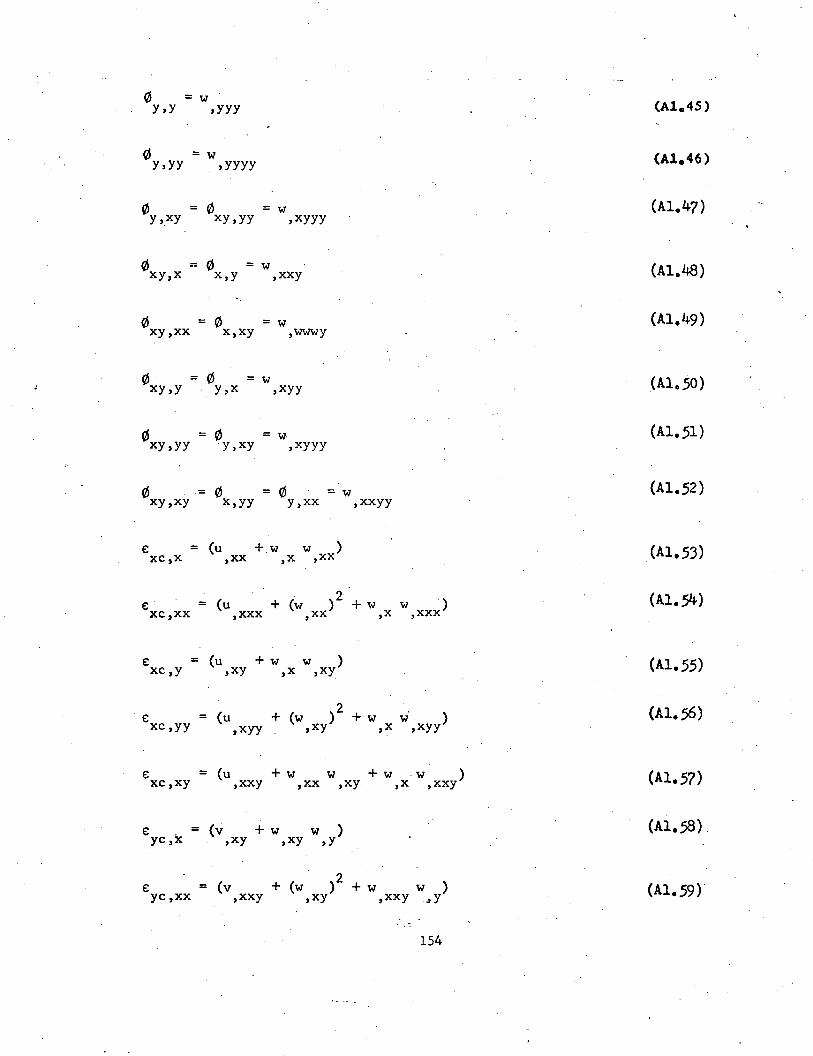
0 = wy,y ,yyy
0 = wy,yy ,yyyy
0 = 0 = wy,xy xy,yy ,xyyy
0 = 0 = wxy,x x,y ,xxy
0 = 0 = wxy,xx x,xy ,wwwy
0 = 0 = wxy,y y,x ,xyy
0 = 0 = w·xy,yy ·y,xy ,xyyy
0- 0 = 0 = wxy,xy x,yy y,xx ,xxyy
€ = (u +.w w )xc,x ,xx ,x ,xx
€ . - (u xxx + (w xx)2 + w w xxx)xc ,xx, , ,x,
€ = (u ,xy + w w )xc,y ,x ,xy
(u2
W,xyy)€ = + (w,xy) +wxc,yy ,xyy ,x
€ = (u ,xxy +w w +w . w )xc,xy ,xx ,xy ,x ,xxy
€ = (v + w w)yc,x ,xy ,xy ,Y
(v,xxy + (w2
w )€ = ,xy) +wyc,xx ,xxy 3Y
154
(Al.50)
(Al.5l)
(Al.52)
(AI.53)
(Al.54)
(Al.55)
(Al.56)
(AI.58) .

e: (v +w W )yc,y ,yy ,yy ,y
e: = (v + (w )2 + w w )yC,yy ,yyy ,yy ,yyy ,y
e: = (v +w w +w w )yC,xy ,xyy ,yy ,xy ,xyy ,y .
(Al.60)
(Al.61)
(Al.62)
e:xyc,x
(Al.6J)
e: = (v + u + 2w w +w -w +w w )xyc,xx ,xxx ,xxy ,xx ,xy ;xxx ,y ,x ,xxy (Al.64)
e: = (v + u- +w w +w W,yy) (Al.6S)xyc,y ,xy ,yy ,xy ,y ,x
e:xyc;yy= (v + u + 2w w + w w + w w )
,xyy , yyy ,xy, yy ,xyy, y , x ,yyy (Al.66)
e:xyc,xy= (v + u + (w )2 + w
,xxy ,xyy ,xy ,xxyw
,Y+w
,xxw
,yy+w w
,x ,xyy(Al.67)
To evaluate the expressions for Zl and Z2 and their derivatives,
the values for the generalized strains and their- derivatives are first
introduced into the expressions for A, Band C and their derivatives.
These values are introduced in turn in the expressions for Zl and Z2
and their derivatives to obtain their numerical values. These values,
in turn, are introduced into the expression for fli
, f2i
and their
derivatives given in Appendix A2.
155

A2. THE FUNCTIONS OF THE LOCATIONS
OF ELASTIC~PLASTIC INTERFACES
The functions f1i (Zl' Z2' h),and f 2i (Zl' 'Z2' h) are as
tabulated belowo
~ f1i (Zl' Z2' h) f 2i (Zl' Z2' h)case
1 Z 2 _ Z 2 - h (Zl + Z2) Z 3 3h2(Z - Z ) - Z 3
1 2 1 - -4- 1 2 2
Z 2 h2Z 3 _
3h2Z h32 - hZ + 1
1 1 4 1 4 -4
2 h2_ Z 3 +
3h2Z .h3
3 2- (Z2 + hZ2 + 4) 2 4 4
4 0 h3- 2
.5 - 2hZ 0I 1
6 - 2hZ 0.' 2
-
156

'"The first partial derivatives of fli
and f2i
~nth respect to x are:
function f . (Zl' Z2' h) (Z , h)f 2i ,x Z ,i 1J.,X 1 2
2(Z Zl - Z Z2 ) 3(Z12Z 2- Z2 Z )
1 1 ,x 2 ,x 2 l,x 2,x- h(Zl + Z ) - 2h.... (Z - Z )
,x 2,x 4 l,x 2,x
2 22 2Zl
Z - hZ 3Z Z - JlL Zl,x l,x 1 l,x 4 l,x
3 - 2Z Z -2 2
hZ2 - 3Z2 Z2 + 2h- Z22 2,x ,x ,x 4 -,x
4 0 0
5 - 2hZ 0l,x
6 - 2hZ 02,x
* To obtain expressions for the first derivatives with respect to y,
x is replaced by y in the above tabulation.
157

The second partial derivatives of fli
are not required. The second
partial derivatives of f2i
are:
function *f (Zl' Z , h)i 2i,xx 2
I 2 2 . 2 23(ZI Zl - Z2 Z2 + 2ZI (Z ) - 2Z2(Z2 )),xx ,xx l,x ,x
- 3U2
(Zl - Z ),xx _,2,xx
22 2 2
3Z1 Zl + 6z (Z ) - 2h- Z,xx I l,x 4 l,xx
2 .223 -3Z2 Z2 - 6Z2(Z2 ) + 2h- Z2,xx ,x 4 ,xx
4,5,6 0
* To obtain f2
, ,x is replaced by y in the above tabulation.. J.,YY
function
i
I
2
3
4,5,6
£2' (Zl' Z , h)J.,xy 2
3( Z12Z1 - Z 2Z ) + 6(ZI Z ~Z - Z2Z~xZ2 ),xy 2 2,xy l,x ,l,y ',y
- 3h2
(Zl - Z2 )4 ,xy ,xy
2 23Z
1 Zl + 6Z1Z1 Z . - 2h: Zl,xy . ,x l,y 4 ,xy
o
158

APPENDIX A. 3 BEAM GENERALIZED STRESSES MID THEIR DERIVATIvES
The integrals to be evaluated in Eqs. (3.7), (3.8), and (3.9)
are of the form:
Int. (g (y,z» dy dz (A3.l)
in which Yl , Y2
, Zl' and 22
, the limits of integration, represent edges
of the cross section, f (y,z) is a force or moment per unit area, and
g (y,z)is the difference between the yield strain and the strain at a
point, and H (g (y,z» is a Heaviside unit step function with g (y,z)
as an argument. Integration of these functions is accomplished as
follows. First, the function is integrated by parts in y to obtain:
J22 [ \ Y2 JZ2Int. = . F(y,z) H (g (y,z» Y - F (y,z)2
1. 1 2
1.
5 (g (y,z» dyJdZ
(AJ.2)
in which the function F (~,z) is the antiderivative in y of f (y,z)
and 5 (g (x,y» is the Dirac delta function with g (x,y) a~ an argument.
The product F (y,z) H (g (y,z» \:2 is a function of z alone1
after the limits of integration are introduced to obtain:
(A3.3)
Integr~tion of a typical product of this type by parts in z results in
expressions of the form:
159

, 1Zdz = F (Yl'Z)' H (g (Yl ,z) /
1
(A3.4)
in which F (Yl,z) is F (Yl,z) integrated in z. In this instance, both
the Heaviside step function and the Dirac delta function are functions
of Z alone.
I Z2 -.The integrals of the form F (Yl,z) ,0 (g (Y
l,z» dz assume
, Zlvalues of Sign 0 i (Yl,ZEPI) in which ZEPI is the intercept of one of
the lines g (y,z) = 0 and the line y = Yl
(a zero of g (Y~,z» if this
point is within the portion of the cross sec tion of interest. Otherwise
they ~re zero. The term Sign 0 is positive or negative unity ~ccording
to the sign of the delta function.
The final type of integral to be considered is the last part
. of Eq. (A3.2):
f. Z2. 'f Y2 F (y,z) 0 (g (y,x» dy dzZl Yl
This is a line integral defined on the line for which g (y,z) :;; O.
To accomplish the integration, y in F (y,z) is defined as a function of
z by means of the relationship g (y,z) = 0 and then F (z) is integrated
in z from the minimum to maximum z value of the appropriate line
g (y,z) = 0 to obtain i (z) I:m~x.if g (y,y) = 0 within the limits andml.n
otherwise zero.
The integral given by Eq. (A3.l) in the notation used above can
160

be written as follows:
- F (Yl ,Z2) + F (yl,Zl) + Sign (6 (Yl,Z» F (Yl,ZEPI)
F (z) \ :m~x (A). 5)nan
Writing the integrals defining the generalized stresses can be
greatly simplified by means of an abbreviated notation. The integral
defining M can be written in terms of the following functions, with AUXlz·
a function of the .form given earlier as F (y. ,z.) H (g (Y.,z.», AUX2 of~ ~ ~ ~
- = \Zmax .the form Sign (6) F (Yi,zEPI) and AUX3 of the form F (z) Z ... m~n
W2c W
AUXl CW,c,e:Y)=-S-(e: --v -,sw +e:)H(e: -~v - cWb +e:)o 3 b,xx 2 b ,x x Y 0 ~ b, xx ,x x y
'..
w· 2 2AUX2 (Zf' W, c, c-d) =lwb'XXI~6 [Zf
b,xx+ ~ Z Jwb,xx 3 f vb,xx
(AJ.. 6)
(A3.7)
(A3.8)
M = - E [AUXl CW, c, e: ) - AUXl (\'1, c.-d, E: ) + AUX2 (Zf' W, c, c-d)z y. y
- AUXl (-\-1, c,. E:y) + AUXl (-W, c-d, e: y) - AUX2 (ZG' -W, c, c-d)
161
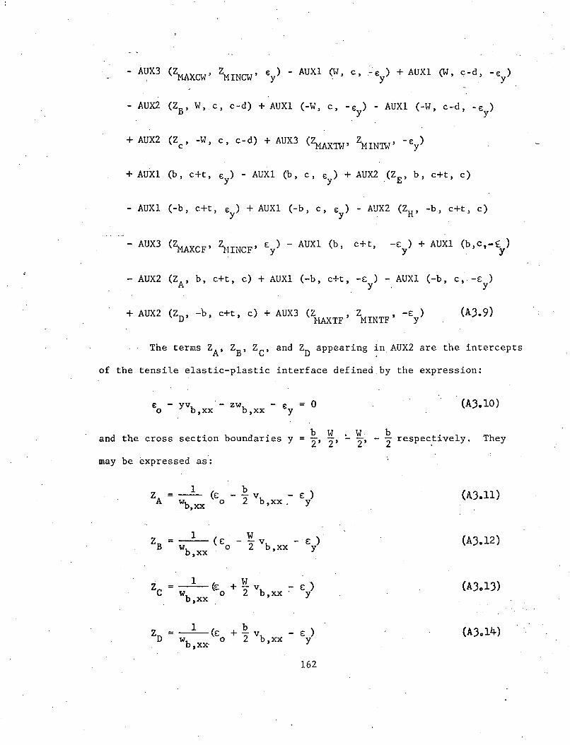
- AUX2 (ZB' W, c, c-d) + AUXl (-W, C, -€y) - AUXl (-W, c-d, -€y)
+ AUX2 (Zc' -W, c, c-d) + AUX3 (~AXTW' ZMINTW' -€y)
+ AUXl (b, c+t, € ) - AUXl (b, c, € ) + AUX2 (ZE' b, c+t, c)'y y,
- AUXl (-b, c+t, €y) + AUXl (-b, c, €y) - AUX2 (ZH' -b, c+t, c)
- AUX3 (11AXCF' ;lINCF' E.y) - AUXl (h, c+t, -£ ) + AUXl (b,C,-f )y . y
- AUX2 (ZA' b, c+t, c) + AUXl (-b, c+t, -£ ) - AUXl (-b, c,-£ )Y Y
+ AUX2 (ZD' -b, c+t, c) + AUX3 (Z , Z , -£ )HAXTF MINTF Y
The terms ZA' ZB' ZC' and Zn appearing in AUX2 are the intercepts
of the tensile elastic-plastic interface defined by the expression:
e - yv - zw - e = 0o b,xx b,xx Y(A3.10)
dh 'b d' bW,W b 'Ian t e cross sec t10n oun ar1es y = 2' 2' - 2' - 2 respec,t1ve y.
may be ~xpressed as:
They
ZA1 (£ b £ )=-- - - v -
wb xx 0 2 b ,xx. y,
ZB1 (£ W £ )= --v
W 0 2 b,xx yb,xx
Zc1 (£ W £)= +-v
W 0 2 b,xx yb,xx
Zn1 (£ b £ )= +-v -
wb xX' 0 2 b,xx y,162
(1\3.11)
(A3.12)
(A3.13)
(A3.14)
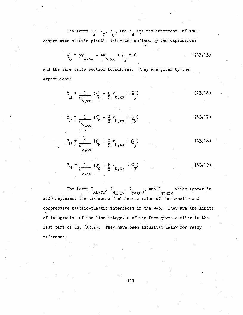
The terms Z , Z , Z t and Z a~e the intercepts of theE F G . H
compressive elastic-plastic interface defined by the expression:
( = YV - zw + t. = 0 (A).IS)o b,xx. b,xx Y
and the same cross section boundaries. They are given by the
expressions:
Z = I (£ - b v + ~ )E w 0 2 b,xx y
b,xx
Z = I (f - w v + t )F ·w 0 2- b,xx y
b,n
ZG = I (£ +Wv + E )w 0 2' b,xx ybin
ZH = I (€ + b v + £- )w o 2 b,xx Ybin
(A). IS)
The termsZ , Z , Z t and Z which appear in~~XTW MINTW MAXCW MINCW
AUX) represent the maximum and minimum z value of the tensile and
compressive elastic-plastic interfaces in the web. They are the limits
of integration of the line integrals of the form given earlier in the
last part of Eq. (A).2). They have been tabulated below for ready
reference.
163

ZB < (c-d) c-d ~ ZB .~ c ZB > c
~TW ~lINl'i-J ~lAXTW ~INTH ~lAXTi-l ~INTW
" /"0I0'-'
ZB c-d c-d
~·c
VIU
N
0 for ZB > ZcVINU
Zc c-d ZB Zc c ZVI for ZB < Zc
c""0
IZc ZB0
'-'
U ~K1\ c c-d c ZBU /N
Extrema for Tensile Elastic-Plastic Interface in Web
ZF < (c-d) c-d < Z < c· c < ZF- F-
~MAXCH Zl-iINCH Z ZHINCI-l ZMAXCH Zt-lINCHMAXCH
,....,
~V"0I0
ZF c-d c-d'-'
/ ~c
vc.!>
N0
vi Z > ZGFc.!> ZF ZGN
ZG c-d c ZGvi ZF < ZG"0I
Zr, Z",0
0
>/." c c-d c ZF
~c.!>N
Extrema for Compressive Elastic-Plastic Interface in. Web
164
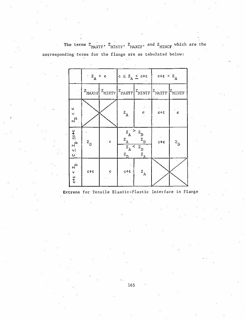
The terms Z~~~TF' ZMINTF' Z~~CF' and ZMINCF which are the
corresponding terms for the flange are as tabulated below:
ZA < c c ~ ZA2. c+t c+t < ZA
ZMAXTF Z~IINTF Z~fAXTF Z~IINTF Zl-fAXTF ZHINTF
0 ~
<v
1/ZA c c+t c
QN
.j..l
ZA > Zn+~I ZA Zn
Q Zn c c+t ZnN
ZA < Znviu· Zn ZA
Q ~RN
v c+t c c+t ZA
/.j..l
+0·
Extrema for Tensile Elastic-Plastic Interface in Flange
165
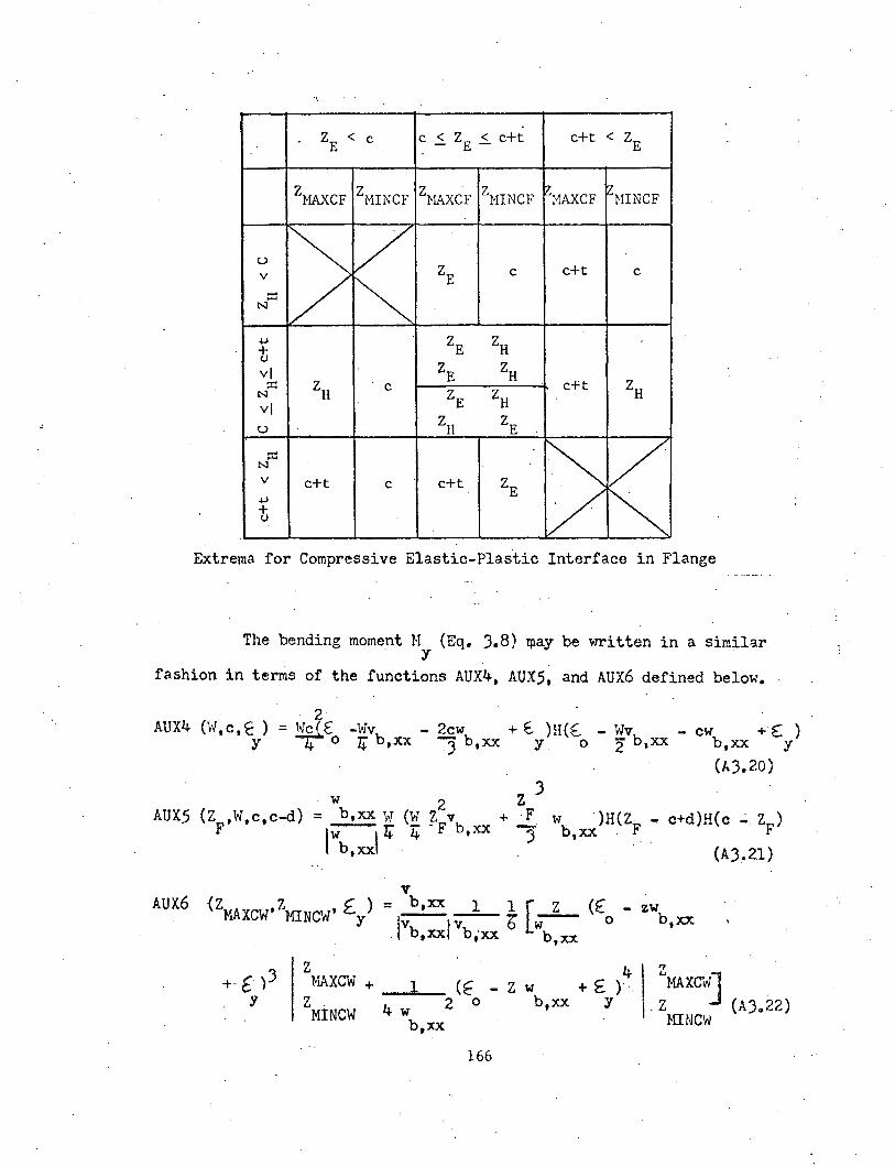
-,
Z < c c < Z < c+t c+t < ZE - E- E
ZMAXCF ZMINCF ZI-lAXCF ZI--IINCFf7 17Il-MAXCF I6HINCF
u
~V ZE c+tc cv
~::r:N
+J ZE ZHtvi ZE ZH
c+t ZH::r: ZH cZHN ZE
vi
u ZH ZE
::r:
~KN
v C+t c C+t ZE+J 1/+0
Extrema for Compressive Elastic-Plastic Interface in Flange
The bending momentM (Eq. 3.8) ~ay be written in a simi13r- y
fashion in terms of the functions AUX4, AUX5, and Aux6 defined below.
2AUX4 (\;T,c,~ ) = h"fl(f -'v-!v - 2cw + E. )H«( - Wv - - e\~ +£ )
y 0 4 b,xx J b,xx Y 0 2' b,xx b,xx Y(A3.20)
AUX5 (Z ,W.e.e-d)F
-w= b,xx \{
IWb ,xx\4
2 Z J(w z v +F w)H(Z --c+d)H(c ~_ Z )- - F b xx -- b~xx _ F F4 3 __
(AJ..21)
v _= b,xx 1 1 [Z (E - zw
Iv Iv 6':;;-- 0 b,xx- b,xxi b,-xx b,xx
Z JMAXC'"w
- Z (A).22)MINCW
4- Z w + £ )'"
b,xx Y(E
2 01
4wb,xx
ZlI!AXCW +
--""'--Z MINCW
166
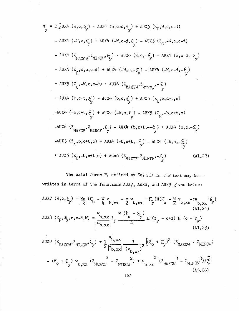
M = F. fAUX4 (itJ,c,£ ) - AUX4 (H,c-d,~) + AUX5 (ZF"H,C,c-d)y '- y y
- AUX4 (-~ltC, ~ ) + AUX4 (-vl,c-d,E) - AUX5 (ZG,-W,c,C-d)Y y
- Aux6 (Z ,2 ,S) - AUX4 (1tI,c,-f ) + AUX1+ C,.J,c-d,-f )YillXCW MINCW y Y Y
- .4.UX5 (Z ,It/,c,c-d) + AUX4 (_i.j,c,-E) - AUX4 (-\<l,c-d,-£ )B y y
+ AUX5 (Z ,-H,c,c-d) + Aux6 (z < ,Z ,- f)C Jvf.AXTW MINT:-l y
+ AUX4 (b,c+t,f) -AUX4 (b,e,f.-) + AUX5 (Z ,b,c+t,c)y EY
-AUX4 (-b,c+t, E) + AUX4 (-b,c,E) - AUX5 (Z ,-b,c+t,c)y y II
-Aux6 (z ,Z ,l: ) - AUX4 (b,c+t,-'--t) + AUx4 (b,c,-£ )li~XCF MINCF y y y
-AUX5 (Z ,b,c+t,c) + AUx4 (-b,c+t,-£) - AUX4 (-b,c,-£,.)A y Y
+ AUX5 (Zn,-b,C+t,c) + Aux6 (ZMAXTF,ZMINTF'-~) (Al.23)
The axial force P, defined by Eq. :3 :'7, ,"in the' text may:' be:,'
written in terms of the functions AUX7, AUX8, and AUX9 given below:
AUX7 (H,c,E.) = We (€ _."'; v - C W + £, )H(f - H v -cw +f;y .2 0 4' b,xx 2' b,xx y 0 '2 b,xx b,xx S
(Al.24)
AUX8 (~,~,c,C-d,W)w W (f - E )
= b,xx Z 'c Y.H
I''''b,xxI F 4(Z - c+d) H (c - z )
F F
(.11025)
v.AUX9 (Z Z r ) = 1 b, xx
J.1AXC'Vi' NINC'tJ'1r'2\Vb ,xxl
2- (£ + £. ) w (z
o y b, xx H.lI.XCvJ
167(A).26)

+ AUX8 (ZF' -€y' c, c-d, W) - AUX7(-W, c, E: ) + AUX7 (-W, c-d, .e )y ',' y
+ Aux8 (Z ,-£ ,c,c-d,W) + AUX9 '(ZMAXCW'Z '£-) - AUX? (W,c,- EJG y , , MINCW Y Y
+ AUX7 (\oJ, c-d, -E:y) - AUX8 (ZB' E:y ' c, c-d, W) + AUX7 (-W, C, -E:y)
- AUX? (-\.[, c-d , - E.) - AUX8 (ZC' f: , c,c-d,W) - AUX9 (ZMAXTW' Zl'IINT'I'l' - ~)y y.
+ AUX7 (b, c+t, E:y) - AUX7 (b, q E:y)+ AUX8 (ZE' -E:y ' c+t, C, b)
- AUX7 (-b, c+t, E:y) + AUX7 (-b, .c,' E:y> + AUX8 (ZH' -E:y ' c+t, C, b)
+ AUX9 (~AXCF' ZMINCF' E:y) - AUX7 (b, c+t, -E:y) + AUX7 (b, c, - E: )Y ,
- AUX8 (ZA' E:y ' c+t, c, b) + AUX7 (-b, c+t, -E:y) - AUX7 (-b, c, -E: )Y
- AUX8 (ZD" E: y ' c+t, c, b) - AUX9 (~AXTF' ~INTF' E:y)]
The first derivative of M may be written in terms of thez
first derivatives of AUXl, AUX2, and AUXJ given below:
W2
cDAUXl fT.T, C, E: ) = -- (E:, , \" 'y 8 o,x
W-v3 b,xxxc- w )2 b,xxx
WH (eo - -2 Vb - cW b + E:y ),xx ,xx
W2 W+ __c (E: - - V - ~ W + E: ) 0 (E: W - cw + e )~ 0 3 b,xx 2 b,xx y 0 - 2 vb,xx b,xx y
(AJ o 28)168
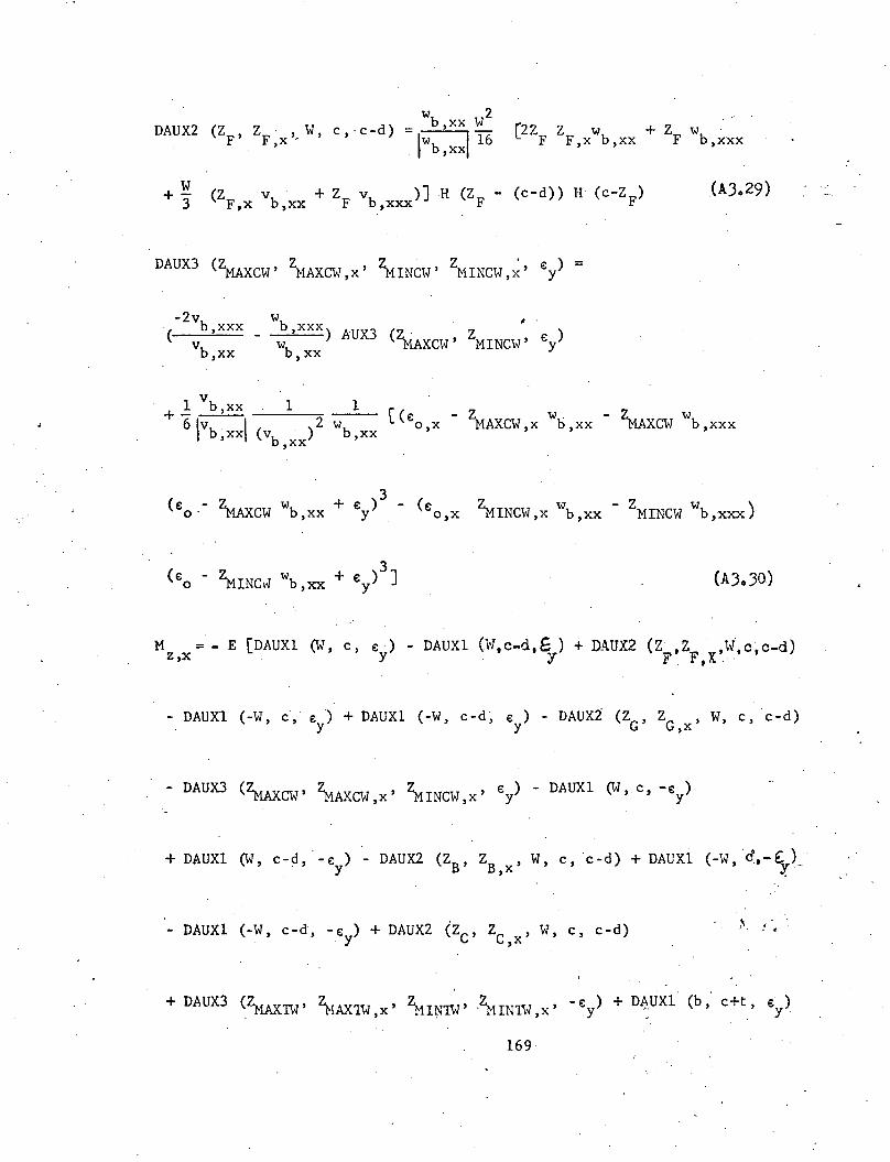
W 2DAUX2 (Z Z W c,.c-d) - b,xx W
F' F~x" , -IWb,xxITI(n Z W + ZF W .
F F,x b,xx b,xxx
DAUX3 (~XCW' ZMAXCH ,x' ~INCH'Z • E: ) =MINCH,x' Y
-2v W #( b,xxx b,xxx) AUX3 (~AXC\o1 ' ZMINCW' E:y )
V Wb,xx b,xx
v+ 1: b ,xx 1
6\v I 2b ,xx (vb . ),xx
1W [(E:o,x - ZMAXCW,x wb,xx - ~XCW wb,xxx
b,xx
(eo .- Z ·XCT.T wb,xx + ey )3 - (eo,x Z W - Z W )-xA V'I ~ INCH, x b ,xx MINCH b ,xxx
( Z W + ~ )3 J ( )eo - ~INCw b ,xx "'y A3030
M = - E [DAUXl (W, c, e) - DAUX1 (W.c-d.G) + DAUX2 (2.Z .•\{.c~c-d)z ,x y. Y F. F. X ...
- DAUXI (-W, c, €y) + DAUX1 (-H, c-d~ €y) - DAUX2 (ZG' ZG,x' W, c,c-d)
- DAUX3 (~CH' ~AXCW,x' ~INCW,x' €y) - DAUX1 (W, C, -€y)
+ DAUX1 (W, c-d,-E:y
) - DAUX2 (ZB' ZB,X' W, c,c-d) + DAUXl (-\01, .~.-£~}
DAUX1 (-W, c-d, -€y) + DAUX2 (ZC' Zc,x' W, c, c-d)
+ DAUX3 (~TW' ~lAX1W,x' ~IN1W' '~IN1io1,x' -ey ) +D~UX1 (b,' c+t, €y)
169
-DAUX1 (b, c, €y) + DAUX2 (ZE' ZE,x' b, c+t, c) - DAUX1 (-b, c+t, €y)
+ DAUX1 c (-b, c, €y) - DAUX2 (ZH' ZH,x' -b, c+t, c)
- DAUX3 (~1AXCF' ZMAXCF,x' ~INCF' ~INCF,x' €y) - DAUX1~(b, c+t, -€y)
+ DAUXl (b, C, -'€y) - DAUX2 (ZA' ZA,x' b, c+t, c) + DAUX1 (-b,c+t,-fy.)
- DAUX1 (-b, C, ~€y) + DAUX2 (ZD' ZD,x' -b, c+t, c) +
+ DAUX3 (~AXTF' Zt-lAXTF,x' ZMINTF' ZMINTF,X' -€y) (AJ.Jl)
The expression for M may be written using the followingy,x
definitions of the derivatives of AUX4, AUXS, and AUX6:
Wc2
W 2cDAUX4 (W, c, €y) = -4 [(€ - -4 vb - -3 wb )o,x ,xxx ,xxx
W& (€o - -2 vb - cWb + €y)J,xx ,xx
DAUX5 (ZF' ZF,x' w, c, c-d) =
(AJ.J2)
3 .wb W W' . W 2 Z 2 ZF,xx _ [_ Z ~ + Z + Z + 1~ - v. F W":b -3 \Vb xxx w\wb ,xxI 4 .2 F ;X o,xx 4 F b,xxx F,x,xx , .
170
v vDAUX6 (Z Z Z Z ) - b ,xx 1 [ b ,.xxx
HAXCW' HAXCW ,x' .MINCW' ~INCW ,x', €y -IV 16 - - 2b,xx (vb)
,xx
« Z c)4 ( 7 . '£)4)J€ - w· + -c; - o-uMINcr.rwb,XX+. y.o ~1AXCVT b,xx y I'Y
3 1€y) ) + 2
4(wb
),xx
W
+ 1 ( b,xxx(Z 3V - Y1 2 1'lAXCH (€o - ;lAXCW wb ,xx + €y)
b,XX °,xx
W +b,xx
. 3 1- ~INCW (€o - ~INQ.J wb ,xx + €y) ) + w
b. (ZMAXCH ,x (€o - zMAXCW
,xx
W +- € )3
- z. (€ - Z W + €y)3 + 3Z iAX.-.r.Tb ,xx Y ~INCH ,x 0 ~INQ.J b ,xx l' LoW
+ el .. _ wb ,xxx' «'" )4
Y') 2 (w )3 "'0 - 1vwccw wb ,xx + €y - (eo - ~INCH wb ,xxb,xx
+ ey)~ + 1 2 «eo x Z .... W Z.. )(e()
- ~C\.J ,x b ,xx - . MAXCW wb ,xxx- 0
. wb xx,3- z _ W + €y) - (e - Z W - Z W )
MAXCW b,xx o,xMINCW,x b,xx MINCH b,xx
(AJ.J4)
DAUX4 (-H, c, ey )+DAUX4 (-W, c-d, ey ) - DAUX5 (Z Z ,-\o/,c,c-d)G' G X,. .
DAUX6 (;lAXCW' ~Q.J ,x' ;lINCW' ~INC\.J,x' ey ) .. DAUX4 (W, c, - € -)Y
171
+DAUX4 0'1, c-d, -€y) - DAUX5 (ZB' Z~,X' .W, c, c-d) + DAUX4 (-W, c, -€y)
- DAUX4 (-W, c-d, -€y) + DAUX5 (ZC' ZC,x' -W, c, c-d).
+ DAUX6 (~AXTW' ~X1W,x ~lINTw' ~INTW,x' -€y) + DAUX4 (b, c+t, €y)
- DAUX4 (b, c, €y) + DAUX5 (ZE' ZE,x' b, c+t, c) - DAUx4 (-b, c+t, €y)
+ DAUX4 (-b, c, €y) ~ DAUX5 (ZH' Z ,-b, c+t, c)H,x
- DAUX6 (~CF'" ZMAXCF,x' ZMINCF' ZMINCF,x' €y) - DAUX4 (b, c+t, -€y)
+ DAUx4 (b, c, -€y) - DAUX5 (ZA' ZA,x' b, c+t, c) + DAUX4 (-b,C+t.- y )
- DAUX4 (-b, C", - €y) + DAUX5 (ZD' ZD ,x' -b, c+t", c)
+ DAUX6 (~TF' ZMAXTF,x' ~INTF' ~INTF,x' -€y) (AJ.J5)
The first derivative of the axial thrust is written in terms
of the first derivatives of AUX7. AUX8. and -AUX9 defined below:
DAUX8 (ZF' ZF ,x' €y' c, c-d, W)
172

E:O,X
Wb,xxx
w .b,xx
3 3 2 2<lwcCW .- ~INCW )/3 + (wb ,xx) (3 ~CW ,x· ZHAXCW - 3
2~INCW ,x ZMINCW ) J
- DAUX7 (-W, c, E:y ) +DAUX7 (-W, c-d, E:y ).+DAUX8 (ZG,ZG X, ... Ey,c,C-d,~,T). .
+ DAUX9 (~AXCW' ~CW ,x' ;lINCW' ~INCH ,x' E:y ) - DAUX7 (W, c, - E:y )
+ DAUX7 (W, c-d, -E:y ) - DAUX8 (ZB~ ZB,x' E:y ' c, c-d, W)
+ DAUX7 (-W, C, -€y) - DAUX7 (-W, c-d, -E:y ) - DAUX8 (ZC,ZC.X,~,C.C-d.W)
173

- DAUX9 ~1KAxTW' ~AXTW,x' ~1INTW' ~INTI~,x' -€y) + DAUX7 (b, c+t, €y)
DAUX7 (b, C'€y) + DAUX8 (ZE' ZE,x' - €y' c+t, c, b)
- DAUX7 (-b, c+t, €y) + DAUX7 (-b, c, E: y)'+ DAUX8 (ZH' Z '-_y,c+t,c.b)H,x',
+ DAUX9 (~AXCF' ZMAXCF,x' 11INCF,ZMINCF,x' €y) - DAUX7 (b, c+t, -E:y)
+ DAUX7 (b, c, -€y) - DAUX8 (ZA' ZA,x' E:y ' c+t, c, b)
+ DAUX7 (-b, c+t, ~ €y) -. DAUX7 (-b, c, -€y) - DAUX8 (ZD' Zu,x'€y' c+t, c,b)
- DAuX9 (~1AXTF' ~XTF,x'11INTF' ZMINTF,x' ~ey)
The second derivatives of the weak axis bending ,mpment is writ-
'ten in terms of the second derivatives of AUX1, AUX2, and AUX3:
D2AUXl (W,w2
cc, €y) - -[(€8 o,xx
w c-v --w )3 b,xxxx 2 b,xxxx
WH (eo - -2 vb ,xx - c ) 2( W c,)
w + ey , + e: - - v - - w .b ,xx o"X 3 b ,xxx 2 b ,xxx
D2AUX2 (ZF' ZF ,ZF ,W, c, c-d),x ,xx
W 2_ b,xx W-;--b 16
, ,xx
, (AJ.40)
. 2 Wwb + 4ZF Z w + ZF W + - (Z v + 2Z,xx F,g b,xxx b,xxxx 3 F,xx b,xx ,F,x
174

2v( b,xx
v -b,xxxx2
(vb x), .
2 '22 (v ) W . W :... (w )
b xxx b xx b b xxx, +.' ,xxxx , )2
(wb xx),
(AJ.41) .
. 2v W .
AUX3 (Z. Z e ) _ ( b,xxx + b,xxx)~AXCW' ~INCW' Y v W
b,xx b,xx
V :
3 (Z _ Z Z Z ) +.!. b , xxDAUX r1AXCH'HAXCW ,x'HINCW' -HlliCW ,x' ey 61 Ivb,xx
-2v .(
b,xxx.' 3
(vb ,xx> wb ,xx
W·b,xxx 1 [--..,....~2) (e - Z ... W
( )2 ( ) . o,x -HAXCW,x' b,xx
wb,xx vb ,xx.
Z .. W ) (e - Z . W +.)3 - (e - Z- IMAXCW b,xxx o' ~~CW. b,xx ey o,xMINCW,x
3 1 vb 'xw - ~INCW wb,xxx) (e - ~INC\ol
w· . + ey ) J + _ ,xb,xx 0 b,xx 61v
b ,xxi
1 1[(eo xx - 2 .. - 2~2 wb xx W
W ,~~CW ,xx CW,x b,xxx(vb xX> b,xx
, ,,
3- Z- .. --CW W ) (eo - 2 --CW W + ey ) + 3 (eo x -Z-_r1AX b ,xxxx .}lAX b ,xx ,~CW,x
.' 2 22 .. W ) ·(.e - 2. _ W + e) - (e-~CW b,xxx·· 0 ~CW b,xx Y o,xx
- Z-. . wb - 22 wb - 2MINCW
wb,xxxx) (e~INCW ,xx ,xxMlliCW,x ,xxx 0
175

In D2AUX1, as defined previou~ly, and in D2AUX4, to be defined
later, a term containing a first derivative of the Dirac delta function
has beeh dropped. This term defines a local forc~ distribution corre-
sponding to the application of a couple at a point' in D2AUX1 and D2AUX4.
In D2AUX7 it would represent. two point forces of opposite sign applied) ,
at a cross section.
The second derivative of the weak axis bending moment defined '
in terms.of the previous. functions is:
MZ,xx = - E [D2AUX1 (W, C, E:y ) - D2AUX1 (W, c-d, E:y ) + D2AUX2 (ZF' ZF,x'
ZF,xx' W, c, c-d) - D2AUX1 (-W, c, E: y) +D2AUX1 (-W, c-d, E:y )
~1AXCW,xx' ~lINCW' ~INCW,x' ~INCW,xx' E:y ) - D2AUX1 (W, C, -E:y )
+ D2AUX1 (W, c-d, -E:y ) - D2AUX2 (ZB' ZB,x' ZB,xx' W, c, c-d)
+ D2AUX1 (-W, C, -E:y ) - D2AUX1 (-W, c-d, -E:y ) + D2AUX2 (ZC' Zc,x'
Zc,xx'W, c, c-d) + D2AUX3 (~XTW' ~TW,x' ~AX1W,xx' ~INTW'
+ D2AUX2' (Z ZE ,Z b; 'c+t, c) - D2AUX1 (-b, c+t., E: y )E' ,x E,xx'
176
+D2AUXl (-b, C'€y) - D2AUX2 (ZH' ZH,x' ZH,Xx' -b, c+t, c)
- D2AUX3 (~XCF' ZMAXCF,x' ~AXCF,xx' ~INCF'~INCF,x' ~INCF,xx' €y)
- D2AUXl (b, c+t, -€y) + D2AUXl (b, C, -€y) - D2AUX2 (ZA' ZZ,x'
ZA,xx' b, c+t, c) + D2AUXl (-b, c+t, -e:y) - D2AUXl (-b, c, -e:y)
+ D2AUX2 (~, ~,x' Zn,xx' -b, c+t, c) +D2AUX3 (~TF' ~AXTF,x'
~AXTF,xx' ZMINTF' ~INTF,x' ~L~TF,xx' -€y)J
The second derivative of the strong axis bending moment My,xx
is written in terms of the second derivatives of the functions AUX4,
AUX5, and AUX6 given below:
Wc2
D2AUx4 (W, c, e:y) = 4 [(e:o xx,w-v4 b,xxxx
2c-w )3 b ,xxxx
W W 2cH (e: - 2' v - c w + e:) + 2 (e: - - v - - w )o b,xx b,xx Y o,X 4 b,xx 3 b,xxx
o (e: - ~ v - c w + e:y)Jo 2 b,xx b,xx
D2AUX5 (ZF' ZF,x' ZF,xx' W, c, c-d)w
b,xx W [W ( Z= w 4 2 ZF F,xx vb,~x
b,xx
+ (Z ) 2 v +. 2ZF
Z v + .!. Z 2 v ) + Z 2 Z wF,x b,xx F,x b,xxx 2 F . b,xxxx F F,xx b,xx
+ 2ZF
(Z )2 w + 2Z 2 Z w·F,x b,xx F F,x b,xxx
17'7
Z 3
+ + wb ,xxxxJ H(ZF- c+d)H(c-ZF)
(AJ.4.5)

~D2Aux6 (Z z . Z Z, Z , ZMINCH, xx' €y) =MAXCW' MAXCW,x' HAXCH, XX: ' MINCW MINCH' ,x
- DAUx6 (~XCW' ZMAXCW,x' ~INCW' ~INCW,x' ey)
v W + v W
[b,xxx b,xx b,xx b,xxx] _ Aux6 (Z Z )
v W MAXCW' ~INCW' eyb,xx b,xx
2vb xxxx vb xx - (vb,xxx) wb xxxx wb xx -
[~..l.'---..;;...I''---=2,----=-2--- +' '2
(vb xX> (wb xX>, ,
2v v W + 2v W W
..!.. b ,xx (~b..z.,.:.:x.:.:x.:.:x~-=b....l,:-x:.;.x~__-=b:-'l..:x.:.:x~-:b~,x.:.:x.:.:x__b~,x:.;.x;.;.) [3 (e
24Ivb,xx\ (2 2 o,x(vb xx wb xX> ), ,
- ~XCW,x W -b,xx
2Z W ) (e - Z ·XCW wb,xx + e y)11AXCW b ,xxx 0 rIA
3+ (eo - Z ·XCW W + ey) (e + 3Z___ W + 3Z--cw W )
rIA b ,xx o,X flAXCW ,x b ,xx flAX b ,xxx
3- (e - Z. W + ey ) (e + 3Z W + 3Z.
o ~INCW b,xx o,X ~lINCW,x b,xxMINCW
v .1
wb xxx)]+..!.. b ,xx [3 (eo xx - Z
241v I 2 MAXCW,xx,b ,xx Vb (wb xx)
,,xx ,
2~ W -Z . W ) (e -
2W - Z W + ey )b,xx XCW,X b,xxx ~1AXCW b,xxxx 0 MAXCW b,xx
17~

2- ZMINCW,x wb,xx - ZMINCW wb,xxx) (€o - ZMINCW wb,xx + €y)
+ 3ZMINCW,xx wb,xx + 6ZMINCW ,x wb,xxx+ 3ZMINCW wb,xxxx)]
The resulting expression for the second derivative of the
strong axis bending moment is:
ZF,xx' W, c, c-d)- n2AUx4 (-W, C;, €y) + n2AUx4 (-W, c-d, €y)
- n2AUXS '(ZG' ZG,~' ZG,xx' -W"c, c-d) - n2AUX6 (ZNAXCW' ZMAXCloJ,X'
179
ZMAXCW,xx' ZMIN. ('1.1' Z , Z··- .£ ) - D2AUX4 (W, c, -~)vl"'f MINCW.x HINCW,xx' Y
+ D2AUX4 (W, c-d,Y') - D2AUX5 (ZB' ZB,x.' Z ., W. c, c-d)B,xx
+ D2AUX4 ~(-w, C, -€y) - D2AUX4 (-W, c-d, -€y) + D2AUX5 (ZC' ZC,X'
ZC,xx' -W, c, c-d) + D2AUX6 (~TW' ZMAXTW,x' ~XTW,xx' ~INTI~'
~INTW,x' ~INTW,xx' -€y) + D2AUX4 (b, C+t, €y) - D2AUX4 (b, c, €y)
+ D2AUX5 (ZE' ZE,x' ZE,xx' b, C+t, C) - D2AUx4 (-b, C+t, €y)
+ D2AUX4 (-b, c, €y) - D2AUX5 (ZH' Z ,Z ,-b, C+t, C)H,x H,xX
- D2AUX6 (~AXCF,ZMAXCF,x' ~1AXCF,xx' ZMINCF' ~lINCF,x' 1.rINCF,xx' E: y )
- D2AUX4 (b, C+t, -€y) + D2AUX4 (b, C, -€y) - D2AUX5 (ZA' ZA,x'
+ D?AUX5 (;; ~D,x' ZD,xx' -b, C+t, C) +D2AUX6 (~TF' ~TF,x'
~TF ,XX' ,~INTF' ~INTF ,X' ~INTF ,XX' - €y) (AJ o 47)
The second derivative of the axial thrust P is written in,xx
terms of the second derivatives of AUX7, AUX8, and AUX9 given as:
189
D2AUX7 (W,
wD2A X8 (Z Z Z d W) ~ b,xx [Z
U F' F,x' F '€Y' c, c,- , I \,~ ~,~ F,~
(AJ.48)
W .(€ _- €y)0, +
4
-, '
1 Z W2' F,x
D2AUX9 (~AXCW' ~CW ,x' ZHAXCW ,xx' ~lINCW' 1.tINCW ,x' 1.tINCH ,xx' €y) =
2 € Z - 2 w ZZ - W Z2) + Z2 (-€ w + 2w'b xxxw'b' ,o,x b,xx ,x b,xxx O,X b,xx " .xx
Z/3 + (wb
)2 Z )],xx ,x
~1AXCW + _1_ [ ('" ) « ) Z2 ~o + €y €o + €y ,xx~lINCW (v xJ,
+ 4 € Z + 2 € Z - 4 W ' ZZ - 2 w (Z)2 - 2 Wo,x ,x o,xx b,xxx ,x b,xx ,x b,xx
ZZ - w Z2) + Z (2 € 2 - 4,xx b,xxxx O,X
2€ W Z + 6 (w
b)°,x b ,xx ,x ,xx
(Z ) 2) + Z2 (_ 2 € w - € w + 12,~ o,x b,xxx o,XX b,xx
181
w.b,XXX
w Z)b ,xx ,x
+ Z3/3 (2 wb
wb
.,xxxx ,xx2 2 ZMA.,XCW+ (wbxxx))) ],
The second derivative of axial force written in terms of
these functions is:
P = E [D2AUX7 ,(W,c, y).- D2AUX7 (vl,c',d,) + D2AUx8 (ZF'Z "ZF' ,,xx y F,x ,xx
-E:y ' c, c-d, W) - D2AUX7 (~W, c, E: y ) + D2AUX7 (-W, c-d, E:y )
+ D2AUX8 (ZG' ZG,x' ZG,xx' -E:y'C, c-d, W) + D2AUX9 (ZMAXCW' ZMAXCW,x'
+ D2AUX7 (W, c-d, -E:y ) - D2AUX8 (ZB' ZB,x' ZB,xx' ey , c, c-d,W)
+ D2AUX7 (-W, c, -ey ) - D2AUX7 (-W, c-d, -e:y ) - D2AVx8 (ZC' ZC,x'
+ D2AUX8 (ZE' ZE,x' ZE,xx' -ey , c+t, c, b) - D2AUX7 (-b, c+t~ ey )
D2AUX7 (-b, c, E:y ) + D2AUX8 (ZH' ZH,X' ZH,xx' -ey , c+t, c, b)
+ D2AUX9 (ZMAXCF' ZMAXCF,x' ZMA.,XCF,xx' ZMINCF' ZMINCF,x' ZMINCF ,xx , E:y )
E:y,c+t, c, b) + D2AUX7 (-b, c+t, -ey ) - n2AUX7 (-b, c, -e:y )
182

-'D2AUX8 (ZD' ZD,x' ZD,xx' €y' c+t, c, :t') - D2AUX9 (~1AXTF' ~1AXTF>x>
~AXTF>xx> ~INTF> ~INTF>X> ~INTF>xx> ~€y) (AJ.51)
The final requisite for the definition of the beam generalized
stresses and their derivatives in terms of plate displacements are the
transformations by means of .which the beam displacements and their deri-
vatives are related to the plate displacements.
For a transverse beam, parallel to the x axis of the plate,
the beam displacements ~> vb' wb ' and e are expressed as functions of
the plate displac'ements, u, v, and w by means of the transformations Tt
(AJ.52)
The transformation Ttis
1 0 0(c-d) -OX
Tt 0 ' 1 t 0= -(d+-) - (AJ.5J). .·2 Oy
0 0 1
0 0 ~oy
o 0in which the scalars - and - indicate part.ial differentiation with reOXoy
spect to'x and y, .respectively.
183
The derivatives of the transv~rse.beamdisplacements .of the
·thn order are obtained by multiplying both
differential operator (~)n
-sides of Eq. (A3.52) by the·
ub,nx
vb,nx
wb,nxe,nx
n(~)Ox
(A3.54)
For a longitudinal beam, parallel to the y axis of the plate, the beam
displacements are expressed as functions of the plate displacements by
means of the transformation T1
The transformation T1
is
0 1 0(c-d) -Oy
T1-1 0
t 0= (d+-) -2 OX
0 0 1
0 0 -~ox
(A3.55)
are obtained by multiplying the left side of Eq. (A3.54) byo n
coordinat.e). and the right side. by (Oy) . (plate coordinate).
The derivatives of the longitudinal thbeam displacements of the n order
.n(~) (beamox
184
ub ,nx
vb ,nx
wb,.nx
e,nx
185

12. VITA
The author is the oldest of the four sons of Robert Frank
and Mary June Kerfoot of Ottumwa, Iowa. He was born in Ottumwa on
July 28, 1940.and received his primary and secondary education in
the plb1ic school system there. With financial assistance afforded
by a scholarship granted by the Iowa-Illinois Gas and Electric Company,
he attended Iowa State University in Ames, Iowa and graduated with the
degree Bachelor of Science in Civil Engineering in 1962.
, The author entered upon a course of post-graduate study at
Lehigh University and was awarded the Master of Science in 1964.
Duri~g the period of his M.S. program he was a Teaching Assistant and
engaged in research concerning the behavior of inelastic frames.
During the earlier part of his Ph.D. program the author held
the positions of Research Assistant and Instructor at Lehigh Uni.versity
and during the latter part of the program has served on the faculty
of the Department of Civil Engineering at Michigan Technological
University in Houghton, Michigan.
He is married to the former Mary Car10yn Bibb of Ottumwa,
Iowa ~nr. has two sons, Robin Anthony and Ian Benjamin.
186