Analysis of Gene Expression Data Spring Semester, 2005 ...rshamir/ge/05/scribes/lec02.pdf · Analysis of Gene Expression Data Spring Semester, 2005 Lecture 2: March 03, 2005 Lecturer:

Analysis of Gene Expression Data Spring Semester, 2005

Lecture 2: March 03, 2005Lecturer: Ron Shamir Scribe: Seagull Chalamish and Itamar Elem1

2.1 Introduction

2.1.1 Functional Genomics

Having reached the end of the Human Genome Project, the question that needs to be askedis: “What‘s next?”. The complete sequencing of the Human Genome is an immense task,which is now nearing completion. While much work remains to be done even there, thereare a number of areas this knowledge opens up to research, which have thus far been nearlyimpossible to pursue. Among those is “functional genomics” - the search for understandingthe functionality of specific genes, their relations to diseases, their associated proteins andtheir participation in biological processes. Most of the knowledge gained so far in this area isthe result of painstaking research of specific genes and proteins, based on complex biologicalexperiments and homologies to known genes in other species. This “Reductionist” approachto functional genomics is hypothesis driven (i.e., it can be used to check an existing hypoth-esis, but not to suggest a new one). The advancements in both biological and computationaltechniques are now beginning to make possible a new approach: the “Holistic” researchparadigm. This approach is based on high-throughput methods: global gene expression pro-filing (“transcriptome analysis”) and wide-scale protein profiling (“proteome analysis”). Inthe holistic approach, a researcher simultaneously measures a very large number of gene ex-pression levels throughout a biological process, thereby obtaining insight into the functionsand correlations between genes on a global level. Unlike the reductionist approach, thesemethods can generate hypotheses themselves.

2.1.2 Representation of gene expression data

Gene expression data can be represented as a real matrix R, called the raw data matrix.Each row in the matrix contains data regarding a specific gene, and each column representsa condition, or a tissue profile. Thus, Rij is the expression level for gene i, at condition j.The expression data can represent ratios, absolute values, or distributions. The expressionpattern (fingerprint vector) of a gene i is the ith row of R. The expression pattern of acondition j is the jth column of R. In some clustering algorithms the raw data matrix

1Based in part on a scribe by Michal Ozery-Flato and Israel Steinfeld, April 2004; Dror Fidler and ShaharHarrusi, April 2002; Giora Sternberg and Ron Gabo, May 2002.

2 Analysis of Gene Expression Data c©Tel Aviv Univ.

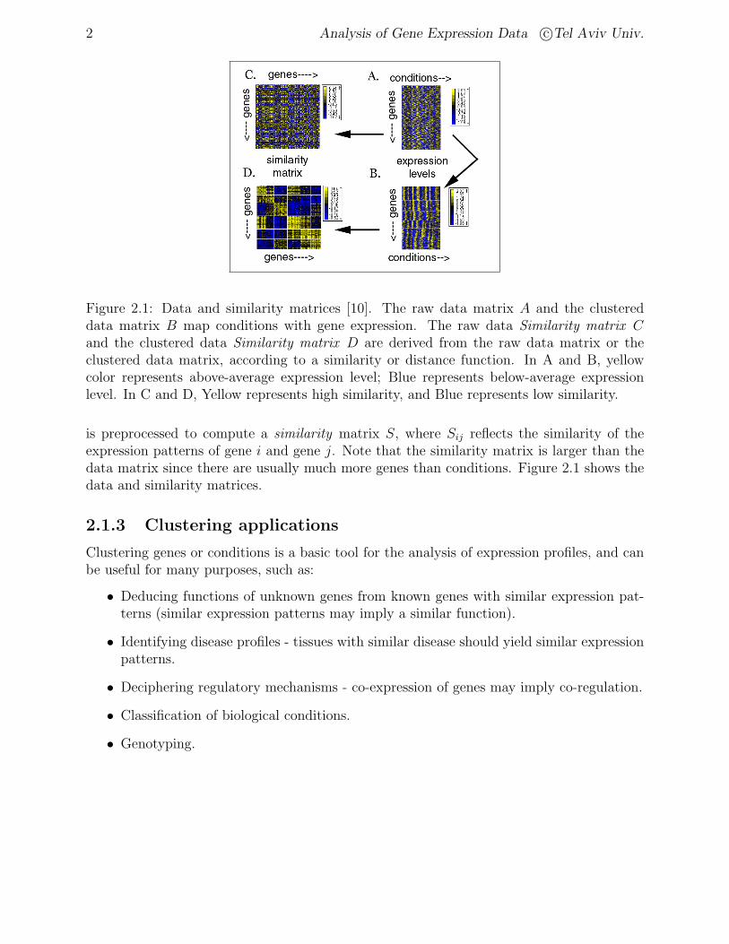
Figure 2.1: Data and similarity matrices [10]. The raw data matrix A and the clustereddata matrix B map conditions with gene expression. The raw data Similarity matrix Cand the clustered data Similarity matrix D are derived from the raw data matrix or theclustered data matrix, according to a similarity or distance function. In A and B, yellowcolor represents above-average expression level; Blue represents below-average expressionlevel. In C and D, Yellow represents high similarity, and Blue represents low similarity.

is preprocessed to compute a similarity matrix S, where Sij reflects the similarity of theexpression patterns of gene i and gene j. Note that the similarity matrix is larger than thedata matrix since there are usually much more genes than conditions. Figure 2.1 shows thedata and similarity matrices.

2.1.3 Clustering applications

Clustering genes or conditions is a basic tool for the analysis of expression profiles, and canbe useful for many purposes, such as:

• Deducing functions of unknown genes from known genes with similar expression pat-terns (similar expression patterns may imply a similar function).

• Identifying disease profiles - tissues with similar disease should yield similar expressionpatterns.

• Deciphering regulatory mechanisms - co-expression of genes may imply co-regulation.

• Classification of biological conditions.

• Genotyping.

Introduction 3

• Drug development.

• And more ...

2.1.4 The Clustering Problem

Genes are said to be similar if their expression patterns resemble, and non-similar otherwise.The goal of gene clustering process is to partition the genes into distinct sets such that genesthat are assigned to the same cluster should be similar, while genes assigned to differentclusters should be non-similar. Usually there is no single solution that is the ”true”/correctmathematical solution for this problem. A good clustering solution should have two merits:

1. Homogeneity : measures the similarity between genes assigned to the same cluster.

2. Separation: measures the distantnce/dis-similarity between the clusters. Each clustershould represent a unique expression pattern. If two clusters have similar expressionpatterns, then probably it would be better to merge them into one cluster.

Note that these two measures are in a way opposite - if you wish to increase the homogeneityof the clusters you would increase the number of clusters, but in the price of reducing theseparation.There are many formulations for the clustering problem, and most of them are NP-hard. Forthat reason, heuristics and approximations are used. Clustering methods have been used ina vast number of fields. We can distinguish between two types of clustering methods:

Agglomerative These methods build the clusters by looking at small groups of elementsand performing calculations on them in order to construct larger groups. Hierarchalmethods of this sort will be described in the next lecture.

Divisive A different approach which analyzes large groups of elements in order to dividethe data into smaller groups and eventually reach the desired clusters. We shall seenon hierarchal techniques which use this approach.

There is another way to distinguish between clustering methods:

Hierarchal Here we construct a hierarchy or tree-like structure to see the relationshipbetween entities. The following hierarchal algorithms will be presented in the nextlecture: Neighbor Joining, Average Linkage and a general framework of for hierarchalcluster merging algorithms.

Non Hierarchal In non hierarchial methods, we start with a seed - we choose a centralpoint from the measurements, and measure the distances of other measurements fromthat central point. The following non hierarchal algorithms will be shown here: k-means, SOM, PCC and CAST. The CLICK algorithm will be presented in the nextlecture.


2.2 k-means clustering

This method was introduced by MacQueen [7]. Given a set of n points V = v1, ..., vn,and an integer k, the goal is to find a k-partition of minimal cost. If P implies a partition ofV into k subsets, then a centroid or center of a cluster C is the center of gravity of its set ofpoints pi = (

∑i∈C vi)/|C|. Let Ep be a function that measures the quality of the partition,

the solution cost. The algorithm moves elements between clusters if it improves Ep, andupdates the 2 affected clusters centers. The new location of the center is determined by theremaining elements of the cluster.

k-means clustering :

1. Initialize an arbitrary partition P into k clusters.

2. For cluster j, element i 6∈ j.Ep(i, j) = Cost of the solution if i is moved to cluster j.

3. Pick Ep(r, s) that is minimum.

4. move r to cluster s, if it improves Ep.

5. Repeat until no improvement possible.

Note that this method requires knowledge of k, the number of clusters, in advance. Sincek is fixed, the algorithm aims at optimizing homogeneity, but not separation, i.e., elementsin different clusters can still remain similar.

The most common use of the k-means algorithm is based on the idea of moving elementsbetween two clusters based on their distances to the centers of the different clusters. Thesolution cost function in that case is defined by:

Ep =∑

p

∑i∈p

D(vi, cp)

Where cp is the center of cluster p and D(vi, cp) is the distance of vi from cp.There are some variations of the algorithm involving changing of k. Also there are parallelversions in which we move each element to the cluster with the closest centroid simultane-ously, but then convergence is not guaranteed. The k-means is a greedy algorithm in itsnature and might get stuck at local minimum, but it is simple, easy for implementation andpopular.

Self organizing maps 5

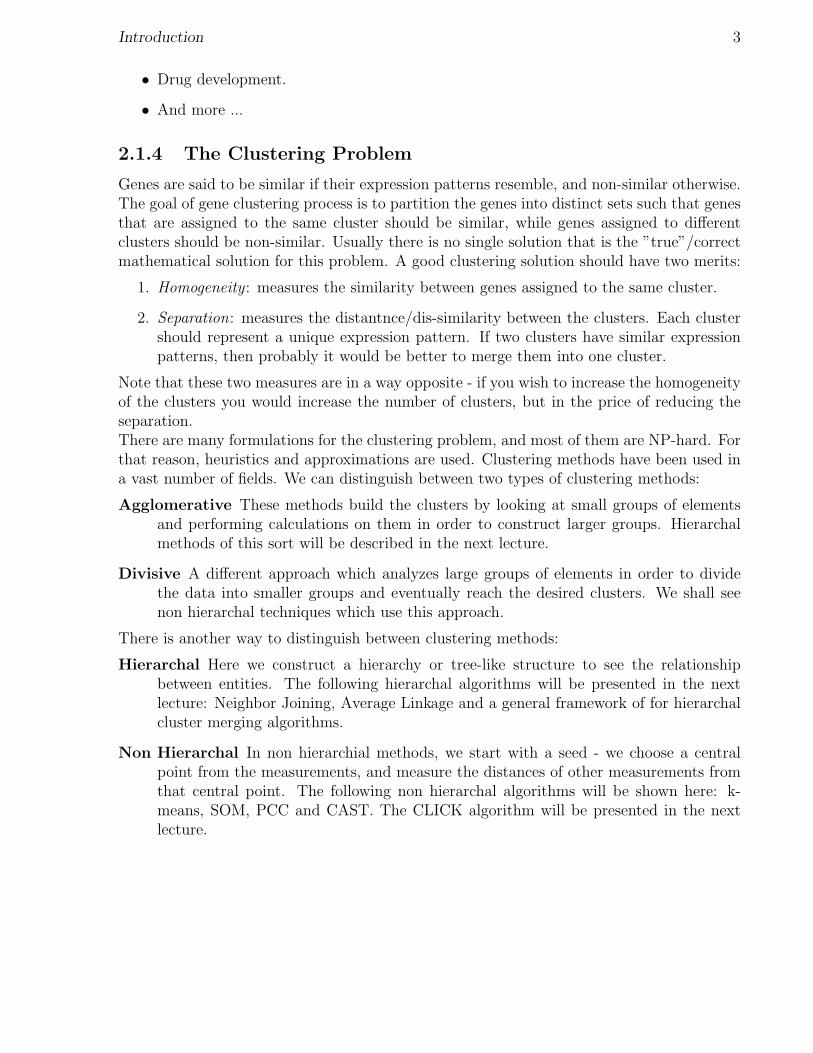
Figure 2.2: Self organizing maps : Initial geometry of nodes in a 3 × 2 rectangular grid isindicated by solid lines connecting the nodes. Hypothetical trajectories of nodes as theymigrate to fit data during successive iterations of the self organizing maps algorithm areshown. Data points are represented by black dots, six nodes of the Self organizing map bylarge circles, and trajectories by arrows.

2.3 Self organizing maps

Kohonen 1997 [6] introduced this method. Tamayo et al [12], applied it to gene expressiondata. Self organizing maps are constructed as follows. k is fixed. Some topology on thecenters is assumed. One chooses a grid, m × n, of nodes, and a Distance function betweennodes, D(N1, N2). Each of the grid nodes is mapped into a k-dimensional space, at random.The gene vectors are mapped into the space as well. As the algorithm proceeds, the gridnodes are iteratively adjusted (See Figure 2.2). Each iteration involves randomly selectinga data point P and moving the grid nodes in the direction of P. The closest node nP ismoved the most, whereas other nodes are moved by smaller amounts depending on theirdistance from nP in the initial geometry. In this fashion, neighboring points in the initialgeometry tend to be mapped to nearby points in k-dimensional space. The process continuesiteratively.

Self organizing maps :

1. Input: n-dim vector for each element (data point) p.

2. Start with a grid of k = l ×m nodes, and a random n-dim associated vector f0(v) foreach grid node v.


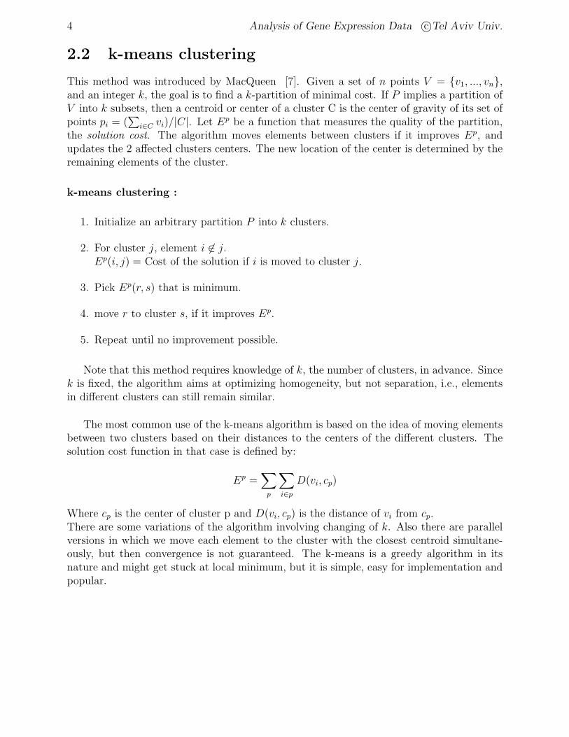
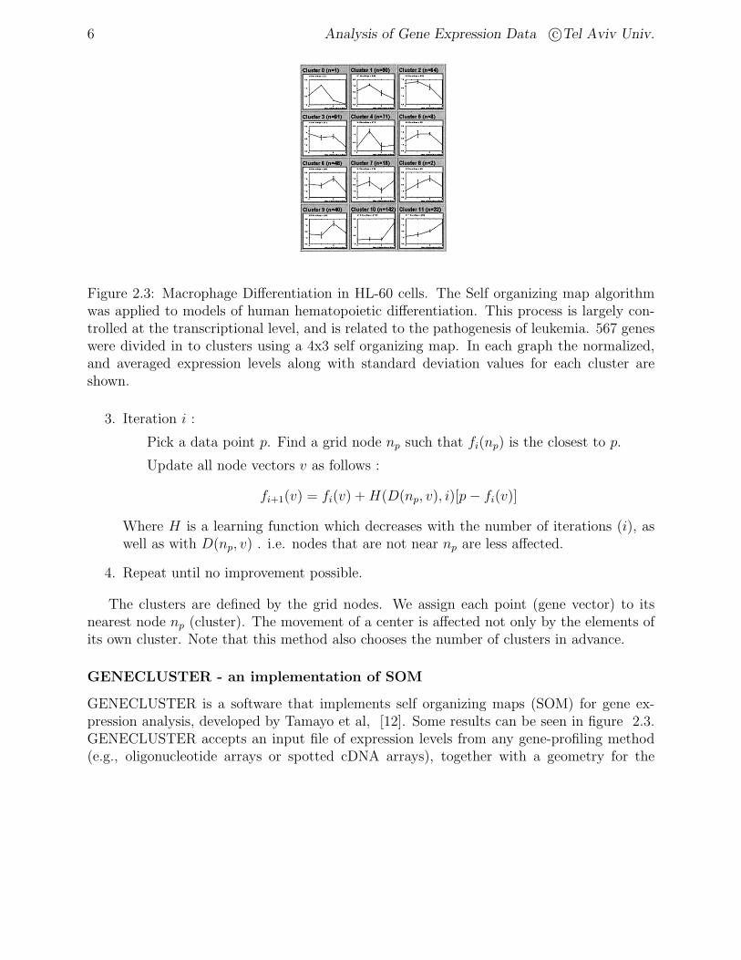
Figure 2.3: Macrophage Differentiation in HL-60 cells. The Self organizing map algorithmwas applied to models of human hematopoietic differentiation. This process is largely con-trolled at the transcriptional level, and is related to the pathogenesis of leukemia. 567 geneswere divided in to clusters using a 4x3 self organizing map. In each graph the normalized,and averaged expression levels along with standard deviation values for each cluster areshown.

3. Iteration i :

Pick a data point p. Find a grid node np such that fi(np) is the closest to p.

Update all node vectors v as follows :

fi+1(v) = fi(v) + H(D(np, v), i)[p− fi(v)]

Where H is a learning function which decreases with the number of iterations (i), aswell as with D(np, v) . i.e. nodes that are not near np are less affected.

4. Repeat until no improvement possible.

The clusters are defined by the grid nodes. We assign each point (gene vector) to itsnearest node np (cluster). The movement of a center is affected not only by the elements ofits own cluster. Note that this method also chooses the number of clusters in advance.

GENECLUSTER - an implementation of SOM

GENECLUSTER is a software that implements self organizing maps (SOM) for gene ex-pression analysis, developed by Tamayo et al, [12]. Some results can be seen in figure 2.3.GENECLUSTER accepts an input file of expression levels from any gene-profiling method(e.g., oligonucleotide arrays or spotted cDNA arrays), together with a geometry for the

Graph Clustering Approaches 7

nodes. The program begins with two preprocessing steps that greatly improve the ability todetect meaningful patterns. First, the data is passed through a variation filter to eliminatethose genes with no significant change across the samples. This prevents nodes from beingattracted to large sets of invariant genes. Second, the expression level of each gene is normal-ized across experiments. This focuses attention on the shape of expression patterns ratherthan on absolute levels of expression. A SOM is then computed. Each cluster is representedby its average expression pattern along with the standard deviation values (see Figure 2.3),making it easy to discern similarities and differences among the patterns. The followinglearning function H(n,r,i) is used, where n and r are nodes, and i stands for iteration:

H(n, r, i) =

0.02T

T+100iif D(n, r) ≤ ρ(i)

0 otherwise

Radius ρ(i) decreases linearly with i (ρ(0) = 3, ρ(T ) = 0). T is the maximum number ofiterations, and D(n,r) denotes the distance within the grid.

2.4 Graph Clustering Approaches

The similarity matrix can be transformed into a similarity graph, Gθ, where the vertices aregenes (i, j), and there is an edge between two vertices if their similarity Si,j is above somethreshold θ. That is, (i, j) ∈ E(Gθ) iff Si,j > θ.

2.4.1 The Corrupted Clique Graph Model

The clustering problem can be modeled by a corrupted clique graph. A clique graph is agraph consisting of disjoint cliques. The true clustering is represented by a clique graphH (vertices are genes and cliques are clusters). Contamination errors introduced into geneexpression data result in a similarity graph C(H) which is not a clique graph. Under thismodel the problem of clustering is as follows: given C(H), restore the original clique graphH and thus the true clustering.

Graph Theoretic Approach

A model for the clustering problem can be reduced to clique graph edge modification prob-lems, stated as follows.

Problem 2.1 Clique graph editing problemINPUT: G(V, E) a graph.OUTPUT: Q(V, F ) a clique graph which minimizes the size of the symmetrical differencebetween the two edge sets: |E∆F |.


Clique graph editing problem is NP-hard [11].

Problem 2.2 Clique graph completion problemINPUT: G(V, E) a graph.OUTPUT: Q(V, F ) a clique graph with E ⊆ F which minimizes |F \ E|.

The clique graph completion problem can be solved by finding all connected componentsof the input graph and adding all missing edges in each component. Thus the clique graphcompletion problem is polynomial.

Problem 2.3 Clique graph deletion problemINPUT: G(V, E) a graph.OUTPUT: Q(V, F ) a clique graph with F ⊆ E which minimizes |E \ F |.

The clique graph deletion problem is NP-hard [8]. Moreover, any constant factor approx-imation to the clique graph deletion problem is NP-hard as well [11].

Probabilistic Approach

Another approach is to build a probabilistic model of contamination errors and try to de-vise an algorithm which, given C(H), reconstructs the original clique graph H with highprobability.

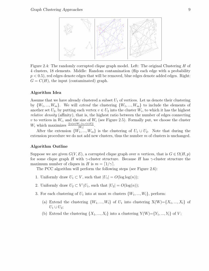
One of the simplest probabilistic models for contamination errors is a random corruptedclique graph. The contamination errors are represented by randomly removing each edge inthe original clique graph H, with probability p < 0.5, and adding each edge not in H withthe same probability, p (see Figure 2.4). We will denote by Ω(H, p) the set of all corruptedclique graphs derived from H with contamination error fraction p using this model.

2.4.2 Probabilistic Clustering Algorithm

In this section we present a clustering algorithm of Ben-Dor et. al. [2], called ParallelClassification with Cores (PCC). We begin with a few definitions.

Definition A cluster structure is a vector (s1, ..., sd), where each sj > 0 and∑

sj = 1.An n-vertex clique graph has structure (s1, ..., sd) if it consists of d disjoint cliques of sizesns1, ..., nsd.

Definition A clique graph H(V, E) is called γ-clustering (has γ-cluster structure), if thesize of each clique in H is at least γ|V |.


Figure 2.4: The randomly corrupted clique graph model. Left: The original Clustering H of4 clusters, 18 elements. Middle: Random contamination (flip each edge with a probabilityp < 0.5), red edges denote edges that will be removed, blue edges denote added edges. Right:G = C(H), the input (contaminated) graph.

Algorithm Idea

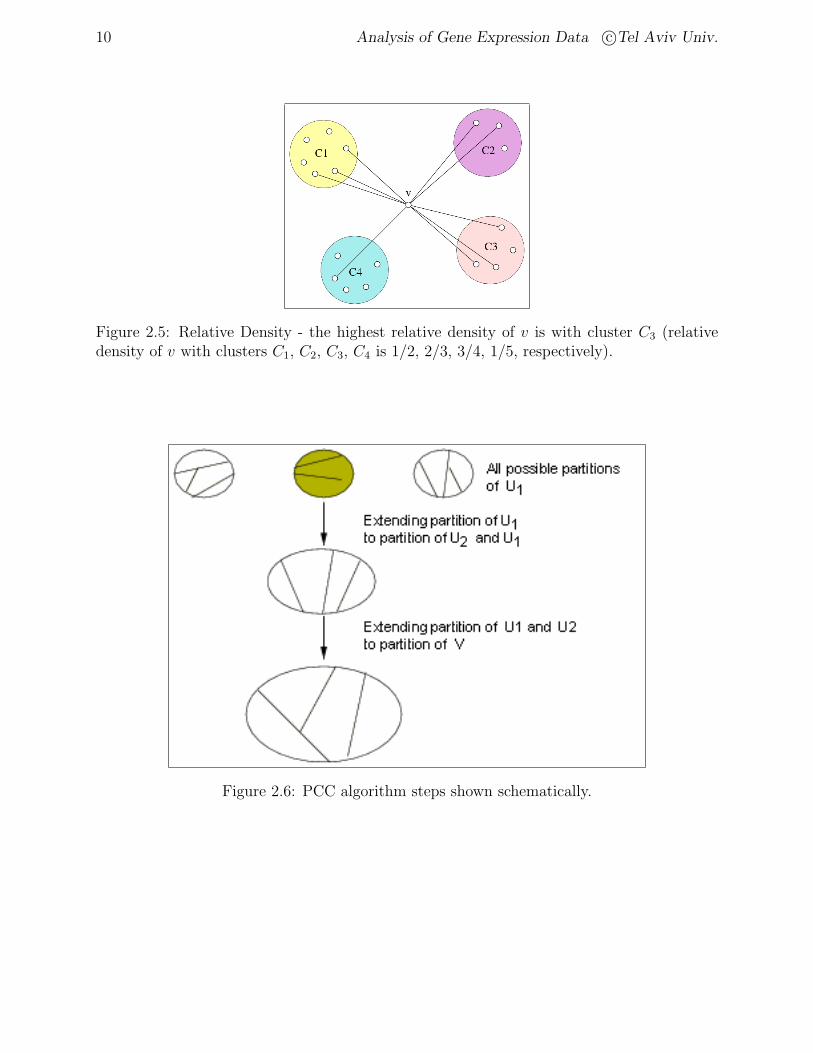
Assume that we have already clustered a subset U1 of vertices. Let us denote their clusteringby W1, ...,Wm. We will extend the clustering W1, ...,Wm to include the elements ofanother set U2, by putting each vertex v ∈ U2 into the cluster Wi, to which it has the highestrelative density (affinity), that is, the highest ratio between the number of edges connectingv to vertices in Wi, and the size of Wi (see Figure 2.5). Formally put, we choose the cluster

Wi which maximizes |u|u∈Wi,(u,v)∈E||Wi| .

After the extension W1, ...,Wm is the clustering of U1 ∪ U2. Note that during theextension procedure we do not add new clusters, thus the number m of clusters is unchanged.

Algorithm Outline

Suppose we are given G(V, E), a corrupted clique graph over n vertices, that is G ∈ Ω(H, p)for some clique graph H with γ-cluster structure. Because H has γ-cluster structure themaximum number of cliques in H is m = d1/γe.

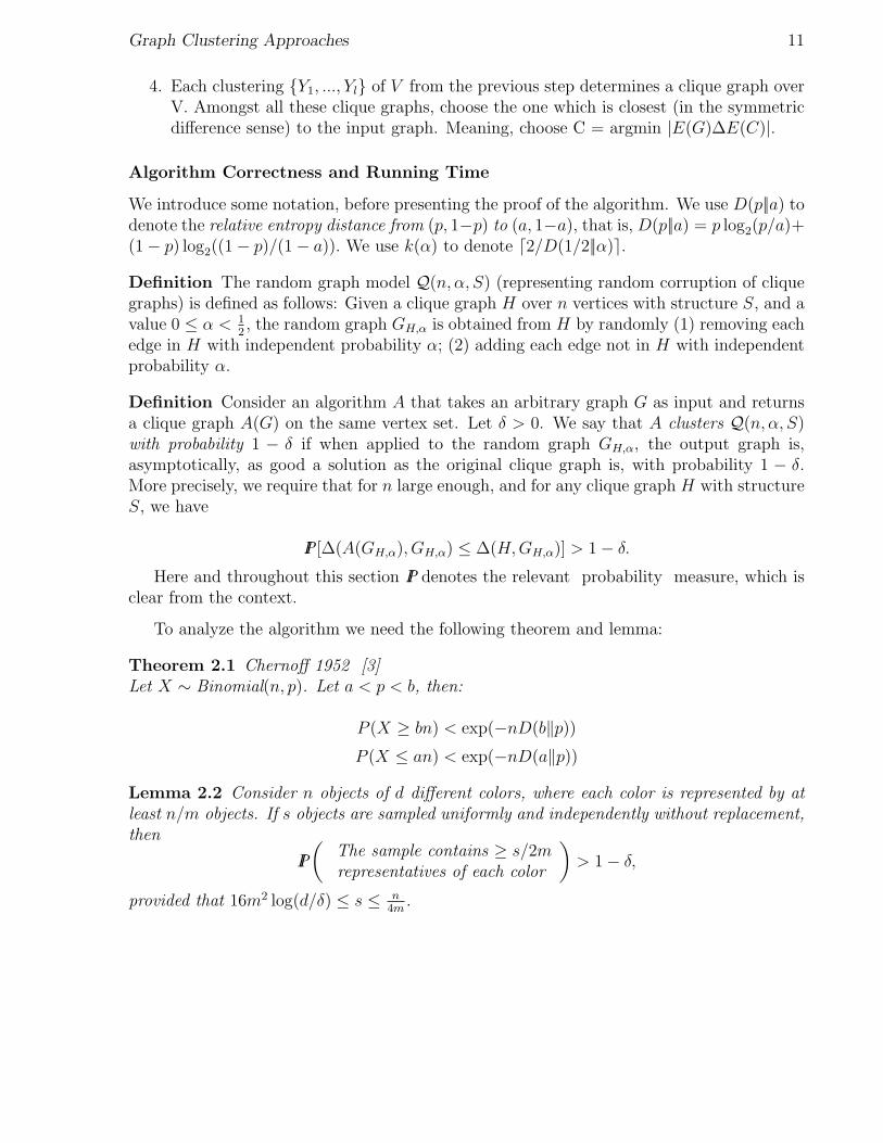
The PCC algorithm will perform the following steps (see Figure 2.6):

1. Uniformly draw U1 ⊂ V , such that |U1| = O(log log(n));

2. Uniformly draw U2 ⊂ V \U1, such that |U2| = O(log(n));

3. For each clustering of U1 into at most m clusters W1, ...,Wl, perform:

(a) Extend the clustering W1, ...,Wl of U1 into clustering X(W)=X1, ..., Xl ofU1 ∪ U2;

(b) Extend the clustering X1, ..., Xl into a clustering Y(W)=Y1, ..., Yl of V ;


Figure 2.5: Relative Density - the highest relative density of v is with cluster C3 (relativedensity of v with clusters C1, C2, C3, C4 is 1/2, 2/3, 3/4, 1/5, respectively).

Figure 2.6: PCC algorithm steps shown schematically.


4. Each clustering Y1, ..., Yl of V from the previous step determines a clique graph overV. Amongst all these clique graphs, choose the one which is closest (in the symmetricdifference sense) to the input graph. Meaning, choose C = argmin |E(G)∆E(C)|.

Algorithm Correctness and Running Time

We introduce some notation, before presenting the proof of the algorithm. We use D(p||a) todenote the relative entropy distance from (p, 1−p) to (a, 1−a), that is, D(p||a) = p log2(p/a)+(1− p) log2((1− p)/(1− a)). We use k(α) to denote d2/D(1/2||α)e.

Definition The random graph model Q(n, α, S) (representing random corruption of cliquegraphs) is defined as follows: Given a clique graph H over n vertices with structure S, and avalue 0 ≤ α < 1

2, the random graph GH,α is obtained from H by randomly (1) removing each

edge in H with independent probability α; (2) adding each edge not in H with independentprobability α.

Definition Consider an algorithm A that takes an arbitrary graph G as input and returnsa clique graph A(G) on the same vertex set. Let δ > 0. We say that A clusters Q(n, α, S)with probability 1 − δ if when applied to the random graph GH,α, the output graph is,asymptotically, as good a solution as the original clique graph is, with probability 1 − δ.More precisely, we require that for n large enough, and for any clique graph H with structureS, we have

PI [∆(A(GH,α), GH,α) ≤ ∆(H, GH,α)] > 1− δ.

Here and throughout this section PI denotes the relevant probability measure, which isclear from the context.

To analyze the algorithm we need the following theorem and lemma:

Theorem 2.1 Chernoff 1952 [3]Let X ∼ Binomial(n, p). Let a < p < b, then:

P (X ≥ bn) < exp(−nD(b‖p))

P (X ≤ an) < exp(−nD(a‖p))

Lemma 2.2 Consider n objects of d different colors, where each color is represented by atleast n/m objects. If s objects are sampled uniformly and independently without replacement,then

PI

(The sample contains ≥ s/2mrepresentatives of each color

)> 1− δ,

provided that 16m2 log(d/δ) ≤ s ≤ n4m

.


Proof:Call a sample as above bad if it does not satisfy the condition for a fixed color A.

p = PI ( bad sample ) ≤ PI (X < s/2m) ,

where X ∼ Binomial(s, (n/m)−s

n

). This is true since even with no replacement the proportion

of A-colored elements left in the pile in each trial is more than (n/m)−sn

. Therefore, by theChernoff bound above, and assuming n > 4ms,

p < exp

(−s ·D(

1

2m|| 3

4m)

)(2.1)

≤ exp

(− s

16 log(2)m2

).

The inequality in (2.2) follows from the general inequality [4]: D(p||q) ≥ (1/ln(2)) · (p− q)2.This last expression is less than δ/d by our assumption on the sample size s. A union overall colors yields the stated result.

Theorem 2.3 Let S be a cluster structure and let α < 1/2. For any fixed δ > 0 the abovealgorithm clusters Q(n, α, S) with probability 1− δ. The time complexity of the algorithm isO (n2 · log(n)c), where c is a constant that depends on α and on γ(S).

Proof:Since m = d 1

γ(S)e, d(S) ≤ m. m is considered a constant for our setup. Let T =

〈T1, . . . Tm〉 be the partition of V that represents the underlying clusters, where some clustersmay be empty. For a vertex v ∈ V let i(T, v) be defined by v ∈ Ti(T,v). Let η > 0 (η will berelated to the tolerated failure probability, δ, at the end). Recall that k(α) = d2/D(1/2||α)e.

1. Uniformly draw a subset U1 of vertices of size 2m · k(α) log log(n). If n is largeenough, namely: log log(n) > 8mk(α) log(1/η) and n > 8m2k(α) log log(n) we know(by Lemma 2.2) that with probability 1 − η each color has at least k(α) log log(n)representatives in this chosen subset.

2. Uniformly over the subsets of V \U1 draw a subset U2 of vertices with 2m · k(α) log(n)elements. Again, for n large enough, with probability 1 − η each color has at leastk(α) log(n) representatives in this subset.

3. Consider all partitions of U1 into m subsets (for n large enough there are less thanlog(n)2m log(m)·k(α) of them). Denote each such partition by W = 〈W1, . . . ,Wm〉 (some


subsets may be empty). Run the following enumerated steps starting with all thesepartitions. For the analysis focus on a partition where each Wi is a subset of a distincttrue cluster Tj.

Such a partition is, indeed, considered, since we are considering all partitions. For thiscase we can further assume, without loss of generality, that for each i we have Wi ⊂ Ti.

(a) Start with sets Xi = Wi. For all u ∈ U2 let i(X, u) be the index that attains themaximum (1 ≤ i ≤ m) of deg(u, Wi)/|Wi|. Add u to that set. Let W (u) = Wi(T,u).

The collection of edges from u to W (u) are independent Bernoulli(1−α) (the draw-ings of U1 and U2 were independent of everything else). Therefore deg(u, W (u)) ∼Binomial(|W (u)|, 1−α). Using the Chernoff bound stated above we therefore have

PI

(deg(u, W (u)) ≤ |W (u)|

2

)< exp(−|W (u)|D(

1

2||α))

< log(n)−k(α)D( 12||α) (2.2)

< log(n)−2, (2.3)

where |W (u)| ≥ k(α) log log(n) justifies (2.2). Similarly, for i 6= i(T, u), we have

deg(u, Wi) ∼ Binomial(|Wi|, α),

and thus

PI (deg(u, Wi) ≥ |Wi|/2) < exp(−|Wi|D(1

2||α))

< log(n)−2, (2.4)

whence i(X, u) = i(T, u) with high probability: PI (i(X, u) 6= i(T, u)) < m log(n)−2.Finally, by a union bound

PI (i(X, u) 6= i(T, u) for some u ∈ U2 ) < 2m2 · k(α) log(n)−1. (2.5)

(b) Focusing on the part of the measure space where no error was committed in theprevious steps (in particular, all vertices were assigned to their original color),we now have m subsets of vertices Xi ⊂ Ti, i = 1...m, each of size at leastk(α) log(n), unless the corresponding Ti is empty. We take all other verticesand classify them using these subsets, as in the previous step. Let the resultingpartition be Y == 〈Y1, . . . , Ym〉 and for vertices v ∈ V let i(Y, v) be defined by


v ∈ Yi(Y,v). Observe that all edges used in this classification are independent of thealgebra generated by everything previously done. This is true since in the previousstep only edges from U2 to U1 were considered, and these are of no interest here.Therefore, the equivalents of (2.3) and (2.4) hold, yielding

PI (i(Y, v) 6= i(T, v) for any v ∈ V ) < 2m2 · k(α)n−1. (2.6)

4. Amongst all outputs of the above, choose the partition which is closest (in the sym-metric difference sense) to the input graph.

The total probability of failure in this process is estimated as follows

PI

(The original partition V =

⋃mi=1 Ti

is not one of the outputs

)≤ 2η + 2m2 · k(α)

(n−1 + log(n)−1

), (2.7)

which is arbitrarily small for large n and if η is chosen appropriately.As noted above, we have less than log(n)2m log(m)·k(α) possible partitions of U1. Each such

partition leads to a clustering of all vertices in V , using the core clusters Xi , i = 1...m.For each partition O(n log(n)) edges are considered in the classification step. Each edge isconsidered at most once, as sums of disjoint edge subsets are compared to a threshold. Com-puting the distance of each of the clique graphs produced to the input graph requires O(n2)operations. Thus the total time complexity of the algorithm is O(n2 · log(n)2m log(m)·k(α)).

2.4.3 Practical Heuristic - Algorithm CAST

Although the theoretical ideas presented in the previous section show asymptotic runningtime complexity of O(n2 logc n), their implementation is still impractical (the constants, forinstance, are very large, as in the computation of all possible partitions of U1 into at mostm clusters in step 3). Therefore, based on ideas of the theoretical algorithm, CAST (ClusterAffinity Search Technique), a simple and practical heuristic, was developed. All the testsdescribed in subsequent sections were performed using this practical implementation of thetheoretical algorithm.Suppose we are given G(V, E), a corrupted clique graph over n vertices, that is G ∈ Ω(H, p)for some clique graph H. Let C be a cluster. Let Si,j be a similarity matrix and let v ∈ V

be a gene. We define the affinity of v to cluster C byP

u∈C Su,v

|C| . Given an affinity thresholdτ we will say that v is a close gene to cluster C if its affinity to C is above τ and we willsay that v is a weak gene in C if its affinity to C is below τ . Following are the steps of thepractical implementation. Repeat the following until all genes are clustered:


• Start a new cluster at a time by picking an unclustered gene, and denote it by CC.As long as changes occur, repeat the following steps:

– Add a close gene to CC;

– Remove a weak gene from CC;

Close CC when no addition or removal is possible;

The main differences between the practical implementation and the theoretical algorithmare:

1. In the theoretical algorithm several partitions are formed and then the “best” partitionis chosen. The clusters in a partition are extended by adding new elements to them.In the practical implementation one partition is formed by building one cluster at atime, and removal of weak elements from a cluster is allowed. This enables correctionin case the seed of the forming cluster is wrong.

2. The theoretical algorithm considers the similarity graph, while the practical implemen-tation processes the similarity matrix (the similarity value between any two genes canassume any real value).

3. In the theoretical algorithm addition is done independently, while the practical imple-mentation adds genes incrementally.

Although little can be proved about the running time and performance of the practi-cal implementation, the test results described in the next sections show that it performsremarkably well, both on simulated data and on real biological data.

BioClust

BioClust is an implementation package of the CAST heuristic. The following section presentsresults of applying BioClust on both synthetic data and real gene expression data.

Clustering Synthetic Data

The simulation procedure is as follows (please refer to Figure 2.7 A for visualization of thesimulation procedure):

• Let H be the original clique graph.

• Generate G from H by independently removing each edge in H with probability p andadding each edge not in H with probability p.


cluster structure n p matching coeff. Jaccard coeff.0.4, 0.2, 0.1× 4 500 0.2 1.0 1.00.4, 0.2, 0.1× 4 500 0.3 0.999 0.9950.4, 0.2, 0.1× 4 500 0.4 0.939 0.7750.1× 10 1000 0.3 1.0 1.00.1× 10 1000 0.35 0.994 0.943

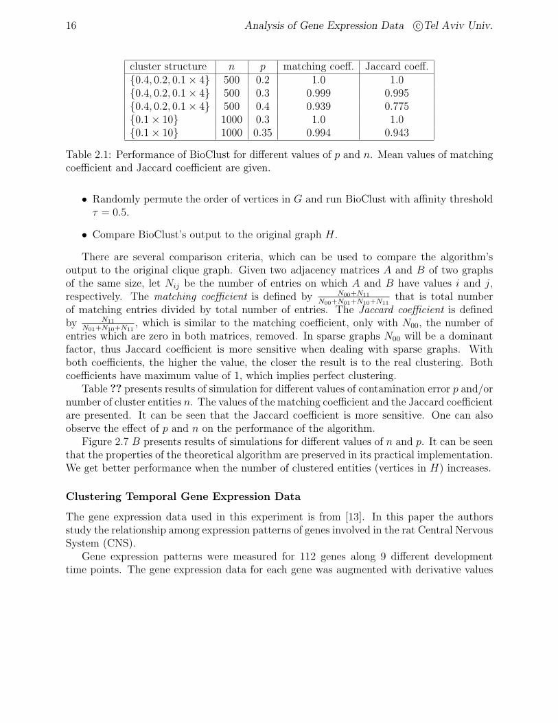
Table 2.1: Performance of BioClust for different values of p and n. Mean values of matchingcoefficient and Jaccard coefficient are given.

• Randomly permute the order of vertices in G and run BioClust with affinity thresholdτ = 0.5.

• Compare BioClust’s output to the original graph H.

There are several comparison criteria, which can be used to compare the algorithm’soutput to the original clique graph. Given two adjacency matrices A and B of two graphsof the same size, let Nij be the number of entries on which A and B have values i and j,respectively. The matching coefficient is defined by N00+N11

N00+N01+N10+N11that is total number

of matching entries divided by total number of entries. The Jaccard coefficient is definedby N11

N01+N10+N11, which is similar to the matching coefficient, only with N00, the number of

entries which are zero in both matrices, removed. In sparse graphs N00 will be a dominantfactor, thus Jaccard coefficient is more sensitive when dealing with sparse graphs. Withboth coefficients, the higher the value, the closer the result is to the real clustering. Bothcoefficients have maximum value of 1, which implies perfect clustering.

Table ?? presents results of simulation for different values of contamination error p and/ornumber of cluster entities n. The values of the matching coefficient and the Jaccard coefficientare presented. It can be seen that the Jaccard coefficient is more sensitive. One can alsoobserve the effect of p and n on the performance of the algorithm.

Figure 2.7 B presents results of simulations for different values of n and p. It can be seenthat the properties of the theoretical algorithm are preserved in its practical implementation.We get better performance when the number of clustered entities (vertices in H) increases.

Clustering Temporal Gene Expression Data

The gene expression data used in this experiment is from [13]. In this paper the authorsstudy the relationship among expression patterns of genes involved in the rat Central NervousSystem (CNS).

Gene expression patterns were measured for 112 genes along 9 different developmenttime points. The gene expression data for each gene was augmented with derivative values


to enhance the similarity for closely parallel but offset expression patterns, resulting in a112 × 17 expression matrix. The similarity matrix was obtained using Euclidean distance.The execution of BioClust resulted in eight clusters. Since partitioning to clusters is knownfrom [13] this experiment was done mainly for validation of the algorithm.

Figure 2.7 C and D presents the clustering results. Note that all clusters, perhaps withthe exception of cluster #1, manifest clear and distinct expression patterns. Moreover, theagreement with the prior biological classification is quite good.

Clustering C. Elegans Gene Expression Data

The gene expression data used in this analysis is from [5]. Kim et al. studied gene regulationmechanisms in the nematode C. Elegans. Gene expression patterns were measured for 1246genes in 146 experiments, resulting in a 1246×146 expression matrix. The similarity matrixwas obtained using Pearson correlation.

The algorithm found 40 clusters. Only very few genes out of the 1246 were classified intofamilies by prior biological studies. The algorithm clustered these families quite well intofew homogeneous clusters (see Figure 2.8).

One example of the potential use of clustering for analyzing gene expression patterns isshown in Figure 2.8. A six-gene cluster (cluster #24) contained two growth-related genesand four anonymous genes. This suggests the possibility that the other four genes are alsogrowth-related, paving the way for future biological research.

Tissue Clustering

The gene expression data used in this experiment is from [1]. The authors describe ananalysis of gene expression data obtained from 62 samples of colon tissue, 40 tumor and 22normal tissues. Gene expression patterns were measured for 2000 genes in the 62 samples,using an Affymetrix chip. The similarity between each two samples was measured usingPearson correlation. Note that here, the similarity is measured between tissues, not genes.

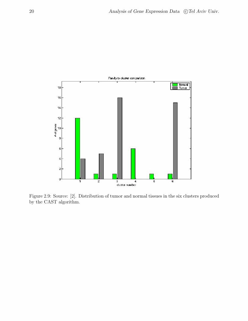
BioClust formed 6 clusters of the data. Figure 2.9 shows the distribution of tumor andnormal tissues in the six clusters produced.

The main goal of clustering here is to achieve a separation of tumor and normal tissues.This experiment demonstrates the usefulness of clustering techniques in learning more aboutthe relationship of expression profiles to tissue types.

Improved Theoretical Results

Shamir & Tsur [9] have introduced a generalized random clique graph model with improvedtheoretical results, including reduction of the Ω(n) restriction on cluster sizes, and strongerresults when cluster sizes are almost equal.


a b

c dA B

C D

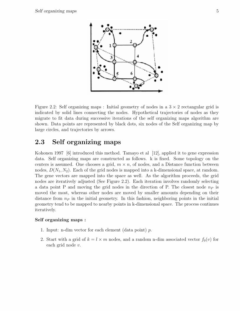
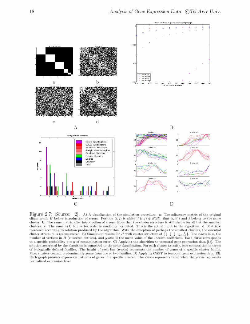
Figure 2.7: Source: [2]. A) A visualization of the simulation procedure. a: The adjacency matrix of the originalclique graph H before introduction of errors. Position (i, j) is white if (i, j) ∈ E(H), that is, if i and j belong to the samecluster. b: The same matrix after introduction of errors. Note that the cluster structure is still visible for all but the smallestclusters. c: The same as b but vertex order is randomly permuted. This is the actual input to the algorithm. d: Matrix creordered according to solution produced by the algorithm. With the exception of perhaps the smallest clusters, the essentialcluster structure is reconstructed. B) Simulation results for H with cluster structure of 1

2, 14, 18, 116

, 116

. The x-axis is n, thenumber of vertices in H (clustered entities), and y-axis is the mean value of the Jaccard coefficient. Each curve correspondsto a specific probability p = α of contamination error. C) Applying the algorithm to temporal gene expression data [13]. Thesolution generated by the algorithm is compared to the prior classification. For each cluster (x-axis), bars composition in termsof biologically defined families. The height of each bar (y-axis) represents the number of genes of a specific cluster family.Most clusters contain predominantly genes from one or two families. D) Applying CAST to temporal gene expression data [13].Each graph presents expression patterns of genes in a specific cluster. The x-axis represents time, while the y-axis representsnormalized expression level.


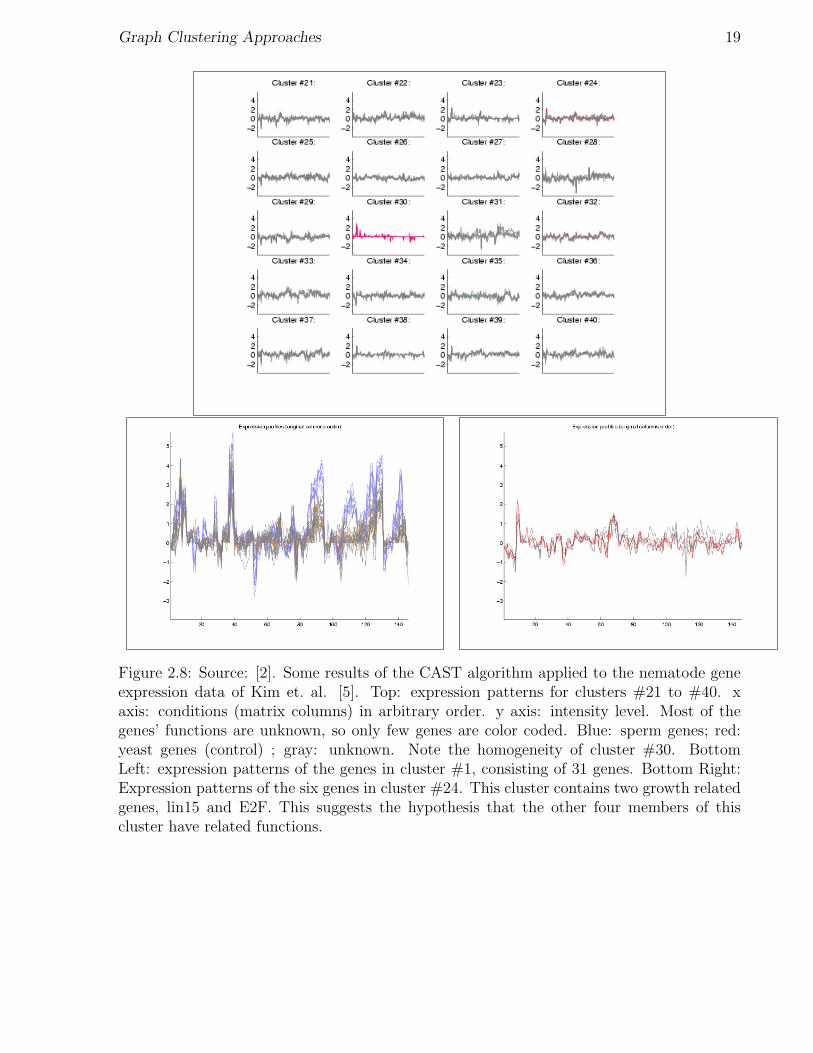
Figure 2.8: Source: [2]. Some results of the CAST algorithm applied to the nematode geneexpression data of Kim et. al. [5]. Top: expression patterns for clusters #21 to #40. xaxis: conditions (matrix columns) in arbitrary order. y axis: intensity level. Most of thegenes’ functions are unknown, so only few genes are color coded. Blue: sperm genes; red:yeast genes (control) ; gray: unknown. Note the homogeneity of cluster #30. BottomLeft: expression patterns of the genes in cluster #1, consisting of 31 genes. Bottom Right:Expression patterns of the six genes in cluster #24. This cluster contains two growth relatedgenes, lin15 and E2F. This suggests the hypothesis that the other four members of thiscluster have related functions.


Figure 2.9: Source: [2]. Distribution of tumor and normal tissues in the six clusters producedby the CAST algorithm.

Bibliography

[1] U. Alon, N. Barkai, D. A. Notterman, G. Gish, S. Ybarra, D. Mack, and A. J. Levine.Broad patterns of gene expression revealed by clustering analysis of tumor and normalcolon tissues probed by oligonucleotide arrays. PNAS, 96:6745–6750, June 1999.

[2] A. Ben-Dor, R. Shamir, and Z. Yakhini. Clustering gene expression patterns. Journalof Computational Biology, 6(3/4):281–297, 1999.

[3] H. Chernoff. A measure of the asymptotic efficiency for tests of a hypothesis based onthe sum of observations. Annals of Mathematical Statistics, 23:493–509, 1952.

[4] T. M. Cover and J. M. Thomas. Elements of Information Theory. John Wiley & Sons,London, 1991.

[5] S. Kim. Department of Developmental Biology, Stanform University,http://cmgm.stanford.edu/∼kimlab/.

[6] T. Kohonen. Self-Organizing Maps. Springer, Berlin, 1997.

[7] J. MacQueen. Some methods for classification and analysis of multivariate observa-tions. In Proceedings of the 5th Berkeley Symposium on Mathematical Statistics andProbability, pages 281–297, 1965.

[8] A. Natanzon. Complexity and approximation of some graph modification problems.Master’s thesis, Department of Computer Science, Tel Aviv University, 1999.

[9] R. Shamir and D. Tsur. Improved algorithms for the random cluster graph model. InProc. 8th Scandinavian Workshop on Algorithm Theory (SWAT ’02), LNCS 2368, pages230–239. Springer-Verlag, 2002.

[10] R. Sharan, A. Maron-Katz, N. Arbili, and R. Shamir. EXPANDER: EXPres-sion ANalyzer and DisplayER, 2002. Software package, Tel-Aviv University,http://www.cs.tau.ac.il/∼rshamir/expander/expander.html.

21

22 BIBLIOGRAPHY

[11] R. Sharan, R. Shamir, and D. Tsur. Cluster graph modification problems. In Proc. 28thInternational Workshop on Graph-Theoretic Concepts in Computer Science (WG ’02),To appear.

[12] P. Tamayo, D. Slonim, J. Mesirov, Q. Zhu, S. Kitareewan, E. Dmitrovsky, E. S. Lander,and T.R. Golub. Interpreting patterns of gene expression with self-organizing maps:Methods and application to hematopoietic differentiation. PNAS, 96:2907–2912, 1999.

[13] X. Wen, S. Fuhrman, G. S. Michaels, D. B. Carr, S. Smith, J. L. Barker, and R. Somogyi.Large-scale temporal gene expression mapping of central nervous system development.PNAS, 95(1):334–339, 1998.

Documents

Analysis of Gene Expression Data Spring Semester, 2005 ...rshamir/ge/05/scribes/lec02.pdf · Analysis of Gene Expression Data Spring Semester, 2005 Lecture 2: March 03, 2005 Lecturer: