ANALYSIS OF FREE ROAD DATA IN TANZANIA, …...ANALYSIS OF FREE ROAD DATA IN TANZANIA, UGANDA AND KENYA USING FREE AND OPEN SOURCE SOFTWARE Stefan Jovanovic 1, Dina Jovanovic 1, Gorica

ANALYSIS OF FREE ROAD DATA IN TANZANIA, UGANDA AND KENYA

USING FREE AND OPEN SOURCE SOFTWARE

Stefan Jovanovic 1, Dina Jovanovic 1, Gorica Bratic 1, Maria Antonia Brovelli 1, *

1 Politecnico di Milano, Department of Civil and Environmantal Engineering, Piazza Leonardo da Vinci, 20133 Milano, Italy -

(stefan.jovanovic, gorica.bratic, maria.brovelli)@polimi.it, [email protected]

Commission IV, WG IV/4

KEY WORDS: Free and open data, OpenStreetMap, roads, positional accuracy, completeness, road accessibility rate

ABSTRACT:

Roads are one of the most important infrastructural objects for each country. Slow development of third world countries is partially

influenced by missing roads. Therefore, United Nation (UN) enlisted them inside the ninth Sustainable Development Goal (SDG)

whose achievement highly relies on geospatial data. Since the authoritative data for the majority of developing countries are

incomplete and unavailable, the focus of this study is on free data. The conveyed research, explained in this paper, was divided in

two parts. The first one refers to completeness and positional accuracy assessment of three different road data sets (freely available).

The second part was focused only on OpenStreetMap (OSM) since it showed the best results in the previous stage. Thus, OSM was

used to compute (in the second part of the research) and analyse the road accessibility rate within the buffer zone of two kilometers

from human settlements. To locate human settlements, raster data, representing land covers were used. Results are pointing where

the infrastructure is not mapped or is not present. The complete work was done using Free and Open Source Software, which is

important, since the proposed procedure can be implemented by anyone.

* Corresponding author

1. INTRODUCTION

Good infrastructure has a vast effect on the whole sustainable

development of a country, ie. economy, industry and trade. The

efficient road network, is a part of infrastructure that is required

to maximize economic and social benefits of any country

(Ivanova and Masarova, 2013).

The importance of having strong and well-structured network of

roads is also shown through the United Nations’ Sustainable

Development Goals (UN SDGs)

(https://doi.org/10.18356/29c75b3e-en) in which the ninth goal

focuses on Industry, Innovation and Infrastructure. Each SDG

is characterized by indicators that are frameworks for future

actions and analysis. Particularly for goal nine, the indicator

9.1.1 considers the proportion of the rural population who live

within 2 km of all-season roads. This indicator will address

governments, stakeholders, and decision makers where they

should invest in road infrastructure. In order to achieve its

successful computation, as well as the similar ones, geospatial

data related to population and roads are required. Since

collection of those data is demanding, regarding both, money

and time, free and open data were used in this research.

However, before using those roads data for any kind of purpose

their quality has to be examined and secured.

That fact raises the core research questions: “How to analyse

free and open road data and how to accomplish the calculation

of road accessibility rate (RAR)?” More specifically, the study

aimed to achieve the following specific research objectives:

To identify the most reliable free road data source;

To create a workflow for computation of RAR

(similar to SDG indicator 9.1.1) by exploiting just

Free and Open Source Software (FOSS);

To present results applying multi-dimensional

visualization that is understandable for policymakers.

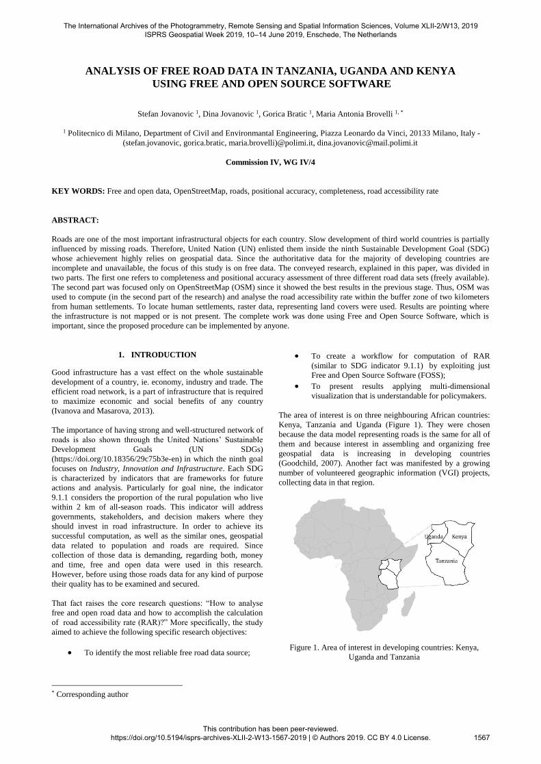
The area of interest is on three neighbouring African countries:

Kenya, Tanzania and Uganda (Figure 1). They were chosen

because the data model representing roads is the same for all of

them and because interest in assembling and organizing free

geospatial data is increasing in developing countries

(Goodchild, 2007). Another fact was manifested by a growing

number of volunteered geographic information (VGI) projects,

collecting data in that region.

Figure 1. Area of interest in developing countries: Kenya,

Uganda and Tanzania

The International Archives of the Photogrammetry, Remote Sensing and Spatial Information Sciences, Volume XLII-2/W13, 2019 ISPRS Geospatial Week 2019, 10–14 June 2019, Enschede, The Netherlands

This contribution has been peer-reviewed. https://doi.org/10.5194/isprs-archives-XLII-2-W13-1567-2019 | © Authors 2019. CC BY 4.0 License.

1567

https://doi.org/10.18356/29c75b3e-en

A good example of VGI project is Crowed2Map Tanzania

(https://crowd2map.wordpress.com). This idea is based on the

crowdsourced mapping, where volunteers are giving their

contribution to Female Genital Mutilation (FGM) prevention by

collecting roads data in rural areas of Tanzania. This leads to

completion and creation of the maps that can, for instance,

guide endangered girls to safe houses.

The research paper is structured as it follows: The first section

introduces the area of interest, methodology and main research

goals. Section 2 reviews related works with similar topics.

Section 3 shows the positional accuracy and completeness

analysis of three roads data sets. The most accurate one was

used in Section 4 to compute the RAR. Section 5 summarizes

the completed work and suggests steps for future researches.

2. RELATED WORKS

The quality analyses of free road data were topic of many

researches. They consist of comparing a free data set (like

OpenStreetMap-OSM) to the other data set (usually

authoritative data or satellite imagery) which is considered as

more accurate (Haklay, 2010). While several studies had the

main focus just on the completeness (Zielstra et al. 2011) other

compared geometries, thematic attributes of road network data

and their positional differences (Ludwig et al., 2011). Siebritz

and Sithole (2014) completed a qualitative and quantitative

comparison between national mapping agency data in South

Africa and OSM. Growing number of free and open data sets

triggered comparative analyses, that can give insight which one

is more reliable and which one is developing faster in terms of

quantity/quality (Mooney and Corcoran, 2014; Neis and Zipf,

2012).

Some researches were focused on the analysis of attributes

assigned to road data (Leitner and Arsanjani, 2017). For

instance, features referring to the seasonality of roads were

useful while investigating access of population to these roads

(Nkomo et al., 2016). According to Vincent (2018), missing

that piece of information partially caused the failure of study,

conveyed by The World Bank Group, that developed Rural

Access Index (equal to SDGs indicator 9.1.1) in 2006.

Free and Open Source Software for Geospatial (FOSS4G) can

be used to assess the quality of open datasets (Brovelli et al.,

2015). These softwares are available to everyone, and they can

also support personalized development of specific extensions

(Martinez-Llario et al., 2009). Using FOSS, the source codes

are available publicly, so they offer higher degree of flexibility

to broader group of users and researchers. (Brovelli et al.,

2016).

3. ANALYSIS OF FREE GEOSPATIAL DATA

The first step in the analysis of Free Geospatial road data in this

research was the evaluation of the completeness and positional

accuracy. Completeness accuracy serves to measure the gap in

data collection. Deficiency of data can cause partial view of the

overall picture. This considers discrepancies between the

evaluated data set and a data set that is considered to have

sufficient completeness (e.g. high-resolution satellite imagery).

“Positional accuracy is a measurement of the variance of map

features and the true position of the attribute (Antenucci et al.,

1991).” Positional accuracy and completeness are included in

both standards: European (CEN, 1995) and US (USGS, 1990),

(Table 1).

Data, that showed the greatest level of positional and

completeness accuracy, were used in the second part of research

for computation of RAR.

European Standard (European Committee for

Standardization/Technical Committees - CEN/TC287)

Lineage

Usage

Quality parameters:

~Primary accuracy:

- Positional accuracy

- Thematic accuracy

- Logical consistency

- Completeness

- Temporal accuracy

~Secondary parameters:

- Textual fidelity

US Standard (Spatial DAta Transfer Standard-SDTS)

Lineage

Positional accuracy

Attribute accuracy

Logical consistency

Completeness

Table 1. Set of European and US Standards for analysis of

geospatial data

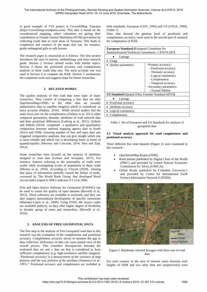
3.1 Visual analysis approach for road completeness and

positional accuracy

Three different free road datasets (Figure 2) were examined in

this research :

OpenStreetMap Roads (OSM);

Road dataset published by Digital Chart of the World

(DWC) and provided by United Nations Economic

Commission for Africa (UNECA);

Global Roads published by Columbia University’s

and provided by Centre for International Earth

Science Information Network (CIESIN).

Figure 2. Randomly selected hexagon with three sets of road

data

For each country in the area of interest ratios between total

lengths of OSM and two other data sets (respectively) were



1568

https://onlinelibrary.wiley.com/doi/full/10.1111/tgis.12182#tgis12182-bib-0020

https://onlinelibrary.wiley.com/doi/full/10.1111/tgis.12182#tgis12182-bib-0021

https://dl.acm.org/author_page.cfm?id=99659194808&coll=DL&dl=ACM&trk=0


https://en.wikipedia.org/wiki/European_Committee_for_Standardization

https://en.wikipedia.org/wiki/European_Committee_for_Standardization

computed. Values presented in Table 2 are giving the first

insight how the completeness differs between these datasets.

COUNTRY TLOSM/TLCIESIN TLOSM/TLDCW

Kenya 2.5 4.5

Tanzania 5.6 7.7

Uganda 6.5 8.0

Table 2. Ratio between OSM and DCW road data and OSM and

CIESIN road data

Yet, to have more reliable information about the completeness,

visual inspection was done. The data to be analysed here are

rather complex, thus they were divided into regular cells i.e.

grid to simplify the procedure. There are various grid shapes,

but only three have regular geometric form (equilateral and

equal internal angles) that ensure continuity in a dataset . They

are: equilateral triangle, square and hexagon. Among these

shapes, the more similar to a circle the polygon is, the closer to

the centroid the points near the border are (Moreira de Sousa

and Leitão, 2017). Therefore, the area of interest was divided in

hexagon grid with the apothem of 10 km that can give enough

data inside boundaries but yet not too large. From total number

of hexagons in all three countries is 4422, a sample of 220

randomly chosen hexagons was used for road data accuracy

estimation, and the following procedure was repeated for each

of them. A hexagon was used to represent a “bounding box”

where three evaluators were checking road data accuracy,

independently of each other. The assessment of the

completeness of features was done by the visual comparison of

road data sets with Bing Aerial imagery (hereafter satellite

imagery) in QGIS.

Before performing visual “inspection”, comparisons between

temporal resolutions of satellite imagery and each road data set

were accomplished.

Under assumption that complete data set does not exist,

evaluators had the opportunity to assign one of the three

attributes representing completeness:

sufficient - existing road data were also visible on

satellite imagery;

excessive - road data existed, but could not be

recognized on satellite imagery;

no data - road data were missing.

The value assigned by at least two evaluators was considered as

the final one for completeness of the data.

Regarding the estimation of positional accuracy, only hexagons

where roads were labeled as sufficient were taken into account.

At first, each evaluator was searching for the feature (usually

crossroad) represented by the road data set which was

recognizable on the satellite imagery. After that, the distance

between same feature in data set and satellite imagery was

assigned as the value for the positional accuracy. Since

evaluators worked individually they chose different features to

measure that distance. Finally, the positional accuracy of

complete road data set was the mean of positional accuracies of

individual hexagons.

3.2 Results of visual analysis approach for road

completeness and positional accuracy

For all datasets majority of hexagons were classified as

‘sufficient’. However, results in Table 3 are proving that OSM

is the most complete, with 219 hexagons as ‘sufficient’ and just

one hexagon classified as “excessive”. CIESIN and DCW

datasets contain 24% and 28% (respectively) hexagons that are

missing data or assigned as “excessive”.

Completeness

OSM

CIESIN DCW

Number of hexagons

Sufficient 219 (99.5%) 173 (76%) 157 (71%)

Excessive 1 (0.5%) 17 (8%) 36 (16%)

No data 0 30 (16%) 27 (12%)

Table 3. Number of hexagons per completeness classes

For each data set the mean value, median and standard

deviation of positional accuracy were computed. Results

presented in Table 4 are pointing out OSM as the positionaly

most accurate dataset.

Indicator

OSM

CIESIN DCW

Number of hexagons 219 173 157

Mean Value of positional

accuracy [m] 35 600 1100

Median of positional

accuracy [m] 20 220 600

Standard deviation of

positional accuracy [m] 45 740 860

Table 4. The basic statistics of positional accuracy

The analysis of statistics showed that OSM road data are the

most reliable for further research. OSM road data are often

enriched by information about road surface. Road surface

categories can be generic, simply distinguishing between natural

and man-made materials (unpaved and paved) on the road

surface. On the other hand, more detailed categorization sets

apart specific materials (e.g. asphalt or gravel), but eventually

they can be assigned to one of the generic categories. In

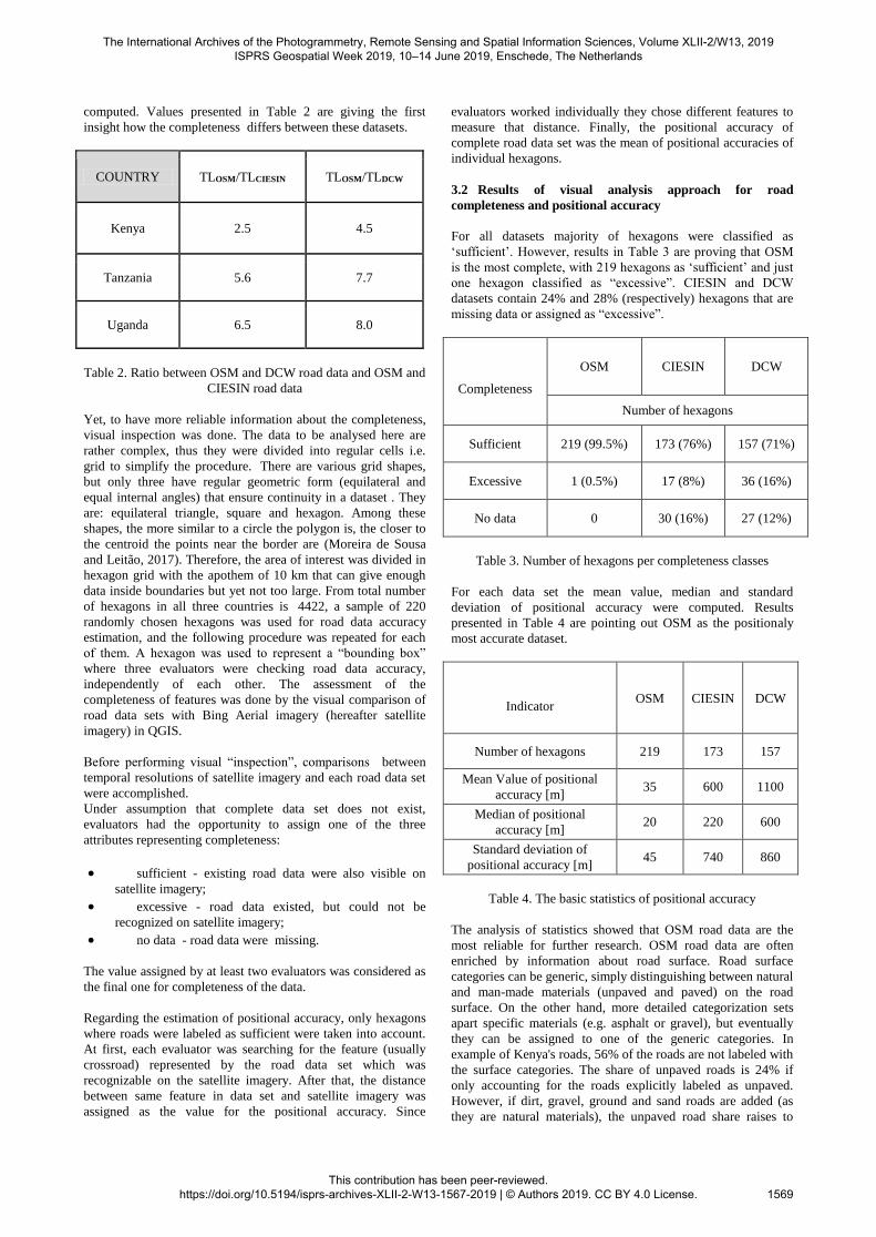
example of Kenya's roads, 56% of the roads are not labeled with

the surface categories. The share of unpaved roads is 24% if

only accounting for the roads explicitly labeled as unpaved.

However, if dirt, gravel, ground and sand roads are added (as

they are natural materials), the unpaved road share raises to



1569

https://onlinelibrary.wiley.com/action/doSearch?ContribAuthorStored=Leit%C3%A3o%2C+Jo%C3%A3o+Paulo

34%. The remaining 10% of the roads in Kenya are paved.

(Figure 3).

Figure 3. Pie chart of surfaces for Kenya's secondary roads

4. ROAD ACCESSIBILITY COMPUTATION USING

LAND COVER RASTERS AND OSM ROAD DATA

Three different rasters were used to extract information about

areas in which there is human footprint (hereafter human

settlement):

Climate Change Initiative - S2 Prototype Land Cover

20m map of Africa 2016 (CCI+);

GlobeLand30 (GL30);

Global Human Settlement Built-Up Grid (GHS).

4.1 Description of the used raster data

CCI+(http://2016africalandcover20m.esrin.esa.int), developed

by European Space Agency (ESA), represents 20 meters

resolution land cover map of Africa based on 1 year of Sentinel-

2A observations from December 2015 to December 2016.

Among 10 generic classes that appropriately describe the land

surface the class Built-up areas is devoted to human settlement.

The Coordinate Reference System used for the CCI+ is a

geographic coordinate system based on the World Geodetic

System 84 (WGS84) reference ellipsoid.

GL30 (http://www.globallandcover.com) is a product of

“Global Land Cover Mapping at Finer Resolution” project led

by the National Geomatics Center of China (NGCC). GL30

refers to land cover of the earth between latitude 80°N to 80°S,

containing 10 classes with different land cover types. Pixels

representing human settlement (PHS) belong to class Artificial

surface and their value is 80. The resolution of GL30 is 30

meters and it adopts WGS84 coordinate system. For this paper,

GL30 from reference year of 2015 was used.

GHS (https://ghsl.jrc.ec.europa.eu/ghs_bu.php), as a part of

Global Human Settlement Layer project, is supported by the

European Commission (EC), Joint Research Center and

Directorate-General for Regional and Urban Policy. GHS is a

38 meter resolution binary raster in which values are expressed

in byte from 1 (for non-built areas) to 101 (for built-up areas),

with 0 representing no data. Data used for this paper refer to

2015 and they are in Spherical Mercator projection.

Table 5 summarizes the provider, the resolution, European

Petroleum Survey Group (EPSG) code, the year of satellite

imagery used to produce land cover map and PHS.

Name Provider Resolution

[m]

EPSG

code Year

PHS

value

CCI+ ESA 20 x 20 4326 2016 8

GL30 NGCC 30 x 30 4326 2015 80

GHS EC 38 x 38 3857 2015 101

Table 5. Characteristics of different raster data

The computation of population density was based on Worldpop

(http://www.worldpop.org.uk) raster, which is a result of

mapping project of numerous universities, agencies and

organizations. This raster, whose resolution is 100 meters,

EPSG 4326, represents distribution of human population for

2015.

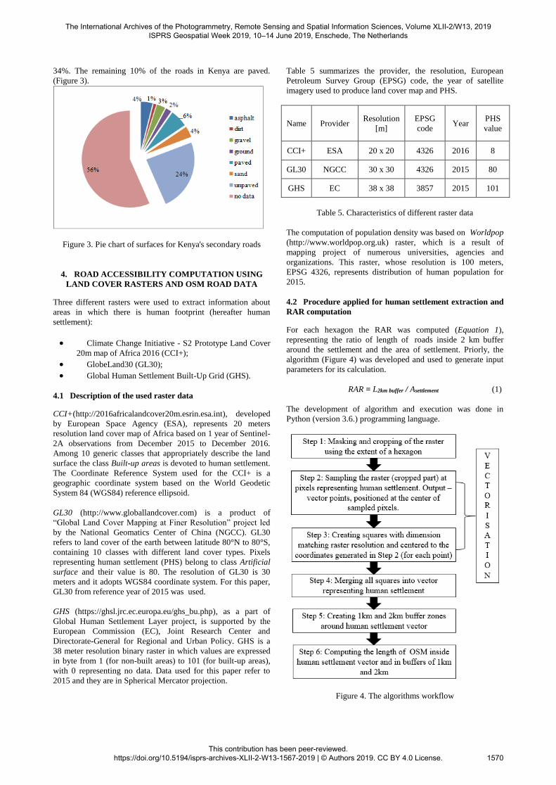
4.2 Procedure applied for human settlement extraction and

RAR computation

For each hexagon the RAR was computed (Equation 1),

representing the ratio of length of roads inside 2 km buffer

around the settlement and the area of settlement. Priorly, the

algorithm (Figure 4) was developed and used to generate input

parameters for its calculation.

RAR = L2km buffer / Asettlement (1)

The development of algorithm and execution was done in

Python (version 3.6.) programming language.

Figure 4. The algorithms workflow



1570

http://2016africalandcover20m.esrin.esa.int/

http://www.worldpop.org.uk/resources/doc

Step 1 is masking and cropping of the raster, by the extent of a

hexagon. Steps 2 and 3 represent process of vectorisation. At

first, the cropped part of raster is sampled at the points

representing human settlement. As a result, vector points

positioned in centers of those pixels are generated. Than,

squares of size equal to the pixel size and centered to the

coordinates are created. By merging the squares (Step 4) the

human settlement is defined and afterwards buffer zones are

built (Step 5). At the end the length of OSM inside settlement

and two buffer zones is computed.

The algorithm includes following Python packages/libraries:

1. Rasterio (GDAL and NumPy Python library for

geospatial raster data access)

2. Shapely (Package for manipulation and analysis of

planar geometric objects)

3. Numpy (Package for scientific computations)

4. Geopandas (Package that enables user to do in

Python that would otherwise require a spatial

database such as PostGIS)

The computation of the surface of the human settlement for

each hexagon (Step 4 - Figure 4), was included in the algorithm

and executed simultaneously with its remainder.

4.3 Results and multidimensional visualization

For multidimensional interpretation of the results, the

Qgis2threejs plugin of QGIS was used. For each hexagon the

value H (Equation 2) was computed, representing the

normalized value of RAR with respect to maximum value of

RAR (for each country and land cover map individually).

H = (RARi / RARmax)*100 (2)

Figure 5. Human settlements "detected" by CCI+ for Uganda

Looking at Figure 5, one can notice different shades of blue.

They are depicting different density of population per square

kilometer. The darker the color is, the greater is the density. The

height of hexagons is defined by normalized RAR value (H). Its

value goes from 0 to 100. The hexagon in red rectangle (Figure

5) is showing the greatest value of H. It means that the

accessibility of roads within 2 kilometers around a human

settlement ‘detected’ within CCI+ is good. It might happen that

the detection of settlement using CCI+ is wrong, but in this

particular case, computation of parameter H based on GL30 and

GHS gave the same result [H=100] (check red rectangles on

Figures 6 and 7).

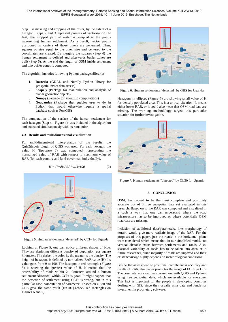
Figure 6. Human settlements "detected" by GHS for Uganda

Hexagons in ellipses (Figure 5) are showing small value of H

for densely populated area. This is a critical situation. It means

either lower RAR, or it could also mean that OSM road data are

missing. The working methodology targets this particular

situation for further investigation.

Figure 7. Human settlements "detected" by GL30 for Uganda

5. CONCLUSION

OSM, has proved to be the most complete and positinaly

accurate out of 3 free geospatial data set evaluated in this

research. Based on it, the RAR was computed and visualized in

a such a way that one can understand where the road

infrastructure has to be improved or where potentially OSM

road data are missing.

Inclusion of additional data/parameters, like morphology of

terrain, would give more realistic image of the RAR. For the

purposes of this paper, just the roads in the horizontal plane

were considered which means that, in our simplified model, no

vertical obstacle exists between settlements and roads. Also,

seasonal variability of roads has to be taken into account in

future researches, since majority of roads are unpaved and their

existence/usage highly depends on meteorological conditions.

Beside the assessment of positional/completeness accuracy and

results of RAR, this paper promotes the usage of FOSS in GIS.

The complete workload was carried out with QGIS and Python,

using free geospatial data, which are available for everyone.

This fact is important for the people in developing countries

dealing with GIS, since they usually miss data and funds for

investment in proprietary software.



1571

ACKNOWLEDGEMENTS

Special thanks to Andre Nonguierma and Girum Asrat

(UNECA) for providing us data. Many thanks also to other data

providers: OSM, ESA, NGCC, EC and CIESIN.

6. REFERENCE

Antenucci, J., Brown K., Croswell P., Kevany, M., Archer, H.,

1991. Geographic Information Systems: A guide to the

technology. Springer, New York, US. 102-103.

Brovelli, M.A., Minghini, M., Molinari, M., Mooney, P., 2015.

A FOSS4G-based procedure to compare OpenStreetMap and

authoritative road network datasets. Geomatics Workbooks 12,

235-238, ISSN 1591-092X.

Brovelli, M. A., Minghini, M. , Molinari, M. and Mooney, P.,

2017, Towards an automated comparison of OpenStreetMap

with authoritative road datasets. Transactions in GIS, 21: 191-

206. doi:10.1111/tgis.12182

CEN, 1995, TC 287 N369: Geographic information - Data

description - Quality. Technical report, European Committee

for Standardization, Working Draft at stage 32, London, UK.

Goodchild, M. F., 2007. Citizens as sensors: the world of

volunteered Geography. GeoJournal. 69, 211-221.

doi.org/10.1007/s10708-007-9111-y.

Haklay, M., 2010. how good is volunteered geographical

information? A comparative study of OpenStreetMap and

ordnance survey datasets. Environment and Planning B:

Planning and Design, 37(4), 682–703.

https://doi.org/10.1068/b35097

Ivanova, E. and Masarova, J., 2013. Importance of road

infrastructure in the economic development and

competitiveness, Economics and Management,

doi.org/10.5755/j01.em.18.2.4253.

Leitner, M. and Arsanjani, J.J., 2017. citizen empowered

mapping, Springer Publishing Company, 188-200,

http://dx.doi.org/10.1007/978-3-319-51629-5.

Ludwig, I., Voss, A., Krause-Traudes, M., 2011. Comparison of

the street networks of Navteq and OSM in Germany, Advancing

Geoinformation science of a changing world, Springer Berlin

Heidelberg, 65–84, http://dx.doi.org/10.1007/978-3-642-19789-

5_4.

Martinez-Llario, J., Coll, E., Arteaga, D., 2009. Road data

analisys with FOSS GIS. Proceedings of the 9th WSEAS

International Conference on Applied Computer Science, 191-

194, ISSN 1790-5109.

Mooney, P. and Corcoran, P., 2014. Analysis of interaction and

co‐editing patterns amongst OpenStreetMap contributors.

Transactions in GIS 18, 633–59,

https://doi.org/10.1111/tgis.12051.

Moreira de Sousa, L. and Leitão, J. P., 2017. HexASCII: A file

format for cartographical hexagonal rasters. Transactions in

GIS. 10.1111/tgis.12304.

Neis, P. and Zipf, A., 2012. Analyzing the contributor activity

of a volunteered geographic information project — The case of

OpenStreetMap. ISPRS International Journal of Geo-

Information. 1. 146-165. 10.3390/ijgi1020146.

Siebritz, L., Sithole, G., 2014. Assessing the accuracy of

OpenStreetMap data in South Africa for the purpose of

integrating it with authoritative data. PhD Thesis, University of

Cape Town, SA.

https://pdfs.semanticscholar.org/2a9c/c10127fb5546269e77aed

6afe71df5235956.pdf.

Nkomo, S. L., Desai, S., & Peerbhay, K. 2016. Assessing the

conditions of rural road networks in South Africa using visual

observations and field-based manual measurements: A case

study of four rural communities in Kwa-Zulu Natal. Review of

Social Sciences, 1(2), 42-55.

doi:http://dx.doi.org/10.18533/rss.v1i2.24

Vincent, S., Civil Design Solutions, 2018. status review of the

updated Rural Access Index (RAI), Draft Final Report,

GEN2033C. London: ReCAP for DFID. http://research4cap.org/Library/Vincent-CDS-2018-

StatusReviewUpdatedRAI-FinalReport_GEN2033C-

180529.pdf

Zielstra, Dennis & Hochmair, Hartwig. 2011. Comparative

study of pedestrian accessibility to transit stations using free and

proprietary network data. Journal of the Transportation

Research Board. 2217. 10.3141/2217-18.



1572



http://dx.doi.org/10.1007/978-3-642-19789-5_4

http://dx.doi.org/10.1007/978-3-642-19789-5_4

https://doi.org/10.1111/tgis.12051.

https://onlinelibrary.wiley.com/action/doSearch?ContribAuthorStored=de+Sousa%2C+Lu%C3%ADs+Moreira

https://onlinelibrary.wiley.com/action/doSearch?ContribAuthorStored=Leit%C3%A3o%2C+Jo%C3%A3o+Paulo

Documents

ANALYSIS OF FREE ROAD DATA IN TANZANIA, …...ANALYSIS OF FREE ROAD DATA IN TANZANIA, UGANDA AND KENYA USING FREE AND OPEN SOURCE SOFTWARE Stefan Jovanovic 1, Dina Jovanovic 1, Gorica