Analysis of fracture in thin shells by overlapping paired ... · Analysis of fracture in thin shells by overlapping paired elements Pedro M.A. Areias, J.H. Song, Ted Belytschko *

$Page 1: Analysis of fracture in thin shells by overlapping paired ... · Analysis of fracture in thin shells by overlapping paired elements Pedro M.A. Areias, J.H. Song, Ted Belytschko *$
www.elsevier.com/locate/cma

Comput. Methods Appl. Mech. Engrg. 195 (2006) 5343–5360

Analysis of fracture in thin shells by overlapping paired elements

Pedro M.A. Areias, J.H. Song, Ted Belytschko *

Department of Mechanical Engineering, Northwestern University, 2145 Sheridan Road, Evanston, IL 60208-3111, USA

Received 18 April 2005; received in revised form 12 October 2005; accepted 14 October 2005

Abstract

A finite element methodology for evolution of cracks in thin shells using mid-surface displacement and director field discontinuities ispresented. We enrich the mid-surface displacement and director fields of a discrete Kirchhoff–Love quadrilateral element using a piece-wise decomposition of element kinematics, which leads to a basis that is a variant of the one used in the extended finite element method.This allows considerable simplifications in the inclusion of the shell director field. A cohesive law is employed to represent the progressiverelease of the fracture energy. In contrast with previous works, we retain the original quadrature points after the formation of a crack,which, in combination with an elasto-plastic multiplicative decomposition of the deformation gradient, avoids the previously requiredinternal variable mapping during crack evolution. Results are presented for large strain elastic and elasto-plastic crack propagation.� 2005 Elsevier B.V. All rights reserved.

Keywords: Fracture; Elasto-plasticity; Shell elements; Extended finite element method

1. Introduction

Argyris’ study of large rotations [1] has had a profound impact on finite element methods for large displacements ofshells. It provided a consistent framework for treating large deformation of shells and beams and influenced later worksuch as Simo et al. [2,3] and Ramm and co-workers [4–6]. In this paper we describe a Kirchhoff–Love shell element forarbitrary crack propagation that employs large rotations about moving axis. This work is motivated by a previous methodwe developed for fracture in plate and shell structures using the extended finite element method (XFEM) [7]. Two difficul-ties became apparent during the course of that work. One was the relatively non-trivial incorporation of the director fieldenrichment. Another was the difficulty in formulating a cohesive law with transverse shear stress components. Here wedescribe a discrete Kirchhoff–Love element (see also [8]), for crack propagation. We use a reinterpretation of the XFEMmethodology which leads to a formulation similar to the Hansbo and Hansbo [9] approach to discontinuities (see also [10]).The introduction of a displacement discontinuity in a discrete Kirchhoff–Love element is surprisingly straightforward usingthis technique. With a number of proposed considerations, it is possible to add crack propagation to an existing finite ele-ment code with minimal modifications. Very little has been done on arbitrary progressive fracture in plates and shells. Dol-bow et al. [11] considered non-propagating cracks in plates by XFEM. An inter-element cracking formulation for shellswas recently proposed by Cirak et al. [12] using cohesive elements, in the explicit dynamics context. Lee et al. [13] employedcommercial codes and element deactivation to model circular fracture in punched plates.

We describe some details of this shell finite element and provide a more general formulation of the fracture model. Theelasto-plastic framework adopted is based on Lee’s [14] multiplicative decomposition of the deformation gradient and anunsymmetric return mapping algorithm, proposed here (see also [15]).

0045-7825/$ - see front matter � 2005 Elsevier B.V. All rights reserved.

doi:10.1016/j.cma.2005.10.024

* Corresponding author. Tel.: +1 847 491 4029; fax: +1 847 491 4011.E-mail address: [email protected] (T. Belytschko).

mailto:[email protected]

5344 P.M.A. Areias et al. / Comput. Methods Appl. Mech. Engrg. 195 (2006) 5343–5360

The paper is organized as follows. In Section 2 we describe the shell model and the proposed enrichment. In Section 3 wepresent the elasto-plastic algorithm employed in the analysis and in Section 4 we succinctly present the particular cohesivemechanism employed. In Section 5 we present some numerical examples, including an example of plate tearing and a pres-surized cylinder. Finally we draw some conclusions in Section 6.

2. Shell model and enriched discretization

Recently, we proposed a fully nonlinear quadrilateral shell element based on discrete Kirchhoff–Love conditions [8]. Thepurpose of that work was to extend the range of application of our [7] shell fracture model to folded and/or kinked shells.We here apply the model in [8] to fracture of thin plates and shells. The element degrees of freedom are mid-side rotationsand corner-node displacements. Local duplication of homologous degrees of freedom is used in the present enrichment,which is similar to what is carried out in XFEM derivations (e.g. [16–18]). This method is motivated by the Hansboand Hansbo technique [9]. Although we develop the cracking formulation for a particular element here, the formulationis more generally applicable to elements whose deformation is described by mid-surface displacements and directors.

This displacement enrichment can be viewed as an independent interpolation of the displacement field for both sides of acracked finite element. It can be shown that this enrichment is, in essence, the same as the original XFEM enrichment, butit allows further insight into the interpretation, and in particular a new perspective on the director field interpolation. Themethodology has the following noteworthy aspects:

• The Kirchhoff–Love (KL) constraints (c.f. [19]) are satisfied in both parts of a cracked element.• It is possible to view the piecewise enrichment as a superposition of two elements, with modified quadrature weights to

account for the corresponding effective areas. This facilitates the task of introducing cracks in existing elements withoutexplicitly considering the discontinuity in the displacement field.

• Exact shell kinematics are preserved and minimum changes to our shell element are required.• Curvilinear coordinates are employed in the equilibrium equations.• Large strain plasticity is dealt within the framework of the plastic metric. Pade approximations are employed for the

exponential and logarithmic functions of an unsymmetric tensor. This removes the necessity of using variable transferbetween the pristine and cracked elements.

We consider a cracked shell as a domain (or region) in E3 (the Euclidean 3-space), whose undeformed and unstressedconfiguration is X0. A point belonging to the shell is identified by its position in X0, denoted as X. We assume that X0

is partitioned into two sub-domains Xþ0 and X�0 : X0 ¼ Xþ0 [ X�0 and we use the corresponding notation for X, withXþ 2 Xþ0 and X� 2 X�0 . We define a function which indicates if a given point X belongs to X�0 or Xþ0 according to its sign.This function f(X) is such that f(X) = 0 is the implicit equation of the crack surface and f(X�) < 0 and f(X+) > 0. Fig. 1

Fig. 1. Partition of the reference configuration into two sub-domains of a shell containing one crack. Any deformed configuration can be obtained fromthe deformation map defined in the corresponding undeformed sub-domain.

P.M.A. Areias et al. / Comput. Methods Appl. Mech. Engrg. 195 (2006) 5343–5360 5345

shows these sub-domains, along with two parts of the crack surface corresponding to the constrained (C0a) and uncon-strained (C0b) crack surface. The crack surface partition is defined as C0 = C0a [ C0b with C0a \ C0b = ;. According tothe sub-domain, we consider two distinct deformation maps u� : X�0 3 X� 7! x� 2 X� and uþ : Xþ0 3 Xþ 7! xþ 2 Xþ

and the additional condition: X 2 C0a) u+(X) � u�(X). In the sub-domain C0b the deformation maps can assume distinctvalues. With the graphical representation of Fig. 1 we can interpret the crack as the part of C for which u+ k u�. We candefine Ca = u(C0a) and, for C0b, Cþb ¼ uþðC0bÞ and C�b ¼ u�ðC0bÞ. In other words, a cracked configuration can be viewed astwo pristine configurations with a common domain (denoted here as Ca).

One can observe that, in terms of kinematics, no substantial difference exists between a cracked body and an un-crackedone. It is also noteworthy that when a discretization is carried out, unless the crack path is known a priori, the crack pathCb would not coincide with finite elements edges. To deal with this fact, we use the following procedure. For each elementcontaining a given part of C0b, which we will denote as PðC0bÞ, we use a superposition of two elements with common partsin X+ and X�, but one associated with the deformation map u+ and the other one associated with u�. Although this inter-pretation by itself is not new (see, e.g. [9]), it naturally allows a formulation of cracked rods and shells with distinct directorfields (n+ and n� in Fig. 1) circumventing the association of these with an underlying (un-cracked) shell as was done in ourprevious work [8].

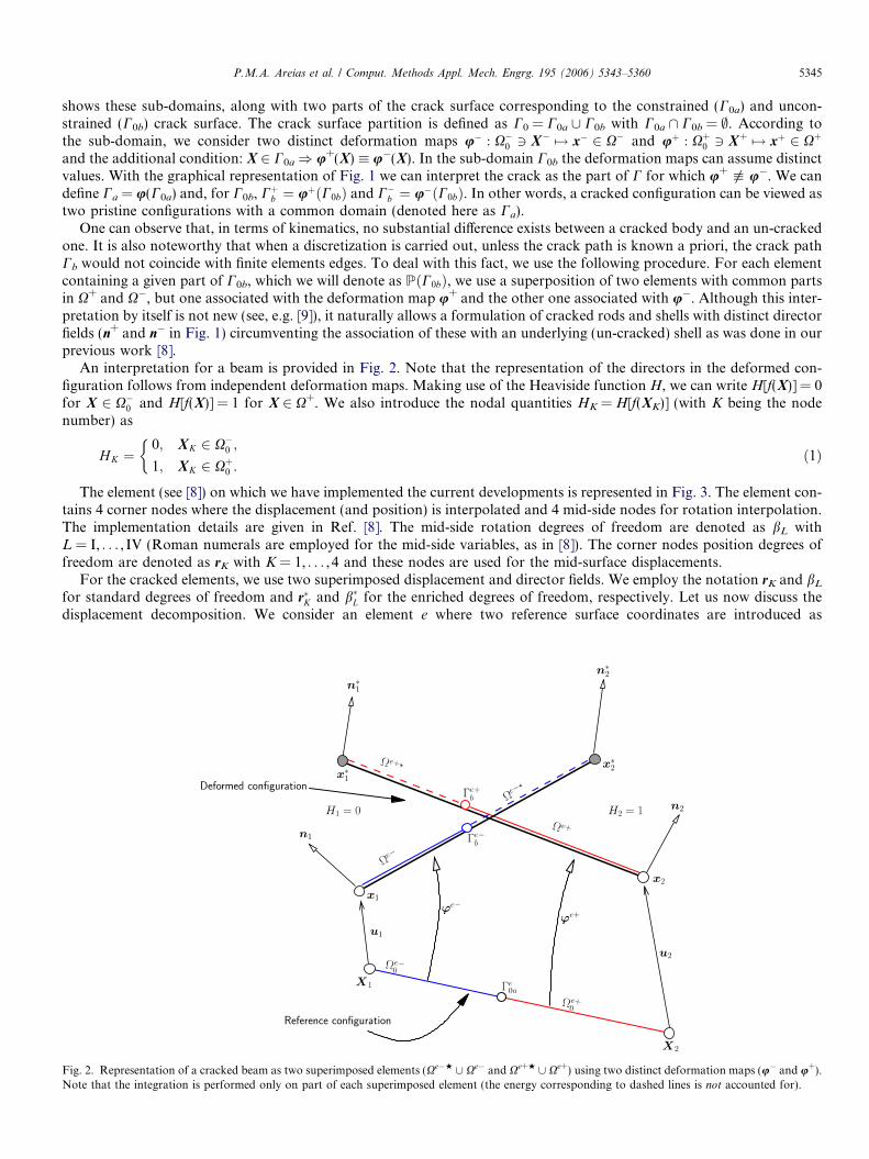
An interpretation for a beam is provided in Fig. 2. Note that the representation of the directors in the deformed con-figuration follows from independent deformation maps. Making use of the Heaviside function H, we can write H[f(X)] = 0for X 2 X�0 and H[f(X)] = 1 for X 2 X+. We also introduce the nodal quantities HK = H[f(XK)] (with K being the nodenumber) as

H K ¼0; XK 2 X�0 ;

1; XK 2 Xþ0 .

�ð1Þ

The element (see [8]) on which we have implemented the current developments is represented in Fig. 3. The element con-tains 4 corner nodes where the displacement (and position) is interpolated and 4 mid-side nodes for rotation interpolation.The implementation details are given in Ref. [8]. The mid-side rotation degrees of freedom are denoted as bL withL = I, . . . , IV (Roman numerals are employed for the mid-side variables, as in [8]). The corner nodes position degrees offreedom are denoted as rK with K = 1, . . . , 4 and these nodes are used for the mid-surface displacements.

For the cracked elements, we use two superimposed displacement and director fields. We employ the notation rK and bL

for standard degrees of freedom and r�K and b�L for the enriched degrees of freedom, respectively. Let us now discuss thedisplacement decomposition. We consider an element e where two reference surface coordinates are introduced as

Fig. 2. Representation of a cracked beam as two superimposed elements (Xe�w [ Xe� and Xe+w [ Xe+) using two distinct deformation maps (u� and u+).Note that the integration is performed only on part of each superimposed element (the energy corresponding to dashed lines is not accounted for).

Fig. 3. Shell element based on discrete Kirchhoff–Love conditions. Directors (nI is represented) are interpolated at the mid-sides. For simplicity only therotation of side I is shown.


h = {h1,h2} such that h 2 [�1,1]2 and a third coordinate identified as the signed distance to the reference surface, h3. Usingthe notation r+ and r� for the mid-surface positions of the shell element in each of the parts Xe� [ Xe�w and Xe+ [ Xe+w,respectively, we can write r as

r ¼

X4

K¼1ð1� H KÞNKðhÞrK þ

X4

K¼1H KN KðhÞr�K|fflfflfflfflfflfflfflfflfflfflfflfflfflfflfflfflfflfflfflfflfflfflfflfflfflfflfflfflfflfflfflfflfflfflfflfflfflfflfflfflfflffl{zfflfflfflfflfflfflfflfflfflfflfflfflfflfflfflfflfflfflfflfflfflfflfflfflfflfflfflfflfflfflfflfflfflfflfflfflfflfflfflfflfflffl}

rþ

; f ðXÞ > 0;

X4

K¼1HKN KðhÞrK þ

X4

K¼1ð1� HKÞN KðhÞr�K|fflfflfflfflfflfflfflfflfflfflfflfflfflfflfflfflfflfflfflfflfflfflfflfflfflfflfflfflfflfflfflfflfflfflfflfflfflfflfflfflfflffl{zfflfflfflfflfflfflfflfflfflfflfflfflfflfflfflfflfflfflfflfflfflfflfflfflfflfflfflfflfflfflfflfflfflfflfflfflfflfflfflfflfflffl}

r�

; f ðXÞ < 0;

8>>>>><>>>>>:

ð2Þ

where K is the corner node number for Xe and NK(h) represents the bilinear shape function of corner node K. For the spa-tial directors, the same type of interpolation follows, where use is made of two directors n+ and n�:

n ¼

XIV

L¼Ið1� H LÞMLðhÞnL þ

XIV

L¼IHLMLðhÞn�L|fflfflfflfflfflfflfflfflfflfflfflfflfflfflfflfflfflfflfflfflfflfflfflfflfflfflfflfflfflfflfflfflfflfflfflfflfflfflfflffl{zfflfflfflfflfflfflfflfflfflfflfflfflfflfflfflfflfflfflfflfflfflfflfflfflfflfflfflfflfflfflfflfflfflfflfflfflfflfflfflffl}

nþ

; f ðXÞ > 0;

XIV

L¼IH LMKðhÞnL þ

X4

L¼1ð1� H LÞMLðhÞn�L|fflfflfflfflfflfflfflfflfflfflfflfflfflfflfflfflfflfflfflfflfflfflfflfflfflfflfflfflfflfflfflfflfflfflfflfflfflfflfflfflffl{zfflfflfflfflfflfflfflfflfflfflfflfflfflfflfflfflfflfflfflfflfflfflfflfflfflfflfflfflfflfflfflfflfflfflfflfflfflfflfflfflffl}

n�

; f ðXÞ < 0;

8>>>>><>>>>>:

ð3Þ

with L being the mid-side node number (L = I, . . . , IV) and ML(h) represents the mid-side shape function corresponding tonode L. The shape functions ML(h) are given by (see also [8]):

MLðh1; h2Þ ¼ 1

4þ 3

8ðh2LÞ2½ðh2Þ2 � ðh1Þ2� þ 1

2h2Lh2 þ 3

8ðh1LÞ2½ðh1Þ2 � ðh2Þ2� þ 1

2h1Lh1. ð4Þ

Note that, despite the apparent simplicity of the relations (2), the nodal directors nL and n�L are functions of both r and r* in(2), because of the Kirchhoff–Love conditions as will become apparent later. Using the decompositions (2), the position ofa given point X can be presented as a function of the sub-domain to which it belongs:

x � uðXÞ ¼

rþðhÞ þ h3nþðhÞ|fflfflfflfflfflfflfflfflfflfflfflffl{zfflfflfflfflfflfflfflfflfflfflfflffl}xþ

; f ðXÞ > 0;

r�ðhÞ þ h3n�ðhÞ|fflfflfflfflfflfflfflfflfflfflfflffl{zfflfflfflfflfflfflfflfflfflfflfflffl}x�

; f ðXÞ < 0.

8>>><>>>:

ð5Þ

In the following, we use the notation (•),a to denote derivatives with respect to ha, a = 1,2 and analogously (•),i for hi;i = 1,2,3 with (•) being an arbitrary quantity.

Let sij represent the contravariant components of the Kirchhoff stress tensor (in the basis x,a � x,b) which are also thecomponents of the second Piola–Kirchhoff stress tensor in the basis X,a � X,b. Then the weak form of equilibrium can bewritten, using a parent domain volume Ve = [�1,1]2 · [�h/2,h/2] for each element, and using

ffiffiffiffiGp¼ X ;1 � ðX ;2 � X ;3Þ, as


XNe

e¼1

ZV e

sabx;b � dx;affiffiffiffiGp

dh1 dh2 dh3 ¼ dW E; ð6Þ

where dWE is the virtual work performed by the external loading and cohesive forces (given in Section 4). The derivatives(•),a follow from the derivatives of the shape functions NK(h) and ML(h), denoted as NK;a ¼ oNK

oha and ML;a ¼ oMLoha . The upper

limit Ne is the total number of elements in a particular discretization.Our formulation is based on the covariant components of the Cauchy–Green deformation tensor. If the covariant com-

ponents of the material metric tensor are introduced as

Gij ¼ X ;i � X ;j; ð7Þthen the contravariant components of the material metric tensor are given by [Gij] = [Gij]

�1 and the Cauchy–Green tensor isobtained using the contravariant basis vectors Gi = GijX, j:

C ¼ x;i � x;j|fflfflffl{zfflfflffl}Cij

G i � G j. ð8Þ

The Kirchhoff–Love conditions are imposed to C as

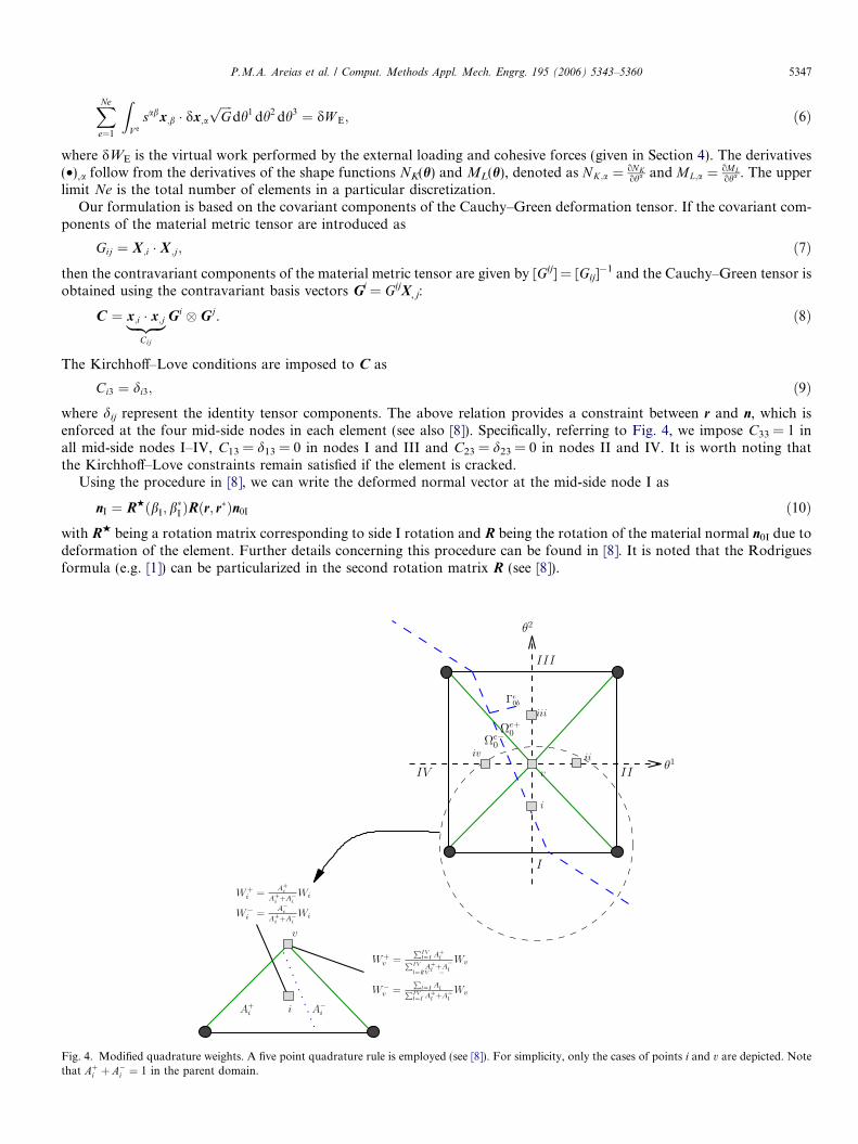
Ci3 ¼ di3; ð9Þwhere dij represent the identity tensor components. The above relation provides a constraint between r and n, which isenforced at the four mid-side nodes in each element (see also [8]). Specifically, referring to Fig. 4, we impose C33 = 1 inall mid-side nodes I–IV, C13 = d13 = 0 in nodes I and III and C23 = d23 = 0 in nodes II and IV. It is worth noting thatthe Kirchhoff–Love constraints remain satisfied if the element is cracked.

Using the procedure in [8], we can write the deformed normal vector at the mid-side node I as

nI ¼ RHðbI; b�I ÞRðr; r�Þn0I ð10Þ

with Rw being a rotation matrix corresponding to side I rotation and R being the rotation of the material normal n0I due todeformation of the element. Further details concerning this procedure can be found in [8]. It is noted that the Rodriguesformula (e.g. [1]) can be particularized in the second rotation matrix R (see [8]).

Fig. 4. Modified quadrature weights. A five point quadrature rule is employed (see [8]). For simplicity, only the cases of points i and v are depicted. Notethat Aþi þ A�i ¼ 1 in the parent domain.


The first variation of x,b; dx,b, can be written, according to the corresponding sub-domain, as

dxþ;a ¼X4

K¼1

ð1� H KÞN K;adrK þX4

K¼1

HKNK;adr�K þXIV

L¼I

ð1� HLÞMLðhÞdnLðdxk; dx�k ; dblÞ þXIV

L¼I

H LMLðhÞdn�Lðdxk; dx�k ; db�l Þ;

ð11aÞ

dx�;a ¼X4

K¼1

H KNK;adrK þX4

K¼1

ð1� H KÞNK;adr�K þXIV

L¼I

H LMLðhÞdnLðdxk; dx�k ; dblÞ þXIV

L¼I

ð1� H LÞMLðhÞdn�Lðdxk; dx�k ; db�l Þ;

ð11bÞ

where the explicit dependence of nL and n�L on xk, x�k , bl and b�l is apparent, with k = 1, . . . , 4 and l = I, . . . , IV (note the useof lower case subscripts for these arguments).

The modified quadrature weights are represented in Fig. 4 and are calculated in the mid-surface parent domainh 2 [�1,1]2. We scale the weights so that the correct areas for each of the parts Xþe and X�e is obtained.

The first variation of dWI, which is required for the calculation of the tangent matrix, is given by

ddW I ¼XNe

e¼1

ZV e

sab½ðdr;a þ h3dn;aÞ � ðdr;b þ h3dn;bÞ þ ðr;a þ h3n;aÞ � ðddr;b þ h3ddn;bÞ��

þ 2Cabcg½ðr;a þ h3n;aÞ � ðdr;b þ h3dn;bÞ�½ðr;c þ h3n;cÞ � ðdr;g þ h3dn;gÞ� þ dsa3ðdn � r;a þ n � dr;aÞþ dsa3ðdn � r;a þ n � dr;aÞ þ sa3ðddn � r;a þ dn � dr;aÞ þ sa3ðdn � dr;a þ n � ddr;aÞ

� ffiffiffiffiGp

dh1 dh2 dh3 ð12Þ

with Cabcg representing the contravariant components of the consistent modulus, to be introduced in the following section.The tangent stiffness matrix obtained from (12) is generally unsymmetric in the elasto-plastic case.

The interpretation as a XFEM element can be carried out very simply if we introduce the nodal sign as sK = 2HK � 1and write the displacement as u = Hu+ + (1 � H)u� with H denoting the step function. Then, it is possible to show that thetraditional XFEM degrees of freedom are obtained by linear combination of the present method degrees of freedom. Theproof has been given in [20].

3. Elastic–plastic algorithm

In our previous work [8], we used the contravariant components of the Kirchhoff stress tensor to establish the weak formof equilibrium equations for the shell model. To take advantage of the simplicity of our previous derivations, we retain thecurvilinear coordinates in the inelastic range.

With that purpose, we use the large strain elasto-plastic formulation by Miehe [21] particularized for a Kirchhoff–Loveshell model. In contrast with that work, we do not use a spectral decomposition of the Cauchy–Green tensor and opt to usePade interpolants (see also [22] and [15]). Note that this corresponds to the dual formulation of elasto-plasticity [23] (instress space) and is now a common procedure in many applications. For this reason, and because we are confined to iso-

tropic constitutive laws, we only present the main results. The formulation follows the multiplicative decomposition of thedeformation gradient F, as in Lee [14], and employed with success in the seminal work of Simo and Ortiz [24]:

F ¼ FeFp. ð13ÞWe define the right Cauchy–Green tensors (elastic and plastic) accordingly

C e ¼ FeT

Fe;

Cp ¼ FpT

Fp.

Note that Cp is also called the covariant plastic metric.With this notation, we can introduce a generally unsymmetric tensor CE such as

C ¼ CECp. ð14ÞThe elasto-plastic formulation based on decomposition (14) circumvents the explicit evolution for the plastic spin (and alsothe non-uniqueness aspect of Lee’s decomposition (13)). C E can be written as a function of C e according to

CE ¼ Fp�1

C eFp. ð15ÞThe formulation does not rely on the explicit identification of F e or F p and these quantities remain undetermined. Mak-

ing use of a spectral decomposition of C e and relating it to C E, we make further progress by identifying that they possessanalogous forms:


C e ¼ NENT; ð16Þwith N being a matrix containing, columnwise, the unitary eigenvectors of Ce and E ¼ diag½k2

i � where ki are the princi-pal elastic stretches. Due to orthogonality of the eigenvectors, NT = N�1. Inserting (16) into (15), we obtain

CE ¼ ðFpT

NÞEðFpT

NÞ�1. ð17ÞIf we introduce NE ¼ FpT

N then it is clear that C p can be expressed as

Cp ¼ NENET

. ð18ÞA more concise decomposition of C E is obtained, identifying N E as the matrix of right eigenvectors of C E:

CE ¼ NEENE�1

. ð19ÞAfter decomposing C E according to (19), we can normalize the eigenvectors with Eq. (18).Using (19), we can write the spectral decomposition of C, as a counterpart of (16), keeping in mind that NE is not gen-

erally composed of unitary vectors (as is N):

C ¼ NEENET

. ð20ÞThese direct derivations are, however, purposeless if C p is obtained directly from F p (i.e. if F p is considered to be an

historical variable). Let us introduce an isotropic strain energy density as a function of the state variables C, which is ameasure of total strain, C p which is a measure of plastic strain, and n which represents the set of remaining internal vari-ables of state. The set {C p,n} constitutes the internal variables. We use the usual notation w for the strain energy function:

w � wðC ;Cp; nÞ. ð21ÞThe evolution laws of both Cp and n are derived as to comply, ab initio, with the second law of thermodynamics, which

can be written in the form of the Clausius–Planck inequality, in the absence of thermal terms

Dint ¼1

2S : _C � _w P 0; ð22Þ

where Dint is the internal dissipation term. Inserting the time-derivative of (21) into (22) it is possible to write

Dint ¼1

2S � ow

oC

� �: _C � Sp : _Cp � v : _n P 0; ð23Þ

where Sp ¼ owoCp and v ¼ ow

on. Using the fact that, in the absence of plastic evolution and ‘‘frozen’’ internal variable evolution

(i.e. _n ¼ 0) the constitutive law should still satisfy (23) and the accompanying process is non-dissipative ðDint ¼ 0Þ, we areable to write S ¼ 2 ow

oCfor this condition to hold for arbitrary _C . Of course, if one of the previous conditions for the internal

variable evolution does not hold, it is possible to have a distinct value for S, but this situation is not considered in our work(see also [25]). Note that _Cp ¼ 0 does not generally imply that _n ¼ 0, but this is assumed to hold. The evolution laws areobtained from a ‘‘potential’’ of dissipation, which is denoted as

F �FðCp; n; Sp; vÞ ð24Þfrom which we postulate that

_Cp ¼ _aoF

oSp ;

_n ¼ _aoF

ov;

where _a P 0 is a plastic parameter (also called plastic multiplier in the associative case).Let us introduce the elastic part of the strain energy function (the strain energy function can be decomposed into elastic

and plastic parts, e.g. [23]) as a function of the principal elastic stretches: we � we(ki) with i = 1,2,3. If we introduce theprincipal elastic Hencky strain components as ei = lnki, and the principal Kirchhoff stress components as si ¼ owe

oei, it is pos-

sible to express, under coaxiality conditions, the second Piola–Kirchhoff stress tensor as

S ¼ NE�T

SDNE�1 ¼ sabX ;a � X ;b; ð25Þwith SD ¼ diag½si

k2i�. A conjugate force to the plastic metric C p is S p, the plastic force, which can be written as

Sp ¼ owe

oCp ¼1

2Cp�1

CS; ð26Þ


where use was made of the chain rule and symmetry of C p, C and S and the symmetry of the result:

owoCp ¼

owoC

:oC

oCp ¼1

2SCE ¼ 1

2CET

S. ð27Þ

The term CS in (26) is the so-called mixed-variant stress tensor [21,25], and is here denoted as R. This tensor is generallyunsymmetric.

Finally, the flow law can be written as

_Cp ¼ 2 _aoF

oRCp ð28Þ

and the elastic law is given by

R ¼ j tr eI þ ldev e; ð29Þwith

2e ¼ ln CE.

Let us now integrate the flow law (28) using the exponential mapping, by introducing two time steps tn and tn+1, a timeincrement denoted Dt = tn+1 � tn, and the variation of the plastic multiplier between these two instants (Da):

CEnþ1 ¼ CE

nHexp �2Da

oF

oR

; ð30Þ

where CEnH

is given by

CEnH¼ Cnþ1Cp�1

n ð31Þor, making use of the notation en+1 and enw:

enþ1 ¼ enH � DaoF

oR. ð32Þ

Note that the finite strain consistent modulus can be written as a function of a ‘‘small strain’’ modulus C using indicialnotation:

Cijkl ¼oSij

oCkl¼ C�1

ir Crjpqoepq

oCEkv

Cp�1

lv � C�1ik C�1

lr Rrj. ð33Þ

With (33) we can write the classical relation between the second Piola–Kirchhoff stress and the Green–Lagrange strainE2 ¼ 1

2C � 1

2I as _S ¼ 2C : _E2.

The small strain analogy of (32) allows us to use a small strain elasto-plastic code, adequately modified to deal withunsymmetric stress and strain tensors. It is interesting to note that approximations to logarithms and exponentials canbe employed, as these are found to be sufficient in metal plasticity, even for considerably large strains [22,15]. The algo-rithm in Table 1 shows the adopted procedure. We use first order approximations for the exponential and second orderfor the logarithm functions:

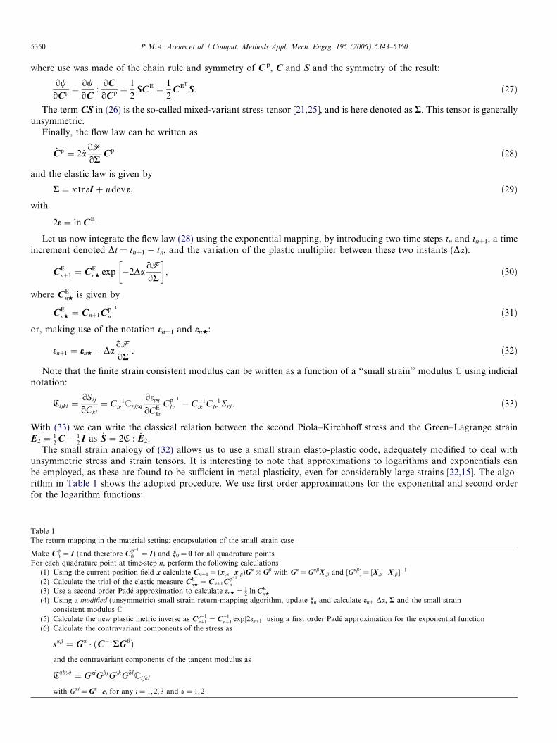
Table 1The return mapping in the material setting; encapsulation of the small strain case

Make Cp0 ¼ I (and therefore Cp�1

0 ¼ I) and n0 = 0 for all quadrature pointsFor each quadrature point at time-step n, perform the following calculations

(1) Using the current position field x calculate Cn+1 = (x,a Æ x,b)Ga � Gb with Ga = GabX,b and [Gab] = [X,a Æ X,b]�1

(2) Calculate the trial of the elastic measure CEnH¼ Cnþ1Cp�1

n

(3) Use a second order Pade approximation to calculate enH ¼ 12

ln CEnH

(4) Using a modified (unsymmetric) small strain return-mapping algorithm, update nn and calculate en+1Da, R and the small strainconsistent modulus C

(5) Calculate the new plastic metric inverse as Cp�1nþ1 ¼ C�1

nþ1 exp½2enþ1� using a first order Pade approximation for the exponential function(6) Calculate the contravariant components of the stress as

sab ¼ Ga � ðC�1RGbÞand the contravariant components of the tangent modulus as

Cabcd ¼ GaiGbjGckGdlCijkl

with Gai = Ga Æ ei for any i = 1,2,3 and a = 1,2


e ffi e1 ¼ e0 I � 1

3e0e0

� ��1

; ð34aÞ

with

e0 ¼ ðCE � IÞðCE þ IÞ�1 ð34bÞand

CE ffi ðI � eÞ�1ðI þ eÞ. ð34cÞThe derivative

oepq

oCEkv

in (33) can use the first Pade approximation (34c) as the final C E is employed, which for metal plas-

ticity is sufficiently close to the unitary matrix [22,15]. In this case

oepq

oCEkv

ffioe0

pq

oCEkv

¼ ðdpk � e0pkÞðI þ CEÞ�1

vq .

The reason for using distinct orders of approximation in (34a) and (34c) is that the trial elastic strains can be substan-tially larger than the corrected elastic strains in metal plasticity.

In our present application, we employ J2 associative plasticity, where the dissipation potential F coincides with the yieldfunction (see also [25]).

4. Cohesive law

We make use of a combination of a stability criterion (as a fracture indicator) and maximum principal strains (to predictthe crack path) which was found to be convenient for fracture initiation and propagation [26]. For a KL constrained med-ium, the stability condition should take into account the KL constraints and the compatibility conditions (resulting in a setof non-simple constraints see, e.g. [19]).

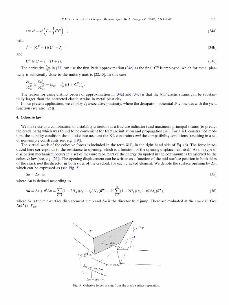
The virtual work of the cohesive forces is included in the term dWE in the right hand side of Eq. (6). The force intro-duced here corresponds to the resistance to opening, which is a function of the opening displacement itself. As this type ofdissipation mechanism occurs in a set of measure zero, part of the energy dissipated in the continuum is transferred to thecohesive law (see, e.g. [26]). The opening displacement can be written as a function of the mid-surface position in both sidesof the crack and the director in both sides of the cracked, for each cracked element. We denote the surface opening by Du,which can be expressed as (see Fig. 5):

Du ¼ Du �m; ð35Þwhere Du is defined according to

Du ¼ Drþ h3Dn ¼X4

K¼1

ð1� 2HKÞðrK � r�KÞNKðhHÞ þ h3XIV

L¼I

ð1� 2HLÞðnL � n�LÞMLðhHÞ; ð36Þ

where Dr is the mid-surface displacement jump and Dn is the director field jump. These are evaluated at the crack surfaceX(hw) 2 C0b.

Fig. 5. Cohesive forces arising from the crack surface separation.


If we denote the part of dWE corresponding to the cohesive virtual work as dW cE, then we can write it using the Kirchhoff

stress value rn as

dW cE ¼ �

ZCOb

rndDudA ¼ �Z

COb

rn � dDudA; ð37Þ

where A represents the area of Ce0b.

The first variation of dW cE is required for the application of the Newton method. It can be written as

ddW cE ¼ �

ZCOb

dDuTKdDudA; ð38Þ

with

K ¼ orn

oDum�m. ð39Þ

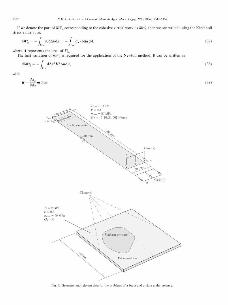
Fig. 6. Geometry and relevant data for the problems of a beam and a plate under pressure.


In the studies reported here, the particular constitutive model for the cohesive zone is given by (see also [27]):

rn ¼rmax

�exp � rmax

Gf

�

� �Du; ð40Þ

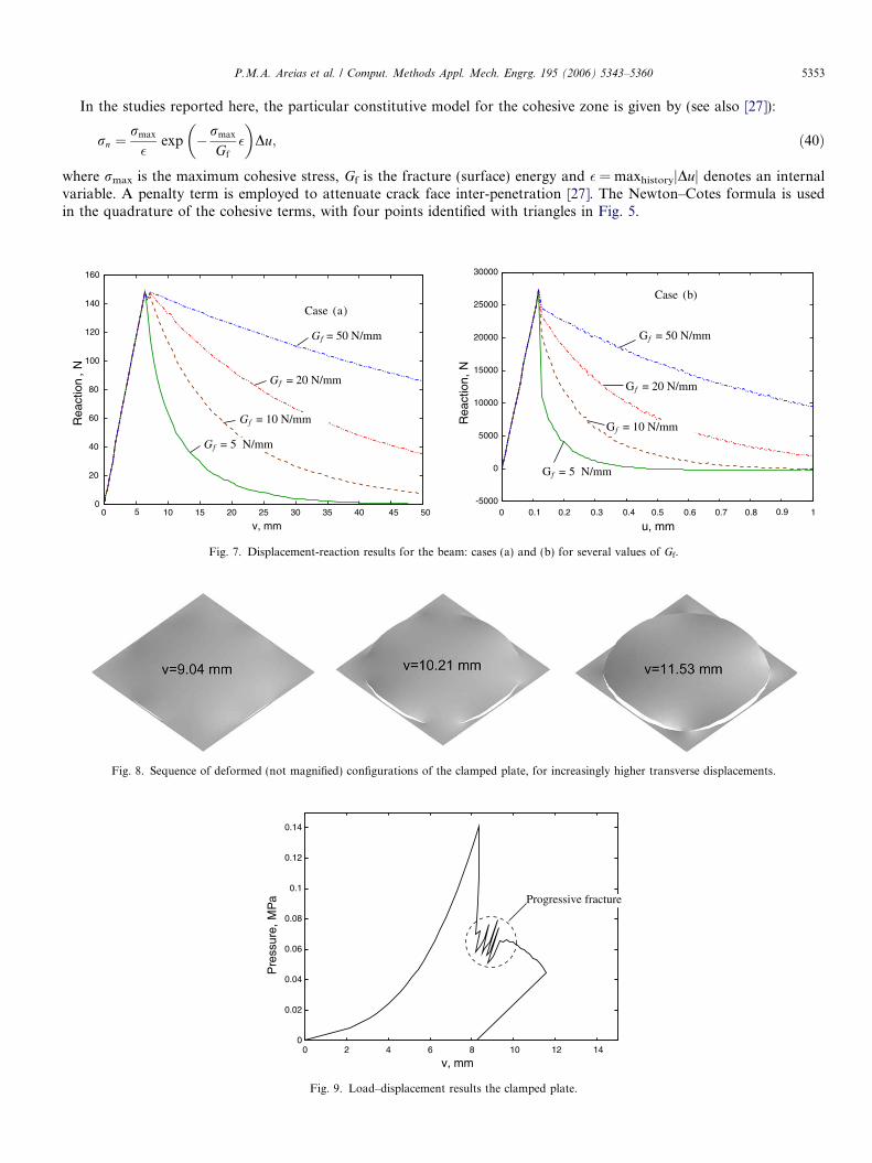
where rmax is the maximum cohesive stress, Gf is the fracture (surface) energy and � = maxhistoryjDuj denotes an internalvariable. A penalty term is employed to attenuate crack face inter-penetration [27]. The Newton–Cotes formula is usedin the quadrature of the cohesive terms, with four points identified with triangles in Fig. 5.

0 45 50

v, mm

Case (a)

160

140

120

100

80

60

40

20

0 10 15 20 25 30 35 40

Gf = 5 N/mm

Gf = 50 N/mm

Gf = 20 N/mm

Gf = 10 N/mmRea

ctio

n,

N

0.40 0.1 0.2 0.3 0.5 0.6 0.80.7 1-5000

0

5000

10000

15000

20000

25000

30000

Gf = 50 N/mm

Gf = 20 N/mm

Gf = 10 N/mm

Gf = 5 N/mm

Case (b)

u, mm

Rea

ctio

n,N

0.95

Fig. 7. Displacement-reaction results for the beam: cases (a) and (b) for several values of Gf.

Fig. 8. Sequence of deformed (not magnified) configurations of the clamped plate, for increasingly higher transverse displacements.

0

0.02

0.04

0.06

0.08

0.1

0.12

0.14

0 2 4 6 8 10 12 14

v, mm

Pre

ssur

e,M

Pa Progressive fracture

Fig. 9. Load–displacement results the clamped plate.


5. Numerical examples

The following numerical examples were run in the software SIMPLAS, created by the first author of this paper. A Post-script 3D post-processing software was also created by the same author. It was tested recently [7] using a non-linear EAS/XFEM variant of the Irons-Ahmad [28] shell element. The solution method is the residual-based damped Newton method(see also [29]) with arc-length continuation method.

5.1. Beam and plate brittle fracture

These two tests allow a simple assessment of the formulation and implementation, and in particular the inspection oflocking between the crack faces, as it occurs in the context of certain embedded crack techniques, see [30]. They also pro-vide an opportunity to test the cohesive law implementation. A noteworthy aspect of our implementation is that we candeactivate certain displacement components at the crack reference line (Dri = 0 for a given i = 1, . . . , 3), and thereforereproduce plastic hinges and other types of post-failure behavior. The beam and plate geometry and relevant propertiesare given in Fig. 6. The beam bending problem (corresponding to the case (a) in Fig. 6) is solved by constraining the relativedisplacement at the crack location in the lower cohesive line and allowing rotation using this line as axis.

For the beam problem, the reaction results are shown in Fig. 7. It can be seen that no spurious locking occurs, and thiscontrasts with un-modified versions of the embedded discontinuity method applied to plates [31].

For the plate, a regular mesh containing 80 · 80 elements is employed. The purpose is to verify what occurs in theabsence of cohesive forces and plasticity. In that case, oscillations occur after each subset of elements crack. A sequenceof deformed meshes is shown in Fig. 8. The corresponding central point displacement is also shown. The pressure versusdisplacement results are shown in Fig. 9. The effect of the discretization is apparent in this figure, with the oscillations in thepressure being induced by the sequential propagation through the elements.

5.2. Fracture of a hexcan

This problem was studied in Ref. [32] both experimentally and numerically. A hexagonal-base can, made of stainlesssteel type 316 is subjected to internal pressure up to fracture. From the test set of Ref. [32], we employ the specimenST103I. The fracture stress is 1 GPa. The relevant data for this test is briefly described in Fig. 10.

As can be seen, the crack propagates along the corners of the Hexcan, a fact that was observed experimentally (Fig. 11).

Fig. 10. Hexcan geometry and relevant properties.

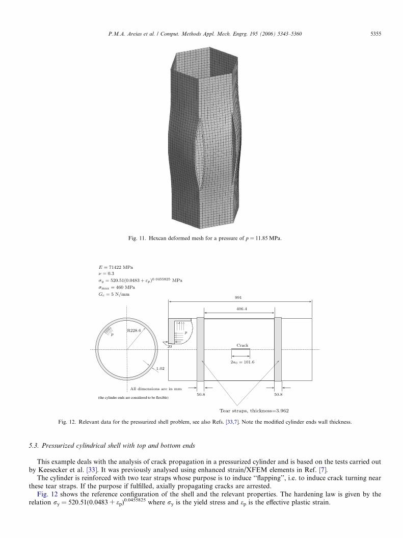
Fig. 11. Hexcan deformed mesh for a pressure of p = 11.85 MPa.

Fig. 12. Relevant data for the pressurized shell problem, see also Refs. [33,7]. Note the modified cylinder ends wall thickness.


5.3. Pressurized cylindrical shell with top and bottom ends

This example deals with the analysis of crack propagation in a pressurized cylinder and is based on the tests carried outby Keesecker et al. [33]. It was previously analysed using enhanced strain/XFEM elements in Ref. [7].

The cylinder is reinforced with two tear straps whose purpose is to induce ‘‘flapping’’, i.e. to induce crack turning nearthese tear straps. If the purpose if fulfilled, axially propagating cracks are arrested.

Fig. 12 shows the reference configuration of the shell and the relevant properties. The hardening law is given by therelation ry = 520.51(0.0483 + ep)0.0455825 where ry is the yield stress and ep is the effective plastic strain.

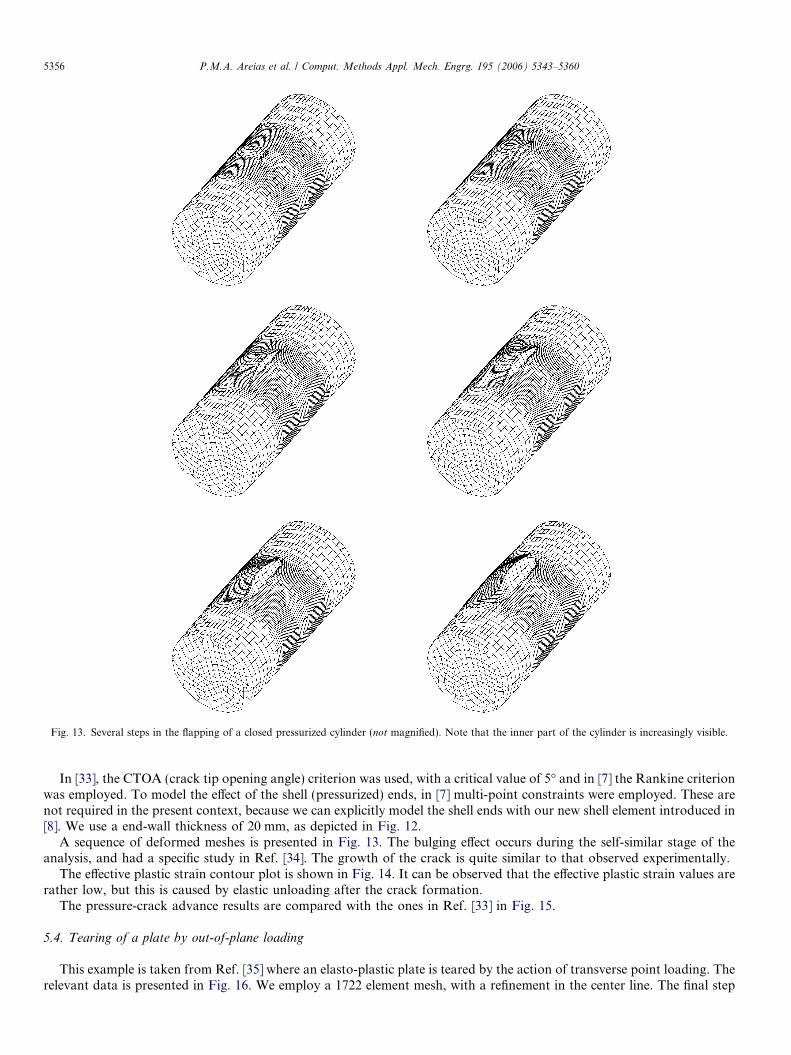
Fig. 13. Several steps in the flapping of a closed pressurized cylinder (not magnified). Note that the inner part of the cylinder is increasingly visible.


In [33], the CTOA (crack tip opening angle) criterion was used, with a critical value of 5� and in [7] the Rankine criterionwas employed. To model the effect of the shell (pressurized) ends, in [7] multi-point constraints were employed. These arenot required in the present context, because we can explicitly model the shell ends with our new shell element introduced in[8]. We use a end-wall thickness of 20 mm, as depicted in Fig. 12.

A sequence of deformed meshes is presented in Fig. 13. The bulging effect occurs during the self-similar stage of theanalysis, and had a specific study in Ref. [34]. The growth of the crack is quite similar to that observed experimentally.

The effective plastic strain contour plot is shown in Fig. 14. It can be observed that the effective plastic strain values arerather low, but this is caused by elastic unloading after the crack formation.

The pressure-crack advance results are compared with the ones in Ref. [33] in Fig. 15.

5.4. Tearing of a plate by out-of-plane loading

This example is taken from Ref. [35] where an elasto-plastic plate is teared by the action of transverse point loading. Therelevant data is presented in Fig. 16. We employ a 1722 element mesh, with a refinement in the center line. The final step

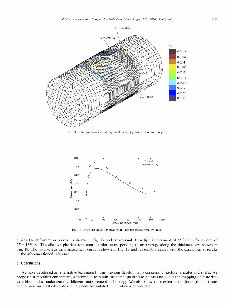
Fig. 14. Effective (averaged along the thickness) plastic strain contour plot.

0

0.05

0.1

0.15

0.2

0.25

0.3

0.35

40 60 80 100 120 140 160 180

Pre

ssur

e, M

Pa

Crack advance, mm

This work

Experimental

Fig. 15. Pressure-crack advance results for the pressurized cylinder.


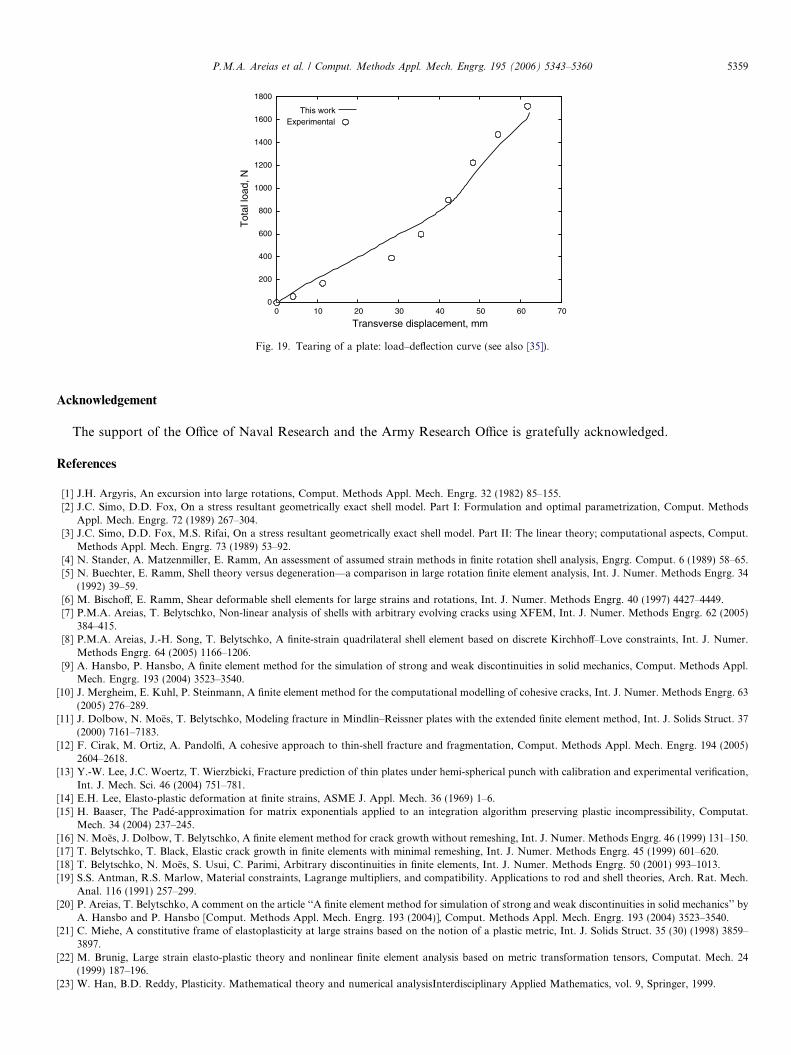
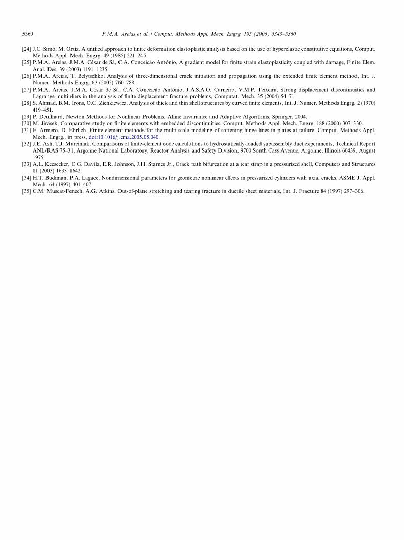
during the deformation process is shown in Fig. 17 and corresponds to a tip displacement of 65.87 mm for a load of2F = 1650 N. The effective plastic strain contour plot, corresponding to an average along the thickness, are shown inFig. 18. The load versus tip displacement curve is shown in Fig. 19 and reasonably agrees with the experimental resultsin the aforementioned reference.

6. Conclusions

We have developed an alternative technique to our previous developments concerning fracture in plates and shells. Weproposed a modified enrichment, a technique to retain the same quadrature points and avoid the mapping of historicalvariables, and a fundamentally different finite element technology. We also showed an extension to finite plastic strainsof the previous elasticity-only shell element formulated in curvilinear coordinates.

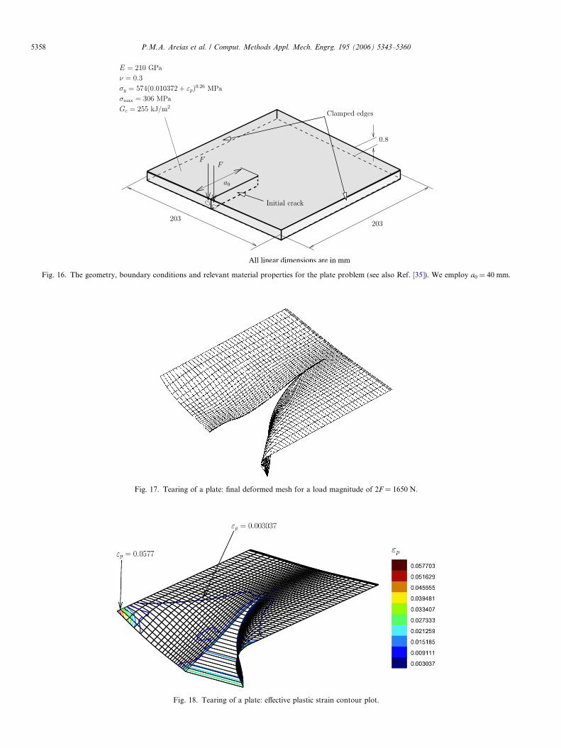
Fig. 16. The geometry, boundary conditions and relevant material properties for the plate problem (see also Ref. [35]). We employ a0 = 40 mm.

Fig. 17. Tearing of a plate: final deformed mesh for a load magnitude of 2F = 1650 N.

Fig. 18. Tearing of a plate: effective plastic strain contour plot.


0

200

400

600

800

1000

1200

1400

1600

1800

0 10 20 30 40 50 60 70

Tot

al lo

ad, N

Transverse displacement, mm

This workExperimental

Fig. 19. Tearing of a plate: load–deflection curve (see also [35]).


Acknowledgement

The support of the Office of Naval Research and the Army Research Office is gratefully acknowledged.

References

[1] J.H. Argyris, An excursion into large rotations, Comput. Methods Appl. Mech. Engrg. 32 (1982) 85–155.[2] J.C. Simo, D.D. Fox, On a stress resultant geometrically exact shell model. Part I: Formulation and optimal parametrization, Comput. Methods

Appl. Mech. Engrg. 72 (1989) 267–304.[3] J.C. Simo, D.D. Fox, M.S. Rifai, On a stress resultant geometrically exact shell model. Part II: The linear theory; computational aspects, Comput.

Methods Appl. Mech. Engrg. 73 (1989) 53–92.[4] N. Stander, A. Matzenmiller, E. Ramm, An assessment of assumed strain methods in finite rotation shell analysis, Engrg. Comput. 6 (1989) 58–65.[5] N. Buechter, E. Ramm, Shell theory versus degeneration—a comparison in large rotation finite element analysis, Int. J. Numer. Methods Engrg. 34

(1992) 39–59.[6] M. Bischoff, E. Ramm, Shear deformable shell elements for large strains and rotations, Int. J. Numer. Methods Engrg. 40 (1997) 4427–4449.[7] P.M.A. Areias, T. Belytschko, Non-linear analysis of shells with arbitrary evolving cracks using XFEM, Int. J. Numer. Methods Engrg. 62 (2005)

384–415.[8] P.M.A. Areias, J.-H. Song, T. Belytschko, A finite-strain quadrilateral shell element based on discrete Kirchhoff–Love constraints, Int. J. Numer.

Methods Engrg. 64 (2005) 1166–1206.[9] A. Hansbo, P. Hansbo, A finite element method for the simulation of strong and weak discontinuities in solid mechanics, Comput. Methods Appl.

Mech. Engrg. 193 (2004) 3523–3540.[10] J. Mergheim, E. Kuhl, P. Steinmann, A finite element method for the computational modelling of cohesive cracks, Int. J. Numer. Methods Engrg. 63

(2005) 276–289.[11] J. Dolbow, N. Moes, T. Belytschko, Modeling fracture in Mindlin–Reissner plates with the extended finite element method, Int. J. Solids Struct. 37

(2000) 7161–7183.[12] F. Cirak, M. Ortiz, A. Pandolfi, A cohesive approach to thin-shell fracture and fragmentation, Comput. Methods Appl. Mech. Engrg. 194 (2005)

2604–2618.[13] Y.-W. Lee, J.C. Woertz, T. Wierzbicki, Fracture prediction of thin plates under hemi-spherical punch with calibration and experimental verification,

Int. J. Mech. Sci. 46 (2004) 751–781.[14] E.H. Lee, Elasto-plastic deformation at finite strains, ASME J. Appl. Mech. 36 (1969) 1–6.[15] H. Baaser, The Pade-approximation for matrix exponentials applied to an integration algorithm preserving plastic incompressibility, Computat.

Mech. 34 (2004) 237–245.[16] N. Moes, J. Dolbow, T. Belytschko, A finite element method for crack growth without remeshing, Int. J. Numer. Methods Engrg. 46 (1999) 131–150.[17] T. Belytschko, T. Black, Elastic crack growth in finite elements with minimal remeshing, Int. J. Numer. Methods Engrg. 45 (1999) 601–620.[18] T. Belytschko, N. Moes, S. Usui, C. Parimi, Arbitrary discontinuities in finite elements, Int. J. Numer. Methods Engrg. 50 (2001) 993–1013.[19] S.S. Antman, R.S. Marlow, Material constraints, Lagrange multipliers, and compatibility. Applications to rod and shell theories, Arch. Rat. Mech.

Anal. 116 (1991) 257–299.[20] P. Areias, T. Belytschko, A comment on the article ‘‘A finite element method for simulation of strong and weak discontinuities in solid mechanics’’ by

A. Hansbo and P. Hansbo [Comput. Methods Appl. Mech. Engrg. 193 (2004)], Comput. Methods Appl. Mech. Engrg. 193 (2004) 3523–3540.[21] C. Miehe, A constitutive frame of elastoplasticity at large strains based on the notion of a plastic metric, Int. J. Solids Struct. 35 (30) (1998) 3859–

3897.[22] M. Brunig, Large strain elasto-plastic theory and nonlinear finite element analysis based on metric transformation tensors, Computat. Mech. 24

(1999) 187–196.[23] W. Han, B.D. Reddy, Plasticity. Mathematical theory and numerical analysisInterdisciplinary Applied Mathematics, vol. 9, Springer, 1999.


[24] J.C. Simo, M. Ortiz, A unified approach to finite deformation elastoplastic analysis based on the use of hyperelastic constitutive equations, Comput.Methods Appl. Mech. Engrg. 49 (1985) 221–245.

[25] P.M.A. Areias, J.M.A. Cesar de Sa, C.A. Conceicao Antonio, A gradient model for finite strain elastoplasticity coupled with damage, Finite Elem.Anal. Des. 39 (2003) 1191–1235.

[26] P.M.A. Areias, T. Belytschko, Analysis of three-dimensional crack initiation and propagation using the extended finite element method, Int. J.Numer. Methods Engrg. 63 (2005) 760–788.

[27] P.M.A. Areias, J.M.A. Cesar de Sa, C.A. Conceicao Antonio, J.A.S.A.O. Carneiro, V.M.P. Teixeira, Strong displacement discontinuities andLagrange multipliers in the analysis of finite displacement fracture problems, Computat. Mech. 35 (2004) 54–71.

[28] S. Ahmad, B.M. Irons, O.C. Zienkiewicz, Analysis of thick and thin shell structures by curved finite elements, Int. J. Numer. Methods Engrg. 2 (1970)419–451.

[29] P. Deuflhard, Newton Methods for Nonlinear Problems, Affine Invariance and Adaptive Algorithms, Springer, 2004.[30] M. Jirasek, Comparative study on finite elements with embedded discontinuities, Comput. Methods Appl. Mech. Engrg. 188 (2000) 307–330.[31] F. Armero, D. Ehrlich, Finite element methods for the multi-scale modeling of softening hinge lines in plates at failure, Comput. Methods Appl.

Mech. Engrg., in press, doi:10.1016/j.cma.2005.05.040.[32] J.E. Ash, T.J. Marciniak, Comparisons of finite-element code calculations to hydrostatically-loaded subassembly duct experiments, Technical Report

ANL/RAS 75–31, Argonne National Laboratory, Reactor Analysis and Safety Division, 9700 South Cass Avenue, Argonne, Illinois 60439, August1975.

[33] A.L. Keesecker, C.G. Davila, E.R. Johnson, J.H. Starnes Jr., Crack path bifurcation at a tear strap in a pressurized shell, Computers and Structures81 (2003) 1633–1642.

[34] H.T. Budiman, P.A. Lagace, Nondimensional parameters for geometric nonlinear effects in pressurized cylinders with axial cracks, ASME J. Appl.Mech. 64 (1997) 401–407.

[35] C.M. Muscat-Fenech, A.G. Atkins, Out-of-plane stretching and tearing fracture in ductile sheet materials, Int. J. Fracture 84 (1997) 297–306.

http://dx.doi.org/10.1016/j.cma.2005.05.040

Documents

Analysis of fracture in thin shells by overlapping paired ... · Analysis of fracture in thin shells by overlapping paired elements Pedro M.A. Areias, J.H. Song, Ted Belytschko *