1

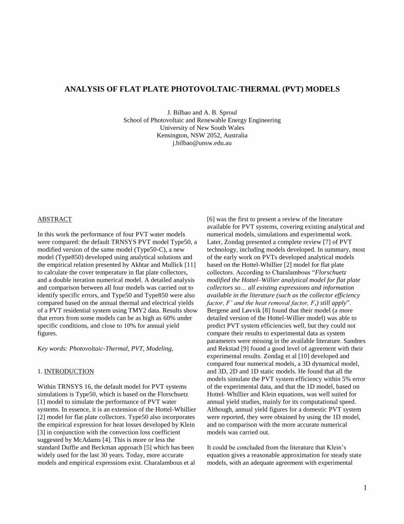
ANALYSIS OF FLAT PLATE PHOTOVOLTAIC-THERMAL (PVT) MODELS

J. Bilbao and A. B. Sproul

School of Photovoltaic and Renewable Energy Engineering

University of New South Wales

Kensington, NSW 2052, Australia

j.bilbao@unsw.edu.au

ABSTRACT

In this work the performance of four PVT water models

were compared: the default TRNSYS PVT model Type50, a

modified version of the same model (Type50-C), a new

model (Type850) developed using analytical solutions and

the empirical relation presented by Akhtar and Mullick [11]

to calculate the cover temperature in flat plate collectors,

and a double iteration numerical model. A detailed analysis

and comparison between all four models was carried out to

identify specific errors, and Type50 and Type850 were also

compared based on the annual thermal and electrical yields

of a PVT residential system using TMY2 data. Results show

that errors from some models can be as high as 60% under

specific conditions, and close to 10% for annual yield

figures.

Key words: Photovoltaic-Thermal, PVT, Modeling,

1. INTRODUCTION

Within TRNSYS 16, the default model for PVT systems

simulations is Type50, which is based on the Florschuetz

[1] model to simulate the performance of PVT water

systems. In essence, it is an extension of the Hottel-Whillier

[2] model for flat plate collectors. Type50 also incorporates

the empirical expression for heat losses developed by Klein

[3] in conjunction with the convection loss coefficient

suggested by McAdams [4]. This is more or less the

standard Duffie and Beckman approach [5] which has been

widely used for the last 30 years. Today, more accurate

models and empirical expressions exist. Charalambous et al

[6] was the first to present a review of the literature

available for PVT systems, covering existing analytical and

numerical models, simulations and experimental work.

Later, Zondag presented a complete review [7] of PVT

technology, including models developed. In summary, most

of the early work on PVTs developed analytical models

based on the Hottel-Whillier [2] model for flat plate

collectors. According to Charalambous “Florschuetz

modified the Hottel–Willier analytical model for flat plate

collectors so… all existing expressions and information

available in the literature (such as the collector efficiency

factor, F’ and the heat removal factor, Fr) still apply”.

Bergene and Løvvik [8] found that their model (a more

detailed version of the Hottel-Willier model) was able to

predict PVT system efficiencies well, but they could not

compare their results to experimental data as system

parameters were missing in the available literature. Sandnes

and Rekstad [9] found a good level of agreement with their

experimental results. Zondag et al [10] developed and

compared four numerical models, a 3D dynamical model,

and 3D, 2D and 1D static models. He found that all the

models simulate the PVT system efficiency within 5% error

of the experimental data, and that the 1D model, based on

Hottel–Whillier and Klein equations, was well suited for

annual yield studies, mainly for its computational speed.

Although, annual yield figures for a domestic PVT system

were reported, they were obtained by using the 1D model,

and no comparison with the more accurate numerical

models was carried out.

It could be concluded from the literature that Klein’s

equation gives a reasonable approximation for steady state

models, with an adequate agreement with experimental

2

data. However, Klein’s equation has not been tested against

annual yield results using experimental data or other

models. Moreover, according to Akhtar and Mullick [11],

Klein’s equation can produce errors of up to 10% in the

estimation of the top losses of a flat plate collector for high

plate temperatures, and around 5% for low plate

temperatures. In the same publication, Akhtar and Mullick

propose a new experimental relation to estimate the cover

temperature of a flat plate hot water system, in replacement

of Klein’s equation.

The objective of this work was to check the results of

different PVT models for collectors with and without a

cover. The analysis is focused on heat transfer from the top

surfaces of the collector, and therefore is relevant not just

for PVT water models but also PVT air. Particular attention

was paid to the performance of the standard model included

in TRNSYS, Type50 (and therefore Florschuetz and Klein

approach), against more accurate models, like the developed

Type850. Section two of this paper will describe in detail all

the models used in the work. In section three, the results of

several simulations between the models are presented,

including in-depth comparisons. Finally, in section four,

several conclusions and recommendations are provided. The

nomenclature is presented in section five.

2. DESCRIPTION OF PVT MODELS USED

A total of four PVT models were used in this work:

1) a numerical model using a double iteration solving

method of the heat transfer equations;

2) a numerical model, with a single iteration process,

where the cover temperature is calculated using the

relations developed by Akhtar and Mullick (Type850);

3) Type50 model (part of the standard TRNSYS software

package);

4) a modified version of Type50, in which F’ is calculated

for each simulation (called Type50-C).

All of the above models were implemented in Excel. These

models can generate quick steady state results under

particular conditions, and are used for detailed comparison

between the models, but are not suited for year long

simulations.

In order to study the effects of the approximations made in

Type50 on an annual yield basis, model number 2, called

Type850 from now onwards (work of the authors), was also

implemented in TRNSYS, due to its simplicity and good

accuracy when compared to the double iteration numerical

model (model number 1).

In the following sections all the models will be described in

more detail.

2.1 Double iteration numerical model (implemented in

Excel)

As its name implies, in this numerical model a double

iteration is required to calculate all the heat transfer

equations for the case of the PVT collector with cover. First,

the initial cover and absorber plate temperatures are set: for

the cover temperature the ambient temperature plus one

degree is used, and 100°C is used for the plate temperature,

which is close to the stagnation temperature.

With Tp and Tc, the Nusselt number of the air in the cavity is

estimated using Buchberg [12] relation, in order to calculate

the convection losses between both surfaces. Also, from

Cooper [13] the relations from the Tables of Thermal

Properties of Gases, U.S. Department of Commerce, were

used to model the property of the air in the cavity between

the plate and cover, according to the average temperature of

both surfaces. Then all the convective and radiative losses

are calculated and combined as per equation 1, in order to

estimate the total losses of the PVT module.

(1) [( )

( ) ]

where Urpc and Ucpc are the radiative and convective losses

between the plate and the cover, Urcs and Uw are the

radiative and convection losses of the top cover, and UBE is

the back and edge losses, constant during the simulation.

Then, the thermal efficiency factors are calculated, starting

by F’, using the equation for collectors with square

channels:

(2)

⁄

where hf is the total thermal conductance between the plate

and the fluid. Fr is calculated using the standard equation in

[5]. Then the electrical and thermal useful energy rates per

unit of area are calculated using:

(3) [ ( )]

(4) ( ( ))

Notice that for the thermal energy output, the absorbed solar

energy is corrected using the electrical energy produced by

the PV cells. The mean plate temperature and the cover

temperature are calculated using an energy balance

approach:

(5)

(6) ( ) ( )

( )

3

From this point onwards, the new values of Tp or Tc can be

used to recalculate all the equations until the chosen

variables converge. Then the same process can be used with

the other variable until it converges. This double iteration

process will have to be repeated until the error in both

variables is small. If done manually it can be a lengthy

process, but in excel the solver routine can be used, and

solutions are found automatically.

For the case of the PVT collector without a cover, there is

no need to estimate the cover temperature and a single

iteration approach is enough to accurately calculate all the

heat losses. The simulation starts with an initial estimation

of the plate temperature. Then, the total losses (UL) are

calculated by adding the radiation (Urcs) and convection

(Uw) losses from the top of the panel, plus the back and

edge losses (UBE).

Once the losses are calculated, the same equations used for

the collector with a cover (Eqs. 2, 3, 4, and 5) are used to

calculate F’, Fr, Qe, Qu, and Tp, but the cover temperature is

replaced by the plate temperature when required.

2.2 Single iteration model, TYPE850 (implemented in

Excel and TRNSYS)

In this model, the empirical relations developed by Akhtar

and Mullick [11] to estimate the cover temperature of Flat

Plate Solar Collectors were used. One of the strengths of

these empirical relations is that they allow for the use of the

Sky Temperature, and therefore, the correct calculation of

the radiation losses.

The algorithm and equations used in this model are exactly

the same as in the double iteration model, except for the use

of the cover temperature equations. This allows having one

less unknown variable and therefore, only a single iteration

process can be used. This iteration allows for the self-

correction of the thermal energy output (eq. 4) and UL, so

there is no need to use Florschuetz’s proposed adjustment

for PVT panels. This also allows the use of Akhtar and

Mullick equations without the need of any modifications.

For the case of the PVT collector without a cover, the

algorithm and equations are the same as for the first model.

2.3 Standard PVT model, Type50 (implemented in Excel,

existing in TRNSYS)

As explained above, Type50 is a very close implementation

of Florschuetz [1] work. Type50 has four modes of

operation for flat plate collectors, and other modes for

concentrating collectors not reviewed in this paper. In this

work, MODE 2 will be used because it proved to be more

stable than the others. However, in MODE 2 the angular

dependence of the cover transmisivity is considered

constant (unlike MODE4 which includes the incident angle

modifiers, but was unable to converge), so adjustments were

introduced to the solar irradiance data to take into account

the angle of incidence to make a fair comparison with the

rest of the models.

Type 50 also uses a single iteration approach to solve the

heat transfer equations, thanks to the use of Klein’s equation

to estimate the top cover losses.

Some key Type50 model details and differences with the

original Florschuetz work are:

- The algorithm runs for three iterations (controlled by an

internal counter) for each time step, after which the

program exits the simulation with whatever values are

achieved.

- Equations for the calculation of F’ were not implemented

in Type50, as F’ is a given parameter to the model and

remains constant through the whole simulation.

- The mean fluid temperature is approximated as the

average of the inlet and outlet temperature, which is

different to the true analytical value.

- The cell temperature is calculated at the end of each time

step and is used only for output purposes and not as part

of the internal calculations.

- The thermal losses are calculated using the empirical

equation developed by Klein [3], which does not take into

account the sky temperature

- In the implementation of Klein’s equation in Type50, the

mean water temperature is used instead of the mean plate

temperature.

In the Excel implementation of this model, the three

iterations limit was not used, and the algorithm runs until

the values converge.

2.4 Modified Standard PVT model, Type50-C

(implemented in Excel)

This type uses the same equations as Type50, but F’ is

calculated using equation 2 for each simulation. This allows

an accurate value of the efficiency factor to be calculated

depending on the calculated heat losses. Although this is

certainly an improvement over Type50, it also makes the

model more susceptive to the possible errors introduced in

the calculation of the top losses by Klein’s equation.

3. RESULTS

In the first three parts of this section, all the models using

empirical equations (models 2 to 4) are compared in detail

against the double iteration numerical model (model 1),

studying for example the impact of the simplifications made

4

in Type50, particularly, the use of the constant F’

coefficient. For the purpose of these comparisons, the Excel

implementations of the models were used, with the

parameters at design conditions, shown in Table 1.

TABLE 1: PARAMETERS AT DESIGN CONDITIONS

FOR THE CALCULATION OF F’

Parameter Value

No Cover

Value

Cover Description

H 800 800 Solar Radiation (W/m2)

Vw 2 2 Wind velocity (m/s)

Tin 20 20 Inlet Temperature (°C)

Tamb 20 20 Amb. Temperature (°C)

B 30 30 Panel Tilt (degrees)

εp 0.850 0.850 Collector Plate Emissivity

εg - 0.850 Glass cover Emissivity

α 0.900 0.900 Effective Absorptance

τ 0.920 0.846 Total Transmittance

ηr 0.144 0.144 Cell Eff. at Ref. Temp.

βr 0.0048 0.0048 Cell Temp. Coef. (1/K)

ů 0.020 0.011 Mass Flowrate (Kg/s.m2)

hf 56.923 43.258 Plate to Fluid (W/m2.C)

UL 18.596 4.622 Total Losses (W/m2.C)

F’ 0.754 0.903 Collector Eff. Factor

In part 3.4 of this section, Type50 and Type850 are

compared on an annual basis, using a simulation of a

residential hot water system in TRNSYS.

3.1 Effects of F’ simplification

F’ was calculated at the design conditions (see Table 1) and

kept constant in Type50, but it was calculated for each

simulation in Type50-C. The value of Fr was compared for

both models to quantify the errors of the simplification,

because is directly proportional to the useful thermal energy

Qu. Results for different combinations of ambient

temperature, inlet temperature and wind velocity are shown

in Figure 1 and Figure 2 respectively, for both type of

collectors (with and without a cover).

For the panel without a cover, changes in the wind speed

have an important impact in the calculation of Fr, so the

changes in the inlet and ambient temperatures are dwarfed

in comparison. This is a logical result, because convection

losses are dominant in a coverless panel. When the panel

operates close to the “design conditions”, the errors are

small and less than 5%, but at high wind speeds errors can

escalate up to 30%. The problem of Klein’s equation for

coverless panels as implemented in Type50, is the use of the

mean fluid temperature instead of the correct mean plate

temperature. The effects of a constant F’ are less

pronounced in PVT modules with a cover, as the maximum

Fig. 1: Fr percentage error for fixed ambient temperature

Fig. 2: Fr percentage error for fixed inlet temperature.

14

16

18

20

22

24

26

28

30

0 1 2 3 4 5 6 7 8 9 10

Tin

( C

)

Wind Velocity (m/s)

a) Fr percentage error (Tamb = Tsky = 20 C, N = 0)

5%-10%

0%-5%

-5%-0%

-10%--5%

-15%--10%

-20%--15%

-25%--20%

-30%--25%

-35%--30%

15

20

25

30

35

40

45

50

55

0 2 4 6 8 10

Tin

( C

)

Wind Velocity (m/s)

b) Fr percentage error (Tamb = Tsky = 20 C, N = 1)

2%-3%

1%-2%

0%-1%

-1%-0%

-2%--1%

-3%--2%

-4%--3%

-5%--4%

-6%--5%

14

16

18

20

22

24

26

28

30

0 1 2 3 4 5 6 7 8 9 10

Ta

mb

( C

)

Wind Velocity (m/s)

a) Fr percentage error (Tin = 20 C, N = 0)

5%-10%

0%-5%

-5%-0%

-10%--5%

-15%--10%

-20%--15%

-25%--20%

-30%--25%

-35%--30%

14

16

18

20

22

24

0 2 4 6 8 10

Ta

mb

( C

)

Wind Velocity (m/s)

b) Fr percentage error (Tin = 20 C, N = 1)

1.5%-2.0%

1.0%-1.5%

0.5%-1.0%

0.0%-0.5%

-0.5%-0.0%

-1.0%--0.5%

-1.5%--1.0%

-2.0%--1.5%

-2.5%--2.0%

-3.0%--2.5%

5

error is kept below 6%. In this case, the inlet temperature is

shown to have an equally important effect to the wind

velocity. The results suggest that the effects of using a fixed

F’ are reasonable for a PVT system with a cover.

3.2 Comparison of Type50, 50-C, and 850 against Model 1

Klein’s equation is close to the correct calculation of top

losses when ambient temperature is similar to sky

temperature (cloudy sky), so Type50 should perform well

under these conditions. However, PVT panels have high

emissivity –unlike solar hot water collectors that usually

have selective surfaces– so it’s expected that changes in the

sky temperature will produce noticeable effects in the

performance of the models even for panels with covers. The

model using Akhtar and Mullick equations was also

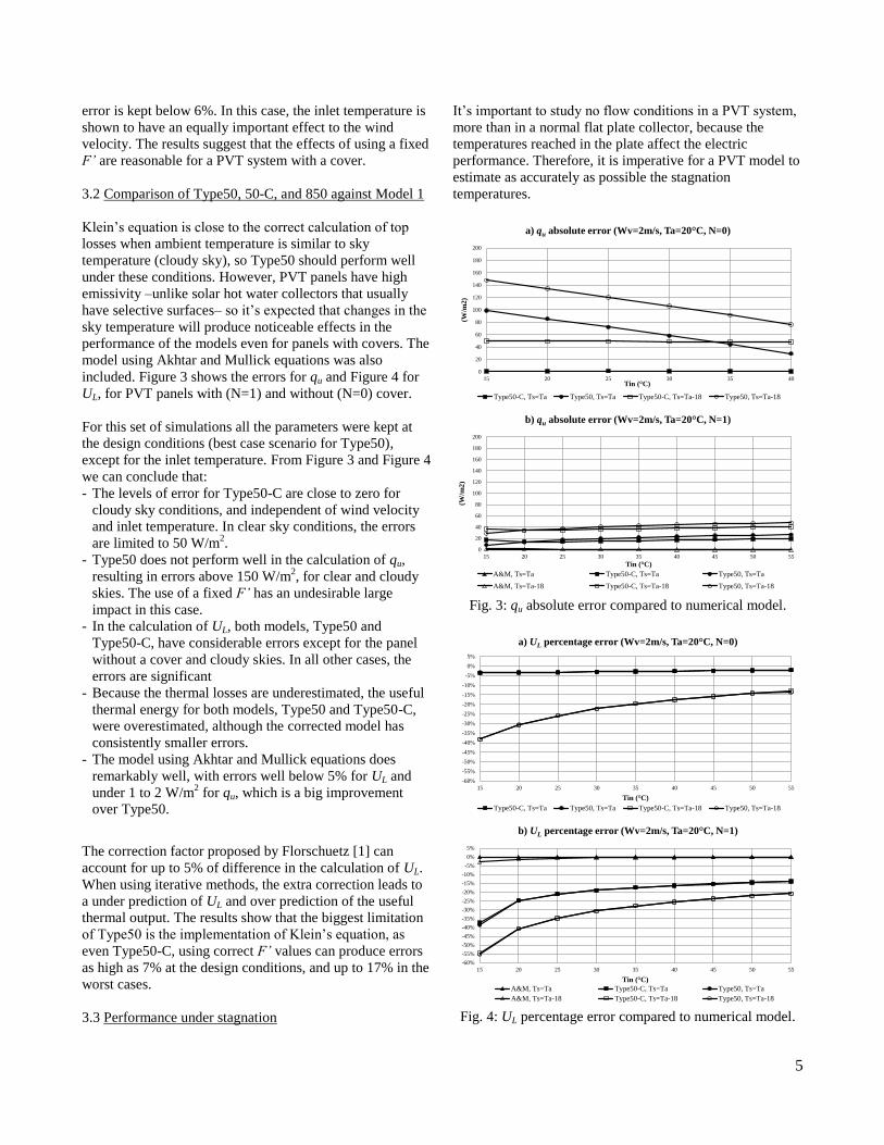
included. Figure 3 shows the errors for qu and Figure 4 for

UL, for PVT panels with (N=1) and without (N=0) cover.

For this set of simulations all the parameters were kept at

the design conditions (best case scenario for Type50),

except for the inlet temperature. From Figure 3 and Figure 4

we can conclude that:

- The levels of error for Type50-C are close to zero for

cloudy sky conditions, and independent of wind velocity

and inlet temperature. In clear sky conditions, the errors

are limited to 50 W/m2.

- Type50 does not perform well in the calculation of qu,

resulting in errors above 150 W/m2, for clear and cloudy

skies. The use of a fixed F’ has an undesirable large

impact in this case.

- In the calculation of UL, both models, Type50 and

Type50-C, have considerable errors except for the panel

without a cover and cloudy skies. In all other cases, the

errors are significant

- Because the thermal losses are underestimated, the useful

thermal energy for both models, Type50 and Type50-C,

were overestimated, although the corrected model has

consistently smaller errors.

- The model using Akhtar and Mullick equations does

remarkably well, with errors well below 5% for UL and

under 1 to 2 W/m2 for qu, which is a big improvement

over Type50.

The correction factor proposed by Florschuetz [1] can

account for up to 5% of difference in the calculation of UL.

When using iterative methods, the extra correction leads to

a under prediction of UL and over prediction of the useful

thermal output. The results show that the biggest limitation

of Type50 is the implementation of Klein’s equation, as

even Type50-C, using correct F’ values can produce errors

as high as 7% at the design conditions, and up to 17% in the

worst cases.

3.3 Performance under stagnation

It’s important to study no flow conditions in a PVT system,

more than in a normal flat plate collector, because the

temperatures reached in the plate affect the electric

performance. Therefore, it is imperative for a PVT model to

estimate as accurately as possible the stagnation

temperatures.

Fig. 3: qu absolute error compared to numerical model.

Fig. 4: UL percentage error compared to numerical model.

0

20

40

60

80

100

120

140

160

180

200

15 20 25 30 35 40

(W/m

2)

Tin ( C)

a) qu absolute error (Wv=2m/s, Ta=20 C, N=0)

Type50-C, Ts=Ta Type50, Ts=Ta Type50-C, Ts=Ta-18 Type50, Ts=Ta-18

0

20

40

60

80

100

120

140

160

180

200

15 20 25 30 35 40 45 50 55

(W/m

2)

Tin ( C)

b) qu absolute error (Wv=2m/s, Ta=20 C, N=1)

A&M, Ts=Ta Type50-C, Ts=Ta Type50, Ts=Ta

A&M, Ts=Ta-18 Type50-C, Ts=Ta-18 Type50, Ts=Ta-18

-60%

-55%

-50%

-45%

-40%

-35%

-30%

-25%

-20%

-15%

-10%

-5%

0%

5%

15 20 25 30 35 40 45 50 55

Tin ( C)

a) UL percentage error (Wv=2m/s, Ta=20 C, N=0)

Type50-C, Ts=Ta Type50, Ts=Ta Type50-C, Ts=Ta-18 Type50, Ts=Ta-18

-60%

-55%

-50%

-45%

-40%

-35%

-30%

-25%

-20%

-15%

-10%

-5%

0%

5%

15 20 25 30 35 40 45 50 55

Tin ( C)

b) UL percentage error (Wv=2m/s, Ta=20 C, N=1)

A&M, Ts=Ta Type50-C, Ts=Ta Type50, Ts=Ta

A&M, Ts=Ta-18 Type50-C, Ts=Ta-18 Type50, Ts=Ta-18

6

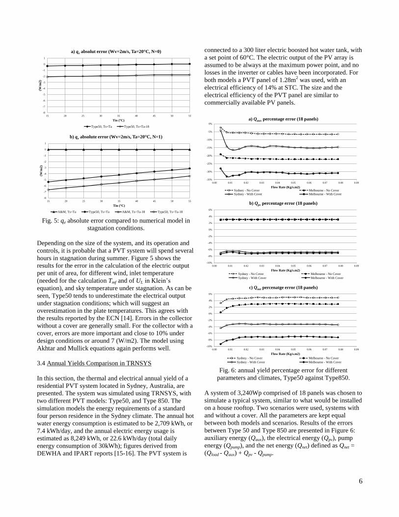
Fig. 5: qe absolute error compared to numerical model in

stagnation conditions.

Depending on the size of the system, and its operation and

controls, it is probable that a PVT system will spend several

hours in stagnation during summer. Figure 5 shows the

results for the error in the calculation of the electric output

per unit of area, for different wind, inlet temperature

(needed for the calculation Tmf and of UL in Klein’s

equation), and sky temperature under stagnation. As can be

seen, Type50 tends to underestimate the electrical output

under stagnation conditions; which will suggest an

overestimation in the plate temperatures. This agrees with

the results reported by the ECN [14]. Errors in the collector

without a cover are generally small. For the collector with a

cover, errors are more important and close to 10% under

design conditions or around 7 (W/m2). The model using

Akhtar and Mullick equations again performs well.

3.4 Annual Yields Comparison in TRNSYS

In this section, the thermal and electrical annual yield of a

residential PVT system located in Sydney, Australia, are

presented. The system was simulated using TRNSYS, with

two different PVT models: Type50, and Type 850. The

simulation models the energy requirements of a standard

four person residence in the Sydney climate. The annual hot

water energy consumption is estimated to be 2,709 kWh, or

7.4 kWh/day, and the annual electric energy usage is

estimated as 8,249 kWh, or 22.6 kWh/day (total daily

energy consumption of 30kWh); figures derived from

DEWHA and IPART reports [15-16]. The PVT system is

connected to a 300 liter electric boosted hot water tank, with

a set point of 60°C. The electric output of the PV array is

assumed to be always at the maximum power point, and no

losses in the inverter or cables have been incorporated. For

both models a PVT panel of 1.28m2 was used, with an

electrical efficiency of 14% at STC. The size and the

electrical efficiency of the PVT panel are similar to

commercially available PV panels.

Fig. 6: annual yield percentage error for different

parameters and climates, Type50 against Type850.

A system of 3,240Wp comprised of 18 panels was chosen to

simulate a typical system, similar to what would be installed

on a house rooftop. Two scenarios were used, systems with

and without a cover. All the parameters are kept equal

between both models and scenarios. Results of the errors

between Type 50 and Type 850 are presented in Figure 6:

auxiliary energy (Qaux), the electrical energy (Qpv), pump

energy (Qpump), and the net energy (Qnet) defined as Qnet =

(Qload - Qaux) + Qpv - Qpump.

-8

-7

-6

-5

-4

-3

-2

-1

0

1

15 20 25 30 35 40 45 50 55

(W/m

2)

Tin ( C)

a) qe absolut error (Wv=2m/s, Ta=20 C, N=0)

Type50, Ts=Ta Type50, Ts=Ta-18

-8

-7

-6

-5

-4

-3

-2

-1

0

1

15 20 25 30 35 40 45 50 55

(W/m

2)

Tin ( C)

b) qe absolute error (Wv=2m/s, Ta=20 C, N=1)

A&M, Ts=Ta Type50, Ts=Ta A&M, Ts=Ta-18 Type50, Ts=Ta-18

-35%

-30%

-25%

-20%

-15%

-10%

-5%

0%

0.00 0.01 0.02 0.03 0.04 0.05 0.06 0.07 0.08 0.09

Flow Rate (Kg/s.m2)

a) Qaux percentage error (18 panels)

Sydney - No Cover Melbourne - No Cover

Sydney - With Cover Melbourne - With Cover

-10%

-8%

-6%

-4%

-2%

0%

2%

4%

6%

0.00 0.01 0.02 0.03 0.04 0.05 0.06 0.07 0.08 0.09

Flow Rate (Kg/s.m2)

b) Qpv percentage error (18 panels)

Sydney - No Cover Melbourne - No Cover

Sydney - With Cover Melbourne - With Cover

-10%

-8%

-6%

-4%

-2%

0%

2%

4%

6%

0.00 0.01 0.02 0.03 0.04 0.05 0.06 0.07 0.08 0.09

Flow Rate (Kg/s.m2)

c) Qnet percenatge error (18 panels)

Sydney - No Cover Melbourne - No Cover

Sydney - With Cover Melbourne - With Cover

7

The results show that Type50 is consistently over predicting

the thermal output, and therefore, the auxiliary energy

required is under predicted with respect to Type 850. Errors

for the annual amount of required auxiliary energy are

around 15% for panels with cover and 6% for panels

without a cover. On the electrical output, Type50 with a

cover under predicts the annual yield by 7% and over

predicts the panel without a cover by 3%, i.e., Type50 with

cover runs “hotter” than Type850, and Type50 without a

cover runs “cooler”. The energy required by the pump is in

direct relation of the amount of hours that the thermal

system was working. In this scenario, Type50 with and

without a cover runs the pump 7% and 20% longer time

frames, respectively. Some findings might seem

contradictory, but in reality, they reflect how a PVT system

performance changes depending on the size of the system,

its operation, and in particular, if it was carried out as an

individual unit or as part of a system. This reaffirms the

point that PVT systems performance and design should be

always analyzed in the context of an application.

4. CONCLUSIONS

From the specific analysis of Type50, we can summarize

the shortcomings of the model as:

- The value of F’ is assumed as a constant parameter,

independent of the changes in the total losses UL which

depends on ambient conditions (wind speed, ambient

temperature) and fluid temperature. Errors of up to 10%

are expected when maintaining F’ constant.

- Sky temperature is not used for the calculation of

radiation losses. This is particularly important in PVT

systems, compared to hot water collectors, because PV

panels have high emissivity.

- The model implements the original equation of Klein [3]

using Tmf instead of Tp. This leads to more errors and

instabilities when Tmf < Tamb. For PVT systems with small

areas, this is not an uncommon scenario (Akhtar and

Mullick equation has the same problem when Tp < Tamb,

less often).

- The model uses Florschuetz’s correction factor for UL to

account for the electrical output of the system. However,

it is considered that this correction factor should not be

used.

- As a result, Type50 calculation of UL can produce errors

of up to 60% in the worst cases.

- Although 3 iterations should be enough for the model to

converge most of the times, there is no guarantee that

moderate errors could not be happening in some time

steps.

From the annual yield analysis we can conclude that:

- Even though the errors are in general smaller than in the

specific analysis, some serious differences are still

present, specifically regarding the thermal output and its

effect in the auxiliary power, with maximum errors of

16% for Sydney climate and 32% for Melbourne climate.

- Type50 underestimates the thermal losses of the panel and

therefore the model overestimates the thermal output. This

results in the controller running the pump more hours

during the year, which leads to large errors in the

calculations of the annual energy required by the pump

system.

- PV electric energy output errors are of the order of ±5%,

which can be considered acceptable.

- As for any summary of data, the annual yield gives an

average of the errors, possibly masking large differences

in the operation of the system in a day to day basis.

In conclusion, it appears clear that Type50 offers several

limitations where high levels of accuracy are required.

Although the electrical output accuracy is worrying at a

model level, the errors in the annual yield case are

acceptable. The errors on the thermal output can be above

10%, which introduces a higher level of uncertainty in the

design of a system. On the other hand, the work proposed

by Akhtar and Mullick [7] proved to be exceptionally

accurate when compared to the complete numerical

solution. Finally, it is recommended that system analyses

with whole year simulations (using TMY2 data or similar)

should be used to study the performance of PVT systems

and to compare different models.

5. NOMENCLATURE

B tilt angle of panel

F’ collector efficiency factor

Fr collector heat removal factor

H total solar radiation incident on collector

N number of covers

qu useful thermal energy collection rate per unit area

qe useful electrical energy collection rate per unit area

S absorbed solar radiation per unit area

Ta ambient temperature

Tc cover temperature

Tin inlet temperature

Tp mean plate temperature

Tr PV reference temperature

Ts sky temperature

hf thermal conductance between absorber and fluid

UBE bottom and edges heat loss coefficient

UL overall heat loss coefficient

Ucpc convection heat loss coefficient among plate and cover

Urcs radiation heat loss coefficient between cover and sky

Urpc radiation heat loss coefficient between plate and cover

Uw convection heat loss coefficient due to wind speed

ů mass flow rate

Vw wind velocity

α effective absorptance of collector absorber

8

βr temperature coefficient of solar cell

σ Stefan–Boltzmann constant

εg glass emissivity

εp absorber plate emissivity

ηr cell efficiency at reference temperature

τ transmittance of collector glass cover

6. REFERENCES

(1) Florschuetz, L. W., Extension of the Hottel-Whillier

model to the analysis of combined photovoltaic/thermal flat

plate collectors, Solar Energy 22(4): 361-6, 1979

(2) Hottel, H. C., Whillier, W., Evaluation of flat-plate solar

collector performance, Proceedings Of the Conference on

the use of Solar Energy, University of Arizona, Vol II: 74-

104, 1958

(3) Klein, S.A., Calculation of flat-plate collector loss

coefficients, Solar Energy 17: 79-80, 1975

(4) McAdams, W.C., Heat Transmission (3rd

Edn),

McGraw-Hill, 1954

(5) Duffie, J.A. and Beckman W.A., Solar Engineering of

Thermal Processes (3rd

Edn), Wiley, 2006

(6) Charalambous, et al., Photovoltaic thermal (PV/T)

collectors: A review, Applied Thermal Engineering 27(2-3):

275-286, 2007

(7) Zondag, H. A., Flat-plate PV-Thermal collectors and

systems: A review, Renewable and Sustainable Energy

Reviews 12(4): 891-959, 2008

(8) Bergene, T. and O. M. Løvvik., Model calculations on a

flat-plate solar heat collector with integrated solar cells,

Solar Energy 55(6): 453-462, 1995

(9) Sandnes, B. and J. Rekstad., A photovoltaic/thermal

(PV/T) collector with a polymer absorber plate.

Experimental study and analytical model, Solar Energy

72(1): 63-73, 2002

(10) Zondag, H. A., de Vries, D. W., et al., The thermal and

electrical yield of a PV-thermal collector, Solar Energy

72(2): 113-128, 2002

(11) Akhtar, N. and Mullick, S. C., Approximate Method

For Computation of Glass Cover Temperature and Top

Heat-Loss Coefficient of Solar Collectors with Single

Glazing, Solar Energy 66(5):349–354, 1999

(12) Buchberg, H., Catton, I., Edwards, D.K., Natural

Convection in Enclosed Spaces - A Review of Application

to Solar Energy Collection, Journal of Heat Transfer 98(2):

182-189, 1976

(13) Cooper, P.I., The Effect of Inclination on the Heat Loss

From Flat-Plate Solar Collectors, Solar Energy 27(5):413-

420, 1981

(14) PVT performance measurement guidelines, PV

Catapult, ECN and ISFH, 2005

(15) DEWHA, Energy Use in the Australian Residential

Sector 1986 – 2020, Department of the Environment,

Water, Heritage and the Arts, 2009

(16) IPART, Residential energy and water use in Sydney,

the Blue Mountains and Illawarra Results from the 2006

household survey, Independent Pricing and Regulatory

Tribunal of New South Wales, 2007