Embed Size (px)
Citation preview
Analysis of Flash Flood Routing by Means of 1D - Hydraulic Modelling
By
Zerisenay Tesfay Abraha
(Mtr.–No.: 3537870)
A Master thesis submitted in Partial Fulfillment of the Requirements
for the MSc Degree of
Hydro Science and Engineering
Supervised by:
Dipl. Hydrol. Mr. Alexander Gerner
Dr. Franz Lennartz
Professor in Charge: Prof. Dr.-Ing. habil. Gerd H. Schmitz
Institute of Hydrology and Meteorology
Faculty of Forest, Geo and Hydro sciences
Dresden University of Technology
Dresden, Germany
September 17, 2010
Analysis of Flash Flood Routing by Means of 1D - Hydraulic Modeling 2010
Signature Page
The Thesis committee for TECHNICHE UNIVERSITÄT DRESDEN Certifies that this is
the approved version of the following Master thesis:
'Analysis of Flash Flood Routing by Means of 1D – Hydraulic Modeling'
APPROVED BY SUPERVISING COMMITTEE:
Prof. Dr.-Ing. habil. Gerd H. Schmitz
_________________________________________
Supervisors:
Dipl. Hydrol. Mr. Alexander Gerner
Dr. Franz Lennartz
________________________________________
Analysis of Flash Flood Routing by Means of 1D - Hydraulic Modeling 2010
Declaration
Although, I do believe that nothing is new on earth under the sun may be not heard to
many people; I hereby declare that this thesis report titled 'Analysis of Flash Flood
Routing by Means of 1D – Hydraulic Modeling' is my own work and that where any
material used as the work of others, it is fully cited and/or referenced.
Eidesstattliche Erklärung
Hiermit versichere ich, daß ich die vorliegende Diplomarbeit selbständig angefertigt,
anderweitig nicht für Prüfungszwecke vorgelegt, alle zitierten Quellen und
benutzten Hilfsmittel angegeben sowie wörtliche und sinngemäße Zitate
gekennzeichnet habe.
Signed: _____________ Date: September 18, 2010
Zerisenay Tesfay Abraha
Dresden, Germany.
i
Analysis of Flash Flood Routing by Means of 1D - Hydraulic Modeling 2010
Acknowledgments
First and for most, acknowledgement to the Almighty God because on His mercy, finally
I am here, writing the acknowledgement for this important document of my academic life
career with an unprecedented dedication and determination successfully on time.
I would like to acknowledge my first advisor Mr. Alexander Gerner, who owns a friendly,
patient, quick understanding character that makes him easy to approach. I thank him for
his consistent assistance, advice, critics provided to me throughout the study period; as
well as to my second supervisor, Dr. Franz Lennartz, for his willingness and the overall
guidance on which this thesis work was enabled and sustained by their vision and
ideas. Both of them shared me new and challenging ideas that made the study work
more interesting as well as they have created for me a very conducive and convenient
working atmosphere within the chair of hydrology office which was a very significant
asset during my study work. Furthermore, I am very grateful to all staff members of the
chair especially to Prof. Dr.-Ing. habil. Gerd H. Schmitz, Head of the chair of Hydrology,
for being willing full to undertake the thesis work under his chair as well as for his
approval.
Very special thanks to Deutscher Akadamischer Austausch Dienst / German Academic
Exchange Service (DAAD) for providing me a full scholarship during my study period
which indeed played a key role towards my successful accomplishment of my study.
Furthermore, many thanks to Mr. Klaus Stark, DAAD’s staff in charge, for his on time
and valuable support he offered me whenever I needed him.
I am very also grateful to Danish Hydraulic Institute (DHI), and/or DHI WASY GmbH for
providing me the MIKE software package (student version) for free so as to conduct my
thesis work; and also to Engineer Lucie Legay and her colleagues for being willing-full
to share their support and constructive advices during the software installation.

ii
Analysis of Flash Flood Routing by Means of 1D - Hydraulic Modeling 2010
Last but not least, no one can ever truly value the day to day support of one’s own
family. My family swallowed hard when I chose this career; and with them behind me, I
knew that I could not fail. Hence I am as ever, especially indebted to the whole family
member of mine for their love and support throughout my life. I am also most grateful to
have a very understanding family, friends, and colleagues throughout my life career.

iii
Analysis of Flash Flood Routing by Means of 1D - Hydraulic Modeling 2010
I would like to dedicate this work to my beloved family who swallowed hard when I
chose this study career.
iv
Analysis of Flash Flood Routing by Means of 1D - Hydraulic Modeling 2010
Abstract
This study was conducted at the mountainous catchment part of Batinah Region of the
Sultanate of Oman called Al-Awabi watershed which is about 260km2 in area and with
about 40 Km long Wadi main channel. The study paper presents a proposed modeling
approach and possible scenario analysis which uses 1D - hydraulic modeling for flood
routing analysis; and the main tasks of this study work are (1) Model setup for Al-Awabi
watershed area, (2) Sensitivity Analysis, and (3) Scenario Analysis on impacts of rainfall
characteristics and transmission losses.
The model was set for the lower 24 Km long of Al-Awabi main channel (Figure 13).
Channel cross-sections were the main input to the 1D-Hydraulic Model used for the
analysis of flash flood routing of the Al-Awabi watershed. As field measurements of the
Wadi channel cross-sections are labor intensive and expensive activities, availability of
measured channel cross-sections is barely found in this study area region of Batinah,
Oman; thereby making it difficult to simulate the flood water level and discharge using
MIKE 11 HD. Hence, a methodology for extracting the channel cross-sections from
ASTER DEM (27mX27m) and Google Earth map were used in this study area.
The performance of the model setup was assessed so as to simulate the flash flood
routing analysis at different cross-sections of the modeled reach. And from this study,
although there were major gap and problems in data as well as in the prevailing
topography, slope and other HD parameters, it was concluded that the 1D-Hydraulic
Modelling utilized for flood routing analysis work can be applied for the Al-Awabi
watershed. And from the simulated model results, it was observed that the model was
sensitive to the type BC chosen and taken, channel cross sections and its roughness
coefficient utilized throughout the model reach.
Key words: Flash Flood Routing, 1D-Hydraulic Model (MIKE 11 HD), Sensitivity
Analysis, Scenario Analysis, Al-Awabi watershed, Oman.
v
Analysis of Flash Flood Routing by Means of 1D - Hydraulic Modeling 2010
Table of Contents
Acknowledgments .............................................................................................................................. i
Abstract ............................................................................................................................................. iv
List of Figures .................................................................................................................................. vii
List of Tables .................................................................................................................................... ix
Acronyms ........................................................................................................................................... x
1. Introduction ................................................................................ 1
1.1 Problem Statement ..................................................................................................................... 1
1.2 Research Objectives .................................................................................................................. 2
1.3 Research Potentiality ................................................................................................................. 2
1.4 Overview of Relevant Literature Review .................................................................................. 3
1.4.1 Overview of GIS................................................................................................................... 3
1.4.2 Digital Elevation Models...................................................................................................... 3
1.4.3 Applications of GIS in Hydrology........................................................................................ 4
1.4.4 Flood Routing....................................................................................................................... 4
1.4.5 MIKE 11 Hydrodynamic Models ......................................................................................... 5
2. Study Area and data ................................................................. 6
2.1 Study area ................................................................................................................................... 6
2.1.1 Target Watershed Area ....................................................................................................... 7
2.2 Data ............................................................................................................................................. 8
3. Research Methodology .......................................................... 13
3.1 Overall Scheme ........................................................................................................................ 13
3.2 Task-1: Model setup for Al-Awabi watershed area ................................................................ 13
3.3 Task-2: Sensitivity Analysis ..................................................................................................... 14
3.4 Task-3: Scenario analysis ........................................................................................................ 14
3.5 Task-4: Discussion of Results ................................................................................................. 14
4. ASTER DEM and Hydro Dynamic Model Set up ............... 15
4.1 ASTER DEM and Digitization of MIKE GIS ............................................................................ 15
4.2 Channel Geometry Realization from Google Earth Map....................................................... 16
4.3 Model Setup of MIKE 11 HD ................................................................................................... 18
5. Results and Discussions ....................................................... 22
vi
Analysis of Flash Flood Routing by Means of 1D - Hydraulic Modeling 2010
5.1 Flood Routing using 1D-Hydraulic Model ............................................................................... 22
5.1.1 Model Cross-section - Hydraulic Parameters ................................................................. 22
5.1.2 Calibration of MIKE 11 HD Model .................................................................................... 23
5.1.3 Simulation of Water Surface Profile ................................................................................. 24
5.1.4 Model Sensitivity ................................................................................................................ 26
5.1.5 Visualization of Simulated Model Results using MIKE View ......................................... 28
5.1.6 Comparison of Modeled Results using MIKE GIS .......................................................... 31
5.2 Sensitivity Analysis ................................................................................................................... 32
5.2.1 Impacts of uncertainties in channel geometry................................................................. 32
5.2.2 Impacts of uncertainties in channel roughness ............................................................... 34
5.2.3 Impacts of numerical flow descriptions ............................................................................ 37
5.3 Scenario Analysis ..................................................................................................................... 39
5.3.1 Scenario analysis considering partial area coverage of rainfall .................................... 39
5.3.2 Scenario analysis considering transmission losses ....................................................... 42
6. Conclusion ................................................................................ 45
7. Limitation of study and Recommendation ........................ 47
Theses ................................................................................................ 49
Bibliography ..................................................................................... 51
Appendix .......................................................................................................................................... 52
Appendix 1 ................................................................................................................................... 52
Annex ............................................................................................................................................... 55
Annex 1 ........................................................................................................................................ 55
Annex 2 ........................................................................................................................................ 57
Annex 3 ........................................................................................................................................ 59
vii
Analysis of Flash Flood Routing by Means of 1D - Hydraulic Modeling 2010
List of Figures
Figure 2.1: Al-Awabi watershed area location with respect to Oman (Google Earth map)
........................................................................................................................................ 6
Figure 2.2: Al-Awabi watershed area .............................................................................. 7
Figure 2.3: Al-Awabi Watershed Hill-shade (left) and Slope (right) ................................. 8
Figure 2.4: Al-Awabi stream Network and Sub-watersheds .......................................... 10
Figure 2.5: Plan view of channel cross-section and profiles.......................................... 10
Figure 2.6: Al-Awabi Runoff Gauge (left) and typical geological structure of study area
(right) (TU Dresden – Chair of Hydrology) .................................................................... 12
Figure 2.7: Digitized Al-Awabi channel network and its sub-watersheds ...................... 12
Figure 3.1: Schematization of methodology to assess the flash flood routing analysis . 14
Figure 4.1: Model network of main channel and few tributaries, and their respective
longitudinal views. ......................................................................................................... 16
Figure 4.2: MIKE GIS digitized network and its typical Google Earth cross-sections .... 17
Figure 4.3: Comparison of typical cross-section profiles from Google Earth and DEM . 18
Figure 4.4: MIKE 11 HD Model input and output........................................................... 18
Figure 4.5: Modeled channel network ........................................................................... 19
Figure 4.6: Model input UBC – Inflow in m^3/s .............................................................. 20
Figure 5.1: Comparison of modeled result of discharge at outlet of main channel with
DELTA=0.70 and 0.85 .................................................................................................. 24
Figure 5.2: Simulated water surface profile of Al-Awabi Wadi....................................... 24
Figure 5.3: Typical settlements along Al-Awabi Wadi channel ...................................... 26
Figure 5.4: Variation of simulated water depth with different Manning’s-M roughness
coefficient ...................................................................................................................... 27
Figure 5.5: Typical discharge and Q - H relationship of the Modeled results ................ 30
Figure 5.6: Comparisons of delta discharge in m^3/s at outlet chainage ....................... 31
Figure 5.7: Simulated water depth using cross-section from DEM & Google Earth map.
...................................................................................................................................... 33
Figure 5.8: Comparison of model results of discharge at Al-Awabi watershed outlet of
main channel with different Manning - M values ........................................................... 34
Figure 5.9: Simulated discharge hydrograph at outlet chainage ................................... 35
viii
Analysis of Flash Flood Routing by Means of 1D - Hydraulic Modeling 2010
Figure 5.10: Comparison of simulated discharge at outlet of main channel with different
Manning – M values ...................................................................................................... 36
Figure 5.11: Simulated outlet discharge using Fully Dynamic wave approximation ...... 38
Figure 5.12: Simulated outlet discharge using Diffusive wave approximation ............... 38
Figure 5.13: Comparison of simulated discharge at outlet using fully dynamic versus
Diffusive wave approximation ....................................................................................... 39
Figure 5.14: Relative locations of lateral inflows at three tributaries to main channel ... 40
Figure 5.15: Comparison of simulated discharge at outlet using lateral inflows along
longitudinal main channel.............................................................................................. 41
Figure 5.16: Simulated outlet discharge with GWL of 0.00001 ..................................... 43
Figure 5.17: Comparison of simulated outlet discharge using 0.00001 GWL along
longitudinal main channel.............................................................................................. 43
Figure 5.18: Simulated water depth time series at chainage 31365 .............................. 44
ix
Analysis of Flash Flood Routing by Means of 1D - Hydraulic Modeling 2010
List of Tables
Table 2.1: Location of Study Area-Runoff Gauge ........................................................... 8
Table 2.2: Annual runoff at gauge Awabi from 1984 - 2007 ........................................... 9
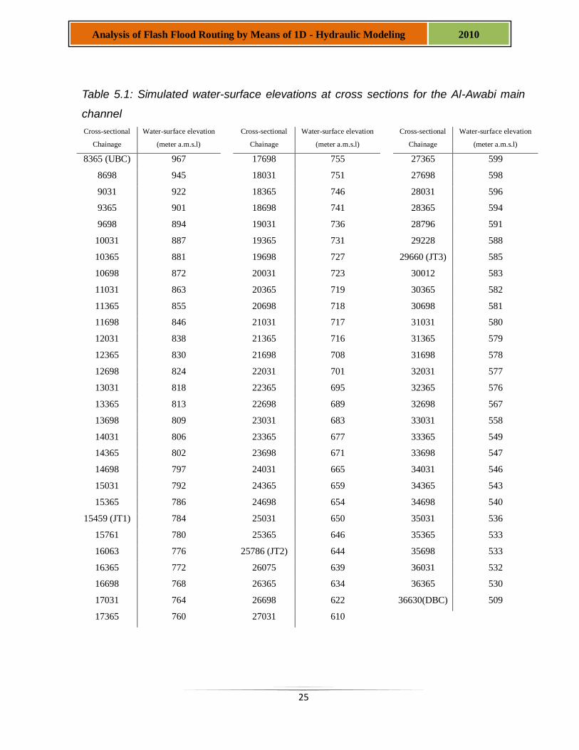
Table 5.1: Simulated water-surface elevations at cross sections for the Al-Awabi main
channel ......................................................................................................................... 25
Table 5.2: Variation of simulated discharge in m^3/s on March 01, 2005 with different
Manning’s-M roughness coefficient ............................................................................... 28
Table 5.3: Comparison of partial rainfall coverage on simulated water-depth ............... 41
x
Analysis of Flash Flood Routing by Means of 1D - Hydraulic Modeling 2010
Acronyms
a.m.s.l Above mean sea level
Arc GIS Software for Geographic Information Systems
ASTER - DEM Advanced Spaceborne Thermal Emission and
Reflection Radiometer - DEM
BC Boundary Condition
DBC Downstream Boundary Condition
DEM Digital Elevation Model
DHI Danish Hydraulic Institute
DHI WASY GmbH DHI WASY GmbH represents the group in Germany,
Austria and German-speaking Switzerland and is a
center of excellence in ground water for the entire DHI
group.
DS Down Stream
ESRI Environmental Systems Research Institute
FRM Flood Risk Management
GIS Geographic Information System
GDEM Global Digital Elevation Model
Google Earth It is a virtual globe, map, and geographic information
computer model by Google company.
GWL Ground Water Leakage; and it defines the leakage
coefficient to the loss of water from the Wadi channel
flow.
HD Hydrodynamic
i.e. That is
METI Ministry of Economy, Trade, and Industry
MIKE 11 Professional software package for 1D simulation of
flows in rivers and channels.
MIKE GIS / MIKE 11 GIS MIKE software with an extension to Arc GIS
MIKE NAM or MIKE RR Hydrological model to simulate runoff from the rainfall &
xi
Analysis of Flash Flood Routing by Means of 1D - Hydraulic Modeling 2010
NAM stands for Nedbor Afstromnings Model in Danish
language; whereas RR stands for rainfall-Runoff.
MIKE View Viewing software used to view MIKE 11 model results
MIKE Zero MIKE Zero is a software informer developed by DHI
which gives access to DHI’s modeling system.
NASA United States National Aeronautics and Space
Administration
RASTER DEM Data structure where the geographic area is divided into
cells i.e. row and column.
UBC Upstream Boundary Condition
US Up Stream
1D-Hydraulic Model One Dimensional Hydraulic Model
3D Three Dimensional
1
Analysis of Flash Flood Routing by Means of 1D - Hydraulic Modeling 2010
1. Introduction
This chapter introduces a distributed meso-scale catchment modelling of flood routing
and addresses the research challenges, objectives and potentiality of the distributed
catchment model of Al-Awabi watershed area located at the mountainous area of
Batinah Region of the Sultanate of Oman. It also provides a brief relevant literature
background typically utilized for executing and analyzing the overall tasks within the
scope and motivation of this study work.
1.1 Problem Statement
Arid areas such as Oman are typically characterized with both extremes of hydrological
events that are drought and flood. Due to this extreme nature of rainfall – runoff events,
and an inadequate or no existing coping mechanism measures and structures
implemented; a natural disaster such as flash flood has been a common phenomenon
in the Batinah region of the sultanate of Oman. Thus, in this study area, flash flooding is
the major problem.
Channel cross-sections are one of the main inputs to the 1D-Hydraulic Model used for
the analysis of flash flood routing. Whereas, field measurements of the Wadi channel
cross-sections are labor intensive and expensive activities. Thus, availability of
measured channel cross-sections is barely found in this study area; thereby making it
difficult to simulate the flood water level and discharge using MIKE 11 HD. Moreover,
uncertainty in channel geometry, roughness, and a flow description are highly
anticipated to impact on the sensitivity analysis of the model.
For these reasons, flash flood routing technique should be developed and analyzed
continuously so as to prevent any of such effects. However, since there are a lot of
uncertainties on the estimated data, roughness and geometry of channel, transmission
losses and vegetation covers, analysis is not an easy process. Data necessary for
carrying out routing analysis is very limited in the study area. Thus, to bridge these data
gaps, a methodology of gathering information from the ASTER DEM (27mX27m),
Google Earth maps, and Russian topographic maps is to be used in order to assess the
2
Analysis of Flash Flood Routing by Means of 1D - Hydraulic Modeling 2010
topographic nature of the watershed surface and the network of the Wadi channel
networks.
Therefore, the above reputed problems will be overcome from this research work when
carefully studied over the key and controlling model parameters.
1.2 Research Objectives
In view of the above stated shortcomings, derivation and processing of these flood
routing parameters by means of 1D-Hydraulic Modeling i.e. MIKE 11 HD is expected to
contribute to an overall comprehension of the sensitivity and scenario analysis of the
flash flood routing in Al-Awabi watershed area, and reliable estimation of hydrological
and hydraulic characteristics. With the aid of GIS-supported assessment, analysis
capability will be enhanced with regard to sub-watersheds topology, querying, display
and mapping of results, in other words making the analysis process at the finger tips of
the end user.
The ultimate goal of this study work will serve as a catchment modeling tool that
investigate both the uncertainties in flash flood routing analysis based on limited data
and distinct characteristics of rainfall-runoff-processes in the study area; for instance,
partial area coverage of rainfall and transmission losses. And this goal will be achieved
by performing and executing the following tasks accordingly i.e. the 1D-Hydraulic model
setup for the target watershed of Al-Awabi i.e. MIKE 11 HD; sensitivity analysis;
scenario analysis on impacts of rainfall characteristics; and finally working on the overall
discussion of results.
1.3 Research Potentiality
This study work is an essential part of the distributed meso-scale catchment modelling,
and the setup of a 1D – Hydraulic Model based on available data shall support the
development of the distributed catchment model of Al-Awabi watershed. It will further
have its contribution to the ultimate goal of the water balance assessment work in that
region via replication of the process both temporally and spatially. Furthermore, as
3
Analysis of Flash Flood Routing by Means of 1D - Hydraulic Modeling 2010
partnership using the watershed approach, this study work will serve as a corner
foundation stone towards the complete catchment-scale model which consists of hill-
slope surface and channel flow sub-models coupled together in one comprehensive
model to account for catchment rainfall-runoff production and flood routing applicable to
flood transmission losses in the mountainous area of the Batinah region, Oman.
1.4 Overview of Relevant Literature Review
1.4.1 Overview of GIS
Networks can be easily analyzed and assessed if there is an interaction between
databases and maps; and this is why the Geographic Information System (GIS) comes
to an application. GIS is an information system that answers questions from a database
of spatially distributed features and procedures to collect, store, retrieve, analyze and
display geographic data (Shamsi, 2005). GIS helps professionals in mapping,
monitoring, modeling and maintenance of water related systems. Thus, by doing so, a
considerable time and money is saved. GIS users benefit from the GIS’s easier and
quicker results in analyzing problems and recommending solutions within a fraction of
the time otherwise that would be required with a tedious manual working means.
1.4.2 Digital Elevation Models
Digital Elevation Models (DEM) also called digital terrain models provide a 3D
representation of the real-world topography. DEM creation requires data collection and
processing procedures. Data collection step depends on the areal extent and
importance of the study. They can be constructed by ordinary ground survey when the
study area is relatively small or of minor importance. On the other hand if the study area
is large, satellites can be used for mapping the topography. These maps then have to
be processed by remote sensing imagery to give topographic elevation information. This
is how the DEMs covering the entire globe, for example, the Advanced Spaceborne
Thermal Emission and Reflection Radiometer (ASTER) Global Digital Elevation Model
(GDEM) which was developed jointly by the Ministry of Economy, Trade, and Industry
(METI) of Japan and the United States National Aeronautics and Space Administration
(NASA) are formed.
4
Analysis of Flash Flood Routing by Means of 1D - Hydraulic Modeling 2010
DEMs have vital role in hydrological analysis especially in delineating watersheds,
obtaining stream network, and related analysis. The accuracy of the stream network
obtained from DEMs is highly dependent on the resolution of the DEM. For instance, the
ASTER GDEM tiles (1◦×1◦tiles) of resolution 27m×27m were downloaded from the
website of ASTER GDEM (GDEM, 2009), and the DEM tiles were made mosaic to get
the complete DEM of the Al-Awabi watershed area.
1.4.3 Applications of GIS in Hydrology
Hydrological applications of GIS are extremely varied. Whilst hydrological scientists
have progressed in their representations of hydrological processes from lumped through
semi-distributed to distributed hydrological models, water resource managers have
followed a parallel route in the increasing spatial resolution with which assets,
particularly infrastructure, have been represented, interrelated and managed
(Garbrecht, 2000). With the increasing availability of high-resolution DEMs such as
ASTER DEM (27m×27m), the most widespread application of GIS in hydrology is the
identification of drainage pathways and runoff contributing areas based on topographic
form, and their coupling with hydrological and hydraulic models, for example MIKE NAM
and MIKE 11 HD.
Although catchment-scale hydrological modeling represents an important GIS
application within hydrology, GIS has relevance to the solution of many other
hydrological problems at local, catchment and regional scales. And the same is also
true with this study work’s GIS utilization.
1.4.4 Flood Routing
Also called streamflow routing and channel routing, is one of the classical problems in
applied hydrology. The word routing refers in general to the mathematical procedure of
tracking or following water movement from one place to another; as such, the word also
includes the description of the conversion of precipitation into various subsurface and
surface runoff phenomena. However, flood routing refers specifically to the description
5
Analysis of Flash Flood Routing by Means of 1D - Hydraulic Modeling 2010
of the behavior of a flood wave as it moves along in a well defined open channel
(Brutsaert, 2005). The wave, to be dealt in this study area, is typically the result of
inflows into the Wadi channel following heavy rainfall. For the routing of a flood wave,
numerical methods that solve the complete continuity and momentum equations may be
used.
Fully Dynamic: It is an HD Module which provides fully dynamic solution to the
complete nonlinear Saint Venant equations for an open channel flow.
Kinematic Models: These models are based on the solution of the continuity
equation and the steady-uniform equation for the dynamic equation. The waves
propagated using these models are called kinematic waves, and routing is called
kinematic routing.
Diffusion Routing: This is formulated based on the simplified versions of
momentum equation.
Muskingum-Cunge Method: This method is actually a particular finite-difference
approximation of the kinematic wave equations and present expressions for the
Muskingum coefficients in terms of the physical properties of the channel. And
the coefficients for the method were determined from the observed flood records.
1.4.5 MIKE 11 Hydrodynamic Models
MIKE 11HD model is a one-dimensional hydraulic modeling software package,
developed at Danish Hydraulic Institute in 1987. The model has been widely used to
simulate water levels and flow in the river systems. It has an interface to GIS allowing
for preparation of model input and presentation of model output in a GIS environment, in
which this study work was conducted using this package called MIKE11 GIS. It merges
the technologies of hydraulic modeling, MIKE 11, and Arc GIS developed by ESRI. This
is designed to run into Arc GIS environment which can automatically integrate water
level resulting from MIKE11-HD into digital elevation map (DEM) for which we can
determine the inundated area at the rainfall-runoff events within the study area.
6
Analysis of Flash Flood Routing by Means of 1D - Hydraulic Modeling 2010
2. Study Area and data
2.1 Study area
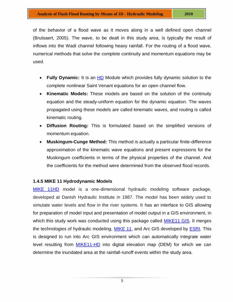
This study was conducted at the mountainous catchment part of Batinah Region of the
Sultanate of Oman called Al-Awabi watershed which is about 260km2 in area (Figure
2.1). Oman is known as one of the world’s arid areas. It is located in the southeast of
the Arabian Peninsula. It is bordered by Saudi Arabia to the west, United Arab Emirates
to the northwest, Yemen to the south east and Arabian Sea to the east.
Figure 2.1: Al-Awabi watershed area location with respect to Oman (Google Earth map)
Among the flood events which took place in Oman, almost all are categorized as flash
floods. Oman is characterized by arid and/or semi arid climatic conditions, with many
periods of drought followed by few periods of convective or advective rainstorms
typically intense and erratic rainfalls produced in short time. Flash flooding can cause
severe damage to buildings and infrastructures and pose a high risk to life and
properties. And it is naturally very difficult to model and forecast bearing in mind the lack
7
Analysis of Flash Flood Routing by Means of 1D - Hydraulic Modeling 2010
of enough data and sustainable working system in the target area, Al-Awabi watershed,
Batinah region, Oman.
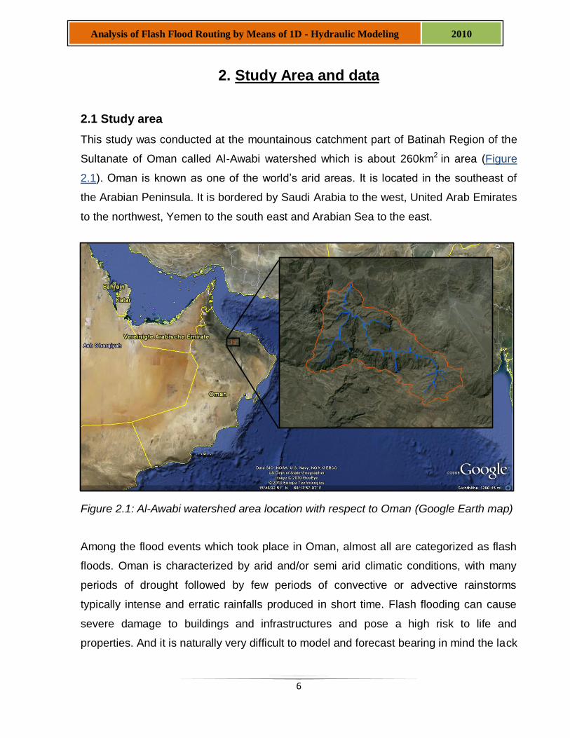
2.1.1 Target Watershed Area
The study area i.e. Al-Awabi watershed is located at the northern escarpment part of
Oman, south of Batinah region and is one of the main tributaries to Wadi Bani-Kharus. It
is situated at the south of the whole Bani-Kharus catchment area. Furthermore, the
DEM and channel network within the Al-Awabi watershed as depicted in Figure 2.2 was
generated from ASTER DEM using Arc GIS; and the given watershed was described as
third order stream that is a tributary formed by two or more second order streams as
well as streams of lower order.
Figure 2.2: Al-Awabi watershed area
The watershed lies between latitude 2555187 to 2576337 and longitude 545997 to
573706. The total area is 254 km2 with a major portion of it is mountainous area and
lays in the south of Batinah Region with a surface area and volume of about 300km2
and 235km3 respectively as shown in Figure 2.3. Within the watershed, there is one
8
Analysis of Flash Flood Routing by Means of 1D - Hydraulic Modeling 2010
runoff gauge which is located at latitude of 23o17’47” and longitude of 57o31’43” (Table
2.1).
Table 2.1: Location of Study Area-Runoff Gauge
Station Name Latitude Longitude Watershed Tributary Area Region Elevation
Awabi near Awabi 23°17’47” 57°31’43” Al-Awabi Bani Kharus 254Km^2 South Batinah 500m
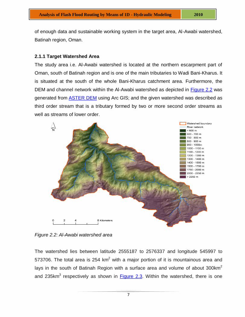
The average surface elevation of the watershed area ranges from 496 m to 2483 m
a.m.s.l. with a mean slope of about 25o. The area being almost ragged mountainous,
there was severe flash flood occurrence at downstream of the watershed and its vicinity
during heavy rainfall events. The hill-shade and slope of the Al-Awabi watershed were
generated and shown in Figure 2.3 for better visualization of the ground surface.
Figure 2.3: Al-Awabi Watershed Hill-shade (left) and Slope (right)
2.2 Data
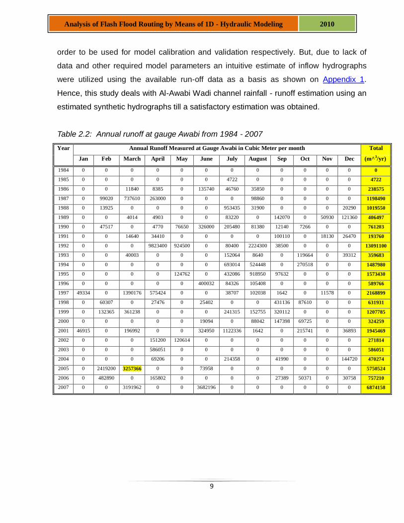
Daily runoff data at Awabi gauging site for a period of 23 years (1984–2007) was
recorded and analyzed as shown in Table 2.2. For the hydraulic model set-up, water
level and channel cross-section data are required; hence, based on the available runoff
data an estimated inflow hydrograph was tried to be generated using MIKE NAM in
9
Analysis of Flash Flood Routing by Means of 1D - Hydraulic Modeling 2010
order to be used for model calibration and validation respectively. But, due to lack of
data and other required model parameters an intuitive estimate of inflow hydrographs
were utilized using the available run-off data as a basis as shown on Appendix 1.
Hence, this study deals with Al-Awabi Wadi channel rainfall - runoff estimation using an
estimated synthetic hydrographs till a satisfactory estimation was obtained.
Table 2.2: Annual runoff at gauge Awabi from 1984 - 2007
Year Annual Runoff Measured at Gauge Awabi in Cubic Meter per month Total
Jan Feb March April May June July August Sep Oct Nov Dec (m^3/yr)
1984 0 0 0 0 0 0 0 0 0 0 0 0 0
1985 0 0 0 0 0 0 4722 0 0 0 0 0 4722
1986 0 0 11840 8385 0 135740 46760 35850 0 0 0 0 238575
1987 0 99020 737610 263000 0 0 0 98860 0 0 0 0 1198490
1988 0 13925 0 0 0 0 953435 31900 0 0 0 20290 1019550
1989 0 0 4014 4903 0 0 83220 0 142070 0 50930 121360 406497
1990 0 47517 0 4770 76650 326000 205480 81380 12140 7266 0 0 761203
1991 0 0 14640 34410 0 0 0 0 100110 0 18130 26470 193760
1992 0 0 0 9823400 924500 0 80400 2224300 38500 0 0 0 13091100
1993 0 0 40003 0 0 0 152064 8640 0 119664 0 39312 359683
1994 0 0 0 0 0 0 693014 524448 0 270518 0 0 1487980
1995 0 0 0 0 124762 0 432086 918950 97632 0 0 0 1573430
1996 0 0 0 0 0 400032 84326 105408 0 0 0 0 589766
1997 49334 0 1390176 575424 0 0 38707 102038 1642 0 11578 0 2168899
1998 0 60307 0 27476 0 25402 0 0 431136 87610 0 0 631931
1999 0 132365 361238 0 0 0 241315 152755 320112 0 0 0 1207785
2000 0 0 0 0 0 19094 0 88042 147398 69725 0 0 324259
2001 46915 0 196992 0 0 324950 1122336 1642 0 215741 0 36893 1945469
2002 0 0 0 151200 120614 0 0 0 0 0 0 0 271814
2003 0 0 0 586051 0 0 0 0 0 0 0 0 586051
2004 0 0 0 69206 0 0 214358 0 41990 0 0 144720 470274
2005 0 2419200 3257366 0 0 73958 0 0 0 0 0 0 5750524
2006 0 482890 0 165802 0 0 0 0 27389 50371 0 30758 757210
2007 0 0 3191962 0 0 3682196 0 0 0 0 0 0 6874158
10
Analysis of Flash Flood Routing by Means of 1D - Hydraulic Modeling 2010
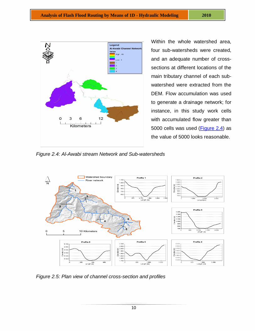
Within the whole watershed area,
four sub-watersheds were created,
and an adequate number of cross-
sections at different locations of the
main tributary channel of each sub-
watershed were extracted from the
DEM. Flow accumulation was used
to generate a drainage network; for
instance, in this study work cells
with accumulated flow greater than
5000 cells was used (Figure 2.4) as
the value of 5000 looks reasonable.
Figure 2.4: Al-Awabi stream Network and Sub-watersheds
Figure 2.5: Plan view of channel cross-section and profiles
11
Analysis of Flash Flood Routing by Means of 1D - Hydraulic Modeling 2010
Six cross-sections at different channel locations of the selected sub-watersheds were
identified and extracted from the DEM of Al-Awabi watershed as shown in Figure 2.5
using Arc GIS for demonstration purpose otherwise numerous number of cross-sections
had been extracted using MIKE GIS and were modified during model setup as
described in section 4.
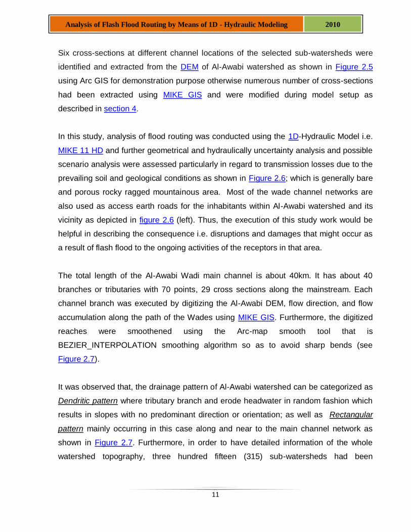
In this study, analysis of flood routing was conducted using the 1D-Hydraulic Model i.e.
MIKE 11 HD and further geometrical and hydraulically uncertainty analysis and possible
scenario analysis were assessed particularly in regard to transmission losses due to the
prevailing soil and geological conditions as shown in Figure 2.6; which is generally bare
and porous rocky ragged mountainous area. Most of the wade channel networks are
also used as access earth roads for the inhabitants within Al-Awabi watershed and its
vicinity as depicted in figure 2.6 (left). Thus, the execution of this study work would be
helpful in describing the consequence i.e. disruptions and damages that might occur as
a result of flash flood to the ongoing activities of the receptors in that area.
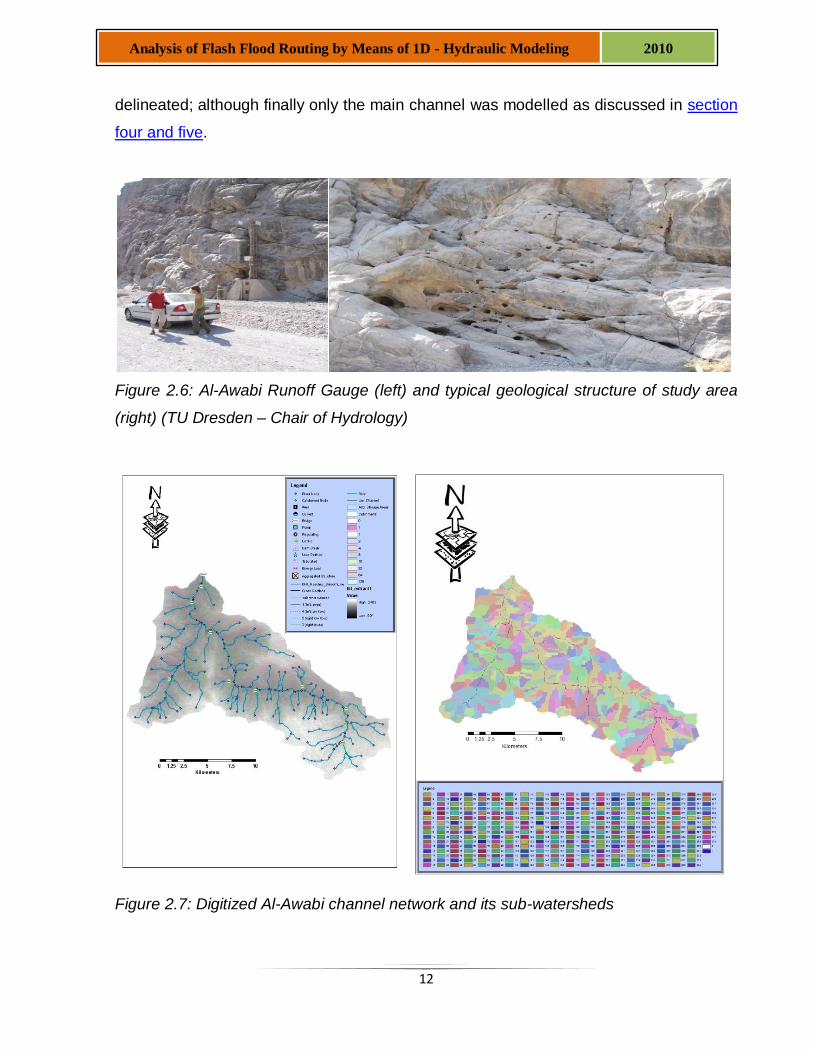
The total length of the Al-Awabi Wadi main channel is about 40km. It has about 40
branches or tributaries with 70 points, 29 cross sections along the mainstream. Each
channel branch was executed by digitizing the Al-Awabi DEM, flow direction, and flow
accumulation along the path of the Wades using MIKE GIS. Furthermore, the digitized
reaches were smoothened using the Arc-map smooth tool that is
BEZIER_INTERPOLATION smoothing algorithm so as to avoid sharp bends (see
Figure 2.7).
It was observed that, the drainage pattern of Al-Awabi watershed can be categorized as
Dendritic pattern where tributary branch and erode headwater in random fashion which
results in slopes with no predominant direction or orientation; as well as Rectangular
pattern mainly occurring in this case along and near to the main channel network as
shown in Figure 2.7. Furthermore, in order to have detailed information of the whole
watershed topography, three hundred fifteen (315) sub-watersheds had been
12
Analysis of Flash Flood Routing by Means of 1D - Hydraulic Modeling 2010
delineated; although finally only the main channel was modelled as discussed in section
four and five.
Figure 2.6: Al-Awabi Runoff Gauge (left) and typical geological structure of study area
(right) (TU Dresden – Chair of Hydrology)
Figure 2.7: Digitized Al-Awabi channel network and its sub-watersheds
13
Analysis of Flash Flood Routing by Means of 1D - Hydraulic Modeling 2010
3. Research Methodology
3.1 Overall Scheme
A good starting point for a quantitative assessment of runoff is to consider the physical
processes occurring in the hydrological cycle of the study area. And from this, a set of
influencing factors could be proposed which determine the response of the watershed to
rainfall; namely, watershed area, soil type and depth, channel and surface slopes, rock
type and area, vegetation cover, reservoirs, sealed areas if available and so on of the
study area. Therefore, in this study work, we are dealing with Wadi channel routing
problem i.e. to find the outflow hydrograph from the Wadi river reach from the inflow
hydrograph. And MIKE 11 HD was used for this study work.
Furthermore, as in many practical situations, no historical time series of inflow-outflow
data were available for the Al-Awabi watershed area. Hence, the model must be
synthesized from physical information on the system available from the topographical
map, Google Earth map, and/or from RASTER DEMs. Therefore, it would be highly
desirable to find a linkage between physically sound hydrodynamic models and
hydrological conceptual models.
3.2 Task-1: Model setup for Al-Awabi watershed area
This first task comprises the relevant data assimilation and estimation, and setup of 1D-
Hydroulic modeling i.e. MIKE 11 HD, the model applied to assess the flash flood routing
analysis within the Al-Awabi watershed area. Hence, this task comprises the following
sub-tasks:
Derivation of sub watersheds and/or channel network using Arc GIS or MIKE GIS
for the Al-Awabi watershed based on ASTER-DEM (27X27m).
Digitization of cross-section at decisive stations of the longitudinal sections based
on ASTER-DEM (27x27m), and Google Earth map.
Setup of the 1D-Hydraulic model that is MIKE 11HD.
14
Analysis of Flash Flood Routing by Means of 1D - Hydraulic Modeling 2010
3.3 Task-2: Sensitivity Analysis
It was the task of this paper to make a sensitivity analysis of as to how and to what
degree the variation of model input affects the output uncertainty particularly in regard to
the following factors:
Preparation of upper boundaries (inflow) –based on reasonable assumptions.
Impacts of uncertainties in channel geometry.
Impacts of uncertainties in channel roughness.
Impacts of numerical flow descriptions.
3.4 Task-3: Scenario analysis
Scenario analysis is defined as a process of analyzing possible future events by
considering alternative possible outcomes. Thus, this study work focuses on two main
Scenarios analyzed on the target watershed.
Scenario analysis considering the partial area coverage of rainfall.
Scenario analysis considering transmission losses.
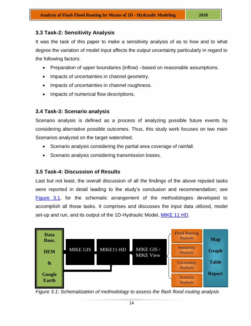
3.5 Task-4: Discussion of Results
Last but not least, the overall discussion of all the findings of the above reputed tasks
were reported in detail leading to the study’s conclusion and recommendation; see
Figure 3.1, for the schematic arrangement of the methodologies developed to
accomplish all those tasks. It comprises and discusses the input data utilized, model
set-up and run, and its output of the 1D-Hydraulic Model, MIKE 11 HD.
Figure 3.1: Schematization of methodology to assess the flash flood routing analysis
Data
Base,
DEM
&
Earth
Flood Routing
Analysis
Map
Graph
Table
Report
Sensitivity
Analysis
Routing
Analysis Uncertainty
Analysis
Scenario
Analysis
MIKE GIS
MIKE11-HD
MIKE GIS /
MIKE View
15
Analysis of Flash Flood Routing by Means of 1D - Hydraulic Modeling 2010
4. ASTER DEM and Hydro Dynamic Model Set up
4.1 ASTER DEM and Digitization of MIKE GIS
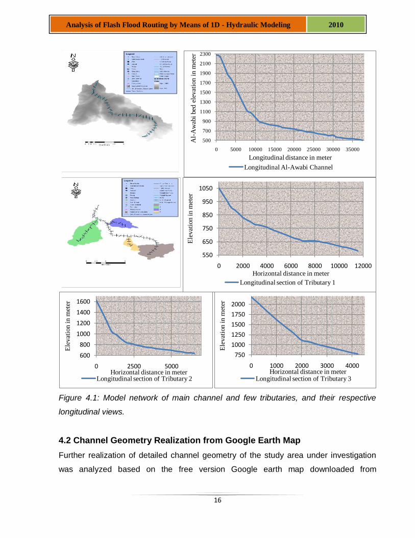
As mentioned in section one, an ASTER DEM for Al-Awabi watershed was extracted
using Arc GIS 9.3 and digitization of the respected channel network and cross-section
were executed using the MIKE 11 GIS as shown in Figure 4.1. Furthermore, data error
analysis and modification of extracted channel cross-sections had been dealt by doing a
comparison work for the processed DEM that was digitized in MIKE GIS with that of
cross-sections derived from Google Earth.
Putting into consideration the MIKE 11 simulation requirement, and the limited data
availability, this study work focuses at analyzing for a well selected and quite
representative four sub-watersheds which are distributed spatially within Al-Awabi
watershed so as to meet the study’s overall task. Furthermore, although the whole
watershed is a mountainous ragged area, relatively speaking, the whole main channel
bed slope can be categorized into three divisions such as: chainage 0 to 10,000: flat
bed slope; chainage 10,000 to 25,000: gentle bed slope; and chainage 25,000 to
37,690: steep bed slope. (See the longitudinal profile section of the Al-Awabi main
channel in Figure 4.1).
16
Analysis of Flash Flood Routing by Means of 1D - Hydraulic Modeling 2010
Figure 4.1: Model network of main channel and few tributaries, and their respective
longitudinal views.
4.2 Channel Geometry Realization from Google Earth Map
Further realization of detailed channel geometry of the study area under investigation
was analyzed based on the free version Google earth map downloaded from
500
700
900
1100
1300
1500
1700
1900
2100
2300
0 5000 10000 15000 20000 25000 30000 35000
Al-
Aw
abi
bed
ele
vat
ion
in
met
er
Longitudinal distance in meter
Longitudinal Al-Awabi Channel
550
650
750
850
950
1050
0 2000 4000 6000 8000 10000 12000
Ele
vat
ion
in
met
er
Horizontal distance in meter
Longitudinal section of Tributary 1
600
800
1000
1200
1400
1600
0 2500 5000
Ele
vat
ion
in
met
er
Horizontal distance in meterLongitudinal section of Tributary 2
750
1000
1250
1500
1750
2000
0 1000 2000 3000 4000
Ele
vat
ion
in
met
er
Horizontal distance in meterLongitudinal section of Tributary 3
17
Analysis of Flash Flood Routing by Means of 1D - Hydraulic Modeling 2010
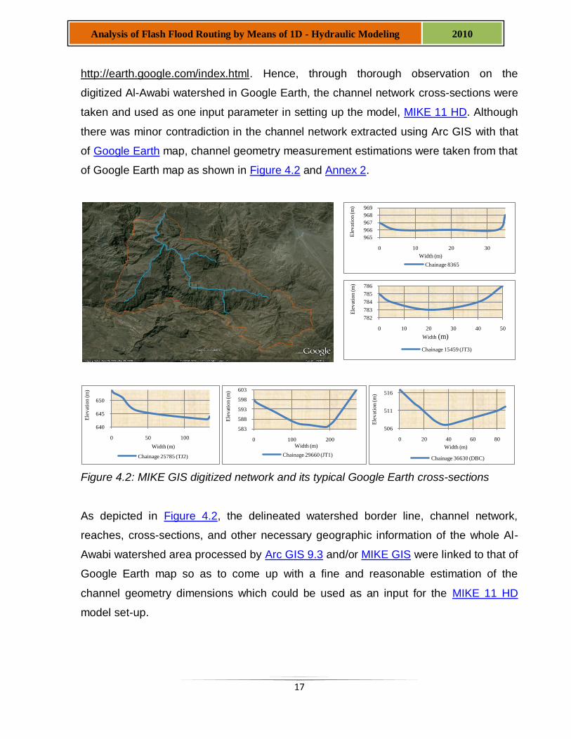
http://earth.google.com/index.html. Hence, through thorough observation on the
digitized Al-Awabi watershed in Google Earth, the channel network cross-sections were
taken and used as one input parameter in setting up the model, MIKE 11 HD. Although
there was minor contradiction in the channel network extracted using Arc GIS with that
of Google Earth map, channel geometry measurement estimations were taken from that
of Google Earth map as shown in Figure 4.2 and Annex 2.
Figure 4.2: MIKE GIS digitized network and its typical Google Earth cross-sections
As depicted in Figure 4.2, the delineated watershed border line, channel network,
reaches, cross-sections, and other necessary geographic information of the whole Al-
Awabi watershed area processed by Arc GIS 9.3 and/or MIKE GIS were linked to that of
Google Earth map so as to come up with a fine and reasonable estimation of the
channel geometry dimensions which could be used as an input for the MIKE 11 HD
model set-up.
965
966
967
968
969
0 10 20 30
Ele
vat
ion
(m
)
Width (m)
Chainage 8365
782
783
784
785
786
0 10 20 30 40 50
Ele
vat
ion
(m
)
Width (m)
Chainage 15459 (JT3)
640
645
650
0 50 100
Ele
vat
ion
(m
)
Width (m)
Chainage 25785 (TJ2)
583
588
593
598
603
0 100 200
Ele
vat
ion
(m
)
Width (m)
Chainage 29660 (JT1)
506
511
516
0 20 40 60 80
Ele
vat
ion
(m
)
Width (m)
Chainage 36630 (DBC)
18
Analysis of Flash Flood Routing by Means of 1D - Hydraulic Modeling 2010
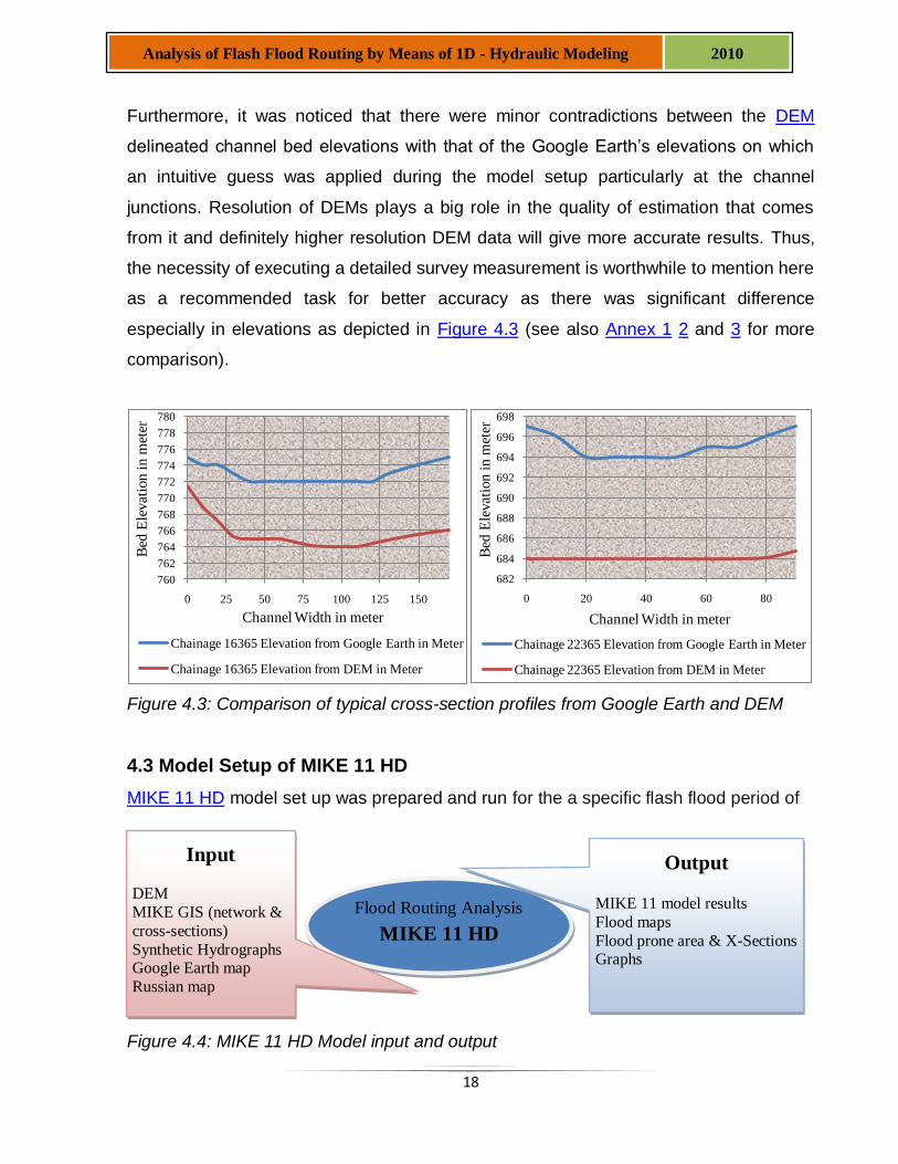
Furthermore, it was noticed that there were minor contradictions between the DEM
delineated channel bed elevations with that of the Google Earth’s elevations on which
an intuitive guess was applied during the model setup particularly at the channel
junctions. Resolution of DEMs plays a big role in the quality of estimation that comes
from it and definitely higher resolution DEM data will give more accurate results. Thus,
the necessity of executing a detailed survey measurement is worthwhile to mention here
as a recommended task for better accuracy as there was significant difference
especially in elevations as depicted in Figure 4.3 (see also Annex 1 2 and 3 for more
comparison).
Figure 4.3: Comparison of typical cross-section profiles from Google Earth and DEM
4.3 Model Setup of MIKE 11 HD
MIKE 11 HD model set up was prepared and run for the a specific flash flood period of
Figure 4.4: MIKE 11 HD Model input and output
760
762
764
766
768
770
772
774
776
778
780
0 25 50 75 100 125 150
Bed
Ele
vat
ion
in
met
er
Channel Width in meter
Chainage 16365 Elevation from Google Earth in Meter
Chainage 16365 Elevation from DEM in Meter
682
684
686
688
690
692
694
696
698
0 20 40 60 80
Bed
Ele
vat
ion
in
met
er
Channel Width in meter
Chainage 22365 Elevation from Google Earth in Meter
Chainage 22365 Elevation from DEM in Meter
Flood Routing Analysis
MIKE 11 HD
Output MIKE 11 model results
Flood maps
Flood prone area & X-Sections Graphs
Input DEM
MIKE GIS (network &
cross-sections)
Synthetic Hydrographs Google Earth map
Russian map
19
Analysis of Flash Flood Routing by Means of 1D - Hydraulic Modeling 2010
March in 2005 to simulate water level and discharge at different cross-sections of the
channel reaches within the Al-Awabi watershed area. The input and output of the MIKE
11 HD conducted and executed in this study work is depicted in Figure 4.4.
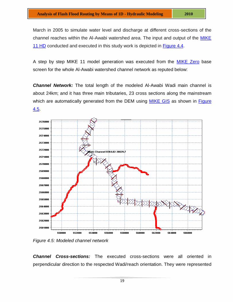
A step by step MIKE 11 model generation was executed from the MIKE Zero base
screen for the whole Al-Awabi watershed channel network as reputed below:
Channel Network: The total length of the modeled Al-Awabi Wadi main channel is
about 24km; and it has three main tributaries, 23 cross sections along the mainstream
which are automatically generated from the DEM using MIKE GIS as shown in Figure
4.5.
Figure 4.5: Modeled channel network
Channel Cross-sections: The executed cross-sections were all oriented in
perpendicular direction to the respected Wadi/reach orientation. They were represented
20
Analysis of Flash Flood Routing by Means of 1D - Hydraulic Modeling 2010
in two dimensional coordinates, namely, the transverse distance from a fixed point
represented in the abscissa (X - coordinate) and the channel bed elevation represented
in the Ordinate (Z - coordinate); and were automatically generated using MIKE GIS
which in turn further compared and checked for channel geometry dimensions from that
of Google Earth map as shown in Figure 4.5.
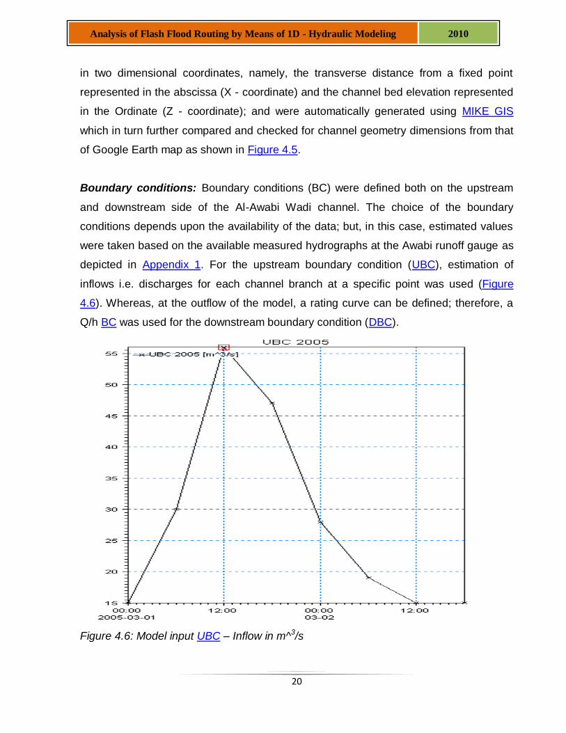
Boundary conditions: Boundary conditions (BC) were defined both on the upstream
and downstream side of the Al-Awabi Wadi channel. The choice of the boundary
conditions depends upon the availability of the data; but, in this case, estimated values
were taken based on the available measured hydrographs at the Awabi runoff gauge as
depicted in Appendix 1. For the upstream boundary condition (UBC), estimation of
inflows i.e. discharges for each channel branch at a specific point was used (Figure
4.6). Whereas, at the outflow of the model, a rating curve can be defined; therefore, a
Q/h BC was used for the downstream boundary condition (DBC).
Figure 4.6: Model input UBC – Inflow in m^3/s
21
Analysis of Flash Flood Routing by Means of 1D - Hydraulic Modeling 2010
Hydrodynamic parameters: Global initial conditions in the Wadi flow, Bed Resistance
and wave approximation were set for the HD calculations. The fully dynamic wave
approximation method was used for the simulation of the Wade flow in order to
conserve both momentum and continuity in the calculation as it might not be possible to
use the diffusive wave approach because the whole Awabi channel bed was rather
steep in most of the branches and flow may become super-critical at several points.
And, the initial bed resistance value based on the Manning co-efficient, M (M = 1/n,
where n is Manning’s coefficient) was set to 20, 30 and 40. Whereas, initial water depth
of 0.003m was specified; and discharge was also set to 15m3/s so as to avoid the drying
out of the flow channel.
Simulation: Last but not least, model simulation was done using the unsteady
simulation mode of the HD model for the flash flood Wade flow within Al-Awabi
watershed. It was simulated for the period of time on March 1st at 00:00 to 2nd at 18:00
in 2005 for a simulation time step of 30 seconds. Furthermore, a Hotstart file type of
condition that is the initial conditions were loaded from an existing result file that was
executed using the quasi steady simulation mode.
22
Analysis of Flash Flood Routing by Means of 1D - Hydraulic Modeling 2010
5. Results and Discussions
5.1 Flood Routing using 1D-Hydraulic Model
The model set up of MIKE 11 HD for the flash flood routing of Al-Awabi Wadi was one of
the most important application of free surface water flows in ephemeral rivers. Hence,
the modules applied to analyze the flash flood routing for the selected watershed
includes the module HD in MIKE11 which was responsible to simulate the hydraulic
regimes including water level, and discharge along the channel. In this study paper,
MIKE NAM was not used due to unavailability of required data; instead, an estimated
inflow hydrograph was used that was derived based on the recorded output hydrograph.
Therefore, the model set here basically was MIKE 11 HD; where the channel network
and cross-sections were generated using the MIKE GIS and exported to MIKE 11
network and cross-section editors; while BC, HD parameters, and simulation were
performed in MIKE 11. Finally, the executed simulation results were viewed via MIKE
View and/or MIKE GIS.
5.1.1 Model Cross-section - Hydraulic Parameters
The cross-section hydraulic parameters were computed automatically at different stages
for the estimated and/or DEM extracted cross-sections along the digitized channel
network of Al-Awabi watershed. An open section type and Resistance Radius were
chosen for the channel cross-section settings. In addition, a bed slope was computed
automatically from the cross-section data executed by setting the datum function. The
bed resistance of the cross-sections in this study work was described using the three
transversal distribution options given in MIKE 11 that is Uniform, High/Low flow zones,
and Distributed where the uniform one was used during the model set up.
Furthermore, the Manning’s - n runoff coefficient of the Al-Awabi Wadi was estimated to
be within the range of 0.025 to 0.05; and the corresponding values for M are from 40 to
20. The Chezy coefficient, C, is related to Manning's n in terms of hydraulic radius, R,
as: and was determined during model calibration accordingly.
23
Analysis of Flash Flood Routing by Means of 1D - Hydraulic Modeling 2010
5.1.2 Calibration of MIKE 11 HD Model
MIKE 11 HD model set up was prepared and run for the period of time on March 1st at
00:00 to March 2nd at 18:00 in 2005 to simulate water level and discharge at different
cross-sections of the channel reach within the Al-Awabi watershed area. For the UBC,
an estimated inflow was used; whereas, a rating curve Q/h BC was used for the DBC.
Manning’s roughness coefficient was taken as a model calibration parameter and its
value at different locations along the main channel was estimated while the GWL
coefficient was set to be zero. The simulation time step was set to 30 seconds and the
interval between consecutive computational grids was kept as 450 meter.
Furthermore, due to the topography of the Al-Awabi watershed and its rainfall intensity
and coverage, a flash flood occurs which makes the resulted runoff to be governed by
dynamic waves rather than the kinematic waves. Thus, the fully dynamic option was
used in this model work out of the three flow description module options such as
dynamic wave, diffusive wave, and kinematic wave approaches.
Finally, a modification work was applied to the channel cross-section during the model
setup particularly at the junctions of the tributaries due to discrepancies on the derived
bed elevations from respective channel braches with that of the main channel. It was
also observed that a significant impact to the modeled results as well as among each of
the corresponding digitized cross-sections which in turn make the model setup task very
complex. Thus, in order to overcome this instability and complexity in the model set up,
a DELTA value was altered from its default value 0.50 to 0.70 during calibration. And it
was noticed that changing the DELTA value i.e. a coefficient in HD parameter used to
dampen potential instabilities had a very significant impact to the model set up; whereas
almost no effect to the modeled results of this study paper as shown on Figure 5.1.
24
Analysis of Flash Flood Routing by Means of 1D - Hydraulic Modeling 2010
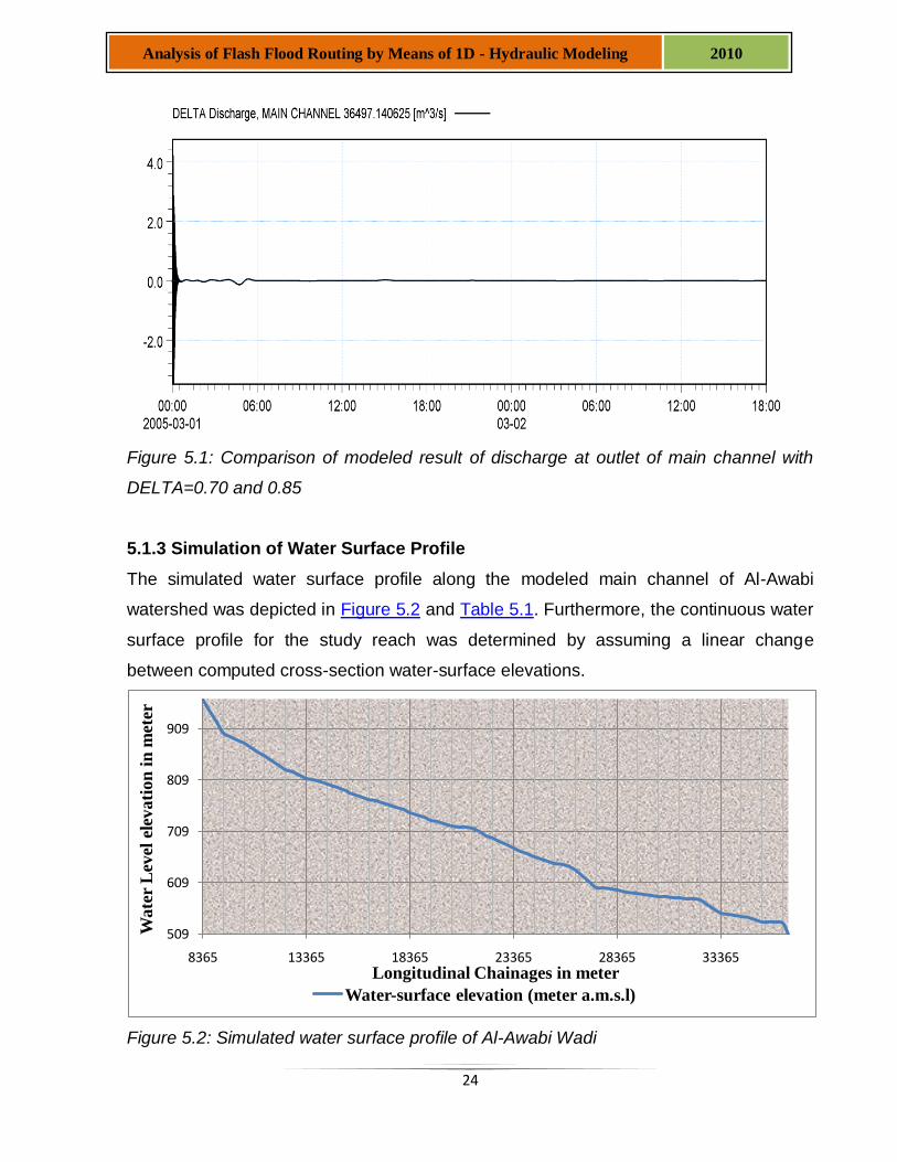
Figure 5.1: Comparison of modeled result of discharge at outlet of main channel with
DELTA=0.70 and 0.85
5.1.3 Simulation of Water Surface Profile
The simulated water surface profile along the modeled main channel of Al-Awabi
watershed was depicted in Figure 5.2 and Table 5.1. Furthermore, the continuous water
surface profile for the study reach was determined by assuming a linear change
between computed cross-section water-surface elevations.
Figure 5.2: Simulated water surface profile of Al-Awabi Wadi
509
609
709
809
909
8365 13365 18365 23365 28365 33365
Wate
r L
evel
ele
vati
on
in
met
er
Longitudinal Chainages in meter
Water-surface elevation (meter a.m.s.l)
25
Analysis of Flash Flood Routing by Means of 1D - Hydraulic Modeling 2010
Table 5.1: Simulated water-surface elevations at cross sections for the Al-Awabi main
channel
Cross-sectional
Chainage
Water-surface elevation
(meter a.m.s.l)
Cross-sectional
Chainage
Water-surface elevation
(meter a.m.s.l)
Cross-sectional
Chainage
Water-surface elevation
(meter a.m.s.l)
8365 (UBC) 967
17698 755
27365 599
8698 945
18031 751
27698 598
9031 922
18365 746
28031 596
9365 901
18698 741
28365 594
9698 894
19031 736
28796 591
10031 887
19365 731
29228 588
10365 881
19698 727
29660 (JT3) 585
10698 872
20031 723
30012 583
11031 863
20365 719
30365 582
11365 855
20698 718
30698 581
11698 846
21031 717
31031 580
12031 838
21365 716
31365 579
12365 830
21698 708
31698 578
12698 824
22031 701
32031 577
13031 818
22365 695
32365 576
13365 813
22698 689
32698 567
13698 809
23031 683
33031 558
14031 806
23365 677
33365 549
14365 802
23698 671
33698 547
14698 797
24031 665
34031 546
15031 792
24365 659
34365 543
15365 786
24698 654
34698 540
15459 (JT1) 784
25031 650
35031 536
15761 780
25365 646
35365 533
16063 776
25786 (JT2) 644
35698 533
16365 772
26075 639
36031 532
16698 768
26365 634
36365 530
17031 764
26698 622
36630(DBC) 509
17365 760
27031 610
26
Analysis of Flash Flood Routing by Means of 1D - Hydraulic Modeling 2010
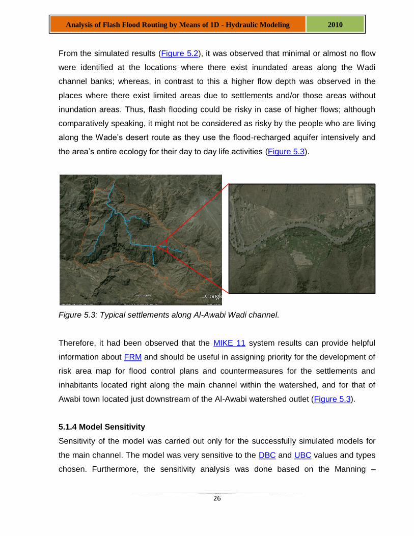
From the simulated results (Figure 5.2), it was observed that minimal or almost no flow
were identified at the locations where there exist inundated areas along the Wadi
channel banks; whereas, in contrast to this a higher flow depth was observed in the
places where there exist limited areas due to settlements and/or those areas without
inundation areas. Thus, flash flooding could be risky in case of higher flows; although
comparatively speaking, it might not be considered as risky by the people who are living
along the Wade’s desert route as they use the flood-recharged aquifer intensively and
the area’s entire ecology for their day to day life activities (Figure 5.3).
Figure 5.3: Typical settlements along Al-Awabi Wadi channel.
Therefore, it had been observed that the MIKE 11 system results can provide helpful
information about FRM and should be useful in assigning priority for the development of
risk area map for flood control plans and countermeasures for the settlements and
inhabitants located right along the main channel within the watershed, and for that of
Awabi town located just downstream of the Al-Awabi watershed outlet (Figure 5.3).
5.1.4 Model Sensitivity
Sensitivity of the model was carried out only for the successfully simulated models for
the main channel. The model was very sensitive to the DBC and UBC values and types
chosen. Furthermore, the sensitivity analysis was done based on the Manning –
27
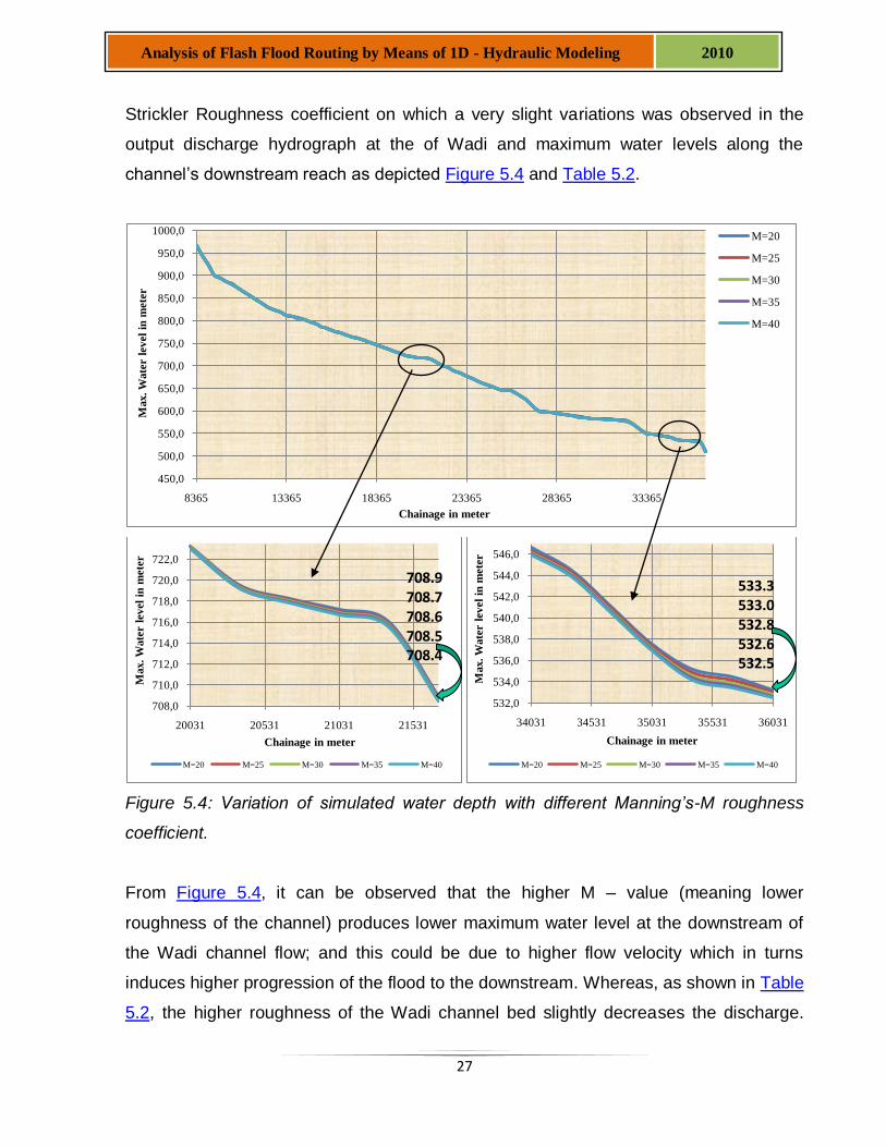
Analysis of Flash Flood Routing by Means of 1D - Hydraulic Modeling 2010
Strickler Roughness coefficient on which a very slight variations was observed in the
output discharge hydrograph at the of Wadi and maximum water levels along the
channel’s downstream reach as depicted Figure 5.4 and Table 5.2.
Figure 5.4: Variation of simulated water depth with different Manning’s-M roughness
coefficient.
From Figure 5.4, it can be observed that the higher M – value (meaning lower
roughness of the channel) produces lower maximum water level at the downstream of
the Wadi channel flow; and this could be due to higher flow velocity which in turns
induces higher progression of the flood to the downstream. Whereas, as shown in Table
5.2, the higher roughness of the Wadi channel bed slightly decreases the discharge.
450,0
500,0
550,0
600,0
650,0
700,0
750,0
800,0
850,0
900,0
950,0
1000,0
8365 13365 18365 23365 28365 33365
Max. W
ate
r l
ev
el
in m
ete
r
Chainage in meter
M=20
M=25
M=30
M=35
M=40
708,0
710,0
712,0
714,0
716,0
718,0
720,0
722,0
20031 20531 21031 21531
Max. W
ate
r l
ev
el
in m
ete
r
Chainage in meter
M=20 M=25 M=30 M=35 M=40
708.9708.7708.6708.5708.4
532,0
534,0
536,0
538,0
540,0
542,0
544,0
546,0
34031 34531 35031 35531 36031
Max. W
ate
r l
ev
el
in m
ete
r
Chainage in meter
M=20 M=25 M=30 M=35 M=40
533.3533.0532.8532.6532.5
28
Analysis of Flash Flood Routing by Means of 1D - Hydraulic Modeling 2010
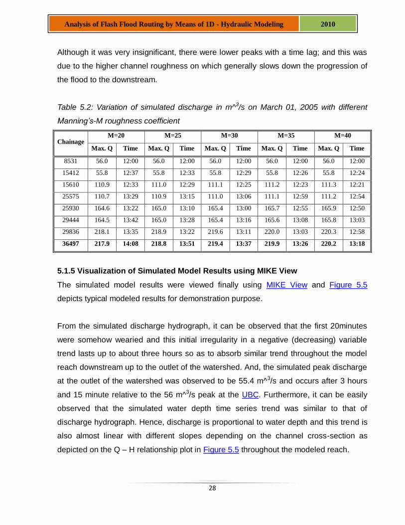
Although it was very insignificant, there were lower peaks with a time lag; and this was
due to the higher channel roughness on which generally slows down the progression of
the flood to the downstream.
Table 5.2: Variation of simulated discharge in m^3/s on March 01, 2005 with different
Manning’s-M roughness coefficient
Chainage M=20 M=25 M=30 M=35 M=40
Max. Q Time Max. Q Time Max. Q Time Max. Q Time Max. Q Time
8531 56.0 12:00 56.0 12:00 56.0 12:00 56.0 12:00 56.0 12:00
15412 55.8 12:37 55.8 12:33 55.8 12:29 55.8 12:26 55.8 12:24
15610 110.9 12:33 111.0 12:29 111.1 12:25 111.2 12:23 111.3 12:21
25575 110.7 13:29 110.9 13:15 111.0 13:06 111.1 12:59 111.2 12:54
25930 164.6 13:22 165.0 13:10 165.4 13:00 165.7 12:55 165.9 12:50
29444 164.5 13:42 165.0 13:28 165.4 13:16 165.6 13:08 165.8 13:03
29836 218.1 13:35 218.9 13:22 219.6 13:11 220.0 13:03 220.3 12:58
36497 217.9 14:08 218.8 13:51 219.4 13:37 219.9 13:26 220.2 13:18
5.1.5 Visualization of Simulated Model Results using MIKE View
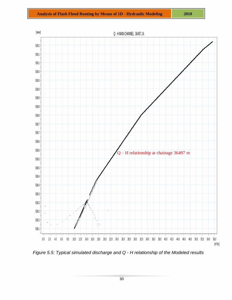
The simulated model results were viewed finally using MIKE View and Figure 5.5
depicts typical modeled results for demonstration purpose.
From the simulated discharge hydrograph, it can be observed that the first 20minutes
were somehow wearied and this initial irregularity in a negative (decreasing) variable
trend lasts up to about three hours so as to absorb similar trend throughout the model
reach downstream up to the outlet of the watershed. And, the simulated peak discharge
at the outlet of the watershed was observed to be 55.4 m^3/s and occurs after 3 hours
and 15 minute relative to the 56 m^3/s peak at the UBC. Furthermore, it can be easily
observed that the simulated water depth time series trend was similar to that of
discharge hydrograph. Hence, discharge is proportional to water depth and this trend is
also almost linear with different slopes depending on the channel cross-section as
depicted on the Q – H relationship plot in Figure 5.5 throughout the modeled reach.

29
Analysis of Flash Flood Routing by Means of 1D - Hydraulic Modeling 2010
00:00:00
1-3-2005
03:00:00 06:00:00 09:00:00 12:00:00 15:00:00 18:00:00 21:00:00 00:00:00
2-3-2005
03:00:00 06:00:00 09:00:00 12:00:00 15:00:00 18:00:00
0.0
5.0
10.0
15.0
20.0
25.0
30.0
35.0
40.0
45.0
50.0
55.0
[m^3/s] Time Series Discharge
Inlet & outlet discharge hydrograph
30
Analysis of Flash Flood Routing by Means of 1D - Hydraulic Modeling 2010
Figure 5.5: Typical simulated discharge and Q - H relationship of the Modeled results
0.0 2.0 4.0 6.0 8.0 10.0 12.0 14.0 16.0 18.0 20.0 22.0 24.0 26.0 28.0 30.0 32.0 34.0 36.0 38.0 40.0 42.0 44.0 46.0 48.0 50.0 52.0 54.0 56.0
[m^3/s]
508.1
508.2
508.2
508.3
508.3
508.4
508.4
508.5
508.5
508.6
508.6
508.7
508.7
508.8
508.8
508.9
508.9
509.0
509.0
509.1
509.1
509.2
[meter] Q - H MAIN CHANNEL 36497.14
Q – H relationship at chainage 36497 m
31
Analysis of Flash Flood Routing by Means of 1D - Hydraulic Modeling 2010
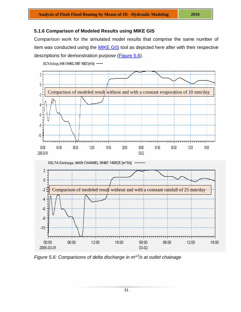
5.1.6 Comparison of Modeled Results using MIKE GIS
Comparison work for the simulated model results that comprise the same number of
item was conducted using the MIKE GIS tool as depicted here after with their respective
descriptions for demonstration purpose (Figure 5.6).
Figure 5.6: Comparisons of delta discharge in m^3/s at outlet chainage
Comparison of modeled result without and with a constant rainfall of 25 mm/day
Comparison of modeled result without and with a constant evaporation of 10 mm/day
32
Analysis of Flash Flood Routing by Means of 1D - Hydraulic Modeling 2010
These above figure shows the comparison analysis of consideration of evaporation and
rainfall rates during model simulation; and it can been concluded that they were not very
significant to consider them during the model set up as they were practically
insignificant bearing in mind the study area.
5.2 Sensitivity Analysis
Sensitivity analysis is a technique used to determine how different values of an
independent variable will impact a particular dependent variable under a given set of
assumptions. Therefore, this study work conducts the sensitivity analysis of the impact
of uncertainties in channel geometry, roughness and impacts of numerical flow
descriptions by creating a given set of scenarios within the study area based on the
prevailing conditions on ground.
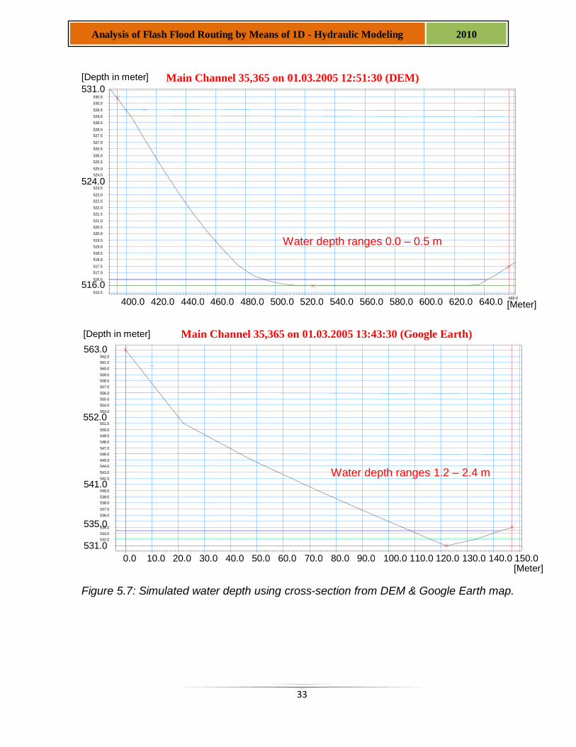
5.2.1 Impacts of uncertainties in channel geometry
It is known that the spatial and temporal variations of rainfall and the concurrent
variation of the abstraction processes such as depressions define the runoff
characteristics resulted from the given rainfall. Thus, when runoff commences, the
geometry of the drainage channels have a large influence on the runoff characteristics
from the watershed; although it was very difficult to quantify the effect. In this study
report, geometry of the channel network of the watershed was analyzed which
comprises basically the shape of cross-section, length, and slope of the channel as
those have a significant impact on the resulted hydrograph within the study area.
Therefore, there was definitely an uncertainty created due to the assumed fixed channel
geometry considered while running the model which might be different with the
prevailing condition as there was difference as well among the DEM and Google Earth
derived model cross-sections as shown on Figure 5.7 as well as annex 1 and 2.
33
Analysis of Flash Flood Routing by Means of 1D - Hydraulic Modeling 2010
Figure 5.7: Simulated water depth using cross-section from DEM & Google Earth map.
0.0 10.0 20.0 30.0 40.0 50.0 60.0 70.0 80.0 90.0 100.0 110.0 120.0 130.0 140.0 150.0 [Meter]
531.0 532.0 533.0 534.0 535.0 536.0 537.0 538.0 539.0 540.0 541.0 542.0 543.0 544.0 545.0 546.0 547.0 548.0 549.0 550.0 551.0 552.0 553.0 554.0 555.0 556.0 557.0 558.0 559.0 560.0 561.0 562.0
563.0
Main Channel 35,365 on 01.03.2005 13:43:30 (Google Earth)
Water depth ranges 1.2 – 2.4 m
[Depth in meter]
400.0 420.0 440.0 460.0 480.0 500.0 520.0 540.0 560.0 580.0 600.0 620.0 640.0 660.0 [Meter]
515.5 516.0
516.5 517.0 517.5 518.0 518.5 519.0 519.5 520.0 520.5 521.0 521.5 522.0 522.5 523.0 523.5 524.0 524.5 525.0 525.5 526.0 526.5 527.0 527.5 528.0 528.5 529.0 529.5 530.0 530.5
531.0
[Depth in meter] Main Channel 35,365 on 01.03.2005 12:51:30 (DEM)
Water depth ranges 0.0 – 0.5 m
34
Analysis of Flash Flood Routing by Means of 1D - Hydraulic Modeling 2010
As shown on Figure 5.7, it can be concluded that there exist a very significant impact on
the simulated minimum and maximum water depth time series throughout the model
reach due to the uncertainty of the accuracy of the utilized cross-section inputs.
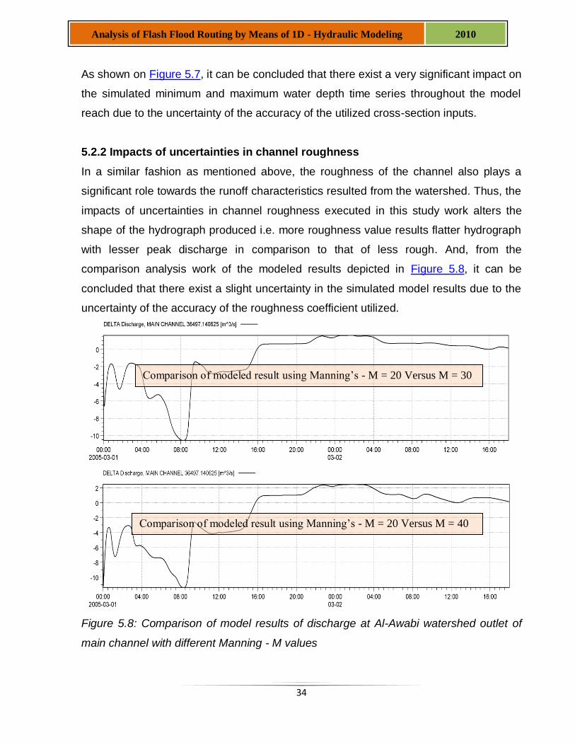
5.2.2 Impacts of uncertainties in channel roughness
In a similar fashion as mentioned above, the roughness of the channel also plays a
significant role towards the runoff characteristics resulted from the watershed. Thus, the
impacts of uncertainties in channel roughness executed in this study work alters the
shape of the hydrograph produced i.e. more roughness value results flatter hydrograph
with lesser peak discharge in comparison to that of less rough. And, from the
comparison analysis work of the modeled results depicted in Figure 5.8, it can be
concluded that there exist a slight uncertainty in the simulated model results due to the
uncertainty of the accuracy of the roughness coefficient utilized.
Figure 5.8: Comparison of model results of discharge at Al-Awabi watershed outlet of
main channel with different Manning - M values
Comparison of modeled result using Manning’s - M = 20 Versus M = 40
Comparison of modeled result using Manning’s - M = 20 Versus M = 30
35
Analysis of Flash Flood Routing by Means of 1D - Hydraulic Modeling 2010
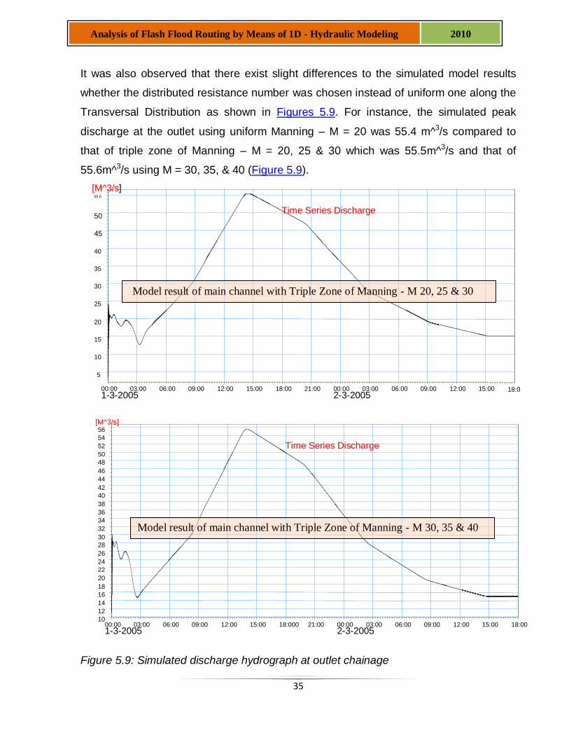
It was also observed that there exist slight differences to the simulated model results
whether the distributed resistance number was chosen instead of uniform one along the
Transversal Distribution as shown in Figures 5.9. For instance, the simulated peak
discharge at the outlet using uniform Manning – M = 20 was 55.4 m^3/s compared to
that of triple zone of Manning – M = 20, 25 & 30 which was 55.5m^3/s and that of
55.6m^3/s using M = 30, 35, & 40 (Figure 5.9).
Figure 5.9: Simulated discharge hydrograph at outlet chainage
00:00 1-3-2005
03:00 06:00 09:00 12:00 15:00 18:000 21:00 00:00 2-3-2005
03:00 06:00 09:00 12:00 15:00 18:00 10 12
14
16 18
20
22 24
26
28 30
32
34 36
38
40 42
44
46
48 50
52
54 56
[M^3/s]
Time Series Discharge
Model result of main channel with Triple Zone of Manning - M 30, 35 & 40
00:00 1-3-2005
03:00 06:00 09:00 12:00 15:00 18:00 21:00 00:00 2-3-2005
03:00 06:00 09:00 12:00 15:00 18:0
5
10
15
20
25
30
35
40
45
50
55.0 [M^3/s]
Time Series Discharge
Model result of main channel with Triple Zone of Manning - M 20, 25 & 30
36
Analysis of Flash Flood Routing by Means of 1D - Hydraulic Modeling 2010
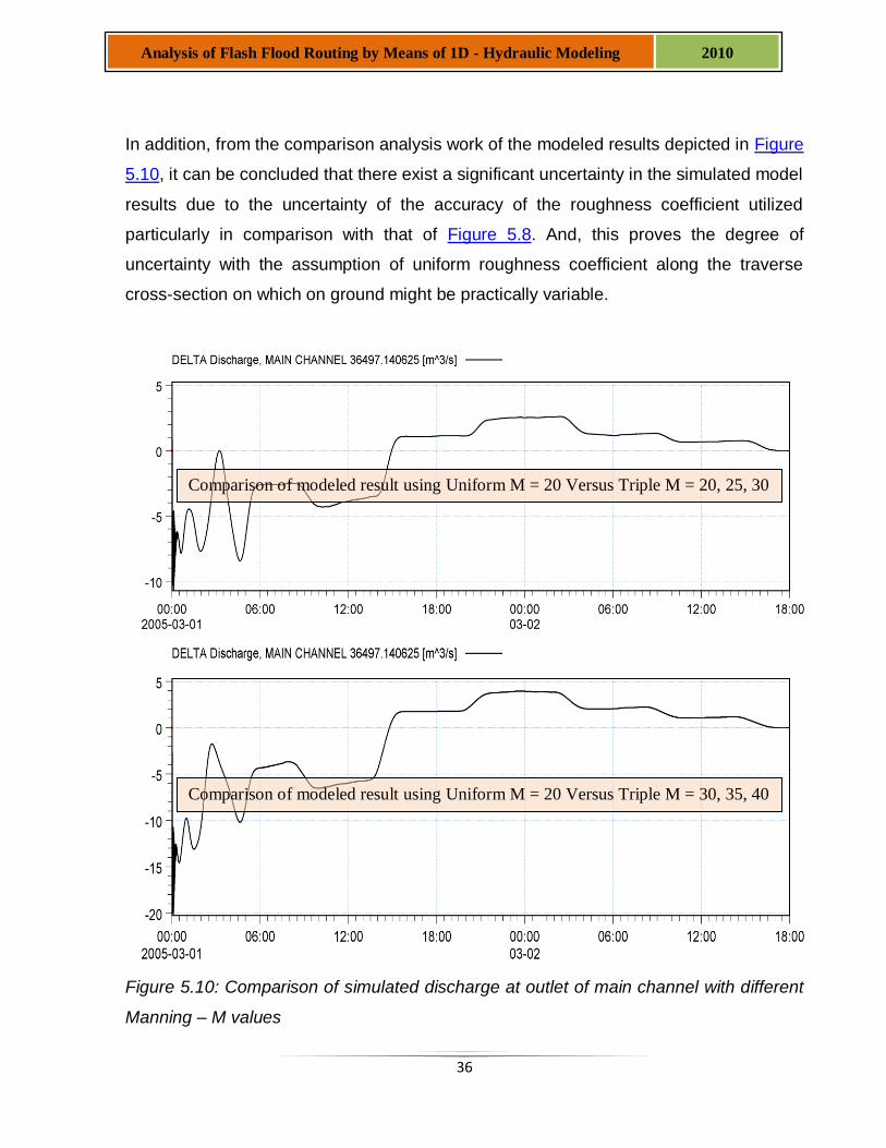
In addition, from the comparison analysis work of the modeled results depicted in Figure
5.10, it can be concluded that there exist a significant uncertainty in the simulated model
results due to the uncertainty of the accuracy of the roughness coefficient utilized
particularly in comparison with that of Figure 5.8. And, this proves the degree of
uncertainty with the assumption of uniform roughness coefficient along the traverse
cross-section on which on ground might be practically variable.
Figure 5.10: Comparison of simulated discharge at outlet of main channel with different
Manning – M values
Comparison of modeled result using Uniform M = 20 Versus Triple M = 30, 35, 40
Comparison of modeled result using Uniform M = 20 Versus Triple M = 20, 25, 30
37
Analysis of Flash Flood Routing by Means of 1D - Hydraulic Modeling 2010
Therefore, from all reputed figures above in this section, it can be concluded that the
higher channel roughness coefficient of the Wadi bed decreases the resulted runoff at
the downstream of Al-Awabi Wadi; and of course due to the certain degree of
uncertainty level on the estimated roughness coefficient utilized a minor variations was
observed in the modeled results in all the model runs executed.
5.2.3 Impacts of numerical flow descriptions
The numerical flow descriptions are derived through the continuity equation in one
dimensional form and a simplified form of the momentum equation. Thus, there is
definitely an impact as the type of flow found in the prevailing natural watershed was not
absolutely the same with the model set up. For instance, it was realized that there exist
a significant difference with the simulated results obtained using the fully dynamic option
(Figure 5.11) versus the diffusive wave option (Figure 5.12) on which it was noticed a
huge error occurred at early time of simulation at the upstream of the model reach in the
second case.
Figure 5.13 compares the simulated results using the different options of wave
approximation provided at the HD parameter MIKE module. And from this comparison
figure, it can be easily observed that there exist a slight difference to the model results
as to which flow condition option was taken and the uncertainty level at deciding the
correct flow conditions during model simulation. For instance, it was noticed that the
kinematic wave option was producing an incomplete simulation; and this could be
because the kinematic wave has certain degree of uncertainty to that of the real one on
ground due to transmission losses, for instance, which leads to no hydrologic balance
between the rainfall events.
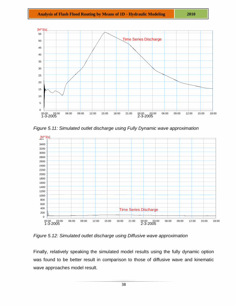
38
Analysis of Flash Flood Routing by Means of 1D - Hydraulic Modeling 2010
Figure 5.11: Simulated outlet discharge using Fully Dynamic wave approximation
Figure 5.12: Simulated outlet discharge using Diffusive wave approximation
Finally, relatively speaking the simulated model results using the fully dynamic option
was found to be better result in comparison to those of diffusive wave and kinematic
wave approaches model result.
00:00 1-3-2005
03:00 06:00 09:00 12:00 15:00 18:00 21:00 00:00 2-3-2005
03:00 06:00 09:00 12:00 15:00 18:00
0
200
400
600
800
1000
1200
1400
1600
1800
2000
2200
2400
2600
2800
3000
3200
3400
3600.0 [M^3/s]
Time Series Discharge
00:00 1-3-2005
03:00 06:00 09:00 12:00 15:00 18:00 21:00 00:00 2-3-2005
03:00 06:00 09:00 12:00 15:00 18:00
0
5
10
15
20
25
30
35
40
45
50
55
[M^3/s]
Time Series Discharge
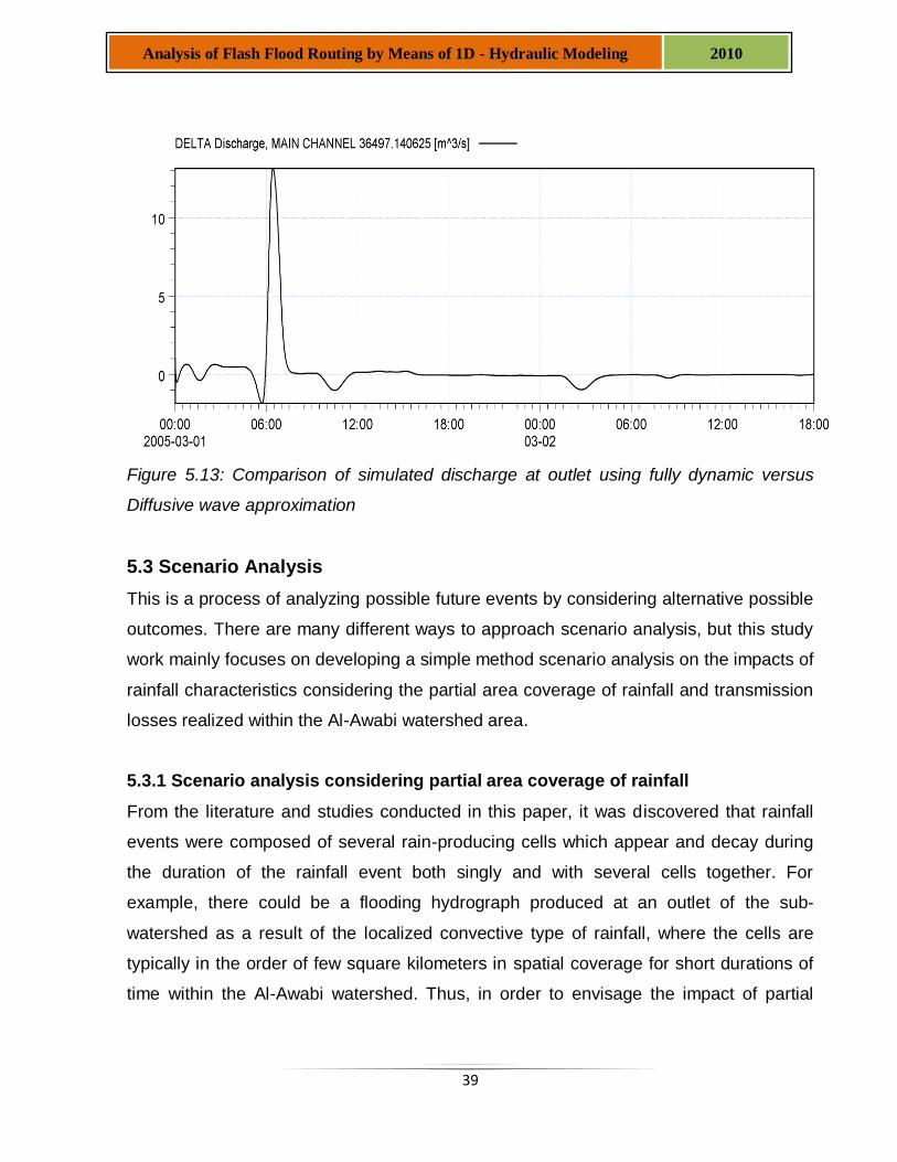
39
Analysis of Flash Flood Routing by Means of 1D - Hydraulic Modeling 2010
Figure 5.13: Comparison of simulated discharge at outlet using fully dynamic versus
Diffusive wave approximation
5.3 Scenario Analysis
This is a process of analyzing possible future events by considering alternative possible
outcomes. There are many different ways to approach scenario analysis, but this study
work mainly focuses on developing a simple method scenario analysis on the impacts of
rainfall characteristics considering the partial area coverage of rainfall and transmission
losses realized within the Al-Awabi watershed area.
5.3.1 Scenario analysis considering partial area coverage of rainfall
From the literature and studies conducted in this paper, it was discovered that rainfall
events were composed of several rain-producing cells which appear and decay during
the duration of the rainfall event both singly and with several cells together. For
example, there could be a flooding hydrograph produced at an outlet of the sub-
watershed as a result of the localized convective type of rainfall, where the cells are
typically in the order of few square kilometers in spatial coverage for short durations of
time within the Al-Awabi watershed. Thus, in order to envisage the impact of partial
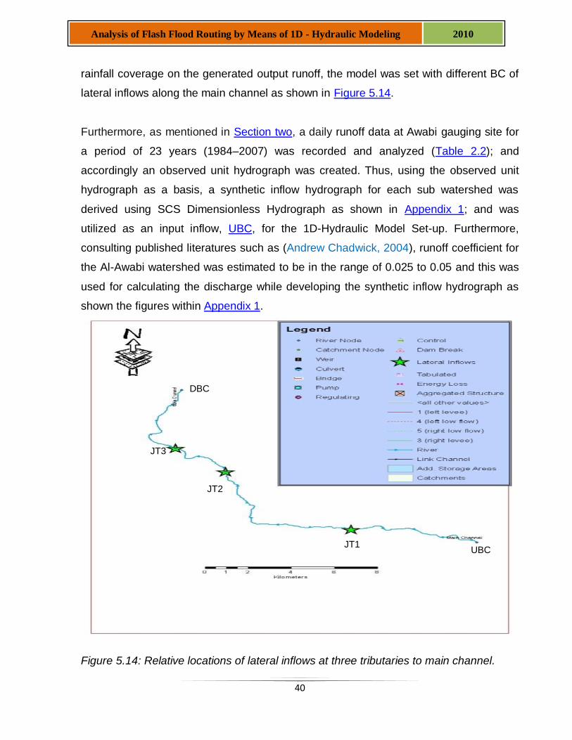
40
Analysis of Flash Flood Routing by Means of 1D - Hydraulic Modeling 2010
rainfall coverage on the generated output runoff, the model was set with different BC of
lateral inflows along the main channel as shown in Figure 5.14.
Furthermore, as mentioned in Section two, a daily runoff data at Awabi gauging site for
a period of 23 years (1984–2007) was recorded and analyzed (Table 2.2); and
accordingly an observed unit hydrograph was created. Thus, using the observed unit
hydrograph as a basis, a synthetic inflow hydrograph for each sub watershed was
derived using SCS Dimensionless Hydrograph as shown in Appendix 1; and was
utilized as an input inflow, UBC, for the 1D-Hydraulic Model Set-up. Furthermore,
consulting published literatures such as (Andrew Chadwick, 2004), runoff coefficient for
the Al-Awabi watershed was estimated to be in the range of 0.025 to 0.05 and this was
used for calculating the discharge while developing the synthetic inflow hydrograph as
shown the figures within Appendix 1.
Figure 5.14: Relative locations of lateral inflows at three tributaries to main channel.
JT1
JT2
JT3
UBC
DBC
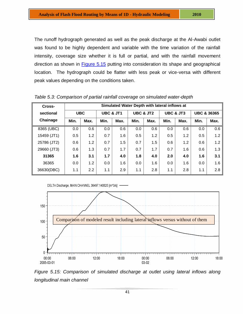
41
Analysis of Flash Flood Routing by Means of 1D - Hydraulic Modeling 2010
The runoff hydrograph generated as well as the peak discharge at the Al-Awabi outlet
was found to be highly dependent and variable with the time variation of the rainfall
intensity, coverage size whether it is full or partial, and with the rainfall movement
direction as shown in Figure 5.15 putting into consideration its shape and geographical
location. The hydrograph could be flatter with less peak or vice-versa with different
peak values depending on the conditions taken.
Table 5.3: Comparison of partial rainfall coverage on simulated water-depth
Cross-
sectional
Chainage
Simulated Water Depth with lateral inflows at
UBC UBC & JT1 UBC & JT2 UBC & JT3 UBC & 36365
Min. Max. Min. Max. Min. Max. Min. Max. Min. Max.
8365 (UBC) 0.0 0.6 0.0 0.6 0.0 0.6 0.0 0.6 0.0 0.6
15459 (JT1) 0.5 1.2 0.7 1.6 0.5 1.2 0.5 1.2 0.5 1.2
25786 (JT2) 0.6 1.2 0.7 1.5 0.7 1.5 0.6 1.2 0.6 1.2
29660 (JT3) 0.6 1.3 0.7 1.7 0.7 1.7 0.7 1.6 0.6 1.3
31365 1.6 3.1 1.7 4.0 1.8 4.0 2.0 4.0 1.6 3.1
36365 0.0 1.2 0.0 1.6 0.0 1.6 0.0 1.6 0.0 1.6
36630(DBC) 1.1 2.2 1.1 2.9 1.1 2.8 1.1 2.8 1.1 2.8
Figure 5.15: Comparison of simulated discharge at outlet using lateral inflows along
longitudinal main channel
Comparison of modeled result including lateral inflows versus without of them
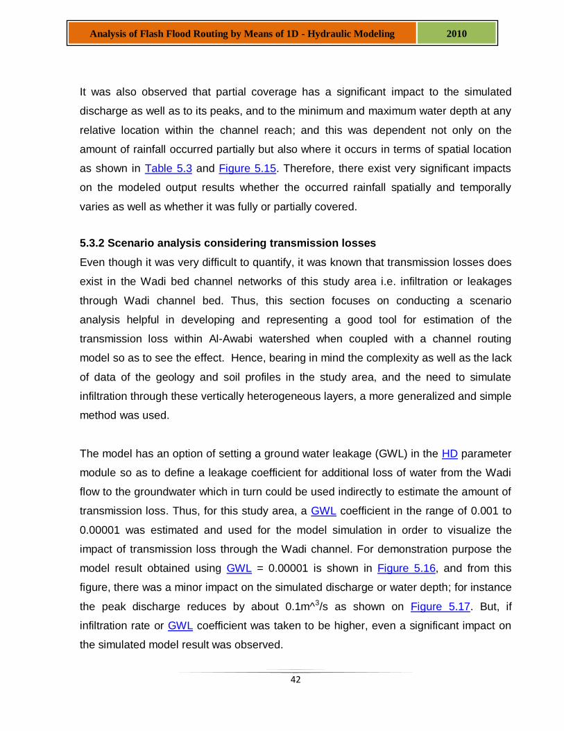
42
Analysis of Flash Flood Routing by Means of 1D - Hydraulic Modeling 2010
It was also observed that partial coverage has a significant impact to the simulated
discharge as well as to its peaks, and to the minimum and maximum water depth at any
relative location within the channel reach; and this was dependent not only on the
amount of rainfall occurred partially but also where it occurs in terms of spatial location
as shown in Table 5.3 and Figure 5.15. Therefore, there exist very significant impacts
on the modeled output results whether the occurred rainfall spatially and temporally
varies as well as whether it was fully or partially covered.
5.3.2 Scenario analysis considering transmission losses
Even though it was very difficult to quantify, it was known that transmission losses does
exist in the Wadi bed channel networks of this study area i.e. infiltration or leakages
through Wadi channel bed. Thus, this section focuses on conducting a scenario
analysis helpful in developing and representing a good tool for estimation of the
transmission loss within Al-Awabi watershed when coupled with a channel routing
model so as to see the effect. Hence, bearing in mind the complexity as well as the lack
of data of the geology and soil profiles in the study area, and the need to simulate
infiltration through these vertically heterogeneous layers, a more generalized and simple
method was used.
The model has an option of setting a ground water leakage (GWL) in the HD parameter
module so as to define a leakage coefficient for additional loss of water from the Wadi
flow to the groundwater which in turn could be used indirectly to estimate the amount of
transmission loss. Thus, for this study area, a GWL coefficient in the range of 0.001 to
0.00001 was estimated and used for the model simulation in order to visualize the
impact of transmission loss through the Wadi channel. For demonstration purpose the
model result obtained using GWL = 0.00001 is shown in Figure 5.16, and from this
figure, there was a minor impact on the simulated discharge or water depth; for instance
the peak discharge reduces by about 0.1m^3/s as shown on Figure 5.17. But, if
infiltration rate or GWL coefficient was taken to be higher, even a significant impact on
the simulated model result was observed.
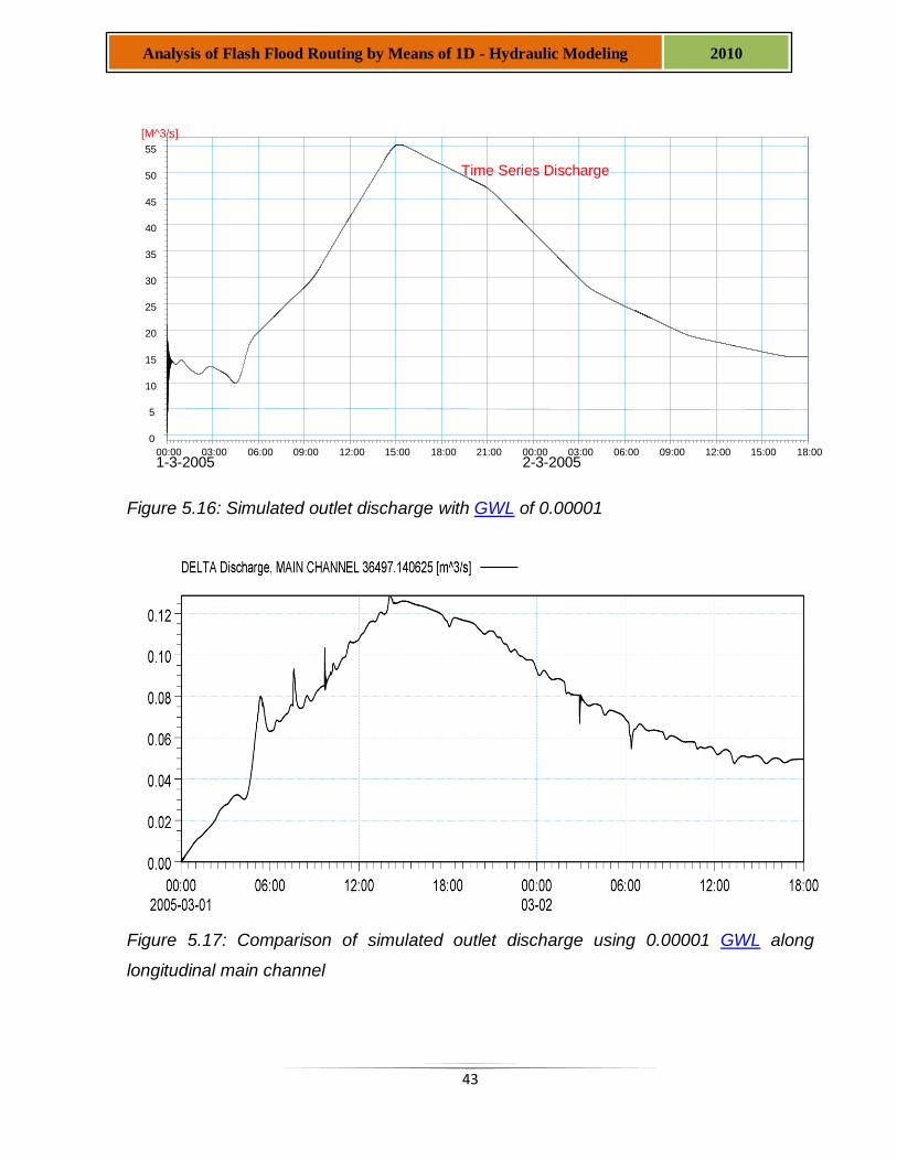
43
Analysis of Flash Flood Routing by Means of 1D - Hydraulic Modeling 2010
Figure 5.16: Simulated outlet discharge with GWL of 0.00001
Figure 5.17: Comparison of simulated outlet discharge using 0.00001 GWL along
longitudinal main channel
00:00 1-3-2005
03:00 06:00 09:00 12:00 15:00 18:00 21:00 00:00 2-3-2005
03:00 06:00 09:00 12:00 15:00 18:00
0
5
10
15
20
25
30
35
40
45
50
55
[M^3/s]
Time Series Discharge
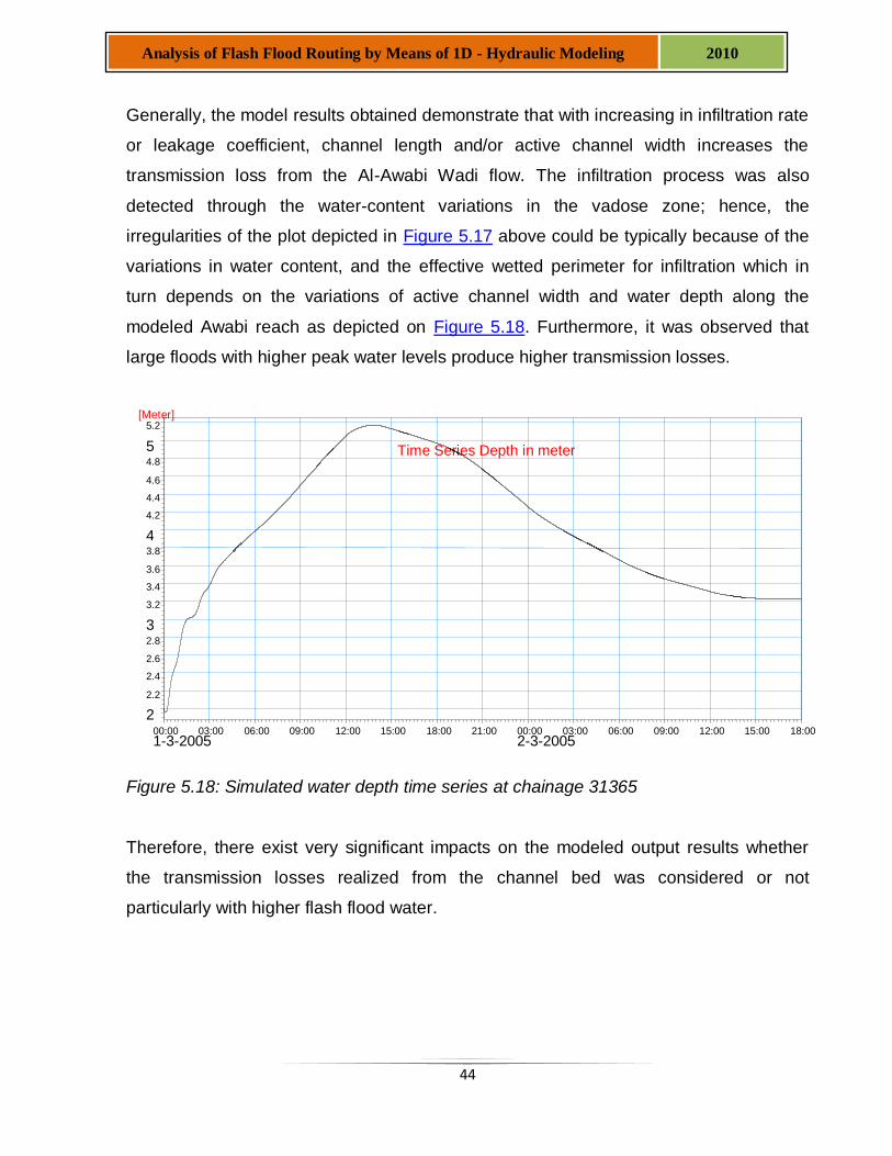
44
Analysis of Flash Flood Routing by Means of 1D - Hydraulic Modeling 2010
Generally, the model results obtained demonstrate that with increasing in infiltration rate
or leakage coefficient, channel length and/or active channel width increases the
transmission loss from the Al-Awabi Wadi flow. The infiltration process was also
detected through the water-content variations in the vadose zone; hence, the
irregularities of the plot depicted in Figure 5.17 above could be typically because of the
variations in water content, and the effective wetted perimeter for infiltration which in
turn depends on the variations of active channel width and water depth along the
modeled Awabi reach as depicted on Figure 5.18. Furthermore, it was observed that
large floods with higher peak water levels produce higher transmission losses.
Figure 5.18: Simulated water depth time series at chainage 31365
Therefore, there exist very significant impacts on the modeled output results whether
the transmission losses realized from the channel bed was considered or not
particularly with higher flash flood water.
00:00 1-3-2005
03:00 06:00 09:00 12:00 15:00 18:00 21:00 00:00 2-3-2005
03:00 06:00 09:00 12:00 15:00 18:00
2
2.2
2.4
2.6
2.8
3
3.2
3.4
3.6
3.8
4
4.2
4.4
4.6
4.8
5
5.2 [Meter]
Time Series Depth in meter
45
Analysis of Flash Flood Routing by Means of 1D - Hydraulic Modeling 2010
6. Conclusion
Analysis of flash flood routing within the Al-Awabi watershed channels were investigated
in this study, focusing on: (1) Preparation of inflow hydrographs and estimation of model
inflows BC; (2) flood routing model set up, (3) sensitivity analysis work on certain
uncertainties such as channel geometry and roughness, and (4) studying the scenario
analysis on impacts of rainfall characteristics and transmission loss. And, the main
conclusions inferred from the study are:
As it had been already reputed above, there was scarcity of data which was
relevant for the model setup; hence an estimated inflow hydrographs was applied
during the model simulation by utilizing the recorded runoff data at Awabi
gauging as a basis. Thus, it was very difficult to talk about quality of data, and it
was also not easy task to model and forecast inflow hydrographs bearing in mind
the lack of enough available data in the target area, Al-Awabi watershed.
Furthermore, Channel cross-sections were one of the main inputs to the 1D-
Hydraulic Model used for the analysis of flash flood routing of the Al-Awabi
watershed and it was observed that there were huge uncertainties with the
values utilized for the model run which contributes to poor model data quality.
The performance of the calibrated 1D-Hydraulic Model i.e. MIKE 11 HD was
assessed and validated to simulate the flash flood routing analysis at different
cross-sections of the main channel reach. And from this study, although there
were major gap and problems in data as well as in the prevailing topography,
slope and other HD parameters, it was concluded that the 1D-Hydraulic
Modelling utilized for flood routing analysis work can be applied for the Al-Awabi
watershed. Hence, the calibrated model can be used to simulate possible future
floods.
From the simulated model results, it was observed that the model was sensitive
to the type BC chosen and taken, channel cross sections and its roughness
46
Analysis of Flash Flood Routing by Means of 1D - Hydraulic Modeling 2010
coefficient utilized throughout the model reach. Furthermore, this study work
conducts the sensitivity analysis of the impact of uncertainties in channel
geometry, roughness and impacts of numerical flow descriptions; and all cases it
was observed that there was a little impact on the simulated model results as the
result of the reputed uncertainty as discussed earlier. Hence, it can be concluded
that the model was not robust.
Although further insight work is required in order to come up with a concrete
conclusion about its impact quantification due to partial rainfall coverage and
transmission losses via the Wade channel beds, it was noticed that there exist an
impact to the simulated downstream discharge of the study area.
47
Analysis of Flash Flood Routing by Means of 1D - Hydraulic Modeling 2010
7. Limitation of study and Recommendation
As it had been mentioned in the previous sections respectively, the main limitation and
drawback of this study work was lack and/or scarcity of data requirement as everything
was almost an estimate which makes the whole task executed and covered in this
thesis like a virtual work. For instance, the BC used were quite questionable for their
practicability as well as there was certain degree of uncertainty with the cross sections,
and the model parameters such as the Manning’s roughness coefficient used in model
setup.
Having said that here are some recommendations drawn out of this study work and
reputed below:
The use of modern surveying technologies such as Total Station survey
measurements are recommended as they could provide better results with higher
degree of accuracy about the topography of the study area than the utilized DEM
and Google Earth map information. And this could be practically executed in this
study area by taking field survey measurements for the whole Al-Awabi
watershed topography with special emphasis on and along the wade channel
networks. Therefore, it would be advisable to make a pre-model test for a smaller
sub-watershed with the entire data requirement full-filled on one of the tributary
channels rather than analyzing for the whole Al-Awabi watershed. As the HD
model requires continuous flow of water with adequate channel geometry
information; but, to the contrary, the prevailing condition in this study area is
Ephemeral River i.e. wades which has no flow of water in most of the time period
as well as the topography is really ragged and steep slope area.
In order to have better understanding about the dynamics of the flash flood that
could occur within the watershed, an adequate number of structures/stations
have to be set up along the main channel such as weirs, culverts, and control
structures. For example, there could be a flooding hydrograph produced at an
48
Analysis of Flash Flood Routing by Means of 1D - Hydraulic Modeling 2010
outlet of the sub-watershed as a result of the localized convective type of rainfall
for short durations of time within the Al-Awabi watershed.
Last but not least, further investigation work is recommended which embraces,
for example, comparison of the same tasks that could be obtained from the rest
of watersheds found at the mountainous part of the Batinah region, Oman; so as
to have a better understanding of the flood routing analysis work which couples
the hydrological water balance effect between the rainfall events. Therefore, this
paper can be used as a starting material for further detailed modeling work that
encompasses the whole channel network of the entire watershed area.
49
Analysis of Flash Flood Routing by Means of 1D - Hydraulic Modeling 2010
Theses
1. This study was conducted at the mountainous catchment part of Batinah Region
of the Sultanate of Oman called Al-Awabi watershed which is about 260km2 in
area and with about 40 Km long main channel.
2. It was observed that, the drainage pattern of Al-Awabi watershed can be
categorized as Dendritic pattern where tributary branch and erode headwater in
random fashion which results in slopes with no predominant direction or
orientation; as well as Rectangular pattern mainly occurring in this case along
and near to the main channel network as shown in Figure 2.7.
3. Because the Al-Awabi channel network comprises a Wadi main channel which
stretches for about 40 Km with its bed level ranging from about 500m at the
downstream end to 2200m at the upstream end a.m.s.l, and a numerous number
of channel braches on top of the uncertainty on channel geometry; it was
practically difficult task to set up a model for the whole watershed. Therefore, the
model set up was executed only for the lower about 24 Km long of the main
channel.
4. There was scarcity of rainfall – runoff data which was relevant for the model
setup; hence an estimated inflow hydrographs was applied during the model
simulation by utilizing the recorded runoff data at Awabi gauge as a basis.
5. Channel cross-sections were the main input to the 1D-Hydraulic Model used for
the analysis of flash flood routing of the Al-Awabi watershed. Hence, a
methodology for extracting the channel cross-sections from ASTER DEM
(27mX27m) and Google Earth map were used in this study area.
6. From this study, although there were major gap and problems in data as well as
in the prevailing topography, slope and other HD parameters, it was concluded
that the 1D-Hydraulic Modelling utilized for flood routing analysis work can be
applied for the Al-Awabi watershed.
7. From the simulated model results, it was observed that the calibrated model was
sensitive to the type BC chosen and taken, channel cross sections and its
roughness coefficient utilized throughout the model reach.
50
Analysis of Flash Flood Routing by Means of 1D - Hydraulic Modeling 2010
8. Although further insight work is required in order to come up with a concrete
conclusion about its impact quantification due to partial rainfall coverage and
transmission losses via the Wade channel beds, it was noticed that there exist an
impact to the simulated downstream discharge within the study area.
9. The main limitation and drawback of this study work was lack and/or scarcity of
model data requirement as everything was almost an estimate which makes the
whole task executed and covered in this thesis like a virtual work.
10. Finally, this paper can be used as a starting material for further detailed modeling
work that encompasses the whole channel network of the entire watershed area
so as to have a better understanding of the flood routing analysis work.
51
Analysis of Flash Flood Routing by Means of 1D - Hydraulic Modeling 2010
Bibliography
Andrew Chadwick, J. M. (2004). HYDRAULICS IN CIVIL AND ENVIRONMENTAL
ENGINEERING (Fourth ed.). London, EC4P 4EE, UK: Spon Press.
Brutsaert, W. (2005). Hydrology An Introduction (2006 ed.). Cambridge, UK: Cambridge
University Press.
DHI. (2009). MIKE 11 - A Modelling System for Rivers and Channels. Denmark: DHI.
Garbrecht, L. W. (2000). The Treatment of Flat Areas and Depressions in Automated
Drainage Analysis for Raster Digital Elevation Models. In A. G. Montgomery,
Hydrological Applications of GIS (pp. 23-35). Chichester, West Sussex PO19 1UD,
England: John Wiley & Sons Ltd.
GDEM, A. (2009, June 29). ASTER GDEM. Retrieved March 31, 2010, from ASTER
GDEM: http://www.gdem.aster.ersdac.or.jp/
John A. Roberson, J. J. (1988). Hydraulic Engineering (1988 ed.). Boston,
Massachusetts 02108, USA: Houghton Mifflin Company.
Mays, L. W. (2005). WATER RESOURCES ENGINEERING (2005 ed.). Tempe,
Arizona, USA: Wiley & Sons.
Shamsi, U. (2005). GIS Applications for Water, Wastewater, and Stormwater Systems.
Boca Raton, Florida 33431, USA: CRC Press.
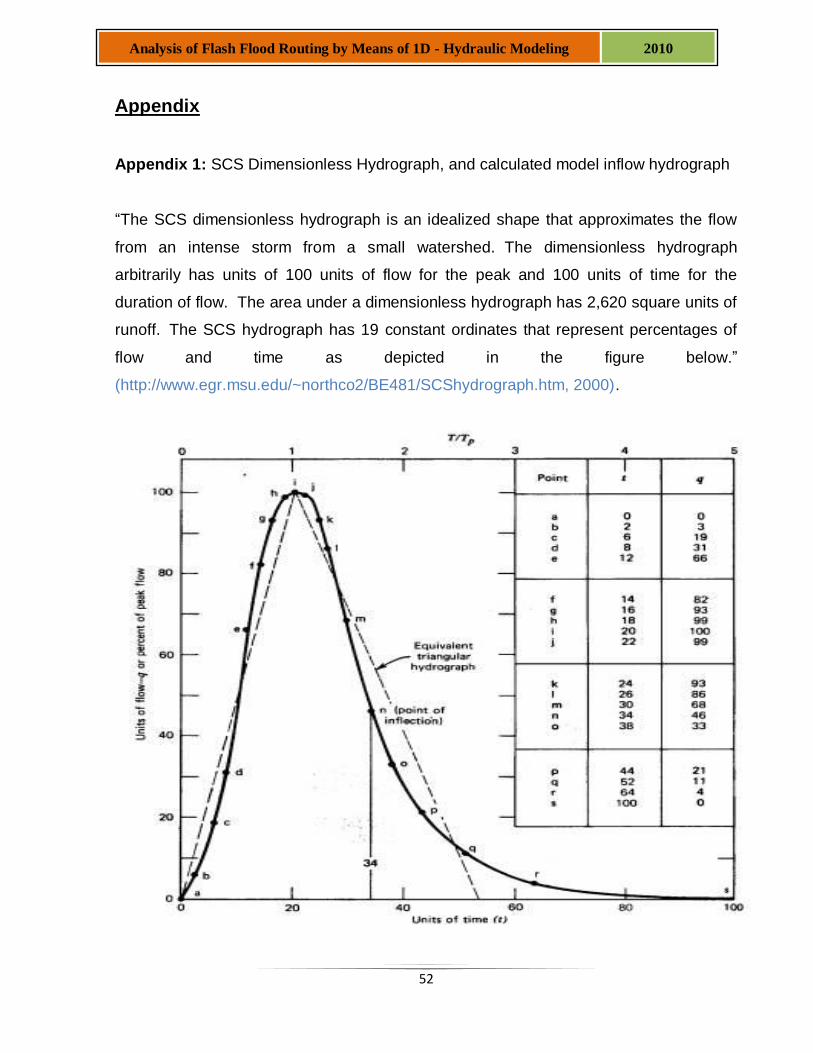
52
Analysis of Flash Flood Routing by Means of 1D - Hydraulic Modeling 2010
Appendix
Appendix 1: SCS Dimensionless Hydrograph, and calculated model inflow hydrograph
“The SCS dimensionless hydrograph is an idealized shape that approximates the flow
from an intense storm from a small watershed. The dimensionless hydrograph
arbitrarily has units of 100 units of flow for the peak and 100 units of time for the
duration of flow. The area under a dimensionless hydrograph has 2,620 square units of
runoff. The SCS hydrograph has 19 constant ordinates that represent percentages of
flow and time as depicted in the figure below.”
(http://www.egr.msu.edu/~northco2/BE481/SCShydrograph.htm, 2000).
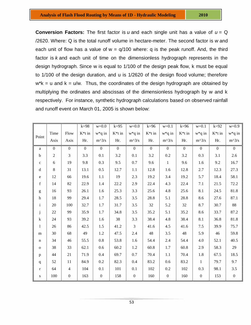
53
Analysis of Flash Flood Routing by Means of 1D - Hydraulic Modeling 2010
Conversion Factors: The first factor is u and each single unit has a value of u = Q
/2620. Where: Q is the total runoff volume in hectare-meter. The second factor is w and
each unit of flow has a value of w = q/100 where: q is the peak runoff. And, the third
factor is k and each unit of time on the dimensionless hydrograph represents in the
design hydrograph. Since w is equal to 1/100 of the design peak flow, k must be equal
to 1/100 of the design duration, and u is 1/2620 of the design flood volume; therefore
w*k = u and k = u/w. Thus, the coordinates of the design hydrograph are obtained by
multiplying the ordinates and abscissas of the dimensionless hydrograph by w and k
respectively. For instance, synthetic hydrograph calculations based on observed rainfall
and runoff event on March 01, 2005 is shown below:
k=98 w=0.0 k=95 w=0.0 k=96 w=0.1 k=96 w=0.1 k=92 w=0.9
Point Time
Axis
Flow
Axis
K*t in
Hr.
w*q in
m^3/s
K*t in
Hr.
w*q in
m^3/s
K*t in
Hr.
w*q in
m^3/s
K*t in
Hr.
w*q in
m^3/s
K*t in
Hr.
w*q in
m^3/s
a 0 0 0 0 0 0 0 0 0 0 0 0
b 2 3 3.3 0.1 3.2 0.1 3.2 0.2 3.2 0.3 3.1 2.6
c 6 19 9.8 0.3 9.5 0.7 9.6 1 9.6 1.6 9.2 16.7
d 8 31 13.1 0.5 12.7 1.1 12.8 1.6 12.8 2.7 12.3 27.3
e 12 66 19.6 1.1 19 2.3 19.2 3.4 19.2 5.7 18.4 58.1
f 14 82 22.9 1.4 22.2 2.9 22.4 4.3 22.4 7.1 21.5 72.2
g 16 93 26.1 1.6 25.3 3.3 25.6 4.8 25.6 8.1 24.5 81.8
h 18 99 29.4 1.7 28.5 3.5 28.8 5.1 28.8 8.6 27.6 87.1
i 20 100 32.7 1.7 31.7 3.5 32 5.2 32 8.7 30.7 88
j 22 99 35.9 1.7 34.8 3.5 35.2 5.1 35.2 8.6 33.7 87.2
k 24 93 39.2 1.6 38 3.3 38.4 4.8 38.4 8.1 36.8 81.8
l 26 86 42.5 1.5 41.2 3 41.6 4.5 41.6 7.5 39.9 75.7
m 30 68 49 1.2 47.5 2.4 48 3.5 48 5.9 46 59.8
n 34 46 55.5 0.8 53.8 1.6 54.4 2.4 54.4 4.0 52.1 40.5
o 38 33 62.1 0.6 60.2 1.2 60.8 1.7 60.8 2.9 58.3 29
p 44 21 71.9 0.4 69.7 0.7 70.4 1.1 70.4 1.8 67.5 18.5
q 52 11 84.9 0.2 82.3 0.4 83.2 0.6 83.2 1 79.7 9.7
r 64 4 104 0.1 101 0.1 102 0.2 102 0.3 98.1 3.5
s 100 0 163 0 158 0 160 0 160 0 153 0
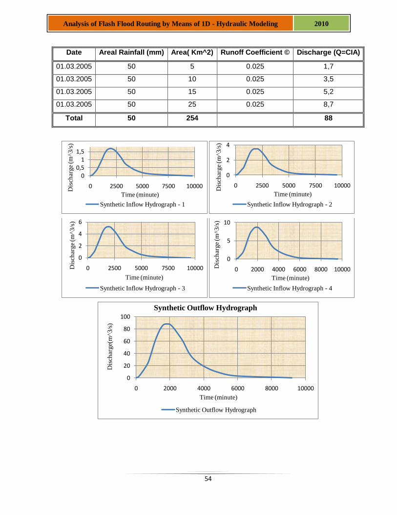
54
Analysis of Flash Flood Routing by Means of 1D - Hydraulic Modeling 2010
Date Areal Rainfall (mm) Area( Km^2) Runoff Coefficient © Discharge (Q=CIA)
01.03.2005 50 5 0.025 1,7
01.03.2005 50 10 0.025 3,5
01.03.2005 50 15 0.025 5,2
01.03.2005 50 25 0.025 8,7
Total 50 254 88
00,5
11,5
0 2500 5000 7500 10000
Dis
char
ge
(m^3/s
)
Time (minute)
Synthetic Inflow Hydrograph - 1
0
2
4
0 2500 5000 7500 10000
Dis
char
ge
(m^3/s
)
Time (minute)
Synthetic Inflow Hydrograph - 2
0
2
4
6
0 2500 5000 7500 10000Dis
char
ge
(m^3
/s)
Time (minute)
Synthetic Inflow Hydrograph - 3
0
5
10
0 2000 4000 6000 8000 10000Dis
char
ge
(m^3
/s)
Time (minute)
Synthetic Inflow Hydrograph - 4
0
20
40
60
80
100
0 2000 4000 6000 8000 10000
Dis
char
ge(
m^3
/s)
Time (minute)
Synthetic Outflow Hydrograph
Synthetic Outflow Hydrograph
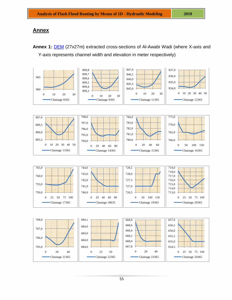
55
Analysis of Flash Flood Routing by Means of 1D - Hydraulic Modeling 2010
Annex
Annex 1: DEM (27x27m) extracted cross-sections of Al-Awabi Wadi (where X-axis and
Y-axis represents channel width and elevation in meter respectively)
960
965
0 10 20 30
Chainage 8365
899,3
899,4
899,5
899,6
899,7
899,8
0 10 20 30
Chainage 9365
845,0
845,5
846,0
846,5
847,0
0 10 20 30
Chainage 11365
834,0
835,0
836,0
837,0
0 10 20 30 40 50
Chainage 12365
805,5
806,0
806,5
807,0
0 10 20 30 40 50
Chainage 13365
794,0
795,0
796,0
797,0
798,0
0 20 40 60 80
Chainage 14365
780,0
781,0
782,0
783,0
784,0
0 20 40 60
Chainage 15365
760,0
765,0
770,0
775,0
0 50 100 150
Chainage 16365
750,0
755,0
760,0
765,0
0 25 50 75 100
Chainage 17365
740,0
741,0
742,0
743,0
744,0
0 20 40 60 80
Chainage 18635
726,5
727,0
727,5
728,0
728,5
0 50 100 150
Chainage 19365
713,0
714,0
715,0
716,0
717,0
718,0
719,0
0 25 50 75 100
Chainage 20365
705,0
706,0
707,0
708,0
0 20 40
Chainage 21365
684,0
684,0
684,0
684,0
684,1
0 25 50
Chainage 22365
667,8
668,0
668,2
668,4
668,6
668,8
0 20 40
Chainage 23365
654,5
655,0
655,5
656,0
656,5
657,0
0 25 50 75 100
Chainage 24365
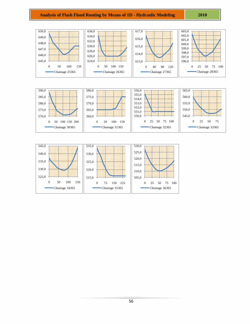
56
Analysis of Flash Flood Routing by Means of 1D - Hydraulic Modeling 2010
645,0
646,0
647,0
648,0
649,0
650,0
0 50 100 150
Chainage 25365
624,0
626,0
628,0
630,0
632,0
634,0
636,0
0 50 100 150
Chainage 26365
613,0
614,0
615,0
616,0
617,0
0 40 80 120
Chainage 27365
596,0
597,0
598,0
599,0
600,0
601,0
602,0
603,0
0 25 50 75 100
Chainage 28365
570,0
575,0
580,0
585,0
590,0
0 50 100 150 200
Chainage 30365
560,0
565,0
570,0
575,0
580,0
0 50 100 150
Chainage 31365
550,0
551,0
552,0
553,0
554,0
555,0
556,0
0 25 50 75 100
Chainage 32365
545,0
550,0
555,0
560,0
565,0
0 25 50 75
Chainage 33365
525,0
530,0
535,0
540,0
545,0
0 50 100 150
Chainage 34365
515,0
520,0
525,0
530,0
535,0
0 75 150 225
Chainage 35365
505,0
510,0
515,0
520,0
525,0
530,0
0 25 50 75 100
Chainage 36365
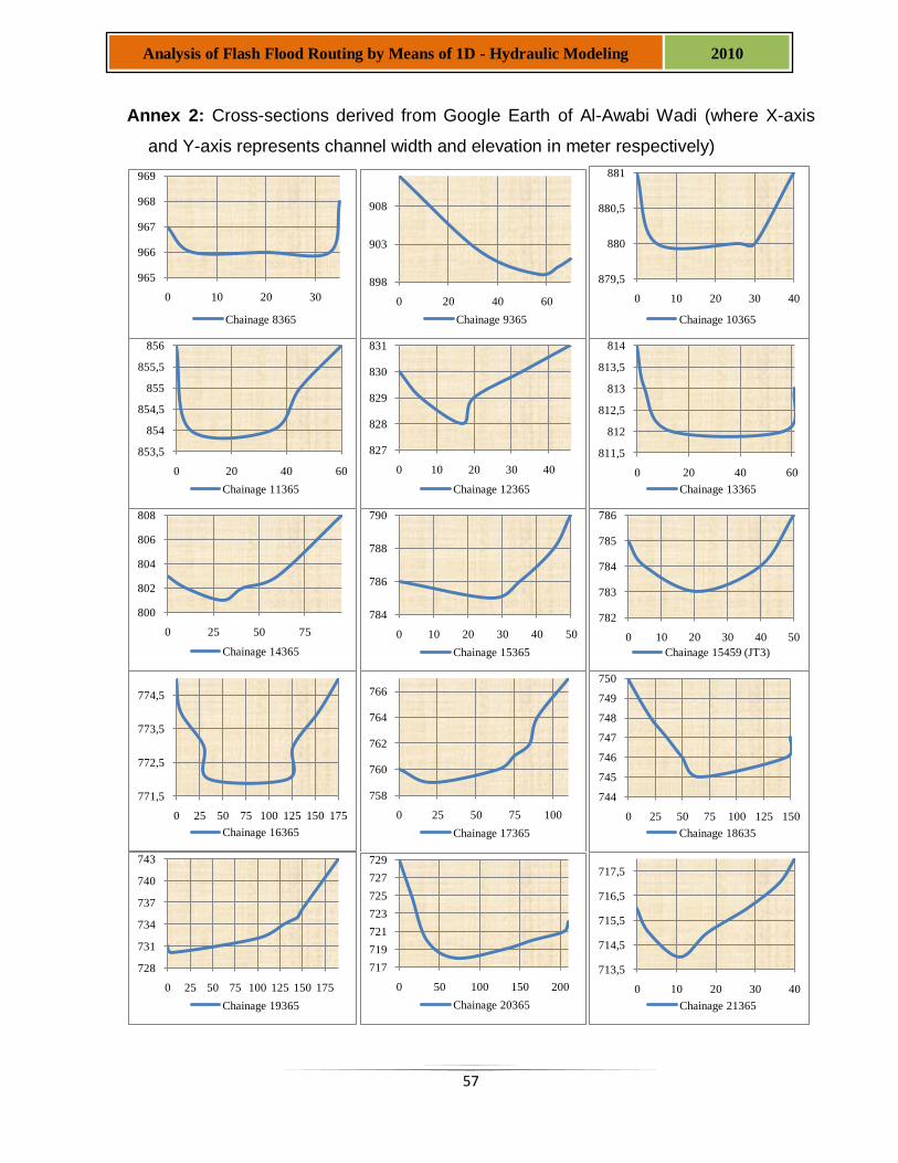
57
Analysis of Flash Flood Routing by Means of 1D - Hydraulic Modeling 2010
Annex 2: Cross-sections derived from Google Earth of Al-Awabi Wadi (where X-axis
and Y-axis represents channel width and elevation in meter respectively)
965
966
967
968
969
0 10 20 30
Chainage 8365
898
903
908
0 20 40 60
Chainage 9365
879,5
880
880,5
881
0 10 20 30 40
Chainage 10365
853,5
854
854,5
855
855,5
856
0 20 40 60
Chainage 11365
827
828
829
830
831
0 10 20 30 40
Chainage 12365
811,5
812
812,5
813
813,5
814
0 20 40 60
Chainage 13365
800
802
804
806
808
0 25 50 75
Chainage 14365
784
786
788
790
0 10 20 30 40 50
Chainage 15365
782
783
784
785
786
0 10 20 30 40 50
Chainage 15459 (JT3)
771,5
772,5
773,5
774,5
0 25 50 75 100 125 150 175
Chainage 16365
758
760
762
764
766
0 25 50 75 100
Chainage 17365
744
745
746
747
748
749
750
0 25 50 75 100 125 150
Chainage 18635
728
731
734
737
740
743
0 25 50 75 100 125 150 175
Chainage 19365
717
719
721
723
725
727
729
0 50 100 150 200
Chainage 20365
713,5
714,5
715,5
716,5
717,5
0 10 20 30 40
Chainage 21365
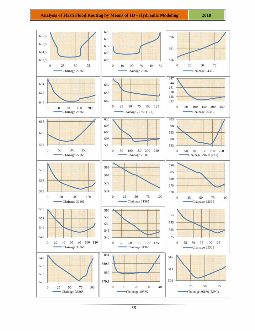
58
Analysis of Flash Flood Routing by Means of 1D - Hydraulic Modeling 2010
693,5
694,5
695,5
696,5
0 25 50 75
Chainage 22365
675
676
677
678
679
0 10 20 30 40 50
Chainage 23365
656
661
666
0 25 50 75
Chainage 24365
644
649
654
0 50 100 150 200
Chainage 25365
640
645
650
0 25 50 75 100 125
Chainage 25785 (TJ2)
632
635
638
641
644
647
0 50 100 150 200 250
Chainage 26365
595
605
615
0 50 100 150
Chainage 27365
590
595
600
605
610
0 50 100 150 200 250
Chainage 28365
583
588
593
598
603
0 50 100 150 200 250
Chainage 29660 (JT1)
578
588
598
0 50 100 150
Chainage 30365
574
579
584
589
0 25 50 75 100
Chainage 31365
570
575
580
585
590
0 25 50 75 100
Chainage 32365
547
549
551
553
0 20 40 60 80 100 120
Chainage 33365
540
545
550
555
560
0 25 50 75 100 125
Chainage 34365
525
535
545
555
0 25 50 75 100 125
Chainage 35365
528
533
538
543
0 25 50 75 100
Chainage 36365
879,5
880
880,5
881
0 10 20 30 40
Chainage 10365
506
511
516
0 25 50 75
Chainage 36630 (DBC)
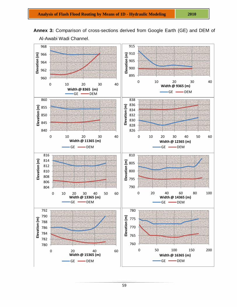
59
Analysis of Flash Flood Routing by Means of 1D - Hydraulic Modeling 2010
Annex 3: Comparison of cross-sections derived from Google Earth (GE) and DEM of
Al-Awabi Wadi Channel.
960
962
964
966
968
0 10 20 30 40
Elev
atio
n (m
)
Width @ 8365 (m)GE DEM
895
900
905
910
915
0 10 20 30 40
Elev
atio
n (m
)
Width @ 9365 (m)
GE DEM
840
845
850
855
860
0 10 20 30 40
Elev
atio
n (m
)
Width @ 11365 (m)
GE DEM
826
828
830
832
834
836
838
0 10 20 30 40 50 60
Elev
atio
n (m
)
Width @ 12365 (m)
GE DEM
804
806
808
810
812
814
816
0 10 20 30 40 50 60
Elev
atio
n (m
)
Width @ 13365 (m)GE DEM
790
795
800
805
810
0 20 40 60 80 100
Elev
atio
n (m
)
Width @ 14365 (m)
GE DEM
780
782
784
786
788
790
792
0 20 40 60
Elev
atio
n (m
)
Width @ 15365 (m)
GE DEM
760
765
770
775
780
0 50 100 150 200
Elev
atio
n (m
)
Width @ 16365 (m)
GE DEM
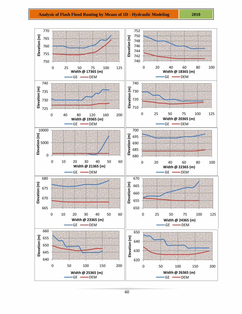
60
Analysis of Flash Flood Routing by Means of 1D - Hydraulic Modeling 2010
750
755
760
765
770
0 25 50 75 100 125
Ele
vati
on
(m)
Width @ 17365 (m)
GE DEM
740
742
744
746
748
750
752
0 20 40 60 80 100
Elev
atio
n (m
)
Width @ 18365 (m)
GE DEM
725
730
735
740
0 40 80 120 160 200
Ele
vati
on
(m)
Width @ 19365 (m)GE DEM
710
720
730
740
0 25 50 75 100 125
Ele
vati
on
(m)
Width @ 20365 (m)
GE DEM
0
5000
10000
0 10 20 30 40 50 60
Ele
vati
on
(m)
Width @ 21365 (m)
GE DEM
680
685
690
695
700
0 20 40 60 80 100
Elev
atio
n (m
)
Width @ 22365 (m)
GE DEM
665
670
675
680
0 10 20 30 40 50 60
Elev
atio
n (m
)
Width @ 23365 (m)
GE DEM
650
655
660
665
670
0 25 50 75 100 125
Elev
atio
n (m
)
Width @ 24365 (m)GE DEM
640
645
650
655
660
0 50 100 150 200
Elev
atio
n (m
)
Width @ 25365 (m)GE DEM
620
630
640
650
0 50 100 150 200
Ele
vati
on
(m)
Width @ 26365 (m)GE DEM
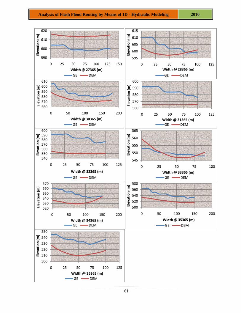
61
Analysis of Flash Flood Routing by Means of 1D - Hydraulic Modeling 2010
590
600
610
620
0 25 50 75 100 125 150
Elev
atio
n (m
)
Width @ 27365 (m)
GE DEM
595
600
605
610
615
0 25 50 75 100 125
Elev
atio
n (m
)
Width @ 28365 (m)
GE DEM
560
570
580
590
600
610
0 50 100 150 200
Ele
vati
on
(m)
Width @ 30365 (m)
GE DEM
560
570
580
590
600
0 25 50 75 100 125
Ele
vati
on
(m)
Width @ 31365 (m)GE DEM
540550560570580590600
0 25 50 75 100 125
Elev
atio
n (m
)
Width @ 32365 (m)
GE DEM
545
550
555
560
565
0 25 50 75 100
Elev
atio
n (m
)
Width @ 33365 (m)
GE DEM
520530540550560570
0 50 100 150 200
Ele
vati
on
(m)
Width @ 34365 (m)GE DEM
500
520
540
560
580
0 50 100 150 200
Elev
atio
n (m
)
Width @ 35365 (m)
GE DEM
500
510
520
530
540
550
0 25 50 75 100 125
Elev
atio
n (m
)
Width @ 36365 (m)
GE DEM

![[PPT]Chapter Four Flood Routing - Kean University | World …csmart/Hydrology/Lectures/Lecture 15u Flood... · Web viewTitle Chapter Four Flood Routing Author Chuck Last modified](https://img.pdfslide.us/doc/110x75/5b43ab4d7f8b9a2d328b746c/pptchapter-four-flood-routing-kean-university-world-csmarthydrologylectureslecture.jpg)