arX

iv:1

806.

0854

7v1

[cs

.NE

] 2

2 Ju

n 20

18

Analysis of Evolutionary Algorithms in Dynamic

and Stochastic Environments

Vahid Roostapour Mojgan Pourhassan Frank Neumann

Optimisation and Logistics

School of Computer Science

The University of Adelaide

Australia

June 25, 2018

Abstract

Many real-world optimization problems occur in environments that

change dynamically or involve stochastic components. Evolutionary al-

gorithms and other bio-inspired algorithms have been widely applied to

dynamic and stochastic problems. This survey gives an overview of major

theoretical developments in the area of runtime analysis for these prob-

lems. We review recent theoretical studies of evolutionary algorithms and

ant colony optimization for problems where the objective functions or the

constraints change over time. Furthermore, we consider stochastic prob-

lems under various noise models and point out some directions for future

research.

1

Contents

1 Introduction 3

2 Preliminaries 4

2.1 Dynamic OneMax Problem . . . . . . . . . . . . . . . . . . . . . 42.2 Linear Pseudo-Boolean Functions Under Dynamic Uniform Con-

straints . . . . . . . . . . . . . . . . . . . . . . . . . . . . . . . . 52.3 Dynamic Vertex Cover Problem . . . . . . . . . . . . . . . . . . . 62.4 Dynamic Makespan Scheduling Problem . . . . . . . . . . . . . . 62.5 Stochastic Problems and Noise Models . . . . . . . . . . . . . . . 72.6 Evolutionary algorithms . . . . . . . . . . . . . . . . . . . . . . . 7

3 Analysis of Evolutionary Algorithms on Dynamic Problems 9

3.1 OneMax Under Dynamic Uniform Constraints . . . . . . . . . . 103.2 Linear Pseudo-Boolean Functions Under Dynamic Uniform Con-

straints . . . . . . . . . . . . . . . . . . . . . . . . . . . . . . . . 153.3 The Vertex Cover Problem . . . . . . . . . . . . . . . . . . . . . 163.4 Makespan Scheduling . . . . . . . . . . . . . . . . . . . . . . . . . 183.5 The MAZE Problem . . . . . . . . . . . . . . . . . . . . . . . . . 20

4 Analysis of Evolutionary Algorithms on Stochastic Problems 22

4.1 Influence of The Population Size . . . . . . . . . . . . . . . . . . 234.2 Influence of Different Noise Distributions on The Performance of

Population Based EAs . . . . . . . . . . . . . . . . . . . . . . . . 254.3 Resampling Approach for Noisy Discrete Problems . . . . . . . . 27

5 Ant Colony Optimization 29

5.1 Dynamic Problems . . . . . . . . . . . . . . . . . . . . . . . . . . 295.2 Stochastic Problems . . . . . . . . . . . . . . . . . . . . . . . . . 30

6 Conclusions 31

2

1 Introduction

Real-world problems are often stochastic and have dynamic components. Evo-lutionary algorithms and other bio-inspired algorithmic approaches such as antcolony optimization have been applied to a wide range of stochastic and dy-namic problems. The goal of this chapter is to give an overview on recenttheoretical developments in the area of evolutionary computation for stochasticand dynamic problems in the context of discrete optimization.

Stochastic problems occur frequently in real-world applications due to un-predictable factors. A good example is the scheduling of trains. Schedules giveprecise timing when trains arrive and depart. However, the actual departureand arrival times may be subject to delays due to various factors such as weatherconditions and interfering schedules of other trains. Using evolutionary com-putation for the optimization of stochastic problems, the uncertainty is usuallyreflected through a noisy fitness function. The underlying fitness function forthese problems is noisy in the sense that it produces different results for thesame input. Two major noise models, namely prior noise and posterior noise,have been introduced and investigated in the literature. In the case of priornoise, the solution is changed prior to the evaluation of the given fitness func-tion, whereas in the case of posterior noise the solution is evaluated with thegiven fitness function and a value according to a given noise distribution is addedbefore returning the fitness value.

Dynamic problems constitute another important part occurring in real-worldapplications. Problems can change over time due to different components be-coming unavailable or available at a later point in time. Different parts of theproblem that can be subject to a change are the objective function and possi-ble constraints of the given problem. In terms of scheduling of trains, trainsmight become unavailable due to mechanical failures and it might be necessaryto reschedule the trains in the network in order to still serve the demands of thecustomers well.

The area of runtime analysis has contributed many interesting studies tothe theoretical understanding of bio-inspired algorithms in this area. We startby investigating popular benchmark algorithms such as randomized local search(RLS) and (1+1) EA on different dynamic problems. This includes dynamic ver-sions of OneMax, the classical vertex cover problem, the makespan schedulingproblem, and problem classes of the well-known knapsack problem. Afterwards,we summarize main results for stochastic problems. Important studies in thisarea consider the OneMax problem and investigate the runtime behavior ofevolutionary algorithms with respect to prior and posterior noise. Moreover,the influence of populations in evolutionary algorithms for solving stochasticproblems is analyzed in the literature, and we place a particular emphasis onthose studies. Furthermore, we review the performance of the population basedalgorithms on different posterior noise functions.

Ant colony optimization (ACO) algorithms are another important type ofbio-inspired algorithms that has been used and analyzed for solving dynamic andstochastic problems. Due to their different way of constructing solutions, based

3

on sampling from the underlying search space by performing random walks on aso-called construction graph, they have a different ability to deal with dynamicand stochastic problems. Furthermore, an important parameter in ACO algo-rithms is the pheromone update strength which allows to determine how quicklypreviously good solutions are forgotten by the algorithms. This parameter playsa crucial role when distinguishing ACO algorithms from classical evolutionaryalgorithms. At the end of this chapter, we present a summary of the obtainedresults on the dynamic and stochastic problems in the context of ACO.

This chapter is organized as follows. In Section 2, we summarize the dynamicand stochastic settings that have been investigated in the literature. We presentthe main results obtain for evolutionary algorithms in dynamic environmentsand stochastic environments in Section 3 and 4, respectively. We highlight the-oretical results on the behavior of ACO algorithms for dynamic and stochasticproblems in Section 5. Finally, we finish with some conclusions and outline somefuture research directions.

2 Preliminaries

This section includes the formal definitions of dynamic and stochastic optimiza-tion settings that are investigated in this chapter.

In dynamically changing optimization problems, some part of the problemis subject to change over time. Usually changes to the objective function orthe constraints of the given problem are considered. The different problemsthat have been studied from a theoretical perspective will be introduced in theforthcoming subsections. In the case of stochastic optimization problems, theoptimization algorithm does not have access to the deterministic fitness valueof a candidate solution. Different types of noise that change the actual fitnessvalue have been introduced. The most important ones, prior noise and posteriornoise, will be introduced in Section 2.5.

The theoretical analysis of evolutionary algorithms for dynamic and stochas-tic problems concentrates on the classical algorithms such as randomized localsearch (RLS) and (1 + 1) EA. Furthermore, the benefit of population-based ap-proaches has been examined. These algorithms will be introduced in Section 2.6.

2.1 Dynamic OneMax Problem

Investigations have started by considering a generalization of the the classicalOneMax problem. In the OneMax problem, the number of ones in the solutionis the objective to be maximized. Droste [9] has interpreted this problem asmaximizing the number of bits that match a given objective bit-string. Basedon this, he has introduced the dynamic OneMax problem, in which dynamicchanges happen on the objective bit-string over time. An extended version ofthis problem is defined by Kotzing et al. [27] where not only bit-strings areallowed. Here each position can take on integer values in 0, . . . , r − 1 forr ∈ N≥2. The formal definition of the problem follows.

4

Let [r] = 0, . . . , r−1 for r ∈ N≥2, and x, y ∈ [r]. Moreover, let the distancebetween x and y be

d(x, y) = min (x− y) mod r, (y − x) mod r .

The extended OneMax problem, OneMaxa : [r]n → R, where a is theobjective string defining the optimum, is given as:

OneMaxa(x) =

n∑

i=1

d(ai, xi).

The goal is to find and maintain a solution with minimum value of OneMaxa.Given a probability value p, the dynamism that is defined on this problem is

to change each component i, 1 ≤ i ≤ n, of the optimal solution a independentlyas:

ai =

ai + 1 mod r; with probability p/2ai − 1 mod r; with probability p/2ai; with probability 1− p

2.2 Linear Pseudo-Boolean Functions Under Dynamic Uni-

form Constraints

Linear pseudo-Boolean functions play a key role in the runtime analysis of evo-lutionary algorithms. Let x = x1x2 . . . xn be a search point in search space0, 1n, and wi, 1 ≤ i ≤ n positive real weights. A linear pseudo-Booleanfunction f(x) is defined as:

f(x) = w0 +

n∑

i=1

wixi.

For simplicity and as done in most studies, we assume w0 = 0 in the follow-ing. The optimization of a linear objective function under a linear constraint isequivalent to the classical knapsack problem [26]. The optimization of a linearobjective function together with a uniform constraint has recently been inves-tigated in the static setting [15]. Given a bound B, 0 ≤ B ≤ n, a solution x isfeasible if the number of 1-bits of the search point x is at most B. The boundB is also known as the cardinality bound. We denote the number of 1-bits ofx by |x|1 =

∑ni=1 xi. The formal definition for maximizing a pseudo-Boolean

linear function under a cardinality bound constraint is given by:

max f(x)

s.t. |x|1 ≤ B.

The dynamic version of this problem, referred to as the problem with adynamic uniform constraint, is defined in [39]. Here the cardinality bound

5

changes from B to some new value B∗. Starting from a solution that is optimalfor the bound B, the problem is then to find an optimal solution for B∗. There-optimization time of an evolutionary algorithm is defined as the number offitness evaluations that is required to find the new optimal solution.

2.3 Dynamic Vertex Cover Problem

The vertex cover problem is one of the best-known NP-hard combinatorial op-timization problems. Given a graph G = (V, E), where V = v1, . . . , vn is theset of vertices and E = e1, . . . , em is the set of edges, the goal is to find a min-imum subset of nodes VC ⊆ V that covers all edges in E, i.e. ∀e ∈ E, e∩VC 6= ∅.In the dynamic version of the problem, an edge can be added to or deleted fromthe graph.

As the vertex cover problem is NP-hard, it has been mainly studied in termsof approximations. The problem can be approximated within a worst caseapproximation ratio of 2 by various algorithms. One standard approach toobtain a 2-approximation is to compute a maximal matching and take all nodesadjacent to the chosen matching edges for the vertex cover. Starting from asolution that is a 2-approximation for the current instance of the problem, in thedynamic version of the problem the goal is to obtain a 2-approximate solutionfor that instance of the problem after one dynamic change. The re-optimizationtime for this problem refers to the required time for the investigated algorithmto find a 2-approximate solution for the new instance. This dynamic setting hasbeen investigated in [36].

2.4 Dynamic Makespan Scheduling Problem

The makespan scheduling problem can be defined as follows. Given n jobs andtheir processing times pi > 0, 1 ≤ i ≤ n, the goal is to assign each job to one oftwo machines M1 and M2 such that the makespan is minimized. The makespanis the time that the busier machine takes to finish all assigned jobs. A solutionis represented by a vector x ∈ 0, 1n which means that job i is assigned tomachine M1 if xi = 0 and it is assigned to M2 if xi = 1, 1 ≤ i ≤ n. With thisrepresentation, the makespan of a given solution x is given by

f(x) = max

n∑

i=1

pi(1− xi),

n∑

i=1

pixi

and the goal is to minimize f . In the dynamic version of this problem, theprocessing time of a job may change over time, but stays within a given interval.In [34], the setting pi ∈ [L, U ], 1 ≤ i ≤ n, where L and U are a lower andupper bound on each processing time, have been investigated. The analysisconcentrates on the time evolutionary algorithms need to produce a solutionwhere the two machines have discrepancy at most U . Dynamic changes to theprocessing times of the jobs have been investigated in two different settings. Inthe first setting, an adversary is allowed to change the processing time of exactly

6

one job. In the second setting, the job to be changed is picked by an adversarybut the processing time of a job is altered randomly.

2.5 Stochastic Problems and Noise Models

We consider stochastic optimization problems where the fitness function is sub-ject to some noise. Two different noise models have mainly been studied inthe area of the theoretical analysis of evolutionary computation. Noises thataffect the solution before the evaluation are called prior noise. In this case, thefitness function returns the fitness value of a solution that may differ from thegiven solution because of the noise. Droste studied the effect of a prior noisewhich flips one randomly chosen bit of the given solution with probability of p,before each evaluation [11]. Note that the noise does not change the solution,but it causes the fitness function to evaluate a solution with a noisy bit flip.Other kinds of prior noises have also been considered. For example, a priornoise which flips each bits with the probability of p or a prior noise which setseach bit independently with probability of p to 0 [22].

Another important type of noise is where the fitness of the solution is changedafter evaluation. This type of noise is called posterior noise or additive posteriornoise. The noise which commonly comes from a defined distribution D, addsthe value of a random variable sampled from D to the value coming from theoriginal fitness function [20, 13, 22].

In the noisy environment, the problem of finding the optimal solutions isharder as the noise is misleading the search. The goal is to find an optimalsolution for the original non noisy fitness function by evaluating solutions onthe fitness function affected by noise. However, it has been proven that sim-ple evolutionary algorithms behave considerably well when facing this kind ofproblems. In addition to this, properties of stochastic settings that are hard forevolutionary algorithms to deal with have also been studied in [13].

We concentrate on stochastic problems with a fixed and known solutionlength that are subject to noise. We would like to mention that there are alsostudies investigating the performance of evolutionary algorithms with unknownsolution length. This poses a different type of uncertainty which we will notcapture in this chapter. We refer the interesting reader to [3, 6].

2.6 Evolutionary algorithms

Analyzing evolutionary algorithms often starts by investigating a standard ran-domized local search approach and a simple (1 + 1) EA. Here we present thesealgorithms in addition to a population-based (µ + λ) EA for which results aresummarized in Section 4.

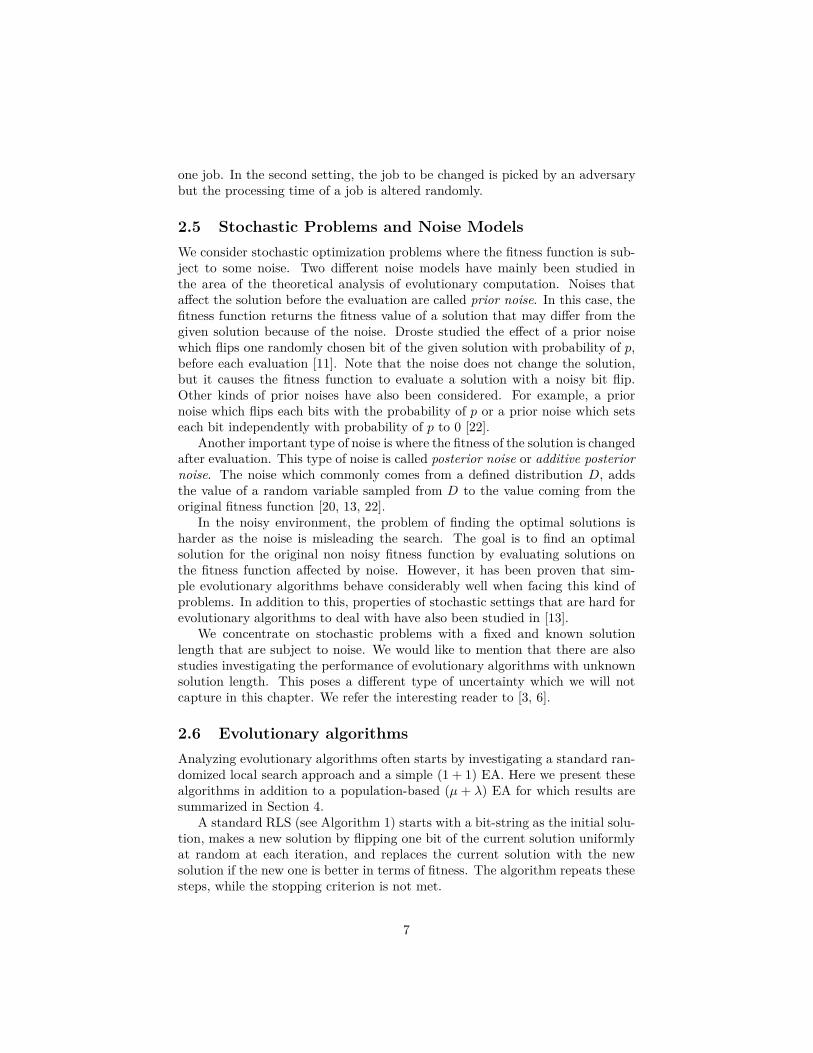
A standard RLS (see Algorithm 1) starts with a bit-string as the initial solu-tion, makes a new solution by flipping one bit of the current solution uniformlyat random at each iteration, and replaces the current solution with the newsolution if the new one is better in terms of fitness. The algorithm repeats thesesteps, while the stopping criterion is not met.

7

Algorithm 1: RLS

1 The initial solution x is given;2 while stopping criterion not met do

3 y ← flip one bit of x chosen uniformly at random;4 if f(y) ≥ f(x) then

5 x← y;

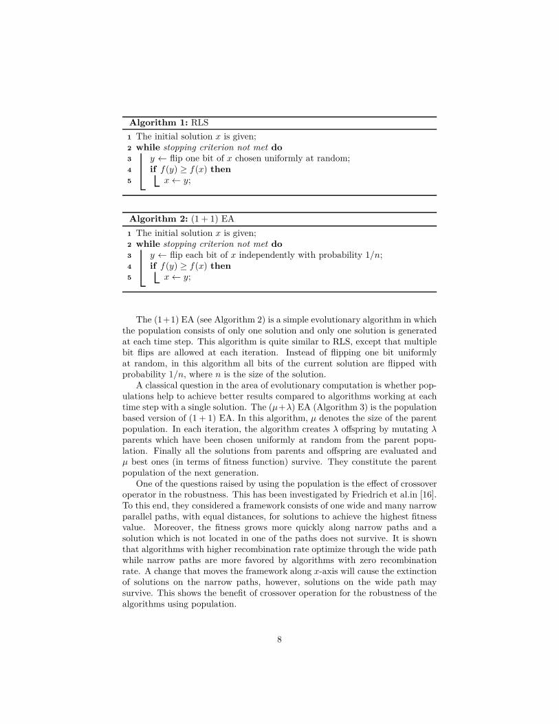
Algorithm 2: (1 + 1) EA

1 The initial solution x is given;2 while stopping criterion not met do

3 y ← flip each bit of x independently with probability 1/n;4 if f(y) ≥ f(x) then

5 x← y;

The (1+1) EA (see Algorithm 2) is a simple evolutionary algorithm in whichthe population consists of only one solution and only one solution is generatedat each time step. This algorithm is quite similar to RLS, except that multiplebit flips are allowed at each iteration. Instead of flipping one bit uniformlyat random, in this algorithm all bits of the current solution are flipped withprobability 1/n, where n is the size of the solution.

A classical question in the area of evolutionary computation is whether pop-ulations help to achieve better results compared to algorithms working at eachtime step with a single solution. The (µ+λ) EA (Algorithm 3) is the populationbased version of (1 + 1) EA. In this algorithm, µ denotes the size of the parentpopulation. In each iteration, the algorithm creates λ offspring by mutating λparents which have been chosen uniformly at random from the parent popu-lation. Finally all the solutions from parents and offspring are evaluated andµ best ones (in terms of fitness function) survive. They constitute the parentpopulation of the next generation.

One of the questions raised by using the population is the effect of crossoveroperator in the robustness. This has been investigated by Friedrich et al.in [16].To this end, they considered a framework consists of one wide and many narrowparallel paths, with equal distances, for solutions to achieve the highest fitnessvalue. Moreover, the fitness grows more quickly along narrow paths and asolution which is not located in one of the paths does not survive. It is shownthat algorithms with higher recombination rate optimize through the wide pathwhile narrow paths are more favored by algorithms with zero recombinationrate. A change that moves the framework along x-axis will cause the extinctionof solutions on the narrow paths, however, solutions on the wide path maysurvive. This shows the benefit of crossover operation for the robustness of thealgorithms using population.

8

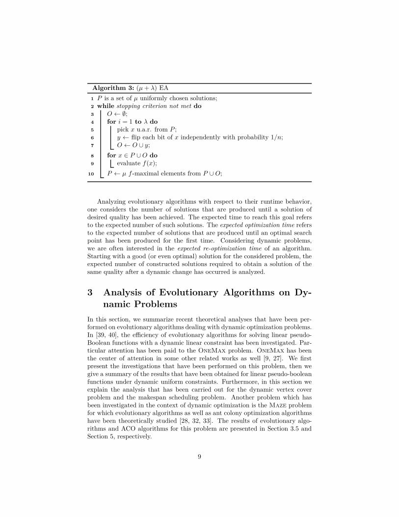
Algorithm 3: (µ + λ) EA

1 P is a set of µ uniformly chosen solutions;2 while stopping criterion not met do

3 O ← ∅;4 for i = 1 to λ do

5 pick x u.a.r. from P ;6 y ← flip each bit of x independently with probability 1/n;7 O ← O ∪ y;

8 for x ∈ P ∪O do

9 evaluate f(x);

10 P ← µ f -maximal elements from P ∪O;

Analyzing evolutionary algorithms with respect to their runtime behavior,one considers the number of solutions that are produced until a solution ofdesired quality has been achieved. The expected time to reach this goal refersto the expected number of such solutions. The expected optimization time refersto the expected number of solutions that are produced until an optimal searchpoint has been produced for the first time. Considering dynamic problems,we are often interested in the expected re-optimization time of an algorithm.Starting with a good (or even optimal) solution for the considered problem, theexpected number of constructed solutions required to obtain a solution of thesame quality after a dynamic change has occurred is analyzed.

3 Analysis of Evolutionary Algorithms on Dy-

namic Problems

In this section, we summarize recent theoretical analyses that have been per-formed on evolutionary algorithms dealing with dynamic optimization problems.In [39, 40], the efficiency of evolutionary algorithms for solving linear pseudo-Boolean functions with a dynamic linear constraint has been investigated. Par-ticular attention has been paid to the OneMax problem. OneMax has beenthe center of attention in some other related works as well [9, 27]. We firstpresent the investigations that have been performed on this problem, then wegive a summary of the results that have been obtained for linear pseudo-booleanfunctions under dynamic uniform constraints. Furthermore, in this section weexplain the analysis that has been carried out for the dynamic vertex coverproblem and the makespan scheduling problem. Another problem which hasbeen investigated in the context of dynamic optimization is the Maze problemfor which evolutionary algorithms as well as ant colony optimization algorithmshave been theoretically studied [28, 32, 33]. The results of evolutionary algo-rithms and ACO algorithms for this problem are presented in Section 3.5 andSection 5, respectively.

9

3.1 OneMax Under Dynamic Uniform Constraints

The first runtime analysis of evolutionary algorithms for a dynamic discreteproblem has been presented by Droste [9]. In that article, the OneMax prob-lem is considered and the goal is to find a solution which has the minimumHamming distance to an objective bit-string. A dynamic change in that workis changing one bit of the objective bit-string, which happens at each time stepwith probability p′ and results in the dynamic changes of the fitness functionover time. Droste has found the maximum rate of the dynamic changes suchthat the expected optimization time of (1 + 1) EA remains polynomial for thestudied problem. More precisely, he has proved that (1+1) EA has a polynomialexpected runtime if p′ = O(log(n)/n), while for every substantially larger proba-bility the runtime becomes super polynomial. It is worth noting that the resultsof that article hold even if the expected re-optimization time of the problem islarger than the expected time until the next dynamic change happens.

Using drift analysis, Kotzing et al. [27] have reproved some of the resultsin [9]. Furthermore, they have carried out theoretical investigations for theextended dynamic OneMax problem (see Section 2.1), in which each variablecan take on more than two values. They also carried out an anytime analysis(introduced in [24]) and show how closely their investigated algorithm can trackthe dynamically moving target over time.

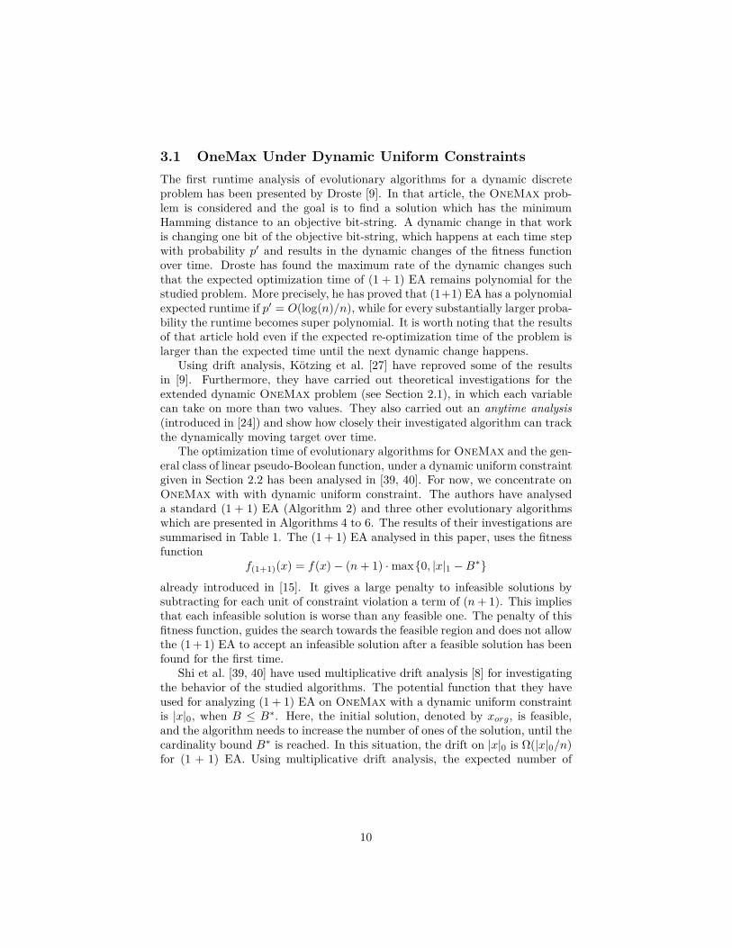
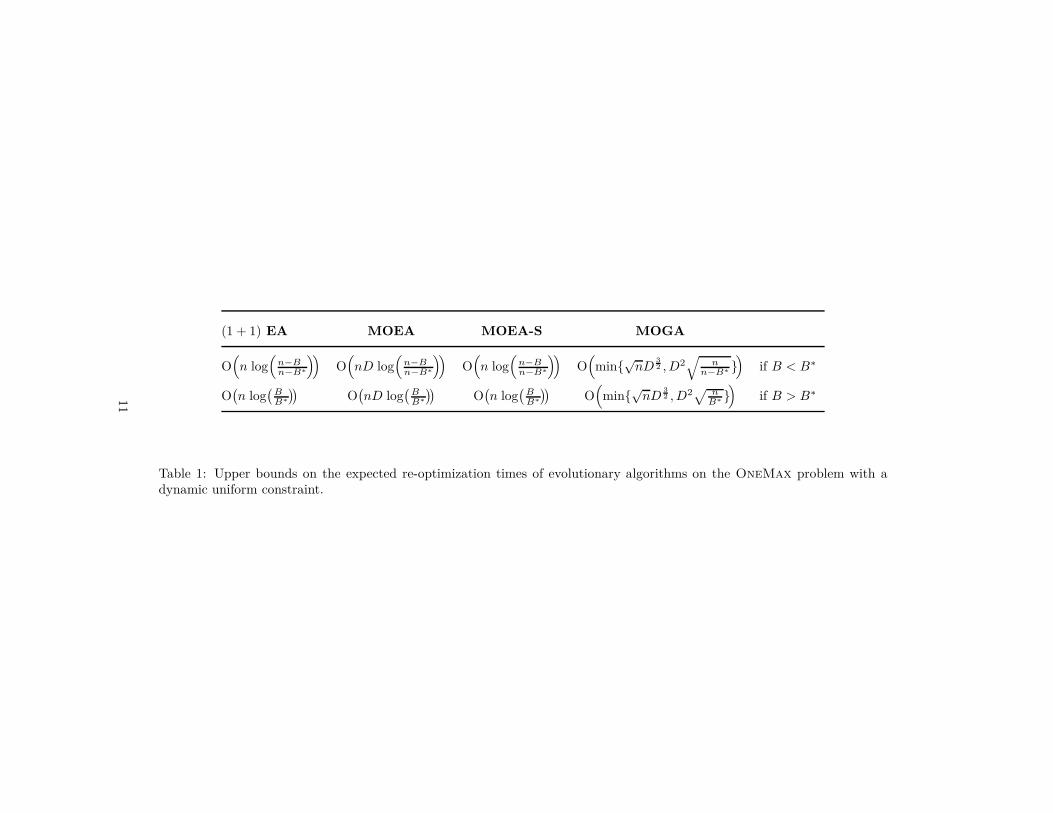
The optimization time of evolutionary algorithms for OneMax and the gen-eral class of linear pseudo-Boolean function, under a dynamic uniform constraintgiven in Section 2.2 has been analysed in [39, 40]. For now, we concentrate onOneMax with with dynamic uniform constraint. The authors have analyseda standard (1 + 1) EA (Algorithm 2) and three other evolutionary algorithmswhich are presented in Algorithms 4 to 6. The results of their investigations aresummarised in Table 1. The (1 + 1) EA analysed in this paper, uses the fitnessfunction

f(1+1)(x) = f(x)− (n + 1) ·max0, |x|1 −B∗already introduced in [15]. It gives a large penalty to infeasible solutions bysubtracting for each unit of constraint violation a term of (n + 1). This impliesthat each infeasible solution is worse than any feasible one. The penalty of thisfitness function, guides the search towards the feasible region and does not allowthe (1 + 1) EA to accept an infeasible solution after a feasible solution has beenfound for the first time.

Shi et al. [39, 40] have used multiplicative drift analysis [8] for investigatingthe behavior of the studied algorithms. The potential function that they haveused for analyzing (1 + 1) EA on OneMax with a dynamic uniform constraintis |x|0, when B ≤ B∗. Here, the initial solution, denoted by xorg, is feasible,and the algorithm needs to increase the number of ones of the solution, until thecardinality bound B∗ is reached. In this situation, the drift on |x|0 is Ω(|x|0/n)for (1 + 1) EA. Using multiplicative drift analysis, the expected number of

10

(1 + 1) EA MOEA MOEA-S MOGA

O(

n log(

n−Bn−B∗

))

O(

nD log(

n−Bn−B∗

))

O(

n log(

n−Bn−B∗

))

O(

min√nD3

2 , D2√

nn−B∗

)

if B < B∗

O(

n log(

BB∗

))

O(

nD log(

BB∗

))

O(

n log(

BB∗

))

O(

min√nD3

2 , D2√

nB∗)

if B > B∗

Table 1: Upper bounds on the expected re-optimization times of evolutionary algorithms on the OneMax problem with adynamic uniform constraint.

11

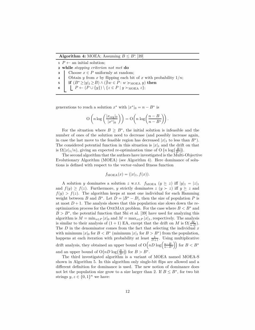
Algorithm 4: MOEA; Assuming B ≤ B∗. [39]

1 P ← an initial solution;2 while stopping criterion not met do

3 Choose x ∈ P uniformly at random;4 Obtain y from x by flipping each bit of x with probability 1/n;5 if (B∗≥|y|1≥B) ∧ (∄w ∈ P : w <MOEA y) then

6 P ← (P ∪ y) \ z ∈ P | y ≻MOEA z;

generations to reach a solution x∗ with |x∗|0 = n−B∗ is

O

(

n log

( |xorg|0|x∗|0

))

= O

(

n log

(

n−B

n−B∗

))

.

For the situation where B ≥ B∗, the initial solution is infeasible and thenumber of ones of the solution need to decrease (and possibly increase again,in case the last move to the feasible region has decreased |x|1 to less than B∗).The considered potential function in this situation is |x|1 and the drift on thatis Ω(|x|1/n), giving an expected re-optimization time of O

(

n log(

BB∗

))

.The second algorithm that the authors have investigated is the Multi-Objective

Evolutionary Algorithm (MOEA) (see Algorithm 4). Here dominance of solu-tions is defined with respect to the vector-valued fitness function

fMOEA(x) = (|x|1, f(x)).

A solution y dominates a solution z w.r.t. fMOEA (y z) iff |y|1 = |z|1and f(y) ≥ f(z). Furthermore, y strictly dominates z (y ≻ z) iff y z andf(y) > f(z). The algorithm keeps at most one individual for each Hammingweight between B and B∗. Let D = |B∗ −B|, then the size of population P isat most D + 1. The analysis shows that this population size slows down the re-optimization process for the OneMax problem. For the case where B < B∗ andB > B∗, the potential function that Shi et al. [39] have used for analyzing thisalgorithm is M = minx∈P |x|0 and M = maxx∈P |x|1, respectively. The analysisis similar to their analysis of (1 + 1) EA, except that the drift on M is Ω( M

n·D ).The D in the denominator comes from the fact that selecting the individual xwith minimum |x|0 for B < B∗ (minimum |x|1 for B > B∗) from the population,happens at each iteration with probability at least 1

D+1 . Using multiplicative

drift analysis, they obtained an upper bound of O(

nD log(

n−Bn−B∗

))

for B < B∗

and an upper bound of O(

nD log(

BB∗

))

for B > B∗.The third investigated algorithm is a variant of MOEA named MOEA-S

shown in Algorithm 5. In this algorithm only single-bit flips are allowed and adifferent definition for dominance is used. The new notion of dominance doesnot let the population size grow to a size larger than 2. If B ≤ B∗, for two bitstrings y, z ∈ 0, 1n we have:

12

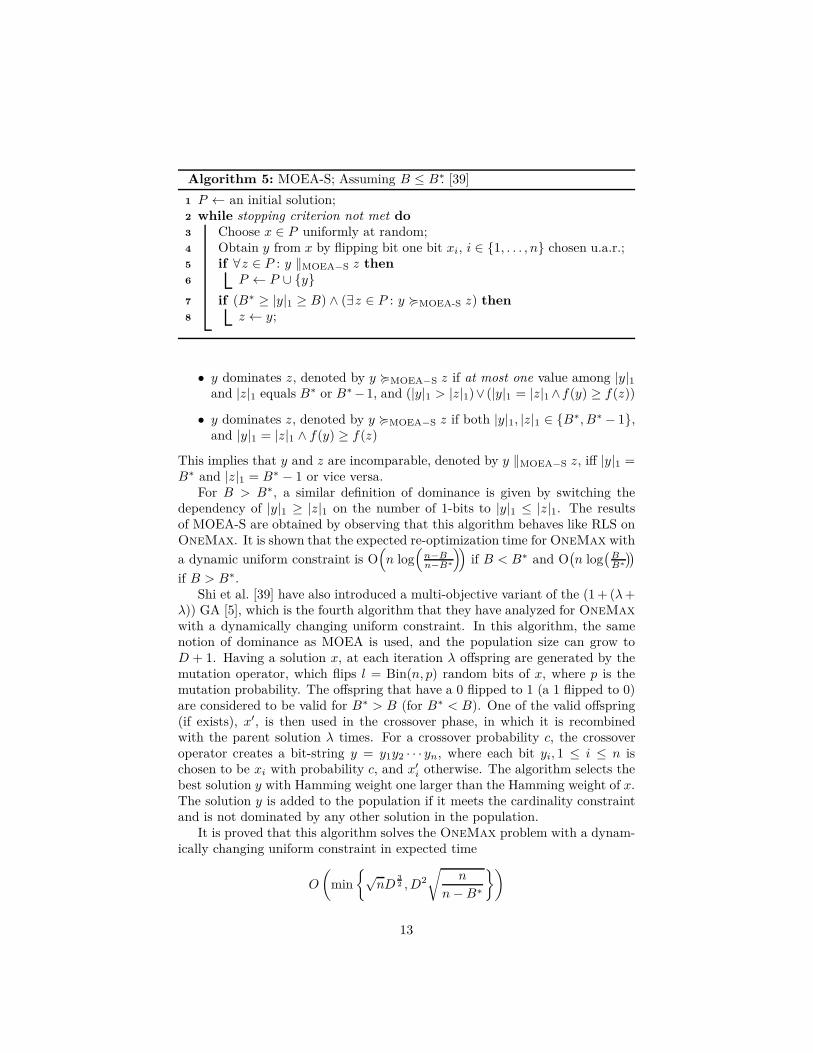
Algorithm 5: MOEA-S; Assuming B ≤ B∗. [39]

1 P ← an initial solution;2 while stopping criterion not met do

3 Choose x ∈ P uniformly at random;4 Obtain y from x by flipping bit one bit xi, i ∈ 1, . . . , n chosen u.a.r.;5 if ∀z ∈ P : y ‖MOEA−S z then

6 P ← P ∪ y7 if (B∗ ≥ |y|1 ≥ B) ∧ (∃z ∈ P : y <MOEA-S z) then

8 z ← y;

• y dominates z, denoted by y <MOEA−S z if at most one value among |y|1and |z|1 equals B∗ or B∗−1, and (|y|1 > |z|1)∨ (|y|1 = |z|1∧f(y) ≥ f(z))

• y dominates z, denoted by y <MOEA−S z if both |y|1, |z|1 ∈ B∗, B∗ − 1,and |y|1 = |z|1 ∧ f(y) ≥ f(z)

This implies that y and z are incomparable, denoted by y ‖MOEA−S z, iff |y|1 =B∗ and |z|1 = B∗ − 1 or vice versa.

For B > B∗, a similar definition of dominance is given by switching thedependency of |y|1 ≥ |z|1 on the number of 1-bits to |y|1 ≤ |z|1. The resultsof MOEA-S are obtained by observing that this algorithm behaves like RLS onOneMax. It is shown that the expected re-optimization time for OneMax with

a dynamic uniform constraint is O(

n log(

n−Bn−B∗

))

if B < B∗ and O(

n log(

BB∗

))

if B > B∗.Shi et al. [39] have also introduced a multi-objective variant of the (1 + (λ +

λ)) GA [5], which is the fourth algorithm that they have analyzed for OneMax

with a dynamically changing uniform constraint. In this algorithm, the samenotion of dominance as MOEA is used, and the population size can grow toD + 1. Having a solution x, at each iteration λ offspring are generated by themutation operator, which flips l = Bin(n, p) random bits of x, where p is themutation probability. The offspring that have a 0 flipped to 1 (a 1 flipped to 0)are considered to be valid for B∗ > B (for B∗ < B). One of the valid offspring(if exists), x′, is then used in the crossover phase, in which it is recombinedwith the parent solution λ times. For a crossover probability c, the crossoveroperator creates a bit-string y = y1y2 · · · yn, where each bit yi, 1 ≤ i ≤ n ischosen to be xi with probability c, and x′

i otherwise. The algorithm selects thebest solution y with Hamming weight one larger than the Hamming weight of x.The solution y is added to the population if it meets the cardinality constraintand is not dominated by any other solution in the population.

It is proved that this algorithm solves the OneMax problem with a dynam-ically changing uniform constraint in expected time

O

(

min

√nD

3

2 , D2

√

n

n−B∗

)

13

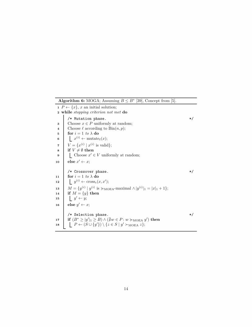
Algorithm 6: MOGA; Assuming B ≤ B∗ [39], Concept from [5].

1 P ← x, x an initial solution;2 while stopping criterion not met do

/* Mutation phase. */

3 Choose x ∈ P uniformly at random;4 Choose ℓ according to Bin(n, p);5 for i = 1 to λ do

6 x(i) ← mutateℓ(x);

7 V = x(i) | x(i) is valid;8 if V 6= ∅ then

9 Choose x′ ∈ V uniformly at random;

10 else x′ ← x;

/* Crossover phase. */

11 for i = 1 to λ do

12 y(i) ← crossc(x, x′);

13 M = y(i) | y(i) is <MOEA-maximal ∧ |y(i)|1 = |x|1 + 1;14 if M = y then

15 y′ ← y;

16 else y′ ← x;

/* Selection phase. */

17 if (B∗ ≥ |y′|1 ≥ B) ∧ (∄w ∈ P : w <MOEA y′) then

18 P ← (S ∪ y′) \ z ∈ S | y′ ≻MOEA z;

14

if p = λn , c = 1

λ , λ =√

n/(n− |x|1) for B∗ > B, and in expected time

O

(

min

√nD

3

2 , D2

√

n

B∗

)

if λ =√

n/|x|1 for B∗ < B [40]. The key argument behind these results isto show a constant probability of producing a valid offspring in the mutationphase, and then show a constant probability of generating a solution y in thecrossover phase that is the same as x except for one bit, which is flipped from0 to 1 for B∗ > B and from 1 to 0 for B∗ < B.

3.2 Linear Pseudo-Boolean Functions Under Dynamic Uni-

form Constraints

The classical (1 + 1) EA and three multi-objective evolutionary algorithms havebeen investigated in [39] for re-optimizing linear functions under dynamic uni-form constraints. The general class of linear constraints on linear problems leadsto exponential optimization times for many evolutionary algorithms [15, 43]. Shiet al. [39] considered the dynamic setting given in Section 2.2 and analyze theexpected re-optimization time of the investigated evolutionary algorithms. Thissection includes the results that they have obtained, in addition to the proofideas of their work.

The algorithms that are investigated in their work, are presented in Algo-rithms 2 to 6 of Section 3.1 and the results are summarized in Table 2. The(1 + 1) EA (Algorithm 2) uses the following fitness function which has beenintroduced by Friedrich et al. [15] (similar to the fitness function for OneMax

in Section 3.1):

f(1+1)(x) = f(x)− (nwmax + 1) ·max0, |x|1 −B∗

Here, wmax = maxni=1 wi denotes the maximum weight, and the large penalty

for constraint violations guides the search towards the feasible region.Shi et al. [39] have investigated this setting similar to the analysis of OneMax

under dynamic uniform constraints (Section 3.1). The main difference is thatfor a non-optimal solution with B∗ 1-bits, an improvement is not possible byflipping a single bit. A 2-bit flip that flips a 1 and a 0 may be required, resultingin an expected re-optimization time of O

(

n2 log(B∗ wmax))

.The second investigated algorithm, MOEA, uses the fitness function fMOEA

and the notion of dominance defined in Section 3.1. Unlike the re-optimizationtime of this algorithm for the OneMax problem, whose upper bound is worsethan the upper bound of (1 + 1) EA; for the general linear functions the upperbounds obtained for MOEA are smaller than the ones obtained for (1 + 1) EA.The reason is that the algorithm is allowed to keep one individual for eachHamming weight between the two bounds in the population. This avoids thenecessity for a 2-bit flip. To reach a solution that is optimal for cardinalityA+1, the algorithm can use the individual that is optimal for cardinality A and

15

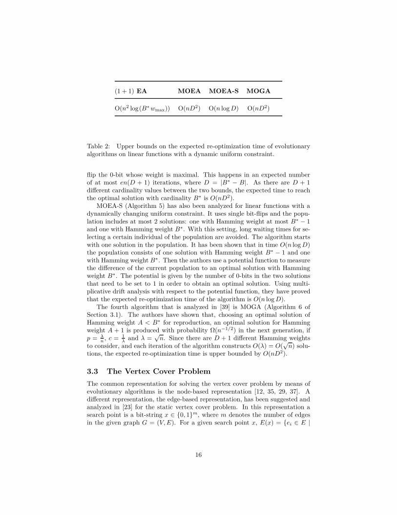
(1 + 1) EA MOEA MOEA-S MOGA

O(n2 log(B∗ wmax)) O(nD2) O(n log D) O(nD2)

Table 2: Upper bounds on the expected re-optimization time of evolutionaryalgorithms on linear functions with a dynamic uniform constraint.

flip the 0-bit whose weight is maximal. This happens in an expected numberof at most en(D + 1) iterations, where D = |B∗ − B|. As there are D + 1different cardinality values between the two bounds, the expected time to reachthe optimal solution with cardinality B∗ is O(nD2).

MOEA-S (Algorithm 5) has also been analyzed for linear functions with adynamically changing uniform constraint. It uses single bit-flips and the popu-lation includes at most 2 solutions: one with Hamming weight at most B∗ − 1and one with Hamming weight B∗. With this setting, long waiting times for se-lecting a certain individual of the population are avoided. The algorithm startswith one solution in the population. It has been shown that in time O(n log D)the population consists of one solution with Hamming weight B∗ − 1 and onewith Hamming weight B∗. Then the authors use a potential function to measurethe difference of the current population to an optimal solution with Hammingweight B∗. The potential is given by the number of 0-bits in the two solutionsthat need to be set to 1 in order to obtain an optimal solution. Using multi-plicative drift analysis with respect to the potential function, they have provedthat the expected re-optimization time of the algorithm is O(n log D).

The fourth algorithm that is analyzed in [39] is MOGA (Algorithm 6 ofSection 3.1). The authors have shown that, choosing an optimal solution ofHamming weight A < B∗ for reproduction, an optimal solution for Hammingweight A + 1 is produced with probability Ω(n−1/2) in the next generation, ifp = λ

n , c = 1λ and λ =

√n. Since there are D + 1 different Hamming weights

to consider, and each iteration of the algorithm constructs O(λ) = O(√

n) solu-tions, the expected re-optimization time is upper bounded by O(nD2).

3.3 The Vertex Cover Problem

The common representation for solving the vertex cover problem by means ofevolutionary algorithms is the node-based representation [12, 35, 29, 37]. Adifferent representation, the edge-based representation, has been suggested andanalyzed in [23] for the static vertex cover problem. In this representation asearch point is a bit-string x ∈ 0, 1m, where m denotes the number of edgesin the given graph G = (V, E). For a given search point x, E(x) = ei ∈ E |

16

xi = 1 is the set of chosen edges. The cover set induced by x, denoted byVC(x), is the set of all nodes that are adjacent to at least one edge in E(x).

Three variants of RLS and (1 + 1) EA have been investigated. This includesone node-based approach and two edge-based approaches. The node-based ap-proach and one of the edge-based approaches use a standard fitness function,

f(s) = |VC(s)|+ (|V |+ 1) · |e ∈ E|e ∩ VC(s) = ∅|,in which each uncovered edge obtains a large penalty of |V | + 1. In [23],

an exponential lower bound for finding a 2-approximate solution for the staticvertex cover problem with these two approaches using the fitness function fhas been shown. Furthermore, considering the dynamic vertex cover problem,Pourhassan et al. [36] have proved that there exist classes of instances of bipar-tite graphs where dynamic changes on the graph lead to a bad approximationbehavior.

The third variant of an evolutionary algorithm that Jansen et al. [23] haveinvestigated, is an edge-based approach with a specific fitness function. Thefitness function fe has a very large penalty for common nodes among selectededges. It is defined as

fe(s) = |VC(s)|+ (|V |+ 1) · |e ∈ E | e ∩ VC(s) = ∅|+ (|V |+ 1) · (m + 1) · |(e, e′) ∈ E(s)× E(s) | e 6= e′, e ∩ e′ 6= ∅|.

This fitness function guides the search towards a matching, and afterwards toa maximal matching. In other words, whenever the algorithms find a matching,then they do not accept a solution that is not a matching, and whenever theyfind a matching that induces a node set with k uncovered edges, then they donot accept a solution with k′ > k uncovered edges. It is well known that takingall the nodes belonging to the edges of a maximal matching for a given graphresults in a 2-approximate for the vertex cover problem.

The variant of RLS and (1 + 1) EA work with the edge-based representationand the fitness function fe. Note that search points are bit-strings of size m, andthe probability of flipping each bit in (1 + 1) EA is 1/m. Jansen et al. [23] haveproved that RLS and (1 + 1) EA with the edge-based approach find a maximalmatching which induces a 2-approximate solution for the vertex cover problemin expected time O(m log m), where m is the number of edges.

The behavior of RLS and (1 + 1) EA with this edge-based approach hasbeen investigated on the dynamic vertex cover problem (see Section 2.3) in [36].It is proved in [36] that starting from a 2-approximate solution for a currentinstance of the problem, in expected time O(m) RLS finds a 2-approximatesolution after a dynamic change of adding or deleting an edge. The authorsof that paper have investigated the situation for adding an edge and removingan edge separately. For adding an edge, they have shown that the new edge iseither already covered and the maximal matching stays a maximal matching, orit is not covered by the current edge set and the current edge set is a matchingthat induces a solution with one (only the new edge) uncovered edge. Since the

17

number of uncovered edges does not grow in this approach and the algorithmselects the only uncovered edge with probability 1/m, a maximal matching isfound in expected m steps. This argument also holds for (1 + 1) EA, but theprobability of selecting the uncovered edge and having no other mutations withthis algorithm is at least 1/(em). Therefore, the expected re-optimization timefor (1 + 1) EA after a dynamic addition is also O(m).

When an edge is deleted from the graph, if it had been selected in thesolution, a number of edges can be uncovered in the new situation. All theseuncovered edges had been covered by the two nodes of the removed edge, andcan be partitioned into two sets U1 and U2, such that all edges of each set sharea node. Therefore, if the algorithm selects one edge from each set (if any exist),the induced node set becomes a vertex cover again. It will again be a maximalmatching and therefore a 2-approximate solution. On the other hand, no otherone-bit flips in this situation can be accepted, because they either increase thenumber of uncovered edges, or make the solution become a non-matching. WithRLS, in which only one-bit flips are possible, the probabilities of selecting one

edge from U1 and U2 at each step are |U1|m and |U2|

m , respectively. Therefore, inexpected time O(m) one edge from each set is selected by the algorithm.

The analysis for (1 + 1) EA dealing with a dynamic deletion is more com-plicated, because multiple-bit flips can happen. In other words, it is possibleto deselect an edge and uncover some edges at the same step where an edgefrom U1 or U2 is being selected to cover some other edges. An upper bound ofO(m log m) is shown in [36] for the expected re-optimization time for (1+1) EAafter a dynamic deletion, which is the same as the expected time to find a 2-approximate solution with that algorithm, starting from an arbitrary solution.

3.4 Makespan Scheduling

Makespan scheduling is another problem which has been considered in a dy-namic setting [34]. It is assumed that the processing time of job i for 1 ≤ i ≤ n,is pi ∈ [L, U ], where L and U are lower and upper bounds on the processing timeof jobs respectively. In addition, the ratio between the upper bound and thelower bound is denoted by R = U/L. The runtime performance of (1 + 1) EAand RLS is studied in terms of finding a solution with a good discrepancy and itis assumed that there is no stopping criteria for the algorithms except achievingsuch a solution. The discrepancy d(x) of a solution x is defined as

d(x) =

∣

∣

∣

∣

∣

(

n∑

i=1

pi(1− xi)

)

−(

n∑

i=1

pixi

)∣

∣

∣

∣

∣

.

Note that a solution that has a smaller discrepancy also has a smaller makespan.Moreover, the proofs benefit from an important observation about the fullermachine (the machine which is loaded heavier and determines the makespan).The observation is on the minimum number of jobs of the fuller machine interms of U and L. :

18

• Every solution has at least ⌈(P/2)/U⌉ ≥ ⌈(nL/2)/U⌉ = ⌈(n/2)(L/U)⌉ =⌈(n/2)R−1)⌉ jobs on the fuller machine, where P =

∑ni=1 pi

Two dynamic settings are studied for this problem. The first one is calledthe adversary model in which a strong adversary is allowed to choose at mostone arbitrary job i in each iteration and change its processing time to a newpi ∈ [L, U ]. It is proven that, independently of initial solution and the number ofchanges made by the adversary, RLS obtains a solution with discrepancy at mostU in expected time of O(n minlog n, log R). In the case of RLS, the numberof jobs on the fuller machine increases only when the fuller machine is switched.Otherwise it increases the makespan and will not be accepted by the algorithm.This fact is the base of the proof. It is proved that if the fuller machine switches(either by an RLS step, which moves a single job between machines, or by achange that the adversary makes), then a solution with discrepancy at most Uhas been found in a step before and after the switch.

The proof for (1+1) EA is not as straightforward as for RLS, since (1+1) EAmay switch multiple jobs between the machines in one mutation step. However,it is shown that the number of incorrect jobs on the fuller machine, which shouldbe placed on the other machine to decrease the makespan, has a drift towardszero. Using this argument, it is shown that (1 + 1) EA will find a solution withdiscrepancy at most U in expected time O(n3/2). Whether the better upperbounds such as O(n log n) are possible is still an open problem.

In the same dynamic setting, recovering a discrepancy of at most U is alsostudied for both RLS and (1+1) EA algorithms. It is assumed that the algorithmhas already achieved or has been initialized by a solution with the discrepancyof at most U and the processing time of a job changes afterwards. By applyingthe multiplicative drift theorem on the changes of the discrepancy and usingthe fact that the discrepancy will change by at most U − L, it is proven that(1+1) EA and RLS recover a solution with discrepancy of at most U in expectedtime of O(minR, n).

The makespan scheduling problem has also been studied in another dynamicsetting. In this model which is called the random model, it is assumed that alljob sizes are in 1, . . . , n. At each dynamic change, the adversary chooses onejob i and its value will change from pi to pi − 1 or pi + 1 each with probabilityof 1/2. The only exceptions are pi = n and pi = 1 for which it changes topi = n − 1 and pi = 2, respectively. Overall, this setting has less adversarialpower than the adversary model due to the randomness and changes by only 1involved..

Let the random variable Xi denotes the random processing time of job i ateach point of time. The following lemma proves that no large gap exists in thevalue of processing times which are randomly chosen for jobs.

Lemma 1 (Lemma 4 in [34]). Let φ(i) := |Xj | Xj = i ∧ j ∈ 1, . . . , n|where i ∈ 1, . . . , n, be the frequency of jobs of size i. Let

G := maxl | ∃i : φ(i) = φ(i + 1) = · · · = φ(i + l) = 0

19

is the maximum gap size, i. e. maximum number of intervals with zero frequencyeverywhere. Then, for some constant c > 0,

Pr(G ≥ l) ≤ n2−cl.

This lemma states that, for any constant c > 0 and gap size G ≥ c′ log nwith a sufficiently large c′, there is no gap of size G with probability at least1 − n · n−c−1 = 1 − n−c. This probability is counted as a high probability inthis study.

When the discrepancy is larger than G, it is proven that it decreases byat least one if two jobs swap between the fuller and the emptier machines.Furthermore, the maximum possible discrepancy for an initial solution is n2

when all the jobs have the processing time of n and are placed on one machine.Finally, it is proven that regardless of the initial solution, (1 + 1) EA obtainswith high probability a discrepancy of at most O(log n) after a one-time changein time O(n4 log n).

The previous result considered the worst-case initial solution. However, itis proven that if the initial solution is generated randomly, then its expecteddiscrepancy is Θ(n

√n) and it is O(n

√n log n) with high probability. Thus,

with a random initial solution, (1 + 1) EA obtains a discrepancy of O(log n)after a one-time change in time O(n3.5 log2 n) with high probability.

The two results on (1 + 1) EA and in the random model are for a one-timechange. In extreme case, however, the processing time of a job may increaseor decrease by one in each step which makes it hard to obtain a discrepancy ofO(log n), unlike the other results in this setting. Although, by using the resultsin the adversary model and considering that R = U = n, it is possible to finda solution with discrepancy of at most n. In the final theorem of this study, itis proven that independently of the initial solution and the number of changes,(1+1) EA and RLS obtain a solution with discrepancy of at most n in expectedtime O(n3/2) and O(n log n), respectively. In addition, it is shown that theexpected ratio between the discrepancy and the makespan is 6/n. This is doneby considering that a solution of discrepancy at most n is obtained togetherwith a lower bound on the makespan. The expected sum of all processing timesis n(n + 1)/2 and it is at least n2/3 + n with the probability of 1 − 2−Ω(n).Hence, the expected makespan is at least n2/6 + n/2. Furthermore, if the sumof processing times is less than n2/3 + n, then the ratio would be at least n/nsince the processing times are at least one. Hence, if n is not too small the ratiois bounded from above by

6

n− 3

n+ 2−Ω(n) ≤ 6

n.

3.5 The MAZE Problem

The dynamic pseudo-boolean function Maze proposed in [28], consists of n + 1phases of t0 = kn3 log n iterations. During the first phase, the function isequivalent to OneMax. In the next n phases, all bit-strings except two, still

20

have the value equivalent to OneMax. The two different bit-strings, for eachphase p are 0p1n−p and 0p−11n−p+1 which have fitness values with an oscillatingpattern: for two iterations out of three, these two bit-strings are assigned valuesn + 2 and n + 1, respectively, and at the third iteration, this assignment isreversed. Note that during the last phase, Maze behaves similar to Trap. Theformal definition of Maze follows:

Maze(x, t) =

n + 2 if t > (n + 1) · t0 ∧ x = 0n

n + 2 if t > t0 ∧ x = OPT(t)

n + 1 if t > t0 ∧ x = ALT(t)

OneMax(x) otherwise

OPT(t) =

OPT⌊t/t0⌋ if t 6= 0 mod 3

ALT⌊t/t0⌋ otherwise

ALT(t) =

ALT⌊t/t0⌋ if t 6= 0 mod 3

OPT⌊t/t0⌋ otherwise

OPTp = 0p1n−p for p ≤ n

ALTp = 0p−11n−p+1 for p ≤ n

While it was shown in [28] that a (1 + 1) EA loses track of the optimum forthis problem and requires with high probability an exponential amount of timeto find the optimum, Lissovoi and Witt [32] have proved that the optimum of theMaze function extended to finite alphabets, can be tracked by a (µ+1) EA whenthe parent population size µ is chosen appropriately and a genotype diversitymechanism is used.

In another work [33], the behavior of parallel evolutionary algorithms isstudied on the Maze problem. In their analysis, it is proved that both thenumber of independent sub-populations (or islands), λ, and the length of themigration intervals, τ , influence the results. When τ is small, particularly forτ = 1, migration occurs too often, and the algorithm behaves similar to (1 +λ) EA and fails to track the Maze efficiently, for λ = O(n1−ǫ), where ǫ is anarbitrary small positive constant. But with a proper choice of τ , more preciselyτ = t0, where t0 is the number of iterations in each phase in the definition ofthe Maze problem, and a choice of λ = Θ(log n), the algorithm is able to trackthe optimum of Maze efficiently.

The analysis of (µ + 1) EA and parallel evolutionary algorithms on theMaze problem shows that both these algorithms have limitations for trackingthe optimum. (µ + 1) EA not only exploits the small number of individualsamong which the optimum is oscillated, but also requires genotype diversityand a proper choice of µ. On the other hand, the obtained positive resultsof parallel evolutionary algorithms on the Maze problem depend on a carefulchoice of migration frequency. But on the plus side, with parallel evolutionaryalgorithms, the problem can be extended to a finite-alphabet version.

21

4 Analysis of Evolutionary Algorithms on Stochas-

tic Problems

The performance of (1 + 1) EA in noisy environment has been considered byDroste for the first time [11]. He proved that for the prior noise which flips arandomly chosen bit with probability p, (1+1) EA is able to deal with the noisyOneMax in polynomial time if and only if p = O(log(n)/n). Otherwise, theoptimization time for p = ω(log(n)/n) is super polynomial.

Recently, Gießen and Kotzing [22] considered (1+1) EA together with popu-lation based evolutionary algorithms in different noisy environments. They alsoreproved the results of Droste with new basic theorems and studied other priorand posterior noises against (1 + 1) EA on OneMax problem.

The new prior noise models that have been analyzed recently are

(a) noise which flips each bit independently with the probability of p

(b) noise which assign 0 to each bit independently with the probability of p.

(1+1) EA is able to find the optimal solution on OneMax or both noise modelsin polynomial time only if p = O(log(n)/n2) and the optimization time growssuper polynomial if p = ω(log(n)/n2).

The study has also covered the impact of two posterior noises on the per-formance of (1 + 1) EA. It states that OneMax problem under an additiveposterior noise from the random variable D with variance of σ2 is tractable inpolynomial time with (1 + 1) EA if σ2 = O(log(n)/n). In other case, if D isexponentially distributed with parameter 1, (1 + 1) EA is able to find the op-timum only in super polynomial time. Furthermore, analyzing the behavior of(1 + 1) EA on OneMax under posterior noise coming from a random variablewith the Gaussian distribution D ∼ N (0, σ2), shows that it is able to deal withthis noise in polynomial time if σ2 ≤ 1/(4 log n). But if σ2 ≥ c/(4 log n) for anyc > 1 then (1 + 1) EA finds the optimal solution of the noisy OneMax in superpolynomial time.

In addition to the runtime analysis, there are other measurements to rankthe behavior of algorithms against the noisy problems. The concept of regret,for example, considers the progress of algorithms in approximating the noisyoptimal solutions. Different definitions of regrets and how they describe theperformance of algorithms have been discussed in [2]. As a brief introduction,to measure the approximated solution achieved by an algorithm, Simple Regret(SRn) uses the solutions of nth iteration while Approximate Simple Regret(ASRn) considers the closest solution to the optimum which has been produceduntil the nth iteration. Hence, algorithms that do not use elitism may havebetter performance in terms of ASR in comparison with SR measurement.

This section continues by considering the studies on the influence of usingpopulation in evolutionary algorithms for problems with noisy fitness functions.After this, some results on the performance of a population based evolution-ary algorithm against different noises is presented. Finally, we introduce an

22

approach that modifies the algorithms by increasing the number of fitness eval-uation to deal with the noise.

4.1 Influence of The Population Size

In this section, we consider the impact of using populations in evolutionaryalgorithms against noisy problems. Gießen and Kotzing [22] studied this matterby considering (µ + 1) EA and (1 + λ) EA on the noisy OneMax. Consideringa noisy function f , and let (Xk)k≤n be a random variable taking on the value ofthe noisy function f for a solution with exactly k ones. It is also assumed that∀j : 0 < j < k < n we have Pr(Xk < Xk+1) ≤ Pr(Xj < Xk+1). This meansthat when solutions are close, it is more likely to observe a confusion caused bythe noise. The analysis of the performance of (µ + 1) EA on OneMax withprior noise is based on the following theorem.

Theorem 2 (Theorem 12 in [22]). Let µ be given and suppose for each k ≤ n,Xk ∈ [k − 1, k + 1]. For each k < n, let Ak be the event that drawing µindependent copies of Xk and one copy of Xk+1 and the sorting with breakingties uniformly, the value of Xk+1 does not come out least. If there is a positiveconstant c ≤ 1/15 such that

∀k, n/4 < k < n : Pr(Ak) ≥ 1− cn− k

nµ,

then (µ + 1) EA optimizes f in an expected number of O(µn log n) iterations.

The proof of this theorem is based on the definitions of two events to showthat there is a positive drift on the number of ones in the best solution whichhas k ones in the current step of the algorithm. The first event, E0, is the eventthat the new solution has at least a bit with value one more than the currentsolution and it is not dominated by any other solutions, even when consideringthe noise. The other event, E1, is the situation that the new solution has lessones than the current best solution, the current best solution is unique and it isignored because of the noisy function. For this case to happen, the best solutionwith k ones must be evaluated to have k− 1 ones, all other solutions must haveat least k − 2 ones and be evaluated to have at least k − 1 ones because ofthe noisy function. After this event, the number of ones of the best solutiondecreases at most by 2. Considering the probability of each event, the drift onthe number of ones in the best solution is at least

n− k

eµn− 3

c(n− k)

nµ− 2c/(nµ).

Finally, since c ≤ 1/15 and using multiplicative drift analysis the theorem isproven.

The previous theorem is used to prove a corollary for the performance of(µ + 1) EA on noisy OneMax with the prior noise, i. e. the noise whichflips a bit uniformly at random with probability p. It is proven that if µ ≥

23

12 log (15n)/p then (µ + 1) EA finds the optimum of OneMax in expectednumber of O(µn log n) iterations. To be more specific, µ = 24 log (15n) is ade-quate to achieve such expected time for p = 1/2.

Gießen and Kotzing also considered the performance of (1+λ) EA as anotherpopulation based evolutionary algorithm on the noisy OneMax problem. In(1 + λ) EA there exists an offspring population. The algorithm produces anoffspring with size λ by mutating the current best solution λ times. Then, itchooses the best solution among the offspring and the parent as the next bestsolution. They prove a main theorem to achieve the results on this matter. Thetheorem is as follows:

Theorem 3 (Theorem 14 in [22]). Let λ ≥ 24 log n and, for each k < n, letYk denote the maximum over λ observed values of Xk (belonging to inferiorindividuals) and let Zk denote the maximum over at least λ/6 observed valuesof Xk (belonging to better individuals). Suppose there is q < 1 such that

∀k < n : Pr(Yk < Xk+1) ≥ q, (1)

and

∀k < n : Pr(Yk−1 < Zk) ≥ 1− q

5

lλ

en + lλ. (2)

Then (1+λ) EA optimizes f in O((n log nλ +n)/q) iterations and needs O((n log n+

nλ)/q) fitness evaluations.

In the theorem, l is the number of zeros of the current best solution. Toprove it, similar to Theorem 2, it is shown that the drift on the number of onesis positive and equal to (q − 4q

5 ) lλen+lλ . Furthermore, this theorem gives the

sufficient conditions (Equations 1 and 2) on noises to demonstrate whether theyare tractable with (1 + λ) EA in a guaranteed expected number of iterations.

As a corollary, for the prior noise which flips a bit uniformly at randomwith probability p, it is proven that (1 + λ) EA with λ ≥ max12/p, 24n logn

optimizes OneMax in expected time O((n2 log nλ +n2)/p). Let q = p/n. To show

that Equation 1 holds, it is enough to consider the event that the solution withk ones (current best solution) is evaluated to have more ones. The complementof this event is a set of events that either there is no noisy bit flip or the noiseflips a zero bit, which leads to:

Pr(Yk < Xk−1) ≥ 1−(

1− p +pk

n

)

≥ p

n= q.

With a similar consideration about the probability of improving at least one ofλ/6 of the solutions, it is observed that Equation 2 also holds and the corollaryis correct.

The other corollary from Theorem 3 is about the non-positive additive pos-terior noise D that is evaluated to > −1 with a non-zero probability p. It is

24

proven that under this noise, for λ ≥ max10e, −6 log (n/p)log(1−p) , (1 + λ) EA opti-

mizes OneMax in time O((n log n + nλ)/p). The proof of this corollary is a bitmore tricky. Since D ≤ 0, we have Yk ≤ k and

Pr(Yk ≥ Xk+1) ≤ Pr(k ≥ Xk+1) = Pr(D ≤ −1) = 1− p.

This means that Pr(Yk < Xk+1) ≥ p which fulfills the first condition ofTheorem 3. To consider the second condition, a similar complement techniqueis used, i. e. calculating the probability of Yk−1 ≥ Zk which is the complementof Yk−1 < Zk. To satisfy Yk−1 ≥ Zk, all of λ/6 solutions which have k ones

should be affected by a noise with the value less than −1; thus λ ≥ −6 log (n/p)log(1−p)

concludes that Pr(Yk−1 ≥ Zk) ≤ (1 − p)λ/6 ≤ p/n. Finally, since λ ≥ 10e, thesecond condition of Pr(Yk−1 < Zk) has been proven to be satisfied; therefore,Theorem 3 holds.

4.2 Influence of Different Noise Distributions on The Per-

formance of Population Based EAs

Friedrich et al. [20, 13] have considered (µ+1) EA and additive posterior noiseswith different distributions. They introduced the concept of ”graceful scaling”to determine the performance of an algorithm against noises. An algorithmscales gracefully with noise if there exists a parameter setting for the algorithmsuch that it finds the optimum of the real fitness function when evaluating thenoisy one, in a polynomial time.

They also introduce a sufficient condition that (µ + 1) EA cannot deal withnoise and is unable to find the real optimum through the noisy function. Thecondition is: if there are µ + 1 different values d1, . . . , dµ+1 from the randomvariable D, Y is the minimum of d1, . . . , dµ and

Pr(Y > dµ+1 + n) ≥ 1

2(µ + 1),

then (µ + 1) EA, with a polynomially bounded µ will not evaluate the optimumwith high probability.

This theorem is used to analyze the performance of (µ+1) EA with µ = ω(1)and bounded from above by a polynomial, on noisy OneMax problem withdifferent distributions. In this study it is proven that if the noise comes from aGaussian distribution with σ2 ≥ (na)2, for some a = ω(1), (µ + 1) EA will notfind the optimum in polynomial time with high probability.

Furthermore, other noise distributions have been studied in [13]. They ana-lyzed a random variable D with a distribution that decays exponentially. Herethe probability density function of D is as follows:

F (t) := Pr(D < t) =1

2ect if t ≤ 0 and

F (t) := 1− 1

2e−ct if t ≥ 0,

25

for some constant c and variable t. The probability mass function p of D isobtained by taking the derivative of F :

p(t) = F ′(t) =c

2ect if t ≤ 0 and

p(t) =c

2e−ct if t ≥ 0.

Note that this is a symmetric variant of an exponential distribution. It is ob-served that p is symmetric around 0 which implies that the distribution of Dhas mean 0.

The variance of D is calculated as follows:

Var(D) =

∫ +∞

−∞t2p(t)dt =

c

2

(∫ 0

−∞t2ectdt +

∫ ∞

0

t2e−ctdt

)

= c

∫ 0

−∞t2ectdt =

[

(2− 2ct + t2c2)ect

c3

]0

−∞

=2

c2=: σ2.

Now F (t) can be rewritten in terms of σ:

F (t) :=1

2e

√2 t

σ if t ≤ 0 and

F (t) := 1− 1

2e−

√2 t

σ if t ≥ 0.

In this setting, it is proven that if the variance is large (σ2 = ω(n2)), then(µ + 1) EA will not find the optimum of the noisy OneMax. The proof appliesthe condition that is mentioned above and bounds Pr(Y > dµ+1 + n). The ideais to consider a subset of events in which Y > dµ+1 + n holds. To this aim,points t0 and t1 are defined such that t0 < t1 and we have Pr(D < t0) andPr(D < t1) dependent on µ in a way that Pr(D < t0) < Pr(D < t1) < 1/2.This definition leads to the following events:

A: The event that D < t0 − n and t0 < Y .

B: The event tat t0 − n < D < t1 − n and t1 < Y

The fact that σ2 ≥ (na)2 for a = ω(1), helps to find the lower bounds forthe probabilities and results in Pr(Y > dµ+1) ≥ 1

2(µ+1) . Hence, (µ + 1) EA will

not find the optimum of noisy OneMax if the noise comes from an exponentialdistribution as defined.

The other noise distributions which are studied by Friedrich et al. [13] areTruncated Distributions. It is proven that (µ + 1) EA scales gracefully withthese kind of noises which are generalization of uniform distribution.

26

Definition 4 (Definition 7 in [13]). Let D be a random variable. If there arek, q ∈ R such that

Pr(D > k) = 0 ∧ Pr(D ∈ (k − 1, k]) ≥ q,

then D is called upper q-truncated. Analogously, D is called lower q-truncatedif there is are k, q ∈ R with

Pr(D < k) = 0 ∧ Pr(D ∈ [k, k + 1)) ≥ q.

Using this definition, it is proven that (µ + 1) EA obtains the optimumof noisy OneMax with a lower 2 log(nµ)/µ-truncated noise distribution in ex-pected O(µn log n) iterations. The proof uses multiplicative drift and benefitsfrom the fact that the best solution is never removed in the first O(µn log n)iterations if any other point is evaluated in the minimal bracket [k, k + 1). Thefirst corollary of this result is that for an arbitrary lower q-truncated noise,(µ + 1) EA with µ ≥ 3−1 log(nq−1) evaluates the optimum of noisy OneMax

after expected O(µn log n) iterations.Finally the last corollary in this study considered a uniform distribution on

[−r, r], which is lower 1/2r-truncated, as the noise function. In this manner, byusing the previous results, it has been proven that (µ+1) EA scales gracefully onOneMax with additive posterior noise from the uniform distribution on [−r, r].

4.3 Resampling Approach for Noisy Discrete Problems

In the previous sections, we have considered the behavior of evolutionary algo-rithms for noisy problems. This section presents another approach of dealingwith such problems. Here, a modified version of the algorithm, which has aknown performance on the noise-free case, is investigated. Akimoto et al. havestudied resampling methods to modify iterative algorithms and found upperbounds on its performance according to the proven performance of the knownalgorithm [1]. Their presented framework suits EAs perfectly. In a resamplingmethod, the evaluation of the noisy fitness function for each solution is repeatedk times. The algorithm then takes the average of k noisy values as the fitnessvalue of the solution. Let Opt and k-Opt denote the original algorithm andthe resampling modified version, respectively. The parameter k can be fixed,or be adapted during the optimization process. In [1], the authors have clas-sified discrete optimization problems in two different categories. Either thereis a known algorithm available that finds the optimal solution in expected r(δ)fitness evaluations with probability 1− δ, or no such an algorithm is known. Inthe first case, k is chosen according to r(δ) and in the second case, its value isset adaptively in each iteration.

Assume that the additive Gaussian noise with variance σ2 is applied to thefitness function. In the pre-known runtime case, it is proven that by fixing

kg = max(

1,⌈

32σ2[

ln(2)− ln(

1− (1− δ)1/r(δ))]⌉)

,

27

kg-Opt finds the optimum of the noisy function with probability at least(1− δ)2

and the expected running time is

O

(

r(δ) max

(

1, σ2 ln

(

r(δ)

δ

)))

.

Let p denote the probability of the ratio of noisy and real fitness values of

point x being at least 14 . The proof first determines p ≤ 2 exp

(

−k/42

2σ2

)

. This

leads to the probability of situations that the noisy fitness value is sufficientlyclose to the real one.

On the other hand, suppose there is no algorithm to solve the noise-freeproblem. However, let there is a known algorithm Opt′ which satisfies criterionOpt with probability at least 1− δ after n total fitness evaluations in iterationn.

Let β > 1 and

km =

⌈

32σ2

(

2(n + 1) ln(n + 1)β

δ

( ∞∑

i=2

1

i ln(i)β

))⌉

be the number of resampling of k-Opt′ in iteration m. It is proven thatk-Opt′ satisfies Q for the noisy problem with probability at least (1− δ)2 aftern iteration and the total number of fitness evaluations is

n∑

m=1

km = O(n ln n).

A more general scenario (called the heavy tail scenario) is also considered.Here, there is no assumption on the noise distribution, except that the variance,σ2, is finite with mean zero. It is proven that by fixing

kh = max(1, ⌈16σ2/(1− (1− δ)r(δ))⌉),

kh-Opt solves the noisy problem with probability at least (1 − δ)2 and theexpected runtime is

O

(

r(δ) max

(

1, σ2 r(δ)

δ

))

.

When no algorithm is known to find the optimum, then by using the defini-tion of Q, k-Opt′ with

km =

⌈

16σ2(n + 1) ln(n + 1)β

δ

∞∑

i=2

1

i ln(i)β

⌉

,

where β > 1, satisfies Q for any heavy tail noisy function with probability atleast (1− δ)2. The total number of fitness evaluation up to iteration n is

n∑

m=1

km = O(n2 ln(n)β).

28

e1,1

e1,0

e2,1

e2,0

e3,1

e3,0

e4,1

e4,0

e5,1

e5,0

v0 v1 v2 v3 v4 v5

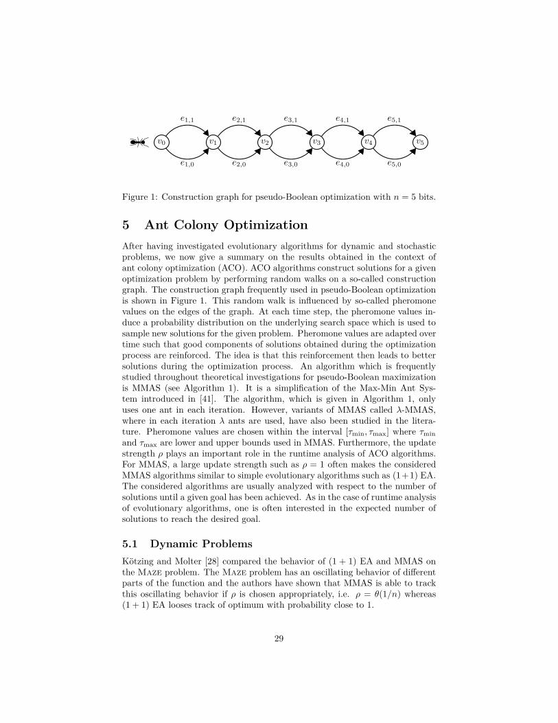
Figure 1: Construction graph for pseudo-Boolean optimization with n = 5 bits.

5 Ant Colony Optimization

After having investigated evolutionary algorithms for dynamic and stochasticproblems, we now give a summary on the results obtained in the context ofant colony optimization (ACO). ACO algorithms construct solutions for a givenoptimization problem by performing random walks on a so-called constructiongraph. The construction graph frequently used in pseudo-Boolean optimizationis shown in Figure 1. This random walk is influenced by so-called pheromonevalues on the edges of the graph. At each time step, the pheromone values in-duce a probability distribution on the underlying search space which is used tosample new solutions for the given problem. Pheromone values are adapted overtime such that good components of solutions obtained during the optimizationprocess are reinforced. The idea is that this reinforcement then leads to bettersolutions during the optimization process. An algorithm which is frequentlystudied throughout theoretical investigations for pseudo-Boolean maximizationis MMAS (see Algorithm 1). It is a simplification of the Max-Min Ant Sys-tem introduced in [41]. The algorithm, which is given in Algorithm 1, onlyuses one ant in each iteration. However, variants of MMAS called λ-MMAS,where in each iteration λ ants are used, have also been studied in the litera-ture. Pheromone values are chosen within the interval [τmin, τmax] where τmin

and τmax are lower and upper bounds used in MMAS. Furthermore, the updatestrength ρ plays an important role in the runtime analysis of ACO algorithms.For MMAS, a large update strength such as ρ = 1 often makes the consideredMMAS algorithms similar to simple evolutionary algorithms such as (1+1) EA.The considered algorithms are usually analyzed with respect to the number ofsolutions until a given goal has been achieved. As in the case of runtime analysisof evolutionary algorithms, one is often interested in the expected number ofsolutions to reach the desired goal.

5.1 Dynamic Problems

Kotzing and Molter [28] compared the behavior of (1 + 1) EA and MMAS onthe Maze problem. The Maze problem has an oscillating behavior of differentparts of the function and the authors have shown that MMAS is able to trackthis oscillating behavior if ρ is chosen appropriately, i.e. ρ = θ(1/n) whereas(1 + 1) EA looses track of optimum with probability close to 1.

29

Algorithm 1 MMAS

1: Set τ(u,v) = 1/2 for all (u, v) ∈ E.2: Construct a solution x∗.3: Update pheromones w.r.t. x∗.4: repeat forever

5: Construct a solution x.6: if f(x) ≥ f(x∗) then x∗ := x.7: Update pheromones w.r.t. x∗.

In the case of dynamic combinatorial optimization problems, dynamic single-source shortest paths problems have been investigated in [30]. Given a destina-tion node t ∈ V , the goal is to compute for any node v ∈ V \ t a shortest pathsfrom v to t. The set of these single-source shortest paths can be represented as atree with root t and the path from v to t in that tree gives a shortest path from vto t. The authors have investigated different types of dynamic changes for vari-ants of MMAS. They first investigated the MMAS and show that this algorithmcan effectively deal with one time changes and build on investigations in [42]for the static case. They show that the algorithm is able to recompute single-source shortest paths in an expected number of O(ℓ∗/τmin + ℓ ln(τmax/τmin)/ρ)iterations after a one change has happened. The parameter ℓ denotes the max-imum number of arcs in any shortest path to node t in the new graph andℓ∗ = minℓ, log n. The result shows that MMAS is able to track dynamicchanges if they are not too frequent. Furthermore, they present a lower boundof Ω(ℓ/τmin) in the case that ρ = 1 holds. Afterwards, periodic local and globalchanges are investigated. In the case of the investigated local changes, λ-MMASwith a small λ is able to track periodic local changes for a specific setting. Forglobal changes, a setting with oscillation between two simple weight functions isintroduced where an exponential number of ants would be required to make surethat an optimal solution is sampled with constant probability in each iteration.

5.2 Stochastic Problems

In stochastic environments, ACO algorithms have been analyzed for exemplarybenchmark functions and the stochastic shortest paths problem.

Thyssen and Sudholt [4] started the runtime analysis of ACO algorithmsin stochastic environments. They investigated the single-destination shortestpath (SDSP) problem where edge weights are subject to noise. For each edgee the noise model return a weight of (1 + η(e, p, t)) · w(e) instead of the exactreal weight w(e). This implies that the weight w(e) of each edge e is increasedaccording to the noise model. They considered a variant of MMAS for theshortest path problem introduced in [42]. They start by characterizing noisemodel for which the algorithm can discover shortest paths efficiently. In thegeneral setting, they examined the algorithms in terms of approximations. Theresults depends on how much non optimal paths differ at least from optimalones. More precisely, they show that if for each vertex v ∈ V and some α > 1 it

30

holds that every non-optimal path has length at least (1 + α ·E(η(optv))) · optv

then the algorithm finds an α-approximation in time proportional to α/(α− 1)and other standard ACO parameters such as pheromone bounds and pheromoneupdate strengths. Here optv denotes the value of a shortest paths from v tothe destination t and E(η(optv)) denotes the expected random noise on alledges of this path. Furthermore, for independent gamma-distributions alongthe edges, they have shown that the algorithm may need exponential time tofind a good approximation. Doerr et al. [7] have extended the investigationsfor the stochastic SDSP problem. They considered a slight variation of MMASfor the stochastic SDSP which always reevaluates the best so-far solution whena new solution for comparison is obtained. This allows the MMAS version toeasily obtain shortest paths in the stochastic setting.

Friedrich et al. [14] considered MMAS with a fitness proportional pheromoneupdate rule on linear pseudo-Boolean functions. They show that the algorithmscales gracefully with the noise, i.e. the runtime only depends linearly on thevariance of the Gaussian noise. In contrast to this many of the considerednoise settings are not solvable by simple evolutionary algorithms such as (1 +1) EA [11]. This points out a clear benefit of using ant colony optimization forstochastic problems.

6 Conclusions

Evolutionary algorithms have been extensively used to deal with dynamic andstochastic problems. We have given an overview on recent results regarding thetheoretical foundations of evolutionary algorithms for dynamic and stochasticproblems in the context of rigorous runtime analysis. Various results for dynamicproblems in the context of combinatorial optimization for problems such asmakespan scheduling and minimum vertex cover have been summarized andthe benefits of different approaches to deal with such dynamic problems havebeen pointed out. In the case of stochastic problems, the impact on the amountof noise and how population-based approaches are beneficial for coping withnoisy environments have been summarized.

While all these studies have greatly contributed to the understanding of thebasic working principles of evolutionary algorithms and ant colony optimizationin dynamic and stochastic environments, analyzing the behavior on complexproblems remains highly open. Furthermore, also uncertainties often changeover time and are therefore dynamic. Therefore, it would be very interestingto analyze the behavior of evolutionary algorithms for problems where uncer-tainties change over time. For future research, it would also be interesting toexamine environments that are both dynamic and stochastic as many real-worldproblems have both properties at the same time.

31

References

[1] Y. Akimoto, S. Astete-Morales, and O. Teytaud. Analysis of runtime ofoptimization algorithms for noisy functions over discrete codomains. The-oretical Computer Science, 605:42–50, 2015.

[2] S. Astete-Morales, M.-L. Cauwet, and O. Teytaud. Analysis of differenttypes of regret in continuous noisy optimization. In Proceedings of theGenetic and Evolutionary Computation Conference 2016, pages 205–212.ACM, 2016.

[3] S. Cathabard, P. K. Lehre, and X. Yao. Non-uniform mutation rates forproblems with unknown solution lengths. In H. Beyer and W. B. Lang-don, editors, Foundations of Genetic Algorithms, 11th International Work-shop, FOGA 2011, Schwarzenberg, Austria, January 5-8, 2011, Proceed-ings, pages 173–180. ACM, 2011.

[4] C. A. C. Coello, V. Cutello, K. Deb, S. Forrest, G. Nicosia, and M. Pavone,editors. Parallel Problem Solving from Nature - PPSN XII - 12th Inter-national Conference, Taormina, Italy, September 1-5, 2012, Proceedings,Part I, volume 7491 of Lecture Notes in Computer Science. Springer, 2012.

[5] B. Doerr, C. Doerr, and F. Ebel. From black-box complexity to designingnew genetic algorithms. Theor. Comput. Sci., 567(C):87–104, Feb. 2015.

[6] B. Doerr, C. Doerr, and T. Kotzing. Solving problems with unknownsolution length at (almost) no extra cost. In S. Silva and A. I. Esparcia-Alcazar, editors, Proceedings of the Genetic and Evolutionary ComputationConference, GECCO 2015, Madrid, Spain, July 11-15, 2015, pages 831–838. ACM, 2015.

[7] B. Doerr, A. Hota, and T. Kotzing. Ants easily solve stochastic shortestpath problems. In T. Soule and J. H. Moore, editors, Genetic and Evo-lutionary Computation Conference, GECCO ’12, Philadelphia, PA, USA,July 7-11, 2012, pages 17–24. ACM, 2012.

[8] B. Doerr, D. Johannsen, and C. Winzen. Multiplicative drift analysis.Algorithmica, 64(4):673–697, 2012.

[9] S. Droste. Analysis of the (1+1) EA for a dynamically changing ONEMAX-variant. In Evolutionary Computation, 2002. CEC ’02. Proceedings of the2002 Congress on, volume 1, pages 55–60, May 2002.

[10] S. Droste. Analysis of the (1+1) ea for a dynamically bitwise changingonemax. In Proceedings of the 2003 International Conference on Geneticand Evolutionary Computation: PartI, GECCO’03, pages 909–921, Berlin,Heidelberg, 2003. Springer-Verlag.

32

[11] S. Droste. Analysis of the (1+ 1) EA for a noisy OneMax. In Geneticand Evolutionary Computation–GECCO 2004, pages 1088–1099. Springer,2004.

[12] T. Friedrich, J. He, N. Hebbinghaus, F. Neumann, and C. Witt. Approx-imating covering problems by randomized search heuristics using multi-objective models. Evolutionary Computation, 18(4):617–633, 2010.

[13] T. Friedrich, T. Kotzing, M. S. Krejca, and A. M. Sutton. Graceful scal-ing on uniform versus steep-tailed noise. In International Conference onParallel Problem Solving from Nature, pages 761–770. Springer, 2016.

[14] T. Friedrich, T. Kotzing, M. S. Krejca, and A. M. Sutton. Robustness ofant colony optimization to noise. Evolutionary Computation, 24(2):237–254, 2016.

[15] T. Friedrich, T. Kotzing, G. Lagodzinski, F. Neumann, and M. Schirneck.Analysis of the (1+1) EA on subclasses of linear functions under uniformand linear constraints. In Proceedings of the 14th ACM/SIGEVO Confer-ence on Foundations of Genetic Algorithms, FOGA ’17, pages 45–54, NewYork, NY, USA, 2017. ACM.

[16] T. Friedrich, T. Kotzing, and A. M. Sutton. On the robustness of evolvingpopulations. In International Conference on Parallel Problem Solving fromNature, pages 771–781. Springer, 2016.

[17] T. Friedrich, T. Kotzing, M. S. Krejca, and A. M. Sutton. The bene-fit of recombination in noisy evolutionary search. In K. Elbassioni andK. Makino, editors, International Symposium of Algorithms and Compu-tation (ISAAC), pages 140–150, Berlin, Heidelberg, 2015. Springer BerlinHeidelberg.

[18] T. Friedrich, T. Kotzing, M. S. Krejca, and A. M. Sutton. The benefit ofrecombination in noisy evolutionary search. In Genetic and EvolutionaryComputation Conference (GECCO), pages 161–162, 2016.

[19] T. Friedrich, T. Kotzing, M. S. Krejca, and A. M. Sutton. Robustness ofant colony optimization to noise. Evolutionary Computation, 24(2):237–254, 2016.

[20] T. Friedrich, T. Kotzing, M. S. Krejca, and A. M. Sutton. The compactgenetic algorithm is efficient under extreme gaussian noise. IEEE Transac-tions on Evolutionary Computation, 21(3):477–490, 2017.

[21] T. Friedrich, T. Kotzing, and A. M. Sutton. On the robustness of evolvingpopulations. In Parallel Problem Solving From Nature (PPSN), pages 771–781, 2016.

[22] C. Gießen and T. Kotzing. Robustness of populations in stochastic envi-ronments. Algorithmica, 75(3):462–489, 2016.

33

[23] T. Jansen, P. S. Oliveto, and C. Zarges. Approximating vertex cover usingedge-based representations. In F. Neumann and K. A. D. Jong, editors,Foundations of Genetic Algorithms XII, FOGA ’13, Adelaide, SA, Aus-tralia, January 16-20, 2013, pages 87–96. ACM, 2013.

[24] T. Jansen and C. Zarges. Evolutionary algorithms and artificial immunesystems on a bi-stable dynamic optimisation problem. In Proceedings ofthe 2014 Annual Conference on Genetic and Evolutionary Computation,GECCO ’14, pages 975–982, New York, NY, USA, 2014. ACM.

[25] T. Jansen and C. Zarges. Analysis of randomised search heuristics fordynamic optimisation. Evolutionary Computation, 23(4):513 – 541, 2015.

[26] H. Kellerer, U. Pferschy, and D. Pisinger. Knapsack Problems. Springer-Verlag Berlin Heidelberg, 2004.

[27] T. Kotzing, A. Lissovoi, and C. Witt. (1+1) ea on generalized dynamiconemax. In Proceedings of the 2015 ACM Conference on Foundations ofGenetic Algorithms XIII, FOGA ’15, pages 40–51, New York, NY, USA,2015. ACM.

[28] T. Kotzing and H. Molter. ACO beats EA on a dynamic pseudo-booleanfunction. In Coello et al. [4], pages 113–122.

[29] S. Kratsch and F. Neumann. Fixed-parameter evolutionary algorithms andthe vertex cover problem. Algorithmica, 65(4):754–771, 2013.

[30] A. Lissovoi and C. Witt. Runtime analysis of ant colony optimization ondynamic shortest path problems. Theoretical Computer Science, 561:73 –85, 2015. Genetic and Evolutionary Computation.

[31] A. Lissovoi and C. Witt. Mmas versus population-based ea on a family ofdynamic fitness functions. Algorithmica, 75(3):554–576, Jul 2016.

[32] A. Lissovoi and C. Witt. Mmas versus population-based ea on a family ofdynamic fitness functions. Algorithmica, 75(3):554–576, Jul 2016.

[33] A. Lissovoi and C. Witt. A runtime analysis of parallel evolutionary algo-rithms in dynamic optimization. Algorithmica, 78(2):641–659, Jun 2017.

[34] F. Neumann and C. Witt. On the runtime of randomized local searchand simple evolutionary algorithms for dynamic makespan scheduling. InIJCAI, pages 3742–3748, 2015.

[35] P. S. Oliveto, J. He, and X. Yao. Analysis of the (1+1)-EA for findingapproximate solutions to vertex cover problems. IEEE Trans. EvolutionaryComputation, 13(5):1006–1029, 2009.

34

[36] M. Pourhassan, W. Gao, and F. Neumann. Maintaining 2-approximationsfor the dynamic vertex cover problem using evolutionary algorithms. InProceedings of the 2015 Annual Conference on Genetic and EvolutionaryComputation, GECCO ’15, pages 903–910, New York, NY, USA, 2015.ACM.

[37] M. Pourhassan, F. Shi, and F. Neumann. Parameterized analysis of multi-objective evolutionary algorithms and the weighted vertex cover problem.In Proceedings of the 14th International Conference of Parallel ProblemSolving from Nature – PPSN XIV, pages 729–739. Springer InternationalPublishing, 2016.

[38] A. Prugel-Bennett, J. Rowe, and J. Shapiro. Run-time analysis ofpopulation-based evolutionary algorithm in noisy environments. In Proceed-ings of the 2015 ACM Conference on Foundations of Genetic AlgorithmsXIII, FOGA ’15, pages 69–75, New York, NY, USA, 2015. ACM.

[39] F. Shi, M. Schirneck, T. Friedrich, T. Kotzing, and F. Neumann. Reop-timization times of evolutionary algorithms on linear functions under dy-namic uniform constraints. In Proceedings of the Genetic and EvolutionaryComputation Conference, GECCO ’17, pages 1407–1414, New York, NY,USA, 2017. ACM.

[40] F. Shi, M. Schirneck, T. Friedrich, T. Kotzing, and F. Neumann. Reopti-mization time analysis of evolutionary algorithms on linear functions underdynamic uniform constraints. Algorithmica, May 2018.

[41] T. Stutzle and H. H. Hoos. MAX-MIN ant system. Future GenerationComp. Syst., 16(8):889–914, 2000.

[42] D. Sudholt and C. Thyssen. Running time analysis of ant colony opti-mization for shortest path problems. J. Discrete Algorithms, 10:165–180,2012.

[43] Y. Zhou and J. He. A runtime analysis of evolutionary algorithms forconstrained optimization problems. IEEE Transactions on EvolutionaryComputation, 11(5):608–619, Oct 2007.

35