Analysis of Covariance - B W Griffin · (dependent variable), say .60, we will be able to attribute 36% of the within group variance on the dependent variable to variability on I.Q

7Analysis of Covariance

7.1 INTRODUCTION

In Chapter 4 we examined the effect of two or more independent variables (factors)in explaining variation on the dependent variable. We set up an experimental de-sign, and thus this method is called experimental control. In this chapter we con-sider explaining variation on the dependent variable by measuring the subjects onsome other variable(s), called covariates, that are correlated with the dependentvariable. Recall that the square of a correlation can be interpreted as “proportion ofvariance accounted for.” Thus, if we find that I.Q. is correlated with achievement

285

CONTENTS7.1 Introduction7.2 Purposes of Covariance7.3 Adjustment of Posttest Means7.4 Reduction of Error Variance7.5 Choice of Covariates7.6 Numerical Example7.7 Assumptions in Analysis of Covariance7.8 Use of ANCOVA with Intact Groups7.9 Computer Example for ANCOVA7.10 Alternative Analyses7.11 An Alternative to the Johnson–Neyman Technique7.12 Use of Several Covariates7.13 Computer Example with Two Covariates7.14 Summary

(dependent variable), say .60, we will be able to attribute 36% of the within groupvariance on the dependent variable to variability on I.Q. In analysis of covariance(ANCOVA), this part of the variance is removed from the error term, and yields amore powerful test. This method of explaining variation is called statistical con-trol. We now consider an example to illustrate how ANCOVA can be very useful inan experimental study in which the subjects have been randomly assigned togroups.

Example

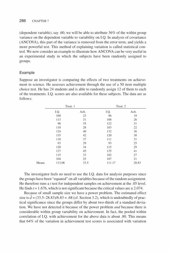
Suppose an investigator is comparing the effects of two treatments on achieve-ment in science. He assesses achievement through the use of a 50 item multiplechoice test. He has 24 students and is able to randomly assign 12 of them to eachof the treatments. I.Q. scores are also available for these subjects. The data are asfollows:

The investigator feels no need to use the I.Q. data for analysis purposes sincethe groups have been “equated” on all variables because of the random assignment.He therefore runs a t test for independent samples on achievement at the .05 level.He finds t = 1.676, which is not significant because the critical values are ± 2.074.

Because of small sample size we have a power problem. The estimated effectsize is �d = (33.5–28.83)/6.83 = .68 (cf. Section 3.2), which is undoubtedly of prac-tical significance since the groups differ by about two-thirds of a standard devia-tion. We have not detected it because of the power problem and because there isconsiderable within group variability on achievement. In fact, the pooled withincorrelation of I.Q. with achievement for the above data is about .80. This meansthat 64% of the variation in achievement test scores is associated with variation

286 CHAPTER 7

Treat. 1 Treat. 2

I.Q. Ach. I.Q. Ach.100 23 96 19113 31 108 2698 35 122 31

110 28 103 22124 40 132 36135 42 120 38118 37 111 3193 29 93 25

120 34 115 29127 45 125 41115 33 102 27104 25 107 21

Means 113.08 33.5 111.17 28.83

(individual differences) on I.Q. An analysis of covariance removes that portionfrom the error term and yields a t value significant at the .05 level (t = 2.25).Actually it comes out as an F statistic, so you need to take the square root. Recallthat F = t2 for two groups. After reading this chapter, the reader will be able to ver-ify the above t value by running the ANCOVA on SAS or SPSS.

The above example showed that analysis of covariance is very useful in creatinga more powerful test in an experimental study. ANCOVA is also used to reducebias when comparing intact or self-selected groups, such as males and females,Head Start and non-Head Start. A classical use is adjusting posttest means on thedependent variable for any initial differences that may have been present on a pre-test. Another typical use is in teaching methods studies that use intact classrooms.If the average I.Q.’s for the classrooms differ by 10 points, then an adjustment ofthe posttest achievement is done. Although the use of analysis of covariance in thiscontext may seem reasonable, it is quite controversial, which we discuss in detailin Section 7.8.

The first 10 sections of this chapter cover the basics for ANCOVA with onecovariate. We discuss the purposes of covariance, the underlying concepts, the as-sumptions, interpretation of results, the relationship of ANOVA and ANCOVA,and the running of ANCOVA on SAS and SPSS. The last five sections are more ad-vanced, especially the section on the Johnson–Neyman technique, and may beskipped without loss of continuity. Much has been written about analysis ofcovariance, and the reader should at least be aware of two classic review articles byCochran (1957) and Elashoff (1969), and a very comprehensive and thoroughbook on covariance and alternatives by Huitema (1980).

7.2 PURPOSES OF COVARIANCE

Analysis of covariance is related to the following two basic objectives in experi-mental design:

1. Elimination of systematic bias.2. Reduction of within group or error variance.

Systematic bias means that the groups differ systematically on some key vari-able(s) that are related to performance on the dependent variable. If the groups in-volve treatments, then a significant difference on a posttest at the end of treatmentswill be confounded (mixed in with) with initial differences on a key variable. Itwould not be clear whether the treatments were making the difference, or whetherinitial differences simply transferred to posttest means. A simple example is ateaching methods study with initial differences between groups on I.Q. Supposetwo methods of teaching algebra are compared (same teacher for both methods)

ANALYSIS OF COVARIANCE 287

with two classrooms in the same school. The following summary data, means forthe groups, are available:

If the t test for independent samples on the posttest is significant, then it isn’tclear whether it was method 1 that made the difference, or the fact that the childrenin that class were “brighter” to begin with, and thus would be expected to achievehigher scores.

As another example, suppose we are comparing the effect of four stress situa-tions on blood pressure (the dependent variable). It is found that situation 3 is sig-nificantly more stressful than the other three situations. However, we note that theblood pressure of the subjects in group 3 under minimal stress is greater than forthe subjects in the other groups. Then, it isn’t clear that situation 3 is necessarilymost stressful. We need to determine whether the blood pressure for group 3 wouldstill be higher if the posttest means for all 4 groups were “adjusted” in some way toaccount for initial differences in blood pressure. We see later that the posttestmeans are adjusted in a linear fashion to what they would be if all groups startedout equally on the covariate, that is, at the grand mean.

The best way of dealing with systematic bias is to randomly assign subjects togroups. Then we can be confident, within sampling error, that the groups don’t dif-fer systematically on any variables. Of course, in many studies random assign-ment is not possible, so we look for ways of at least partially equating groups. Oneway of partially controlling for initial differences is to match on key variables. Ofcourse, then we can only be sure the groups are equivalent on those matched vari-ables. Analysis of covariance is a statistical way of controlling on key variables.Once again, as with matching, ANCOVA can only reduce bias, and not eliminateit.

Why is reduction of error variance, the second purpose of analysis ofcovariance, important? Recall from Chapter 2 on one way ANOVA that the Fstatistic was F = MSh/MSw, where MSW was the estimate of error. If we can makeMSW smaller, then F will be larger and we will obtain a more sensitive or power-ful test. And from Chapter 3 on power, remember that power is generally poor insmall or medium sample size studies. Thus the use of perhaps 2 or 3 covariatesin such studies should definitely be considered. The use of covariates that haverelatively low correlations with each other are particularly helpful because eachcovariate removes a somewhat different part of the error variance from the de-pendent variable.

Analysis of covariance is a statistical way of reducing error variance. There areseveral other ways of reducing error variance. One way is through sample selec-

288 CHAPTER 7

Method 1 Method 2

I.Q. 120.2 105.8Posttest 73.4 67.5

tion; subjects who are more homogeneous vary less on the dependent measure.Another way, discussed in Chapter 4 on factorial designs, was to block on a vari-able, or consider it as another factor in the design.

7.3 ADJUSTMENT OF POSTTEST MEANS

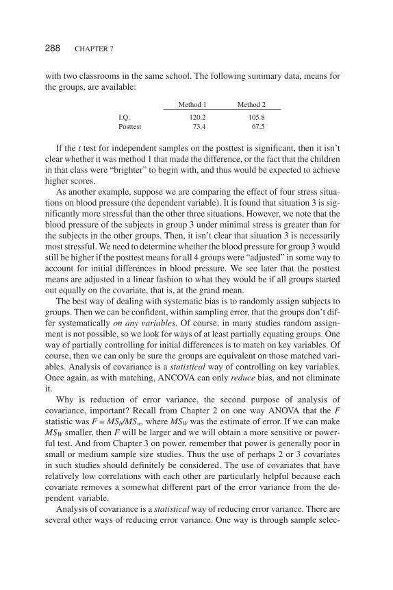
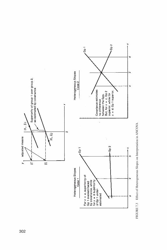
As mentioned earlier, analysis of covariance adjusts the posttest means to whatthey would be if all groups started out equally on the covariate; at the grand mean.In this section we derive the general equation for linearly adjusting the posttestmeans for one covariate. Before we do that, however, it is important to discuss oneof the assumptions underlying the analysis of covariance. That assumption for onecovariate requires equal population regression slopes for all groups. Consider athree group situation, with 15 subjects per group. Suppose that the scatterplots forthe 3 groups looked as given below.

Recall from beginning statistics that the x and y scores for each subject deter-mine a point in the plane. Requiring that the slopes be equal is equivalent to sayingthat the nature of the linear relationship is the same for all groups, or that the rate ofchange in y as a function of x is the same for all groups. For the above scatterplotsthe slopes are different, with the slope being the largest for group 2 and smallest forgroup 3. But the issue is whether the population slopes are different, and whetherthe sample slopes differ sufficiently to conclude that the population values are dif-ferent. With small sample sizes as in the above scatterplots, it is dangerous to relyon visual inspection to determine whether the population values are equal, becauseof considerable sampling error. Fortunately there is a statistic for this, and later weindicate how to obtain it on SPSS and SAS. In deriving the equation for the ad-justed means we are going to assume the slopes are equal. What if the slopes arenot equal? Then ANCOVA is not appropriate, and we indicate alternatives later onin the chapter.


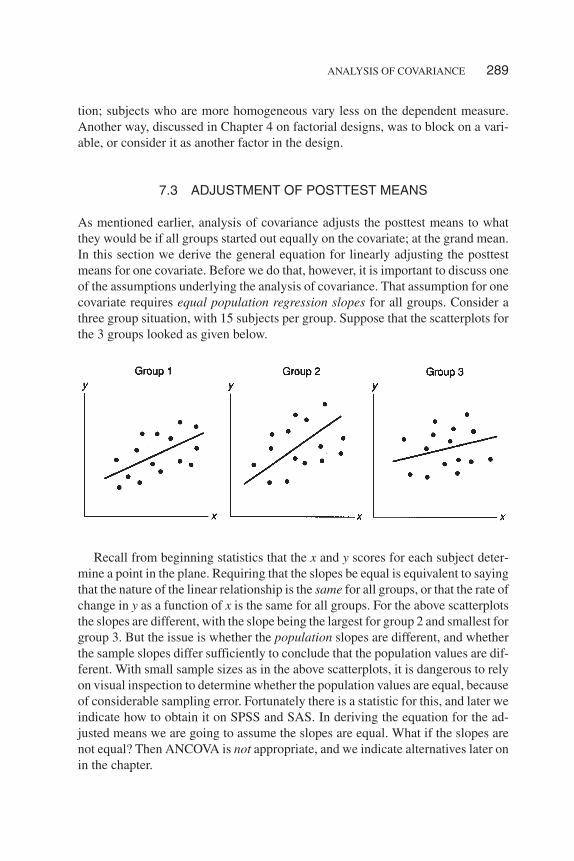
The details of obtaining the adjusted mean for the ith group (i.e., any group) aregiven in Figure 7.1. The general equation follows from the definition for the slopeof a straight line and some basic algebra.

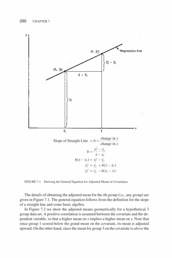
In Figure 7.2 we show the adjusted means geometrically for a hypothetical 3group data set. A positive correlation is assumed between the covariate and the de-pendent variable, so that a higher mean on x implies a higher mean on y. Note thatsince group 1 scored below the grand mean on the covariate, its mean is adjustedupward. On the other hand, since the mean for group 3 on the covariate is above the

290 CHAPTER 7

FIGURE 7.1 Deriving the General Equation for Adjusted Means in Covariance

*

*

*

*

change inSlope of Straight Line

change in

( )

( )

( )

i i

i

i i i

i ii

i ii

yb

xy y

bx x

b x x y y

y y b x x

y y b x x

� �

�

�

�

� � �

� � �

� � �

grand mean, covariance estimates that it would have scored lower on y if its meanon the covariate was lower (at grand mean), and therefore the mean for group 3 isadjusted downward.


Group 1 Group 2 Group 3

xi 32 34 42yi 70 65 62yi

* 72 66 59

A common slope = .5 is being assumed here.

� The arrows on the regression lines indicate that the means are adjusted linearly upward or down-ward to what they would be if the groups had started out at the grand mean on the covariate.

FIGURE 7.2 Means and Adjusted Means for Hypothetical Three Group Data Set

* * *1 2 370 .5(32 36), 65 .5(34 36), 62 .5(42 36)y y y� � � � � � � � �

7.4 REDUCTION OF ERROR VARIANCE

It is relatively simple to derive the approximate error term for covariance. Denotethe correlation between the covariate (x) and the dependent variable (y) by rxy. Thesquare of a correlation can be interpreted as “proportion of variance accountedfor.” The within group variance for ANOVA is MSW. Thus, the part of the withingroup variance on y that is accounted for by the covariate is rxy2 MSW. The withinvariability left, after the portion due to the covariate is removed, is

and this becomes our new error term for the analysis of covariance, which we de-note by MSW*. Technically, there is an additional part to the adjusted error term:

where fe is the error degrees of freedom. However, the effect of this additional fac-tor is slight as long as N > 50.

To show how much of a difference a covariate can make in increasing the sensi-tivity of an experiment, we consider a hypothetical study. An investigator runs aone-way ANOVA (3 groups and 20 subjects per group), and obtains F = 200/100 =2, which is not significant, because the critical value at .05 is 3.18. He pretested thesubjects, but didn’t use the pretest as a covariate (even though the correlation be-tween covariate and posttest was .71) because the groups didn’t differ significantlyon the pretest. This is a common mistake made by some researchers who are un-aware of the other purpose of covariance, that of reducing error variance. The anal-ysis is redone by another investigator using ANCOVA. Using the equation we justderived she finds

Thus, the error term for the ANCOVA is only half as large as the error term forANOVA. It is also necessary to obtain a new MSb* for ANCOVA, call it MSb*. InSection 7.6 we show how to calculate MSb*. Let us assume here that the investiga-tor obtains the following F ratio for the covariance analysis:

This is significant at the .05 level. Therefore, the use of covariance can make thedifference between finding and not finding significance. Finally, we wish to notethat MSb* can be smaller or larger than MSb although in a randomized study the ex-pected values of the two are equal.

292 CHAPTER 7

2 2(1 ) (1)w w xy w xyMS MS r MS r� � �

2* (1 )[1 1/( 2)]w w xy eMS MS r f� � � �

* 2100[1 (.71) ] 50wMS � � �

* 190 / 50 3.8F � �

7.5 CHOICE OF COVARIATES

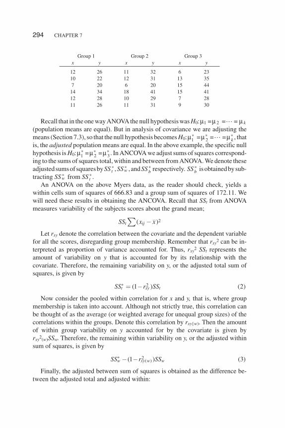
In general, any variables that theoretically should correlate with the dependentvariable, or variables that have been shown to correlate on similar types of sub-jects, should be considered as possible covariates. The ideal is to choose ascovariates variables that of course are significantly correlated with the dependentvariable and have low correlations among themselves. If two covariates are highlycorrelated (say .80), then they are removing much of the same error variance fromy; x2 will not have much incremental validity. On the other hand, if two covariates(x1 and x2) have a low correlation (say .20), then they are removing relatively dis-tinct pieces of the error variance from y, and we will obtain a much greater total er-ror reduction. This is illustrated graphically below using Venn diagrams, where thecircle represents error variance on y.

The shaded portion in each case represents the incremental validity of x2, that is,the part of error variance on y it removes that x1 did not.

Huitema (1980, p. 161) has recommended limiting the number of covariates tothe extent that the ratio

where C is the number of covariates, J is the number of groups, and N is total sam-ple size. Thus, if we had a four group problem with a total of 80 subjects, then (C +3)/80 < .10 or C < 5. Less than 5 covariate should be used. If the above ratio is >.10, then the adjusted means are likely to be unstable.

7.6 NUMERICAL EXAMPLE

We now consider an example to illustrate how to calculate an ANCOVA and tomake clear what the null hypothesis is that is being tested. We use the following 3group data set from Myers (1979, p. 417), where x indicates the covariate:


[ ( 1)].10

C J

N

� �

�

Recall that in the one way ANOVA the null hypothesis was H0:µ1 =µ 2 =� = µ k

(population means are equal). But in analysis of covariance we are adjusting themeans (Section 7.3), so that the null hypothesis becomes H0:µ1

* =µ 2* =� =µ k

* , thatis, the adjusted population means are equal. In the above example, the specific nullhypothesis is H0:µ1

* =µ 2* =µ 3

* . In ANCOVA we adjust sums of squares correspond-ing to the sums of squares total, within and between from ANOVA. We denote theseadjustedsumsofsquaresbySSt

* ,SSw* , andSSb* respectively. SSb

* isobtainedbysub-tracting SSw* from SSt

* .An ANOVA on the above Myers data, as the reader should check, yields a

within cells sum of squares of 666.83 and a group sum of squares of 172.11. Wewill need these results in obtaining the ANCOVA. Recall that SSt from ANOVAmeasures variability of the subjects scores about the grand mean;

Let rxy denote the correlation between the covariate and the dependent variablefor all the scores, disregarding group membership. Remember that rxy2 can be in-terpreted as proportion of variance accounted for. Thus, rxy2 SSt represents theamount of variability on y that is accounted for by its relationship with thecovariate. Therefore, the remaining variability on y, or the adjusted total sum ofsquares, is given by

Now consider the pooled within correlation for x and y, that is, where groupmembership is taken into account. Although not strictly true, this correlation canbe thought of as the average (or weighted average for unequal group sizes) of thecorrelations within the groups. Denote this correlation by rxy{w). Then the amountof within group variability on y accounted for by the covariate is given byrxy2(w)SSw. Therefore, the remaining within variability on y, or the adjusted withinsum of squares, is given by

Finally, the adjusted between sum of squares is obtained as the difference be-tween the adjusted total and adjusted within:

294 CHAPTER 7

2( )t ijSS x x��

2* (1 ) (2)t xy tSS r SS� �

2* ( )(1 ) (3)w xy w wSS r SS� �

Group 1 Group 2 Group 3x y x y x y

12 26 11 32 6 2310 22 12 31 13 357 20 6 20 15 4414 34 18 41 15 4112 28 10 29 7 2811 26 11 31 9 30

The F ratio for analysis of covariance is then given by

where C is the number of covariates. Note that one degree of freedom for error islost for each covariate used.

This method of computing the ANCOVA is conceptually fairly simple, and im-portantly shows its direct linkage with the results from an ANOVA on the samedata. The SAS GLM control lines for running the ANCOVA are presented in Table7.1, along with selected printout. The total correlation is .85286 and the withingroup correlations are gp 1: .9316, gp 2: .9799, and gp 3: .9708. Using these re-sults, the F ratio for the ANCOVA is easily obtained. First, from Equation 2 wehave that


* * * (4)t wbSS SS SS� �

* * * * *( /( 1)) / /( ) / (5)w wb bF SS k SS N K C MS MS� � � � �

* 2(1 (.85286) )838.94 228.72tSS � �

Placeholder for T0701 from p. 315 of previous edition

TABLE 7.1SAS GLM Control Lines and Selected Printout for ANCOVA on MyersData and SPSS Windows 12.0 Interactive Plots and Regression Lines

Now, using the average of the within correlations as a rough estimate of thepooled within correlation, we find that r = (.9316 + .9799 + .9708)/3 = .9608 (theactual pooled correlation is .965). Now, using Equation 3 we find the adjustedwithin sum of squares:

Therefore, the adjusted between sum of squares is:

296 CHAPTER 7

* 2(1 (.965) )(666.83) 45.86wSS � � �

Place holder for T0701-b from p. 316 of previous edition.

TABLE 7.1(Continued)

and the F ratio for the analysis of covariance is

ANCOVA as a Special Case of Multiple Regression

Since analysis of covariance involves both analysis of variance and regressionanalysis, we can do an ANCOVA using multiple regression. Recall that in the lastchapter on regression analysis we showed that ANOVA was a special case of re-gression analysis. We dummy coded group membership and used these dummyvariables to predict the dependent variable.

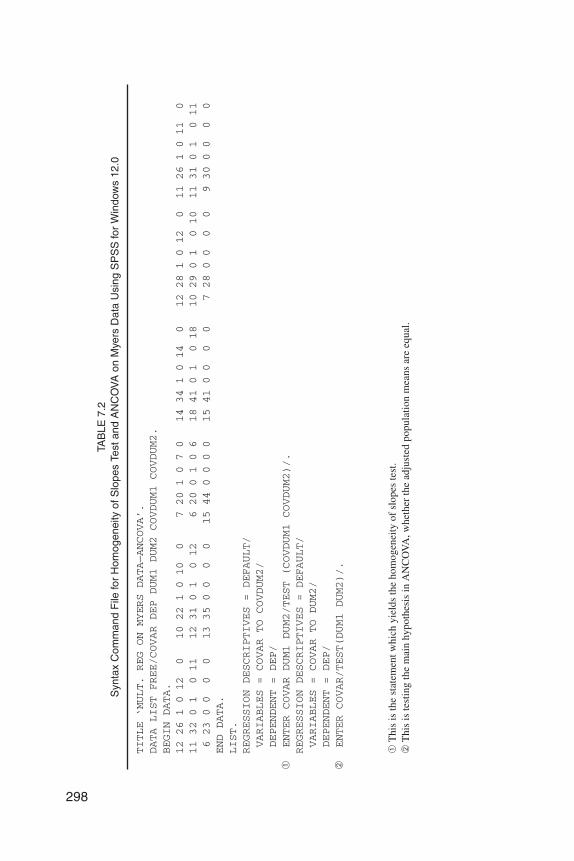
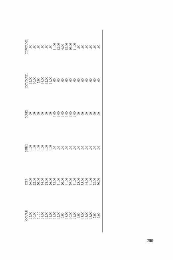
We will illustrate how an ANCOVA can be done using multiple regression withthe Myers data. First, we shall check the homogeneity of regression slopes as-sumption. For a one way design, as Myers and Well (1991, p. 567) point out, “Per-forming an ANCOVA on a design that has a single factor A can now be seen as de-termining whether A has effects over and above those of the covariate x. “Thus, weforce the covariate in and then determine whether group membership has an effectabove and beyond the covariate. Since we have 3 groups here, we will need twodummy variables to code group membership (we denote them by DUM1, DUM2).Recall that a violation of the slopes assumption meant there was a group bycovariate interaction. Thus, we set up an interaction effect and test it for signifi-cance. We create the group by covariate interaction effects by multiplying (we de-note them by COVDUM1 and COVDUM2) and then test these for significance.The complete control lines for testing homogeneity of slopes and doing theANCOVA are presented in Table 7.2.

Selected printout from SPSS for Windows 12.0 is presented in Table 7.3. Notethat the assumption of equal regression slopes is tenable (F = .354), and that theANCOVA is significant (F = 27.886).

7.7 ASSUMPTIONS IN ANALYSIS OF COVARIANCE

Analysis of covariance rests on the same assumptions as the analysis of varianceplus three additional assumptions regarding the regression part of the covarianceanalysis. ANCOVA also assumes

1. A linear relationship between the dependent variable and the covariate(s).


* (182.86 / 2) / 45.86 /(18 3 1) 27.87F � � � �

* 228.72 45.86 182.86bSS � � �

298

TAB

LE7.

2S

ynta

xC

omm

and

File

for

Hom

ogen

eity

ofS

lope

sTe

stan

dA

NC

OV

Aon

Mye

rsD

ata

Usi

ngS

PS

Sfo

rW

indo

ws

12.0

TITLE‘MULT.REGONMYERSDATA—ANCOVA’.

DATALISTFREE/COVARDEPDUM1DUM2COVDUM1COVDUM2.

BEGINDATA.

12261012

010221010

07201070

14341014

012281012

011261011

0113201

011

123101

012

6200106

184101

018

102901

010

113101

011

62300

00

133500

00

15440000

154100

00

72800

00

93000

00

ENDDATA.

LIST.

REGRESSIONDESCRIPTIVES=DEFAULT/

VARIABLES=COVARTOCOVDUM2/

DEPENDENT=DEP/

�ENTERCOVARDUM1DUM2/TEST(COVDUM1COVDUM2)/.

REGRESSIONDESCRIPTIVES=DEFAULT/

VARIABLES=COVARTODUM2/

DEPENDENT=DEP/

�ENTERCOVAR/TEST(DUM1DUM2)/.

�T

his

isth

est

atem

entw

hich

yiel

dsth

eho

mog

enei

tyof

slop

este

st.

�T

his

iste

stin

gth

em

ain

hypo

thes

isin

AN

CO

VA

,whe

ther

the

adju

sted

popu

latio

nm

eans

are

equa

l.

299

COVAR

DEP

DUM1

DUM2

COVDUM1

COVDUM2

12.0

026

.00

1.00

.00

12.0

0.0

010

.00

22.0

01.

00.0

010

.00

.00

7.00

20.0

01.

00.0

07.

00.0

014

.00

34.0

01.

00.0

014

.00

.00

12.0

028

.00

1.00

.00

12.0

0.0

011

.00

26.0

01.

00.0

011

.00

.00

11.0

032

.00

.00

1.00

.00

11.0

012

.00

31.0

0.0

01.

00.0

012

.00

6.00

20.0

0.0

01.

00.0

06.

0018

.00

41.0

0.0

01.

00.0

018

.00

10.0

029

.00

.00

1.00

.00

10.0

011

.00

31.0

0.0

01.

00.0

011

.00

6.00

23.0

0.0

0.0

0.0

0.0

013

.00

35.0

0.0

0.0

0.0

0.0

015

.00

44.0

0.0

0.0

0.0

0.0

015

.00

41.0

0.0

0.0

0.0

0.0

07.

0028

.00

.00

.00

.00

.00

9.00

30.0

0.0

0.0

0.0

0.0

0

2. Homogeneity of the regression slopes (for one covariate); parallelism ofthe regression planes for two covariates and for more than 2 covariates ho-mogeneity of the regression hyperplanes.

3. The covariate is measured without error.

Since covariance rests on the same assumptions as ANOVA, any violations thatare serious in ANOVA (like dependent observations) are also serious in ANCOVA.Violation of all 3 of the above regression assumptions can also be serious. For ex-ample, if the relationship between the covariate and the dependent variable iscurvilinear, then the adjustment of the means will be improper.

There is always measurement error for the variables that are typically used ascovariates in social science research. In randomized designs this reduces the powerof the ANCOVA, but treatment effects are not biased. For non-randomized designsthe treatment effects can be seriously biased.

A violation of the homogeneity of regression slopes can also yield quite mis-leading results. To illustrate this, we present in Figure 7.3 the situation where theassumption is met and two situations where the slopes are unequal. Notice thatwith equal slopes the estimated superiority of group 1 at the grand mean is a totallyaccurate estimate of group 1’s superiority for all levels of the covariate, since thelines are parallel. For Case 1 of unequal slopes there is a covariate by treatment in-teraction. That is, how much better group 1 is depends on which value of thecovariate we specify. This is analogous to the concept of interaction in a factorialdesign. For Case 2 of heterogeneous slopes the use of covariance would be totallymisleading. Covariance estimates no difference between the groups, while for x =c, group 2 is quite superior, and for x = d, group 1 is quite superior. Later in thechapter we show how to test the assumption of equal slopes on SPSS and on SAS.

Therefore, in examining printout from the statistical packages it is impor-tant to first make two checks to determine whether analysis of covariance isappropriate:

1. Check to see whether there is a linear relationship between the de-pendent variable and the covariate.

2. Check to determine whether the homogeneity of the regression slopesis tenable.

If the above assumptions are met, then there is not any debate about the appro-priateness of ANCOVA in randomized studies in which the subjects have been ran-domly assigned to groups. For intact groups, there is a debate, and we discuss thatin the next section.

If either of the above assumptions is not satisfied, then covariance is not ap-propriate. In particular, if (2) is not met, then one should consider using the

300 CHAPTER 7

301

TABLE 7.3Selected Printout From SPSS for Windows 12.0 for ANCOVA on Myers

Data Using Multiple Regression

� This is the test for a significant regression on y on the covariate.� This is the test for homogeneity of the regression slopes.� This is the main test in covariance; whether the adjusted population means are equal.

302

FIG

UR

E7.

3E

ffec

tof

Het

erog

eneo

usSl

opes

onIn

terp

reta

tion

inA

NC

OV

A

Johnson–Neyman (1936) technique. For extended discussion on the John-son–Neyman technique see Rogosa (1977, 1980).

7.8 USE OF ANCOVA WITH INTACT GROUPS

It should be noted that some researchers (Anderson, 1963; Lord, 1969) have ar-gued strongly against using analysis of covariance with intact groups. Althoughwe do not take this position, it is important that the reader be aware of the severallimitations and/or possible dangers when using ANCOVA with intact groups.First, even the use of several covariates will not equate intact groups, and oneshould never be deluded into thinking it can. The groups may still differ on someunknown important variable(s). Also, note that equating groups on one variablemay result in accentuating their differences on other variables.

Second, recall that ANCOVA adjusts the posttest means to what they would beif all the groups had started out equal on the covariate(s). You then need to considerwhether groups that are equal on the covariate would ever exist in the real world.Elashoff (1969) gives the following example. Teaching methods A and B are beingcompared. The class using A is composed of high ability students, whereas theclass using B is composed of low ability students. A covariance analysis can bedone on the posttest achievement scores holding ability constant, as if A and B hadbeen used on classes of equal and average ability. But, as Elashoff notes, “It maymake no sense to think about comparing methods A and B for students of averageability, perhaps each has been designed specifically for the ability level it was usedwith, or neither method will, in the future, be used for students of average ability”(p. 387).

Third, the assumptions of linearity and homogeneity of regression slopes needto be satisfied for ANCOVA to be appropriate.

A fourth issue that can confound the interpretation of results is differentialgrowth of subjects in intact or self selected groups on some dependent variable. Ifthe natural growth is much greater in one group (treatment) than for the controlgroup and covariance finds a significance difference, after adjusting for any pretestdifferences, then it isn’t clear whether the difference is due to treatment, differen-tial growth, or part of each. Bryk and Weisberg (1977) discuss this issue in detailand propose an alternative approach for such growth models.

A fifth problem is that of measurement error. Of course this same problem ispresent in randomized studies. But there the effect is merely to attenuate power. Innon-randomized studies measurement error can seriously bias the treatment effect.Reichardt (1979), in an extended discussion on measurement error in ANCOVA,states,


Measurement error in the pretest can therefore produce spurious treatment effectswhen none exist. But it can also result in a finding of no intercept difference when atrue treatment effect exists, or it can produce an estimate of the treatment effectwhich is in the opposite direction of the true effect. (p. 164)

It is no wonder then that Pedhadzur (1982, p. 524), in discussing the effect of mea-surement error when comparing intact groups, says,

The purpose of the discussion here was only to alert you to the problem in the hopethat you will reach two obvious conclusions: (1) that efforts should be directed toconstruct measures of the covariates that have very high reliabilities and (2) that ig-noring the problem, as is unfortunately done in most applications of ANCOVA, willnot make it disappear. (p. 524)

Porter (1967) has developed a procedure to correct ANCOVA for measurementerror, and an example illustrating that procedure is given in Huitema (1980, pp.315–316). This is beyond the scope of the present text.

Given all of the above problems, the reader may well wonder whether weshould abandon the use of covariance when comparing intact groups. But otherstatistical methods for analyzing this kind of data (such as matched samples, gainscore ANOVA) suffer from many of the same problems, such as seriously biasedtreatment effects. The fact is that inferring cause-effect from intact groups istreacherous, regardless of the type of statistical analysis. Therefore, the task is todo the best we can and exercise considerable caution, or as Pedhazur (1982) put it:“But the conduct of such research, indeed all scientific research, requires soundtheoretical thinking, constant vigilance, and a thorough understanding of the po-tential and limitations of the methods being used” (p. 525).

7.9 COMPUTER EXAMPLE FOR ANCOVA

To illustrate how to run an ANCOVA, while at the same time checking the criticalassumptions of linearity and homogeneity of slopes, we consider part of a SesameStreet data set from Glasnapp and Poggio (1985), who present data on many vari-ables, including 12 background variables and 8 achievement variables for 240 sub-jects. Sesame Street was developed as a television series aimed mainly at teachingpreschool skills to 3- to 5-year-old children. Data was collected at 5 different siteson many achievement variables both before (pretest) and after (posttest) viewingof the series. We consider here only the achievement variable of knowledge ofnumbers. The maximum possible score is 54 and the content of the items includedrecognizing numbers, naming numbers, counting, addition, and subtraction. Weuse ANCOVA to determine whether the posttest knowledge of numbers for the

304 CHAPTER 7

children at the first 3 sites differed after adjustments are made for any pretest dif-ferences.

In Table 7.4 we give the complete control lines for running the ANCOVA onSPSS MANOVA. Table 7.5 gives selected annotated output from that run. We indi-cate which of the F tests are checking the assumptions of linearity and homogene-ity of slopes, and which F addresses the main question in covariance (whether theadjusted population means are equal).

7.10 ALTERNATIVE ANALYSES

When comparing two or more groups with pretest and posttest data, the followingother modes of analysis have been used by many researchers:

1. An ANOVA is done on the difference or gain scores (posttest—pretest).2. A two way repeated measures (this is covered in Chapter 5) ANOVA is

done. This is also called a one between (the grouping variable) and onewithin (pretest-posttest part) factor ANOVA.


TABLE 7.4SPSS MANOVA Control Lines for Analysis of Covariance on Sesame

Street Data

TITLE ‘ANALYSIS OF COVARIANCE ON SESAME DATA’.DATA LIST FREE/SITE PRENUMB POSTNUMB.BEGIN DATA.

DATA (ON CD)END DATA.MANOVA PRENUMB POSTNUMB BY SITE(1,3) /

� ANALYSIS POSTNUMB WITH PRENUMB /� PRINT = PMEANS /

DESIGN /� ANALYSIS = POSTNUMB /

DESIGN = PRENUMB,SITE,PRENUMB BY SITE /� ANALYSIS = PRENUMB/.

� The covariate(s) follow the keyword WITH.� This PRINT subcommand is needed to obtain the adjusted means, which is what we are testing

for significance.� This ANALYSIS subcommand and the following DESIGN subcommand are needed to test the

homogeneity of the regression slopes assumption.� This ANALYSIS subcommand is used to test whether the sites differed significantly on the pre-

test.

306

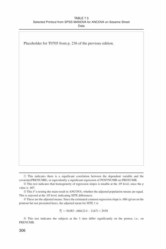
Placeholder for T0705 from p. 236 of the previous edition.

TABLE 7.5Selected Printout from SPSS MANOVA for ANCOVA on Sesame Street

Data

� This indicates there is a significant correlation between the dependent variable and thecovariate(PRENUMB), or equivalently a significant regression of POSTNUMB on PRENUMB.

� This test indicates that homogeneity of regression slopes is tenable at the .05 level, since the pvalue is .607.

� This F is testing the main result in ANCOVA; whether the adjusted population means are equal.This is rejected at the .05 level, indicating SITE differences.

� These are the adjusted means. Since the estimated common regression slope is .686 (given on theprintout but not presented here), the adjusted mean for SITE 1 is

y1 30 083 686 22 4 2167 2958* . . ( . . ) .� � � �

� This test indicates the subjects at the 3 sites differ significantly on the pretest, i.e., onPRENUMB.

Huck and McLean (1975) and Jennings (1988) have compared the above twomodes of analysis along with the use of ANCOVA for the pretest-posttest controlgroup design, and conclude that ANCOVA is the preferred method of analysis.Several comments from the Huck and McLean article are worth mentioning. First,they note that with the repeated measures approach it is the interaction F that is in-dicating whether the treatments had a differential effect, and not the treatmentmain effect. We consider two patterns of means below to illustrate.

In situation 1 the treatment main effect would probably be significant, becausethere is a difference of 10 in the row means. However, the difference of 10 on theposttest just transferred from an initial difference of 10 on the pretest. There is nota differential change in the treatment and control groups here. On the other hand, insituation 2 even though the treatment group scored higher on the pretest, it in-creased 15 points from pre to post while the control group increased just 8 points.That is, there was a differential change in performance in the two groups. But, re-call from Chapter 4 that one way of thinking of an interaction effect is as a “differ-ence in the differences.” This is exactly what we have in situation 2, hence a signifi-cant interaction effect.

Second, Huck and McLean (1975) note that the interaction F from the repeatedmeasures ANOVA is identical to the F ratio one would obtain from an ANOVA onthe gain (difference) scores. Finally, whenever the regression coefficient is notequal to 1 (generally the case), the error term for ANCOVA will be smaller than forthe gain score analysis and hence the ANCOVA will be a more sensitive or power-ful analysis.

Although not discussed in the Huck and McLean paper, we would like to add ameasurement caution against the use of gain scores. It is a fairly well known mea-surement fact that the reliability of gain (difference) scores is generally not good.To be more specific, as the correlation between the pretest and posttest scores ap-proaches the reliability of the test, the reliability of the difference scores goes to 0.The following table from Thorndike and Hagen (1977) quantifies things:


Situation 1 Situation 2Pretest Posttest Pretest Posttest

Treat. 70 80 Treat 65 80Control 60 70 Control 60 68

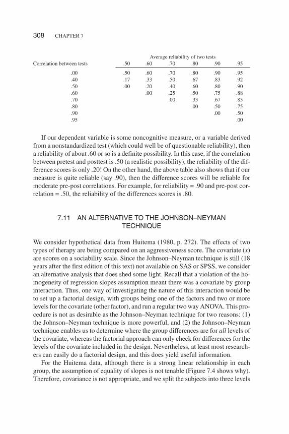
If our dependent variable is some noncognitive measure, or a variable derivedfrom a nonstandardized test (which could well be of questionable reliability), thena reliability of about .60 or so is a definite possibility. In this case, if the correlationbetween pretest and posttest is .50 (a realistic possibility), the reliability of the dif-ference scores is only .20! On the other hand, the above table also shows that if ourmeasure is quite reliable (say .90), then the difference scores will be reliable formoderate pre-post correlations. For example, for reliability = .90 and pre-post cor-relation = .50, the reliability of the differences scores is .80.

7.11 AN ALTERNATIVE TO THE JOHNSON–NEYMANTECHNIQUE

We consider hypothetical data from Huitema (1980, p. 272). The effects of twotypes of therapy are being compared on an aggressiveness score. The covariate (x)are scores on a sociability scale. Since the Johnson–Neyman technique is still (18years after the first edition of this text) not available on SAS or SPSS, we consideran alternative analysis that does shed some light. Recall that a violation of the ho-mogeneity of regression slopes assumption meant there was a covariate by groupinteraction. Thus, one way of investigating the nature of this interaction would beto set up a factorial design, with groups being one of the factors and two or morelevels for the covariate (other factor), and run a regular two way ANOVA. This pro-cedure is not as desirable as the Johnson–Neyman technique for two reasons: (1)the Johnson–Neyman technique is more powerful, and (2) the Johnson–Neymantechnique enables us to determine where the group differences are for all levels ofthe covariate, whereas the factorial approach can only check for differences for thelevels of the covariate included in the design. Nevertheless, at least most research-ers can easily do a factorial design, and this does yield useful information.

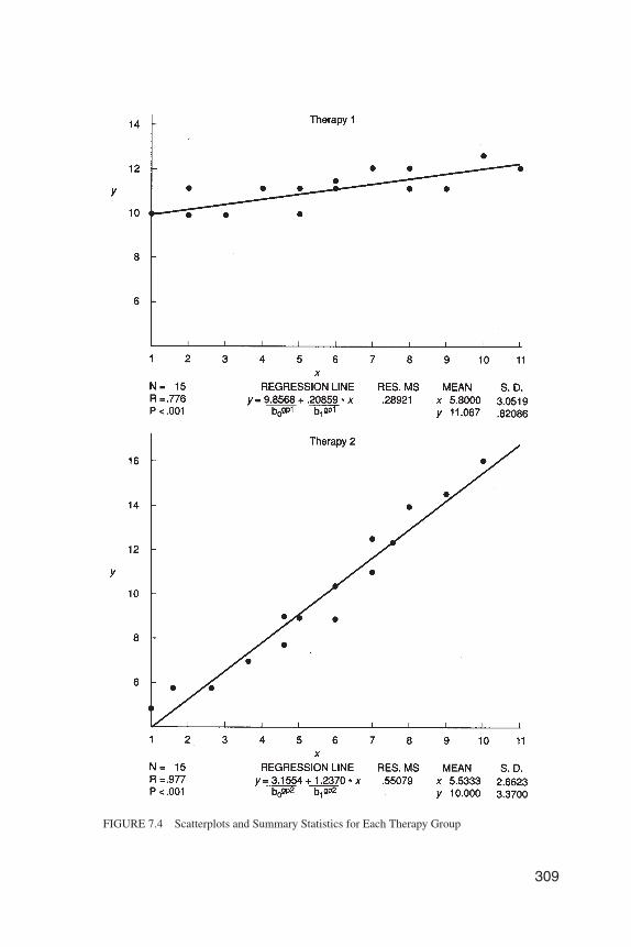
For the Huitema data, although there is a strong linear relationship in eachgroup, the assumption of equality of slopes is not tenable (Figure 7.4 shows why).Therefore, covariance is not appropriate, and we split the subjects into three levels

308 CHAPTER 7

Average reliability of two testsCorrelation between tests .50 .60 .70 .80 .90 .95

.00 .50 .60 .70 .80 .90 .95

.40 .17 .33 .50 .67 .83 .92

.50 .00 .20 .40 .60 .80 .90

.60 .00 .25 .50 .75 .88

.70 .00 .33 .67 .83

.80 .00 .50 .75

.90 .00 .50

.95 .00

309

FIGURE 7.4 Scatterplots and Summary Statistics for Each Therapy Group

310

Placeholder for T0706 from p. 331 of previous edition

TABLE 7.6Results From SPSS for Windows 12.0

for 2 × 3 Factorial Design on Huitema Data

for sociability: low (1–4), medium (4.5–7.5) and high (8–11), and set up the fol-lowing 2 × 3 ANOVA on aggressiveness:

Results from the resulting run on SPSS for Windows 12.0 are presented in Table7.6. They show, as expected, that there is a significant sociability by therapy inter-action (F = 19.735). The nature of this interaction can be gauged by examining themeans for the SOCIAL*THERAPY table. These show that for low sociabilitytherapy group 1 is more aggressive, whereas for high sociability therapy group 2 ismore aggressive. The results from the Johnson–Neyman analysis for this data, pre-sented in the first edition of this text (p. 179), show that more precisely there is nosignificant difference in aggressiveness for sociability scores between 6.04 and7.06.

7.12 USE OF SEVERAL COVARIATES

What is the rationale for using several covariates? First, the use of severalcovariates will result in greater error reduction than can be obtained with just onecovariate. The error reduction will be substantially greater if there are lowintercorrelations among the covariates. In this case each of the covariates will beremoving a somewhat different part of the error variance from the dependent vari-able. Also, with several covariates we can make a better adjustment for initial dif-ferences among groups.

Recall that with one covariate simple linear regression was involved. With sev-eral covariates (predicators), multiple regression is needed. In multiple regressionthe linear combination of the predictors that is maximally correlated with the de-pendent variable is found. The multiple correlation (R) is a maximized Pearsoncorrelation between the observed scores on y and their predicted scores, R = ryy. Al-though R is more complex it is a correlation and hence R2 can be interpreted as“proportion of variance accounted for.” Also, we will have regression coefficientsfor each of the covariates (predictors). Below we present a table comparing the sin-gle and multiple covariate cases:


SOCIABILITYLOW MEDIUM HIGH

THERAPY 1THERAPY 2

where the bi are the regression coefficients, x j1 is the mean for covariate 1 in groupj, x j2 is the mean for covariate 2 in group j, etc., and the xi are the grand means forthe covariates.

7.13 COMPUTER EXAMPLE WITH TWO COVARIATES

To illustrate running an ANCOVA with more than one covariate, we reconsider theSesame Street data set used in Section 7.9. Again we shall be interested in site dif-ferences on POSTNUMB, but now we use two covariates: PRENUMB andPRERELAT (pretest on knowledge of relational terms—amount, size, and posi-tion relationship—maximum score of 17). Before we give the control lines for run-ning the analysis, we need to discuss in more detail how to set up the lines for test-ing the homogeneity assumption. For one covariate this is equality of regressionslopes. For two covariates it is parallelism of the regression planes, and for morethan two covariates it involves equality of regression hyperplanes.

312 CHAPTER 7

TABLE 7.7SPSS MANOVA Control Lines for ANCOVA on Sesame Street Data

With Two Covariates

TITLE ‘SESAME ST. DATA-2 COVARIATES’.DATA LIST FREE/ SITE PRENUMB PRERELAT POSTNUMB.BEGIN DATA.

DATA LINES

END DATA.MANOVA PRENUMB PRERELAT POSTNUMB BY SITE(1,3)/ANALYSIS POSTNUMB WITH PRENUMB PRERELAT/PRINT = PMEANS/DESIGN/ANALYSIS = POSTNUMB/DESIGN = PRENUMB+PRERELAT,SITE,PRENUMB BY SITE+PRERELAT BY SITE/ANALYSIS = PRENUMB PRERELAT/.

One Covariate Multiple CovariatesErrorReduction

primarily determined by simplecorrelationryx

2 – within variance on yaccounted for by x

determined by the multiple correlationR2 – within variance on y accounted forby the set of covariates

Adjustmentof Means

yi* = yi—b(xi – x),b is assumed common slope

yj* = yj – b1 (x j1 – x1) – b2(x j2 – x2 ) –�

– bk(xkj – xk)

Placeholder for T 0708 from p. 334 of previous edition.

TABLE 7.8Printout from SPSS MANOVA for Sesame Data with Two Covariates

� This test indicates significant SITE differences at .05 level.� These are the regression coefficients� These are the adjusted means, which would be obtained as follows:

� This test indicates parallelism of the regression planes is tenable at the .05 level.

*3 3 1 13 1 2 23 2( ) ( )

25.437 .564(16.563 21.670 .622(8.563) 10.14)

29.30

y y b x x b x x� � � � �

� � � � �

�

It is important to recall that a violation of the assumption means there is acovariate by treatment (group) interaction. If the assumption is tenable this meansthe interaction will not be significant. Therefore, what one does in SPSSMANOVA is to set up an effect involving the interaction (for one covariate), andthen test whether this effect is significant. If the effect is significant, it means theassumption is not tenable.

For more than one covariate, as in the present case, there is an interaction termfor each covariate. The effects are lumped together and then we test whether thecombined interactions are significant. Before we give a few examples, note thatBY is the keyword used by SPSS to denote an interaction, and + is used to lump ef-fects together.

We show the control lines for testing the homogeneity assumption for twocovariates and for three covariates. Denote the dependent variable by y, thecovariates by x1 and x2 and the grouping variable by gp. The control lines are

ANALYSIS = Y/DESIGN = Xl+X2,GP,X1 BY GP+X2 BY GP /

Now, suppose there were three covariates. Then the control lines will be:

ANALYSIS = Y /DESIGN = X1+X2+X3,GP,X1 BY GP+X2 BY GP+X3 BY GP /

The control lines for running the ANCOVA on the Sesame Street data with thecovariates of PRENUMB and PRERELAT are given in Table 7.7. In Table 7.8 wepresent selected output from the SPSS analysis of covariance.

7.14 SUMMARY

1. In analysis of covariance a linear relationship is assumed between the de-pendent variable and the covariate(s).

2. ANCOVA is directly related to the two basic objectives in experimental de-sign of (a) eliminating systematic bias and (b) reduction of error variance.

While ANCOVA does not eliminate bias, it can reduce bias. The use of severalcovariates with low intercorrelations will substantially reduce error variance.

3. Limit the number of covariates (C) so that

where J is the number of groups and N is total sample size.4. A numerical example is given to show the intimate relationship between

ANCOVA and the results for ANOVA on the same data.

314 CHAPTER 7

( 1).10

C J

N

� �

�

Placeholder for T0709 from p. 337 of previous edition.

TABLE 7.9

5. Measurement error on the covariate causes loss of power in randomized de-signs, and can lead to seriously biased treatment effects in non-randomized de-signs.

6. In examining printout from the statistical packages, first make two checks todetermine whether covariance is appropriate: (1) check that there is a linear rela-tionship between the covariate and the dependent variable and (2) check that theregression slopes are equal. If either of these is not true, then covariance is not ap-propriate. In particular, if (2) is not true then the Johnson–Neyman techniqueshould be considered.

7. Several cautions are given concerning the use of analysis of covariance withintact groups.

8. Three ways of analyzing a k group pretest-posttest design are: ANOVA onthe difference scores, analysis of covariance, and a two way repeated measuresANOVA. Articles by Huck and McLean (1975) and by Jennings (1988) show thatANCOVA is generally the preferred method of analysis.

9. Although the Johnson–Neyman technique is preferred when the slopes arenot equal, it is still not available on SAS or SPSS. A violation of the equal slopesassumption means there is a group by covariate interaction effect. Because of this,we illustrated, in Section 7.12, use of a two way ANOVA to get at the nature of thisinteraction.

10. We showed how ANCOVA can be done using multiple regression. Bydummy coding group membership and appropriate multiplication we obtainedboth the test for homogeneity of regression slopes and the ANCOVA.

EXERCISES

1. A social psychological study by Novince (1977) examined the effect of be-havioral rehearsal, and behavioral rehearsal plus cognitive restructuring(combination treatment) on reducing anxiety and facilitating social skillsfor female college freshmen. The 33 subjects were randomly assigned (11each) to either BH, a control group (group 2), or BH + CR. The subjectswere pretested and posttested on several variables. The scores for theavoidance variable are given as follows:

316 CHAPTER 7

Table 7.9 shows selected printout from an ANCOVA on SPSS for Windows7.5 (top two thirds of printout).(a) Is ANCOVA appropriate for this data? Explain.(b) If ANCOVA is appropriate, then do we reject the null hypothesis ofequal adjusted population means at the .05 level?(c) The bottom portion of the printout shows the results from an ANOVAon just avoidance. Note that the error term is 280.07. The error term for theANCOVA is 111.36. How are the two error terms fundamentally related?

2. (a) Run an ANOVA on the difference scores for the data in exercise 1.(b) Compare the error term for that analysis vs the error term for theANCOVA on the same data. Relate these results to the discussion in Sec-tion 7.10.

3. This question relates the use of a pretest as covariate to experimental de-sign considerations. Suppose in a counseling study eight subjects were ran-domly assigned to each of three groups. The subjects were pretested andposttested on client satisfaction, which served as the dependent variable.(a) What is the main reason for using the pretest here as a covariate?(b) In what other way might the covariate be useful?(c) What effect would the possibility of pretest sensitization have on yourdecision to use a pretest in this study?

4. An analysis of variance is run on three intact groups and a significant dif-ference is found at the .05 level. The pattern of means is


BEHAVIORALREHEARSAL CONTROL

BEHAVIORAL REHEARSAL +COGNITIVE

RESTRUCTURING

Avoid Preavoid Avoid Preavoid Avoid Preavoid91 70 107 115 121 96107 121 76 77 140 120121 89 116 111 148 13086 80 126 121 147 145137 123 104 105 139 122138 112 96 97 121 119133 126 127 132 141 104127 121 99 98 143 121114 80 94 85 120 80118 101 92 82 140 121114 112 128 112 95 92

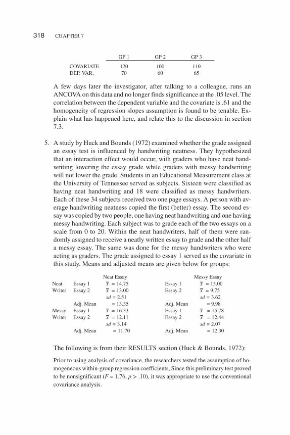
A few days later the investigator, after talking to a colleague, runs anANCOVA on this data and no longer finds significance at the .05 level. Thecorrelation between the dependent variable and the covariate is .61 and thehomogeneity of regression slopes assumption is found to be tenable. Ex-plain what has happened here, and relate this to the discussion in section7.3.

5. A study by Huck and Bounds (1972) examined whether the grade assignedan essay test is influenced by handwriting neatness. They hypothesizedthat an interaction effect would occur, with graders who have neat hand-writing lowering the essay grade while graders with messy handwritingwill not lower the grade. Students in an Educational Measurement class atthe University of Tennessee served as subjects. Sixteen were classified ashaving neat handwriting and 18 were classified as messy handwriters.Each of these 34 subjects received two one page essays. A person with av-erage handwriting neatness copied the first (better) essay. The second es-say was copied by two people, one having neat handwriting and one havingmessy handwriting. Each subject was to grade each of the two essays on ascale from 0 to 20. Within the neat handwriters, half of them were ran-domly assigned to receive a neatly written essay to grade and the other halfa messy essay. The same was done for the messy handwriters who wereacting as graders. The grade assigned to essay 1 served as the covariate inthis study. Means and adjusted means are given below for groups:

The following is from their RESULTS section (Huck & Bounds, 1972):

Prior to using analysis of covariance, the researchers tested the assumption of ho-mogeneous within-group regression coefficients, Since this preliminary test provedto be nonsignificant (F = 1.76, p > .10), it was appropriate to use the conventionalcovariance analysis.

318 CHAPTER 7

Neat Essay Messy EssayNeat Essay 1 x = 14.75 Essay 1 x = 15.00Writer Essay 2 x = 13.00 Essay 2 x = 9.75

sd = 2.51 sd = 3.62Adj. Mean = 13.35 Adj. Mean = 9.98

Messy Essay 1 x = 16.33 Essay 1 x = 15.78Writer Essay 2 x = 12.11 Essay 2 x = 12.44

sd = 3.14 sd = 2.07Adj. Mean = 11.70 Adj. Mean = 12.30

GP 1 GP 2 GP 3

COVARIATE 120 100 110DEP. VAR. 70 60 65

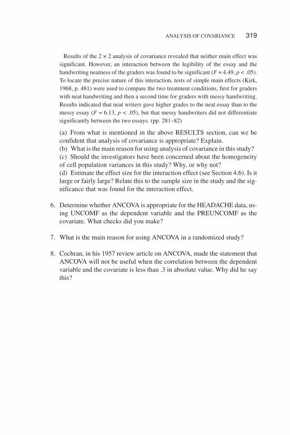
Results of the 2 × 2 analysis of covariance revealed that neither main effect wassignificant. However, an interaction between the legibility of the essay and thehandwriting neatness of the graders was found to be significant (F = 4.49, p < .05).To locate the precise nature of this interaction, tests of simple main effects (Kirk,1968, p. 481) were used to compare the two treatment conditions, first for graderswith neat handwriting and then a second time for graders with messy handwriting.Results indicated that neat writers gave higher grades to the neat essay than to themessy essay (F = 6.13, p < .05), but that messy handwriters did not differentiatesignificantly between the two essays. (pp. 281–82)

(a) From what is mentioned in the above RESULTS section, can we beconfident that analysis of covariance is appropriate? Explain.(b) What is the main reason for using analysis of covariance in this study?(c) Should the investigators have been concerned about the homogeneityof cell population variances in this study? Why, or why not?(d) Estimate the effect size for the interaction effect (see Section 4.6). Is itlarge or fairly large? Relate this to the sample size in the study and the sig-nificance that was found for the interaction effect.

6. Determine whether ANCOVA is appropriate for the HEADACHE data, us-ing UNCOMF as the dependent variable and the PREUNCOMF as thecovariate. What checks did you make?

7. What is the main reason for using ANCOVA in a randomized study?

8. Cochran, in his 1957 review article on ANCOVA, made the statement thatANCOVA will not be useful when the correlation between the dependentvariable and the covariate is less than .3 in absolute value. Why did he saythis?


Documents

Analysis of Covariance - B W Griffin · (dependent variable), say .60, we will be able to attribute 36% of the within group variance on the dependent variable to variability on I.Q