Indian Journal of Pure & Applied PhysicsVol. 42, September 2004, pp 674-683

Analysis of coupling characteristics of rectangular core optical waveguide couplerD Engles* & S S Malik**

*Department of Electronics Technology, **Department of Physics,

Guru Nanak Dev University, Amritsar 143 005Received 19 February 2004; accepted 25 May 2004

A theoretical formulism based on the boundary matching technique has been proposed to study the systematic of anasymmetric waveguide coupler. Same formulism is applicable to a symmetric coupler. The equivalent parallel coupling lengthto account for the coupling in the two S-shaped regions in the input and the output of the coupler is obtained from the couplergeometry and is dealt with more accurately and 'sensitively in our calculations. No fitting parameter is required for ourcalculation. The calculated characteristics of the asymmetric coupler are very close to those of experimental ones. Our modelcan aid in the design of diffused channel single mode rectangular core optical waveguide couplers.

[Keywords: Asymmetric couplers, Broadband couplers, Boundary matching technique]

IPC Code: H 01 P 3/20

1 IntroductionSingle mode waveguides' with rectangular cross-

section are the building blocks of the integratedoptical devices having wide range of application inoptical communication area. Among these the opticaldirectional coupler is perhaps the most important andis used to fabricate low loss optical switches, high-speed modulators, polarization converters andwavelength filters. Hence, it is quite important tostudy the coupling properties of such a directionalcoupler for their efficient design and performance.The wavelength sensitivity of an optical waveguidedirectional coupler is one of the most importantparameters as far as the performance of thecommunication system is concerned. The couplerbandwidth must accommodate the shift of the lasersource central wavelength or the spectral broadeningof the laser when modulated. Furthermore, forswitched multi-wavelength communication systemsutilizing amplifiers with gain bandwidth of the orderof 25 nm we require switches that have bandwidth atleast that large.

Channel waveguides and couplers have beentreated with a variety of theoretical techniques 1-3,9-11.

The Marcatili2 technique is the most important and isused extensively. Kumar et al.3 have modified theanalysis of Marcatili2 by including the effect of cornerregions through the first order perturbation theory. Inthis paper, we have greatly improved the technique ofKumar et at.3 and made it applicable to the symmetric

as well to the asymmetric waveguide coupler. In ourformulism , we have incorporated a technique toproperly take into account the S-shaped region in theinput and the output of the coupler, this was nOIstudied by Kumar et al.', The importance of the S·shaped region is crucial as seen in the practical designof the broadband couplers by Takagi et at.4-6. Theyhave used Beam Propagation Method (BPM)technique for obtaining the systematic of the coupler.We would like to mention that the solution givenbyBPM emphasize the beam characteristics rather thanthe modal properties of the field. A useful methodindesigning a coupler is the one, which extracts Ihecoupler performance and the field's characteristicfrom the coupler geometry. That is, it should compuethe propagation constant, the length of the parallelcoupling region for transfer of power, couplingcoefficient K, coupling efficiency 11 and the modalfields for the combined set of profile with fewmathematical simplifications and approximations.

Here, we propose a simple approximation alongwith a set of trial field for describing the propagationcharacteristics of a single mode rectangularwaveguide. The trial field enables us to defineequivalent waveguiding structure consisting of slabwaveguides. Using the equivalent guiding structure,we have obtained, in a simple way, the twofundamental vector modes EX II and PII of the originalwave guiding structure. This structure greatlysimplifies the analysis of composite guiding structure

such as 2

as asymrobtainedof the op

2 Theor;The,

asymmetAccordirformed (length Lby

Here K a

cladd

Fig. 1(b)-

Ipler

intherurel

In our[ue toin the

as notthe S-design, They:BPM)mpler.(en by~r thanhod in.ts the.risticsmputearalleluplingmodal1 fews.

alonggationagulardefinef slabicture,

twoiginalreatlyicture

ENGLES & MALIK: OPTICAL WAVEGUIDE COUPLER

suchas a directional coupler, both symmetric as wellasasymmetric configuration. The theoretical resultsobtainedby us predict the experimental behaviour'"oftheoptical waveguide coupler very nicely.

2TheoryThecross-sectional view of the symmetric and the

asymmetriccoupler is as shown in the Fig. l(a and b).Accordingto the couple mode theory' for a couplerformedof two parallel loss-less guides of interactionlengthL the power coupled into the guide II is givenby

1(2

ry=8"2Sin2(8* L)... (1)

HereK and 8 are given by:

,= {(~S~~AJ-(~'~~2)']... (2)

(a)

[;Jnlcore

I ,

n;2b! 2 [;] 2n, nl n$core

ot4 ~'lfII >-4 > "2a 2d 2a

I Ad!C.9."" ng

(b)

[;J 2. ~nl n$ n1core core

otS ~... >-4.2a. ')d ')~

1 dJ: J. - --.l.-e a Ylng

'h~:2ns

Fig.1 (a) - Two guides I and II are identical, so that 131 = 132(b)-Condition 131 f 132 can be easily realized by varying the

width of one of the guides

8=f3S-f3A =_1((f31;f32)2+1(2)... (3)

such that

1(: =1_(f31-f32 J28 f3S-f3A

... (4)

where ~I and ~2 are the propagation constants of theuncoupled waveguides I and II, respectively. ~s and~A .are the symmetric and anti-symmetric propagationconstant of the coupled guides I and II. The amplitudeterm (K2/82) represents the maximum power transferand the phase term (8*L; L being the parallel couplinglength), specifies the location of the position of themaximum power with respect to wavelength. If thetwo guides I and II are identical, so that, ~I= ~2' wehave (K2/82 =1) and 8 = K in Eq.1 Fig. l(a), thecoupling ratio will reach 100% at a particularwavelength. However, if the waveguides are notidentical, so that ~I "* ~2 (K2/82 <1), the maximumcoupling ratio cannot be 100%, therefore completepower transfer cannot take place. However, it isobserved that decrease in the power transfer results inthe broadening of the coupling efficiency responsewith respect to wavelength. The condition ~I "* ~2 canbe easily realized by varying the width of one of theguides [Fig. 1(b)].

Firstly, we determine ~I and ~2 of the individualguide with core refractive index 111 (=1.455)surrounded by a material of refractive index I1s

(1.4514, which is 0.25% less than 111), as shown in theFig. 2 (a and b). We assume that the it is a weaklyguiding structure i.e. the cladding refractive index 'l1s'

is about 0.25% less than the core refractive index n..The guide shown in the Fig. 2(b) is the perturbed

form of the actual waveguide shown in Fig. 2(a)because we choose the refractive index profile as:

n2 (x, y) = n'2 (x) + n"2 (y) - nl2

... (5)

,2 2where n (x) = ns x < -a,

2= nl •••••• -a < x < a,

2=ns x >a,

and

676 INDIAN J PURE & APPL PHYS, VOL 42, SEPTEMBER 2004

yJ"

(a)

n2 n,2 ;"'X1

'41\;2

•••2a

y (b).H

.~

~2 2 1\2 '2~2-n 2s -n1 I 1~r, ";'~A~l_..... - ...

•• ~

2 2b ..n2 n2

•...., 1 ••

~2.!m

2.·n1

2. ..• .. 2 2row

2apo. 2Ds -nt

2n

x

20,Fig, 2 - Guide shown in Fig, 2(b) is the perturbed form of the

actual waveguide shown in Fig. 2(a)

•.2 2n (y)=ns y<-b

2= nl •••••• -b < y «b,

2= ns y »-b ... (6)

The profile shown in Fig. 2(b) matches the actualprofile shown in Fig. 2(a) everywhere except thecorner regions where it differs by (n12 - n/), which isvery small. The correction in the propagation constantdue to this can be taken into account by using the first

order perturbation theory. The refractive index profilegiven in Eqs (5 and 6) enables us to solve thefollowing scalar wave equation by the method ofseparation of variables.

[;i J2 ( 2 2 f32 )]ax2 + dy2 + 1(0 n (x.y) - ljf(X,y) = 0

... (7)

where x, = 2nl'A is the wave number and ~ is thepropagation constant. Eq. (7) separates into thefollowing two equations:

[~, + k.'n"(x) -Ii.' ]x (x) = 0 ... (8)

[d2 2 "2 f3 2]di +ko n (y)- y Y(y) =0 ... (9)

with

ljf(X,y) = X(x)Y(y)

and ~x and ~y represent the separation constants andare related to propagation constant ~ as

(.l.2 (.l.2 (.l.2 k 2 2tJ = tJx + tJy - 0 n I

These solutions are given as

. .. (10)

X(x) = ABI *exp(vlx) x <-a

= AB2*coS(V2X) + AB3*sin(v2x)-a< x <a

= AB4*exp (-VIX) x> a

and

... (11)

Y(y)= Cl *exp(-vI*Y) y>b

-b < Y < b

= C4*exp(vlY)

with

... (12)y <-b

... (13)

... (14)

where ~" is ~x for Eq. (11) and ~y for Eq. (12).

Usinggiven in A(11 and 12propagatiosolving thobtained fr

(i) \jf(x,y) :2n (x,y) \jf(~

(iii) The wnormalized

00 2

fix (x)I,

The nexplicitly tGauss qua,finite integalong withFinally the(as discussethe refractiapplied usiiThe correct

YIis as give]

The COl

propagationguides in isrdetermine 1

propagationwaveguidesFig.3(a). Tperturbed f(Fig.3(a) beprofile as inHere

.2 2n (x)=ns

2=nl······-I

2=ns -1

2=nl d

profileve thenod of

... (7)

is theto the

... (8)

... (9)

.ts and

.. (10)

.. (11)

. .(12)

.. (13)

.. (14)

ENGLES & MALIK: OPTICAL WAVEGUIDE COUPLER

Using the computer program whose flow chart isgivenin Appendix A the ten arbitrary constants in Eqs(II and 12) (i.e. ABi and C; i = 1 to 4, along with twopropagationconstants ~x and ~y) are determined bysolvingthe ten simultaneous nonlinear equationsobtainedfrom the following boundary conditions;(i)ljI(x,y) and a\lf(x,y)lax continuous at x = ± a; (ii)n2(x,y) \jf(x,y) and a\lf(x,y)/ay continuous at y = ± b;(iii)The wave function given in Eqs (11 and 12) arenormalized:

00 2 00 2

Ilx (x)1 dx = 1; fIY(y)1 dy = 1

The infinite integration limit is consideredexplicitlyby using Gamma function, whereas usingGaussquadrature routine with 96 points does thefiniteintegration. The complete eigen wave functionalongwith the propagation constant ~ is determined.Finallythe correction in the propagation constant ~(asdiscussed in Appendix B) due to the difference intherefractive index profile in the edge regions isappliedusing the first order perturbation technique.Thecorrected value of the propagation constant is:

R l p.? 2 2 2)/', =1-'- +/(0 (n) =n, Y) ... (15)

y)isasgiven in Eq. B6.

The complete wave function and the correctedpropagationconstants ~I and ~2 for the individualguidesin isolation are determined. In a similar way todeterminethe symmetric and the anti-symmetricpropagationconstant of the coupler formed by the twowaveguides·we consider. the profile as shown inFig.3(a).The guide shown in the Fig. 3(b) is theperturbedform of the actual waveguide shown inFig.3(a)because we choose the refractive indexprofileas in Eq. (5).Here

,2 2n (x)=ns •••••• x<-(d+2a)),

2=11) •••••• -(d + 2al) < x < -d,

=n,2 =d <x c d ,

=n)2 d < x < d +2a2,

677

(a)y•

n2- 0,'" n2. z ~1 1 OS-

x.. "2d. 232

yA. (b)

2~' tl3 n.2 12n/-n122Dsy n. ~n.,

n,12bl ~~n2 ~'2 n12 n,21

11-:1 ~.~

2Ds2-n12 n} .~ -0 ' n2 2~2.-n12l:: 1!ll\ ~

••232

Fig. 3 - Profile shown in Fig. 3(b) matches the profile shown in

Fig.3(a)

2=ns x z-d+Za.; ... (16)

and

,,2 2n (y) = ns y <-b

2= nl •••••• -b < y < b,

2= ns y »b ... (17)

where also the above profile is shown in Fig. 3(b)matches the actual profile shown in Fig. 3(a)everywhere except in the corner region where itdiffers by (n12 - ns

2), and is very small. The correctionin the propagation constant due to this can be takeninto account by using the first order perturbationtheory.

678 INDIAN J PURE & APPL PHYS, VOL 42, SEPTEMBER 2004

Since symmetric refractive index profile along x-direction leads to two solutions of the Eq. (8), namelysymmetric (Xe) and anti-symmetric (XA) while in theY direction we have only one solution and isdescribed by Eq. 12.

These X solutions are given as

Xs(x) = Al "exp(v.x) x < -(d+2a])

= A4*exp(v]x) + A5*exp(v]x) -d« x < d

= A8*exp(-v]x)

and

... (18)

= B4*exp (v.x) - B5*exp(v]x) -d< x < d

= B8*exp (-v]x) ... (19)

Y(y) solutions are same as in Eq. (12) and here V],

V2 are as given in the Eqs (13 and 14), where ~" nowis ~xsfor Eq. (18), ~xAfor Eq. (19) and ~y for Eq. (12).

The twenty-three arbitrary constants in Eqs (18,19 and 12) (i.e. Ai, B; and q; i =1 to 8, j =1 to 4 alongwith three propagation constants ~xs, ~XAand ~y) aredetermined by solving the twenty-three simultaneousnon-linear equations obtained from the followingboundary conditions.

(i) \jf(x,y) and d\jf(x,y)ldX continuous at x = ± d, x =d+2a2 and x = -( d+Za.). (ii) n2(x,y) \jf(x,y) andd\jf(x,y)ldy continuous at y = ±b. (iii) The wavefunction given in Eqs (18, 19, and 12) are normalized:

00 2 00 2 00 2

SIXxs(x)1 dx=l;SIXxA(x)1 dx=l;SIY(y)1 dy=l

The complete wave function along with ~s, and~Ais determined.

... (20)

The correction in the propagation constant duetothe difference in the refractive index profile in theedge regions is applied:

f3 2 f32 2 (2 2c = + K 0 n] - n2 )y 2

with Y2 given in appendix B Eq. B7.

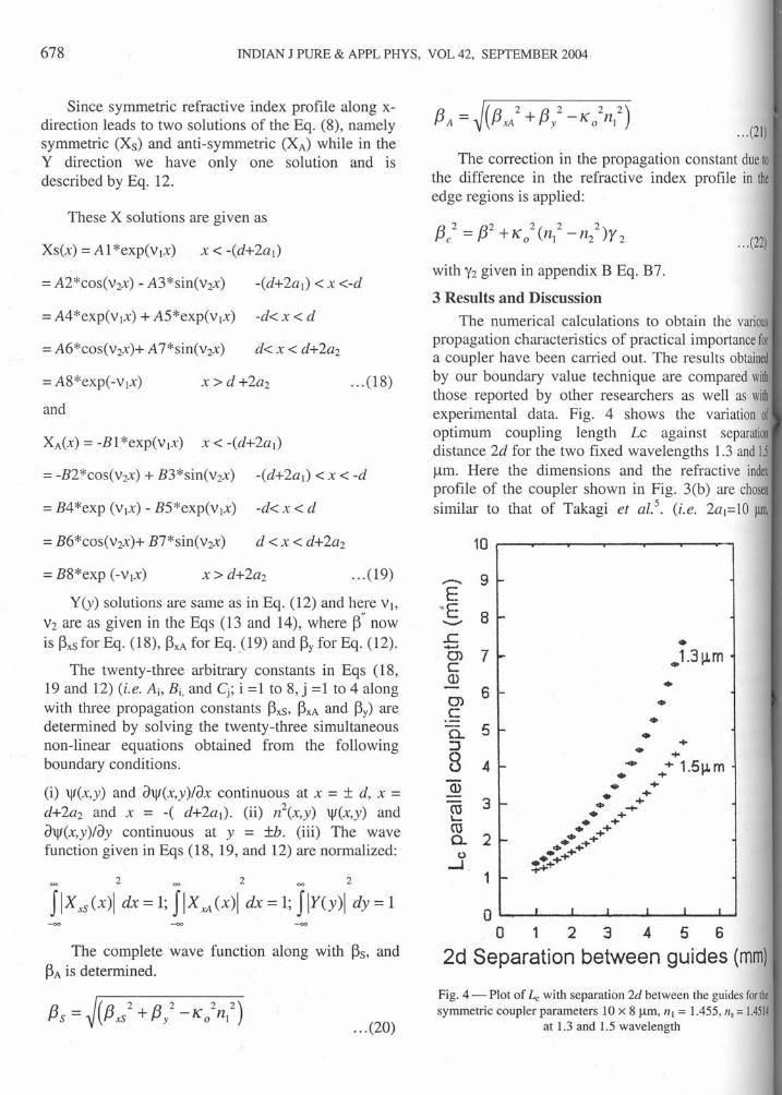
3 Results and DiscussionThe numerical calculations to obtain the various

propagation characteristics of practical importance fora coupler have been carried out. The results obtainedby our boundary value technique are compared withthose reported by other researchers as well as wiiliexperi.mental data. Fig. 4 shows the variation ofoptimum coupling length Lc against separationdistance 2d for the two fixed wavelengths 1.3 and l.lurn. Here the dimensions and the refractive indexprofile of the coupler shown in Fig. 3(b) are chosensimilar to that of Takagi et al.'. (i.e. 2a]=10 ~m,

.-.... 9E

"E 8 -•.....•.•£: •.•...en 7 I- ...1.3~mcCD •••6 I-CJ) •••c: •••CL 5 •••:::J ...8 ••• ...

4 - .. .•..•.1.5j.Lm•••

03 ••• ...• ...

3 !- ••• ...ro ..•..

••• +'- • +ro ••• ++0- 2 !- .•. ...

••••• -t-0 • ++...J ••.•.+-1J+"

1 -o ~--~--I~~~--~--~I--_~'

0123456

2d Separation between guides (mm)

Fig. 4 - Plot of Lc with separation 2d between the guides for thesymmetric coupler parameters 10 x 8 um, III= 1.455, Il,= 1.4514

at 1.3 and 1.5 wavelength

... (21)

... (22)

2a2=8 urn,good agreeThis comtechniqueFurther cocompariso:wavelengtlshown inchosen sirexactly sirr3.1 Incremerregion

A pra:couplers usthe Fig. 6coupling stthe straightas we movgiven coupand has to IL of the strthis coupliroutput ascoupling lei

The COI

be written a

where L isand I1l'is th

0.8i0.7

0.6>-oc 0.5<ll'0IE

0.4W0>.Sa. 0.3 ~::-:::J0U 0.2

0.1

01.1

Fig.5-Wavecoupling length

.. .(21)

nt due toIe in the

... (22)

variousance forobtainedred withas withition ofparationand 1.5e indexchosen

10 urn,

nm)

for the1.4514

ENGLES & MALIK: OPTICAL WAVEGUIDE COUPLER 679

1a~8urn, 2b=8 urn, Sn = 0.25%). Our results are ingood agreement with those shown in Fig. 7 of Ref. 5 .Thiscomparison strengthens the validity of ourIeChniquefor designing an asymmetric coupler.Furtherconfirmation of our technique arises from thecomparisonof the coupling efficiency 11 againstwavelengthA plot for different interaction lengths asmownin Fig. 5. Again the coupler parameters arechosensimilar to that of Ref. 8. Our results areexactlysimilar with those shown in Fig. 2 of Ref. 8.

11Incremental parallel coupling length due to S-shapedI!gion

A practical waveguide type of the directionalcouplersusually have two S-shaped arms as shown inilie Fig. 6, in the input and the output where thecouplingstrength gradually increases as we approachilie straightparallel region and decrease at the outputas wemove away from it. To design a coupler for apvencoupling ratio this coupling cannot be neglectedand hasto be taken into account in deciding the lengthLofthe straight parallel coupling region. We refer tothiscoupling in the curvature region at the input andoutputas a coupling over an incremental parallelcouplinglength M!.

Thecoupling efficiency for the coupler now canlie writtenas:

K2~=82Sin2 (8( L + ~R))

... (23)

whereL is the length of the parallel coupling regionand i1l'is the incremental parallel coupling length that

O.B rl ---------------------,

0] ---l~~m-.----..--..---0.6

/-/. l.4mm-Iig 0.51isW 0.4ocT, 0.3Joo 0.2

?'/:~

~::-~-:~ 1.7mm

--,- -.m

-_ 2.0 mm- ..•.0' - --t.t 1.2 1.3 1.4 1.5 1.6 1.7

Wavelength ((j.Jm)

Fig. 5- Wavelength response of asymmetric coupler for variouscouplinglengths Land 2at = 8 urn, 2a2 = 61lm, 2b = 81lm, 2d = 3

urn, H, = 1.455, Hs = 1.4514

L x LP.-2"~-F- P,2d-r: y - •. z

~ ~~2a2t \R R" ~ PI

Fig. 6 - Geometry of the coupler with the two S - shaped armsof the radius R in the input and the output. L is the parallelcoupling length and L is the length of the curved arm, from

the edge that contribute to the coupling

accounts for the coupling in the two S-shaped regions(over the length L) in the input and the output. Wehave to determine /)./ for designing an asymmetric

coupler for maximum efficiency.

The curvature regions are formed by bending thewaveguide into an arc of a circle, this introduceslosses. These losses depend on the radius of curvatureR of the arc as well as the refractive index differencebetween the core and the cladding". Smaller is R thelarger is the loss and for a given radius smaller thedifference between the refractive index of the coreand the cladding larger is the loss. Since we areassuming that the waveguides in our case are weaklyguiding so to keep the losses low it is expected that alarge radius arc be used. Radius cannot be madearbitrarily large, as this will increase the overall sizeof the coupler. It is seen that for a SiOr Ti02 planerwaveguide formed on a silicon substrate withrefractive index difference of 0.25% between the coreand the cladding, a radius of curvature of the order of50mm is suitable as the bending losses in this case areless" than O.3dB.

Once the radius is fixed, we determine the phasechange (8*z) that occurs in the curved region in thedirection z. This is estimated by treating the twowaveguides as a series of short sections of parallelwaveguides of length z with separation between thetwo guides for each section increasing as we moveaway from the central parallel region (as a series ofsteps). This is consistent with the fact that whilefabricating curved waveguides or diagonal lines inoptical integrated circuits a staircase type of functionis utilized which implements the curved portion or thediagonal line as a series of short steps. If there are nsteps then using the above formalism, 8, for each stepis determined and hence the total phase change thatoccur in the n steps of length z each is given by

680 INDIAN J PURE & APPL PHYS, VOL 42, SEPTEMBER 2004

= Z L· 8. (. 1 2 3 )I I 1 = , , n ... (24)

For a complete power/maximum power transferfrom guide I to II, total phase change that is requiredis n/2 and this happens when the parallel couplinglength is equal to the optimum length L; Using theabove formulism the optimum coupling length at agiven wavelength is determined and thus theincremental parallel coupling length that accounts forthe coupling in the two S-shaped regions in the inputand the output for a given guide geometry and at agiven wavelength is:

(2Lc )!::,.£ = 2 -;-CZLi 8J ._

(1 - 1,2,3 n) ... (25)

The next step is to fix the length z of each section.By making several run of the program using differentvalues of z we find that for z less than 1.5 urn thechange in ~t is very small (at the third place of

decimal). We have chosen z = 1 urn. Thus for movinga distance z along the arc of the circle of radius R therequired change in the angle at the center is

88; = sin' 1 (z*R)

Taking 8 = 0 at the edge of the central parallelregion, we increase the angle 8 in steps of 88; anddetermine the separation between the two guides foreach section and then determine the phase change foreach section. Summing up the phase change for eachsection the incremental parallel coupling length isdetermined as described above. It may be added herethat if a staircase function is being used in fabricationthe curved portion of the waveguide is then the stepsize assumed in the staircase function can be takenequal to z with a minor modification in the program.

The upper limit of the total number of steps i.e. nis fixed at a point where the coupling coefficient K

between the two guides vanishes. It is worthwhile tomention here that Takagi et al.6 have chosen aconstant value tL; = 1.2 mm away from the edge ofthe parallel coupling region). In our case L; is not aconstant value but it varies with A for a given couplergeometry.

This choice of L, makes our formulism morepracticable. Thus to calculate the incrementalcoupling length we take z =1 urn, we increase theangle in steps of 88;, (starting with 88; = 0, for thisvalue we calculate Le) and determining 2d the

separation for each section. For this value of 2d wedetermine 8 and K. We make a summation of all 0;tillfor a value of 2d, K is less than 1*10-10

• From thisvalue of 8; the phase change in the curvature regionisdetermined and hence the incremental coupling lengthis determined from the Eq. (25). A plot of 111 with

wavelength is as shown in the Fig. 7.

~t = 0.63 mm at A = 1.3 urn, and is in good

agreement with the experimental data shown inRef. (5) Finally, we have calculated the variation of~t with radius of curvature R and is as shown in

Fig. 8. The dots on the same plot represent theexperimental results as shown by Takagi et al.5

,

Fig. 8. Our theoretical results are very close to theexperimental data.

Rig. 9 shows the coupling efficiency withwavelength for different parallel coupling lengthscorrected for the coupling in the two S-shaped regionsin the input and .the output. The lines are thecalculated theoretical curves obtained due to theabove formulism while the points are theexperimental data points as given in Fig. 14 of Ref.(5). It can be seen that the theoretical curves in ourcase match those of Fig. 6 in Ref. (5) and the

800.-----..----.---.....-----,c------,...-...EE---

800

//

.://

/

//--I

!

750 I-

....J<l..c+-'0>CQ)....J

SCQ)

EQ)L- .oc

700 I-

650 ,.....

550

500 L-~I~~' ~J __ ~J __ L_'_~'~1 1.1 1.2 1.3 1.4 1.5 1.6 1.7

Wavelength (IJm)Fig. 7 - Variation of incremental coupling length Uwith

wavelength, for the coupler with parameters 2al = 8 um,2a2 = 6 11m,2b = 811m, 2d = 311m, nl = 1.455, ns = 1.4514

\

E'1.0E::; 0.8<i..c.0,0.6c<l)...J

CO0.4.•...c<l)E 0.2bE 0.0

a

Fig.8-Varcurvature f

0.7

0.1

0.6

.Q 0.51i5c::: 0.4OJ.sg. 0.3oo

o1

Fig.9-PIL, the corret

811m,2a20.25% less

experimenagreementmay be dithat even imm in Ftheoreticalthat for thefficiencyrange 1.3-flat as thecoupling tlhave rerno

f 2d weall 8; till'om thisegion isg lengthD...t with

m goodown ination oftown in

ent theet ai.5,

~ to the

y withlengthsregionsare theto the

re theof Ref.; 10 ourmd the

/

1.7

'with

,LLm,

4514

\

ENGLES & MALIK: OPTICAL WAVEGUIDE COUPLER 681

E'1.0E~0.8<Ji0,0.6cQ)oJ

mOA•..cQ)

~0.2bc-no. 0:;--1£',---!;'::---L- .

) "(;",;;:--_.1.' _ II

20 40 60 80 100Radius of Curvature, R (mm)

Fig.8-Variation of incremental coupling length t..lwith radius ofcurvaturefor the coupler with parameters 2 a,=8 J.l1TI,2a2=6J.lm,

2b = 8 urn, 2d= 3J.l1TI,11,=1.455, 112=1.4514

j•0.71 ,, __ - __ L Tmm __

0.6-'//. ..

0.5Q

i /,'~ 0.4 •• / _..CI /_ _ •••..•••••£ ./- • <,~ 0.3 /:;.-. ., "-8 // ~-------...... ........~2mm02

.i->: -. • -c , ••••<,

. ~ ....

..

Therefore, our calculated results are improved 10

comparison to those given in Ref. (5).

»:

4 Conclusion

In this paper using the boundary value techniquewe made a detailed theoretical investigation of thecoupler with emphasis on the wavelength flatteningcharacteristics. The propagation constant and themodal fields for the combined set of profile arecomputed with as few mathematical simplificationsand approximations as possible. We compare ourresults with those of the experimental results ofRefs (4-6) and find that these are in good agreement.While fabricating curved waveguides or diagonallines in optical integrated circuits a staircase type offunction is utilized which implements the curvedportion or the diagonal line as a series of short steps.If a staircase function is being used to fabricate thecurved portion of the S-shaped arm of the waveguidethen the step size assumed in the staircase functioncan be taken equal to z with a minor modification inour program to determine the equivalent parallelcoupling length to account for the coupling in the twoS-shaped arms in the input and the output. One pointthat needs to be mentioned here is the computingtime. The computing time to determine the equivalentparallel coupling length for one wavelength is of theorder of 5 to 6 min. We are using a simple Pentiumbased PC at 700 MHz. A higher configuration willreduce the time considerably.

.9 mm

'..0.1 <,

1.6

References

Murphy T E, PhD thesis, Department of ElectricalEngineering and Computer Science, (MIT Cambridge) 2001.

2 Marcatili E J A, Bell System Techl1 J, 48 (1969) 2071.3 Kumar A, Kaul A N & Ghatak A K, Optics Leu, 10 (1985)

86.4 Takagi A, Jinguji K & Kawachi M, IEEE J Quantum

Electronics, 28 (1992) 848.5 Takato N, Jinguji K, Yasu M, Toba H & Kawachi M, IEEE J

Lightwave Techn, 6 (1988) 1003.6 Takagi A, Jinguji K & Kawachi M, IEEE J Lightwave Techn,

10 (1992) 735.7 Takagi A, Jinguji K & Kawachi M, IEEE J Lightwave Tecl1l1,

10 (1992) 1814.8 Takagi A, Jinguji K & Kawachi M, Electronic Leu, 26

(1990) 132.9 Little BE & Murphy T, IEEE Photonics Tech Lett, 9 (1997).10 Liang T & Ziolkowski R W, IEEE Photonics Tech Left, 10

(1998).11 Kwan Chung Ho & Chiang K S, IEEE J Light Wave Tech, 20

(2002).

''''. 1.5mm01 t [ t ,- ••.••.•. ,.

1 1.1 1.2 1.3 1.4Wavelength (urn)

1.5

Fig.9- Plot of coupling efficiency with wavelength for variousL,(he corrected coupling length, the coupler parameters are 2a, =

81-1In,2a2 = 6 urn, 2b = 8 urn, 2d = 3 urn, 11, = 1.455 and I1sis0.25% less than n,. The points are the experimental data points

from Ref. (4) Fig. 14

experimentalpoints fit onto these curves with goodagreementexcept for the curve for L = 1.2 mm. Thismaybe due to some experimental error as it is seenIhaleven in Ref. (5) the experimental curve for L=1.2mmin Fig.14 Ref. (5) does not agree with theIheoreticalcurve in Fig. 6 Ref. (5). It can also be seenIhatfor the coupler with L = 0.9 mm, the couplingefficiencyis about 50% ± 5 within the wavelengthrange1.3-1.5 urn. The curves become more and moreflalas the coupling efficiency decreases i.e. for weakcouplingthe matching is exact. In our calculation wehaveremoved the arbitrariness in the choice of L;

682\

INDIAN J PURE & APPL PHYS, VOL 42, SEPTEMBER 2004

Matrix ill

Conditioned

Appendix A

n - The number of non-linear equations; E I - Theminimum pivot magnitude allowed in the Gauss-Jordan reduction; E2- A small positive number usedin convergence test; XIQ ••••••••••. xno- The initial guess

for given root; imax - Maximum number of Newton.Rapson iterations; itcon Convergence testparameter.

Flow chart of the program to solve the twenty.three non-linear equations to determine the twentyconstants and f3xs, f3XAand f3y

Evthlat Eltmmt5 &..

'"Aug:emtnttd Matrix

T/"d=O

salvennon linear eon4>(:xj.)&c = -f(ljJfor increment

C\,determent dF

itcon = 0

T ..••-------'

C onv ergenc ek,d,n

X,l.-+1·····x...l.-+1

The wave eq

where

In the cormdifference (= nl2

be written as

where

'Jf = 'Vo + C'VI

f32 = {32 + E{32p () I

and

Substitutingwe get

Ho'Vl+ H''Vo={3o

Multiplyingthe total area 0

the propagation

or

_ENGLES & MALIK: OPTICAL WAVEGUIDE COUPLER

r of Newton-Tgence test

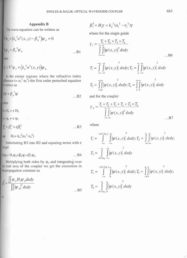
Appendix BThewave equation can be written as

the twenty-the twenty

1 (2 2 f3 2)11f!0+kon(x,y)- a If/o=O

Holf!o= f302lf/ a ... BI

~here

Ho= '\12 If!0+ (ko 2n2 (X, Y))lf/ a

In the corner regions where the refractive indexaifference(= n]2_ns

2) the first order perturbed equationre writtenas

HIf! = f3 /If! ... B2

where

H=Ho+EH]

W=ljIo+E\jf]

p~= f3~ + Ef3]2 ... B3

and H]= ko2(n]2-ns

2)

Substituting B3 into B2 and equating terms with E

weget

HoljI]+ H]\jfo=~o\jf]+~]\jfo ... B4

Multiplying both sides by \jfo and integrating overIhetotal area of the coupler we get the correction inIhepropagation constant as

2 If If! a H]lf/ .dxd»~]==-=--:-:-------

IlIlf/012

dxdy... BS

or

f32 2 2 2] = H]y = ko (n] - n, )y

where for the single guide

~+Tz+~+~y] = --'----=---"----'-

f fllf/(x, y)12dxdy... B6

-a, -b 2 ee =b 2

t; = f fllf/(x,y)1 dxdy.T, = f fllf/(x,y)1 dxdya~

2 2+a=

t; = f fllf/(x, y)1 dxdy; t; = f fllf/(x, y)1 dxdy~b a b

and for the coupler

_~+Tz+~+~+Ys+'4,Y2 - oo oo

f fllf/(x,y)12

dxdy

where

T=]-(d+2a,) =b 2 d -b 2

f fllf/(x,y)1 dxdy;Tz = f fllf/(x,y)1 dxdy;-d~

2

.r; =~ -b

f fllf/(x, y)1 dxdyd+2a2 ~

-(d+2a,) oo 2 d cc 2

t; = f fllf/(x,y)1 dxdy;T; = f fllf/(x,y)1 dxdy;b -db

_ _ 2

'4,= f fllf/(x,y)1 dxdy(/+2a2 b

683

... B7

j,