Embed Size (px)
Citation preview
Analysis of Contour Motions
Ce Liu William T. Freeman Edward H. Adelson
Computer Science and Artificial Intelligence Laboratory
Massachusetts Institute of Technology
Neural Information Processing Systems 2006
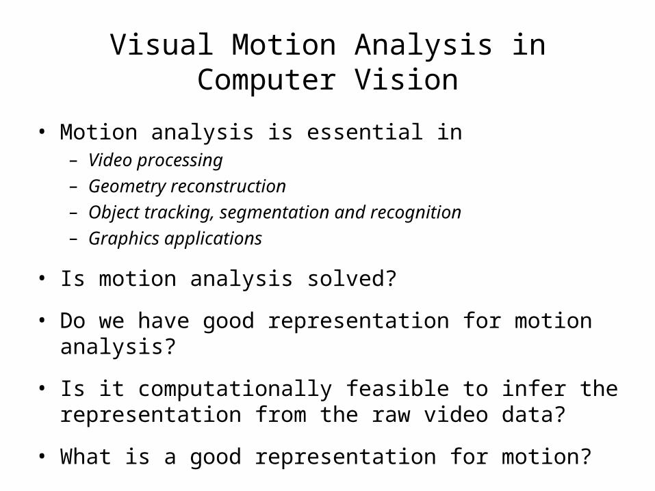
Visual Motion Analysis in Computer Vision
• Motion analysis is essential in– Video processing – Geometry reconstruction– Object tracking, segmentation and recognition– Graphics applications
• Is motion analysis solved?
• Do we have good representation for motion analysis?
• Is it computationally feasible to infer the representation from the raw video data?
• What is a good representation for motion?
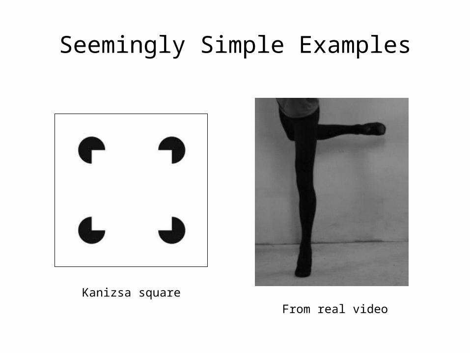
Seemingly Simple Examples
Kanizsa square
From real video
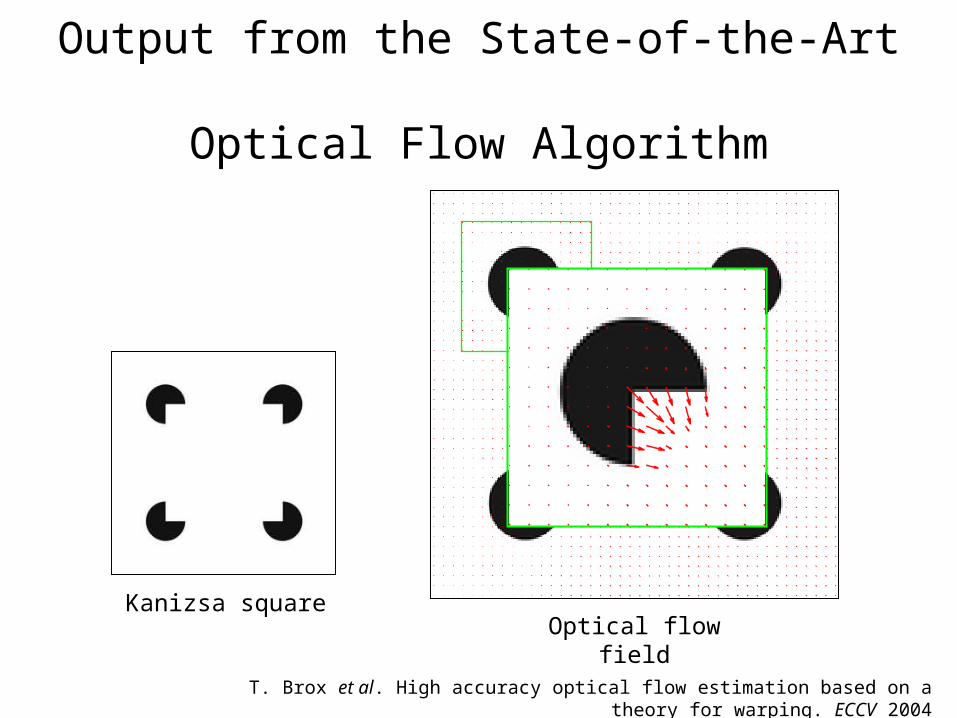
Output from the State-of-the-Art Optical Flow Algorithm
T. Brox et al. High accuracy optical flow estimation based on a theory for warping. ECCV 2004
Optical flow fieldKanizsa square
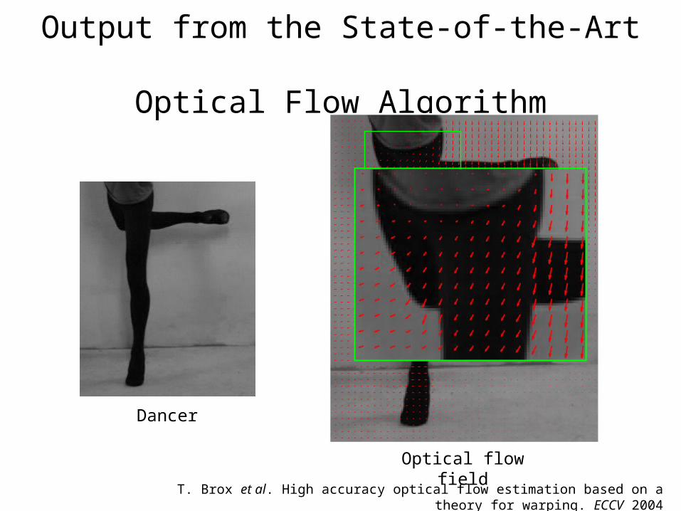
Output from the State-of-the-Art Optical Flow Algorithm
T. Brox et al. High accuracy optical flow estimation based on a theory for warping. ECCV 2004
Optical flow field
Dancer
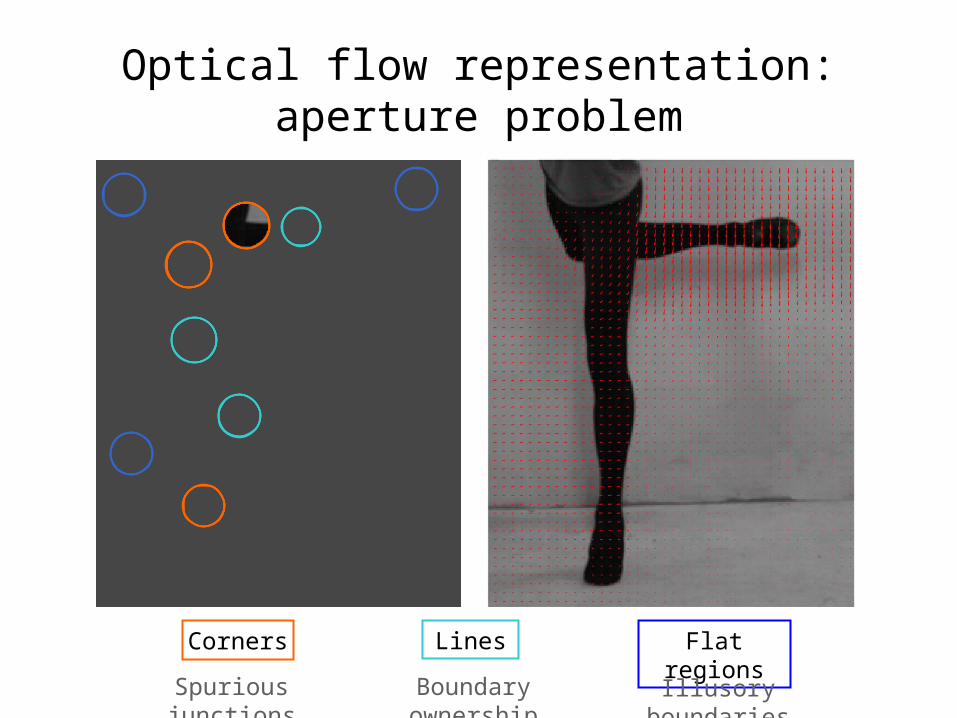
Optical flow representation: aperture problem
Corners Lines Flat regions
Spurious junctions Boundary ownership Illusory boundaries
Optical Flow Representation
Corners Lines Flat regions
Spurious junctions Boundary ownership Illusory boundaries
We need motion representation beyond pixel level!
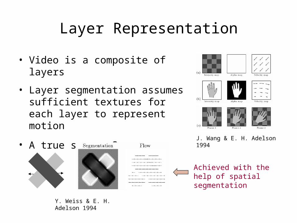
Layer Representation
• Video is a composite of layers
• Layer segmentation assumes sufficient textures for each layer to represent motion
• A true success?
J. Wang & E. H. Adelson 1994
Y. Weiss & E. H. Adelson 1994
Achieved with the help of spatial segmentation
Layer Representation
• Video is a composite of layers
• Layer segmentation assumes sufficient textures for each layer to represent motion
• A true success?
J. Wang & E. H. Adelson 1994
Y. Weiss & E. H. Adelson 1994
Achieved with the help of spatial segmentation
Layer representation is good, but the existing layersegmentation algorithms cannot find the right layersfor textureless objects
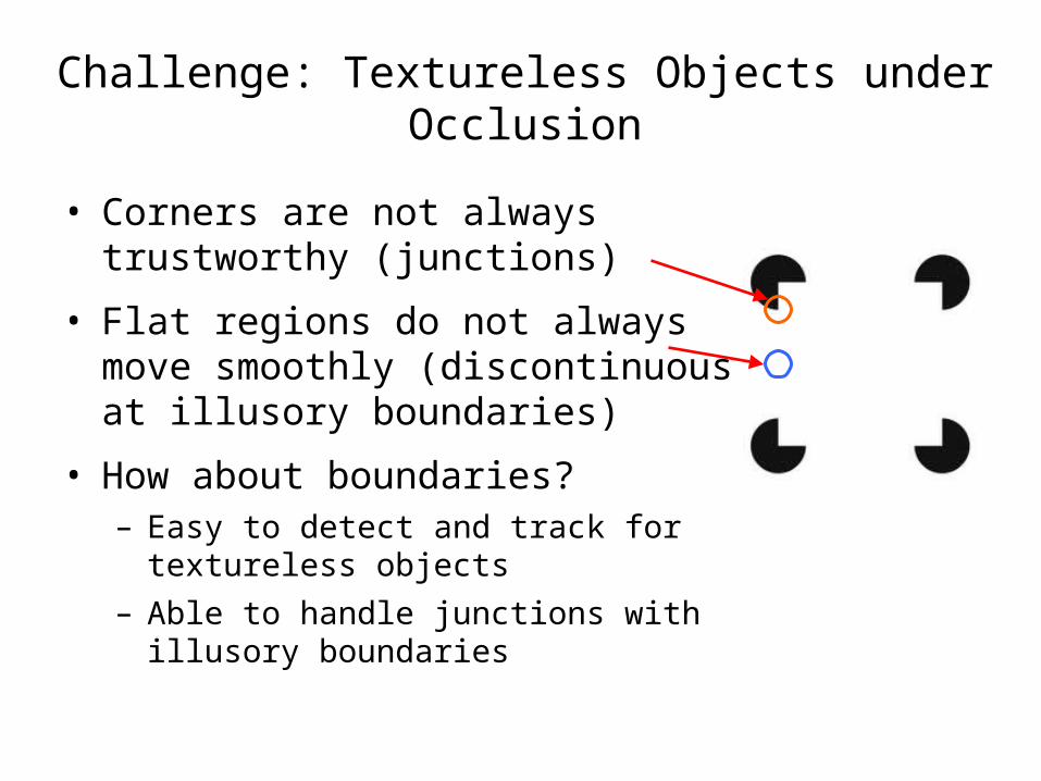
Challenge: Textureless Objects under Occlusion
• Corners are not always trustworthy (junctions)
• Flat regions do not always move smoothly (discontinuous at illusory boundaries)
• How about boundaries?– Easy to detect and track for textureless
objects
– Able to handle junctions with illusory boundaries
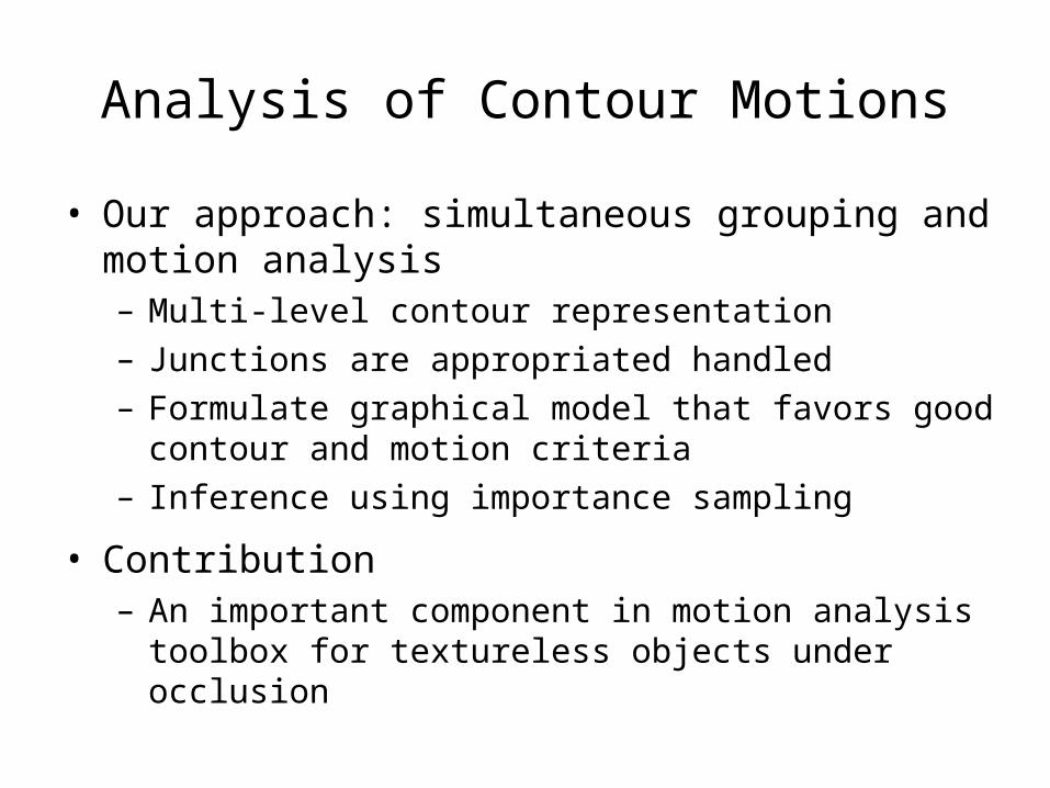
Analysis of Contour Motions
• Our approach: simultaneous grouping and motion analysis– Multi-level contour representation
– Junctions are appropriated handled
– Formulate graphical model that favors good contour and motion criteria
– Inference using importance sampling
• Contribution– An important component in motion analysis toolbox for
textureless objects under occlusion
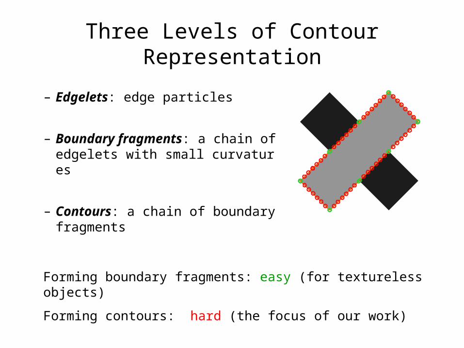
Three Levels of Contour Representation
– Edgelets: edge particles
– Boundary fragments: a chain of edgelets with small curvatures
– Contours: a chain of boundary fragments
Forming boundary fragments: easy (for textureless objects)
Forming contours: hard (the focus of our work)
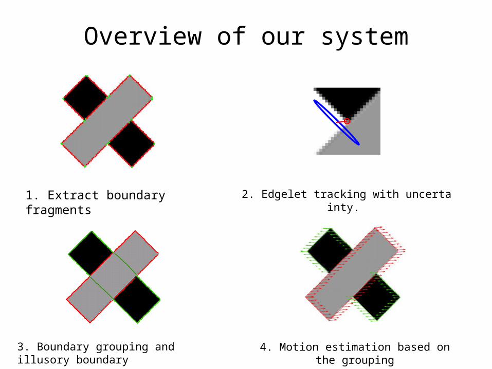
Overview of our system
1. Extract boundary fragments 2. Edgelet tracking with uncertainty.
3. Boundary grouping and illusory boundary 4. Motion estimation based on the grouping
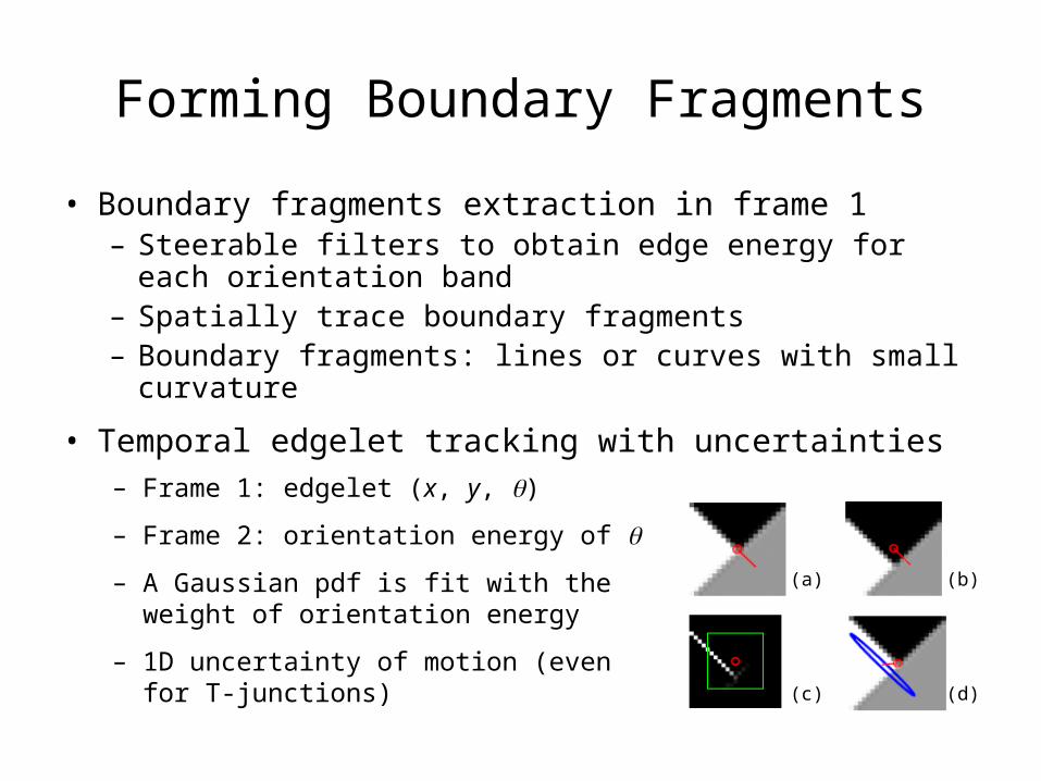
Forming Boundary Fragments
• Boundary fragments extraction in frame 1– Steerable filters to obtain edge energy for each
orientation band– Spatially trace boundary fragments– Boundary fragments: lines or curves with small curvature
• Temporal edgelet tracking with uncertainties
(a) (b)
(c) (d)
– Frame 1: edgelet (x, y, )
– Frame 2: orientation energy of
– A Gaussian pdf is fit with the weight of orientation energy
– 1D uncertainty of motion (even for T-junctions)
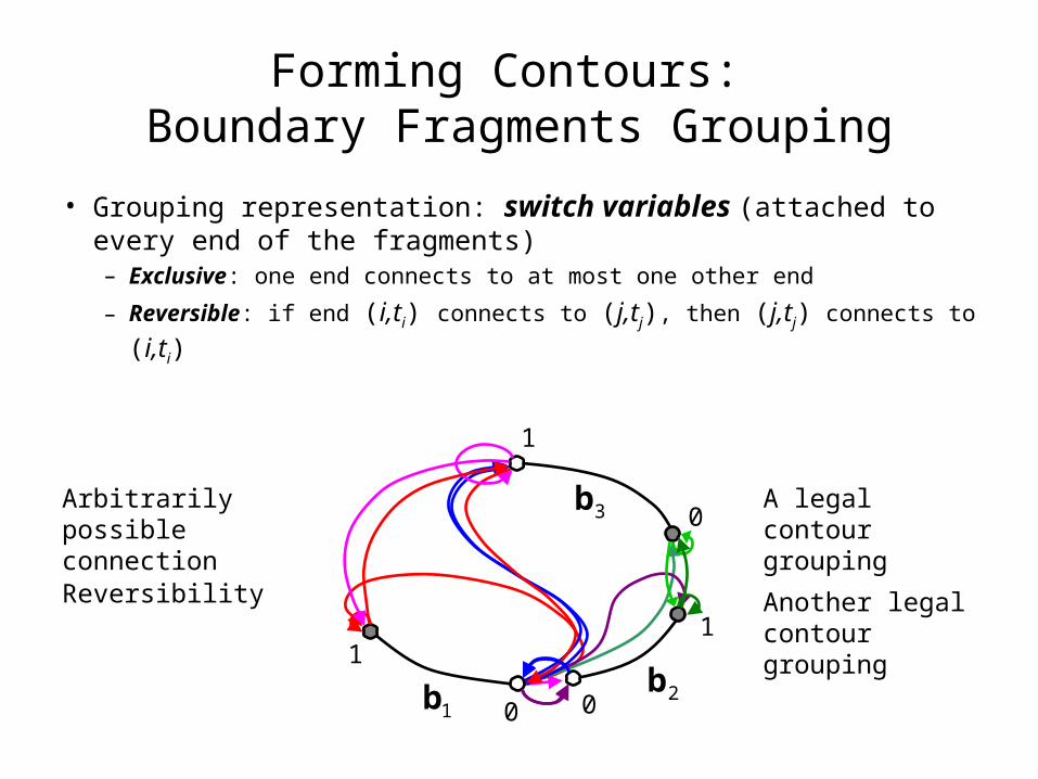
Forming Contours: Boundary Fragments Grouping
• Grouping representation: switch variables (attached to every end of the fragments)– Exclusive: one end connects to at most one other end
– Reversible: if end (i,ti) connects to (j,tj), then (j,tj) connects to (i,ti)
Arbitrarily possible connection
1b 2b
3b
Reversibility
A legal contour grouping
Another legal contour grouping
0
1
0
1
1
0
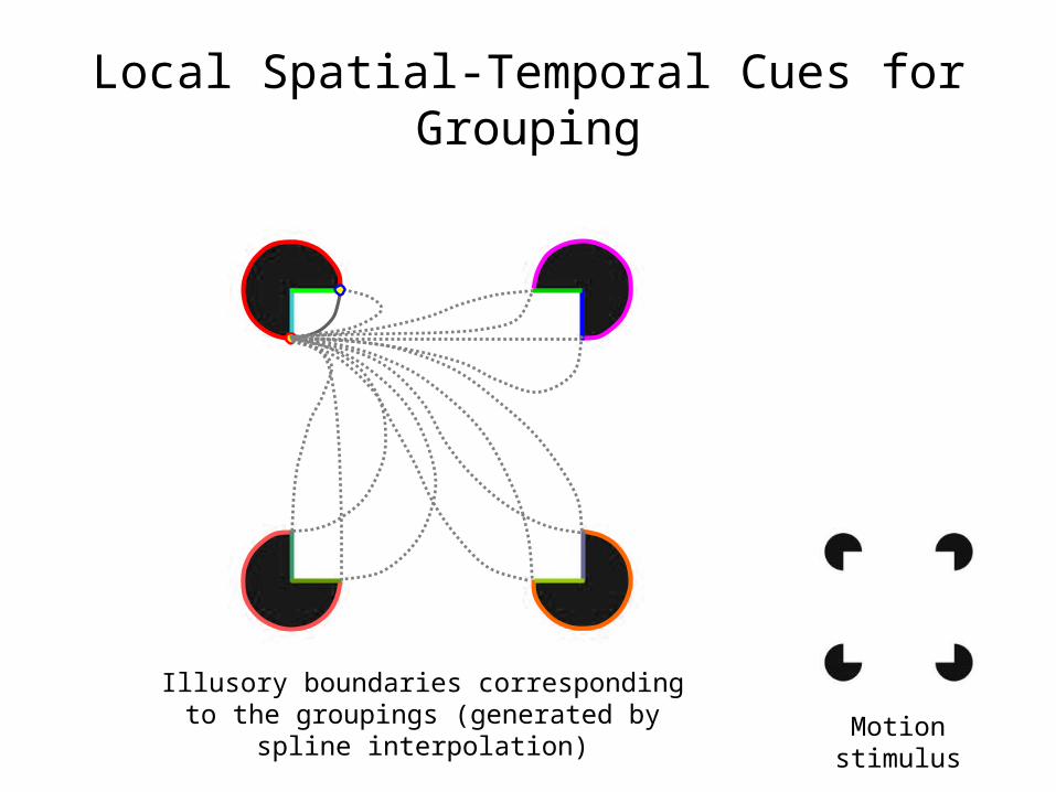
Local Spatial-Temporal Cues for Grouping
Motion stimulus
Illusory boundaries corresponding to the groupings (generated by spline interpolation)
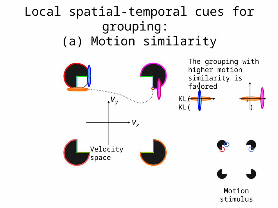
Local spatial-temporal cues for grouping: (a) Motion similarity
Motion stimulus
xv
yv
Velocity space
KL( ) < KL( )
The grouping with higher motion similarity is favored
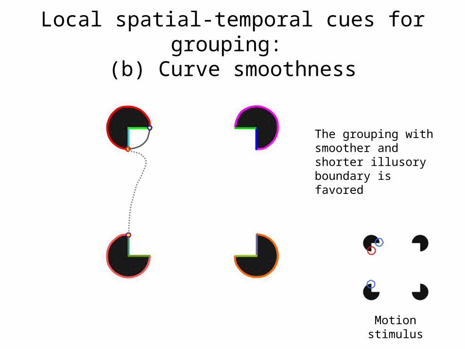
Local spatial-temporal cues for grouping: (b) Curve smoothness
Motion stimulus
The grouping with smoother and shorter illusory boundary is favored
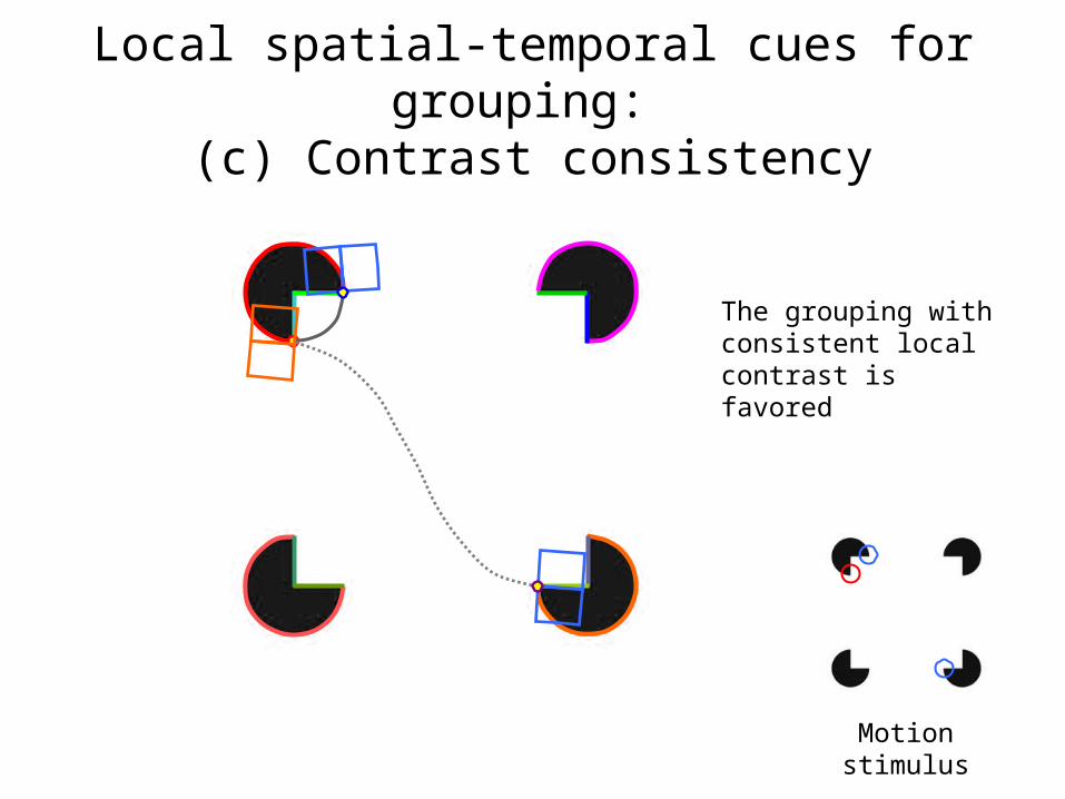
Local spatial-temporal cues for grouping: (c) Contrast consistency
Motion stimulus
The grouping with consistent local contrast is favored
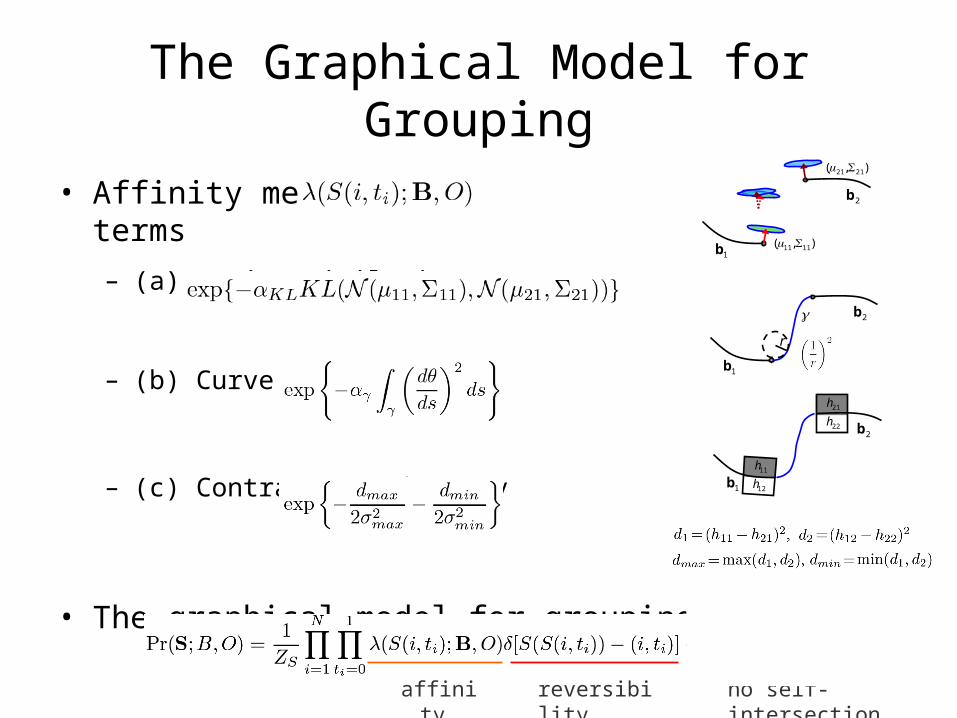
The Graphical Model for Grouping
• Affinity metric terms
– (a) Motion similarity
– (b) Curve smoothness
– (c) Contrast consistency
• The graphical model for grouping
1b
2b
),( 1111
),( 2121
1b
r
2b
reversibilityaffinity
11h
12h
21h
22h
1b
2b
no self-intersection
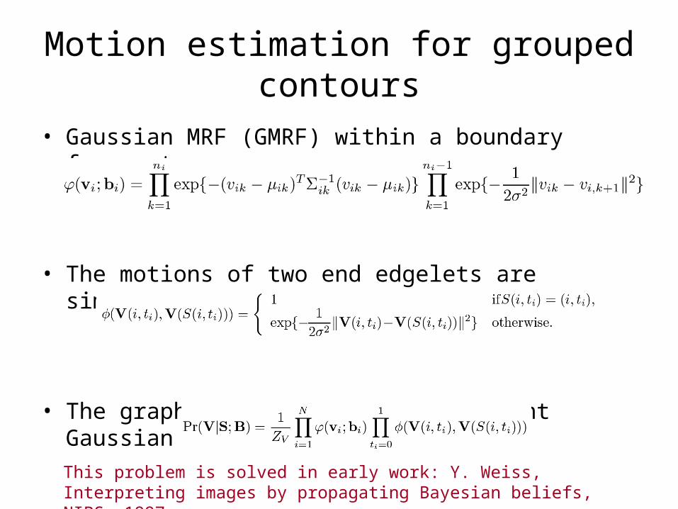
Motion estimation for grouped contours
• Gaussian MRF (GMRF) within a boundary fragment
• The motions of two end edgelets are similar if they are grouped together
• The graphical model of motion: joint Gaussian given the grouping
This problem is solved in early work: Y. Weiss, Interpreting images by propagating Bayesian beliefs, NIPS, 1997.
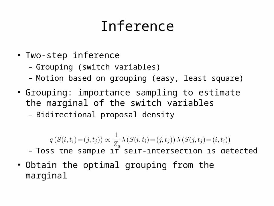
Inference
• Two-step inference– Grouping (switch variables)
– Motion based on grouping (easy, least square)
• Grouping: importance sampling to estimate the marginal of the switch variables– Bidirectional proposal density
– Toss the sample if self-intersection is detected
• Obtain the optimal grouping from the marginal

1b2b
3b4b
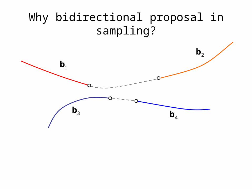
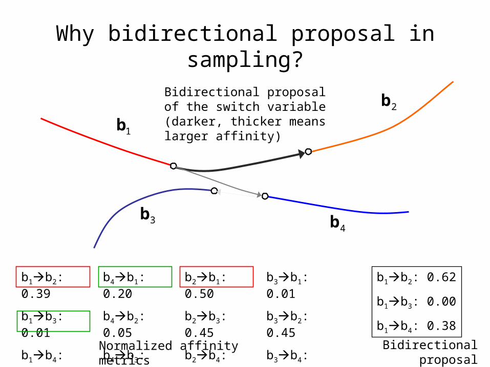
Why bidirectional proposal in sampling?
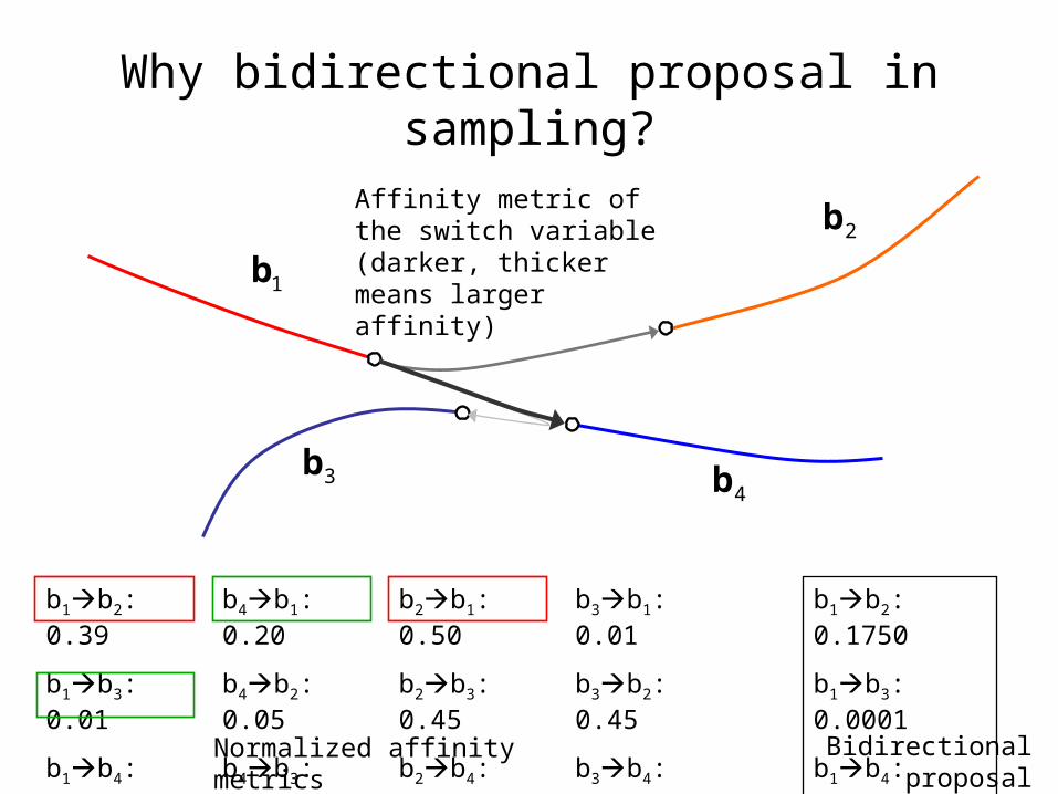
Why bidirectional proposal in sampling?
1b2b
3b4b
b1b2: 0.39
b1b3: 0.01
b1b4: 0.60
Normalized affinity metrics
b4b1: 0.20
b4b2: 0.05
b4b3: 0.85
b2b1: 0.50
b2b3: 0.45
b2b4: 0.05
b3b1: 0.01
b3b2: 0.45
b3b4: 0.54
b1b2: 0.1750
b1b3: 0.0001
b1b4: 0.1200
Affinity metric of the switch variable (darker, thicker means larger affinity)
Bidirectional proposal

Why bidirectional proposal in sampling?
b1b2: 0.39
b1b3: 0.01
b1b4: 0.60
Normalized affinity metrics Bidirectional proposal(Normalized)
b4b1: 0.20
b4b2: 0.05
b4b3: 0.85
b2b1: 0.50
b2b3: 0.45
b2b4: 0.05
b3b1: 0.01
b3b2: 0.45
b3b4: 0.54
b1b2: 0.62
b1b3: 0.00
b1b4: 0.38
Bidirectional proposal of the switch variable (darker, thicker means larger affinity)
1b2b
3b4b
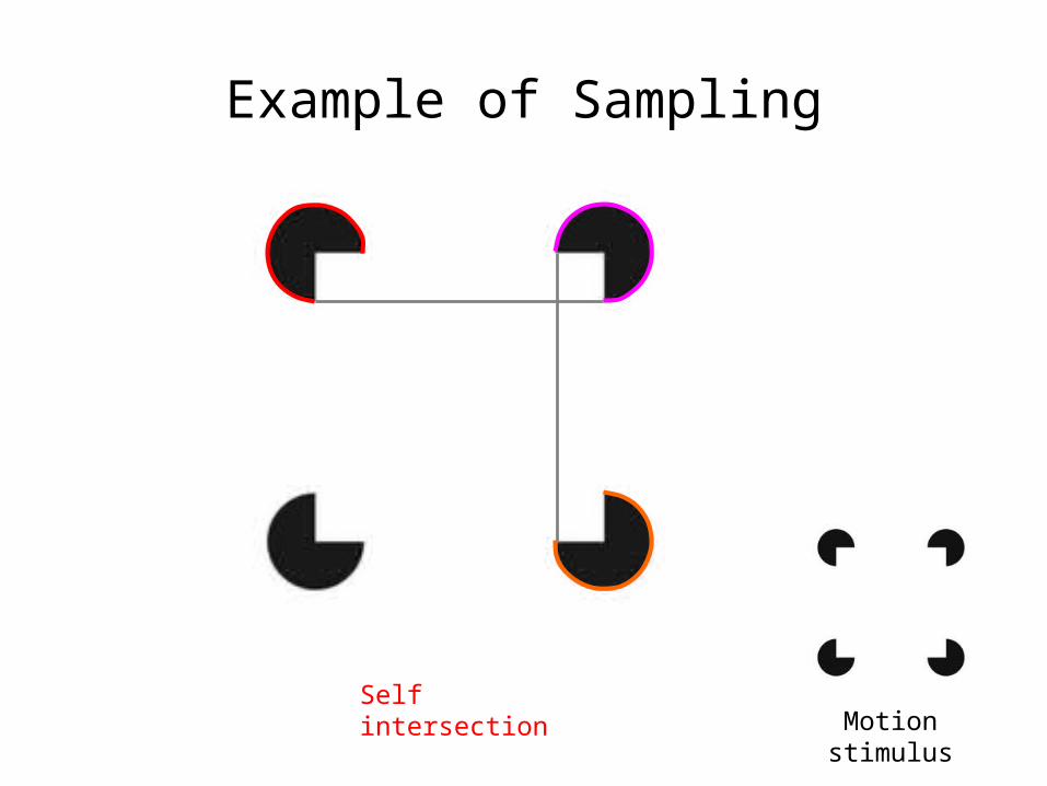
Example of Sampling
Motion stimulusSelf intersection
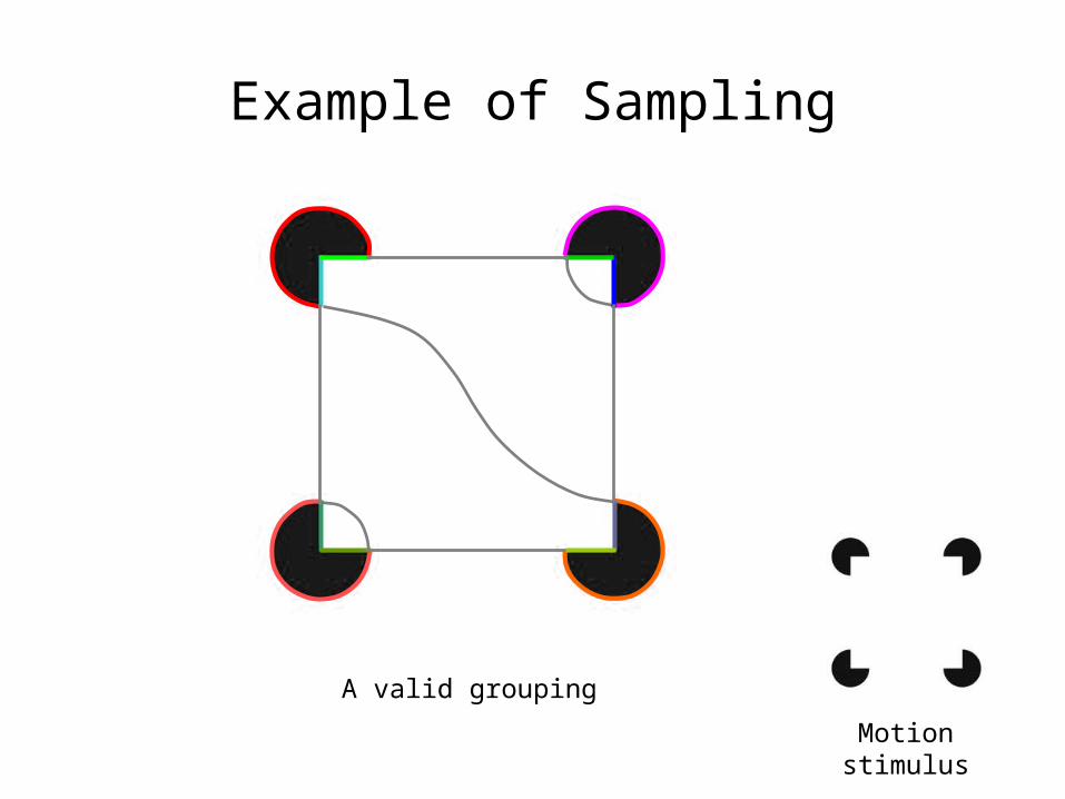
Example of Sampling
Motion stimulus
A valid grouping
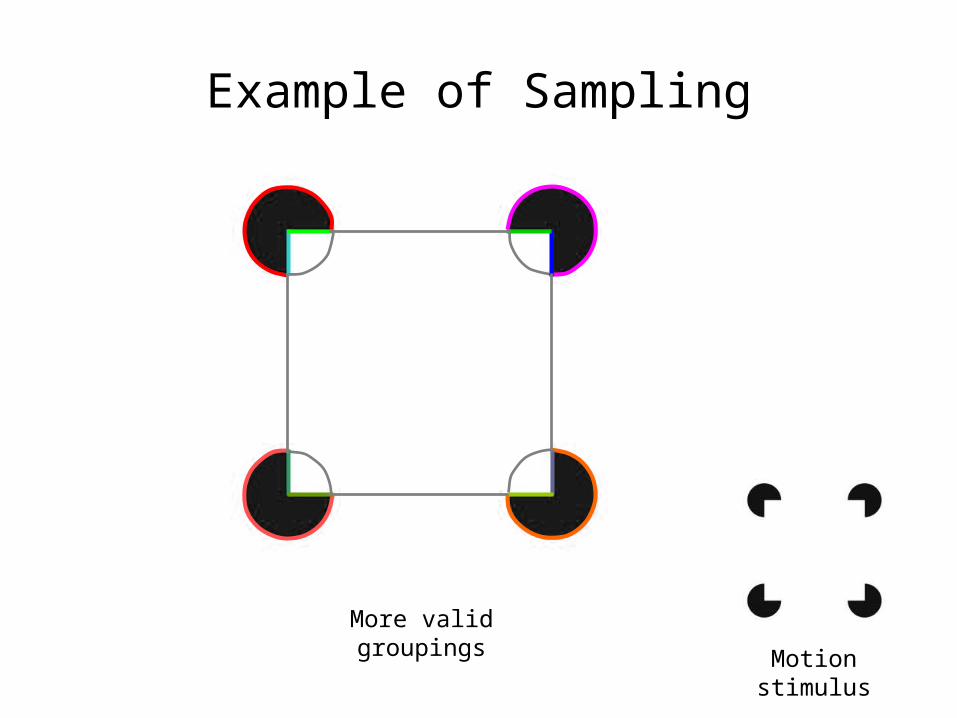
Example of Sampling
Motion stimulus
More valid groupings
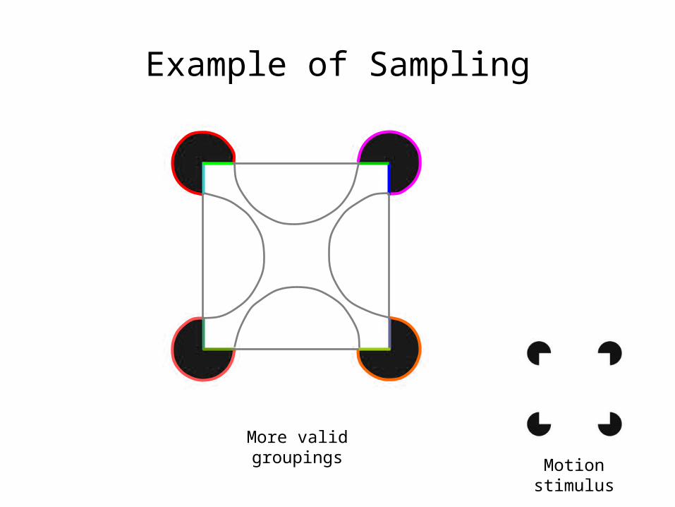
Example of Sampling
Motion stimulus
More valid groupings
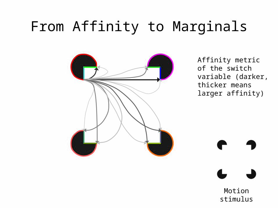
From Affinity to Marginals
Affinity metric of the switch variable (darker, thicker means larger affinity)
Motion stimulus
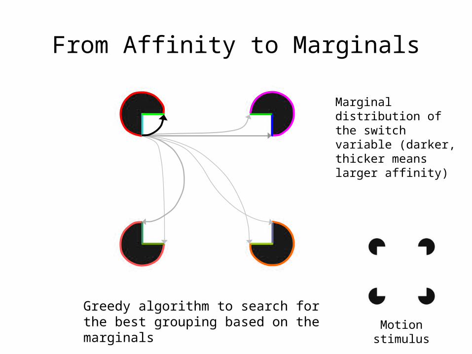
From Affinity to Marginals
Marginal distribution of the switch variable (darker, thicker means larger affinity)
Motion stimulus
Greedy algorithm to search for the best grouping based on the marginals
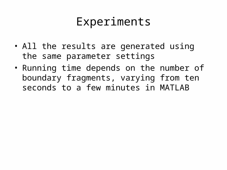
Experiments
• All the results are generated using the same parameter settings
• Running time depends on the number of boundary fragments, varying from ten seconds to a few minutes in MATLAB
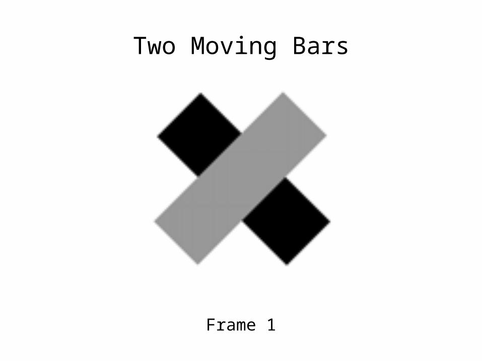
Frame 1
Two Moving Bars
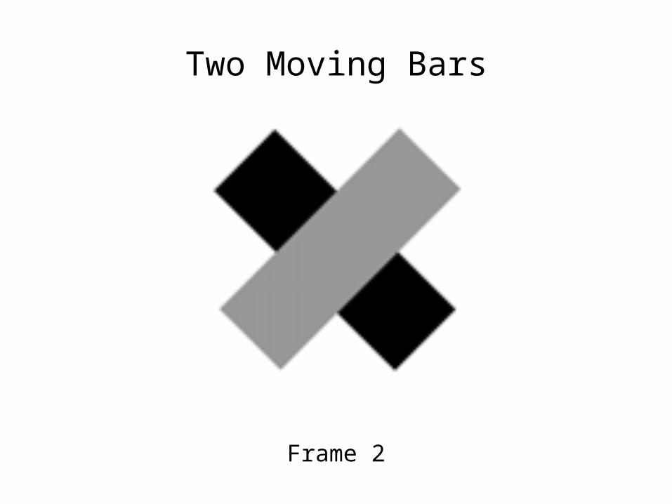
Frame 2
Two Moving Bars
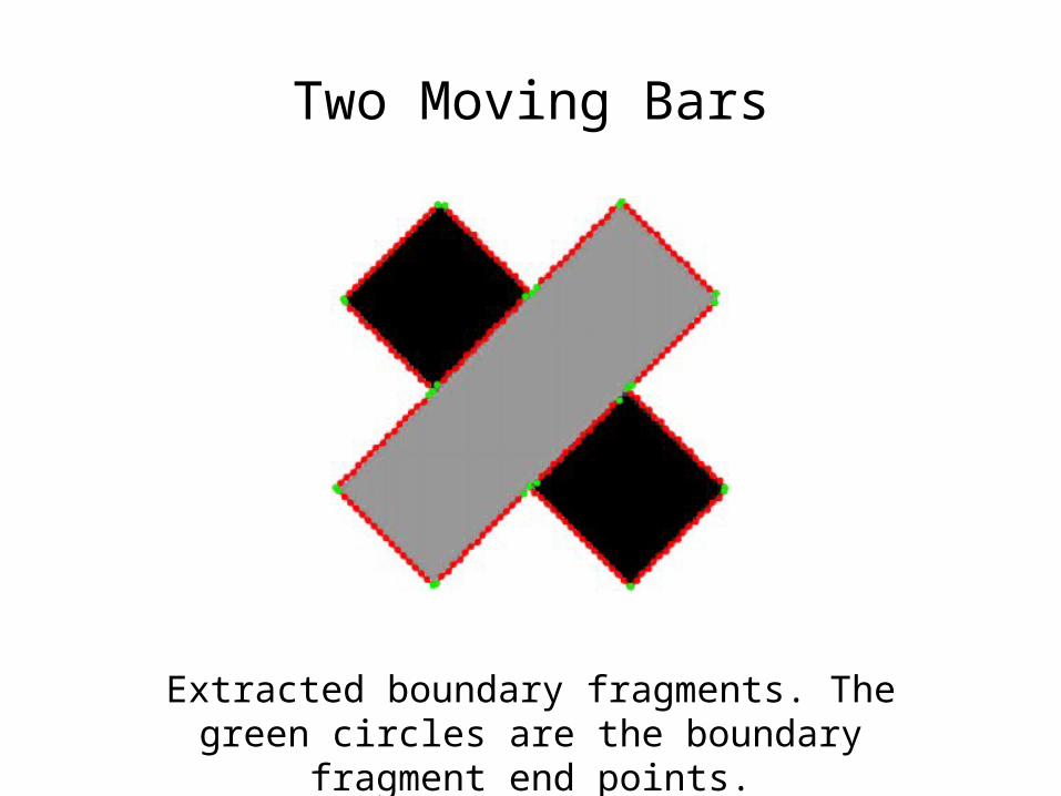
Extracted boundary fragments. The green circles are the boundary fragment end points.
Two Moving Bars
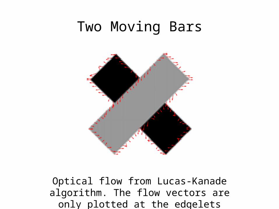
Optical flow from Lucas-Kanade algorithm. The flow vectors are only plotted at the edgelets
Two Moving Bars
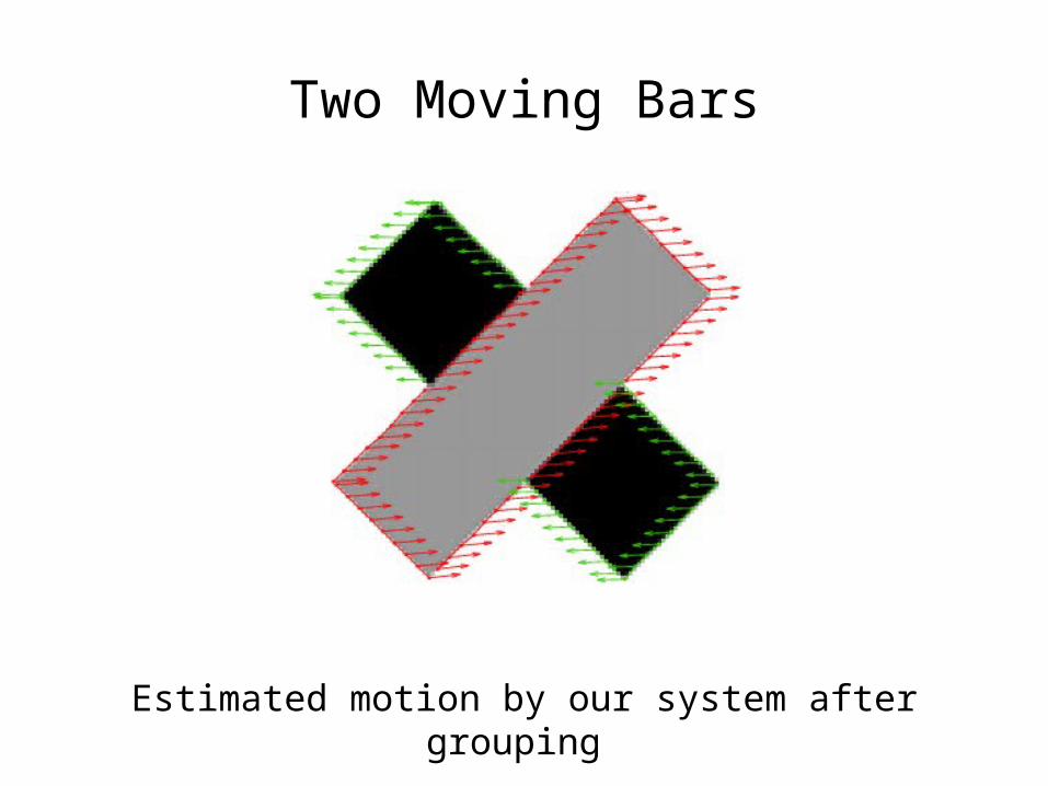
Estimated motion by our system after grouping
Two Moving Bars
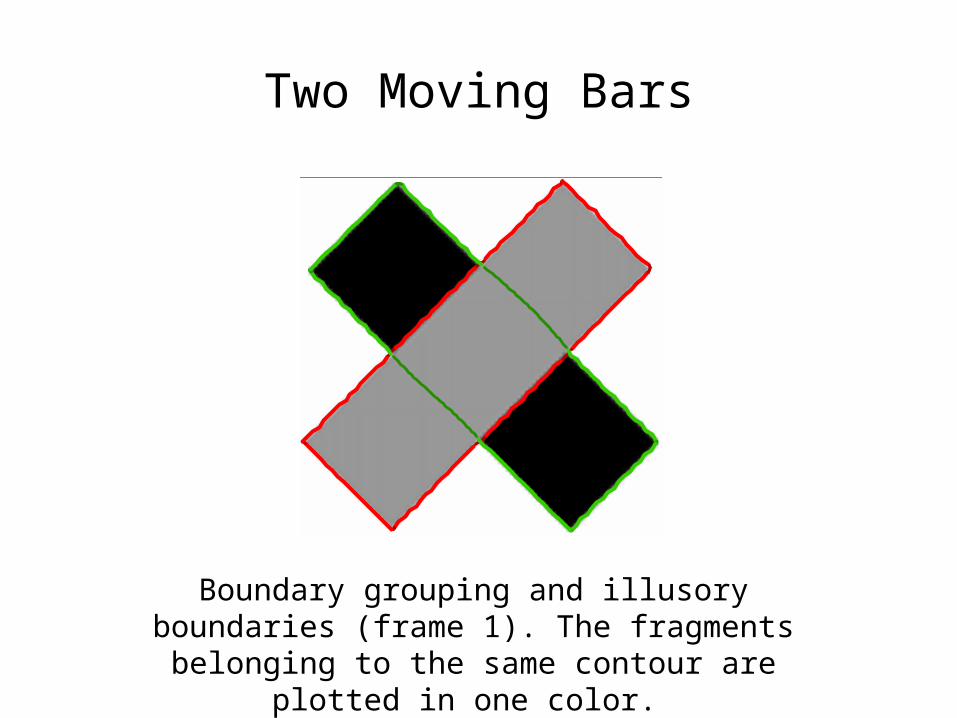
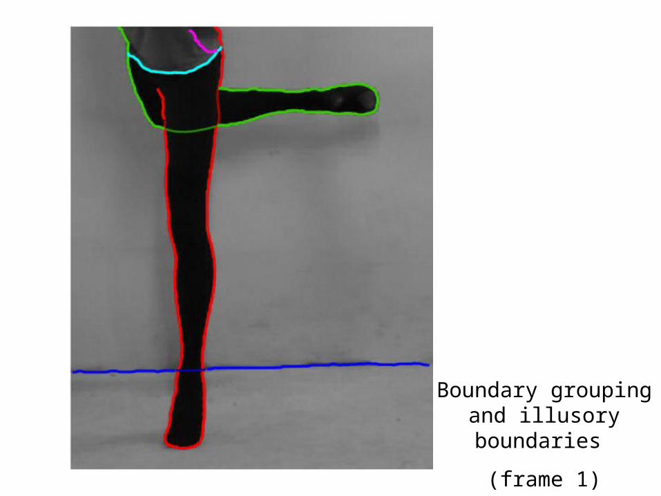
Boundary grouping and illusory boundaries (frame 1). The fragments belonging to the same contour are
plotted in one color.
Two Moving Bars
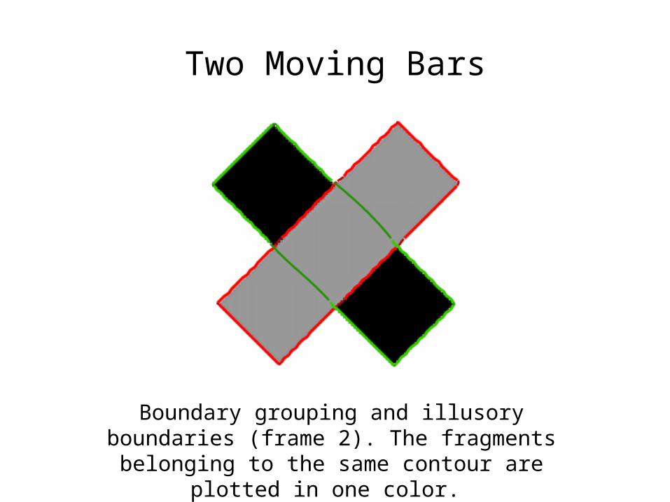
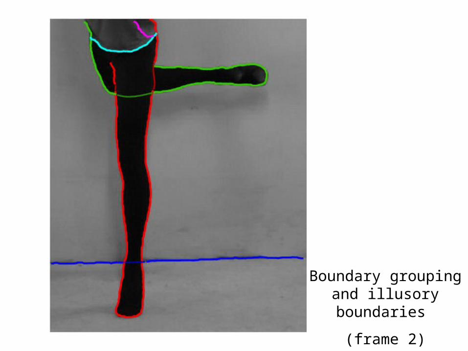
Boundary grouping and illusory boundaries (frame 2). The fragments belonging to the same contour are
plotted in one color.
Two Moving Bars

Kanizsa Square
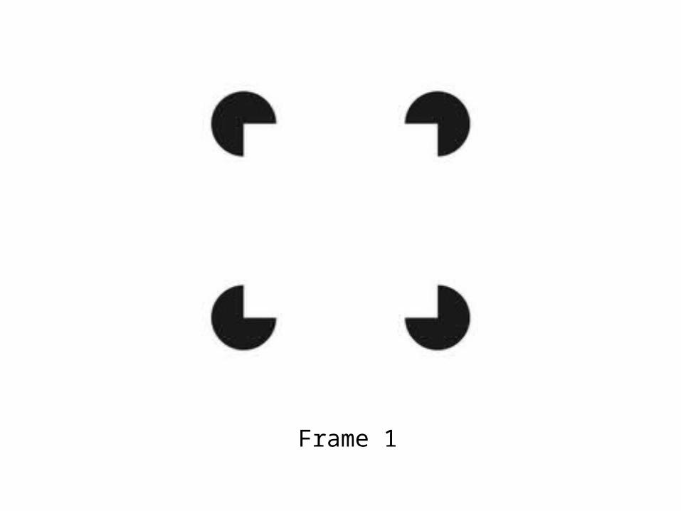
Frame 1
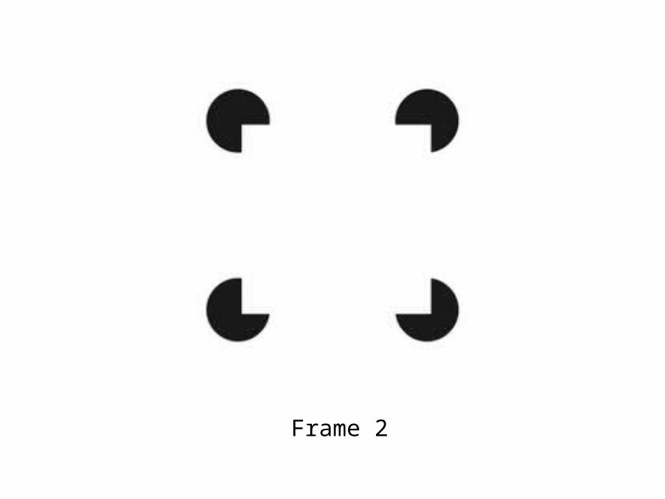
Frame 2
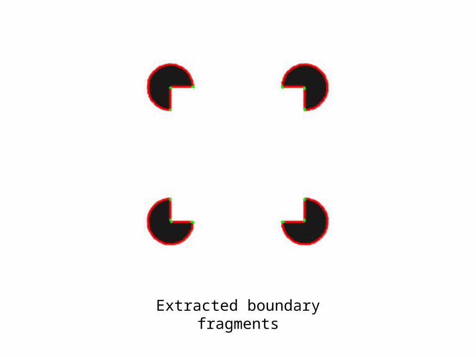
Extracted boundary fragments
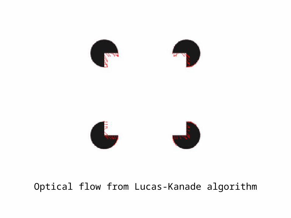
Optical flow from Lucas-Kanade algorithm
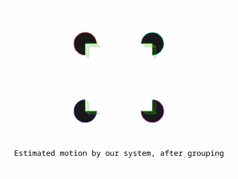
Estimated motion by our system, after grouping
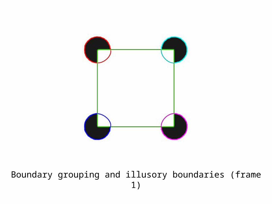
Boundary grouping and illusory boundaries (frame 1)
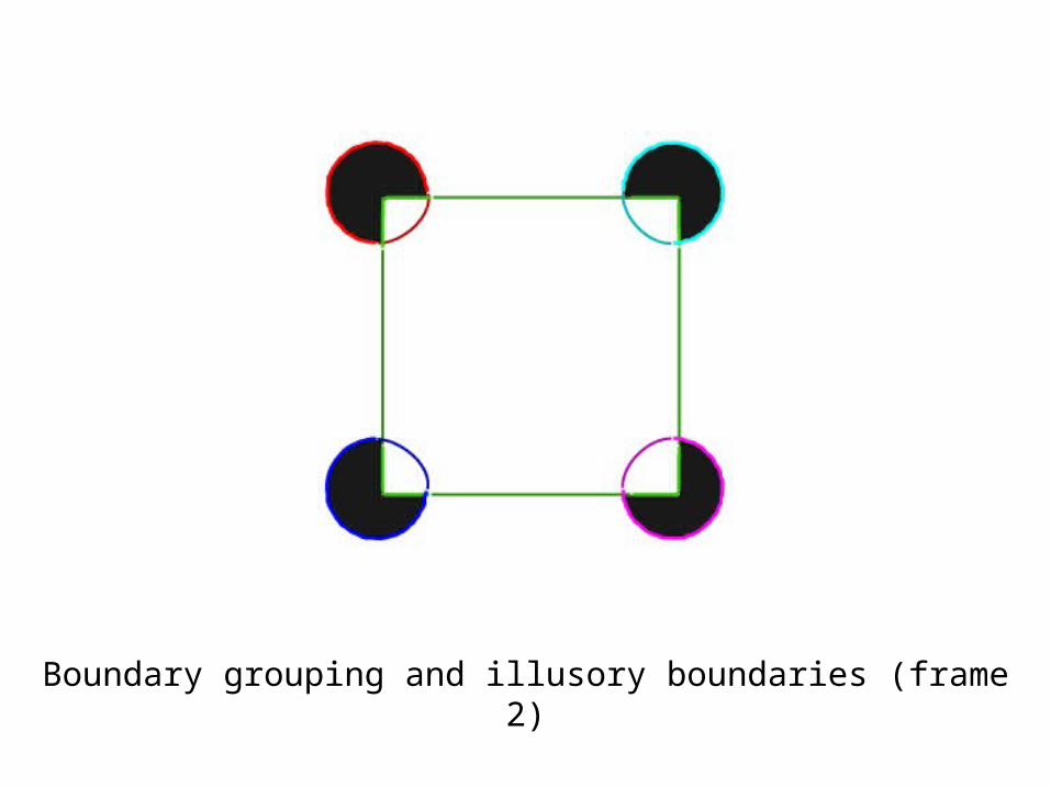
Boundary grouping and illusory boundaries (frame 2)

Dancer
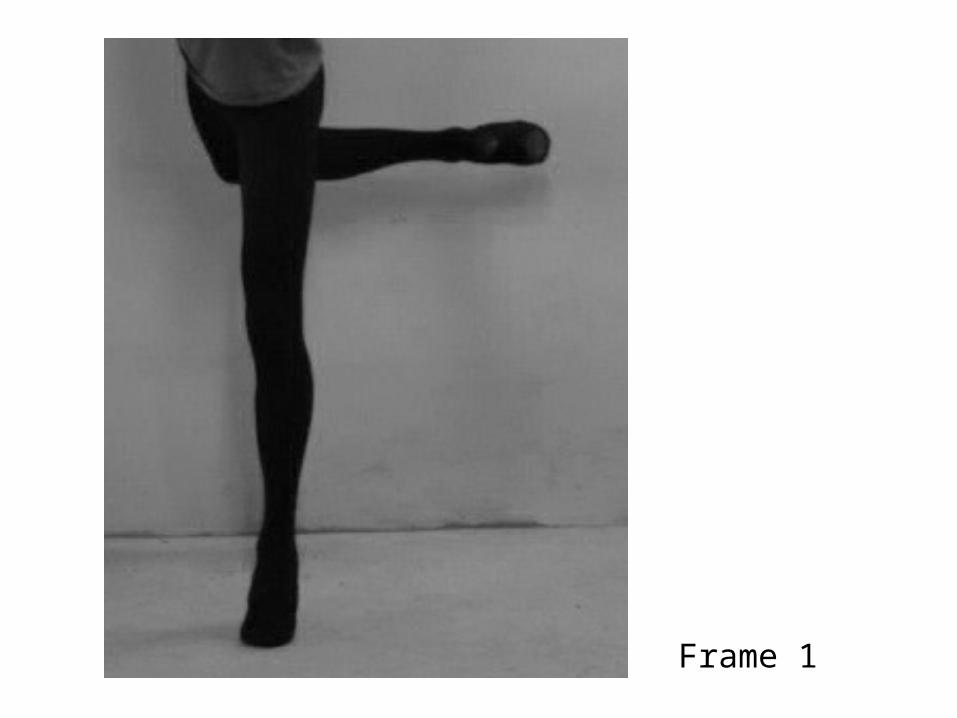
Frame 1
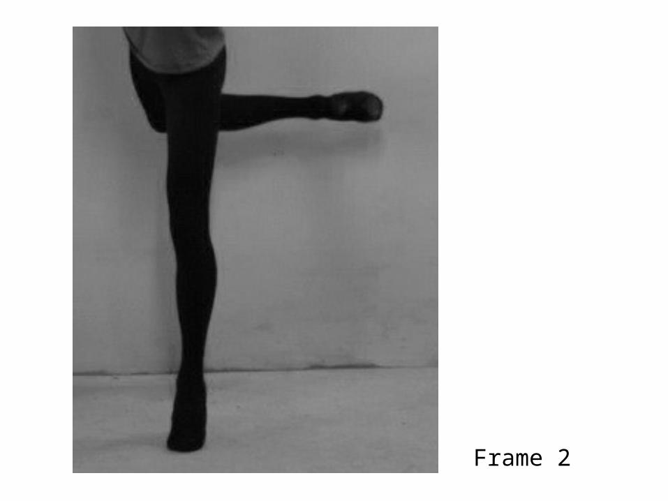
Frame 2
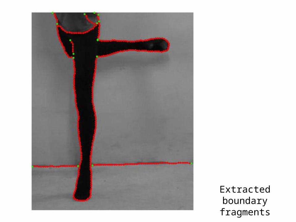
Extracted boundary fragments
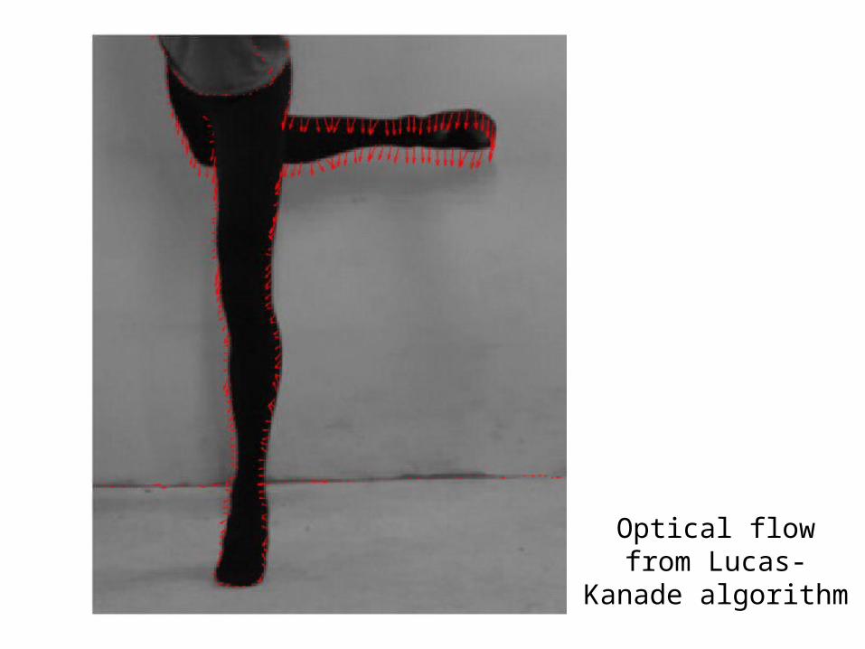
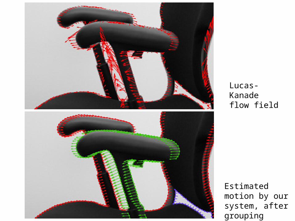
Optical flow from Lucas-Kanade
algorithm
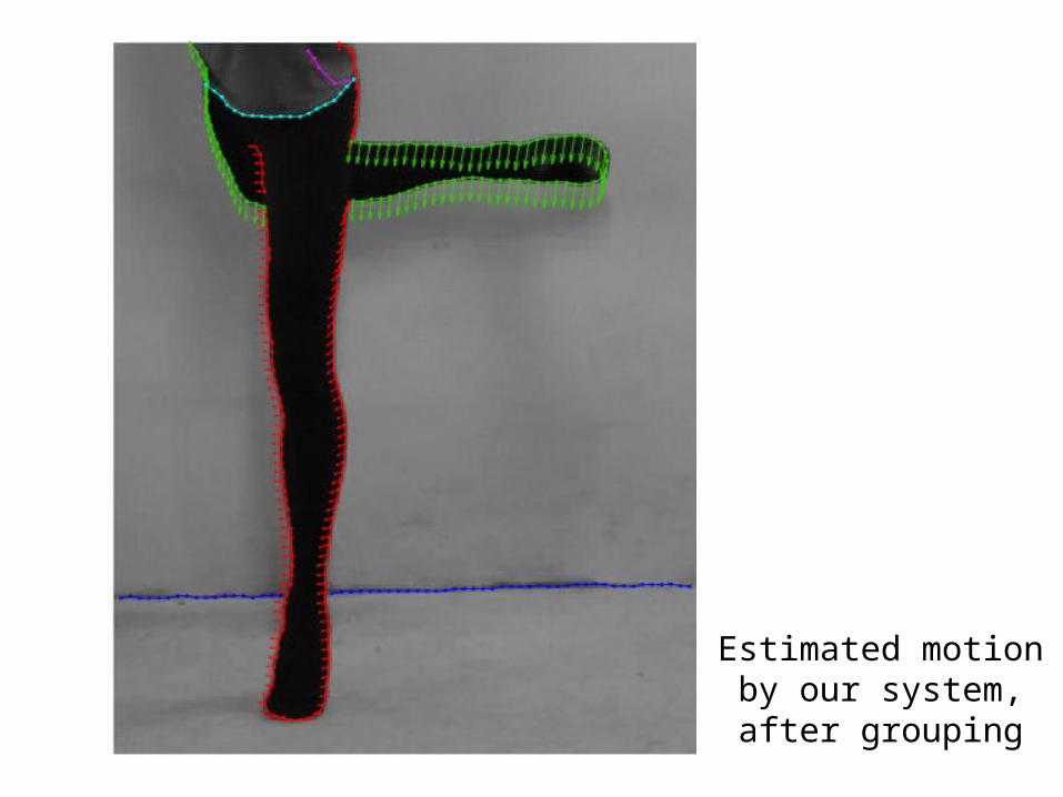
Estimated motion by our system, after
grouping
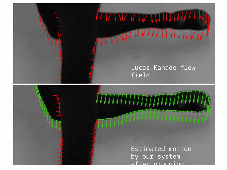
Lucas-Kanade flow field
Estimated motion by our system, after grouping
Boundary grouping and illusory boundaries
(frame 1)
Boundary grouping and illusory boundaries
(frame 2)

Rotating Chair

Frame 1
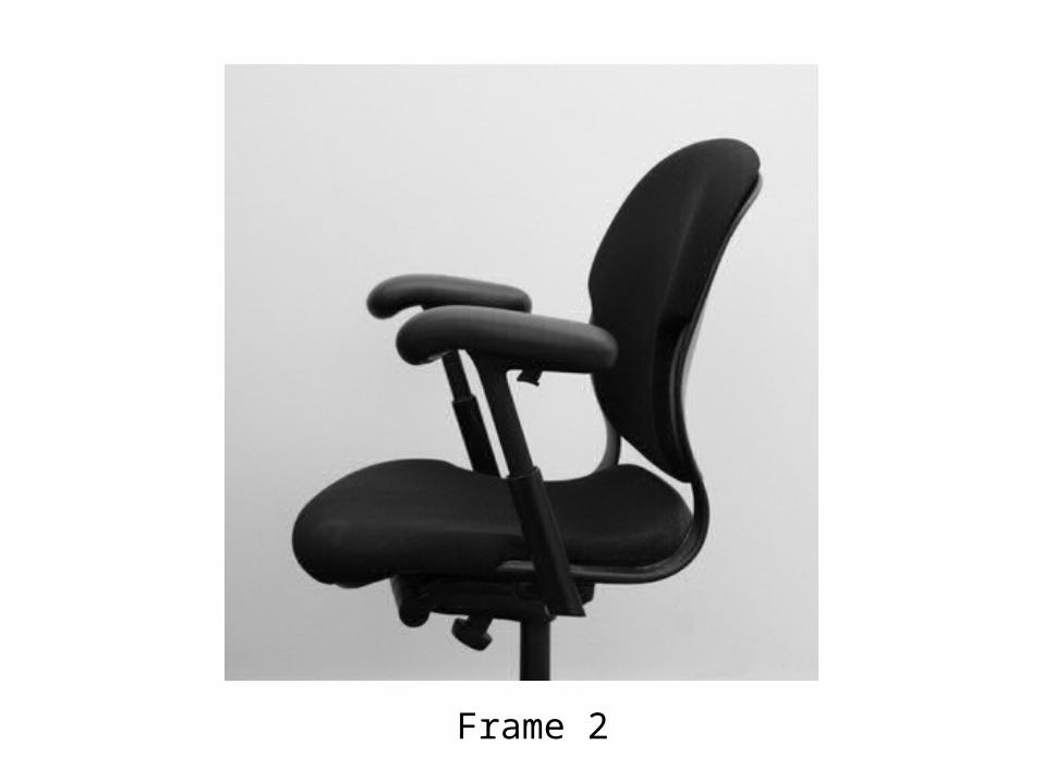
Frame 2
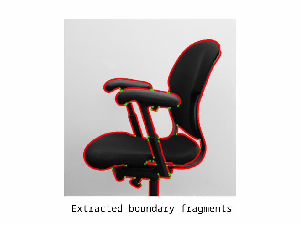
Extracted boundary fragments
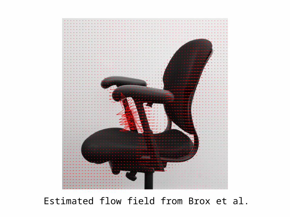
Estimated flow field from Brox et al.
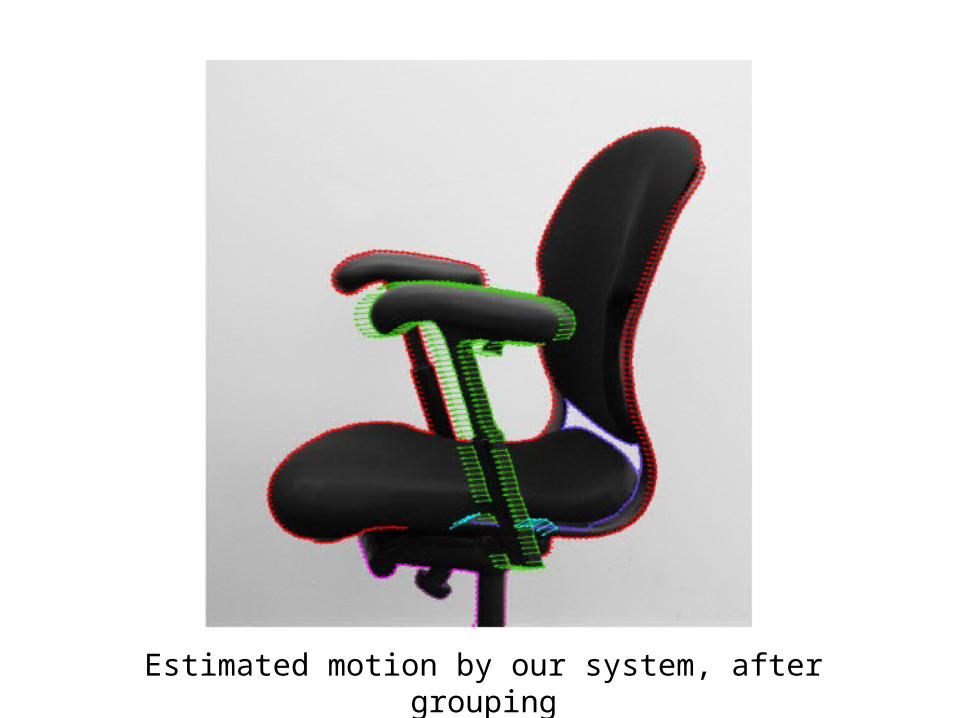
Estimated motion by our system, after grouping
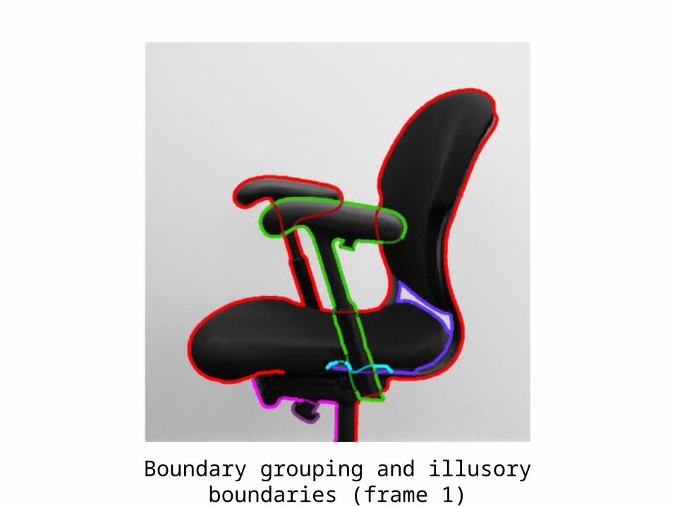
Boundary grouping and illusory boundaries (frame 1)
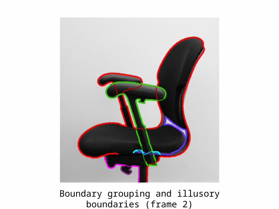
Boundary grouping and illusory boundaries (frame 2)
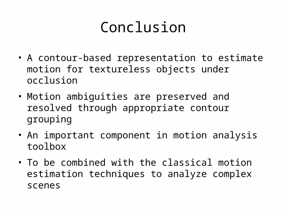
Conclusion
• A contour-based representation to estimate motion for textureless objects under occlusion
• Motion ambiguities are preserved and resolved through appropriate contour grouping
• An important component in motion analysis toolbox
• To be combined with the classical motion estimation techniques to analyze complex scenes
Thanks!
Analysis of Contour Motions
Ce Liu William T. Freeman Edward H. Adelson
Computer Science and Artificial Intelligence LaboratoryMassachusetts Institute of Technology
http://people.csail.mit.edu/celiu/contourmotions/

Backup Slides
1b2b
3b4b
Why bidirectional proposal in sampling?

Why bidirectional proposal in sampling?
1b2b
3b4b
b1b2: 0.39
b1b3: 0.01
b1b4: 0.60
Normalized affinity metrics
b4b1: 0.20
b4b2: 0.05
b4b3: 0.85
b2b1: 0.50
b2b3: 0.45
b2b4: 0.05
b3b1: 0.01
b3b2: 0.45
b3b4: 0.54
b1b2: 0.1750
b1b3: 0.0001
b1b4: 0.1200
Affinity metric of the switch variable (darker, thicker means larger affinity)
Bidirectional proposal
Why bidirectional proposal in sampling?
b1b2: 0.39
b1b3: 0.01
b1b4: 0.60
Normalized affinity metrics Bidirectional proposal(Normalized)
b4b1: 0.20
b4b2: 0.05
b4b3: 0.85
b2b1: 0.50
b2b3: 0.45
b2b4: 0.05
b3b1: 0.01
b3b2: 0.45
b3b4: 0.54
b1b2: 0.62
b1b3: 0.00
b1b4: 0.38
Bidirectional proposal of the switch variable (darker, thicker means larger affinity)
1b2b
3b4b
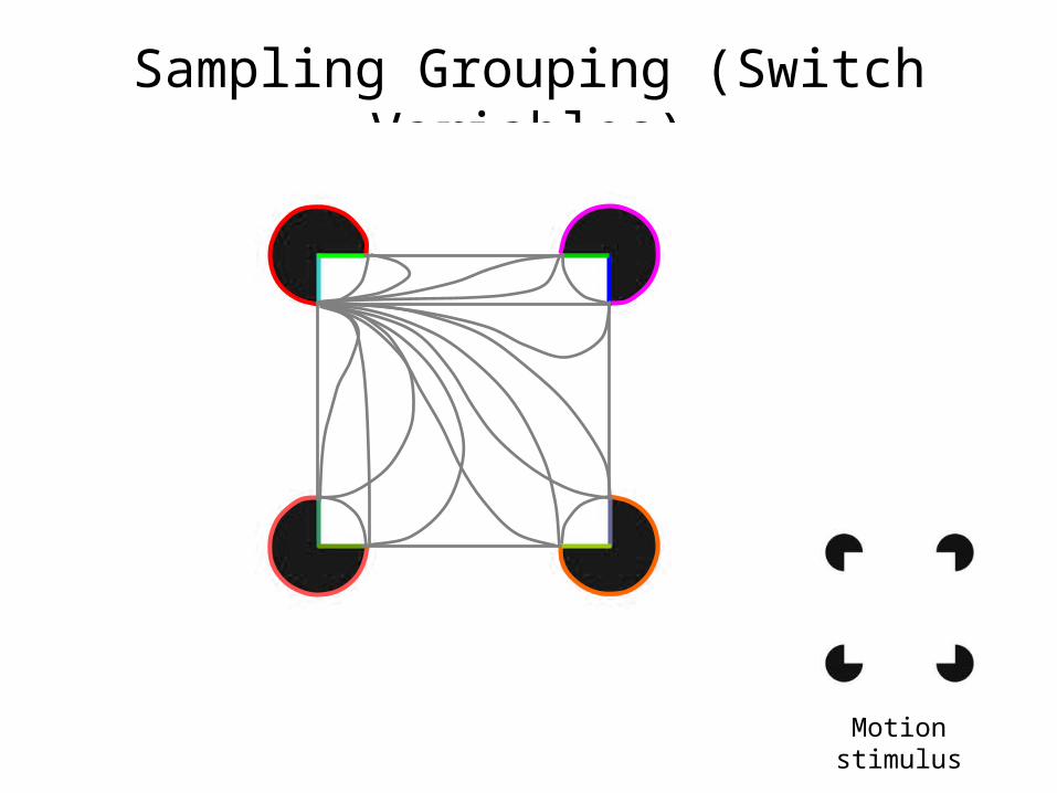
Sampling Grouping (Switch Variables)
Motion stimulus
Lucas-Kanade flow field
Estimated motion by our system, after grouping


![VALUE€¦ · Contour Drawing [Project One] Contour Drawing. Contour Line: In drawing, is an outline sketch of an object. [Project One]: Layered Contour Drawing The purpose of contour](https://img.pdfslide.us/doc/110x75/60363a1e4c7d150c4824002e/value-contour-drawing-project-one-contour-drawing-contour-line-in-drawing-is.jpg)