Embed Size (px)
Citation preview

ANALYSIS OF CONSIGNMENT CONTRACTSFOR SPARE PARTS INVENTORY SYSTEMS
a thesis
submitted to the department of industrial engineering
and the institute of engineering and science
of bilkent university
in partial fulfillment of the requirements
for the degree of
master of science
By
Cagrı Latifoglu
August, 2006

I certify that I have read this thesis and that in my opinion it is fully adequate,
in scope and in quality, as a thesis for the degree of Master of Science.
Assist. Prof. Alper Sen (Advisor)
I certify that I have read this thesis and that in my opinion it is fully adequate,
in scope and in quality, as a thesis for the degree of Master of Science.
Assist. Prof. Osman Alp
I certify that I have read this thesis and that in my opinion it is fully adequate,
in scope and in quality, as a thesis for the degree of Master of Science.
Assist. Prof. Yavuz Gunalay
Approved for the Institute of Engineering and Science:
Prof. Dr. Mehmet B. BarayDirector of the Institute
ii

ABSTRACT
ANALYSIS OF CONSIGNMENT CONTRACTS FORSPARE PARTS INVENTORY SYSTEMS
Cagrı Latifoglu
M.S. in Industrial Engineering
Supervisor: Assist. Prof. Alper Sen
August, 2006
We study a Vendor Managed Inventory (VMI) partnership between a manufacturer
and a retailer. More specifically, we consider a consignment contract, under which
the manufacturer assumes the ownership of the inventory in retailer’s premises until
the goods are sold, the retailer pays an annual fee to the manufacturer and the
manufacturer pays the retailer backorder penalties. The main motivation of this
research is our experience with a capital equipment manufacturer that manages the
spare parts (for its systems) inventory of its customers in their stock rooms. We
consider three factors that may potentially improve the supply chain efficiency un-
der such a partnership: i-) reduction in inventory ownership costs (per unit holding
cost) ii-) reduction in replenishment lead time and iii-) joint replenishment of multi-
ple retailer installations. We consider two cases. In the first case, there are no setup
costs; the retailer (before the contract) and the manufacturer (after the contract)
both manage the stock following an (S − 1, S) policy. In the second case, there are
setup costs; the retailer manages its inventories independently following an (r,Q)
policy before the contract, and the manufacturer manages inventories of multiple
retailer installations jointly following a (Q,S) policy. Through an extensive numer-
ical study, we investigate the impact of the physical improvements above and the
backorder penalties charged by the retailer on the total cost and the efficiency of
the supply chain.
Keywords: Inventory Models, Vendor Managed Inventory, Joint Replenishment
Problem, Supply Chain Contracts, Consignment Contracts.
iii

OZET
YEDEK PARCA ENVANTER SISTEMLERINDEKONSIMENTO KONTRATLARI
Cagrı Latifoglu
Endustri Muhendisligi, Yuksek Lisans
Tez Yoneticisi: Yrd. Doc. Dr. Alper Sen
Agustos, 2006
Bu tez calısmasında, bir imalatcı ile perakendeci arasındaki Tedarikci Yonetimli
Envanter anlasması incelenmistir. Ozellikle inceledigimiz konsimento anlasmasında,
perakendecinin tesislerindeki envanterin maliyet ve sorumlulugu yıllık bir ucret
karsılıgında imalatcıya gecmekte, imalatcı da yok satmalardan oturu perakendecinin
gorebilecegi zararları karsılamayı garanti etmektedir. Boyle bir ortaklıkta, tedarik
zinciri performansını iyilestirebilecek uc faktor incelenmektedir: i-) envanter
sahiplenme maliyetlerindeki azalma ii-) teslimat surelerindeki azalma iii-) birden
fazla perakende noktasının siparislerinin ortak verilebilmesi. Bunun icin iki du-
rum incelenmektedir. Ilk durumda, siparis vermenin sabit maliyeti yoktur. Bu
yuzden, hem anlasma oncesinde hem de anlasma sonrasında envanter yonetimi icin
(S − 1, S) politikası kullanılmaktadır. Ikinci durumda ise siparis vermenin sabit bir
maliyeti vardır. Bu yuzden, anlasma oncesinde, perakendeci noktalarındaki envan-
terler, perakendeciler tarafından birbirlerinden bagımsız olarak, (r,Q) politikasına
gore, anlasma sonrasında ise imalatcı tarafından ortak olarak (Q,S) politikasına
gore yonetilir. Kapsamlı bir sayısal analiz ile, bu iyilestirmelerin ve imalatcının per-
akendeciye yok satmalardan dolayı odedigi cezaların tedarik zinciri maliyetleri ve
etkinligi uzerindeki etkileri incelenmektedir.
Anahtar sozcukler : Envanter Sistemleri, Tedarikci Yonetimli Envanter, Toplu
Siparis Politikaları, Tedarik Zinciri Kontratları, Konsimento Kontratları.
iv

Acknowledgement
I would like to express my most sincere gratitude to my advisor and mentor, Asst.
Prof. Alper Sen for all the trust, patience and endurance that he showed during my
graduate study. Without his guidance, understanding and contribution, I would not
be able to make it to where I am now. I hope I can live up to his expectations from
me.
I am also indebted to Assist. Prof. Osman Alp and Assist. Prof. Yavuz Gunalay
for excepting to read and review this thesis and for their invaluable suggestions.
I would like to express my deepest gratitude to Prof. Selim Akturk and Prof.
Mustafa C. Pınar for their wise suggestions and fatherly approach. I also would like
to thank to all faculty members of our department for devoting their time, effort,
understanding and friendship.
I want to thank Zumbul Bulut for always being there for me. I also want to
express my gratitude to Aysegul Altın for being a good friend.
I am grateful to my dear friends Evren Korpeoglu, Fazıl Pac, Ahmet Camcı,
Onder Bulut, Safa Erenay, Mehmet Mustafa Tanrıkulu, N. Cagdas Buyukkaramıklı
and Muzaffer Mısırcı for their understanding and sincere friendship. I also express
thanks to all Kaytarıkcılar for their help and morale support.
Last but not the least, I wish to express my gratitude to my family. They are
the most valuable for me.
v

Contents
1 Introduction 1
2 Literature Survey 10
3 Models 22
3.1 Base Stock Policy . . . . . . . . . . . . . . . . . . . . . . . . . . . . . 23
3.2 (r,Q) Policy . . . . . . . . . . . . . . . . . . . . . . . . . . . . . . . . 25
3.3 (Q,S) Policy . . . . . . . . . . . . . . . . . . . . . . . . . . . . . . . 27
3.4 Contracts . . . . . . . . . . . . . . . . . . . . . . . . . . . . . . . . . 30
3.4.1 Without Setup Costs . . . . . . . . . . . . . . . . . . . . . . . 33
3.4.2 With Setup Costs . . . . . . . . . . . . . . . . . . . . . . . . . 35
4 Contracts Without Setup Costs 39
4.1 Physical Improvement Under Centralized Control . . . . . . . . . . . 40
4.1.1 Leadtime Reduction . . . . . . . . . . . . . . . . . . . . . . . 41
4.1.2 Holding Cost Reduction . . . . . . . . . . . . . . . . . . . . . 45
vi

CONTENTS vii
4.2 Decentralized Control . . . . . . . . . . . . . . . . . . . . . . . . . . . 50
4.2.1 Decentralized Control with Leadtime Reduction . . . . . . . . 51
4.2.2 Decentralized Control with Holding Cost Reduction . . . . . . 56
5 Contracts with Setup Costs 61
5.1 Effect of Pure JRP . . . . . . . . . . . . . . . . . . . . . . . . . . . . 62
5.2 Physical Improvement Under Centralized Control . . . . . . . . . . . 73
5.2.1 Contracts With Setup Cost - Leadtime Improvement . . . . . 75
5.2.2 Contracts With Setup Cost - Holding cost improvement . . . . 79
5.3 Decentralized Control . . . . . . . . . . . . . . . . . . . . . . . . . . . 83
6 Conclusion 92

List of Figures
3.1 Supply Chain Parameters Before and After Contract . . . . . . . . . 32
5.1 Pure JRP Savings - π′m = 0, hm = 6, Lm = 2 . . . . . . . . . . . . . . 63
5.2 Pure JRP Savings - πm = 0, hm = 6, Lm = 2 . . . . . . . . . . . . . . 64
5.3 Pure JRP Savings - πm = 50, π′m = 0, Lm = 2 . . . . . . . . . . . . . 65
5.4 Pure JRP Savings - πm = 0, π′m = 50, Lm = 2 . . . . . . . . . . . . . 67
5.5 Pure JRP Savings - πm = 50, π′m = 0, h=6 . . . . . . . . . . . . . . . 69
5.6 Pure JRP Savings - πm = 0, π′m = 50, h=6 . . . . . . . . . . . . . . . 71
5.7 Pure JRP Savings - πm = 50, π′m = 0, hm = 6, Lm = 2 . . . . . . . . . 72
5.8 Pure JRP Savings - πm = 0, π′m = 50, hm = 6, Lm = 2 . . . . . . . . . 73
5.9 Contracts with Setup - Leadtime Improvement, πm = 50, π′m = 0 . . . 75
5.10 Contracts with Setup - Leadtime Improvement, πm = 100, π′m = 0 . . 77
5.11 Contracts with Setup - Leadtime Improvement, πm = 0, π′m = 50 . . . 78
5.12 Contracts with Setup - Leadtime Improvement, πm = 0, π′m = 100 . . 79
5.13 Contracts with Setup - Holding Cost Improvement, πm = 50, π′m = 0 80
viii

LIST OF FIGURES ix
5.14 Contracts with Setup - Holding Cost Improvement, πm = 100, π′m = 0 81
5.15 Contracts with Setup - Holding Cost Improvement, πm = 0, π′m = 50 82
5.16 Contracts with Setup - Holding Cost Improvement, πm = 0, π′m = 100 83
5.17 Contracts with Setup, Decentralized Control, πm = 0, π′m = 10 : 150,
Case: 1, 2, 3 . . . . . . . . . . . . . . . . . . . . . . . . . . . . . . . . 86
5.18 Contracts with Setup, Decentralized Control, πm = 0, π′m = 10 : 150,
Case 1 Costs . . . . . . . . . . . . . . . . . . . . . . . . . . . . . . . . 86
5.19 Contracts with Setup, Decentralized Control, πm = 0, π′m = 25 : 75,
Case:4, 5, 6 . . . . . . . . . . . . . . . . . . . . . . . . . . . . . . . . 87
5.20 Contracts with Setup, Decentralized Control, πm = 0, π′m = 25 : 75,
Case 3 Costs . . . . . . . . . . . . . . . . . . . . . . . . . . . . . . . . 88
5.21 Contracts with Setup, Decentralized Control,πm = 25 : 75, π′m = 0,
Case:7, 8, 9 . . . . . . . . . . . . . . . . . . . . . . . . . . . . . . . . 89
5.22 Contracts with Setup, Decentralized Control, πm = 25 : 75, π′m = 0,
Case 7 Costs . . . . . . . . . . . . . . . . . . . . . . . . . . . . . . . . 89
5.23 Contracts with Setup, Decentralized Control, πm = 25 : 75, π′m = 0,
Case:10, 11, 12 . . . . . . . . . . . . . . . . . . . . . . . . . . . . . . 90
5.24 Contracts with Setup, Decentralized Control, πm = 25 : 75, π′m = 0,
Case 10 Costs . . . . . . . . . . . . . . . . . . . . . . . . . . . . . . . 91

List of Tables
4.1 Physical Improvement Base Case Parameters . . . . . . . . . . . . . . 39
4.2 Physical Improvement Base Case Optimal Sr and Cost Components . 40
4.3 Base Case 1 Percentage Savings - Leadtime Reduction . . . . . . . . 41
4.4 Base Case 1 Annual Payment Bounds - Leadtime Reduction . . . . . 42
4.5 Base Case 2 Percentage Savings - Leadtime Reduction . . . . . . . . 43
4.6 Base Case 3 Percentage Savings - Leadtime Reduction . . . . . . . . 44
4.7 Base Case 4 Percentage Savings, Leadtime Reduction . . . . . . . . . 44
4.8 Base Case 1 Percentage Savings - Holding Cost Reduction . . . . . . 45
4.9 Base Case 1 Annual Payment Bounds - Holding Cost Reduction . . . 46
4.10 Base Case 2 Percentage Savings - Holding Cost Reduction . . . . . . 47
4.11 Base Case 3 Percentage Savings - Holding Cost Reduction . . . . . . 48
4.12 Base Case 4 Percentage Savings, Holding Cost Reduction . . . . . . . 49
4.13 Decentralized Channel - Base Case Parameters . . . . . . . . . . . . . 50
4.14 Decentralized Channel - Base Case Optimal Sr and Cost Components 51
4.15 Base Case 1 Percentage Savings, Lm = 1.5, π′m changes . . . . . . . . 51
x

LIST OF TABLES xi
4.16 Base Case 2 Percentage Savings, Lm = 1.5, π′m changes . . . . . . . . 52
4.17 Base Case 3 Percentage Savings, Lm = 1.5, πm changes . . . . . . . . 53
4.18 Base Case 4 Percentage Savings, Lm = 1.5, πm changes . . . . . . . . 54
4.19 Base Case 1 Percentage Savings, hm = 4, π′m changes . . . . . . . . . 56
4.20 Base Case 2 Percentage Savings, hm = 4, π′m changes . . . . . . . . . 57
4.21 Base Case 3 Percentage Savings, hm = 4, πm changes . . . . . . . . . 58
4.22 Base Case 4 Percentage Savings, hm = 4, πm changes . . . . . . . . . 59
5.1 Pure JRP Savings - π′m = 0, hm = 6, Lm = 2 . . . . . . . . . . . . . . 62
5.2 Pure JRP Savings - πm = 0, hm = 6, Lm = 2 . . . . . . . . . . . . . . 64
5.3 Pure JRP Savings - πm = 50, π′m = 0, Lm = 2 . . . . . . . . . . . . . 65
5.4 Pure JRP Savings - πm = 0, π′m = 50, Lm = 2 . . . . . . . . . . . . . 67
5.5 Pure JRP Savings - πm = 50, π′m = 0, h=6 . . . . . . . . . . . . . . . 69
5.6 Pure JRP Savings - πm = 0, π′m = 50, h=6 . . . . . . . . . . . . . . . 70
5.7 Pure JRP Savings - πm = 50, π′m = 0, hm = 6, Lm = 2 . . . . . . . . . 71
5.8 Pure JRP Savings - πm = 0, π′m = 50, hm = 6, Lm = 2 . . . . . . . . . 72
5.9 Contracts with Setup - Base Case Parameter Summary . . . . . . . . 74
5.10 Contracts with Setup - Base Case Solution Summary . . . . . . . . . 74
5.11 Contracts with Setup - Leadtime Improvement, πm = 50, π′m = 0,
Case:1,2,3 . . . . . . . . . . . . . . . . . . . . . . . . . . . . . . . . . 75
5.12 Contracts with Setup - Leadtime Improvement, πm = 100, π′m = 0 . . 76

LIST OF TABLES xii
5.13 Contracts with Setup - Leadtime Improvement, πm = 0, πm′ = 50 . . 77
5.14 Contracts with Setup - Leadtime Improvement, πm = 0, π′m = 100 . . 78
5.15 Contracts with Setup - Holding Cost Improvement, πm = 50, π′m = 0 79
5.16 Contracts with Setup - Holding Cost Improvement, πm = 100, π′m = 0 80
5.17 Contracts with Setup - Holding Cost Improvement, πm = 0, π′m = 50 81
5.18 Contracts with Setup - Holding Cost Improvement, πm = 0, π′m = 100 82
5.19 Contracts with Setup, Decentralized Control - Base Case Parameter
Summary . . . . . . . . . . . . . . . . . . . . . . . . . . . . . . . . . 84
5.20 Contracts with Setup, Decentralized Control - Base Case Solution
Summary . . . . . . . . . . . . . . . . . . . . . . . . . . . . . . . . . 85
5.21 Contracts with Setup, Decentralized Control, πm = 0, π′m = 10 : 150,
Case: 1, 2, 3 . . . . . . . . . . . . . . . . . . . . . . . . . . . . . . . . 85
5.22 Contracts with Setup, Decentralized Control, πm = 0, π′m = 25 : 75,
Case:4, 5, 6 . . . . . . . . . . . . . . . . . . . . . . . . . . . . . . . . 87
5.23 Contracts with Setup, Decentralized Control, πm = 25 : 75, π′m = 0,
Case:7, 8, 9 . . . . . . . . . . . . . . . . . . . . . . . . . . . . . . . . 88
5.24 Contracts with Setup, Decentralized Control, πm = 25 : 75, π′m = 0,
Case:10, 11, 12 . . . . . . . . . . . . . . . . . . . . . . . . . . . . . . 90

Chapter 1
Introduction
We study full service Vendor Managed Inventory (VMI) contracts for spare parts.
These contracts are consignment agreements, between the manufacturer and its cus-
tomers, where all decisions and services related to spare parts are assumed by the
manufacturer in return for an annual fee that is paid by the customers. Ownership of
the material is also assumed by the manufacturer until consumption takes place. We
also investigate the Joint Replenishment Problem (JRP) for such a setting where we
compare independent and joint replenishment of various installations of customers.
Full service VMI contracts or consignment contracts have various potential benefits.
Operational benefits of consignment contracts include reduction in cost of owning
inventory, reduction in replenishment leadtime and the ability to jointly replenish
multiple locations and items. Strategically, the manufacturer increases its market
share and strengthens its relationships with customers by establishing such con-
tracts. On the other hand customers receive high quality service for highly complex
material while spending their effort and time on their own operations, instead of
inventory and logistics management of spare parts.
Full service was defined by Stremersch [49] as comprehensive bundles of prod-
ucts and/or services that fully satisfy the needs and wants of a customer. The main
driver of the full service contracts is the change in the products and the retailers.
Short product life-cycles and time-to-market, forces companies to design, produce
1

CHAPTER 1. INTRODUCTION 2
and market rapidly. Along with consignment, full service contracts provide the re-
quired flexibility and agility for such markets. Those contracts are usually structured
considering the nature of the business and ordering procedures, receipt and issuance
procedures, documentation requirements, data management requirements, place of
delivery, time limits and service levels, financing and payments, qualifications and
quality requirements. But the comprehensive nature of the contracts makes it diffi-
cult to assess and measure the performance of contracts. Because of that reason, the
performance evaluation mechanism are also sophisticated. Various criteria such as
depth of contract, scope of the contract, type of installations to maintain, degree of
subcontracting, detail of information, supplier reputation, influence on performance,
influence on total costs and influence on maintenance costs are used to evaluate and
asses the performance of full-service contracts.
The main motivation of this research is due to our experience from a leading
capital equipment manufacturer which has such a relationship with its customers.
The manufacturer produces systems that perform most of the core operations in high
technology material production. The customers of the company are electronics man-
ufacturers which either use these high technology materials in their own products
or sell them to other companies downstream. The capital equipment manufacturer
owns research, development and manufacturing facilities in various locations such
as United States, Europe and Far East which provide complex and expensive sys-
tems to world’s leading electronic equipment companies. The manufacturer is at the
topmost place in the related supply chain.
In our setting, the manufacturer provides spare parts of capital equipment to its
customers. Capital equipments are very expensive and important investments. Cost
of idle capacity due to equipment failures or service parts inventory shortages for
customers is very high. For this reason the manufacturer set up a large spare parts
network. This network consists of more than 70 locations across the globe, which
includes 3 company owned continental distribution centers (in Europe, North Amer-
ica and Asia) and depots. Company also owns stock rooms as a part of spare parts
network, in facilities of customers which has an agreement with the manufacturer.
The distribution network is mainly responsible for procuring and distributing spare
parts to depots, company owned stock rooms and customers. The depots are located

CHAPTER 1. INTRODUCTION 3
such that they can provide 4-hour service to any unforeseen request. Continental
distribution centers also serve orders from specific customers, orders that can not
be satisfied by local depots and orders that are related to scheduled maintenance
activities. Customer orders go through an order fulfillment system which searches
for available inventory in different locations according to order sequence specific to
each customer. The complexity of this network is further increased by more than
50,000 consumable and non-consumable parts and varying service level requirements
of the customers.
Managing this immense supply chain requires a great coordination in transporta-
tion and inventory decisions. Full service contracts helps both manufacturer and its
customers in coordination. We defined the operational and strategic benefits of full
service contracts and those provide the required incentives to parties to participate
in the agreement. There are two key observations about our supply setting: First,
the manufacturer has a lower per unit holding cost than its customer since there
is no additional profit margin on price of material that is incurred by customer.
Also there are technical reasons, such as better preservation conditions provided for
sensitive material. Second, order processing times are reduced significantly and this
is enhanced with clarity of demand due to implementation of information sharing
and online ordering technologies. For example, the stock rooms have a direct access
to the manufacturer’s ERP system under the consignment contracts.
In this research we focus on coordination issues of this complex supply chain
with consignment contracts. Contracts may have different purposes such as shar-
ing the risks arising from various sources of uncertainty, coordinating supply chain
through eliminating inefficiencies (e.g. double marginalization), defining benefits
and penalties of cooperative and non-cooperative behavior, building long-term rela-
tionships and explicitly clarifying terms of relationships. Also there may be different
classification schemes for contracts such as specification of decision rights, pricing,
minimum purchase commitments, quantity flexibility, buy back or returns policies,
allocation rules, leadtimes and quality.
We consider a setting in which inventory is owned and all replenishment deci-
sions are made by the manufacturer, and the customers pay an annual fee for this

CHAPTER 1. INTRODUCTION 4
service. So the contract that we are considering is a consignment contract. Con-
signment may be defined as the process of a supplier placing goods at a customer
location without being paid until the goods are used or sold. In practice, the man-
ufacturer owns stock rooms in facilities of those customers where spare parts are
kept. The key point that should be carefully handled in consignment contracts is
the level of consigned inventory. A customer would prefer to hold a large amount
of consigned inventory, since she does not have any financial obligation. The sup-
plier, however, must determine the level at which it can provide goods profitably.
Below we briefly review vendor managed inventory systems, supply chain contracts,
consignment contracts and joint replenishment / inventory systems.
For lack of information, inventory is used as a proxy. In the absence of well
timed and precise demand information, the lack of information is compensated with
material stacks. The supplier will see batched orders from the buyer, which may
not represent “true” end-customer demand. False demand signals and lack of infor-
mation sharing lead to “Bullwhip Effect” which can ripple upwards in supply chain
raising costs and creating disruptions. As demand information flows upwards in
real time, production is more aligned with demand and supply chain performance
is increased through decreasing inventories and increasing service levels. In order
to achieve increased supply chain performance, VMI concept focuses on control of
decision maker and ownership rights. The decision maker controls the timing and
size of orders to provide benefits. Under VMI, the vendor has a certain level of
responsibility of inventory decisions of customers with whom she has such a VMI
partnership. In the simplest form, VMI is the practice that vendor assumes the task
of generating purchase orders to replenish a customer’s inventory. VMI partnerships
may arise at any point of supply chain. For example, it can be between manufac-
turer and wholesale distributor, wholesale distributor and retailer, manufacturer
and end-customer. In a VMI partnership there are varying degrees of collabora-
tion. In the most primitive type, vendor and buyer share data and jointly develop
forecasts and/or production schedules amongst supply chain partners. In a more
advanced form of VMI partnership, activity and costs of managing inventory are
transferred to supplying organization and this type of partnership is closer to our
model. In the most advanced form, constraints and goals of customer and supplier

CHAPTER 1. INTRODUCTION 5
are integrated under the guidance of market intelligence provided by the supplier to
achieve better supply chain performance. Hausman [30] introduced the “Supplier
Managed Availability” concept, which states that inventory at downstream site is
not an aim itself but just an enabler of sales or production activity. There are
other methods to provide “availability” other than stocking inventory such as using
faster modes of transportation and producing faster. Supplier managed availabil-
ity concept is similar to VMI in spirit. Under VMI, service level to end customer,
sales, return on assets increases while routine replenishment activities and fulfillment
costs decreases at the buyer level. Similar improvements are experienced at supplier
while smoother demand patterns are realized. Setting, reviewing and maintaining
performance goals, minimizing supply chain transactions through SKU’s, ensuring
data accuracy, utilizing market intelligence to augment automated replenishment
decisions, conducting performance reviews and using the metrics to find costs and
inefficiencies, then eliminating them cooperatively are keys for successful VMI im-
plementation.
As shorter product life cycles squeezed profit margins, manufacturers are forced
to focus on cost-of-ownership and production-worthiness. As reviewed by Arnold [2]
in a typical chip production facility, for every dollar worth of materials that stays
in stock for a year, 35 cents are accounted for inventory expenses. Another article
by Mahendroo [34] reviews the partnership between world’s leading semiconductor
equipment manufacturing company Applied Materials and its customer, LSI. This
partnership is an exemplary one in VMI context. Applied Material (AMAT) pro-
vides a service called Total Support Package to LSI to accelerate transition to its
systems. As stated in AMAT’s annual report [1] Total Support Package covers all
maintenance service and spare parts needed for Applied Material products, allowing
LSI to quickly bring a system to production readiness without requiring additional
investment in parts inventory build-up or adding/training new technical service sup-
port personnel. By monitoring and optimizing system performance on an on-going
basis, this agreement reduced equipment operating costs, transaction costs by elim-
ination of invoicing and accounts reconciliation, delivery costs through shipment
consolidation, number of in house technicians and service part number duplication

CHAPTER 1. INTRODUCTION 6
and administrative overhead costs while improving inventory standardization, man-
agement of inventories and service levels. Mahendroo [34] states that 15-30% lower
cost and 200% tool utilization are obtained through this partnership.
A case study by Corbett et al. [20], presents the VMI relationship between Pel-
ton International and its two customers: Perdielli Milan and Basco PLC. Pelton
International is a multinational chemical firm. In that agreement, Pelton suggested
consignment stocks as an incentive for standard keeping unit (SKU) rationalization
to Perdielli and Basco. With that agreement Pelton international radically improved
the relationship with Perdielli, increased standardization, reduced safety stocks and
scheduling complexity, increased rationalization and reduced rush orders. On the
customer side, Basco PLC exploited the benefits of consignment stock while ex-
periencing more reliable deliveries related to integrated planning and forecasting.
Perdielli Milan also reaped the benefits of consignment stock while reducing staff
in purchasing department and got business experience in supply chain improvement
which they began instituting with other suppliers. The relationship between Boeing,
Rockwell Collins and Goodrich is another example for full service consignment that
can be found in airframe maintenance sector [11]. The parts that are needed for
airframe production is stored at customer sites or more commonly at Boeing ware-
houses in proximity to customer installations where logistics and transportation are
handled by Boeing. The shift from traditional original equipment manufacturers to
total service providers can be seen in this partnership.
Pan Pro LLC is a provider of advanced supply chain software solutions. In their
web primer [36] they note the extensive information sharing and coordination re-
quirement of VMI implementations. To achieve that, companies utilize technologies
such as POS, EDI, XML, FTP and other reliable information sharing technologies.
The level to which information will be shared and utilized are controlled by the con-
tracts since information sharing certainly creates a strategic advantage which may
be exploited by the partners in those contracts. It shall be ensured that both parties
have strong incentives and commitment. VMI implementations will not be success-
ful if required incentive, technical base and logistic infrastructure are not provided.
Supply chains, which consist of multiple players with possibly conflicting objectives
connected by flow of information, goods and money, often suffer from the quandary

CHAPTER 1. INTRODUCTION 7
of conflicting performance measures. For example a low level of inventory may be a
contradiction to high service level requirements. Contracts shall insure that parties
will behave according to supply chain goals instead of their own goals. Obviously
the nature of the products and demand affect how VMI will be implemented. For
example in retail sector, inventory just enables the sales but as in our setting (cap-
ital equipment spare parts which consist of very expensive and critical material)
inventory prevents unexpected and expensive down times and capacity losses. So
the nature of the setting where VMI will be applied, shall be carefully integrated
and contracts should be structured using this knowledge.
Other than participating to a consignment contract, the capital equipment man-
ufacturer that we mentioned earlier also plans to jointly replenish the various loca-
tions in spare parts network. In existing practice, orders are treated separately, even
if they come from various installations of the same customer. Under consignment
contracts, the inventory control and decision rights of those locations are centralized
under the control of the manufacturer which will allow the utilization of joint replen-
ishment techniques. The Joint Replenishment Problem (JRP) has been a renowned
research topic since it is a common real-world problem. JRP is also relevant when
a group of items are purchased from the same supplier. The characteristics of the
spare parts network such as multi product service requirement of the customers
and existence of customers with multiple installations, are very similar to these two
occurrences. By utilizing different modes of transportation, adjusting the timing
and quantity of the replenishment, the manufacturer plans to exploit the benefits of
JRP.
Before moving further, we explain how leadtimes and holding costs are improved
under manufacturer control. As we mentioned before the spare parts that we are
considering are very sensitive and high technology material which require special
stocking environments and attention of expert personnel. The manufacturer has
more technical expertise on the creating and maintaining such environments since
she is the one who produces them. Also the manufacturer already has expert per-
sonnel for operating such environments. When retailer has to invest additional
time and effort providing those requirements when she controls such environments.
Therefore, we reflect this difference to costs in terms of holding costs. Also when

CHAPTER 1. INTRODUCTION 8
manufacturer assumes the control, information systems of the manufacturer and
the retailer are integrated. The stock rooms in retailer facilities are connected to
the manufacturer’s ERP software which provide continuous and precise monitoring.
Consequently order processing times and invoicing activities are reduced which in
turn reduces leadtimes. Other than that, the manufacturer utilizes different modes
of transportation to replenish retailer facilities jointly which makes it easier to ex-
ploit benefits of mass transportation.
By utilizing consignment contracts and joint replenishment, the manufacturer
aims to secure a market share by building strong relationships with its customers
through contracts. Obviously being the preferred supplier of the majority of the
customers in the market brings significant business advantages. Also with VMI
and JRP, the manufacturer will obtain crucial demand data rapidly with less noise
through integration of information systems which will in turn improve production
plans, supply better coordination in deliveries and decrease ordering transactions.
Obviously, the manufacturer wants to achieve short-term and long-term benefits
that we specified in a profitable manner. All arrangements that are required to
make VMI and JRP work, have costs significant costs, therefore this problem shall
be carefully studied. In customers’ perspective, in short term they will achieve in-
creased product availability and backorder subsidies. In long term customers focus
time and effort on their own operations rather than inventory management activities
in return for an annual fee. Again profitability is the key for customer participation.
When the whole supply chain is considered; elimination of incentive conflicts and
provision of savings, which will be allocated to participants to improve their stand-
ings through utilization of VMI and JRP, are required to coordinate the channel.
In this thesis, we first demonstrate the savings obtained from utilization of consign-
ment contracts. By using the manufacturer’s lower leadtime and holding cost, it
is possible to achieve a lower total supply chain cost. Then we consider JRP and
demonstrate that significant savings are possible by jointly replenishing multiple
retailer installations that are part of a consignment contract. In various scenarios
involving JRP and VMI, we investigate affect of various parameters such as holding
costs, leadtime, ordering costs and backorder costs on these savings. By using this

CHAPTER 1. INTRODUCTION 9
information, we search for the conditions (i.e. parameter ranges), under which par-
ties agree to partnership. Obviously parties need to be better off than their initial
standing to participate this contract. Finally we investigate how different allocation
methods affect the participation and profits of the parties. We shall note that, even
if one of the parties does not earn benefits from the contract, due to beforehand
mentioned strategic reasons, she may choose to participate to contract. But in this
research, we exclude that option.
The remainder of thesis is organized as follows. In Chapter 2, we provide a
review of the literature in VMI, supply chain contracts, inventory theory and joint
replenishment problem. In Chapter 3, we present the models for various inventory
policies that will be used in investigating affects of VMI and JRP. Using those mod-
els, we construct contract models and formulate savings. In Chapter 4, we present
our numerical results related to contracts without setup costs. We investigate supply
chain coordinating values of various contract parameters. We also present savings
achieved in supply chain through those contracts. In Chapter 5, we present the re-
sults of our numerical study related to contracts where there are setup costs. First
effect of pure JRP will be demonstrated. Secondly the joint effect of VMI and JRP
is demonstrated using comparison of (Q,S) policy and (r,Q) policy. In Chapter
6, we conclude the thesis giving an overall summary of what we have done, our
contribution to the existing literature and its practical implications.

Chapter 2
Literature Survey
Christopher [18] defines the supply chain as a network of organizations that are
involved with upstream and downstream linkages in different processes and activities
that produce value to the products or services. Persson [38] states the objectives of
supply chain management as a set of cardinal beliefs; coordination and integration
along the material flow, win-win relations and end customer focus. She also puts
forward that there is much empirical evidence of benefits achieved when supply
chain management is used effectively. For a long time the organizations in the
supply chain have seen themselves as independent entities. But to survive in today’s
competitive environment, supply chains are becoming more integrated. First units
of firms with similar functions become closer, then an internal integration occurs
within the company and after that external integration with suppliers and customers
occur. There are several concepts related to supply chain management and those
are summarized by Waters [58] as follows:
• Improving communications: Integrated and increased communication within the
supply chain with new technologies such as Electronic Data Interchange (EDI).
• Improving customer service: Increasing customer service levels while decreasing
the costs.
• Globalization: As communication around the globe is increasing, companies be-
come more international to survive in increasing competition and trade.
10
CHAPTER 2. LITERATURE SURVEY 11
• Reduced number of suppliers: Better and long term relationships are created
with a small number of suppliers.
• Concentration of ownership: Fewer players control the market.
• Outsourcing: Companies outsource more of their operations to 3rd parties.
• Postponement: Goods are distributed to system in unfinished condition and final
production is delayed.
• Cross-docking: Goods are directly shipped without being stored in warehouses.
• Direct delivery: The middle stages are eliminated and products are directly
shipped from the manufacturer to the customer.
• Other stock reduction methods: Just-in-Time (JIT) and Vendor Managed In-
ventories (VMI) methods are employed.
• Increasing environmental concerns: Environmental considerations are gaining
importance in logistics operations practices.
• Increasing collaboration along the supply chain: Objectives are unified and in-
ternal competition is eliminated within the supply chain.
In this research, results of several trends from above are investigated: improving
customer service, globalization, employment of VMI methods and increasing collab-
oration along the supply chain through supply chain contracts.
Inventory systems have been extensively studied since the first half of the twen-
tieth century. People from both industry and academy studied the subject in hope
for attaining effective management of inventory using Operations Research tools.
The most basic and critical questions: when to replenish and how much to replenish
have been the focus of inventory management. Since inventory costs establish a
significant portion of the costs that is faced by the firms, inventory management
practices target maintaining a customer service level while holding the minimum
possible amount of inventory. For example, Aschner [3] gives following five reasons
for keeping inventories :
• Supply/Demand variations: Due to uncertainties in supplier performance and
demand, safety stocks are kept.

CHAPTER 2. LITERATURE SURVEY 12
• Anticipation: To meet seasonal demand, promotional demand and demand real-
ized when production is unavailable, inventories are kept.
• Transportation: Due to high transportation leadtime and costs inventories are
kept.
• Hedging: Considering price uncertainties (speculations, fluctuations or special
opportunities), inventories are adjusted accordingly.
• Lot size: Replenishment amounts and leadtimes may not synchronize with the
review period length and demand realization. Consequently inventories are ad-
justed accordingly.
Inventories may be classified in several ways. For example, Lambert [32] makes the
following classification:
• Cycle stock: Inventory that is built because of the replenishment rules of relevant
inventory policy.
• In-transit inventories: Material that is en-route from one location to another.
• Safety stock: Inventory that is held as an addition to cycle stock because demand
uncertainty and order leadtime.
• Speculative stock: Inventory kept for reasons other than satisfying current de-
mand.
• Seasonal stock: Inventory accumulated before a high demand season. This is a
type of Speculative Stock.
• Dead stock: Items for which no demand has been realized for a time period.
Inventory theory has a well studied literature and it has been growing contin-
ually. Many old inventory models and policies are still used today. The classical
Economic Order Quantity (EOQ) is used to calculate lot sizes when demand is de-
terministic and known for a single item. The approach is first suggested by Harris
[29] but the model was published by Wilson [59]. In EOQ calculations, ordering
and inventory holding costs are used to calculate optimal replenishment quantity.
When demand is deterministic but varying over time in the former setting, optimal
solution is calculated using the approach found by Wagner [56]. But this solution is

CHAPTER 2. LITERATURE SURVEY 13
using a clearly defined ending point and a backward perspective which decreases its
applicability. Later, various heuristic methods are proposed and the most famous
one is the Silver-Meal heuristic [44] since it is providing a solution with the lowest
cost with forward perspective. Silver-Meal heuristic is also known as least period
cost heuristic because of the forward perspective and it can work jointly with Mate-
rial Requirements Planning (MRP) systems. Later, Baker [6] shows that Silver-Meal
performs better than other heuristics in his review on the area.
In stochastic inventory theory literature, there are two types of models: Con-
tinuous review models and periodic review models. In continuous review models,
the inventory position is monitored and updated continuously which implies that
the inventory position changes are reflected to system instantly. In periodic review
models, inventory position is reviewed and position changes are reflected to system
periodically. Silver et al. [47] review four continuous review and periodic review
models. First continuous review policy that is considered by Silver is the (r,Q)
policy. When the inventory position reduces to the reorder point r, a fixed order
quantity Q, which is calculated using EOQ formula, is ordered. The other con-
tinuous review policy that is considered is (s, S) policy which is placing an order
of variable size to replenish the inventory to its order up to level as the inventory
position is equal or below point s. In (r,Q) policy, size of the customer order is
observed better. The base stock policy that we consider in this research, which is
(S − 1, S) policy, is a special case of (s, S) policy. This policy is generally used for
items with relatively low demand and high cost, which perfectly suits our setting.
For periodic review policies there are two widely used policies. The basic policy is
the (r, R) policy where inventory position is inspected at every r units of time. At
the time of inspection an order of variable type is placed to replenish the inventory
to R. The next policy is the (r, s, R) policy. This policy is structured using (s, S)
and (r, R) policies where R = S. At every r unit of time the inventory is checked
but an order is only placed at the time of review if the inventory position at that
time is in a higher place than s. In our research, we consider base-stock policy and
(r,Q) policy for independently managed installations.
An echelon is a level in a supply chain and if a supply chain contains more than
one level, it is called a multi-echelon inventory system. All inventory models that we

CHAPTER 2. LITERATURE SURVEY 14
presented until now were single-echelon systems. Now we will continue with multi-
echelon inventory models, which consider chains consisting of several installations
which keep inventories. Silver [47], Axsater [5] and Zipkin [61] study this type of
inventory systems. There are several ways to structure those systems:
• Series system: If two or more stocking points are linked. For example the first
stocking point keeps the stock of a unfinished products and the second stocking
point keeps the final product.
• Divergent distribution system: If each inventory location has at least one prede-
cessor. A central distribution center serving to several retailers is an example.
• Convergent distribution system: If each inventory location has at least one im-
mediate successor. An assembly system is an example.
• General systems: This type of systems can be any combination of formerly men-
tioned systems.
In our case, a divergent distribution system is investigated since there is one capital
equipment manufacturing company which is serving more than one customers.
When there are multiple players in the supply chain, their activities need to be
coordinated by a set of terms which is called a “supply chain contract”. An impor-
tant rationale for a contract is that it makes the relationship terms between parties
explicit which enable parties to make realistic expectations and to identify legal
obligations clearly. Generally, performance measures, such as delivery leadtimes,
on-time delivery rates, and conformance rates are identified in contracts. These
measures are used to quantify the performance of the relationship. There is a vast
amount of literature on supply chain contracts. Two recent reviews of literature are
Tsay et al. [51] and Cachon [10]. Tsay et al. provides an extensive review where
they summarize model-based research on contracts in the various supply chain set-
tings and provide an extensive literature survey of work in this area. Contracts may
be structured using different concepts. Tsay et al. use the following classification
[51]:
• specification of decision rights

CHAPTER 2. LITERATURE SURVEY 15
• pricing
• minimum purchase commitments
• quantity flexibility
• buyback or returns policies
• allocation rules
• leadtimes
• quality
Cachon [10] reviews and extends the literature on management of incentive conflicts
with contracts. In his work, he presents numerous supply chain models and for those
he presents optimal supply chain actions and incentives for parties to comply to those
actions. He reviews various contract types and presents benefits and drawbacks of
each type. Here we review the supply chain contracting literature that is most
relevant to our work: VMI and consignment contracts.
Fry et al. [22] introduce (Z, z) type of VMI contract which is proposed to bring
savings due to better coordination of production and delivery. In this type of con-
tract, the downstream party sets a minimum inventory level, z, and a maximum
inventory level, Z, for her stock after realization of customer demand. The values of
z and Z may represent explicit actual minimum and maximum levels of inventory or
implicit values that are adjusted according to customer service levels and inventory
turns. Downstream party charges upstream party a penalty cost if inventory level
after realization of customer demand is larger or smaller than the contracted (Z, z)
values. The optimal replenishment and production policies for supplier are found to
be order-up-to policies. They compare this type of contract with classical Retailer
Managed Inventory (RMI) with information sharing and find that it can perform
significantly better than RMI in many settings but can perform worse in others.
Corbett [19] studies incentive conflicts and information asymmetries in a multi-firm
supply chain context using (r,Q) policy. He shows that traditional allocation of
decision rights lead to inefficient solutions and he further analyzes the situation by
considering two opposite situations. In the first case he presents the retailer’s opti-
mal menu of contracts, where supplier setup cost is unknown to buyer. Consignment
stock is found to be helpful to reduce the impact of information asymmetries. In the

CHAPTER 2. LITERATURE SURVEY 16
second case, buyer’s backorder cost is unknown to supplier and he presents that sup-
pliers optimal menu of contracts on consignment stock. He finds that supplier has
to overcompensate the buyer for the cost of each stock-out. According to Corbett,
consignment stock helps reducing the cycle stock by providing additional incentive
to decrease batch size but simultaneously gives the buyer an incentive to increase
safety stock by exaggerating backorder costs.
Piplani and Viswanathan [39] study supplier owned inventory (SOI) which is
an equivalent concept to consignment stock. They conduct a numerical study to
investigate how various parameters affect the SOI contract and they find that as the
ratio of buyer’s demand to total demand of supplier increases, SOI agreements bring
more savings to supply chain. They also note that as the ratio of supplier setup cost
to buyer’s ordering cost decreases, more savings are obtained. Wang et al. [57]
shos that under a consignment contract, overall channel performance and individual
performance of participants depend critically on demand price elasticity and the
retailer’s share of channel cost. They note that a consignment agreement naturally
favors the retailer since she ties no money to inventory and she carries no risk.
They model the contract process as a Stackelberg Game (leader-follower) where the
retailer offers the contract to the manufacturer as a take-it-or-leave-it contract. Then
the manufacturer participates if he can earn positive profit. They show that as price
elasticity increases, channel performance degrades and as the retailer incurs more of
the channel cost channel performance improves. Chaouch [15] investigates a VMI
partnership under which supplier provides quicker replenishment. The model that
is proposed is structured with the goal of finding the best trade-off among inventory
investment, delivery rates considering some random demand pattern. The model
also allows stock-outs. A solution is proposed which jointly determines delivery
rates and stock levels that minimize transportation, inventory and shortage costs.
Several numerical results are presented to give insight about the optimal policy’s
general behavior.
Choi et al. [17] study supplier performance under vendor managed inventory
programs in capacitated supply chains. They show that supplier’s service level is
insufficient for the retailer to achieve desired service level at the customer end. How
supplier achieves that service level, affects customer service level significantly. They

CHAPTER 2. LITERATURE SURVEY 17
provide a technique that considers lower bounds on customer service level, which
takes average component shortage at supplier and stock out rate level into account.
The contract they propose requires minimum amount of information sharing since it
considers only demand distribution and the manufacturer capacity, which makes it
easy, robust and flexible. We should note that this type of coordination is different
from “transfer payment” methods.
Valentini and Zavanella [52] investigate how consignment stocks brings benefits
and provided some managerial insights. They model the holding costs as two parts:
storage part, which is classical holding cost, and financial part, which represents the
opportunity costs that a firm incurs while investing financial resources in production.
Using these costs, they model the inventories using (S, s) and (r,Q) policies. Fu and
Piplani [23] study collaboration of between a supplier and the retailer by compar-
ing two cases: the retailer makes inventory decisions with and without considering
supplier’s inventory policy. They show that collaboration has the ability to improve
supply chain performance through better service levels and stabilizing effect. Lee
and Schwarz [33] investigate three policies (periodic review policy, (S, S − 1) policy
and (r,Q) policy) where a risk-neutral retailer delegates contract design to supplier
whose hidden effort effects lead time. They show that supplier effort can change
costs significantly and present the performance of optimal contracts they find under
those policies.
We now review the literature on the joint replenishment problem. In an inventory
system with multiple items or retailers, by coordination of replenishment of several
items or retailers, cost savings can be obtained. Each time an order is placed, a major
ordering cost is incurred, independent of the number of items ordered. Through
jointly replenishing multiple retailers, companies aim to reduce the number of times
that major ordering cost is charged which in turn decreases the total cost. Graves
[27] discusses the similarities regarding cost functions and solutions procedures for
the Joint Replenishment Problem, The Economic Lot Scheduling Problem (ELSP)
and the One-warehouse N-retailer problem. Note that in terms of modeling there is
no difference between multi-product, single installation models and single-product,
multiple installation models. In the first case there are multiple items and a joint
order is released when total demand to those items hit some threshold or an item’s

CHAPTER 2. LITERATURE SURVEY 18
stock level is below its critical level, in the latter case same item is stocked in
multiple locations and a joint order is released when total demand for that item hits
the corresponding threshold or the stock level in an installation is below its critical
level. This similarity is also addressed by Pantumsinchai [37].
The literature related to JRP consists of mainly two parts: deterministic demand
and stochastic demand. For deterministic demand, indirect grouping strategies and
direct grouping strategies are used. If an indirect grouping strategy is used, replen-
ishment opportunities are considered at constant time intervals and order quantity
of each item is selected in a way that it lasts for an integer multiple of the base
time interval. Goyal introduces iterative methods in [24] and [26] to find the set of
integer multiples of the base time interval by using an upper and lower bound for
base time. He also presents an optimal solution in [25], which is giving the lowest
possible cost, by improving the bounds on base time. In this paper he demonstrates
that in general all optimal solutions and the most well performing heuristics are
not simple policies. Most heuristics use the same underlying principle. First a time
interval for the joint replenishments is found and then optimal order frequencies are
determined. Then a new time interval is determined. This procedure is repeated
until the solution converges. If direct grouping strategies are used, different items
are grouped together to obtain better economies. For each group there is a base pe-
riod time and all items within the group are replenished together. The challenging
issue of direct grouping strategies is to divide the number of items into a certain
number of different groups, since there can easily be a large amount of combinations
to consider. Different algorithms of direct grouping that ranks the groups are pre-
sented by several authors. Firstly, Van Eijs [53] makes a comparison of direct and
indirect grouping strategies on various setting. It is found that the indirect group-
ing methods produce lower cost solutions than direct grouping in scenarios where
the major replenishment cost is large relative to the minor replenishment costs.
Also Chakravarty’s [13], [14] and Bastian’s [8] works are crucial representatives of
coordinated multi-item and/or multi-period inventory replenishment systems.
For stochastic demand case, the literature usually makes the following simplifying
assumptions:

CHAPTER 2. LITERATURE SURVEY 19
• Leadtimes are assumed to be deterministic or negligible.
• The entire order quantity is replenished at the same time.
• Holding costs for all items are at a constant rate per unit and unit time.
• There are no quantity discounts on the replenishments.
• The horizon is infinite.
In stochastic demand case, the JRP literature can be classified according to inventory
policies that are used: continuous and periodic review policies. For continuous re-
view systems, the most widely used policy in continuous review system is can-order
policy, a.k.a (S, c, s) policy. In this policy, system operates using three parame-
ters: Si, ci and si for each item i. Note that S, c, s stands for a n-vectors such
that S=(S1, S2, ..., Sn), c=(c1, c2, ..., cn) and s=(s1, s2, ..., sn) where n is number of
items/installations. If inventory position of a particular item is below her individual
si, a general replenishment order is triggered. In this replenishment all items with
inventory positions less than their individual ci level, are replenished up to their
individual Si level. This policy is first proposed by Balintfy [7] and he called it the
random joint order policy. Balintfy investigates the case that the demand distri-
bution is negative exponential. Then Silver [43] investigates the case where there
are two items having identical cost and Poisson demand. Later Ignall [31] examines
the same problem where there are two independent Poisson demands. Silver [44]
extends the content and studies three different methods and obtains the same total
cost function of the problem under Poisson demand and with zero leadtimes. Silver
[45] broadens his study over constant leadtimes. He also shows that it is possible
to have significant cost savings using (S, c, s) policy instead of individual ordering
policies. Later, Silver and Thompstone [50] consider a setting where demand is
compound Poisson with zero leadtime and find closed form cost expressions for this
setting. Under compound Poisson demand and non-zero leadtimes; Shaack [41],
Silver [46], Federgruen et al. [21], Schultz [42] and Melchiors [35] suggest different
methods to find control variables. Federgruen et al. [21] study a continuous review
multi-item inventory system in which demands follow an independent compound
Poisson process. An efficient heuristic algorithm to search for an optimal rule is
proposed where numerical analysis show that the algorithm performs slightly better
than the heuristic of Silver and can handle nonzero leadtimes and compound Poisson

CHAPTER 2. LITERATURE SURVEY 20
demand. Moreover, it is seen that significant cost savings can be achieved by using
the suboptimal coordinated control instead of individual control. We should note
that much of the research is focused on the (S, c, s) policies.
First author to study periodic inventory review policies in JRP literature is
Sivazlian [48]. He proposes mixed ordering policies. In this type of policies; zero, one
or multiple items may be ordered at the time of replenishment. Two replenishment
policies are proposed by Atkins and Iyogun [4]. First one is a periodic policy where
all items are ordered up to the base stock level at every replenishment time. Second
one is modified periodic review policy where a core set of items are replenished
at every replenishment instance and remaining items are replenished at specific
replenishment instances. His modified periodic policy performs better than the
(S, c, s) policy in some cases. Cheung and Lee [16] study the effects of coordinated
replenishments and stock rebalancing. With shipment coordination, the ordering
decisions of retailers are done by the supplier using the information that the retailers
provide to the supplier. Stock rebalancing is used to rebalance retailers’ inventory
positions. Analysis of shipment coordination is useful in the sense that, it can be
used for joint replenishment analysis. Instead of n retailers, we can consider n
items (due to the fact that the authors use the same leadtime for all retailers here).
Cheung and Lee consider a policy such that the demand for the total of n retailers
reach to Q, a replenishment order is made. A similar policy is better presented in
Pantumsinchai’s paper [37].
Cetinkaya and Lee [12] presents an analytical model to coordinate the inventory
and transportation decisions of the supply chain. Instead of immediately delivering
the orders, the supplier waits for a time period to consolidate the orders coming from
different retailers to coordinate shipments. The problem is finding the replenishment
quantity and dispatch frequency that will minimize the cost of the system. A time-
based consolidation policy is used and it is found that this policy can outperform
classical policies under some conditions.
Balintfy [7] compares the individual order policy, the joint order policy, where
a setup cost reduction is possible by jointly ordering the items, and the random
ordering policy, which is in between joint and individual ordering policies. In this

CHAPTER 2. LITERATURE SURVEY 21
paper he gives some easy to compare results to determine which policy to use in
which instances. Moreover, it is shown that the random joint ordering policy is
always better that individual ordering policy.
Pantumsinchai [37] extends the (Q,S) policy for Poisson demands. This policy
tracks the total usage of several items since the last replenishment and if that amount
passes a threshold, all items are replenished up to their base stock level. This model
is originally studied by Renberg [40]. It outperforms (S, c, s) policy when there
is a small number of items with similar demand pattern and high ordering cost.
Viswanathan [54] studies P (s,S) policy which is applying an individual (si, Si) policy
to all items at every review period. Every item with inventory position below their
individual s, is included in the replenishment. In his paper, he shows that P (s,S)
policy is proved to outperform earlier approaches most of the test cases. Later he
studies optimal algorithms for the joint replenishment problem in his work [55].
Cachon [9] studies three dispatch policies (a minimum quantity continuous review
policy, a full service periodic review policy, and a minimum quantity periodic review
policy) where truck capacity is finite, a fixed shipping and per unit shelf-space
cost is incurred. In the numerical study he finds that either of the two periodic
review policies may have substantially higher costs than the continuous review policy
especially when leadtime is short. In that case EOQ heuristic performs quite well.
We note that the primary difference between our study and earlier research is
that we extend the consignment contracts literature in the direction of joint replen-
ishment. We consider savings brought by physical improvement and joint replenish-
ment simultaneously in a consignment contract for the first time. We use backorder
costs and the annual fee as the terms of the contract and search for values of these
variables which coordinate the supply chain.

Chapter 3
Models
We consider an inventory system which consists of a manufacturer and a retailer
(perhaps with multiple installations). We first model a single retailer installation
which does not have any setup costs and uses a base stock policy. For this case,
we study a consignment contract, under which the manufacturer takes the owner-
ship and the responsibility of the inventory. Since there are no setup costs, the
manufacturer also uses a base stock policy. In the second case, there are multiple
retailer installations and there are setup costs for ordering. Before the contract, the
retailer manages its installations independently using an (r,Q) policy. After the
contract, the manufacturer manages the inventories of multiple installations jointly
using a (Q,S) policy. We first review base stock policy, (r,Q) policy and (Q,S)
policy models and then explain the setup before and after the contract.
We now present common assumptions and notation that are used in all models.
We assume the following.
• Demands arrive according to a Poisson Process,
• Size of each demand is discrete and equals to 1,
• Leadtimes are deterministic,
• Policy variables such as base stock levels, reorder levels and order quantities are
discrete,
22

CHAPTER 3. MODELS 23
Notation:
λ = Arrival rate per time,
L = Replenishment leadtime,
S = Base stock level,
r = Reorder level,
Q = Reorder quantity,
h = Holding cost,
K = Setup cost,
π = Backorder cost per occasion (type I backorder),
π′ = Backorder cost per unit per time (type II backorder),
BO1 = Type I per occasion backorder cost term,
BO2 = Type II per unit per time backorder cost term,
We use (r,Q) and base stock policies as explained in Hadley and Whitin [28]. (Q,S)
model defined by Pantumsinchai [37] is used where minor setup costs are neglected.
This (Q,S) model is also similar to the model by Cachon [9] but without capacity
constraints.
There is a common ordering cost K which is charged every time a replenishment
order is placed. It is related with transportation/ordering costs and is independent
of number of items involved in the order. Holding cost h is charged per unit item kept
in the inventory per unit time. Type I backorder cost, π, is charged for each stockout
occasion and Type II backorder cost, π′, is charged for each backordered unit per
time. In each policy, the objective is to minimize expected total cost per unit time.
Inventory position is calculated as on hand inventory plus on order inventory minus
backorders.
3.1 Base Stock Policy
We use base stock policy to model the inventory of an individual customer instal-
lation when there is no setup cost. In the base stock policy, a discrete order up to
level, S, is determined. Inventory is reviewed continuously and as soon as a demand

CHAPTER 3. MODELS 24
is realized, an order is issued. Therefore the inventory position is equal to S at all
times. This policy is also known as (S − 1, S) policy, or one-for-one policy.
Now consider an arbitrary time t. If there was no demand between t− L and t,
the on hand inventory would be equal to S, since all replenishment orders that were
placed before t− L would be received by time t. Therefore, the inventory on hand
and the amount of backorders at time t only depend on the demand that is realized
between t− L and t, i.e., demand during lead time.
Poisson probability of observing x unit demands during lead time is given by
p(x, λL) = e−λL(λL)x
x!. (3.1)
Therefore, Poisson probability of observing x or more demands during in lead
time is given by
P (x, λL) =∑∞
z=x p(z, λL). (3.2)
Now, if there are S − y demands (0 ≤ y < S) that are realized during lead time,
then the inventory on hand at time t would be y. If there are S or more than S
demands that are realized during lead time, then the inventory on hand at time t
would be 0. Therefore, the probability of having y units on hand at an arbitrary
time t is given by,
ψ1(y) =
p(S − y, λL) if 0 < y ≤ S
P (S, λL) if y = 0.(3.3)
Similarly, if there are S + y demands (y ≥ 0) that are realized during lead time,
then the amount of backorders at time t is y. Therefore, the probability of having
y backorders at any arbitrary time t can be written as
ψ2(y) = p(S + y, λL) where y ≥ 0. (3.4)
Then, the probability of being in an out of stock state at any arbitrary time t is
given as
Pout =∑∞
y=0 ψ2(y) = P(S, λL). (3.5)

CHAPTER 3. MODELS 25
Therefore, the average number of backorders per unit of time is given by
E(S) = λPout. (3.6)
Similarly, the expected number of backorders at any arbitrary time t can be
written as
B(S) =∑∞
y=0 yψ2(y). (3.7)
Expected on hand inventory at any arbitrary time t can be written as
χ(S) = S − λL + B(S). (3.8)
Finally, the total cost of the installation under base stock policy can be written
as
Ω(S) = hχ(S) + πE(S) + π′B(S). (3.9)
3.2 (r,Q) Policy
We use the (r,Q) policy as discussed in Hadley and Within [28] to model the in-
ventory of an individual retailer installation when there are setup costs. In this
model, the reorder level, r, the reorder quantity, Q, and all other inventory levels
are discrete and positive integers. Again unit Poisson demands are assumed. When
inventory position falls below r, an order of magnitude Q is immediately placed so
that the inventory position raises to r + Q after the order. Inventory position must
have one of the values r + 1, r + 2,...,r + Q. It is never in inventory position r for
a finite length of time. It can be shown that each of inventory position, r + j has a
probability ρ(r + j) = 1Q
for j = 1, ..., Q [28].
Inventory position, by itself, does not tell us anything about the on hand inven-
tory or the net inventory. If the inventory position is r + j, there may be no orders
outstanding with the net inventory being r + j or one order outstanding with net
inventory being r+j−Q. For Poisson demands, where there is a positive probability

CHAPTER 3. MODELS 26
for an arbitrarily large quantity being demanded in any time interval, it is theoret-
ically possible to have any number of orders outstanding at a particular instant of
time.
The probability of having y items on hand at any arbitrary time t can be written
as
ψ1(x) = 1Q
∑Qj=1 p(r + j − y, λL)
= 1Q
[1− P (r + Q + 1− x, λL), ] where r + 1 ≤ x ≤ r + Q.(3.10)
The probability of having y backorders at any arbitrary time t can be given as
ψ2(y) = 1Q
∑Qj=1 p(r + y + j, λL)
= 1Q
[P (r + y + 1, λL)− P (r + y + Q + 1, λL)], where y ≥ 0.(3.11)
Then, the probability of being in an out of stock state at any arbitrary time t can
be written as
Pout =∑∞
y=0 ψ2(y)
= 1Q
[∑∞
u=r+1 P (u, λL)−∑∞u=r+Q+1 P (u, λL)].
(3.12)
Therefore, the average number of backorders per unit of time can be given as
E(Q, r) = λPout. (3.13)
The expected number of backorders at any arbitrary time t can be given as
B(Q, r) =∑∞
y=0 yψ2(y)
= 1Q
[∑∞
u=r+1 P (u− r − 1, λL)−∑∞u=r+Q+1 P (u− r −Q− 1, λL)].
(3.14)
The expected on hand inventory at any arbitrary time t can be written as
χ(Q, r) =∑r+Q
x=0 xψ1(x)
= Q+12
+ r − λL + B(Q, r).(3.15)
Finally, the expected total cost rate of an installation under (r,Q) policy can be
formulated as
Ω(Q, r) = Kλ
Q+ hχ(Q, r) + πE(Q, r) + π′B(Q, r). (3.16)

CHAPTER 3. MODELS 27
3.3 (Q,S) Policy
In this section, we model inventories of n installations of a retailer using (Q,S)
policy introduced by Renberg and Planche [40]. Pantumsinchai [37] characterized
this policy under Poisson demands. In this model, each installation i has a base stock
level, Si and for the whole system, there is an order quantity, Q. Demand is realized
by each retailer according to a Poisson process with rate λi. All unmet demands
are assumed to be backordered. Each retailer installation has a leadtime, Li and
system is under continuous review. Assume for the simplicity of the exposition that
the holding cost and backorder cost parameters are same, i.e., hi = h, πi = π, and
π′i = π′ for all i. Information about the last replenishment, the time elapsed since
the last replenishment and the demand realized since last replenishment is available.
As soon as Q total demands are realized since the last order, a new order is released.
In the system, total inventory position of all retailers is denoted by, S =∑n
i=1 Si.
When the demand realized by n installations accumulates to Q, inventory position
drops to “group reorder point” which is equal to s = S − Q. When an order is
placed, a new cycle is initiated.
Combined arrival rate to system is given by
λ =∑n
i=1 λi. (3.17)
Poisson probability of installation i facing a demand of size di during leadtime
can be written as
ri(di) = e−λiLi(λiLi)di
di!∀ di ≥ 0. (3.18)
Let the demand realized by installation i since last order be xi. Then the inven-
tory position of installation i since last order can be written as
zi = Si − xi ∀i = 1, ..., n. (3.19)
Thus, the combined inventory position of the system since last order can be
written as
z =∑n
i=1 zi. (3.20)

CHAPTER 3. MODELS 28
Finally, the total demand realized in the system since last order can be written
as
x =∑n
i=1 xi =∑n
i=1 Si −∑ni=1 zi = S − z. (3.21)
Under the (Q,S) policy, an installation inventory position follows a regenerative
process and has a steady state distribution. For simple Poisson Process, the con-
ditional probability P (xi|x) is binomial with parameters x and λi/λ. Steady state
distribution of x, is uniform between 0 and Q − 1 as given in Hadley and Whitin
[28]. Equivalently z is uniformly distributed between S and s. Hence, the marginal
distribution of xi, ui(xi), can be derived as
ui(xi) = 1Q
∑Q−1x=xi
(xxi
)(λi/λ)xi
(1− λi/λ)x−xixi = 0, 1, ..., Q− 1. (3.22)
Pantumsinchai [37] shows that this distribution is equivalent to
ui(xi) = λλiQ
(1−Bi(xi, Q, λi/λ)) xi = 0, 1, ..., Q− 1. (3.23)
where Bi(xi, Q, λi/λ) is the cumulative binomial probability.
Then the net inventory of installation i in steady state becomes Si − xi − di =
Si − vi where vi is a random variable with probability distribution mi(vi):
mi(vi) =∑min(vi,Q−1)
xi=0ui(xi)ri(vi − xi) vi = 0, 1, 2, ... (3.24)
The stock-out probability of installation i at any arbitrary time t can be written
as
P i(Si, Qi) = Pr(vi ≥ si) =∑∞
vi=Si mi(vi). (3.25)
The expected size of backorder at installation i at any arbitrary time t can be
formulated as
Bi(Si, Qi) =∑∞
vi=Si+1(vi − Si)mi(vi). (3.26)
Then, the expected number of items in stock out condition at installation i at
any arbitrary time can be given as
∑ni=1 P i(Si, Q). (3.27)

CHAPTER 3. MODELS 29
The expected inventory on hand at installation i at any arbitrary time can be
given as
χi(Si, Q) = Si − (Q−1)λi
2λ− λLi + Bi(Si, Qi). (3.28)
The safety stock at installation i at any arbitrary time can be given as
Si − (λi/λ)Q− λiLi. (3.29)
Also note that probability that installation i will not contribute an order can be
formulated as
ui(0) = (1− λi/λ)Q. (3.30)
Now let us denote the vector that contains base stock levels of n installations as
S such that S= (S1, S2, ..., Sn).
The total cost rate of n installations under (Q,S) policy can be formulated as
Ω(Q,S) = K λQ
+ h∑n
i=1 χi(Si, Q) +∑n
i=1 π′Bi(Si, Q) +∑n
i=1 πλiP i(Si, Q)
= K λQ
+∑n
i=1 h(Si − λi(Q−1)2λ
− λiLi) +∑n
i=1(π′ + h)Bi(Si, Q)
+∑n
i=1 πλiP i(Si, Q).
(3.31)
First three terms of the cost function is convex in Q and Si. Zipkin [60] shows
that Bi(Si, Q) is convex in Sis and Q and jointly in Sis and Q when n = 1. P i(Si, Q)
is also shown to be convex under nonnegative safety stock assumption. It is also
shown that,
If π = 0, cost function is strictly convex in S.
If π ≥ 0, cost function is convex in S when mi(vi) is monotonically decreasing.
Finally it is shown that when L = 0, m(·) is equivalent to u(·).
In order to find the locally optimal values Q∗ and S∗ of Q and S, we use the
following algorithm used by Pantumsinchai [37]. First the initial value of Q is set
to Q0 = max1,√
2λKPni=1(λ
i/λ)h. For this given value of Q = Q0, new values of Q is
searched inside the range [max0, Q0 −M, Q0 + M ]. With all values of Q inside
CHAPTER 3. MODELS 30
this range, the corresponding values of Si need to be found. For a given Q and for
each i, the new value of Si is the smallest integer that satisfies
(π′ + h)Si∑
vi=0
mi(vi)− πλimi(Si) ≥ π′. (3.32)
Or more formally, Si0 = minSi : γi(Si, Q) ≥ π′ where
γi(Si, Q) = (π′ + h)Si∑
vi=0
mi(vi)− πλimi(Si) (3.33)
Note that the function mi above is also a function of Q. With each value of Q
and corresponding Si values, the objective function Ω(Q,S1, S2, ..., Sn) is evaluated.
The Q value that gives the minimum objective function value is taken as the new
value of Q, and a new iteration starts. The algorithm stops at iteration k with
Q∗ = Qk (and corresponding Si∗ found using 3.32) when none of the Q values in
the range [max0, Qk −M, Qk + M ] gives a lower objective function value. Using
larger values of M will increase the chances of finding the global optimum, but will
slow down the algorithm. Following Pantumsinchai [37], we use M = 20. This
algorithm is more formally defined in Algorithm 1.
3.4 Contracts
In this section, we structure the contracts using models we previously defined. With-
out loss of generality, we call upstream location on the supply chain as “manufac-
turer” and downstream location as “retailer”. In Figure 3.1, we depict the change
in parameters when the manufacturer assumes the control, after the contract.
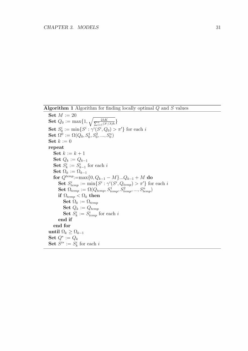
CHAPTER 3. MODELS 31
Algorithm 1 Algorithm for finding locally optimal Q and S values
Set M := 20Set Q0 := max1,
√2λKPn
i=1(λi/λ)h
Set Si
0 := minSi : γi(Si, Q0) > π′ for each iSet Ω0 := Ω(Q0, S
10 , S
20 , ..., S
n0 )
Set k := 0repeat
Set k := k + 1Set Qk := Qk−1
Set Sik := Si
k−1 for each iSet Ωk := Ωk−1
for Qtemp:=max0, Qk−1 −M...Qk−1 + M doSet Si
temp := minSi : γi(Si, Qtemp) > π′ for each iSet Ωtemp := Ω(Qtemp, S
1temp, S
2temp, ..., S
ntemp)
if Ωtemp < Ωk thenSet Ωk := Ωtemp
Set Qk := Qtemp
Set Sik := Si
temp for each iend if
end foruntil Ωk ≥ Ωk−1
Set Q∗ := Qk
Set Si∗ := Sik for each i

CHAPTER 3. MODELS 32
Figure 3.1: Supply Chain Parameters Before and After Contract
Supplier
Installation 1 Installation 2
Lr1 Lr
21
2
hr1 hr
2r1 ,
r’1
r2 ,
r’2
Supplier
Installation 1 Installation 2
Lm1 Lm
21
2
hm1 hm
2r1 ,
r’1
r2 ,
r’2
m
1 , m’1
m2 ,
m’2
Retailer Retailer
A
Before Contract After Contract
Additional notation used in this section is as following:

CHAPTER 3. MODELS 33
λi = Demand arrival rate per time at each installation i,
λ = Combined arrival rate per time,
Lir = Retailer’s replenishment leadtime for installation i,
Lim = Manufacturer’s replenishment leadtime for installation i,
Sir = Base stock level optimizing total cost rate of installation i under the retailer control,
Sim = Base stock level optimizing total cost rate of installation i under the manufacturer control,
rir = Reorder level optimizing total cost rate of installation i under the retailer control,
Qir = Reorder quantity optimizing total cost rate of installation i under the retailer control,
Qm = Reorder quantity optimizing total cost rate system under manufacturer control,
hr = Holding cost per unit per time for the retailer,
hm = Holding cost per unit per time for the manufacturer,
K = Setup cost for ordering,
πr = Backorder cost per occasion observed by the retailer,
π′r = Backorder cost per unit per time observed by the retailer,
πm = Backorder cost per occasion charged by the retailer to the manufacturer,
π′m = Backorder cost per unit per time charged by the retailer to the manufacturer,
Ωr = Total expected cost rate of the retailer before contract
Ωm = Total expected cost rate of the manufacturer before contract
Ωsc = Total expected cost rate of the supply chain before contract
Ωcr = Total expected cost rate of the retailer after contract
Ωcm = Total expected cost rate of the manufacturer after contract
Ωcsc = Total expected cost rate of the supply chain after contract
A = Annual fee paid by the retailer to the manufacturer for the contract.
3.4.1 Without Setup Costs
First we consider the case with no setup costs. Using the base stock model we derive
the total costs of the retailer and the manufacturer. Before the contract, the retailer
manages her own inventory according to her own cost parameters. Supply chain

CHAPTER 3. MODELS 34
cost rate, Ωsc, is equal to the retailer’s cost rate, Ωr. These costs are given below:
Ωr(S) = hrχ(S, Lr) + πrE(S, Lr) + π′rB(S, Lr) (3.34)
Ωm(S) = 0 (3.35)
Ωsc(S) = hrχ(S, Lr) + πrE(S, Lr) + π′rB(S, Lr). (3.36)
Let Sr is the base stock level optimizing retailers total cost rate,
Sr = arg min Ωr(S). (3.37)
After the consignment contract, the manufacturer assumes the control of in-
ventory. In this case, the manufacturer has an improved leadtime, Lm ≤ Lr, and
holding cost per unit per time hm ≤ hr. Using these parameters and the backorder
costs incurred by the retailer, πm and π′m, the manufacturer optimizes Ωcm.
The annual fee payed by retailer to manufacturer is, A. After contract:
Ωcr(S) = (πr − πm)E(S, Lm) + (π′r − π′m)B(S, Lm) + A. (3.38)
Ωcm(S) = hmχ(S, Lm) + πmE(S, Lm) + π′mB(S, Lm)− A. (3.39)
Ωcsc(S) = hmχ(S, Lm) + πrE(S, Lm) + π′rB(S, Lm). (3.40)
Sm is the base stock level optimizing the manufacturer’s after contract total cost
rate,
Sm = arg min Ωcm(S). (3.41)
Supply chain saving that is achieved by the implementation of the contract can
be given as:
= Ωcsc(Sm)− Ωsc(Sr) (3.42)
= (hmχ(Sm, Lm) + πrE(Sm, Lm) + π′rB(Sm, Lm))
− (hr χ(Sr, Lr) + πr E(Sr, Lr) + π′r B(Sr, Lr)).
Note that the supply chain costs are minimized (or the savings are maximized),
i.e., the channel is coordinated, only if the retailer charges the same backorder

CHAPTER 3. MODELS 35
penalties that she observes, i.e., πm = πr and π′m = π′r. Because, only in this case,
the manufacturer (who makes the decision on S) and the supply chain have the
same cost function (i.e., objective function) with the exclusion of the fixed payment
A which does not depend on S.
For the retailer and manufacturer to participate in the contract, both have to be
better off with the contract. Thus, the following conditions should be satisfied.
Ωm(Sr) ≥ Ωcm(Sm). (3.43)
Ωr(Sr) ≥ Ωcr(Sm). (3.44)
These two conditions enforce upper and lower bound constraints on A. If those
two conditions are satisfied, the contract is possible:
A ≥ hmχ(Sm, Lm) + πmE(Sm, Lm) + π′mB(Sm, Lm) (3.45)
A ≤ (hr χ(Sr, Lr) + πr E(Sr, Lr) + π′r B(Sr, Lr)) (3.46)
−(πr − πm)E(Sm, Lm)− (π′r − π′m)B(Sm, Lm).
Note finally that a feasible A can be found, only if the supply chain cost savings
are non-negative. The exact value of A that is used in the contract specifies how the
savings through the contract are allocated to both parties. The backorder penalties
charged by the retailer to the manufacturer also impact the final costs of each party
and thus the allocation of total supply chain costs. However, as discussed before,
backorder penalties that are different from the original backorder penalties result in
a non–coordinated channel, and thus should not be used as an allocation mechanism.
3.4.2 With Setup Costs
Using (r,Q) and (Q,S) models we derive the total costs of retailer and manufacturer
when there are setup costs. Initially each retailer installation use (r,Q) model to
manage their inventories. We assume that there are n installations. Let us define the
following n-vectors for simplicity. First one contains individual ordering quantities
of retailer installations Q= (Q1, Q2, ..., Qn). Second one contains individual reorder

CHAPTER 3. MODELS 36
levels of retailer installations r= (r1, r2, ..., rn). Before the contract the total costs
of eacc party for a given Q and r can be written as:
Ωir(Q
i, ri) = Kλi
Qi+ hrχ(Qi, ri, Li
r) + πrE(Qi, ri, Lir) + π′rB(Qi, ri, Li
r) (3.47)
Ωr(Q, r) =n∑
i=1
Ωir(Q
i, ri) (3.48)
Ωm(Q, r) = 0. (3.49)
Ωsc(Q, r) =n∑
i=1
Ωir(Q
i, ri). (3.50)
For installation i, Let rir and Qi
r denote the reorder quantity and reorder level
that minimizes installation i’s total cost rate, Ωir. Formally,
(Qir, r
ir) = arg min Ωi
r(Qi, ri) for i = 1, ..., n. (3.51)
Then, Qr= (Q1r, Q
2r, ..., Q
nr ) and rr= (r1
r , r2r , ..., r
nr )
The supply chain cost rate, and the total retailer cost rate are equal to the sum
of cost rates of installations, i.e.,
Ωsc(Qr, rr) = Ωr(Qr, rr) =n∑
i=1
Ωir(Q
ir, r
ir). (3.52)
After the consignment contract, the manufacturer assumes the control of inven-
tory. She starts to use (Q,S) policy to jointly replenish installations. In this case
manufacturer has an improved leadtime, Lim ≤ Li
r, setup cost and holding cost,
hm ≤ hr. With these parameters, the backorder costs incurred by retailer, πm and
π′m and for a given (Q,S) , the cost of each party after the contract can be written

CHAPTER 3. MODELS 37
as:
Ωcr(Q,S) =
n∑i=1
(πr − πm)λiP i(Si, Q, Lim) +
n∑i=1
(π′r − π′m)Bi(Si, Q, Lim) + A (3.53)
Ωcm(Q,S) = K
λ
Q+
n∑i=1
(hm)(Si − λi(Q− 1)
2λ− λiLi
m)+ (3.54)
n∑i=1
(π′m + hm)Bi(Si, Q, Lim)+
n∑i=1
πmP i(Si, Q, Lim)− A
Ωcsc(Q,S) = K
λ
Q+
n∑i=1
(hm)(Si − λi(Q− 1)
2λ− λiLi
m)+ (3.55)
n∑i=1
(π′r + hm)Bi(Si, Q, Lim)+
n∑i=1
πrλiP i(Si, Q, Li
m).
Let Qm be the optimal joint ordering quantity and Sim be the optimal base stock
level of each installation. Let Sm= (S1m, S2
m, ..., Snm). Formally,
(Qm,Sm) = arg min Ωcm(Q,S). (3.56)
Supply chain saving that is achieved by the implementation of the contract can be
given as:
Ωsc(Qr, rr)− Ωcsc(Qm,Sm) (3.57)
=n∑
i=1
[K
λi
Qir
+ hrχ(Qir, r
ir, L
ir) + πrE(Qi
r, rir, L
ir) + π′rB(Qi
r, rir, L
ir)
]
−Kλ
Qm
+n∑
i=1
(hm)(Sim −
λi(Qm − 1)
2λ− λiLi
m)+
−n∑
i=1
(π′r + hm)Bi(Sim, Qm, Li
m)+
−n∑
i=1
πrλiP i(Si
m, Qm, Lim).Ωi
r(Qi,

CHAPTER 3. MODELS 38
Note again that the supply chain costs are minimized or the channel is coordinated,
only if the retailer charges the same backorder penalties that she observes, i.e.,
πm = πr and π′m = π′r. Because, only in this case, the manufacturer (who makes
the decision on Q and S) and the supply chain have the same cost function (i.e.,
objective function).
For the retailer and the manufacturer to participate in the contract, both have
to be better off with the contract. Thus, the following conditions should be satisfied.
Ωr(Qr, rr) ≥ Ωcr(Qm,Sm) (3.58)
Ωm(Qr, rr) ≥ Ωcm(Qm,Sm). (3.59)
These two conditions enforce upper and lower bound constraints on A. These
bounds are:
A ≥Kλ
Qm
+n∑
i=1
(hm)(Sim −
λi(Qm − 1)
2λ− λiLi
m) (3.60)
+n∑
i=1
(π′m + hm)Bi(Sim, Qm, Li
m)
+n∑
i=1
πmλiP i(Sim, Qm, Li
m)
A ≤n∑
i=1
[K
λi
Qir
+ hrχ(Qir, r
ir, L
ir) + πrE(Qi
r, rir, L
ir) + π′rB(Qi
r, rir, L
ir)
](3.61)
−n∑
i=1
(πr − πm)λiP i(Sim, Qm, Li
m)−n∑
i=1
(π′r − π′m)Bi(Sim, Qm, Li
m).
Note once again that a feasible A can be found, only if the supply chain cost
savings are non-negative. The exact value of A specifies how the savings through
the contract are allocated to the parties in the supply chain.

Chapter 4
Contracts Without Setup Costs
In this chapter, we construct and examine various contracts using the base stock
model we introduced in Section ??. We build four base cases to differentiate situa-
tions where different types of backorders (Type I or Type II) and different backorder
costs (high or low) are incurred. In Table 4.1, base case parameters and in Table 4.2,
the optimal solutions of base cases are given. Exact cost expressions are calculated
using a program coded in C++ and Matlab and optimal solutions are found through
enumeration. We take λ = 5 and A = 0 for all cases that we examine.
Table 4.1: Physical Improvement Base Case Parameters
Base Case Lr hr πr π′r K
1 2 6 100 0 0
2 2 6 0 100 0
3 2 6 50 0 0
4 2 6 0 50 0
39

CHAPTER 4. CONTRACTS WITHOUT SETUP COSTS 40
Table 4.2: Physical Improvement Base Case Optimal Sr and Cost Components
Cost Components
Base Case Sr Ordering Holding BO1 BO2 Total
1 14 0 25.122 8.346 0 33.468
2 15 0 30.621 0 10.348 40.969
3 12 0 15.186 10.422 0 25.608
4 14 0 25.122 0 9.347 34.469
In Section 4.1, we analyze savings achieved through physical improvement. As
we mentioned before, physical improvement consists of holding cost reduction and
leadtime improvement. We analyze the savings achieved through leadtime reduction
in Section 4.1.1, and through holding cost reduction, in Section 4.1.2. In Section 4.2,
we examine the impact of the retailer charging different backorder costs on supply
chain costs when physical improvements are provided. Physical improvements are
obtained through leadtime reduction in Section 4.2.1, and through leadtime reduc-
tion in Section 4.2.2.
4.1 Physical Improvement Under Centralized
Control
In this section we analyze physical improvements achieved through centralized con-
trol. Base cases exhibit before contract situations. After the manufacturer assumes
control, the system is improved through either leadtime reduction or holding cost
reduction. More savings would be achieved, if leadtime and holding cost were re-
duced at the same time, but in that case the marginal effects of those would not
be captured. So each table is constructed by varying a single parameter. The cost
structure of a single the retailer under base stock policy and cost expressions of par-
ties after contract is given in Chapter 3. For the sake of simplicity, in this section
we consider there is a single the retailer installation and its control is assumed by
the manufacturer after the contract. Under centralized control, the backorder cost

CHAPTER 4. CONTRACTS WITHOUT SETUP COSTS 41
parameters that the manufacturer observes are exactly equal to the backorder cost
parameters that the retailer sees. In other words, the retailer truly reflects its own
backorder costs under centralized control and the retailer and the manufacturer act
as a single entity. The channel costs are simply equal to the manufacturer’s cost.
4.1.1 Leadtime Reduction
Table 4.3: Base Case 1 Percentage Savings - Leadtime Reduction
Base Case 1 Cost Components
Lm Sm Ordering Holding BO1 BO2 Total % Savings Abs. Diff.
0.5 5 0 15.372 4.202 0 19.574 41.515 13.894
0.75 6 0 14.379 8.628 0 23.007 31.256 10.461
1 8 0 18.733 6.809 0 25.542 23.683 7.926
1.25 9 0 17.717 10.221 0 27.938 16.524 5.530
1.5 11 0 21.969 7.924 0 29.893 10.680 3.574
1.75 12 0 20.916 10.680 0 31.596 5.594 1.872
2 14 0 25.122 8.346 0 33.468 0 0
In Table 4.3, we consider base case 1. In this base case a high per occasion backo-
rder cost (Type I) is incurred. At each step Lm is reduced 0.25 units. It is observed
that, as leadtime gets smaller, the base stock level and the total cost decreases.
However note that not all cost components decrease as the leadtime gets smaller.
As Lm is decreased from 2 to 1.25, BO1 increases from 8.346 to 10.221. But this
increase is compensated by a larger decrease in holding cost where holding cost de-
crease from 25.122 to 17.717, so positive savings are achieved. A similar behavior
can be observed in holding costs. As Lm is decreased from 1.25 to 1, holding cost
increases from 17.717 to 18.733. This is due to discontinuous structure of the cost
function. At discontinuity points, sudden shifts in backorder cost terms and holding
cost terms are observed. This type of behavior is also in other cases later in this
chapter. At most 41.515% savings are achieved when Lm is decreased to 0.5. The
improvements achieved by reducing leadtime can also be observed through examin-
ing absolute differences in costs and those differences are given in Table 4.3. The

CHAPTER 4. CONTRACTS WITHOUT SETUP COSTS 42
absolute differences show a similar pattern to percentage savings.
Before going further, using the data we presented for base case 1, we calculate
the bounds for the annual fee, A. Total cost presented in Table 4.3, provides a lower
bound for the annual payment since for any fee less than relevant total cost, man-
ufacturer has a positive cost, which is greater than her initial cost, 0. This implies
that, any payment less than the lower bound is not profitable for the manufacturer.
Similarly, for any fee that is greater than the initial cost of the retailer, 33.468, the
partnership is not profitable for the retailer. For participation of both, the annual
payment shall be between, the manufacturer cost and the initial retailer cost. The
bounds for this base case is presented in Table 4.4.
Table 4.4: Base Case 1 Annual Payment Bounds - Leadtime Reduction
Lm Lower B. Upper B.
0.5 19.574 33.468
0.75 23.007 33.468
1 25.542 33.468
1.25 27.938 33.468
1.5 29.893 33.468
1.75 31.596 33.468
2 33.468 33.468
As it can be seen in Table 4.4, as leadtime is improved, the lower bound for
the range decreases which creates a larger range for annual payment which in turn
creates an increased opportunity for a contract. This result can be repeated for
all numerical data that we present. We should note here that the annual payment
alone may not be enough to determine whether the retailer or the manufacturer
will participate in the contract. As we mentioned before, both retailer and the
manufacturer may have additional benefits such as the strengthened market share
for the manufacturer and the ability to divert the focus to its own operations for the
retailer. Thus, the manufacturer or the retailer may still want to participate even
though they may be increasing their operational costs.
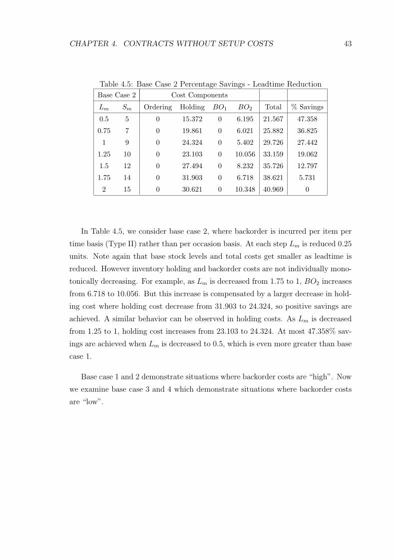
CHAPTER 4. CONTRACTS WITHOUT SETUP COSTS 43
Table 4.5: Base Case 2 Percentage Savings - Leadtime Reduction
Base Case 2 Cost Components
Lm Sm Ordering Holding BO1 BO2 Total % Savings
0.5 5 0 15.372 0 6.195 21.567 47.358
0.75 7 0 19.861 0 6.021 25.882 36.825
1 9 0 24.324 0 5.402 29.726 27.442
1.25 10 0 23.103 0 10.056 33.159 19.062
1.5 12 0 27.494 0 8.232 35.726 12.797
1.75 14 0 31.903 0 6.718 38.621 5.731
2 15 0 30.621 0 10.348 40.969 0
In Table 4.5, we consider base case 2, where backorder is incurred per item per
time basis (Type II) rather than per occasion basis. At each step Lm is reduced 0.25
units. Note again that base stock levels and total costs get smaller as leadtime is
reduced. However inventory holding and backorder costs are not individually mono-
tonically decreasing. For example, as Lm is decreased from 1.75 to 1, BO2 increases
from 6.718 to 10.056. But this increase is compensated by a larger decrease in hold-
ing cost where holding cost decrease from 31.903 to 24.324, so positive savings are
achieved. A similar behavior can be observed in holding costs. As Lm is decreased
from 1.25 to 1, holding cost increases from 23.103 to 24.324. At most 47.358% sav-
ings are achieved when Lm is decreased to 0.5, which is even more greater than base
case 1.
Base case 1 and 2 demonstrate situations where backorder costs are “high”. Now
we examine base case 3 and 4 which demonstrate situations where backorder costs
are “low”.

CHAPTER 4. CONTRACTS WITHOUT SETUP COSTS 44
Table 4.6: Base Case 3 Percentage Savings - Leadtime Reduction
Base Case 3 Cost Components
Lm Sm Ordering Holding BO1 BO2 Total % Savings
0.5 4 0 10.025 5.441 0 15.466 39.605
0.75 5 0 9.442 8.856 0 18.298 28.546
1 7 0 13.533 6.669 0 20.201 21.112
1.25 8 0 12.794 8.981 0 21.775 14.965
1.5 9 0 12.138 11.180 0 23.317 8.945
1.75 11 0 15.956 8.672 0 24.628 3.826
2 12 0 15.186 10.422 0 25.608 0
In Table 4.6, we consider base case 3, where backorder cost incurred per occasion
basis as in base case 1. At each step Lm is reduced 0.25 units. Results are similar
to those in base case 1 are observed. The percentage savings in this case are less
than the percentage savings in base case 1 for some lead time values and more than
the percentage savings in base case 1 for some other lead time values.
Table 4.7: Base Case 4 Percentage Savings, Leadtime Reduction
Base Case 4 Cost Components
Lm Sm Ordering Holding BO1 BO2 Total % Savings
0.5 5 0 15.372 0 3.098 18.469 46.417
0.75 6 0 14.379 0 7.325 21.703 37.034
1 8 0 18.733 0 6.106 24.838 27.940
1.25 9 0 17.717 0 10.138 27.855 19.189
1.5 11 0 21.969 0 8.078 30.047 12.827
1.75 12 0 20.916 0 11.797 32.712 5.096
2 14 0 25.122 0 9.347 34.469 0
In Table 4.7, we consider base case 4, where backorder is incurred per unit per
time basis as base case 2. At each step Lm is reduced 0.25 units. The results are
similar to those in base case 2.

CHAPTER 4. CONTRACTS WITHOUT SETUP COSTS 45
Note that leadtime reduction brings more percentage savings in cases where Type
II backorder is incurred (base case 2 and 4) than cases where Type I backorder is
incurred (base case 1 and 3). This is due to the fact that charging a fixed penalty
per unit per time is more prohibitive than charging the same penalty per occasion.
Hence lead time reduction is more effective and savings are more for the case of Type
II backorder costs. We see that the difference between percentage savings decline
(in percentage) as the leadtime reductions gets larger.
4.1.2 Holding Cost Reduction
Table 4.8: Base Case 1 Percentage Savings - Holding Cost Reduction
Base Case 1 Cost Components
hm Sm Ordering Holding BO1 BO2 Total % Savings
3 15 0 15.310 4.874 0 20.184 39.690
3.25 15 0 16.586 4.874 0 21.460 35.877
3.5 15 0 17.862 4.874 0 22.736 32.065
3.75 15 0 19.138 4.874 0 24.012 28.253
4 14 0 16.748 8.346 0 25.094 25.021
4.25 14 0 17.794 8.346 0 26.140 21.893
4.5 14 0 18.841 8.346 0 27.187 18.766
4.75 14 0 19.888 8.346 0 28.234 15.638
5 14 0 20.935 8.346 0 29.281 12.510
5.25 14 0 21.981 8.346 0 30.327 9.383
5.5 14 0 23.028 8.346 0 31.374 6.255
5.75 14 0 24.075 8.346 0 32.421 3.128
6 14 0 25.122 8.346 0 33.468 0
In Table 4.8, we consider base case 1. In this base case a high per occasion backorder
cost (Type I) is incurred. At each step hm is reduced 0.25 units. It is observed that
optimal base stock level chosen by the manufacturer, Sm increases since holding
inventory becomes less costly. Sm increases from 14 to 15, meanwhile holding cost
decreases from 25.122 to 15.310 as hm is reduced to 3 from 6. As expected total cost

CHAPTER 4. CONTRACTS WITHOUT SETUP COSTS 46
decreases in this direction. The same tradeoff between holding costs and backorder
costs is observed here as it is observed in leadtime reduction cases. As hm is reduced
to 3.75 from 4, inventory cost increases to 19.138 from 16.748 meanwhile BO1 de-
creases to 4.874 from 8.346, which compensates the increase in holding costs and
positive savings are achieved. Unlike leadtime reduction case the backorder costs
decrease in monotonic manner as holding cost decreases. At most 39.690% savings
are achieved when hm is decreased to 3.
Similar to what we did in Section 4.1.1, we calculate the bounds for the annual
fee, A, for base case 1. Total cost presented in Table 4.9, provides a lower bound
for the annual payment since for any fee less than relevant total cost, manufacturer
has a positive cost, which is greater than her initial cost, 0. This implies that, any
payment less than the lower bound is not profitable for the manufacturer. Similarly,
for any fee that is greater than the initial cost of the retailer, 33.468, the partnership
is not profitable for the retailer. For participation of both, the annual payment shall
be between, the manufacturer cost and the initial retailer cost. The bounds for this
base case is presented in Table 4.9.
Table 4.9: Base Case 1 Annual Payment Bounds - Holding Cost Reduction
hm Lower B. Upper B.
3 20.184 33.468
3.25 21.460 33.468
3.5 22.736 33.468
3.75 24.012 33.468
4 25.094 33.468
4.25 26.140 33.468
4.5 27.187 33.468
4.75 28.234 33.468
5 29.281 33.468
5.25 30.327 33.468
5.5 31.374 33.468
5.75 32.421 33.468
6 33.468 33.468

CHAPTER 4. CONTRACTS WITHOUT SETUP COSTS 47
As it can be seen in Table 4.9, as holding cost is improved, the lower bound for
the range decreases which creates a larger range for annual payment which in turn
creates an increased opportunity for a contract.
Table 4.10: Base Case 2 Percentage Savings - Holding Cost Reduction
Base Case 2 Cost Components
hm Sm Ordering Holding BO1 BO2 Total % Savings
3 16 0 18.164 0 5.474 23.638 42.302
3.25 16 0 19.678 0 5.474 25.152 38.607
3.5 16 0 21.192 0 5.474 26.666 34.913
3.75 16 0 22.705 0 5.474 28.179 31.218
4 16 0 24.219 0 5.474 29.693 27.523
4.25 16 0 25.733 0 5.474 31.207 23.828
4.5 16 0 27.246 0 5.474 32.720 20.134
4.75 16 0 28.760 0 5.474 34.234 16.439
5 16 0 30.274 0 5.474 35.748 12.744
5.25 15 0 26.793 0 10.348 37.141 9.343
5.5 15 0 28.069 0 10.348 38.417 6.228
5.75 15 0 29.345 0 10.348 39.693 3.114
6 15 0 30.621 0 10.348 40.969 0
In Table 4.10, we consider base case 2. At each step hm is reduced 0.25 units.
In this base case a high per unit per time backorder cost (Type II) is incurred. As
holding cost is reduced, Sm increases since now more inventory could be kept with
less lower cost. Consequently backorder costs decline. As base stock level shifts from
15 to 16, holding cost increases slightly but this is compensated by a sharp decrease
in backorder cost likewise in base case 1. At most 42.302% savings are achieved
when hm is decreased to 3. Note that more percentage savings is achieved than base
case 1 due to difference in types of backorders. Similar to our findings in Section
4.1.1, this time reduction in holding cost brings more savings when backorders are
incurred on per unit per time basis.

CHAPTER 4. CONTRACTS WITHOUT SETUP COSTS 48
Table 4.11: Base Case 3 Percentage Savings - Holding Cost Reduction
Base Case 3 Cost Components
hm Sm Ordering Holding BO1 BO2 Total % Savings
3 14 0 12.561 4.173 0 16.734 34.653
3.25 13 0 10.798 6.777 0 17.575 31.368
3.5 13 0 11.629 6.777 0 18.406 28.124
3.75 13 0 12.459 6.777 0 19.236 24.880
4 13 0 13.290 6.777 0 20.067 21.637
4.25 13 0 14.120 6.777 0 20.897 18.393
4.5 13 0 14.951 6.777 0 21.728 15.149
4.75 12 0 12.022 10.422 0 22.444 12.354
5 12 0 12.655 10.422 0 23.077 9.884
5.25 12 0 13.287 10.422 0 23.709 7.413
5.5 12 0 13.920 10.422 0 24.342 4.942
5.75 12 0 14.553 10.422 0 24.975 2.471
6 12 0 15.186 10.422 0 25.608 0
In Table 4.11, we consider base case 3. In this base case a low per occasion
backorder cost (Type I) is incurred. As holding cost is reduced, Sm increases since
now more inventory could be kept with less price. Consequently backorder costs
reduce since now there are less stockout situations. As base stock level shifts values
(such as 12 to 13, 13 to 14), holding cost increases slightly but this is compensated
by a sharp decrease in backorder cost as observed in base case 1 and 2. At most
34.653% savings are achieved when hm is decreased to 3.

CHAPTER 4. CONTRACTS WITHOUT SETUP COSTS 49
Table 4.12: Base Case 4 Percentage Savings, Holding Cost Reduction
Base Case 4 Cost Components
hm Sm Ordering Holding BO1 BO2 Total % Savings
3 15 0 15.310 0 5.174 20.484 40.571
3.25 15 0 16.586 0 5.174 21.760 36.869
3.5 15 0 17.862 0 5.174 23.036 33.168
3.75 15 0 19.138 0 5.174 24.312 29.466
4 15 0 20.414 0 5.174 25.588 25.765
4.25 15 0 21.690 0 5.174 26.864 22.063
4.5 15 0 22.966 0 5.174 28.140 18.362
4.75 14 0 19.888 0 9.347 29.235 15.184
5 14 0 20.935 0 9.347 30.282 12.147
5.25 14 0 21.981 0 9.347 31.328 9.110
5.5 14 0 23.028 0 9.347 32.375 6.074
5.75 14 0 24.075 0 9.347 33.422 3.037
6 14 0 25.122 0 9.347 34.469 0
In Table 4.12, we consider base case 4. In this base case a low per unit per time
backorder cost (Type II) is incurred. At each step hm is reduced 0.25 units. The
results are similar to those in Table 4.10 for base case 2. At most 40.571% savings
are achieved when hm is decreased to 3. Again from comparison of base case 3 and
4 under holding cost reduction, it can be deduced that holding cost improvement
brings more percentage savings when Type II backorder costs are incurred.
Until now, we have shown that considerable savings are achievable through phys-
ical improvement. Both leadtime reduction and holding cost reduction can be used
to achieve savings around 40% when Lm is reduced to 0.5 from 4 or hm is reduced to
3 from 6. Another result that we identified is when backorders are “high”, physical
improvement brings more percentage savings. We have also shown that physical
improvement works better when backorder costs are incurred on per unit per time
basis rather than per occasion basis. We identified that the discontinuity shifts in
Sm, causes sudden increases in holding costs and decreases backorder costs. In our
data sets, holding cost reduction brought more savings than leadtime improvement.

CHAPTER 4. CONTRACTS WITHOUT SETUP COSTS 50
As holding cost is reduced, inventory levels increase while cost of holding such large
inventories decrease which in turn reduces the backorders due to decreased number
of stockouts. But in leadtime reduction case, as base stock levels decrease due to
shorter leadtime, the backorders may increase and hamper the savings. In the next
section we investigate the situation where the retailer manipulates backorder costs
to achieve savings and the “limits” to this manipulation.
4.2 Decentralized Control
In this section, we study the impact of the retailer charging a different backorder
penalty than what she observes on coordination of the channel. As we defined in
Chapter 3, the retailer pays her customers πr and π′r but in the contract she may
charge the manufacturer backorder costs which are different (i.e. πm 6= πr and π′m 6=π′r). This manipulation can be done in various ways. First the backorder cost may be
changed without changing the type of the backorder cost. For example, if the retailer
is charged per occasion basis by customer, the retailer may charge the manufacturer
again on per occasion basis but with a different cost. Second, the retailer may charge
a different type of backorder cost (possibly with a different amount than what she
faces) to the manufacturer, such as charging Type II backorder cost while observing
Type I backorder cost. Again we define 4 base cases to demonstrate behavior of
cost functions of the retailer, the manufacturer and supply chain. The backorder
cost ranges that are incurred to the manufacturer are given in the Table 4.13. The
optimal solution of base cases before contract are given in Table 4.14.
Table 4.13: Decentralized Channel - Base Case ParametersBase Case Lr hr πr π′r K πm π′m K
1 2 6 0 100 0 0 [50, 150] 0
2 2 6 0 50 0 0 [25, 75] 0
3 2 6 50 0 0 [25, 75] 0 0
4 2 6 0 50 0 [50, 150] 0 0

CHAPTER 4. CONTRACTS WITHOUT SETUP COSTS 51
Table 4.14: Decentralized Channel - Base Case Optimal Sr and Cost Components
Cost Components
Base Case Sr Ordering Holding BO1 BO2 Total
1 15 0 30.621 0 10.348 40.969
2 14 0 25.122 0 9.347 34.469
3 12 0 15.186 10.422 0 25.608
4 14 0 25.122 0 9.347 34.469
In Section 4.2.1, we investigate the situation when the physical improvement is
achieved through leadtime reduction. In Section 4.2.2, we repeat the same analysis
in a setting where physical improvement is achieved through holding cost reduction.
4.2.1 Decentralized Control with Leadtime Reduction
Table 4.15: Base Case 1 Percentage Savings, Lm = 1.5, π′m changes
Total Costs Savings
π′m Retailer Manufacturer Supply Chain %
50 8.078 30.047 38.125 6.9
60 6.462 31.663 38.125 6.9
70 2.470 33.256 35.726 12.8
80 1.646 34.080 35.726 12.8
90 0.823 34.903 35.726 12.8
100 0 35.726 35.726 12.8
110 -0.823 36.549 35.726 12.8
120 -1.646 37.372 35.726 12.8
130 -2.470 38.196 35.726 12.8
140 -1.586 38.789 37.203 9.2
150 -1.983 39.185 37.203 9.2
In Table 4.15, we consider base case 1. When the manufacturer assumes the control,
leadtime is reduced to 1.5. Type II backorder cost charged by the retailer to the

CHAPTER 4. CONTRACTS WITHOUT SETUP COSTS 52
manufacturer, is iterated between 50 and 150 with increments of 10. The costs of
the manufacturer, the retailer and channel are also given in the table 4.15. Note that
these costs exclude the annual fee that is paid by the retailer to the manufacturer.
Even if the retailer charges the manufacturer π′m = 50, which is much less than
what she observes, positive channel savings are possible (6.9%). This indicates the
considerable effect of leadtime reduction. When 70 ≤ π′m ≤ 130, minimum channel
cost, 35.726, and maximum percentage savings in the channel, 12.8%, are achieved.
For π′m > 100, the retailer “earns” money from backorders, which explains the
negative values that is seen in the retailer’s costs. Note that for those values, the
manufacturer’s cost is greater than the channel cost. As for backorder costs that are
greater 130 and smaller than 70, channel savings diminish to 9.2 and 6.9 respectively
from 12.8. An important observation is that channel coordination is achieved in an
interval around π′m = 100. We obtained an interval for πm where all values in that
interval, coordinate the channel. Note that the channel is coordinated for a range
of πm values and π′m = 100, which is also equal to π′r, is in that interval too.
Table 4.16: Base Case 2 Percentage Savings, Lm = 1.5, π′m changes
Total Costs Savings
π′m Retailer Manufacturer Supply Chain %
25 7.483 24.279 31.762 7.9
30 5.986 25.776 31.762 7.9
35 4.490 27.272 31.762 7.9
40 1.616 28.432 30.047 12.8
45 0.808 29.240 30.047 12.8
50 0 30.047 30.047 12.8
55 -0.808 30.855 30.047 12.8
60 -1.616 31.663 30.047 12.8
65 -2.423 32.471 30.047 12.8
70 -1.646 33.256 31.610 8.3
75 -2.058 33.668 31.610 8.3
In Table 4.16, we consider base case 2. This case is very similar to base case
1, only difference is this time the retailer faces a lower Type II backorder cost.

CHAPTER 4. CONTRACTS WITHOUT SETUP COSTS 53
Again leadtime is reduced to 1.5 under the manufacturer control. Type II backorder
cost charged by the retailer to the manufacturer, is iterated between 25 and 75
by increments of 5. The costs of the manufacturer, the retailer and channel are
given in the table 4.16. As it is shown in the table, even if the retailer charges the
manufacturer π′m = 25, which is much less than what she observes, positive channel
savings are possible (7.9%). When 40 ≤ π′m ≤ 65, minimum channel cost, 30.047,
and maximum percentage savings in the channel, 12.8%, are achieved. For π′m > 65,
the retailer “earns” money from backorders, which explains the negative values that
is seen in the retailer’s costs. Note that for those values, the manufacturer’s cost
is greater than the channel cost. As for backorder costs that are greater than 65
and smaller than 40, channel savings diminish to 8.3 and 7.9 respectively from
12.8. Again channel coordination is achieved in an interval around π′m = 50 which
supports our observation in base case 1. Note that similar percentage savings are
achieved as base case 1.
Table 4.17: Base Case 3 Percentage Savings, Lm = 1.5, πm changes
Total Costs Savings
πm Retailer Manufacturer Supply Chain %
25 8.451 16.616 25.067 2.1
30 6.761 18.307 25.067 2.1
35 3.354 19.963 23.317 8.9
40 2.236 21.081 23.317 8.9
45 1.118 22.199 23.317 8.9
50 0 23.317 23.317 8.9
55 -0.689 24.373 23.684 7.5
60 -1.378 25.062 23.684 7.5
65 -2.066 25.75 23.684 7.5
70 -2.755 26.439 23.684 7.5
75 -3.444 27.128 23.684 7.5
In Table 4.17, we consider base case 3. In this case the retailer faces a lower Type
I backorder cost. Leadtime is reduced to 1.5 under the manufacturer control. Type
I backorder cost charged by the retailer to the manufacturer, is iterated between

CHAPTER 4. CONTRACTS WITHOUT SETUP COSTS 54
25 and 75 by increments of 5. The costs of the manufacturer, the retailer and
channel are given in the Table 4.17. The results are similar to those for base case
1. The maximum savings are possible when the retailer charges the same backorder
penalties that she observes.
Table 4.18: Base Case 4 Percentage Savings, Lm = 1.5, πm changes
Total Costs Savings
πm Retailer Manufacturer Supply Chain %
25 34.597 16.616 51.213 -48.6
30 32.907 18.307 51.213 -48.6
35 18.320 19.963 38.284 -11.1
40 17.202 21.081 38.284 -11.1
45 16.084 22.199 38.284 -11.1
50 14.967 23.317 38.284 -11.1
55 7.389 24.373 31.762 7.9
60 6.700 25.062 31.762 7.9
65 6.012 25.75 31.762 7.9
70 5.323 26.439 31.762 7.9
75 4.634 27.128 31.762 7.9
80 3.945 27.817 31.762 7.9
85 3.256 28.506 31.762 7.9
90 0.946 29.101 30.047 12.8
95 0.550 29.497 30.047 12.8
100 0.154 29.893 30.047 12.8
105 -0.242 30.290 30.047 12.8
110 -0.638 30.686 30.047 12.8
115 -1.035 31.082 30.047 12.8
120 -1.431 31.478 30.047 12.8
125 -1.827 31.874 30.047 12.8
130 -2.223 32.271 30.047 12.8
135 -2.619 32.667 30.047 12.8
140 -3.016 33.063 30.047 12.8
145 -3.412 33.459 30.047 12.8
150 -3.808 33.855 30.047 12.8

CHAPTER 4. CONTRACTS WITHOUT SETUP COSTS 55
In Table 4.18, we consider base case 4. In this base case, the retailer faces
Type II backorder and incurs Type I backorder to the manufacturer. This scenario
demonstrates a case where the retailer maybe facing backorder costs on a per unit
per time basis, but measurement of this fact is not possible or practical under a
contract. Therefore, the manufacturer is only charged by each occurrence of a
backorder. Leadtime is reduced to 1.5 under the manufacturer control. Type I
backorder cost charged by the retailer to the manufacturer, is iterated between 25
and 150 by increments of 5. The costs of the manufacturer, the retailer and channel
are given in the Table 4.18. Unlike the previous base cases, if the retailer charges
too low, the channel may be worse off. For example if πm = 25, channel costs
increase by 48.6%. This happens even though 50% reduction in leadtime is obtained
under manufacturer control. When a stockout is realized, the retailer pays a greater
cost every item that is included in that backorder and this fact is unobserved to
the manufacturer. For this reason the retailer must find an appropriate backorder
penalty to charge the manufacturer and force her to keep more stock. The results
given in Table 4.18 shows that the maximum channel savings, 12.8% and minimum
channel cost, 30.047, are achieved when 90 ≤ πm ≤ 150.

CHAPTER 4. CONTRACTS WITHOUT SETUP COSTS 56
4.2.2 Decentralized Control with Holding Cost Reduction
Table 4.19: Base Case 1 Percentage Savings, hm = 4, π′m changes
Total Costs Savings
π′m Retailer Manufacturer Supply Chain %
50 5.174 25.588 30.762 24.9
60 4.139 26.623 30.762 24.9
70 3.104 27.658 30.762 24.9
80 1.095 28.598 29.693 27.5
90 0.547 29.146 29.693 27.5
100 0 29.693 29.693 27.5
110 -0.547 30.240 29.693 27.5
120 -1.095 30.788 29.693 27.5
130 -1.642 31.335 29.693 27.5
140 -2.190 31.883 29.693 27.5
150 -1.385 32.266 30.881 24.6
In Table 4.19, we consider base case 1. When the manufacturer assumes the control,
holding cost is reduced to 4. Type II backorder cost charged by the retailer to the
manufacturer, is iterated between 50 and 150 by increments of 10. The costs of
the manufacturer, the retailer and channel are also given in the table 4.19. As it
is shown in the table, even if the retailer charges the manufacturer π′m = 50, which
is much less than what she observes, positive channel savings are possible (24.9%).
This indicates the even more greater than the effect of holding cost reduction. When
80 ≤ π′m ≤ 140, minimum channel cost, 29.693, and maximum percentage savings
in the channel, 27.5%, are achieved. For π′m > 100, the retailer “earns” money from
backorders, which explains the negative values that is seen in the retailer’s costs.
Note that for those values, the manufacturer’s cost is greater than the channel cost.
An important observation is that channel coordination is achieved in an interval
around π′m = 100. We obtained an interval for πm where all values in that interval,
coordinate the channel. As for backorder costs that are greater 140 and smaller than
80, channel savings diminish to 24.6% and 24.9% respectively from 27.5%.

CHAPTER 4. CONTRACTS WITHOUT SETUP COSTS 57
Table 4.20: Base Case 2 Percentage Savings, hm = 4, π′m changes
Total Costs Savings
π′m Retailer Manufacturer Supply Chain %
25 8.062 21.352 29.413 14.7
30 3.739 22.356 26.095 24.3
35 2.804 23.291 26.095 24.3
40 1.869 24.225 26.095 24.3
45 0.517 25.071 25.588 25.8
50 0 25.588 25.588 25.8
55 -0.517 26.105 25.588 25.8
60 -1.035 26.623 25.588 25.8
65 -1.552 27.140 25.588 25.8
70 -2.070 27.658 25.588 25.8
75 -2.587 28.175 25.588 25.8
In Table 4.20, we consider base case 2. This case is very similar to base case 1,
only difference is this time the retailer faces a lower Type II backorder cost. Again
holding cost is reduced to 4 under the manufacturer control. Type II backorder
cost charged by the retailer to the manufacturer, is iterated between 25 and 75 by
increments of 5. The results are similar to those obtained in Table 4.19, except this
time, the channel is coordinated in a wider range.

CHAPTER 4. CONTRACTS WITHOUT SETUP COSTS 58
Table 4.21: Base Case 3 Percentage Savings, hm = 4, πm changes
Total Costs Savings
πm Retailer Manufacturer Supply Chain %
25 7.581 14.917 22.498 12.1
30 4.169 16.377 20.546 19.8
35 3.127 17.419 20.546 19.8
40 2.084 18.461 20.546 19.8
45 0.678 19.389 20.067 21.6
50 0 20.067 20.067 21.6
55 -0.678 20.745 20.067 21.6
60 -1.355 21.422 20.067 21.6
65 -2.033 22.100 20.067 21.6
70 -1.669 22.590 20.921 18.3
75 -2.087 23.007 20.921 18.3
In Table 4.21, we consider base case 3. In this case the retailer faces a lower Type
I backorder cost. Holding cost is reduced to 4 under the manufacturer control. Type
I backorder cost charged by the retailer to the manufacturer, is iterated between 25
and 75 by increments of 5. The costs of the manufacturer, the retailer and channel
are given in the Table 4.21. As it is shown in the table, even if the retailer charges
the manufacturer πm = 25, which is much less than what she observes, positive
channel savings are possible (12.1%). This again indicates the effect of leadtime
reduction. When 45 ≤ πm ≤ 65, minimum channel cost, 20.067, and maximum
percentage savings in the channel, 21.6%, are achieved. For πm > 50, the retailer
“earns” money from each stockout situation, which explains the negative values
that is seen in the retailer’s costs. In this case lower overall savings are achieved
due to change in the backorder cost type. Channel coordination is achieved in an
interval around the original per occasion backorder cost, πr = 50, which supports
that without the retailer manipulating backorder costs, the channel has the most
savings.

CHAPTER 4. CONTRACTS WITHOUT SETUP COSTS 59
Table 4.22: Base Case 4 Percentage Savings, hm = 4, πm changes
Total Costs Savings
πm Retailer Manufacturer Supply Chain %
25 34.127 14.917 49.044 -42.3
30 20.293 16.377 36.670 -6.4
35 19.251 17.419 36.670 -6.4
40 18.208 18.461 36.670 -6.4
45 10.024 19.389 29.413 14.7
50 9.347 20.067 29.413 14.7
55 8.669 20.745 29.413 14.7
60 7.991 21.422 29.413 14.7
65 7.313 22.100 29.413 14.7
70 3.505 22.590 26.095 24.3
75 3.088 23.007 26.095 24.3
80 2.670 23.425 26.095 24.3
85 2.253 23.842 26.095 24.3
90 1.836 24.259 26.095 24.3
95 1.418 24.676 26.095 24.3
100 1.001 25.094 26.095 24.3
105 0.584 25.511 26.095 24.3
110 -0.187 25.775 25.588 25.8
115 -0.431 26.019 25.588 25.8
120 -0.675 26.263 25.588 25.8
125 -0.919 26.506 25.588 25.8
130 -1.162 26.75 25.588 25.8
135 -1.406 26.994 25.588 25.8
140 -1.650 27.238 25.588 25.8
145 -1.893 27.481 25.588 25.8
150 -2.137 27.725 25.588 25.8
In Table 4.22, we consider base case 4. In this base case, the retailer faces Type
II backorder cost and incurs Type I backorder cost to the manufacturer. Holding
cost is reduced to 4 under the manufacturer control. Type I backorder cost charged

CHAPTER 4. CONTRACTS WITHOUT SETUP COSTS 60
by the retailer to the manufacturer, is iterated between 25 and 150 by increments
of 5. The costs of the manufacturer, the retailer and channel are given in the Table
4.22. Unlike the previous base cases, if the retailer charges too low, the channel
loses money, even though the cost of owning the inventory is reduced considerably
under manufacturer’s control. For example if πm = 25, channel savings increase by
is 42.3%. In order to obtain savings for the channel, the retailer needs to find an
appropriate Type I backorder penalty. The results given in Table 4.22 supports this
identification since maximum channel savings, 25.8% and minimum channel cost,
25.588, is achieved when 110 ≤ πm ≤ 150.

Chapter 5
Contracts with Setup Costs
In this chapter, we conduct a numerical study for the case when there are positive
setup costs for ordering. Before the contract, the retailer manages multiple instal-
lations independently using (r,Q) policy at each installation. After the contract,
the manufacturer takes over the control, and manages multiple installations jointly
using a (Q,S) policy. The mathematical analysis of (r,Q) and (Q,S) policies are
given in Chapter 3. In Section 5.1, we study the impact of the joint replenishment
alone on supply chain costs when the supply chain is under centralized control. In
Section 5.2, in addition to the ability to jointly replenish multiple installations, the
impact of further improvement through lead time reduction and inventory holding
cost reduction is studied. In Section 5.3, we consider a decentralized control scenario
and study the impact of the retailer charging backorder penalties different than she
observers.
For simplicity, we assume that the retailer has two identical installations. Hence,
the optimal policy parameters are also identical for these installations. The retailer
or supply chain costs before the contract in all numerical examples in this chapter
refer to the total cost in both installations (two times total cost of a single instal-
lation). Note that base stock level, Sm, stands for base stock levels at a single
installation. In all numerical examples, we assume A = 0.
61

CHAPTER 5. CONTRACTS WITH SETUP COSTS 62
5.1 Effect of Pure JRP
In this section we assume the centralized control of the chain, thus the backorder
penalties that are exactly equal to backorder penalties that the retailer observes.
Also there are no physical improvements in the system. Hence, πm = πr, π′m = π′r,
hm = hr and Lm = Lr. We quantify the savings of the channel when manufacturer
jointly manages inventories and uses (Q,S) policy instead of (r,Q) policy after she
assumes the control of the inventory. In each table we consider various factors such
as holding cost, leadtime, Type I backorder cost or Type II backorder cost. We
analyze each situation for K = 100, 200, 500 which stands for low, middle and high
setup costs. In each iteration we calculate the optimal channel cost under (r,Q)
policy and (Q,S) policy. When we feed the parameters to (Q,S) model, we directly
obtain the channel cost. Under (r,Q) policy we simply calculate the total cost for a
single retailer and multiply it by two to obtain channel cost since two installations
are identical in all manners. Both costs and percentage difference of (Q,S) cost
from (r,Q) cost are given in tables.
Table 5.1: Pure JRP Savings - π′m = 0, hm = 6, Lm = 2
K=100 K=200 K=500
πm (r,Q) (Q,S) % (r,Q) (Q,S) % (r,Q) (Q,S) %
10 137.585 109.537 20.386 183.323 134.537 26.612 289.695 209.537 27.670
20 172.975 144.896 16.233 218.948 177.044 19.139 316.333 252.336 20.231
30 186.277 159.307 14.478 239.531 195.305 18.464 341.393 273.098 20.005
40 194.497 168.311 13.463 248.919 206.049 17.222 360.175 285.901 20.622
50 200.312 174.902 12.685 255.511 213.692 16.367 368.661 294.972 19.988
60 205.164 179.916 12.306 260.927 219.424 15.906 374.777 301.615 19.521
70 208.616 183.989 11.805 264.600 224.133 15.294 379.780 306.998 19.164
80 211.669 187.500 11.418 268.121 228.076 14.936 383.449 311.830 18.678
90 214.722 190.527 11.268 271.042 231.383 14.632 387.020 315.497 18.480
100 217.010 193.026 11.052 273.332 234.207 14.314 389.624 318.911 18.149

CHAPTER 5. CONTRACTS WITH SETUP COSTS 63
Figure 5.1: Pure JRP Savings - π′m = 0, hm = 6, Lm = 2
10
12
14
16
18
20
22
24
26
28
10 20 30 40 50 60 70 80 90 100m
% Im
pr. K=100
K=200
K=500
In Table 5.1, we fix the following parameters: π′m = 0, hm = 6, Lm = 2 and
K = 100, 200, 500. We iterate πm from 10 to 100 by 10 units at each step. Figure 5.1
demonstrates the change in percentage savings. In all cases (Q,S) policy provided
a smaller channel costs hence all percentage savings are positive and considerable.
Note that largest deviation between (r,Q) and (Q,S) policies is observed when
K = 500 which indicates that as setup cost increases, joint replenishment brings
more savings through joint ordering. Also note that the deviation diminishes as πm
increases. This is due to fact that orders can be triggered only jointly, when a total
of Q demand occurs in (Q,S) model, while the independent (r,Q) policy is able to
trigger orders independently when there is a stockout. As πm increases percentage
savings decrease monotonically when K = 100, 200. However when K = 500, as
πm goes to 40 from 30, percentage savings increase to 20.622 from 20.005. For
the remaining values, percentage savings continue to diminish monotonically. This
phenomena results from the discrete nature of the problem. At that point, optimal
(Q,S) parameters change but (r,Q) parameters do not change. The change in (Q,S)
optimal parameters carries the system to a point where more percentage savings are
achieved.

CHAPTER 5. CONTRACTS WITH SETUP COSTS 64
Table 5.2: Pure JRP Savings - πm = 0, hm = 6, Lm = 2
K=100 K=200 K=500
π′m (r,Q) (Q,S) % (r,Q) (Q,S) % (r,Q) (Q,S) %
10 131.754 103.411 21.512 179.999 136.479 24.178 287.250 212.635 25.976
20 151.695 122.975 18.933 204.134 159.351 21.938 311.519 238.350 23.488
30 162.652 134.021 17.602 216.350 171.971 20.513 327.118 252.644 22.767
40 169.992 141.736 16.622 224.489 180.566 19.566 337.169 262.413 22.172
50 175.574 147.385 16.055 230.595 187.037 18.889 344.153 269.806 21.603
60 180.021 152.108 15.505 235.480 192.236 18.364 349.556 275.842 21.088
70 183.792 155.862 15.197 239.354 196.368 17.959 354.300 280.377 20.865
80 186.572 159.052 14.750 242.562 199.894 17.591 357.747 284.637 20.436
90 189.352 161.870 14.514 245.739 203.094 17.354 361.024 288.142 20.187
100 192.124 164.460 14.399 248.099 205.862 17.024 364.103 291.074 20.057
Figure 5.2: Pure JRP Savings - πm = 0, hm = 6, Lm = 2
14
16
18
20
22
24
26
10 20 30 40 50 60 70 80 90 100m'
% Im
pr. K=100
K=200
K=500
In Table 5.2, we fix the following parameters: πm = 0, hm = 6, Lm = 2 and
K = 100, 200, 500. This time we iterate π′m from 10 to 100 by 10 units at each
step. Figure 5.2 demonstrates the change in percentage savings. In all cases (Q,S)
policy provides a smaller channel costs hence all percentage savings are positive. As
the case of Type I backorder costs, the percentage savings decline as true backorder
penalties are more positive. Also similar to the previous case, larger savings occur

CHAPTER 5. CONTRACTS WITH SETUP COSTS 65
for larger setup costs.
Table 5.3: Pure JRP Savings - πm = 50, π′m = 0, Lm = 2
K=100 K=200 K=500
h (r,Q) (Q,S) % (r,Q) (Q,S) % (r,Q) (Q,S) %
3 136.666 117.104 14.314 177.899 146.943 17.401 262.530 221.956 15.455
3.25 142.931 122.747 14.122 185.569 153.441 17.313 272.806 228.613 16.199
3.5 148.950 128.087 14.007 192.979 159.765 17.211 282.935 235.270 16.847
3.75 154.828 133.313 13.896 200.162 165.923 17.106 292.727 241.768 17.408
4 160.598 138.341 13.859 207.152 171.752 17.089 302.230 247.943 17.962
4.25 165.935 143.369 13.599 213.928 177.522 17.018 311.447 254.117 18.408
4.5 171.219 148.140 13.479 220.309 183.064 16.906 320.392 260.291 18.759
4.75 176.269 152.802 13.313 226.542 188.553 16.769 329.094 266.465 19.031
5 181.306 157.464 13.150 232.587 193.731 16.706 337.571 272.179 19.371
5.25 186.176 161.919 13.029 238.502 198.909 16.601 345.736 277.878 19.627
5.5 190.965 166.332 12.899 244.299 203.938 16.521 353.561 283.576 19.794
5.75 195.754 170.669 12.814 249.962 208.867 16.441 361.189 289.274 19.911
6 200.312 174.902 12.685 255.511 213.692 16.367 368.661 294.972 19.988
Figure 5.3: Pure JRP Savings - πm = 50, π′m = 0, Lm = 2
12
13
14
15
16
17
18
19
20
3.0 3.5 4.0 4.5 5.0 5.5 6.0
hm
% Im
pr. K=100
K=200
K=500
In Table 5.3, we fix the following parameters: πm = 50, π′m = 0, Lm = 2 and
K = 100, 200, 500. This time we iterate hm from 3 to 6 by 0.25 units at each step.

CHAPTER 5. CONTRACTS WITH SETUP COSTS 66
Figure 5.3 demonstrates the change in percentage savings. In all cases (Q,S) policy
provided a smaller channel costs hence all percentage savings are positive. How-
ever in this case an interesting observation is made. When K = 100, the deviation
between (r,Q) and (Q,S) decrease as holding cost increases. As cost of holding
inventory becomes more and more expensive, base stock levels and order quanti-
ties decrease. Consequently backorder costs increase due to increased number of
stockouts. Backorder cost increase more under (Q,S) policy because of the “order
delaying”. Thus, the deviation of (Q,S) policy from (r,Q) policy decreases. A sim-
ilar situation is observed when K = 200 but this time a larger deviation is observed
since (Q,S) policy performance is enhanced under large setup cost. However when
K = 500, as hm advances from 3 to 6, the deviation increases. Under large setup
costs, (r,Q) policy keeps larger inventories than (Q,S) policy to prevent frequent
ordering so holding cost under (r,Q) policy is considerably greater than holding
cost under (Q,S) policy. (Q,S) policy also provides a lower setup cost since it ex-
ploits the advantages of joint replenishment. When K = 500 these two cost terms
dominate the disadvantageous backorder cost of (Q,S) policy related to due to the
ability to only jointly trigger orders hence the difference between (r,Q) and (Q,S)
increases. Figure 5.3 presents this situation very clearly.

CHAPTER 5. CONTRACTS WITH SETUP COSTS 67
Table 5.4: Pure JRP Savings - πm = 0, π′m = 50, Lm = 2
K=100 K=200 K=500
h (r,Q) (Q,S) % (r,Q) (Q,S) % (r,Q) (Q,S) %
3 124.049 102.931 17.024 177.899 132.984 25.247 262.530 208.037 20.757
3.25 129.318 107.275 17.046 185.569 138.434 25.400 272.806 213.735 21.653
3.5 134.348 111.595 16.936 192.979 143.664 25.555 282.935 219.434 22.444
3.75 139.006 115.687 16.775 200.162 148.626 25.747 292.727 224.773 23.214
4 143.572 119.664 16.652 207.152 153.470 25.914 302.230 230.005 23.898
4.25 147.914 123.410 16.567 213.928 158.109 26.092 311.447 235.236 24.470
4.5 152.213 127.128 16.480 220.309 162.706 26.146 320.392 240.468 24.946
4.75 156.311 130.845 16.292 226.542 166.978 26.293 329.094 245.699 25.341
5 160.409 134.312 16.270 232.587 171.222 26.384 337.571 250.702 25.734
5.25 164.288 137.679 16.197 238.502 175.322 26.490 345.736 255.478 26.106
5.5 168.142 141.046 16.115 244.299 179.320 26.598 353.561 260.254 26.391
5.75 171.962 144.262 16.109 249.962 183.319 26.661 361.189 265.030 26.623
6 175.574 147.385 16.055 255.511 187.037 26.799 368.661 269.806 26.815
Figure 5.4: Pure JRP Savings - πm = 0, π′m = 50, Lm = 2
15
17
19
21
23
25
27
3.0 3.5 4.0 4.5 5.0 5.5 6.0
hm
% Im
pr. K=100
K=200
K=500
In Table 5.4, we fix the following parameters: πm = 0, π′m = 50, Lm = 2
and K = 100, 200, 500. This time, we repeat the previous analysis but change the
backorder type to Type II. Again we iterate hm from 3 to 6 by 0.25 units at each

CHAPTER 5. CONTRACTS WITH SETUP COSTS 68
step. Figure 5.4 demonstrates the change in percentage savings. In all cases (Q,S)
policy provided a smaller channel costs hence all percentage savings are positive.
The deviation between (r,Q) and (Q,S) is even more clear this time. A similar
behavior to what is observed in Table 5.3 can be observed here. When K = 100,
the deviation between (r,Q) and (Q,S) decrease as holding cost increases. As
cost of holding inventory becomes more and more expensive, base stock levels and
order quantities decrease. Consequently backorder costs increase due to increased
number of items in stockout position. Again backorder costs increase more under
(Q,S) policy because of the manufacturer’s the ability to only jointly trigger orders.
Thus, the deviation of (Q,S) policy from (r,Q) policy decreases. In this case the
difference between holding costs and setup costs of (r,Q) policy and (Q,S) policy
is also observed when K = 200. Again (Q,S) policy performance is enhanced under
large setup cost. When hm = 3, there is a remarkable difference in deviations
observed in K = 200 and K = 500 situations. When K = 200, a remarkably lower
total cost is achieved even in lower holding costs is achieved since its performance
is not hampered by increased number of items in stockout condition.

CHAPTER 5. CONTRACTS WITH SETUP COSTS 69
Figure 5.5: Pure JRP Savings - πm = 50, π′m = 0, h=6
12
13
14
15
16
17
18
19
20
21
0.5 1.0 1.5 2.0 2.5 3.0 3.5 4.0
Lm
% Im
pr. K=100
K=200
K=500
Table 5.5: Pure JRP Savings - πm = 50, π′m = 0, h=6
K=100 K=200 K=500
Lm (r,Q) (Q,S) % (r,Q) (Q,S) % (r,Q) (Q,S) %
0.5 177.636 156.068 12.142 236.794 199.254 15.853 357.267 284.370 20.404
0.75 182.795 159.931 12.508 241.797 202.076 16.428 360.281 286.252 20.548
1 187.716 163.480 12.911 244.854 204.644 16.422 362.346 288.265 20.445
1.25 191.013 166.496 12.835 247.978 207.111 16.480 364.132 289.922 20.380
1.5 194.459 169.541 12.814 250.929 209.395 16.552 365.801 291.465 20.321
1.75 197.814 172.265 12.916 253.421 211.543 16.525 367.258 293.152 20.178
2 200.312 174.902 12.685 255.511 213.692 16.367 368.661 294.972 19.988
2.25 203.017 177.276 12.679 257.672 215.581 16.335 370.009 296.261 19.932
2.5 205.764 179.767 12.634 259.863 217.602 16.263 371.234 297.695 19.809
2.75 207.867 181.901 12.492 261.669 219.321 16.184 372.451 299.267 19.649
3 209.971 184.139 12.303 263.389 221.178 16.026 373.483 300.743 19.476
3.25 212.325 186.213 12.298 265.056 222.829 15.931 374.414 301.973 19.348
3.5 214.241 188.178 12.166 266.821 224.505 15.859 375.370 303.340 19.189
3.75 216.073 190.257 11.948 268.419 226.151 15.747 376.310 304.838 18.993
4 218.015 191.999 11.933 269.770 227.659 15.610 377.202 306.462 18.754
In Table 5.5, we fix the following parameters: πm = 50, π′m = 0, hm = 6 and
K = 100, 200, 500. We iterate Lm from 0.5 to 4 by 0.25 units at each step. Figure 5.5

CHAPTER 5. CONTRACTS WITH SETUP COSTS 70
demonstrates the change in percentage savings. In all cases (Q,S) policy provided
a smaller channel costs.
However the impact of leadtime on percentage savings through joint replenish-
ment is rather marginal. Even when the leadtime is increased in the range of 8
times, percentage savings differ at most 1%. Typically, as Lm decreases, the per-
centage improvement through joint replenishment decreases. The only exception is
when the lead times are increased from very small values to values around 1. When
K = 100, a small increase is observed when Lm is increase to 1 from 0.5. The rea-
son for this distortion is at small leadtimes, holding cost savings brought by (Q,S)
dominates the increase in backorder costs caused by the increase in lead times and
deviation between (r,Q) and (Q,S) is increased. But for larger leadtimes increase
in backorder costs diminish the total improvement.
Table 5.6: Pure JRP Savings - πm = 0, π′m = 50, h=6
K=100 K=200 K=500
Lm (r,Q) (Q,S) % (r,Q) (Q,S) % (r,Q) (Q,S) %
0.5 155.772 127.986 17.837 216.360 170.701 21.103 340.368 256.736 24.571
0.75 159.381 131.764 17.328 216.844 173.753 19.872 335.565 258.907 22.844
1 163.114 135.167 17.134 220.286 176.683 19.794 335.976 261.447 22.183
1.25 166.684 138.611 16.842 222.788 179.356 19.494 338.297 263.500 22.110
1.5 169.561 141.556 16.516 225.465 181.982 19.286 340.226 265.571 21.943
1.75 172.869 144.596 16.355 228.408 184.569 19.193 342.104 267.993 21.663
2 175.574 147.385 16.055 230.595 187.037 18.889 344.153 269.806 21.603
2.25 178.280 150.266 15.714 232.948 189.406 18.692 346.191 271.800 21.488
2.5 181.190 152.845 15.644 235.591 191.728 18.618 347.804 274.130 21.183
2.75 183.539 155.491 15.282 237.535 194.101 18.285 349.652 275.749 21.136
3 185.929 157.911 15.069 239.756 196.195 18.169 351.622 277.682 21.028
3.25 188.677 160.523 14.922 242.084 198.439 18.029 353.151 279.823 20.764
3.5 190.645 162.760 14.627 243.948 200.522 17.801 354.821 281.397 20.693
3.75 193.009 165.138 14.440 245.930 202.616 17.612 356.591 283.275 20.560
4 195.358 167.359 14.332 248.141 204.585 17.553 358.210 285.258 20.366

CHAPTER 5. CONTRACTS WITH SETUP COSTS 71
Figure 5.6: Pure JRP Savings - πm = 0, π′m = 50, h=6
14
16
18
20
22
24
0.50 1.00 1.50 2.00 2.50 3.00 3.50 4.00
Lm
% Im
pr. K=100
K=200
K=500
In Table 5.6, we fix the following parameters: πm = 0, π′m = 50, hm = 6 and
K = 100, 200, 500. Again we iterate Lm from 0.5 to 4 by 0.25 units at each step.
As we did before, we change the backorder type and examine the situation. Figure
5.6 demonstrates the change in percentage savings. The behavior is very similar to
previous case but this time the diminishing effect of increased backorders is seen
more clearly.
Table 5.7: Pure JRP Savings - πm = 50, π′m = 0, hm = 6, Lm = 2
K %
50 8.924
100 12.685
150 14.974
200 16.367
250 17.591
300 18.432
350 19.141
400 19.672
450 19.937

CHAPTER 5. CONTRACTS WITH SETUP COSTS 72
Figure 5.7: Pure JRP Savings - πm = 50, π′m = 0, hm = 6, Lm = 2
8
10
12
14
16
18
20
50 100 150 200 250 300 350 400 450
Km
% Im
pr.
In Table 5.7, we fix the following parameters: πm = 50, π′m = 0, hm = 6, Lm = 2
and this time we iterate K from 50 to 450 by 50 units at each step. Figure 5.7
demonstrates the change in percentage savings. It is observed that as setup cost
increases, savings achieved from joint replenishment increases, however there are
diminishing marginal returns of percentage savings.
Table 5.8: Pure JRP Savings - πm = 0, π′m = 50, hm = 6, Lm = 2
K %
50 13.036
100 16.055
150 17.783
200 18.889
250 19.803
300 20.357
350 20.885
400 21.338
450 21.622
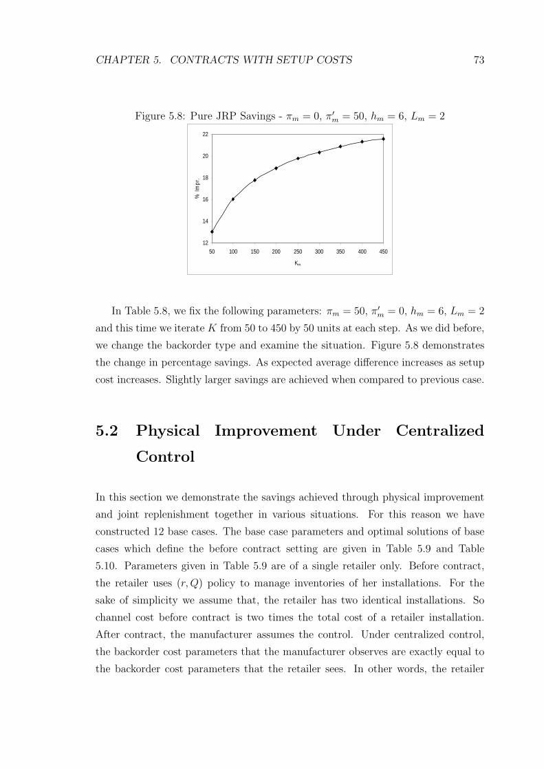
CHAPTER 5. CONTRACTS WITH SETUP COSTS 73
Figure 5.8: Pure JRP Savings - πm = 0, π′m = 50, hm = 6, Lm = 2
12
14
16
18
20
22
50 100 150 200 250 300 350 400 450
Km
% Im
pr.
In Table 5.8, we fix the following parameters: πm = 50, π′m = 0, hm = 6, Lm = 2
and this time we iterate K from 50 to 450 by 50 units at each step. As we did before,
we change the backorder type and examine the situation. Figure 5.8 demonstrates
the change in percentage savings. As expected average difference increases as setup
cost increases. Slightly larger savings are achieved when compared to previous case.
5.2 Physical Improvement Under Centralized
Control
In this section we demonstrate the savings achieved through physical improvement
and joint replenishment together in various situations. For this reason we have
constructed 12 base cases. The base case parameters and optimal solutions of base
cases which define the before contract setting are given in Table 5.9 and Table
5.10. Parameters given in Table 5.9 are of a single retailer only. Before contract,
the retailer uses (r,Q) policy to manage inventories of her installations. For the
sake of simplicity we assume that, the retailer has two identical installations. So
channel cost before contract is two times the total cost of a retailer installation.
After contract, the manufacturer assumes the control. Under centralized control,
the backorder cost parameters that the manufacturer observes are exactly equal to
the backorder cost parameters that the retailer sees. In other words, the retailer

CHAPTER 5. CONTRACTS WITH SETUP COSTS 74
truly reflects its own backorder costs under centralized control and the retailer and
the manufacturer act as a single entity. The channel cost after contract simply
equals to the manufacturer’s cost.
Table 5.9: Contracts with Setup - Base Case Parameter Summary
Base Case Lr hr K πr π′r1 2 6 100 50 0
2 2 6 200 50 0
3 2 6 500 50 0
4 2 6 100 100 0
5 2 6 200 100 0
6 2 6 500 100 0
7 2 6 100 0 50
8 2 6 200 0 50
9 2 6 500 0 50
10 2 6 100 0 100
11 2 6 200 0 100
12 2 6 500 0 100
Table 5.10: Contracts with Setup - Base Case Solution SummaryBase Cases Before Contract Cost Components Costs
Case Q r K hr π′r πr Setup Holding BO2 BO1 Retailer Channel
1 15 11 100 6 0 50 33.333 54.500 0 12.323 100.156 200.312
2 21 10 200 6 0 50 47.620 66.596 0 13.540 127.756 255.511
3 32 8 500 6 0 50 78.125 87.962 0 18.244 184.331 368.661
4 15 13 100 6 0 100 33.333 66.159 0 9.013 108.505 217.010
5 20 12 200 6 0 100 50 75.216 0 11.450 136.666 273.332
6 31 11 500 6 0 100 80.645 102.242 0 11.925 194.812 389.624
7 15 9 100 6 50 0 33.333 43.334 11.120 0 87.787 175.574
8 21 8 200 6 50 0 47.620 55.465 12.212 0 115.297 230.595
9 32 6 500 6 50 0 78.125 77.031 16.921 0 172.077 344.153
10 16 10 100 6 100 0 31.250 51.782 13.030 0 96.062 192.124
11 20 10 200 6 100 0 50 63.625 10.424 0 124.049 248.099
12 31 9 500 6 100 0 80.645 90.646 10.761 0 182.052 364.103
As we mentioned before, physical improvement consists of holding cost reduction

CHAPTER 5. CONTRACTS WITH SETUP COSTS 75
and leadtime improvement. We analyze the savings achieved through leadtime re-
duction and joint replenishment in Section 5.2.1, and through holding cost reduction
and joint replenishment, in Section 5.2.2.
5.2.1 Contracts With Setup Cost - Leadtime Improvement
Table 5.11: Contracts with Setup - Leadtime Improvement, πm = 50, π′m = 0,
Case:1,2,3K=100 K=200 K=500
Lm Qm S Total % Impr. Qm S Total % Impr. Qm S Total % Impr.
0.5 19 14 156.068 22.088 28 18 199.254 22.017 40 23 284.370 22.864
0.75 20 16 159.931 20.159 28 19 202.076 20.913 40 24 286.252 22.354
1 20 17 163.480 18.387 29 21 204.644 19.908 40 25 288.265 21.808
1.25 21 19 166.496 16.881 28 22 207.111 18.943 40 27 289.922 21.358
1.5 20 20 169.541 15.362 30 24 209.395 18.049 40 28 291.465 20.940
1.75 21 22 172.265 14.001 29 25 211.543 17.208 40 29 293.152 20.482
2 21 23 174.902 12.685 31 27 213.692 16.367 40 31 294.972 19.988
2.25 22 25 177.276 11.500 30 28 215.581 15.628 40 32 296.261 19.639
2.5 22 26 179.767 10.256 30 29 217.602 14.836 40 33 297.695 19.250
2.75 23 28 181.901 9.191 31 31 219.321 14.164 40 34 299.267 18.823
3 22 29 184.139 8.074 31 32 221.178 13.437 40 36 300.743 18.423
3.25 24 31 186.213 7.038 32 34 222.829 12.791 40 37 301.973 18.089
3.5 23 32 188.178 6.058 31 35 224.505 12.135 40 38 303.340 17.719
3.75 24 34 190.257 5.019 33 37 226.151 11.491 40 39 304.838 17.312
4 24 35 191.999 4.150 32 38 227.659 10.901 40 40 306.462 16.872
Figure 5.9: Contracts with Setup - Leadtime Improvement, πm = 50, π′m = 0
0
5
10
15
20
25
0.5 1.0 1.5 2.0 2.5 3.0 3.5 4.0
Lm
% Im
prov
emen
t
K=100
K=200
K=500

CHAPTER 5. CONTRACTS WITH SETUP COSTS 76
In Table 5.11 we summarize savings obtained from leadtime improvement in base
case 1,2 and 3. We iterate Lm from 0.5 to 4. We present optimal Q and S values
of the system where S is the base stock level of a single retailer installation under
(Q,S) policy. The analysis is done for K = 100, 200, 500 and it is observed that
the most savings are achieved when K = 500. As we have seen before, further
reductions in leadtime through consignment contract result in more savings. An
interesting observation is, even if the manufacturer leadtime is as large as two times
the retailer leadtime, savings are still possible. Results are also demonstrated in
Figure 5.9.
Table 5.12: Contracts with Setup - Leadtime Improvement, πm = 100, π′m = 0K=100 K=200 K=500
Lm Qm S Total % Impr. Qm S Total % Impr. Qm S Total % Impr.
0.5 18 15 168.257 22.466 25 18 213.780 21.787 40 25 303.368 22.138
0.75 19 17 173.363 20.113 26 20 217.764 20.330 40 26 306.580 21.314
1 18 18 178.047 17.955 27 22 221.520 18.956 40 28 309.095 20.668
1.25 19 20 182.145 16.066 26 23 225.111 17.642 40 29 311.627 20.019
1.5 21 22 186.113 14.237 28 25 228.316 16.469 40 30 314.554 19.267
1.75 20 23 189.607 12.628 27 26 231.402 15.340 40 32 316.560 18.753
2 21 25 193.026 11.052 28 28 234.207 14.314 40 33 318.911 18.149
2.25 20 26 196.330 9.530 29 30 237.103 13.255 40 35 321.431 17.502
2.5 21 28 199.401 8.114 29 31 239.788 12.272 40 36 323.297 17.023
2.75 20 29 202.569 6.654 30 33 242.371 11.327 40 37 325.497 16.459
3 22 31 205.305 5.394 29 34 244.750 10.457 40 39 327.722 15.888
3.25 21 32 208.096 4.108 30 36 247.277 9.532 40 40 329.483 15.436
3.5 22 34 210.677 2.918 30 37 249.528 8.709 39 40 333.374 14.437
3.75 21 35 213.394 1.666 29 38 251.817 7.871 36 40 339.256 12.927
4 23 37 215.829 0.544 30 40 253.961 7.087 34 40 347.045 10.928

CHAPTER 5. CONTRACTS WITH SETUP COSTS 77
Figure 5.10: Contracts with Setup - Leadtime Improvement, πm = 100, π′m = 0
0
5
10
15
20
25
30
0.5 1.0 1.5 2.0 2.5 3.0 3.5 4.0
Lm
% Im
prov
emen
t
K=100
K=200
K=500
In Table 5.12 we summarize savings obtained from leadtime improvement in base
case 4,5 and 6. The difference between these base cases and previous ones is the
greater backorder. Again we iterate Lm from 0.5 to 4. Same results with the previous
cases are obtained. However with larger backorder costs, the savings diminish faster
as it can be observed in Figure 5.10.
Table 5.13: Contracts with Setup - Leadtime Improvement, πm = 0, πm′ = 50K=100 K=200 K=500
Lm Qm S Total % Impr. Qm S Total % Impr. Qm S Total % Impr.
0.5 20 12 127.986 27.104 27 15 170.701 25.974 40 21 256.736 25.401
0.75 19 13 131.764 24.952 28 17 173.753 24.650 40 22 258.907 24.770
1 20 15 135.167 23.014 28 18 176.683 23.379 40 23 261.447 24.032
1.25 21 17 138.611 21.053 29 20 179.356 22.220 40 25 263.500 23.435
1.5 21 18 141.556 19.375 28 21 181.982 21.082 40 26 265.571 22.834
1.75 22 20 144.596 17.644 29 23 184.569 19.960 40 27 267.993 22.130
2 21 21 147.385 16.055 29 24 187.037 18.889 40 29 269.806 21.603
2.25 22 23 150.266 14.415 30 26 189.406 17.862 40 30 271.800 21.023
2.5 22 24 152.845 12.945 29 27 191.728 16.855 40 31 274.130 20.347
2.75 23 26 155.491 11.438 30 29 194.101 15.826 40 33 275.749 19.876
3 22 27 157.911 10.060 30 30 196.195 14.918 40 34 277.682 19.314
3.25 23 29 160.523 8.572 31 32 198.439 13.945 40 36 279.823 18.692
3.5 23 30 162.760 7.298 30 33 200.522 13.041 40 37 281.397 18.235
3.75 22 31 165.138 5.944 30 34 202.616 12.133 40 38 283.275 17.689
4 23 33 167.359 4.679 31 36 204.585 11.279 40 40 285.258 17.113
In Table 5.13 we summarize savings obtained from leadtime improvement in base

CHAPTER 5. CONTRACTS WITH SETUP COSTS 78
Figure 5.11: Contracts with Setup - Leadtime Improvement, πm = 0, π′m = 50
10
15
20
25
30
35
40
45
3.0 3.5 4.0 4.5 5.0 5.5 6.0
hm
% Im
prov
emen
t
K=100
K=200
K=500
case 7,8 and 9. For these base cases, we have type II backorder costs, as opposed
to type I backorder costs in the previous cases. Again we iterate Lm from 0.5 to 4.
Same results with the previous cases are obtained. Results can be observed in 5.11.
Table 5.14: Contracts with Setup - Leadtime Improvement, πm = 0, π′m = 100K=100 K=200 K=500
Lm Qm S Total % Impr. Qm S Total % Impr. Qm S Total % Impr.
0.5 19 13 140.213 27.019 26 16 184.911 25.469 39 22 274.469 24.618
0.75 18 14 144.983 24.536 27 18 188.864 23.875 40 24 277.227 23.860
1 19 16 149.249 22.316 26 19 192.605 22.368 40 25 280.510 22.959
1.25 20 18 153.404 20.153 27 21 196.074 20.969 40 27 283.096 22.248
1.5 19 19 157.317 18.117 28 23 199.542 19.571 40 28 285.861 21.489
1.75 20 21 160.968 16.217 28 24 202.750 18.279 40 30 288.756 20.694
2 20 22 164.460 14.399 29 26 205.862 17.024 40 31 291.074 20.057
2.25 21 24 167.736 12.694 28 27 208.729 15.869 40 32 293.934 19.272
2.5 20 25 171.091 10.947 29 29 211.661 14.687 40 34 296.192 18.652
2.75 21 27 174.098 9.382 28 30 214.458 13.559 40 35 298.616 17.986
3 22 29 177.268 7.732 29 32 217.263 12.429 40 37 301.245 17.264
3.25 21 30 180.159 6.228 29 33 219.916 11.360 40 38 303.281 16.705
3.5 22 32 183.172 4.659 30 35 222.522 10.309 40 39 305.788 16.016
3.75 22 33 185.843 3.269 29 36 224.993 9.313 39 40 308.678 15.222
4 23 35 188.667 1.799 30 38 227.556 8.280 37 40 313.957 13.772
In Table 5.14 we summarize savings obtained from leadtime improvement in base
case 10,11 and 12. The difference between these base cases and previous ones is the
greater backorder cost. Again we iterate Lm from 0.5 to 4. Same results with the
previous cases are obtained. Results can be observed in Figure 5.12. Considering

CHAPTER 5. CONTRACTS WITH SETUP COSTS 79
Figure 5.12: Contracts with Setup - Leadtime Improvement, πm = 0, π′m = 100
12
17
22
27
32
37
42
3.0 3.5 4.0 4.5 5.0 5.5 6.0
hm
% Im
prov
emen
t
K=100
K=200
K=500
all base cases, greater savings are obtained from leadtime improvement and joint
replenishment when K = 500. Another common observation is, savings percentage
diminish faster under high backorder cost.
5.2.2 Contracts With Setup Cost - Holding cost improve-
ment
Table 5.15: Contracts with Setup - Holding Cost Improvement, πm = 50, π′m = 0K=100 K=200 K=500
hm Q S Total % Impr. Q S Total % Impr. Q S Total % Impr.
3 28 28 117.104 41.539 39 33 146.943 42.491 40 33 221.956 39.794
3.25 26 27 122.747 38.722 38 32 153.441 39.948 40 33 228.613 37.988
3.5 27 27 128.087 36.056 36 31 159.765 37.472 40 33 235.270 36.183
3.75 25 26 133.313 33.447 36 31 165.923 35.062 40 32 241.768 34.420
4 25 26 138.341 30.937 35 30 171.752 32.781 40 32 247.943 32.745
4.25 25 26 143.369 28.427 33 29 177.522 30.523 40 32 254.117 31.070
4.5 24 25 148.140 26.045 33 29 183.064 28.354 40 32 260.291 29.396
4.75 24 25 152.802 23.718 32 28 188.553 26.206 40 32 266.465 27.721
5 24 25 157.464 21.391 32 28 193.731 24.179 40 31 272.179 26.171
5.25 22 24 161.919 19.166 32 28 198.909 22.153 40 31 277.878 24.625
5.5 22 24 166.332 16.963 30 27 203.938 20.185 40 31 283.576 23.080
5.75 23 24 170.669 14.798 30 27 208.867 18.255 40 31 289.274 21.534
6 21 23 174.902 12.685 31 27 213.692 16.367 40 31 294.972 19.988

CHAPTER 5. CONTRACTS WITH SETUP COSTS 80
Figure 5.13: Contracts with Setup - Holding Cost Improvement, πm = 50, π′m = 0
0
5
10
15
20
25
0.5 1.0 1.5 2.0 2.5 3.0 3.5 4.0
Lm
% Im
prov
emen
t
K=100
K=200
K=500
In Table 5.15 we summarize savings obtained from leadtime improvement in base
case 1,2 and 3. We iterate hm from 3 to 6. We present optimal Q and S values of the
system where S is the base stock level of a single retailer installation under (Q,S)
policy. The analysis is done for K = 100, 200, 500 and it is observed that the most
remarkable savings are achieved when K = 200 but we should note that savings are
very close for all setup costs. As we have seen before, reduction in leadtime results
in further savings. Improving holding cost to 3 from 6 brings around 40% savings
in all setup costs. Results are also demonstrated in Figure 5.13.
Table 5.16: Contracts with Setup - Holding Cost Improvement, πm = 100, π′m = 0K=100 K=200 K=500
h Qm S Total % Impr. Qm S Total % Impr. Qm S Total % Impr.
3 26 29 126.008 41.934 37 34 156.944 42.581 40 35 232.238 40.394
3.25 27 29 132.313 39.029 36 33 164.390 39.857 40 35 239.875 38.434
3.5 25 28 138.397 36.225 36 33 171.528 37.246 40 35 247.513 36.474
3.75 25 28 144.407 33.456 34 32 178.459 34.710 40 35 255.150 34.514
4 23 27 150.331 30.726 32 31 185.338 32.193 40 34 262.748 32.564
4.25 24 27 156.006 28.111 33 31 191.891 29.796 40 34 269.893 30.730
4.5 22 26 161.635 25.517 31 30 198.315 27.446 40 34 277.038 28.896
4.75 22 26 167.023 23.034 31 30 204.581 25.153 40 34 284.184 27.062
5 22 26 172.411 20.552 31 30 210.847 22.860 40 34 291.329 25.228
5.25 22 26 177.799 18.069 29 29 216.884 20.652 40 34 298.474 23.394
5.5 21 25 182.991 15.676 30 29 222.792 18.490 40 33 305.597 21.566
5.75 21 25 188.008 13.364 28 28 228.561 16.380 40 33 312.254 19.858
6 21 25 193.026 11.052 28 28 234.207 14.314 40 33 318.911 18.149

CHAPTER 5. CONTRACTS WITH SETUP COSTS 81
Figure 5.14: Contracts with Setup - Holding Cost Improvement, πm = 100, π′m = 0
0
5
10
15
20
25
30
0.5 1.0 1.5 2.0 2.5 3.0 3.5 4.0
Lm
% Im
prov
emen
t
K=100
K=200
K=500
In Table 5.16 we summarize savings obtained from leadtime improvement in base
case 4,5 and 6. We iterate hm from 3 to 6. Similar results are found as previous
cases. Results are also demonstrated in Figure 5.14.
Table 5.17: Contracts with Setup - Holding Cost Improvement, πm = 0, π′m = 50K=100 K=200 K=500
hm Qm S Total % Impr. Qm S Total % Impr. Qm S Total % Impr.
3 29 26 102.931 41.375 38 30 132.984 42.330 40 31 208.037 39.551
3.25 27 25 107.275 38.900 38 30 138.434 39.967 40 31 213.735 37.895
3.5 27 25 111.595 36.440 36 29 143.664 37.699 40 31 219.434 36.240
3.75 25 24 115.687 34.109 35 28 148.626 35.547 40 30 224.773 34.688
4 26 24 119.664 31.844 35 28 153.470 33.446 40 30 230.005 33.168
4.25 24 23 123.410 29.710 33 27 158.109 31.434 40 30 235.236 31.648
4.5 24 23 127.128 27.593 33 27 162.706 29.441 40 30 240.468 30.128
4.75 24 23 130.845 25.475 32 26 166.978 27.588 40 30 245.699 28.608
5 23 22 134.312 23.501 32 26 171.222 25.748 40 29 250.702 27.154
5.25 23 22 137.679 21.583 30 25 175.322 23.970 40 29 255.478 25.766
5.5 23 22 141.046 19.665 30 25 179.320 22.236 40 29 260.254 24.379
5.75 21 21 144.262 17.834 30 25 183.319 20.502 40 29 265.030 22.991
6 21 21 147.385 16.055 29 24 187.037 18.889 40 29 269.806 21.603

CHAPTER 5. CONTRACTS WITH SETUP COSTS 82
Figure 5.15: Contracts with Setup - Holding Cost Improvement, πm = 0, π′m = 50
10
15
20
25
30
35
40
45
3.0 3.5 4.0 4.5 5.0 5.5 6.0
hm
% Im
prov
emen
t
K=100
K=200
K=500
In Table 5.17 we summarize savings obtained from leadtime improvement in base
case 7,8 and 9. We iterate hm from 3 to 6. Similar results are found as previous
cases. Results are also demonstrated in Figure 5.15.
Table 5.18: Contracts with Setup - Holding Cost Improvement, πm = 0, π′m = 100K=100 K=200 K=500
hm Qm S Total % Impr. Qm S Total % Impr. Qm S Total % Impr.
3 27 27 111.407 42.013 38 32 142.463 42.578 40 33 217.709 40.207
3.25 26 26 116.591 39.314 36 31 148.688 40.069 40 33 224.366 38.379
3.5 26 26 121.502 36.758 35 30 154.691 37.650 40 33 231.023 36.550
3.75 24 25 126.288 34.267 35 30 160.482 35.315 40 32 237.265 34.836
4 24 25 130.950 31.841 33 29 166.027 33.080 40 32 243.439 33.140
4.25 24 25 135.612 29.414 31 28 171.568 30.847 40 32 249.613 31.444
4.5 23 24 139.919 27.173 32 28 176.805 28.736 40 32 255.787 29.749
4.75 23 24 144.216 24.936 30 27 181.930 26.671 40 32 261.962 28.053
5 21 23 148.475 22.719 30 27 186.859 24.684 40 32 268.136 26.357
5.25 21 23 152.525 20.611 30 27 191.788 22.697 40 31 273.979 24.752
5.5 21 23 156.574 18.503 28 26 196.602 20.757 40 31 279.677 23.187
5.75 21 23 160.624 16.395 28 26 201.283 18.870 40 31 285.376 21.622
6 20 22 164.460 14.399 29 26 205.862 17.024 40 31 291.074 20.057

CHAPTER 5. CONTRACTS WITH SETUP COSTS 83
Figure 5.16: Contracts with Setup - Holding Cost Improvement, πm = 0, π′m = 100
15
20
25
30
35
40
45
3.0 3.5 4.0 4.5 5.0 5.5 6.0
hm
% Im
prov
emen
t
K=100
K=200
K=500
In Table 5.18 we summarize savings obtained from leadtime improvement in base
case 10,11 and 12. We iterate hm from 3 to 6. Similar results are found as previous
cases. Results are also demonstrated in Figure 5.16.
Similar to our study in Section 4.1, we compared the effects of leadtime reduction
and holding cost reduction. In our data sets, again holding cost reduction brought
more savings than leadtime improvement. As holding cost is reduced, inventory
levels increase while cost of holding such large inventories decrease which in turn
reduces the backorders due to decreased number of stockouts. Similar to what we
have found in Section 4.1 as base stock levels decrease due to shorter leadtime, the
backorders may increase and hamper the savings.
5.3 Decentralized Control
In this section, we analyze the effect of retailer charging different backorder costs
than what she observes on supply chain costs when manufacturer utilizes joint re-
plenishment without providing physical improvement. As we defined in Chapter 3,
the retailer observes πr and π′r but in the contract she may charge the manufacturer
backorder costs which are different (i.e. πm 6= πr and π′m 6= π′r). This manipulation
can be done in various ways. First the amount the backorder cost may be changed

CHAPTER 5. CONTRACTS WITH SETUP COSTS 84
without changing the type of backorder. For example, if retailer is charged per oc-
casion basis by customer, she may charge the manufacturer on per occasion basis
but with a larger cost. Second, the retailer may charge a different type of backorder
cost (possibly with a different amount than what she faces) to manufacturer, such
as incurring Type II backorder cost while facing Type I backorder cost. Again we
define 12 base cases to demonstrate the behavior of cost functions of the retailer,
the manufacturer and the supply chain. The base case initial parameters for a single
retailer and backorder cost ranges that are incurred to manufacturer are given in
the Table 5.19. The optimal solution of base cases before contract are given in Table
5.20.
Table 5.19: Contracts with Setup, Decentralized Control - Base Case Parameter
SummaryRetailer Manufacturer
Base Case Lr hr K πr π′r Lm hm K πm π′m1 2 6 100 0 100 2 6 100 0 [10, 150]
2 2 6 200 0 100 2 6 200 0 [10, 150]
3 2 6 500 0 100 2 6 500 0 [10, 150]
4 2 6 100 0 50 2 6 100 0 [25, 75]
5 2 6 200 0 50 2 6 200 0 [25, 75]
6 2 6 500 0 50 2 6 500 0 [25, 75]
7 2 6 100 50 0 2 6 100 [25, 75] 0
8 2 6 200 50 0 2 6 200 [25, 75] 0
9 2 6 500 50 0 2 6 500 [25, 75] 0
10 2 6 100 0 50 2 6 100 [25, 75] 0
11 2 6 200 0 50 2 6 200 [25, 75] 0
12 2 6 500 0 50 2 6 500 [25, 75] 0

CHAPTER 5. CONTRACTS WITH SETUP COSTS 85
Table 5.20: Contracts with Setup, Decentralized Control - Base Case Solution Sum-
maryRetailer’s Optimal Parameters Cost Components Costs
Case Qr rr K hr πr π′r Setup Holding BO1 BO2 Single Ret Channel Cost
1 16 10 100 6 0 100 62.500 103.564 0 26.060 96.062 192.124
2 20 10 200 6 0 100 100 127.251 0 20.848 124.049 248.099
3 31 9 500 6 0 100 161.290 181.291 0 21.522 182.052 364.103
4 15 9 100 6 0 50 66.666 86.669 0 22.239 87.787 175.574
5 21 8 200 6 0 50 95.240 110.931 0 24.424 115.297 230.595
6 32 6 500 6 0 50 156.250 154.061 0 33.842 172.077 344.153
7 15 11 100 6 50 0 66.666 109.001 24.645 0 100.156 200.312
8 21 10 200 6 50 0 95.240 133.191 27.080 0 127.756 255.511
9 32 8 500 6 50 0 156.250 175.923 36.488 0 184.331 368.661
10 15 9 100 6 0 50 66.666 86.669 0 22.239 87.787 175.574
11 21 8 200 6 0 50 95.240 110.931 0 24.424 115.297 230.595
12 32 6 500 6 0 50 156.250 154.061 0 33.842 172.077 344.153
Table 5.21: Contracts with Setup, Decentralized Control, πm = 0, π′m = 10 : 150,
Case: 1, 2, 3
K=100 K=200 K=500
π′m MFG RET CHN % IMPR. MFG RET CHN % IMPR. MFG RET CHN % IMPR.
10 103.41 247.21 350.63 -82.500 136.48 318.68 455.16 -83.460 212.63 341.07 553.70 -52.073
20 122.97 115.38 238.35 -24.061 159.35 125.65 285 -14.872 238.35 154.92 393.27 -8.011
30 134.02 61.38 195.40 -1.705 171.97 70.59 242.56 2.231 252.64 79.03 331.67 8.907
40 141.74 35.58 177.32 7.705 180.57 42.91 223.48 9.924 262.41 50.10 312.52 14.168
50 147.39 24.79 172.18 10.382 187.04 30.42 217.46 12.350 269.81 30.18 299.99 17.609
60 152.11 16.43 168.54 12.277 192.24 16.53 208.76 15.855 275.84 24.15 299.99 17.609
70 155.86 9.57 165.43 13.893 196.37 12.40 208.76 15.855 280.38 12.78 293.16 19.485
80 159.05 6.38 165.43 13.893 199.89 6.85 206.75 16.668 284.64 8.52 293.16 19.485
90 161.87 2.59 164.46 14.399 203.09 2.81 205.91 17.005 288.14 2.93 291.07 20.057
100 164.46 0 164.46 14.399 205.86 0 205.86 17.024 291.07 0 291.07 20.057
110 166.66 -1.99 164.67 14.288 208.18 -2.22 205.96 16.983 294.01 -2.93 291.07 20.057
120 168.65 -3.97 164.67 14.288 210.40 -4.44 205.96 16.983 296.76 -3.93 292.83 19.574
130 170.49 -4.74 165.75 13.727 212.42 -5.37 207.05 16.544 298.73 -5.90 292.83 19.574
140 172.07 -6.32 165.75 13.727 214.22 -7.16 207.05 16.544 300.69 -7.86 292.83 19.574
150 173.65 -7.90 165.75 13.727 216.01 -8.95 207.05 16.544 302.66 -9.83 292.83 19.574
In Table 5.21, we present the costs of the manufacturer, the retailer and the
channel in base case 1, 2 and 3, after contract. Again note that the cost figures for
the retailer and the manufacturer exclude the annual payment A. Note that setup
cost is the only parameter that distinguishes these base cases. Type II backorder
cost incurred by retailer, π′m, is iterated between 10 and 150 by units of 10. It is
observed that when the retailer charges a backorder cost that is too low, channel
suffers since the manufacturer keeps insufficient inventory. Minimum channel cost
and maximum percentage savings are achieved in intervals around original Type II
backorder cost, 100. When compared to the results we observed in Chapter 4, here

CHAPTER 5. CONTRACTS WITH SETUP COSTS 86
intervals are much more narrow. Greatest percentage savings are achieved under
K = 500. The percentage savings are depicted in Figure 5.17. In Figure 5.18, the
costs of manufacturer, retailer and channel in base case 1 are depicted.
Figure 5.17: Contracts with Setup, Decentralized Control, πm = 0, π′m = 10 : 150,
Case: 1, 2, 3
10
12
14
16
18
20
50 70 90 110 130 150m'
% Im
prov
emen
t
K=100
K=200
K=500
Figure 5.18: Contracts with Setup, Decentralized Control, πm = 0, π′m = 10 : 150,
Case 1 Costs
-10
40
90
140
190
50 70 90 110 130 150m'
Cos
ts
MFG
RET
CHN
INITIAL

CHAPTER 5. CONTRACTS WITH SETUP COSTS 87
Table 5.22: Contracts with Setup, Decentralized Control, πm = 0, π′m = 25 : 75,
Case:4, 5, 6
K=100 K=200 K=500
π′m MFG RET CHN % IMPR. MFG RET CHN % IMPR. MFG RET CHN % IMPR.
25 129.14 25.54 154.68 11.899 166.43 28.97 195.40 15.262 246.30 37.34 283.65 17.581
30 134.02 17.54 151.56 13.678 171.97 20.17 192.14 16.676 252.64 22.58 275.22 20.029
35 138.23 11.20 149.43 14.893 176.69 13.07 189.76 17.709 258.24 12.53 270.76 21.325
40 141.74 5.93 147.67 15.895 180.57 7.15 187.72 18.594 262.41 8.35 270.76 21.325
45 144.70 2.97 147.67 15.895 183.99 3.04 187.04 18.889 266.59 4.18 270.76 21.325
50 147.39 0 147.39 16.055 187.04 0 187.04 18.889 269.81 0 269.81 21.603
55 149.86 -2.48 147.39 16.055 189.74 -2.57 187.17 18.832 272.82 -3.02 269.81 21.603
60 152.11 -4.11 148 15.704 192.24 -4.13 188.10 18.427 275.84 -6.04 269.81 21.603
65 154.07 -5.83 148.24 15.571 194.30 -6.20 188.10 18.427 278.25 -6.39 271.86 21.007
70 155.86 -6.38 149.48 14.861 196.37 -8.26 188.10 18.427 280.38 -8.52 271.86 21.007
75 157.46 -7.97 149.48 14.861 198.18 -8.57 189.62 17.771 282.51 -10.65 271.86 21.007
In Table ??, we present the costs of the manufacturer, the retailer and channel
in base case 4, 5 and 6, after contract. Type II backorder cost incurred by retailer,
π′m, is iterated between 25 and 75 by units of 5. Different from previous cases,
backorder costs are lower. Minimum channel cost and maximum percentage savings
are achieved in intervals around original Type II backorder cost, 50. Again, greatest
percentage savings are achieved under K = 500. The percentage savings are shown
in Figure 5.19. In Figure 5.20, the costs of the manufacturer, the retailer and the
channel in base case 4 are depicted.
Figure 5.19: Contracts with Setup, Decentralized Control, πm = 0, π′m = 25 : 75,
Case:4, 5, 6
10
12
14
16
18
20
22
24
25 35 45 55 65 75m'
% Im
prov
emen
t
K=100
K=200
K=500

CHAPTER 5. CONTRACTS WITH SETUP COSTS 88
Figure 5.20: Contracts with Setup, Decentralized Control, πm = 0, π′m = 25 : 75,
Case 3 Costs
-20
20
60
100
140
180
25 35 45 55 65 75m'
Cos
tsMFG
RET
CHN
INITIAL
Table 5.23: Contracts with Setup, Decentralized Control, πm = 25 : 75, π′m = 0,
Case:7, 8, 9
K=100 K=200 K=500
πm MFG RET CHN % IMPR. MFG RET CHN % IMPR. MFG RET CHN % IMPR.
25 153.10 33.06 186.15 7.068 187.68 42.29 229.97 9.997 264.32 55.35 319.67 13.289
30 159.31 23.34 182.65 8.818 195.31 27.79 223.09 12.688 273.10 29.39 302.49 17.949
35 164.27 12.41 176.68 11.798 201.21 15.79 217 15.070 280.12 17.35 297.47 19.311
40 168.31 7.09 175.40 12.434 206.05 9.28 215.33 15.725 285.90 11.57 297.47 19.311
45 171.86 3.55 175.40 12.434 210.17 4.06 214.23 16.155 290.53 4.44 294.97 19.988
50 174.90 0 174.90 12.685 213.69 0 213.69 16.367 294.97 0 294.97 19.988
55 177.54 -2.38 175.16 12.557 216.68 -2.88 213.80 16.326 298.29 -3.32 294.97 19.988
60 179.92 -4.76 175.16 12.557 219.42 -4.90 214.52 16.042 301.62 -6.64 294.97 19.988
65 182.01 -5.93 176.09 12.093 221.88 -7.35 214.52 16.042 304.58 -7.25 297.34 19.347
70 183.99 -7.90 176.09 12.093 224.13 -8.25 215.89 15.509 307 -9.66 297.34 19.347
75 185.88 -8.11 177.77 11.252 226.20 -10.31 215.89 15.509 309.41 -12.08 297.34 19.347
In Table 5.23, we present the costs of the manufacturer, the retailer and channel
in base case 7, 8 and 9, after contract. Type I backorder cost incurred by retailer,
πm,is iterated between 25 and 75 by units of 5. The difference from previous cases
is, now backorder cost type is different. Minimum channel cost and maximum
percentage savings are achieved in intervals around original Type I backorder cost,
50. Again, greatest percentage savings are achieved under K = 500. The percentage
savings are shown in Figure 5.21. In Figure 5.22, the costs of the manufacturer, the
retailer and the channel in base case 7 are depicted.

CHAPTER 5. CONTRACTS WITH SETUP COSTS 89
Figure 5.21: Contracts with Setup, Decentralized Control,πm = 25 : 75, π′m = 0,
Case:7, 8, 9
6
8
10
12
14
16
18
20
25 35 45 55 65 75m
% Im
prov
emen
tK=100
K=200
K=500
Figure 5.22: Contracts with Setup, Decentralized Control, πm = 25 : 75, π′m = 0,
Case 7 Costs
-15
35
85
135
185
25 35 45 55 65 75m
Cos
ts
MFG
RET
CHN
INITIAL

CHAPTER 5. CONTRACTS WITH SETUP COSTS 90
Table 5.24: Contracts with Setup, Decentralized Control, πm = 25 : 75, π′m = 0,
Case:10, 11, 12
K=100 K=200 K=500
πm MFG RET CHN % IMPR. MFG RET CHN % IMPR. MFG RET CHN % IMPR.
25 153.10 -4.96 148.14 15.625 187.68 4.06 191.74 16.851 264.32 19.33 283.65 17.581
30 159.31 -11.53 147.78 15.830 195.31 -7.31 187.99 18.476 273.10 -2.33 270.76 21.325
35 164.27 -13.75 150.51 14.274 201.21 -13.01 188.20 18.385 280.12 -10.31 269.81 21.603
40 168.31 -16.02 152.29 13.261 206.05 -17.17 188.88 18.092 285.90 -16.10 269.81 21.603
45 171.86 -19.57 152.29 13.261 210.17 -19.95 190.23 17.506 290.53 -18.67 271.86 21.007
50 174.90 -20.16 154.74 11.865 213.69 -20.34 193.35 16.150 294.97 -18.56 276.42 19.682
55 177.54 -18.58 158.96 9.462 216.68 -20.91 195.77 15.103 298.29 -21.88 276.42 19.682
60 179.92 -20.95 158.96 9.462 219.42 -20.68 198.74 13.814 301.62 -25.20 276.42 19.682
65 182.01 -19.70 162.32 7.550 221.88 -23.13 198.74 13.814 304.58 -21.58 283.01 17.767
70 183.99 -21.67 162.32 7.550 224.13 -21.89 202.24 12.295 307 -23.99 283.01 17.767
75 185.88 -19.66 166.22 5.329 226.20 -23.95 202.24 12.295 309.41 -26.41 283.01 17.767
In Table 5.24, we present the costs of the manufacturer, the retailer and channel
in base case 10, 11 and 12, after contract. Different from previous cases, the retailer
charges a different backorder cost type. The retailer faces backorders in per unit per
time basis, but charges the manufacturer in per occasion basis. Minimum channel
cost and maximum percentage savings are achieved in intervals around 30 for all
cases. This is similar to our findings in Chapter 4. Again, greatest percentage
savings are achieved under K = 500. The percentage savings are shown in Figure
5.23. In Figure 5.24, the costs of the manufacturer, the retailer and the channel in
base case 10 are depicted.
Figure 5.23: Contracts with Setup, Decentralized Control, πm = 25 : 75, π′m = 0,
Case:10, 11, 12
0
5
10
15
20
25
25 35 45 55 65 75m
% Im
prov
emen
t
K=100
K=200
K=500

CHAPTER 5. CONTRACTS WITH SETUP COSTS 91
Figure 5.24: Contracts with Setup, Decentralized Control, πm = 25 : 75, π′m = 0,
Case 10 Costs
-25
25
75
125
175
25 35 45 55 65 75m
Cos
tsMFG
RET
CHN
INITIAL

Chapter 6
Conclusion
In this thesis, we consider a spare parts inventory system. In this system, the
manufacturer provides spare parts of a capital equipment to its customers. The
manufacturer and its customers agree to a full service Vendor Managed Inventory
(VMI) contract to coordinate their activities and exploit the benefits of VMI. The
specific contract we will consider is a consignment contract, under which the man-
ufacturer assumes the responsibility and the ownership of the inventory in a stock
room inside the facilities of its customers. In exchange for this service, the customers
pay an annual fee.
In the setting we consider, moving the control from the customer to the manufac-
turer can provide system improvements such as lower cost of inventory ownership,
shorter leadtime and the ability to jointly replenish multiple installations. We first
use basic inventory models to quantify the savings obtained through these improve-
ments. For the case of no setup costs, the customers before the contract and the
manufacturer after the contract use a simple base stock policy. For the case of
setup costs, the customers before the contract use independent (r,Q) policy at each
installation and the manufacturer after the contract uses a (Q,S) policy to jointly
manage multiple installations.
There can be various types of contracts which are structured using different
terms. Service levels, inventory levels and backorder costs are some examples of
92

CHAPTER 6. CONCLUSION 93
possible terms on which the contract can be structured. We structure our contract
on backorder costs (π, π′) and the annual payment of the delegating party. Using the
cost expressions that are introduced in beforehand mentioned models, we conduct
a numerical study to demonstrate the savings that are achieved through leadtime
and holding cost reduction in a setting without setup costs. It is observed that
both leadtime reduction and holding cost reduction are considerably effective. We
then examine the impact of the retailer charging backorder costs that are differ-
ent from what she observes. We show numerically that, if the retailer manipulates
backorder penalties, the supply chain efficiency will suffer, and in fact, the supply
chain costs may be higher than before the contract even if there are physical im-
provements mentioned above. We repeat the same analysis for the case of positive
setup costs for which similar results are obtained. We also demonstrate the effect
of joint replenishment alone by comparing the total costs obtained from (r,Q) and
(Q,S) policies. Joint replenishment brings savings in all cases and the savings are
the most remarkable under high setup costs. It is also found that as per unit back-
order costs increase, the savings through joint replenishment diminish. In our data
sets, holding cost reduction brought more savings than leadtime improvement. As
holding cost is reduced, inventory levels increase while cost of holding such large
inventories decrease which in turn reduces the backorders due to decreased number
of stockouts. But in leadtime reduction case, as base stock levels decrease due to
shorter leadtime, the backorders may increase and hamper the savings.
We note that the primary difference between our study and earlier research is
that we extend the consignment contracts literature in the direction of joint replen-
ishment. We use backorder costs and the annual fee as the terms of the contract and
search for values of these variables which coordinate the supply chain. In this re-
search, we use leadtime reduction, holding cost reduction and joint replenishment to
create savings in a spare parts consignment contract. However, to our knowledge our
study is the first to simultaneously consider these concepts. Our numerical results
indicate that simultaneous usage of physical improvement and joint replenishment
indeed results in significant inventory and cost savings.
Future research can extend the analysis here in many directions. A natural ques-
tion to consider is how to allocate those savings to the parties in the supply chain.

CHAPTER 6. CONCLUSION 94
In our models, we state that the customers pay an annual fee to the manufacturer
for the consignment service. However, we did not elaborate on how to determine this
fee, except for giving a range. To specify the exact amount of this fee, bargaining
models can be used. Another extension may include quantifying the cost of manu-
facturer’s effort to reduce its leadtime. A further extension could be to use different
joint replenishment policies such as (S, c, s) policy. Finally, our numerical results
could be strengthened by using more than two installation that are non–identical.

Bibliography
[1] Applied Materials Inc. Amat annual report. www.supplychainonline.com,
2004.
[2] B. Arnold. E-commerce, increasing device complexity offer new twists in value-
added service support. Semiconductor Magazine, 1(4), 2000.
[3] A. Aschner. The Gower Handbook of Logistics and Distribution management,
chapter Managing and Controlling Logistics Inventories. Aldershot: Gower,
Brookfield, 1990.
[4] D. R. Atkins and P. O. Iyogun. Periodic versus can-orderpolicies for coordinated
multi-item inventory systems. Management Science, (34):791–796, 1988.
[5] S. Axster. Inventory Control. Kluwer, Boston, 2000.
[6] K. R. Baker. Lot-sizing procedures and a standard data set: A reconcilation of
the literature. Journal of Manufacturing and Operations Management, (2):199–
221, 1998.
[7] J. L. Balintfy. On a basic class of multi-item inventory problems. Management
Science, (10):287–297, 1964.
[8] M. Bastian. Joint replenishment in multi-item inventory systems. Journal of
the Operational Research Society, (37):1113–1120, 1986.
[9] G. P. Cachon. Managing a retailers shelf space, inventory, and transporta-
tion. MANUFACTURING and SERVICE OPERATIONS MANAGEMENT,
3(3):211229, 2001.
95

BIBLIOGRAPHY 96
[10] G. P. Cachon. Supply Chain Management: Design, Coordination and Opera-
tion, volume 11 of Handbooks in Operations Research and Management Science,
chapter 6, Supply Chain Coordination with Contracts, pages 229–332. Elsevier,
Amsterdam, Netherlands, 2003.
[11] H. Canaday. Oems in mro. Overhaul and Maintenance, VII(8), 2001.
[12] S. Cetinkaya and C. Lee. Stock replenishment and shipment scheduling for
vendor managed inventory systems. Management Science, 46:217–232, 2000.
[13] A. K. Chakravarty. Multi-item inventory aggregation into groups. Journal of
the Operational Research Society, (32):19–26, 1981.
[14] A. K. Chakravarty. An optimal heuristic for coordinated multi-item inventory
replenishements. Journal of the Operational Research Society, (36):1027–1039,
1985.
[15] B. A. Chaouch. Stock levels and delivery rates in vendor-managed inventory
programs. Production and Operations Management, 10(1):31–44, 2001.
[16] K. L. Cheung and H. L. Lee. The inventory benefit of shipment coordination
and stock rebalancing in supply chain. Management Science, 48:300–306, 2002.
[17] K. Choi, J. G. Dai, and J. Song. On measuring supplier performance under
vendor-managed-inventory programs in capacitated supply chains. Manufac-
turing and Service Operations Management, 6(1):53–72, 2004.
[18] M. Christopher. Logistics and Supply Chain Management. Financial
Times/Prentice Hall, 1998.
[19] J. Corbett. Stochastic inventory systems in a supply chain with symmetric
information: Cycle stocks, safety stocks and consignment stock. Operations
Research, 49(4):487–500, 2001.
[20] J. Corbett, J. D. Blackburn, and L. N. V. Wassenhove. Case study: Partner-
ships to improve supply chains. Sloan Management Review, 1999.

BIBLIOGRAPHY 97
[21] A. Federgruen, H. Groenevelt, and H. C. Tijms. Coordinated replenishments in
a multi-item inventory system with compound poisson demand. Management
Science, (30):344–357, 1984.
[22] M. J. Fry, R. Kapuscinski, and T. L. Olsen. Coordinating production and
delivery under a (z,z)-type vendor-managed inventory contract. Manufacturing
and Service Operations Management, 3(2):151–173, 2001.
[23] Y. Fu and R. Piplani. Supply side colloboration and its value in supply chains.
European Journal of Operational Research, 152:281–288, 2004.
[24] S. K. Goyal. Determination of economic packaging frequency of items jointly
replenished. Management Science, (20):232–235, 1934.
[25] S. K. Goyal. Determination of optimal packaging frequency of jointly replen-
ished items. Management Science, (21):436–443, 1974.
[26] S. K. Goyal. Optimum ordering policy for a multi-item single supplier system.
Operational Research Quarterly, (25):293–298, 1974.
[27] S. C. Graves. On the deterministic multi-product single-machine lot scheduling
problem. Management Science, (25):276–280, 1979.
[28] G. Hadley and T. M. Whitin. Analysis of Inventory Systems. Prentice-Hall,
NJ, 1963.
[29] F. Harris. Operations and cost. Factory Management Series, pages 48–52,,
1913.
[30] W. H. Hausman. Supplier managed availability. Web Report,
www.supplychainonline.com, October 2003.
[31] E. Ignall. Optimal continuous review policies for two product inventory systems
with joint set-up costs. Management Science, (15):278–283, 1969.
[32] D. M. Lambert and J. R. Stock. Strategic Logistics Management. Irwin, Home-
wood.

BIBLIOGRAPHY 98
[33] J. Lee and L. Schwarz. Delegating inventory systems with agent-influenced
replenishment leadtimes. Unpublished, 2004.
[34] V. Mahendroo. Service redefines supplier/customer relationship. Semiconductor
Magazine, 1(1), 2000.
[35] P. Melchiors. Calculating can-order policies for the joint replenishment problem
by the compensation approach. European Journal of Operational Research,
(141):587–595, 2002.
[36] Pan Pro L.L.C. Vendor managed inventory primer. Web Report,
www.supplychainonline.com, March 2004.
[37] P. Pantumsinchai. A comparison of three joint ordering inventory policies.
Decision Sciences, (23):111–127, 1992.
[38] U. Persson. A Conceptual and Empirical Examination of the Management Con-
cept Supply Chain Management. PhD thesis, Lule University of Technology,
Sweden, 1997.
[39] R. Piplani and S. Viswanathan. A model for evaluating supplier-owned inven-
tory strategy. International Journal of Production Economics, 81-82:565–571,
2003.
[40] B. Renberg and R. Planche. Un modele pour la gestion simultanee des n articles
d’un stock. Revue Francaise d’Informatique et de Recherche Oprationelle, Serie
Blue:47–59, 1967.
[41] J. P. Schaack and E. A. Silver. A procedure, involving simulation for selecting
the control variables of an (s,c,s) joint ordering strategy. INFOR, (10):154–170,
1972.
[42] H. Schultz and S. G. Johansen. Can-order polices for coordinated inventory re-
plenishment with erlang distributed times between ordering. European Journal
of Operational Research, (113):30–41, 1999.
[43] E. A. Silver. Some characteristics of a special joint-order inventory model.
Management Science, (14):319–322, 1965.

BIBLIOGRAPHY 99
[44] E. A. Silver. Three ways of obtaining the average cost expressions in a prob-
lem related to joint replenishment inventory control. Naval Research Logistics
Quarterly, (20):241–254, 1973.
[45] E. A. Silver. A control system for co-ordinated inventory replenishment. Inter-
national Journal of Production Research, (12):647–671, 1974.
[46] E. A. Silver. Establishing reorder points in the (s,c,s) co-ordinated control
system under compound poisson demand. International Journal of Production
Research, (19):743–750, 1981.
[47] E. A. Silver, D. F. Pyke, and R. Peterson. Inventory Management and Produc-
tion Planning and Scheduling. John Wiley, New York, 1998.
[48] B. D. Sivazlian. A multi-commodity inventory system with setup costs. Oper-
ations Research, (7):213–240, 1970.
[49] S. Stremersch, S. Wuyts, and R. T. Frambach. The purchasing of full-service
contracts: An exploratory study within the industrial maintenance market.
Industrial Marketing Management, (30):1–12, 2001.
[50] R. M. Thompstone and E. A. Silver. A co-ordinated inventory control system
for compound poisson demand and zero lead time. International Journal of
Production Research, (13):581–602, 1975.
[51] A. A. Tsay, S. Nahmias, and A. N. Quantitative Models for Supply Chain
Management, chapter 10, Quantitative Models for Supply Chain Management,
pages 299–336. Kluwer, Boston, USA, 1999.
[52] G. Valentini and L. Zavanella. The consignment stock of inventories: industrial
case and performance analysis. International Journal of Production Economics,
81-82:215–224, 2003.
[53] M. J. G. VanEijs. Analysis and comparison of 2 strategies for multiitem inven-
tory systems with joint replenishment costs. European Journal of Operational
Research, (59):405–412, 1992.
[54] S. Viswanathan. A new optimal algorithm for the joint replenishment problem.
Journal of the Operational Research Society, (47):936–44, 1996.

BIBLIOGRAPHY 100
[55] S. Viswanathan. On optimal algorithms for the joint replenishment problem.
Journal of the Operational Research Society, (53):1286–1290, 2002.
[56] H. M. Wagner and T. M. Whitin. Dynamic version of the economic lot size
model. Management Science, (5):89–96, 1958.
[57] Y. Wang, J. Li, and Z. Shen. Channel performance under consignment contract
with revenue sharing. Management Science, 50(1):34–47, 2004.
[58] D. Waters. Global Logistics and Distribution Planning. Kogan Page, London,
2003.
[59] R. H. Wilson. A scientific routine for stock control. Harvard Business Review,
(13):116–128, 1934.
[60] P. Zipkin. Inventory service-level measures: Convexity and approximation
(working paper). Graduate School of Business, Columbia University, 1984.
[61] P. H. Zipkin. Foundations of Inventory Management. McGraw-Hill, Boston,
2000.
![[PPT]Supplier Consignment Training - Supplier.intel.com · Web viewSM KM Consignment Model Supplier Consignment Training Agenda Overview of SM KM Consignment Model Current vs Consignment](https://img.pdfslide.us/doc/110x75/5b37de867f8b9a600a8cb065/pptsupplier-consignment-training-web-viewsm-km-consignment-model-supplier.jpg)