Embed Size (px)
Citation preview
ANALYSIS OF BUILDING PEAK COOLING LOAD
CALCULATION METHODS FOR COMMERCIAL BUILDINGS IN
THE UNITED STATES
A Dissertation
By
CHUNLIU MAO
Submitted to the Office of Graduate and Professional Studies of
Texas A&M University
in partial fulfillment of the requirements for the degree of
DOCTOR OF PHILOSOPHY
Chair of Committee, Jeff S. Haberl
Co-Chair of Committee, Juan-Carlos Baltazar
Committee Members, Liliana O. Beltrán
David E. Claridge
Head of Department, Ward V. Wells
May 2016
Major Subject: Architecture
Copyright 2016 Chunliu Mao

ii
ABSTRACT
This study aims to provide valid comparisons of the peak cooling load methods that
were published in the ASHRAE Handbook of Fundamentals, including the Heat Balance
Method (HBM), the Radiant Time Series Method (RTSM), the Transfer Function
Method (TFM), the Total Equivalent Temperature Difference/ Time Averaging Method
(TETD/TA), and the Cooling Load Temperature Difference/Solar Cooling Load
/Cooling Load Factor Method (CLTD/SCL/CLF), and propose a new procedure that
could be adopted to update the SCL tables in the CLTD/SCL/CLF Method to make the
results more accurate.
To accomplish the peak cooling load method comparisons, three steps were taken.
First, survey and phone interviews were performed on selected field professionals
after an IRB approval was obtained. The results showed that the CLTD/SCL/CLF
Method was the most popular method used by the HVAC design engineers in the field
due to the reduced complexity of applying the method while still providing an acceptable
cooling load prediction accuracy, compared to the other methods.
Next, a base-case comparison analysis was performed using the published data
provided with the ASHRAE RP-1117 report. The current study successfully reproduced
the HBM results in the RP-1117 report. However, the RTSM cooling load calculation
showed an over-prediction compared to the RTSM results in the report. In addition,
analyses of the TFM, the TETD/TA Method and the CLTD/SCL/CLF Method were
compared to the base-case cooling load. The comparisons showed the HBM provided the
most accurate analysis compared to the measured data from the RP-1117 research
iii
project, and the RTSM performed the best among the simplified methods. The TFM
estimated a value very close to the peak cooling load value compared to the RTSM. The
CLTD/SCL/CLF Method behaved the worst among all methods.
Finally, additional case studies were analyzed to further study the impact of
fenestration area and glazing type on the peak cooling load. In these additional
comparisons, the HBM was regarded as the baseline for comparison task. Beside the
base case, fifteen additional cases were analyzed by assigning different window areas
and glazing types. The results of the additional tests showed the RTSM performed well
followed by the TFM. The TETD/TA Method behaved somewhere in between the TFM
and CLTD/SCL/CLF Method. In a similar fashion as the base-case comparisons, the
CLTD/SCL/CLF Method performed the worst among all methods.
Based in part on the results of the survey and interview as well as the comparisons,
updates to the SCL tables in the CLTD/SCL/CLF Method were developed that allowed
the CLTD/SCL/CLF Method to be more accurate when compared to the HBM. The new
updated SCL tables were calculated based on the SHGC fenestration heat gain model
instead of the SC and DSA glass coefficients. Three examples were provided that
showed the improved analysis with the updated SCL tables. All of the results showed an
improved peak cooling load estimation.

iv
DEDICATION
To my dearest husband and beloved parents

v
ACKNOWLEDGEMENTS
My dissertation would never have been accomplished without the help and support
from multiple people. First, I would like to gratefully thank my research co-chair,
Professor Jeff Haberl, for his great support and guidance during my doctoral studies at
Texas A&M University. His encouragement inspired me to overcome many difficulties
that I faced during my study. I would also like to express my gratitude to my co-chair,
Professor Juan-Carlos Baltazar. He devoted his time to guiding me through the complex
equations at each step of my research, and he helped me with numerical coding issues.
He also patiently listened to my ideas and brought me new insights and suggestions.
Special thanks to Professor Daniel E. Fisher at Oklahoma State University, who was
very nice and patient to answer all my hundreds of questions regarding the ASHRAE
RP-1117, and for providing all the related files and source code that greatly speeded-up
my research.
I also want to thank my committee members: Professor Liliana Beltrán for her
immense knowledge and kind support; and Professor David Claridge for his valuable
time and comments.
I am also grateful for the help from: Ms. Donna Daniel and Mr. Michael Vaughn
who provided me the ASHRAE project RP-1117 documents; Ms. Kimberly Thompson,
who prepared ASHRAE directory for me to select the survey and interview candidates
for my research; and to all the survey and interview participants for their participation in
my study.

vi
Last but not least, I want to express my sincerely gratitude to my dearest husband
and beloved parents. My husband was my motivation that kept me going when I felt
frustrated. He was always positive and supportive and is the sunshine in my life. I also
want to thank my parents who gave me their unconditional love and were always on my
side whenever I needed them.

vii
TABLE OF CONTENTS
Page
ABSTRACT .......................................................................................................................ii
DEDICATION .................................................................................................................. iv
ACKNOWLEDGEMENTS ............................................................................................... v
TABLE OF CONTENTS .................................................................................................vii
LIST OF FIGURES ............................................................................................................ x
LIST OF TABLES ........................................................................................................... xx
CHAPTER I INTRODUCTION ........................................................................................ 1
1.1 Background ............................................................................................................ 1
1.2 Purpose and Objectives .......................................................................................... 4
1.3 Significance and Limitations of the Study ............................................................. 5
1.4 Organization of the Dissertation ............................................................................ 6
CHAPTER II LITERATURE REVIEW ............................................................................ 8
2.1 Overview ................................................................................................................ 8
2.2 History of Science Related to Peak Load Calculation ........................................... 9
2.2.1 Gas Laws ....................................................................................................... 9
2.2.2 Heat Transfer ............................................................................................... 11
2.2.3 Thermodynamics ......................................................................................... 12
2.3 Peak Load Calculation Methods .......................................................................... 13
2.3.1 Pre 1945 ....................................................................................................... 14
2.3.2 1946-1969 .................................................................................................... 25
2.3.3 1970-1989 .................................................................................................... 30
2.3.4 1990-Present ................................................................................................ 31
2.4 Peak Cooling Load Calculation Method Comparisons ........................................ 34
2.4.1 Comparisons among the TFM, the TETD/TA Method, and the
CLTD/SCL/CLF Method ............................................................................ 34
2.4.2 Comparisons among the HBM, the RTSM, and the Admittance Method .. 38
2.4.3 Comparisons among the HBM, the RTSM, the TFM and the TETD/TA
Method ........................................................................................................ 40
2.5 Summary .............................................................................................................. 41

viii
CHAPTER III METHODOLOGY ................................................................................... 44
3.1 Overview .............................................................................................................. 44
3.2 Survey and Interview ........................................................................................... 45
3.3 Analysis and Comparison of Peak Cooling Load Design Methods Using
the RP-1117 Data ................................................................................................. 48
3.3.1 RP-1117 Base-Case Analysis and Comparisons of Cooling Load
Methods ....................................................................................................... 49
3.3.2 Additional Case-Study Analysis and Comparisons of the Cooling Load
Methods ....................................................................................................... 54
3.4 Proposed Analysis to Update the SCL Tables for the CLTD/SCL/CLF Method 55
CHAPTER IV RESULTS OF THE STUDY ................................................................... 58
4.1 Part I: Results of Survey and Interview ............................................................... 58
4.1.1 Overview ..................................................................................................... 58
4.1.2 Survey Results ............................................................................................. 59
4.1.3 Interview Results ......................................................................................... 63
4.1.4 Summary of Survey and Interview Analysis ............................................... 68
4.2 Part II: Base-Case Analysis and Comparison of Peak Cooling Load Design
Methods ................................................................................................................ 69
4.2.1 Overview ..................................................................................................... 69
4.2.2 Selection of the Case Study Site ................................................................. 71
4.2.3 Heat Balance Method Verification .............................................................. 75
4.2.4 Radiant Time Series Method ....................................................................... 93
4.2.5 Transfer Function Method ......................................................................... 107
4.2.6 Total Equivalent Temperature Difference/Time Averaging Method
(TETD/TA) ................................................................................................ 116
4.2.7 Cooling Load Temperature Difference/Solar Cooling Load/Cooling
Load Factor Method (CLTD/SCL/CLF) ................................................... 121
4.2.8 Summary of Base-Case Analysis and Comparisons ................................. 127
4.3 Part III: Additional Case-Study Comparison of the Peak Cooling Load
Design Methods .................................................................................................. 132
4.3.1 Observations for Peak Cooling Load Comparisons by All Methods ........ 132
4.3.2 Observations about the Test Case Comparisons for Each Method ........... 136
4.4 Summary ............................................................................................................ 141
CHAPTER V PROPOSED ANALYSIS TO UPDATE THE SCL TABLES FOR
THE CLTD/SCL/CLF METHOD USING THE ASHRAE RTSM SPREADSHEET
TOOL ............................................................................................................................. 145
5.1 Overview ............................................................................................................ 145
5.2 Analysis Procedure ............................................................................................. 146
5.3 Summary ............................................................................................................ 163

ix
CHAPTER VI RESULT SUMMARY, CONCLUSIONS AND FUTURE WORK ..... 164
6.1 Result Summary and Conclusions ...................................................................... 164
6.1.1 Results from the Survey and Phone Interview Study ................................ 165
6.1.2 Results from the Analysis and Comparison of the Peak Cooling Load
Design Methods ......................................................................................... 166
6.1.3 Results from the Proposed Analysis to Update the SCL Tables for
CLTD/SCL/CLF Method Using ASHRAE RTSM Spreadsheet Tool ...... 171
6.2 Future Work ....................................................................................................... 172
REFERENCES ............................................................................................................... 173
APPENDIX A ................................................................................................................ 187
APPENDIX B ................................................................................................................ 233
APPENDIX C ................................................................................................................ 247
APPENDIX D ................................................................................................................ 252
APPENDIX E ................................................................................................................. 258
APPENDIX F ................................................................................................................. 268
APPENDIX G ................................................................................................................ 284
APPENDIX H ................................................................................................................ 289
APPENDIX I .................................................................................................................. 301
x
LIST OF FIGURES
Page
Figure 2.1: British House of Commons (Donaldson et al., 1994; with permission) ........ 15
Figure 2.2: U.S. Capitol (Donaldson et al., 1994; with permission) ................................ 16
Figure 2.3: Wolff’s Graph (Donaldson et al., 1994; with permission) ............................ 19
Figure 2.4: First Psychrometric Chart (Carrier, 1911; with permission) ......................... 21
Figure 2.5: The Milam Building (ASME, 1991; with permission) .................................. 23
Figure 2.6: Decrement Factor Graph (Mackey and Wright, 1944; with permission) ...... 25
Figure 2.7: Thermal Network for a Test House (Buchberg, 1958; with permission) ...... 28
Figure 2.8: ASHRAE Example Office Building (ASHRAE, 1993; ASHRAE, 1997;
with permission) ............................................................................................ 35
Figure 2.9: Sensible Heat Gain and Cooling Load Comparisons among the TFM,
the TETD/TA Method, and the CLTD/SCL/CLF Method (ASHRAE,
1993; ASHRAE, 1997; with permission) ...................................................... 36
Figure 2.10: Sol-Air Temperature Check for South Wall (ASHRAE, 1993;
ASHRAE, 1997) .......................................................................................... 37
Figure 2.11: Total Sensible Cooling Load (TSCL) Comparisons of the HBM,
the RTSM, the TFM, and the TETD/TA Method (ASHRAE, 2001;
with permission). ......................................................................................... 41
Figure 3.1: Overview of Research Methodology ............................................................. 47
Figure 3.2: Survey and Interview Process ........................................................................ 48
Figure 3.3: Base Case Analysis and Comparison Process ............................................... 50
Figure 3.4: Study Case Analysis and Comparison Process .............................................. 55
Figure 3.5: Procedure of CLTD/SCL/CLF Method Updates ........................................... 57
Figure 4.1: Designed Survey Form .................................................................................. 60
Figure 4.2: Designed Interview Questions ....................................................................... 64

xi
Figure 4.3: Peak Cooling Load Design Method Comparison (Adapted from
ASHRAE Handbook of Fundamentals) ......................................................... 71
Figure 4.4: Measured Weather Data on September 22nd, 2001, in Stillwater, OK. ......... 75
Figure 4.5: Cooling Load Predicted by The ASHRAE LOADS Toolkit Comparisons
for Heavy-Weight Building Case Using Two Different Source Codes. ........ 88
Figure 4.6: Cooling Load Using Source Codes (Version 1) from the ASHRAE
LOADS Toolkit CD Compared to the Published Results in ASHRAE
RP-1117 Report for Heavy-Weight Building Case. ....................................... 88
Figure 4.7: Cooling Load Using Source Codes (Version 2) Compared to the
Published Results in the ASHRAE RP-1117 Report for Heavy-Weight
Building Case. ................................................................................................ 89
Figure 4.8: Cooling Load Predicted by the ASHRAE LOADS Toolkit Comparisons
for Light-Weight Building Case Using Two Different Source Codes. .......... 89
Figure 4.9: Cooling Load Using Source Codes (Version 1) from the ASHRAE
LOADS Toolkit CD compared to the Published Results in ASHRAE
RP-1117 Report for Light-Weight Building Case. ......................................... 90
Figure 4.10: Cooling Load Using Source Codes (Version 2) Compared to the
Published Results in ASHRAE RP-1117 Report for Light-Weight
Building Case. .............................................................................................. 90
Figure 4.11: HBM versus Measured Data: (a) Cooling Load Comparisons between
HBM and Measured Data for Heavy-Weight and Light-Weight
Buildings; (b) Cooling Load Differences between HBM and Measured
Data for Heavy-Weight and Light-Weight Buildings; and (c) Weather
Conditions for September 22nd 2001, Stillwater, OK. .................................. 92
Figure 4.12: Measured Total Solar Radiation Incidence on South Wall/Window
versus Calculated Total Solar Radiation Incidence on South Wall/
Window by 1967 ASHRAE Clear-Sky Model. .......................................... 97
Figure 4.13: Measured Total Solar Radiation Incidence on East Wall versus
Calculated Total Solar Radiation Incidence on East Wall by 1967
ASHRAE Clear-Sky Model. ....................................................................... 98
Figure 4.14: Measured Total Solar Radiation Incidence on North Wall versus
Calculated Total Solar Radiation Incidence on North Wall by 1967
ASHRAE Clear-Sky Model. ........................................................................ 98
xii
Figure 4.15: Measured Total Solar Radiation Incidence on West Wall/Window
versus Calculated Total Solar Radiation Incidence on West Wall/
Window by 1967 ASHRAE Clear-Sky Model. .......................................... 99
Figure 4.16: Measured Total Solar Radiation Incidence on Roof versus Calculated
Total Solar Radiation Incidence on Roof by 1967 ASHRAE
Clear-Sky Model. ......................................................................................... 99
Figure 4.17: Wall PRFs Inputs by ASHRAE RP-1117 Report for Heavy-Weight
Building. .................................................................................................... 101
Figure 4.18: Calculated CTSFs Comparisons between the ASHRAE RP-1117
Report Inputs and by RTSM Spreadsheet Tool for Heavy-Weight
Building. ..................................................................................................... 101
Figure 4.19: Wall PRFs Inputs by ASHRAE RP-1117 Report for Light-Weight
Building ..................................................................................................... 102
Figure 4.20: Calculated CTSFs Comparisons between the ASHRAE RP-1117
Report Inputs and by RTSM Spreadsheet Tool for Light-Weight
Building. .................................................................................................... 102
Figure 4.21: RTSM versus Measured Data: (a) Cooling Load Comparisons between
RTSM and Measured Data for Heavy-Weight and Light-Weight
Buildings; (b) Cooling Load Differences between RTSM and Measured
Data for Heavy-Weight and Light-Weight Buildings; and (c) Weather
Conditions for September 22nd 2001, Stillwater, OK. ............................... 106
Figure 4.22: Conduction Transfer Function Coefficients bn .......................................... 111
Figure 4.23: Conduction Transfer Function Coefficients dn .......................................... 111
Figure 4.24: Weighting Factors for both Heavy-Weight and Light-Weight Buildings . 113
Figure 4.25: TFM versus Measured Data: (a) Cooling Load Comparisons between
TFM and Measured Data for Heavy-Weight and Light-Weight
Buildings; (b) Cooling Load Differences between TFM and Measured
Data for Heavy-Weight and Light-Weight Buildings; and (c) Weather
Conditions for September 22nd 2001, Stillwater, OK. ............................... 115
Figure 4.26: TETD Factors for Heavy-Weight Building ............................................... 118
Figure 4.27: TETD Factors for Light-Weight Building ................................................. 118
xiii
Figure 4.28: TETD/TA Versus Measured Data: (a) Cooling Load Comparisons
between TETD/TA and Measured Data for Heavy-Weight and
Light-Weight Buildings; (b) Cooling Load Differences between
TETD/TA and Measured Data for Heavy-Weight and Light-Weight
Buildings; and (c) Weather Conditions for September 22nd 2001,
Stillwater, OK. ........................................................................................... 120
Figure 4.29: Cooling Load Temperature Differences (CLTD) for Calculating
Cooling Load from Flat Roofs - 36 N Latitude, September 21st. ............ 123
Figure 4.30: Cooling Load Temperature Differences (CLTD) for Calculating
Cooling Load from Sunlit Walls, Wall No.4 - 36 N Latitude,
September 21st. .......................................................................................... 123
Figure 4.31: Cooling Load Temperature Differences (CLTD) for Calculating
Cooling Load from Sunlit Walls, Wall No.16 - 36 N Latitude,
September 21st. .......................................................................................... 124
Figure 4.32: Solar Cooling Load (SCL) for the Sunlit Glass, Zone Type A - 36 N
Latitude, September 21st. ........................................................................... 125
Figure 4.33: CLTD/SCL/CLF Versus Measured Data: (a) Cooling Load
Comparisons between CLTD/SCL/CLF and Measured Data for
Heavy-Weight and Light-Weight Buildings; (b) Cooling Load
Differences between CLTD/SCL/CLF and Measured Data for
Heavy-Weight and Light-Weight Buildings; and (c) Weather
Conditions for September 22nd 2001, Stillwater, OK. ............................... 126
Figure 4.34: Results of the Five Peak Load Methods versus Measured Data:
(a) Cooling Load Comparisons between Five Peak Load Methods and
Measured Data for Heavy-Weight Building; (b) Cooling Load
Differences between Five Peak Load Methods and Measured Data for
Heavy-Weight Building; and (c) Weather Conditions for
September 22nd 2001, Stillwater, OK. ........................................................ 130
Figure 4.35: Results of the Five Peak Load Methods versus Measured Data:
(a) Cooling Load Comparisons between Five Peak Load Methods
and Measured Data for Light-Weight Building; (b) Cooling Load
Differences between Five Peak Load Methods and Measured Data for
Light-Weight Building; and (c) Weather Conditions for
September 22nd 2001, Stillwater, OK. ........................................................ 131

xiv
Figure 4.36: Comparison of the Heavy-Weight Building Test Cases ............................ 137
Figure 4.37: Comparison of the Light-Weight Building Test Cases .............................. 137
Figure 4.38: Test Case Comparisons by HBM for Both Heavy-Weight and
Light-Weight Building Cases .................................................................... 138
Figure 4.39:Test Case Comparisons by RTSM for Both Heavy-Weight and
Light-Weight Building Cases ..................................................................... 138
Figure 4.40: Test Case Comparisons by TFM for Both Heavy-Weight and
Light-Weight Building Cases .................................................................... 139
Figure 4.41: Test Case Comparisons by TETD/TA Method for Both Heavy-Weight
and Light-Weight Building Cases ............................................................. 139
Figure 4.42: Test Case Comparisons by CLTD/SCL/CLF Method for Both
Heavy-Weight and Light-Weight Building Cases .................................... 140
Figure 5.1: Relationship and Connections between Two Fenestration Heat Gain
Calculation Models ..................................................................................... 149
Figure 5.2: Base-Case, Single-Pane Clear Case: (a) Cooling Load Comparisons
between Modified CLTD/SCL/CLF Method, Original Methods and
Measured Data for Heavy-Weight Building; (b) Cooling Load
Differences between Methods and Measured Data for Heavy-Weight
Building; and (c) Weather Conditions for September 22nd 2001,
Stillwater, OK. ............................................................................................. 155
Figure 5.3: Base-Case, Single-Pane Clear Case: (a) Cooling Load Comparisons
between Modified CLTD/SCL/CLF Method, Original Methods and
Measured Data for Light-Weight Building; (b) Cooling Load
Differences between Methods and Measured Data for Light-Weight
Building; and (c) Weather Conditions for September 22nd 2001,
Stillwater, OK. .............................................................................................. 156
Figure 5.4: TC 6, Double-Pane Clear Case: (a) Cooling Load Comparisons
between Modified CLTD/SCL/CLF Method and Original Methods
for Heavy-Weight Building; (b) Cooling Load Differences between
Methods and HBM for Heavy-Weight Building; and (c) Weather
Conditions for September 22nd 2001, Stillwater, OK. ................................. 158

xv
Figure 5.5: TC 6, Double-Pane Clear Case: (a) Cooling Load Comparisons
between Modified CLTD/SCL/CLF Method and Original Methods
for Light-Weight Building; (b) Cooling Load Differences between
Methods and HBM for Light-Weight Building; and (c) Weather
Conditions for September 22nd 2001, Stillwater, OK. ................................. 159
Figure 5.6: TC 12, Triple-Pane Clear Case: (a) Cooling Load Comparisons
between Modified CLTD/SCL/CLF Method and Original Methods
for Heavy-Weight Building; (b) Cooling Load Differences between
Methods and HBM for Heavy-Weight Building; and (c) Weather
Conditions for September 22nd 2001, Stillwater, OK. ................................. 161
Figure 5.7: TC 12, Triple-Pane Clear Case: (a) Cooling Load Comparisons
between Modified CLTD/SCL/CLF Method and Original Methods
for Light-Weight Building; (b) Cooling Load Differences between
Methods and HBM for Light-Weight Building; and (c) Weather
Conditions for September 22nd 2001, Stillwater, OK. ................................. 162
Figure A.1: Approval Letter 1 from IRB ....................................................................... 187
Figure A.2: Approval Letter 2 from IRB ....................................................................... 189
Figure A.3: Approval Letter 3 from IRB ....................................................................... 191
Figure A.4: Survey Result for SFP 1 .............................................................................. 194
Figure A.5: Survey Result for SFP 2 .............................................................................. 195
Figure A.6: Survey Result for SFP 3 .............................................................................. 196
Figure A.7: Survey Result for SFP 4 .............................................................................. 197
Figure A.8: Survey Result for SFP 5 .............................................................................. 198
Figure A.9: Survey Result for SFP 6 .............................................................................. 199
Figure A.10: Survey Result for SFP 7 ............................................................................ 200
Figure A.11: Survey Result for SFP 8 ............................................................................ 201
Figure A.12: Survey Result for SFP 9 ............................................................................ 202
Figure A.13: Survey Result for SFP 10 .......................................................................... 203
Figure A.14: Survey Result for SFP 11 .......................................................................... 204
xvi
Figure A.15: Interview Result for SFP 2 ........................................................................ 205
Figure A.16: Interview Result for SFP 3 ........................................................................ 208
Figure A.17: Interview Result for SFP 4 ........................................................................ 211
Figure A.18: Interview Result for SFP 6 ........................................................................ 214
Figure A.19: Interview Result for SFP 7 ........................................................................ 217
Figure A.20: Interview Result for SFP 8 ........................................................................ 220
Figure A.21: Interview Result for SFP 9 ........................................................................ 223
Figure A.22: Interview Result for SFP 10 ...................................................................... 226
Figure A.23: Interview Result for SFP 11 ...................................................................... 230
Figure B.1: ASHRAE Clear-Sky Model A Coefficient Comparisons ........................... 236
Figure B.2: ASHRAE Clear-Sky Model B Coefficient Comparisons ........................... 237
Figure B.3: ASHRAE Clear-Sky Model C Coefficient Comparisons ........................... 237
Figure B.4: Atmospheric Clearness Number CN (McQuiston and Spitler, 1992;
with permission) .......................................................................................... 238
Figure B.5: ASHRAE Clear-Sky Model Comparisons for Stillwater, OK City ............ 244
Figure B.6: ASHRAE Clear-Sky Model Comparisons for College Station, TX City ... 244
Figure C.1: Solar Radiation Falling onto the Single Pane Clear Glass (Adapted from
McQuiston et al., 2000) ............................................................................... 248
Figure C.2: Total Fenestration Solar Heat Gain Comparison Using Fenestration
Model 1 and 2 for Base Case on September 22nd 2001, Stillwater, OK. .... 251
Figure D.1: Schematic View of General Heat Balance Zone (Adapted from
ASHRAE, 2013a) ........................................................................................ 255
Figure E.1: RTSM V1 Overview (Adapted from Spitler, et.al, 1997) ........................... 259
Figure E.2: RTSM V2 Overview (Adapted from ASHRAE, 2013a) ............................. 260
xvii
Figure F.1: TFM Overview (Adapted from McQuiston and Spitler, 1992) ................... 269
Figure F.2: Software user Interface ................................................................................ 283
Figure F.3: Weighting Factor Results ............................................................................ 283
Figure G.1: Overview of TETD Method (Adapted from McQuiston and
Spitler, 1992) .............................................................................................. 285
Figure H.1: CLTDTAB Program user Interface ............................................................ 294
Figure H.2: CLTDTAB.OUT ......................................................................................... 295
Figure I.1: TC 1 Space Sensible Cooling Load Comparisons for Heavy-Weight
Building Case ............................................................................................... 302
Figure I.2: TC 1 Space Sensible Cooling Load Comparisons for Light-Weight
Building Case ............................................................................................... 303
Figure I.3: TC 2 Space Sensible Cooling Load Comparisons for Heavy-Weight
Building Case ............................................................................................... 304
Figure I.4: TC 2 Space Sensible Cooling Load Comparisons for Light-Weight
Building Case ............................................................................................... 305
Figure I.5: TC 3 Space Sensible Cooling Load Comparisons for Heavy-Weight
Building Case ............................................................................................... 306
Figure I.6: TC 3 Space Sensible Cooling Load Comparisons for Light-Weight
Building Case ............................................................................................... 307
Figure I.7: TC 4 Space Sensible Cooling Load Comparisons for Heavy-Weight
Building Case ............................................................................................... 308
Figure I.8: TC 4 Space Sensible Cooling Load Comparisons for Light-Weight
Building Case ............................................................................................... 309
Figure I.9: TC 5 Space Sensible Cooling Load Comparisons for Heavy-Weight
Building Case ............................................................................................... 310
Figure I.10: TC 5 Space Sensible Cooling Load Comparisons for Light-Weight
Building Case ............................................................................................. 311

xviii
Figure I.11: TC 6 Space Sensible Cooling Load Comparisons for Heavy-Weight
Building Case ............................................................................................. 312
Figure I.12: TC 6 Space Sensible Cooling Load Comparisons for Light-Weight
Building Case ............................................................................................. 313
Figure I.13: TC 7 Space Sensible Cooling Load Comparisons for Heavy-Weight
Building Case ............................................................................................. 314
Figure I.14: TC 7 Space Sensible Cooling Load Comparisons for Light-Weight
Building Case ............................................................................................. 315
Figure I.15: TC 8 Space Sensible Cooling Load Comparisons for Heavy-Weight
Building Case ............................................................................................. 316
Figure I.16: TC 8 Space Sensible Cooling Load Comparisons for Light-Weight
Building Case ............................................................................................. 317
Figure I.17: TC 9 Space Sensible Cooling Load Comparisons for Heavy-Weight
Building Case ............................................................................................. 318
Figure I.18: TC 9 Space Sensible Cooling Load Comparisons for Light-Weight
Building Case ............................................................................................. 319
Figure I.19: TC 10 Space Sensible Cooling Load Comparisons for Heavy-Weight
Building Case ............................................................................................. 320
Figure I.20: TC 10 Space Sensible Cooling Load Comparisons for Light-Weight
Building Case ............................................................................................. 321
Figure I.21: TC 11 Space Sensible Cooling Load Comparisons for Heavy-Weight
Building Case ............................................................................................. 322
Figure I.22: TC 11 Space Sensible Cooling Load Comparisons for Light-Weight
Building Case ............................................................................................. 323
Figure I.23: TC 12 Space Sensible Cooling Load Comparisons for Heavy-Weight
Building Case ............................................................................................. 324
Figure I.24: TC 12 Space Sensible Cooling Load Comparisons for Light-Weight
Building Case ............................................................................................. 325
Figure I.25: TC 13 Space Sensible Cooling Load Comparisons for Heavy-Weight
Building Case ............................................................................................. 326
xix
Figure I.26: TC 13 Space Sensible Cooling Load Comparisons for Light-Weight
Building Case ............................................................................................. 327
Figure I.27: TC 14 Space Sensible Cooling Load Comparisons for Heavy-Weight
Building Case ............................................................................................. 328
Figure I.28: TC 14 Space Sensible Cooling Load Comparisons for Light-Weight
Building Case ............................................................................................. 329
Figure I.29: TC 15 Space Sensible Cooling Load Comparisons for Heavy-Weight
Building Case ............................................................................................. 330
Figure I.30: TC 15 Space Sensible Cooling Load Comparisons for Light-Weight
Building Case ............................................................................................. 331
xx
LIST OF TABLES
Page
Table 4.1: Building Types, Number, and Locations. ....................................................... 61
Table 4.2: Outside Convective Models (Adapted from Pedersen et al., 2001) ................ 79
Table 4.3: Data Files Included in the ASHRAE RP-1117 Project ................................... 84
Table 4.4: HB LOADS Toolkit Source Code Comparisons ............................................ 85
Table 4.5: Tools for RTSM Simulation ........................................................................... 93
Table 4.6: Daily Temperature Range Fraction (Adapted from ASHRAE, 2005) ............ 95
Table 4.7: Equation-Fit Coefficients (Adapted from Spitler, 2009) ................................ 95
Table 4.8: Group Selections of Heavy-Weight and Light-Weight Buildings ................ 109
Table 4.9: Wall and Roof Conduction Transfer Function Coefficients of
Heavy-Weight and Light-Weight Buildings ................................................. 110
Table 4.10: Zone Parameters .......................................................................................... 112
Table 4.11: Weighting Factors ....................................................................................... 113
Table 4.12: Time Lag and Decrement Factor................................................................. 117
Table 4.13: Group Selections of Heavy-Weight and Light-Weight Buildings .............. 122
Table 4.14: Result Summary for Base Case Comparisons ............................................. 129
Table 4.15: Test Case Descriptions ................................................................................ 133
Table 5.1: SHGC Correction Factors (Adapted from Spitler, 2009) ............................. 147
Table 5.2: Modified SCL Tables for the Heavy-Weight Building Base Case ............... 152
Table 5.3: Modified SCL Tables for the Light-Weight Building Base Case ................. 152
Table 5.4: Modified SCL Tables for the Heavy-Weight Building TC6 ......................... 152

xxi
Table 5.5: Modified SCL Tables for the Light-Weight Building TC6 .......................... 152
Table 5.6: Modified SCL Tables for the Heavy-Weight Building TC12 ....................... 153
Table 5.7: Modified SCL Tables for the Light-Weight Building TC12 ........................ 153
Table B.1: Solar Data and Coefficients (Adapted from ASHRAE, 1967-2001) ........... 235
Table B.2: Solar Data and Coefficients (Adapted from ASHRAE, 2005) ..................... 236
Table B.3: Extraterrestrial Normal Irradiance 0E for 21st Day of Each Month
(Adapted from ASHRAE, 2013a) ................................................................ 240
Table C.1: Coefficients for DSA Glass for calculation of Transmittance and
Absorptance (Adapted from McQuiston and Spitler, 1992) ........................ 249
Table E.1: Recommended Radiative-Convective Splits for Heat Gains for RTSM
V1 (Adapted from Spitler et al., 1997) ........................................................ 266
Table E.2: Recommended Radiative-Convective Splits for Heat Gains for RTSM
V2 (Adapted from ASHRAE, 2013a) .......................................................... 267
Table F.1: Wall and Roof Layers Code Names and Thermal Properties (Adapted
from ASHRAE, 1997) .................................................................................. 272
Table F.2: Principal Wall Materials (Adapted from ASHRAE, 1997) .......................... 273
Table F.3: Secondary Wall Materials (Adapted from ASHRAE, 1997) ........................ 273
Table F.4: Principal Roof Materials (Adapted from ASHRAE, 1997) .......................... 274
Table F.5: Wall R-Value Range Definitions (Adapted from ASHRAE, 1997) ............. 274
Table F.6: Roof R-Value Range Definitions (Adapted from ASHRAE, 1997) ............. 275
Table F.7: Mass Location Parameter (Adapted from ASHRAE, 1997) ......................... 275
Table F.8: Wall Group Numbers for Mass-In Case (Adapted from ASHRAE, 1997) .. 275
Table F.9: Roof Group Numbers for Integral Mass Case (Adapted from
ASHRAE, 1997) ............................................................................................ 276
Table F.10: Wall Conduction Transfer Functions Coefficients bnand dn(Adapted
from ASHRAE, 1997) ................................................................................ 277
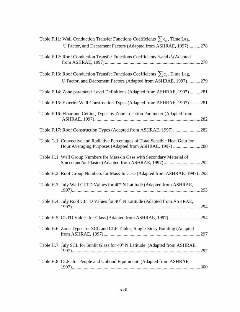
xxii
Table F.11: Wall Conduction Transfer Functions Coefficients nc , Time Lag,
U Factor, and Decrement Factors (Adapted from ASHRAE, 1997) .......... 278
Table F.12: Roof Conduction Transfer Functions Coefficients bnand dn(Adapted
from ASHRAE, 1997) ................................................................................. 278
Table F.13: Roof Conduction Transfer Functions Coefficients nc , Time Lag,
U Factor, and Decrement Factors (Adapted from ASHRAE, 1997) ........... 279
Table F.14: Zone parameter Level Definitions (Adapted from ASHRAE, 1997) ......... 281
Table F.15: Exterior Wall Construction Types (Adapted from ASHRAE, 1997) ......... 281
Table F.16: Floor and Ceiling Types by Zone Location Parameter (Adapted from
ASHRAE, 1997) .......................................................................................... 282
Table F.17: Roof Construction Types (Adapted from ASHRAE, 1997) ....................... 282
Table G.1: Convective and Radiative Percentages of Total Sensible Heat Gain for
Hour Averaging Purposes (Adapted from ASHRAE, 1997) ....................... 288
Table H.1: Wall Group Numbers for Mass-In Case with Secondary Material of
Stucco and/or Plaster (Adapted from ASHRAE, 1997) ............................... 292
Table H.2: Roof Group Numbers for Mass-In Case (Adapted from ASHRAE, 1997) . 293
Table H.3: July Wall CLTD Values for 40 N Latitude (Adapted from ASHRAE,
1997) ............................................................................................................. 293
Table H.4: July Roof CLTD Values for 40 N Latitude (Adapted from ASHRAE,
1997) ............................................................................................................. 294
Table H.5: CLTD Values for Glass (Adapted from ASHRAE, 1997) ........................... 294
Table H.6: Zone Types for SCL and CLF Tables, Single-Story Building (Adapted
from ASHRAE, 1997) .................................................................................. 297
Table H.7: July SCL for Sunlit Glass for 40 N Latitude (Adapted from ASHRAE,
1997) ............................................................................................................. 297
Table H.8: CLFs for People and Unhood Equipment (Adapted from ASHRAE,
1997) ............................................................................................................. 300
1
CHAPTER I
INTRODUCTION
1.1 Background
Today, buildings consume a large portion of the total United States energy use. A
recent study by Lawrence Livermore National Laboratory (LLNL, 2014) showed that the
total United States (U.S.) energy use in 2014 was approximately 98.3 Quads (1 Quad =
1015 Btu, QBtu). In the LLNL study, the three main energy end-use sectors included:
buildings (residential + commercial), industrial and transportation, which consumed
20.73 QBtu (28.6%), 24.7 QBtu (34.1%) and 27.1 QBtu (37.3%), respectively.
In the LLNL 2014 study, the buildings sector (i.e., residential + commercial)
accounted for 20.73 QBtu or about one third of the end-use energy use in the U.S. in
2014. However, if the energy waste from the electricity production is considered and the
waste from this sector is proportioned according to the end-use, the buildings sector was
responsible for 40.3 QBtu of total U.S. source energy consumption. Therefore, buildings
represent 41% of total U.S. source energy use. Clearly, designing more energy efficient
buildings will have a major impact on reducing future U.S. source energy use.
The building industry has responded to this need with efforts to improve commercial
building energy efficiency in the past 39 years since the 1973 oil embargo. The first
commercial building energy standard, ASHRAE Standard 90-1975, was published by
the American Society of Heating, Refrigerating and Air-Conditioning Engineers
(ASHRAE) as a direct response to the 1973 energy crisis (Skalko, 2012). Since then, a

2
series of new, more stringent energy codes were published, including: the 1977 Model
Energy Code (MEC), ASHRAE Standard 90A-1980, ASHRAE Standard 90B-1975, the
1983-1986 MEC, the 1988 MEC, ASHRAE Standard 90.1-1989, the 1992 MEC, the
1995 MEC, ASHRAE Standard 90.1-1999, the 2003 IECC, the 2004 IECC, ASHRAE
Standard 90.1-2004, the 2006 IECC, ASHRAE Standard 90.1-2007, the 2009 IECC,
ASHRAE Standard 90.1-2010 and the 2012 IECC. Presently, there are several published
standards and guidelines for building designs, including: the minimum standards for
energy efficiency – ASHRAE Standard 90.1-2013 (ASHRAE, 2013b) and the 2015
International Energy Conservation Code (ICC, 2015a); ASHRAE’s Advanced Energy
Design Guides (30% AEDG1 and 50% AEDG2); and high-performance green building
standards - ASHRAE Standard 189.1-2014 (ASHRAE, 2014) and the 2015 International
Green Construction Code - IGCC (ICC, 2015b).
As a result of increasing energy prices, environmental concerns and improved
building energy standards, there is an increasing effort to analyze, design and construct
new high performance buildings that will be affordable, consume less energy, look
appealing, and provide acceptable indoor air conditions. However, in many cities in the
U.S. developers are asked to try to reuse some portion of an existing structure, or add-on
to an existing structure without really knowing how that previous building was designed,
especially the HVAC system. Often, older buildings have existing HVAC systems that
are significantly over-sized, which makes them inefficient for meeting the heating and
1 The 30% AEDG include: small hospital and healthcare facilities (ASHRAE,2009a), highway lodging (ASHRAE, 2009b), small warehouses and self-storage buildings (ASHRAE, 2008a), K-12 school buildings (ASHRAE, 2008b), small retail buildings
(ASHRAE, 2008c), and small office buildings (ASHRAE, 2004). 2 The 50% AEDG include: large hospitals (ASHRAE, 2012), K-12 school buildings (ASHRAE, 2011b), small to medium office buildings (ASHRAE, 2011c), and medium to big box retail buildings (ASHRAE, 2011d).
3
cooling loads they must supply. In some cases, the thermal mass of these older buildings
has never been adequately taken into account during the design process, which may have
led to the significant over-sizing errors in the thermal load calculations. Furthermore,
efforts to develop net-zero buildings, for example, the Research Support Facility (RSF)
designed by National Renewable Energy Laboratory (NREL) are adding another layer of
efficiency requirements to building design. Finally, many characteristics are not easily
incorporated into the peak load design calculation, such as natural ventilation, underfloor
air distribution, radiant slabs, etc.
Currently, several peak load cooling calculation methods are in use, including: the
Total Equivalent Temperature Difference/ Time Averaging (TETD/TA) Method, the
Heat Balance Method (HBM), the Transfer Function Method (TFM), the Cooling Load
Temperature Difference/Solar Cooling Load/Cooling Load Factor (CLTD/SCL/CLF)
Method and the Radiant Time Series Method (RTSM). Since 2001, detailed descriptions
of the TFM, the TETD/TA Method and the CLTD/SCL/CLF Method have been
removed from ASHRAE Handbook of Fundamentals with only the HBM and the RTSM
remaining. At the 2016 ASHRAE winter conference, in one of the seminar presentations,
Professor Jeffrey Spitler provided an overview of how ASHRAE Technical Committee
TC 4.1 decided to replace the previous three simplified methods with only the RTSM
(Spitler, 2016). In this presentation, it was explained that TC 4.1 had received numerous
complaints from ASHRAE members about how confusing it was to have all three
methods included in one Handbook. As a result, TC 4.1 decided to replace the discussion
4
of the three methods with only one discussion about the RTSM and only brief
summaries about the other methods.
However, no clear comprehensive comparative studies have been found to clarify the
differences that arise when calculating the peak cooling load with all the different
methods. Therefore, whether the RTSM can actually replace all previous methods used
by architects and engineers, and perform a reasonable prediction of peak cooling loads
remains to be seen.
As of result of these issues, there is a need for a better understanding of how
effective the existing peak cooling load calculation methods are for commercial building
design in the U.S., including current methods in the ASHRAE Handbook compared with
the previously published methods, and how/whether those methods are being used
effectively by engineers.
1.2 Purpose and Objectives
The purpose of the current study is to analyze and compare building peak cooling
load calculation methods, and to determine how effectively those methods are being
used by architects and engineers. The long-term goal of this work is to improve the use
of peak cooling load predictions that are used by architects and engineers to size HVAC
systems in commercial buildings.
The following objectives were accomplished:
A literature review of the existing peak cooling load calculation methods for
commercial buildings in the U.S.,
5
A survey and interview of field professionals to determine what methods are
used today in the HVAC design,
The selection of a representative case-study building for comparing the peak
cooling load methods,
The application of the peak cooling load design methods to the case study
building,
A search to investigate the possible shortcomings of today’s peak cooling load
design methods,
The development of recommendations regarding peak cooling load design
methods.
1.3 Significance and Limitations of the Study
This study is significant because of the following:
It provides a thorough literature review on the history of peak cooling load
design methods;
It provides a comprehensive document of all peak cooling load methodologies
that were included in the ASHRAE Handbook of Fundamentals from 1967-2013;
It compares all peak cooling load design methods in use in the U.S., including:
the HBM; the RTSM; the TFM; the TETD/TA Method; and the CLTD/SCL/CLF
Method.
It proposes and documents new SCL table updates for the CLTD/SCL/CLF
Method based on the ASHRAE RTSM Spreadsheet Tool.
6
The current study has the following limitations:
The study focuses only on the building envelope peak cooling loads only, and
does not cover cooling loads coming from internal heat gains, HVAC system and
plant;
Only sensible peak cooling loads are studied, which does not cover the latent
cooling loads;
The pool of participants for the survey and interview was drawn from a limited
group of participants;
Peak cooling load methods not published in the ASHRAE Handbook of
Fundamentals were not analyzed or compared in this study.
1.4 Organization of the Dissertation
This dissertation is organized as follows:
In Chapter I, the study background is provided as well as the study purpose and
objectives, followed by the study significance and the limitations.
In Chapter II, a comprehensive literature review was performed, covering the history
of related science and the peak cooling load calculation methods. The first section tracks
the early science development that lead to dynamic heat transfer analysis methods,
including: gas laws, heat transfer and thermodynamics. The second section reviews the
history of the major peak heating and cooling load calculation methods in four different
periods: Pre-1945, 1946-1969, 1970-1989, and 1990-Present. It also summaries the five
existing peak cooling load design calculation methods, which are the Heat Balance
Method (HBM), the Total Equivalent Temperature Difference/Time Averaging Method
7
(TETD/TA), the Transfer Function Method (TFM), the Cooling Load Temperature
Difference/Solar Cooling Load/Cooling Load Factor Method (CLTD/SCL/CLF), and the
Radiant Time Series Method (RTSM). In the last section, previous comparisons related
to this work are reviewed.
In Chapter III, the research methodology is presented, including: the procedure used
to survey and interview field professionals; the comparison analysis procedure of the
peak cooling load design calculation methods; and a proposed improved peak cooling
load design methodology.
In Chapter IV, the study results are shown. In Part I, the survey and interview results
are shown. Part II provides the results of the base-case analysis comparison of the peak
cooling load design methods. Finally, additional case studies are presented for all
methods in Part III, followed by a summary of the findings.
In Chapter V, the proposed new SCL table updates for the CLTD/SCL/CLF Method
are developed.
Finally in Chapter VI, result summary and conclusions are provided from the study
and the potential future work is discussed.
8
CHAPTER II
LITERATURE REVIEW*
2.1 Overview
Currently, there is an increasing interest in the HVAC community to analyze, design
and construct new high performance buildings that will consume less energy, look
appealing, and provide acceptable indoor air conditions. However, in many cities in the
U.S. developers are asked to try to reuse some portion of an existing structure, or add-on
to an existing structure without really knowing how that previous building was designed,
especially the HVAC systems. Often, older buildings have existing HVAC systems that
are significantly over or under sized, which makes them inappropriate for meeting the
heating/cooling loads they must supply. In some cases, the thermal mass of these older
buildings has never been adequately taken into account during the HVAC design process,
which may have led to large errors in the thermal load sizing calculations that produces
inefficient, oversized systems.
Although there have been a number of previous papers that have presented historical
discussions of the origins of computer simulation programs, few if any studies have
provided an historical analysis of peak heating and cooling load calculation methods that
covered periods before computerized simulations came into use (Feldman and Merrian,
1979; Kusuda, 1985; Stamper,1995; Sowell and Hittle, 1995; Shavit, 1995).
*Part of this chapter is reprinted from Peak Heating/Cooling Load Design Methods: How We Got to Where We Are Today. Mao, C.,
Haberl, J.S. and Baltazar, J.C., 2013, Proceedings of BS2013: 13th Conference of International Building Performance Simulation Association, Chambéry, France, August 26-28. Copyright 2013 by original authors.

9
2.2 History of Science Related to Peak Load Calculation
The development of peak heating and cooling load calculations, and annual building
energy use calculation methods could not have been performed without a solid
foundation based on the related sciences. Therefore, a brief review of the previous
sciences and engineering practices from the 1700s to the 1900s is provided, including3:
gas laws, heat transfer, and thermodynamics.
2.2.1 Gas Laws
The development of the science of the behavior of gasses, such as moist air, was
important for sizing building heating and cooling systems. The earliest studies of gas
laws began in the 17th century first with experiments that defined temperature, pressure
and volume relationships, followed shortly thereafter with a better understanding of
partial gas pressures, molecules and eventually atoms. One of the earliest studies was
performed by the British scientist and philosopher, Robert Boyle (1627-1691), who
performed experiments with an air vacuum pump to observe the effects of reducing air
pressure, which was reported in his book “New Experiments Physico-Mechanicall,
Touching the Spring of the Air, and its Effects” in 1660 (West, 2005; Donaldson et al.,
1994); Two years later, he published his results, which demonstrated that the product of
gas pressure and volume was constant at a given temperature; now referred to as
“Boyle's Law”. Robert Boyle is usually credited with being the first to research gas
properties through observations based on experiments (Donaldson et al., 1994).
3 Adapted from Mao et al. (2012, 2013).
10
One hundred years later, in 1787, Jacques Charles (1746-1823), the French chemist
and physicist, formulated Charles' Law (Acott, 1999; Donaldson et al., 1994), which
stated that the gas volume was proportional to the gas temperature at a given gas
pressure. However, Charles' Law was not published until 1802 when it was cited by
Joseph Louis Gay-Lussac (Elena and Manuela, 2006), a French chemist and physicist.
Gay-Lussac's Law showed the relationship between gas pressure and temperature at a
constant gas volume. A combined gas law that considered gas pressure, temperature and
volume was later derived by combining Boyle's Law and Charles' Law (Sandfort, 1962;
cited in Donaldson et al., 1994).
In 1801, the English chemist, meteorologist and physicist, John Dalton (1766-1844),
introduced the concept of “partial pressure” (Woo and Yeo, 1995; Donaldson et al.,
1994), which proposed that the summation of the partial pressures of each gas
component was equal to the total pressure of mixture. This later became known as
"Dalton's Law". Eight years later, in 1809, Joseph Louis Gay-Lussac developed another
law about the conservation of gas volumes in chemical reactions at the same temperature
and pressure (Elena and Manuela, 2006). In 1811, based on Gay-Lussac's data, Amedeo
Avogadro (1776-1856) proposed Avogadro's Law, which was the first to suggest that
"molecules" should be differentiated from “atoms” (Elena and Manuela, 2006), which
helped to further understand gaseous mixture. Avogadro's Law also stated that gases
with equal volumes at the same temperature and pressure had equal numbers of
molecules (Hirang, 2008-2009). Eventually, all these discoveries lead to the Ideal Gas
Law that formed the basis of today’s thermodynamic principles for moist air.

11
2.2.2 Heat Transfer
Heat transfer, the discipline that studies the process of transferring heat from one
object to another, is composed of three important fields: conduction, convection and
radiation. The earliest theories of heat transfer began with Isaac Newton (1642-1727)
who published “Newton's Law of Cooling” in 1701 that first introduced the term “heat
transfer coefficient” (Bergles, 1988). Newton proposed a proportional relationship
between the cooling rate and the temperature difference of two surfaces based on his
early experiments. His Law of Cooling was considered the beginning of convective heat
transfer studies. The three modes of heat transfer: conduction, convection and radiation,
were not separately distinguished until 1757 by Joseph Black (1728-1799), who also
introduced the term "Latent Heat" (Cheng and Fujii, 1988).
In 1807, the theory of heat conduction was first formulated by Joseph Fourier (1768-
1830) through the use of partial differential equations that described the transient process
(Narasimhan, 1999). Fifteen years later, in 1822, Fourier's Law of Heat Conduction was
formally proposed in his published paper “The Analytic Theory of Heat” (Donaldson et
al., 1994). In the beginning of the 19th century, the earliest work on radiation heat
transfer started with the recognition of “invisible light” by William Herschel in 1800
(Backman and Harman, 2011; Donaldson et al., 1994). It was not until sixty years later,
in 1860, that Kirchhoff’s law of radiation was formulated by Gustav Kirchhoff (l824-
1887) (Mätzler, 2012), which gave us an equation to calculate the radiative heat transfer
process at the surface of a material. Shortly after this, Stefan's Law was proposed in
1879, based on experiments performed by Joseph Stefan (1835-1893), which stated that

12
there was a proportional relation between radiation and the fourth power of surface
temperature. Then, five years later, in 1884, Ludwig Boltzmann (1844-1906) provided a
derivation of a fourth power radiative heat transfer law (Carter, 2004). Stefan and
Boltzmann’s work were later combined and are now referred to as the "Stefan-
Boltzmann Law", which includes the Stefan-Boltzmann constant for performing the
radiative heat transfer calculation. In summary, these heat transfer discoveries provided
the basic theories and equations that were needed to calculate dynamic building peak
load calculations as well as annual energy use calculations.
2.2.3 Thermodynamics
Thermodynamics is a discipline that combines the concepts of heat, work and
energy, including: the First, Second and Third Law of Thermodynamics. The science of
thermodynamics developed gradually alongside the development of gas laws and heat
transfer in the 19th century (Cheng and Fujii, 1988). Beginning in 1824, Sadi Carnot
(1796-1832), also known as the "Father of Thermodynamics", proposed the Carnot
cycle, which was published in his “Reflections on the Motive Power of Fire and on
Machines Filled to Develop That Power” (Donaldson et al., 1994); this paper marked the
birth of the science of thermodynamics and established the foundation for the First and
Second Law of Thermodynamics. The First Law of Thermodynamics – the Conservation
of Energy was first introduced in 1842 by Robert Mayer (1814-1878) who proposed that
heat was a form of energy (Cheng and Fujii, 1988; Donaldson et al., 1994). One year
13
later, the equivalence of heat and mechanical work was demonstrated by James Prescott
Joule (1818-1889)4 (Donaldson et al., 1994).
In 1847, an energy conservation formula was first proposed by Hermann von
Helmholtz (1821-1894) (Donaldson et al., 1994). This led to the development of the
Second Law of Thermodynamics, which was presented by Rudolf J. Clausius (1822-
1888) in 1850 when be introduced the term "entropy", which was based on Helmholtz
and Carnot's work (Powers, 2012; Donaldson et al., 1994). The Third Law of
Thermodynamics was not proposed until 1906 by the physical chemist, Walther
Hermann Nernst (1864-1941), which stated that the entropy of a system was zero if the
temperature was absolute zero (Javadi, n.d.). These three Laws of Thermodynamics
helped consolidate the concepts of heat, work and energy into calculations of a single
subject or system of equations, which together with the science of gas laws and heat
transfer became the foundations of building peak heating and cooling load calculations
and annual energy use calculations.
2.3 Peak Load Calculation Methods
Building peak load calculation methods, which include peak heating and cooling
load calculations, are used for sizing HVAC equipment in order to provide adequate
heating or cooling when extreme weather conditions occur. This section reviews the
history of the major peak heating and cooling load methods in four different periods: Pre
1945, 1946-1969, 1970-1989, and 1990-Present.
4 The S.I. energy unit was named after James Prescott Joule.

14
2.3.1 Pre 1945
The birth of most engineering methods is often inspired by the need to solve
problems that were relevant and practical for a given period. Prior the development of
standardized peak load calculation methods, most engineers tried to design building
HVAC systems by relying on manufacturer’s literature for a specific system, a few
available textbooks, even fewer handbooks or guidebooks.
The earliest heating and ventilating design developments started in the nineteenth
century. Unfortunately, engineers had to design systems with rules-of-thumb or
approximate design methods because useful textbooks or guidebooks that were based on
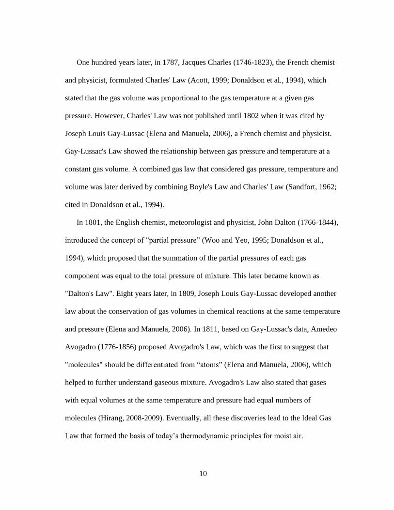
first principles were in scarce supply. As early as in 1834, Dr. Boswell Reid redesigned
the heating and ventilating system for British House of Commons using a chimney to
induce air flow through the building5, as shown in Figure 2.1, with a water spray cooling
and steam heating system (Donaldson et al., 1994). This was probably one of the first
successful applications of purposeful “fresh air” into a public space, with evaporative
cooling and/or heating applied to the air under manual controls.
5 This is because reliable air-handling units were not available.
15
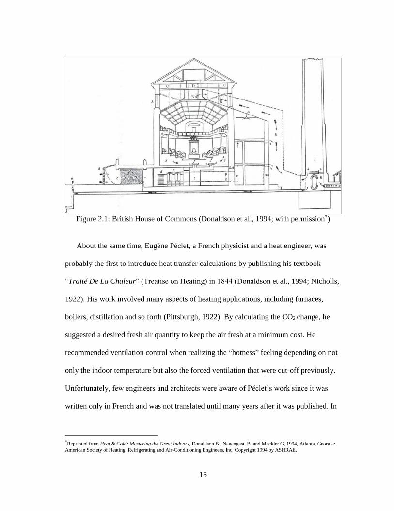
Figure 2.1: British House of Commons (Donaldson et al., 1994; with permission*)
About the same time, Eugéne Péclet, a French physicist and a heat engineer, was
probably the first to introduce heat transfer calculations by publishing his textbook
“Traité De La Chaleur” (Treatise on Heating) in 1844 (Donaldson et al., 1994; Nicholls,
1922). His work involved many aspects of heating applications, including furnaces,
boilers, distillation and so forth (Pittsburgh, 1922). By calculating the CO2 change, he
suggested a desired fresh air quantity to keep the air fresh at a minimum cost. He
recommended ventilation control when realizing the “hotness” feeling depending on not
only the indoor temperature but also the forced ventilation that were cut-off previously.
Unfortunately, few engineers and architects were aware of Péclet’s work since it was
written only in French and was not translated until many years after it was published. In
*Reprinted from Heat & Cold: Mastering the Great Indoors, Donaldson B., Nagengast, B. and Meckler G, 1994, Atlanta, Georgia:
American Society of Heating, Refrigerating and Air-Conditioning Engineers, Inc. Copyright 1994 by ASHRAE.
16
1904, some of Péclet’s work was finally translated into English by Charles Paulding
(Paulding, 1904).
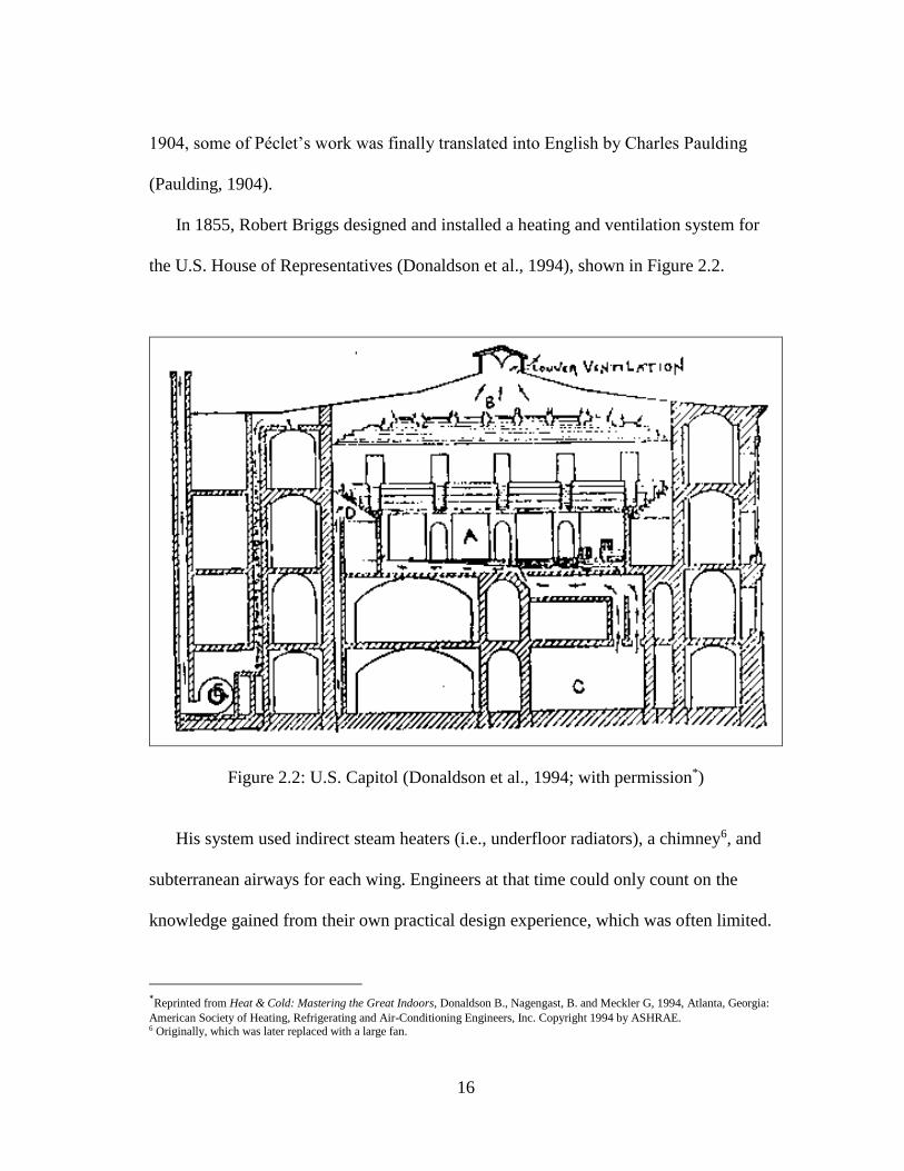
In 1855, Robert Briggs designed and installed a heating and ventilation system for
the U.S. House of Representatives (Donaldson et al., 1994), shown in Figure 2.2.
Figure 2.2: U.S. Capitol (Donaldson et al., 1994; with permission*)
His system used indirect steam heaters (i.e., underfloor radiators), a chimney6, and
subterranean airways for each wing. Engineers at that time could only count on the
knowledge gained from their own practical design experience, which was often limited.
*Reprinted from Heat & Cold: Mastering the Great Indoors, Donaldson B., Nagengast, B. and Meckler G, 1994, Atlanta, Georgia:
American Society of Heating, Refrigerating and Air-Conditioning Engineers, Inc. Copyright 1994 by ASHRAE. 6 Originally, which was later replaced with a large fan.
17
In the U.S., useful textbooks that contained design tables and equations did not start to
appear until twenty to thirty years later.
In 1884, Frank E. Kidder introduced the first version of his book “Architect’s and
Builder’s Handbook” (Kidder, 1906). This book was oriented towards architects and
mostly contained information from manufacturer’s literature regarding the sizing of
steam radiators by the determination of the room size and boiler size. Although a heat
loss calculation method was included, it was described using words instead of equations.
In addition, thermal mass was not considered in the HVAC system design, since all
tabulated heat transfer coefficients were for steady-state calculations.
Shortly after, in 1894, a professor of the Technical University of Berlin, Hermann
Rietschel published a German textbook called “Lüftungs-und Heizungs-Anlagen”7
(Ventilation and Heating Systems) that was later translated into English version by C.W.
Brabbee in 1927 (Rietschel and Brabbee, 1927). This book is widely recognized as
Europe’s first scientifically-based text on heating and ventilating. It contained relatively
complete information about how to calculate heat transfer, including equations that are
still in use today. It also described how to size steam systems, piping, etc., and it even
provided a detailed solution to the dynamic heat transfer calculation in a single slab of
wall material as well as steady-state heat loss calculations for walls, roofs, windows and
ventilation. The book also included tables of useful heat transfer coefficients as well as
charts and graphs with plotted properties of moist air (Usemann, 1995). Unfortunately,
no formulas for moist air were included.
7 Private communication with Mr. Bernard Nagengast.
18
Shortly after, in 1896, Rolla Carpenter, a professor at Cornell University, published
the first version of his textbook named Heating and Ventilating Buildings (Carpenter,
1896). This book included theory and applications of heating and ventilating apparatus
by Thomas Tredgold (1836), Charles Hood (1855), and Eugéne Péclet (1850). It also
included tables of materials, properties of air and math equations, which makes it
equivalent to one of today’s engineering handbook.
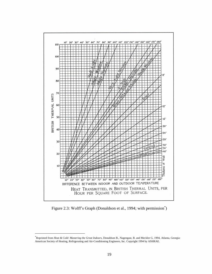
Around the same period, in the 1890s, Alfred R. Wolff, a well-known heating and
ventilating design engineer in the U.S., published his “heat transfer coefficient” chart
that was derived from the previous work by Eugéne Péclet and Thomas Box. It included
a graph that showed the heat loss per unit area for windows, doors and walls and ceilings
of varying thickness (Wolff, 1894; cited in Donaldson et al., 1994). Wolff was regarded
as one of the first U.S. engineers to use “heat transfer coefficients”, and his chart that
showed “varying thickness” was probably the first published graph that estimated the
dynamic effect of thermal mass, shown in Figure 2.3. Wolff was the best known as the
designer of the air-conditioning system8 for the Board Room of the New York Stock
Exchange9 in 1903, which is regarded as one of the earliest commercial air-conditioning
systems to be designed and operated for comfort in the U.S. (Donaldson et al., 1994).
8 Alfred Wolff consulted Henry Torrance of the Carbondale Machine Company for this design (Donaldson et al., 1994). 9 Two years later, in 1905, Stuart Cramer first used the term “air conditioning” for treating air in textile mills in N.C., which became widely adapted as the terminology that described artificial cooling system (Donaldson et al., 1994).
19
Figure 2.3: Wolff’s Graph (Donaldson et al., 1994; with permission*)
*Reprinted from Heat & Cold: Mastering the Great Indoors, Donaldson B., Nagengast, B. and Meckler G, 1994, Atlanta, Georgia:
American Society of Heating, Refrigerating and Air-Conditioning Engineers, Inc. Copyright 1994 by ASHRAE.
20
Stepping into the 20th century, new peak cooling load methods began to be
developed during the 1900 to 1945 period, including: the psychrometric chart and the
governing equations for moist air (Carrier, 1911), the sol-air temperature method
(Mackey and Wright, 1944) and the thermal network method (Paschkis, 1942). In 1902,
a young engineer at the Buffalo Forge company, named Willis Carrier designed his first
ventilation system with cooling coils for the Sackett and Wilhelms Company, in
Brooklyn, N.Y. (Donaldson et al., 1994). Unfortunately, the system was not successful,
because, although it could cool the air stream, it could not control the humidity inside the
building. After studying the failure, Carrier determined that a spray-type air washer
using chilled water could be used to control temperature and humidity10.
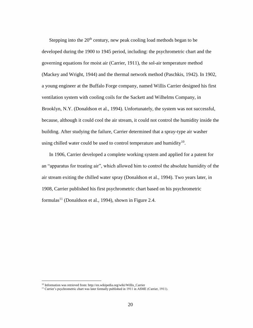
In 1906, Carrier developed a complete working system and applied for a patent for
an “apparatus for treating air”, which allowed him to control the absolute humidity of the
air stream exiting the chilled water spray (Donaldson et al., 1994). Two years later, in
1908, Carrier published his first psychrometric chart based on his psychrometric
formulas11 (Donaldson et al., 1994), shown in Figure 2.4.
10 Information was retrieved from: http://en.wikipedia.org/wiki/Willis_Carrier 11 Carrier’s psychrometric chart was later formally published in 1911 in ASME (Carrier, 1911).

21
Figure 2.4: First Psychrometric Chart (Carrier, 1911; with permission*)
In 1928, Carrier designed the mechanical system for the Milam Building in San
Antonio, Texas, which was the first high-rise, air-conditioned office building in U.S.
(ASME, 1991), shown in Figure 2.5. In the Milam building two centrifugal refrigeration
units, developed by the Carrier Company, were used as the cooling system.
Unfortunately, the radiant heat that was supposed to be absorbed by the heavy exterior
construction was not well understood. This resulted in the HVAC system not working as
planned due to an unexpected asymmetric East-West cooling load. To remedy this,
* Reprinted from Rational Psychrometric Formulae, Carrier, W.H., 1911, ASME Transactions, 33, 1005-
1053. Copyright 1911 by ASME.
22
venetian blinds, cloth window shades and duct dampers were installed and manually
operated to solve morning or afternoon overheating problems (ASME, 1991).
In 1914, the Buffalo Forge Engineer’s Handbook was published, which was
recognized as the first comprehensive U.S. manufacturer’s handbook for heating and
ventilating (Carrier, 1914). It contained detailed equations for heat loss calculations for
walls, roofs, windows and ventilation, including tables of useful coefficients as well as
Carrier’s psychrometric chart, which was the first time that a psychrometric chart was
introduced in a handbook. Eight years later, in 1922, ASHVE published its first guide
book, “The American Society of Heating and Ventilating Engineers Guide”, which also
had basic heat loss formula, unfortunately which were presented as “word formulas”
(ASHVE, 1922).
During this period, several other useful textbooks appeared. In 1918, John R. Allen
et al. published the first edition of their book “Heating and Ventilation” that provided
detailed heat loss calculation methods that also included tables of useful coefficients and
equations (Allen et al., 1931).
Shortly after Allen et al.’s book was published, Charles Merrick Gay together with
Charles De Van Fawcett published their first textbook in 1935, which contained detailed
equation-based calculations for heat loss and a very terse advice about how to calculate
summertime heat gain12 (Gay and Fawcett, 1937). One year later, the TRANE Company
published its first design manual, which provided a load estimate sheet for engineers to
12 In the book, they recommended the use of a rule-of-thumb method: “add 25°F to the dry bulb temperature difference for heat transmission calculation”.

23
use (TRANE, 1938). This design manual used tabulated “solar temperature differences”
and also included instructions for using the TRANE air - conditioning slide ruler13.
Figure 2.5: The Milam Building (ASME, 1991; with permission*)
13 This slide ruler was for use with the TRANE psychrometric chart. Interestingly, the TRANE heat transfer tables were listed
according to the color of the wall, versus thermal mass characteristics. *Reprinted from The Milam Building, San Antonio, Texas: A National Mechanical
Engineering Heritage Site. New York: ASME Book No. HH9106. Copyright 1991 by National Mechanical Engineering Heritage.

24
Several important papers were also published during this period in Europe and in the
U.S. In 1925 in Europe, the Response Factor Method was first introduced for transient
flow calculation by André Nessi and Léon Nisolle in France (Nessi and Nisolle, 1925).
In 1939 in the U.S., Alford et al. published a paper on the heat storage/heat transfer
through walls driven by temperature and solar intensity in the ASHVE Transactions.
Their paper provided a detailed solution to the differential equation in the form of a
decrement factor and a time delay (Alford et al., 1939). Three years later, in 1942, the
thermal R/C network method was first published by Victor Paschkis to calculate the
dynamic heat transfer through building walls (Paschkis, 1942). Later in 1944, C.O.
Mackey and L.T. Wright Jr. used a modified version of Alford et al.’s equations and
proposed the “sol-air temperature method” (Mackey and Wright, 1944). Using the sol-air
temperature method, the inside surface temperature of building material can be
calculated using a daily average sol-air temperature, a constant indoor temperature, a
decrement factor and a time lag for homogeneous walls shown in Figure 2.6. In the same
year, in 1944, John G. Linvill and John J. Hess Jr. published their article “Studying
Thermal Behavior of Houses”, which was an undergraduate student project at M.I.T.
Their article showed how the thermal R/C network method could be used to simulate the
dynamic heat transfer of an entire house (Linvill and Hess, 1944).

25
Figure 2.6: Decrement Factor Graph (Mackey and Wright, 1944; with permission*)
In summary, during the period prior to 1945, there were at best inconsistent methods
for calculating peak heating and cooling loads. Some methods contained the seeds of the
dynamic heat transfer calculations used today, others were rough estimation. These
methods appeared in textbooks, handbooks, guidebooks and manufacturer’s literature
published during this period. However, during this same period, the foundation was laid
for today’s modern methods, which began with sol-air temperatures, decrement factors
and the use of a thermal R/C network to calculate dynamic building heat gain/loss.
2.3.2 1946-1969
Most of the manual peak cooling calculation methods used today in the U.S. were
proposed during the 1946-1969 period. In 1948, as a design engineer at Carrier
* Reprinted from Periodic Heat Flow – Homogeneous Walls or Roofs, Mackey, C.O. and Wright, L.T., Jr. 1944, ASHVE Journal,
16(9), 546-555. Copyright 1944 by ASHRAE.
26
Corporation, James P. Stewart was the first to outline Equivalent Temperature
Differentials (ETD), which were based on Mackey and Wright’s earlier work (Stewart,
1948), that was intended to be an easy-to-use tabulated design method that would
estimate the dynamic heat gains through the walls and roofs. Stewart’s ETD tables were
generated under specific conditions: 1) July at 40 N Latitude; 2) maximum and
minimum outdoor temperatures of 95 F and 75 F; and 3) a room temperature of 80 F.
If the temperature difference between the outdoor maximum design temperature and the
room temperature were larger (or smaller) than 15 F, it was suggested to use the
published ETD and add (or subtract) the difference (Stewart, 1948). The ETD tables
were adopted for use in the 1951 ASHVE Guide and 1961 ASHRAE Guide and Data
Book (ASHVE, 1951; ASHRAE, 1961). Total Equivalent Temperature Difference/ Time
Averaging Method (TETD/TA) were later tabulated in the 1967 ASHRAE Handbook of
Fundamentals (ASHRAE, 1967) by adding the Time Averaging (TA) Procedure and
suggesting that the method was suitable for calculating extended hourly profiles only if
the radiant heat gain components were averaged over the representative period for all the
thermal mass of the building. Unfortunately, judging the amount of thermal mass in a
building was a difficult job for an average engineer, which ultimately made the method
useful only in the hands of an experienced engineer. Appendix G details the TETD/TA
Method calculations.
In 1955, a new edition of Gay and Fawcett’s textbook was published that included a
new author, William McGuinness who was a professor of Architecture at the Pratt
Institute of Technology (Gay et al., 1955). This new edition included a revised procedure
27
for air-conditioning design, as well as improved data for calculating heat gains, which
referenced the ETD tables in the 1951 ASHVE Guide14. So, by the mid-1950s either the
direct use of Mackey and Wright’s sol-air temperature equations or the TETD/TA
Method provided designers with an improved manual method to calculate the impact of
thermal mass on the dynamic heat gain.
In the mid-1950, W.R. Brisken, S.G. Reque and P.R. Hill laid the foundations of
today’s thermal Response Factor Method (RFM), based on Nessi and Nisolle’s 1925
work. In 1956, Brisken and Reque published their heat load calculations using the RFM
(Brisken and Reque, 1956). In this method, they proposed using “square waves” to
represent a time-varying “curve” of dynamic temperature response. One year later, Hill
developed a more accurate “unit triangle” method for calculating the time-varying 1-D
surface temperature (Hill, 1957). Based on these works, in 1967, Gintas Mitalas and Don
Stephenson developed the thermal Response Factor Method (RFM), which allowed for
the solution to the dynamic heat transfer problem without having the knowledge of how
to solve a separate differential equation for each new wall type (Mitalas and Stephenson,
1967; Stephenson and Mitalas, 1967). Later, this method became part of the Transfer
Function Method that is also called the Weighting Factor Method (Mitalas, 1972;
ASHRAE, 1981).
Beginning in the 1940s, several authors investigated the use of thermal R/C network
models for analyzing dynamic heat transfer (Paschkis, 1942; Buchberg, 1955; Nottage
and Parmelee, 1954). As previously mentioned, although the first thermal R/C network
14 Gay et al.’s book cited the 1951 ASHVE Guide as the source of the ETD tables, which were based on Mackey and Wright’s 1944 sol-air equation.
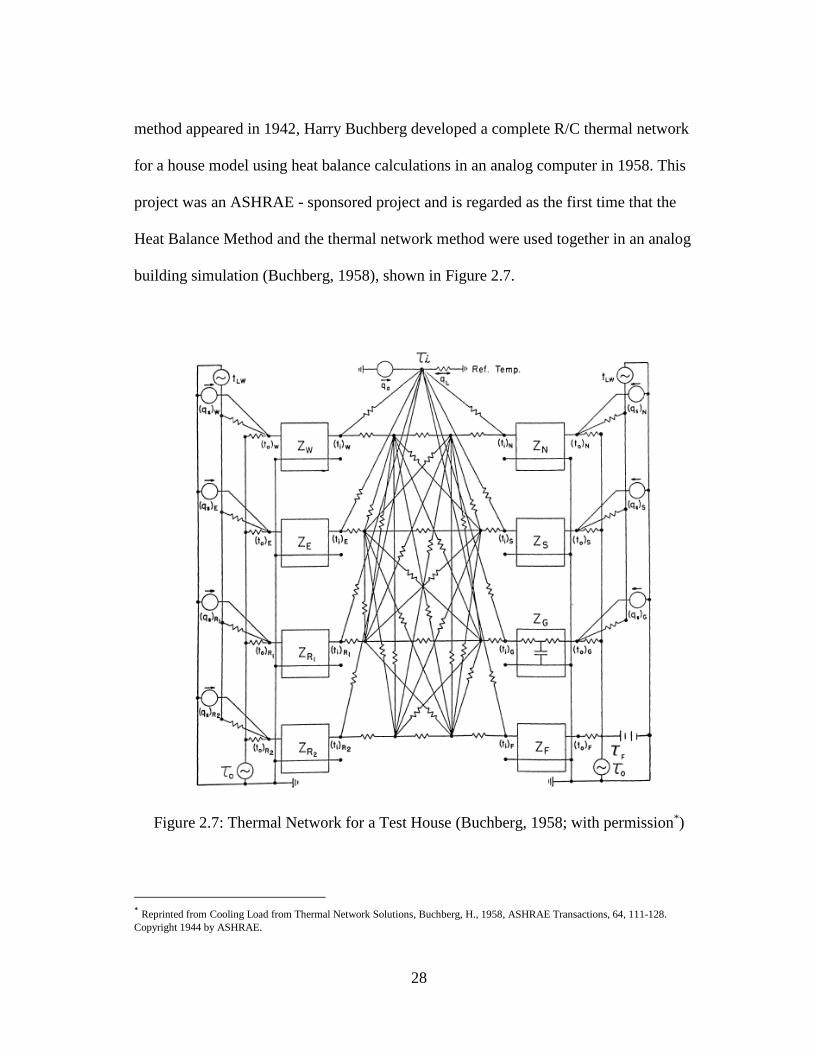
28
method appeared in 1942, Harry Buchberg developed a complete R/C thermal network
for a house model using heat balance calculations in an analog computer in 1958. This
project was an ASHRAE - sponsored project and is regarded as the first time that the
Heat Balance Method and the thermal network method were used together in an analog
building simulation (Buchberg, 1958), shown in Figure 2.7.
Figure 2.7: Thermal Network for a Test House (Buchberg, 1958; with permission*)
* Reprinted from Cooling Load from Thermal Network Solutions, Buchberg, H., 1958, ASHRAE Transactions, 64, 111-128.
Copyright 1944 by ASHRAE.
29
The Heat Balance Method was later included in the 1981 ASHRAE Handbook along
with the Weighting Factor Method (WFM) as building annual energy use calculation
methods (ASHRAE, 1981).
The guide books during the 1946 to 1969 period included: the 1951 ASHVE Guide
(ASHVE, 1951), the 1955 TRANE Air Conditioning Manual (TRANE, 1955), the 1960
Carrier Handbook of Air Conditioning System Design (Carrier, 1960), several ASHRAE
Guide and Data Book (ASHRAE, 1961, 1963, 1965), and the first version of ASHRAE
Handbook (ASHRAE, 1967). In these handbooks, thermal mass was considered either
using sol-air temperature calculations or the TETD/TA Method.
Besides the methods discussed above, two other widely used methods were
developed about this time to solve the time-varying heat transfer problems: the Finite
Difference/Finite Element Method (FDM/FEM) and the admittance method. The
FDM/FEM was introduced in 1960 (Clough, 1960; Forsythe and Wasow, 1960) in the
form of equations that could be directly used in computer algorithms. The admittance
method was originally developed in the U.K. by A.G. Loudon in 1968 (Loudon, 1968).
The concept of “Thermal Admittance” was first introduced in the U.K. in the Institution
of Heating and Ventilating Engineers Guide (IHVE) in 1970 (Goulart, 2004) to measure
the ability of building components to smooth-out the temperature swings within a 24-
hour cycle. This method was later adopted by the Charted Institution of Building
Services Engineers (CIBSE) and is now widely used in the U.K.
During 1946-1969 period, the first edition of ASHRAE Handbook appeared, which
adopted the available peak heating and cooling load methods from important published

30
papers. In addition, during this period, several of the popular textbooks and
manufacturer’s literature were updated to reflect the new methods as well. In summary,
steady-state peak heating calculation methods matured and time-varying cooling load
calculation methods that considered ambient temperature and solar radiation became
available for designers to use.
2.3.3 1970-1989
Peak cooling load methods continued to develop during the period 1970-1989. In
1972, the ASHRAE Task Group on Energy Requirements (TGER) first introduced the
Transfer Function Method (TFM) for peak cooling load calculation, which was based on
Mitalas and Stephenson’s earlier work (ASHRAE, 1972) and is considered the first,
wide-spread, computer-oriented method for solving dynamic heat transfer problems in
buildings in the U.S. (Mitalas, 1972). It utilized Conduction Transfer Function
coefficients and sol-air temperatures to calculate the dynamic conduction heat gains
from walls and roofs. By applying weighting factors, heat gains from all surfaces could
then be converted into the room cooling load. Appendix F introduces the detailed
calculation procedure of TFM.
However, even as new computer-based methods were being developed, manual,
tabulated methods continued to be updated and used because many engineers could not
justify the time and expense required by the computer methods. One such method, based
on the principles of TFM, is the Cooling Load Temperature Difference/Cooling Load
Factor Method (CLTD/CLF), which was developed by William Rudoy and Fernando
31
Duran in 1974 at University of Pittsburgh (Rudoy and Duran, 1974). It included
tabulated results of controlled-variable tests summarized in ASHRAE research project
RP-138 for cooling load calculations. The CLTD/CLF Method attempted to simplify the
two-step TFM and TETD/TA Method into a single-step technique, which was later
published in the 1977 ASHRAE Handbook of Fundamentals (ASHRAE, 1977). Eleven
years later, in 1988, the CLTD/CLF Method was modified by Prof. Edward Sowell at
California State University who ran 200,640 simulations to provide new tabulated values
(Sowell, 1988). That same year, Steven Harries and Faye McQuiston proposed
additional Conduction Transfer Function (CTF) coefficients to cover more roof and wall
construction groups in ASHRAE research project RP-472 at Oklahoma State University
(Harries and McQuiston, 1988).
In summary, during the 1970 to 1989 period, peak heating load calculation methods
remain unchanged while major advances were made in peak cooling load calculation
methods, which are still taught in today’s textbooks, but no longer exist in the current
2013 ASHRAE Handbook of Fundamentals (ASHRAE, 2013a)15.
2.3.4 1990-Present
In 1993, Jeffery Spitler et al. at Oklahoma State University updated the CLTD/CLF
Method to become the CLTD/SCL/CLF Method by introducing the term “Solar Cooling
Load (SCL)” for an improved solar heat gain calculation through fenestration (Spitler et
al., 1993). Using Spitler et al.’s method, tables of CLTD, SCL and CLF were generated
15 For non-residential buildings, the Heat Balance Method and Radiant Time Series Method are included in Chapter 18 for peak cooling load calculations methods in the 2013 ASHRAE Handbook of Fundamentals.
32
based on the TFM. Once the cooling load was obtained by the TFM, the values of
CLTD, SCL, and CLF could then be calculated by dividing the surface area and overall
U-factor for the tabulated wall and roof combination groups. This new CLTD/SCL/CLF
Method was later incorporated into the 1993 ASHRAE Handbook of Fundamentals
(ASHRAE, 1993). Appendix H details the cooling load calculation procedure for this
method.
The most current cooling load calculation method is the Radiant Time Series Method
(RTSM) that Spitler et al. developed in 1997, which is an improvement over all previous
methods (Spitler el al., 1997). In response to research proposed by ASHRAE Technical
Committee TC 4.1, the RTSM was derived directly from, but is simpler than, the Heat
Balance Method. In the RTSM, the 1-D time-varying conduction is calculated using 24-
term response factors. The RTSM converts the radiant portion of hourly heat gain to
hourly cooling loads using radiant time factors. The accuracy of the RTSM is similar to
that of the TFM if custom weighting factors and custom conduction transfer functions
were used for all components in a building.
In 1997, Curtis Pedersen et al. at the University of Illinois further developed the
HBM using a model with twelve surfaces. Their published work included a complete
description of the mathematical calculations for the heat balance process. (Pedersen et
al., 1997). Finally, in 2001, the ASHRAE building load calculation toolkit (LOADS
Toolkits) was developed by Professor Pedersen (Pedersen, et al., 2001), which provided
FORTRAN source codes for the heat balance calculations. The HBM procedure is
explained in detail in Appendix D.
33
For residential load calculations, the Residential Heat Balance (RHB) and the
Residential Load Factor (RLF) methods were developed by Charles Barnaby in 2004
(Barnaby et al., 2004). In a similar fashion as the RTSM and LOADS Toolkit, the RHB
method was developed to be a computer algorithm, which was also coded using
FORTRAN, while the RLF method was developed to be a simplified method that could
be used manually or with a spreadsheet.
In 2000, an extensive analysis was developed that compared peak cooling load
calculation methods in the U.S. and the U.K. by Simon Rees at Oklahoma State
University (Rees et al., 2000). This analysis concluded that the cooling load calculation
methods in the U.S. and U.K. have the possibility of converging in the future.
In 2006, a spreadsheet tool was proposed by TC 4.1 volunteers to generate the
custom CLTD and CLF tables using the RTSM16 (Bruning, 2016). In this spreadsheet,
for the window cooling load calculation, a window CLF table was used to combine the
cooling load from both conduction and solar heat gains, which eliminated the SCL
tables. However, this tool was never published by ASHRAE.
Finally in 2007, the RTSM was improved by Nigusse at Oklahoma State University
(Nigusse, 2007; Nigusse and Spitler, 2010). The original RTSM uses Periodic Response
Factors (PRFs) to calculate heat gains through opaque surfaces, while the improved
RTSM introduced Conduction Time Series Factors (CTSFs), which are a set of
dimensionless factors, to perform the calculations. In the improved method, the window
solar heat gains are determined by a solar heat gain coefficient (SHGC) instead of the
16 Personal communication with Mr. Steve Bruning in January 2016.

34
original shading coefficient (SC). Appendix E distinguishes the two versions of RTSM
and details the cooling load calculation procedure.
2.4 Peak Cooling Load Calculation Method Comparisons
Only a few studies have shown comparisons among the five most common methods
used in U.S. for calculating peak design cooling load. This section reviews the previous
studies that are related to peak cooling load design methods.
2.4.1 Comparisons among the TFM, the TETD/TA Method, and the CLTD/SCL/CLF
Method
Among all the ASHRAE Handbook of Fundamentals, only the 1993 and 1997
versions covered the total sensible cooling load comparisons of the TFM, the TETD/TA
Method, and the CLTD/SCL/CLF Method using the same one-story office building
example, located at 40 N latitude, shown in Figure 2.8 and Figure 2.9.

35
Figure 2.8: ASHRAE Example Office Building (ASHRAE, 1993; ASHRAE, 1997; with
permission*)
In the previous comparison, the TFM and the TETD/TA Methods had similar
dynamic cooling load profiles with the same peak time (at 4 P.M.) but they had different
peak cooling load values. The TETD/TA over-predicted by 13% when compared to the
TFM. Whereas, the CLTD/SCL/CLF Method presented a slightly different profile
pattern in the middle of the TETD/TA and the TFM, but over-predicted by 19.8% when
compared to the TFM.
However, errors found in the calculated sol-air temperatures for the TFM in the 1997
ASHRAE Handbook of Fundamentals were reported by Al-Rabghi and Al-Johani (Al-
*Reprinted from ASHRAE Handbook of Fundamentals, 1993, Atlanta, GA: American Society of Heating, Refrigerating and Air-
Conditioning Engineers, Inc. Copyright 1993 by ASHRAE.
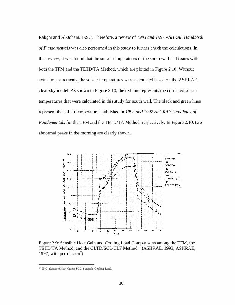
36
Rabghi and Al-Johani, 1997). Therefore, a review of 1993 and 1997 ASHRAE Handbook
of Fundamentals was also performed in this study to further check the calculations. In
this review, it was found that the sol-air temperatures of the south wall had issues with
both the TFM and the TETD/TA Method, which are plotted in Figure 2.10. Without
actual measurements, the sol-air temperatures were calculated based on the ASHRAE
clear-sky model. As shown in Figure 2.10, the red line represents the corrected sol-air
temperatures that were calculated in this study for south wall. The black and green lines
represent the sol-air temperatures published in 1993 and 1997 ASHRAE Handbook of
Fundamentals for the TFM and the TETD/TA Method, respectively. In Figure 2.10, two
abnormal peaks in the morning are clearly shown.
Figure 2.9: Sensible Heat Gain and Cooling Load Comparisons among the TFM, the
TETD/TA Method, and the CLTD/SCL/CLF Method17 (ASHRAE, 1993; ASHRAE,
1997; with permission*)
17 SHG: Sensible Heat Gains; SCL: Sensible Cooling Load.
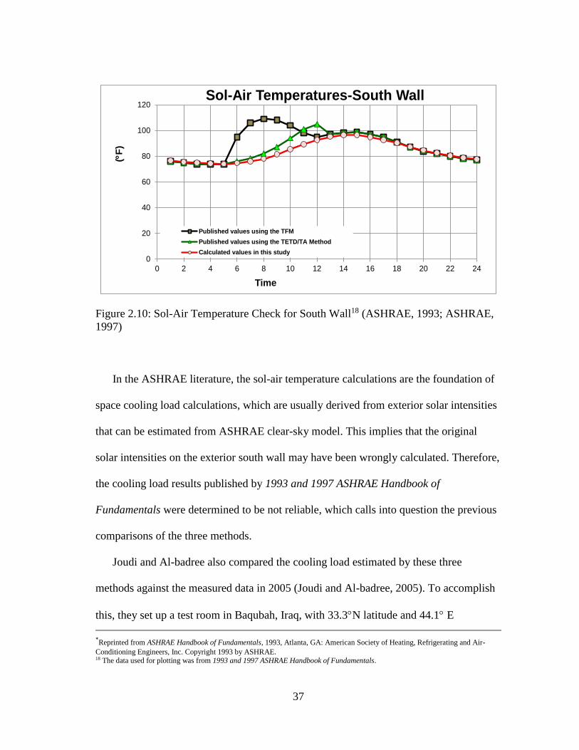
37
0
20
40
60
80
100
120
0 2 4 6 8 10 12 14 16 18 20 22 24
(F
)
Time
Sol-Air Temperatures-South Wall
Published values using the TFM
Published values using the TETD/TA Method
Calculated values in this study
Figure 2.10: Sol-Air Temperature Check for South Wall18 (ASHRAE, 1993; ASHRAE,
1997)
In the ASHRAE literature, the sol-air temperature calculations are the foundation of
space cooling load calculations, which are usually derived from exterior solar intensities
that can be estimated from ASHRAE clear-sky model. This implies that the original
solar intensities on the exterior south wall may have been wrongly calculated. Therefore,
the cooling load results published by 1993 and 1997 ASHRAE Handbook of
Fundamentals were determined to be not reliable, which calls into question the previous
comparisons of the three methods.
Joudi and Al-badree also compared the cooling load estimated by these three
methods against the measured data in 2005 (Joudi and Al-badree, 2005). To accomplish
this, they set up a test room in Baqubah, Iraq, with 33.3N latitude and 44.1 E
*Reprinted from ASHRAE Handbook of Fundamentals, 1993, Atlanta, GA: American Society of Heating, Refrigerating and Air-
Conditioning Engineers, Inc. Copyright 1993 by ASHRAE. 18 The data used for plotting was from 1993 and 1997 ASHRAE Handbook of Fundamentals.
38
longitude. The building had a medium weight with an air-conditioning unit installed to
control indoor dry bulb indoor temperatures to be constant at 26C (78.8 F). The hourly
outdoor dry bulb temperatures, indoor dry bulb temperatures and air velocities were
measured for May 21st, June 21st, July 21st, August 21st, and September 21st in 2004. The
peak cooling load estimations were then performed for the design days using the TFM,
the TETD/TA Method, the CLTD/SCL/CLF Method. Their study showed a large
difference between the measured and predicted cooling load for all three methods, which
were 36%, 33% and 40 % percent differences for the CLTD/SCL/CLF Method, the
TFM, and the TETD/TA Method, respectively. These comparisons were performed
using one type of building construction. In general, although this study had very
different results, it is viewed as an important reference rather than a final conclusion for
three method comparisons.
2.4.2 Comparisons among the HBM, the RTSM, and the Admittance Method
A comparison of cooling load calculation procedures published by ASHRAE/CIBSE
was also performed in ASHRAE Project RP-942, which resulted in four papers (Spitler
and Rees, 1998; Rees et al., 1998; Rees and Spitler, 1999; Rees et al., 2000). The focus
of this project compared the HBM, the RTSM and the admittance method.
In general, European countries use the admittance method for peak cooling load
calculations. It was first developed by A.G. Loudon (Loudon, 1968) at the Building
Research Station to calculate summertime temperatures in buildings, and later adopted
by the CIBSE in Guide A (originally, named IHVE Guide) in 1970. In the admittance
39
method, instead of just referencing the zone air temperature, the admittance method
relies on two nodes inside the building: the zone air temperature node and the
environmental temperature node, where the “environmental temperature node” is a
hypothetical node that was introduced by Loudon to take account of the effects of the
mean radiant temperature (MRT) on heat losses because the heat is transferred to the
surfaces of exposed panels by long-wave radiation from other room surfaces as well as
by convection from air. CIBSE also published a so called “cyclic” model to predict
dynamic heating and cooling loads of buildings (CIBSE, 2006). This cyclic model
includes both a steady-state and a fluctuation model, which assumes that all fluctuations
are sine waves with a period of 24 hours.
Spitler and Rees performed a quantitative comparison of the North American and
U.K. cooling load calculation procedures in 1998 (Spitler and Rees, 1998). The
comparison detailed all parameters and calculation tools that were used. In the same
year, Rees et al. published the results of the comparison of these three methods (Rees et
al., 1998). In their comparison over 7,000 combinations of tests were performed.
Compared to the HBM, they found that the RTSM significantly over-predicted the peak
cooling loads under the condition of large amounts of single-pane glazing, which
reached as high as a 37% difference. For other cases, the RTSM was generally well
behaved. The study also showed the admittance method over-predicted the peak cooling
load for heavy-weight cases, but under-predicted the peak cooling load for light weight
cases. One year later, in 1999, Rees and Spitler proposed a diagnostic test procedure for
building loads (Rees and Spitler, 1999). In this study, several tests were performed using
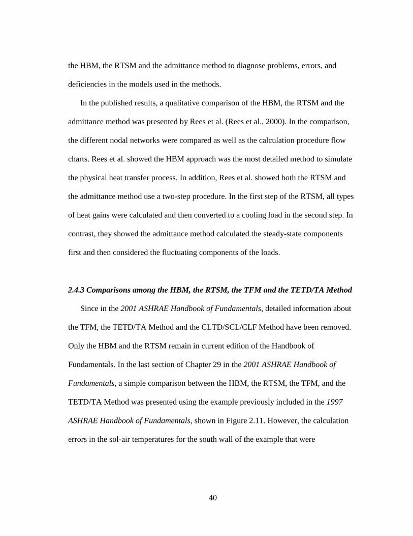
40
the HBM, the RTSM and the admittance method to diagnose problems, errors, and
deficiencies in the models used in the methods.
In the published results, a qualitative comparison of the HBM, the RTSM and the
admittance method was presented by Rees et al. (Rees et al., 2000). In the comparison,
the different nodal networks were compared as well as the calculation procedure flow
charts. Rees et al. showed the HBM approach was the most detailed method to simulate
the physical heat transfer process. In addition, Rees et al. showed both the RTSM and
the admittance method use a two-step procedure. In the first step of the RTSM, all types
of heat gains were calculated and then converted to a cooling load in the second step. In
contrast, they showed the admittance method calculated the steady-state components
first and then considered the fluctuating components of the loads.
2.4.3 Comparisons among the HBM, the RTSM, the TFM and the TETD/TA Method
Since in the 2001 ASHRAE Handbook of Fundamentals, detailed information about
the TFM, the TETD/TA Method and the CLTD/SCL/CLF Method have been removed.
Only the HBM and the RTSM remain in current edition of the Handbook of
Fundamentals. In the last section of Chapter 29 in the 2001 ASHRAE Handbook of
Fundamentals, a simple comparison between the HBM, the RTSM, the TFM, and the
TETD/TA Method was presented using the example previously included in the 1997
ASHRAE Handbook of Fundamentals, shown in Figure 2.11. However, the calculation
errors in the sol-air temperatures for the south wall of the example that were
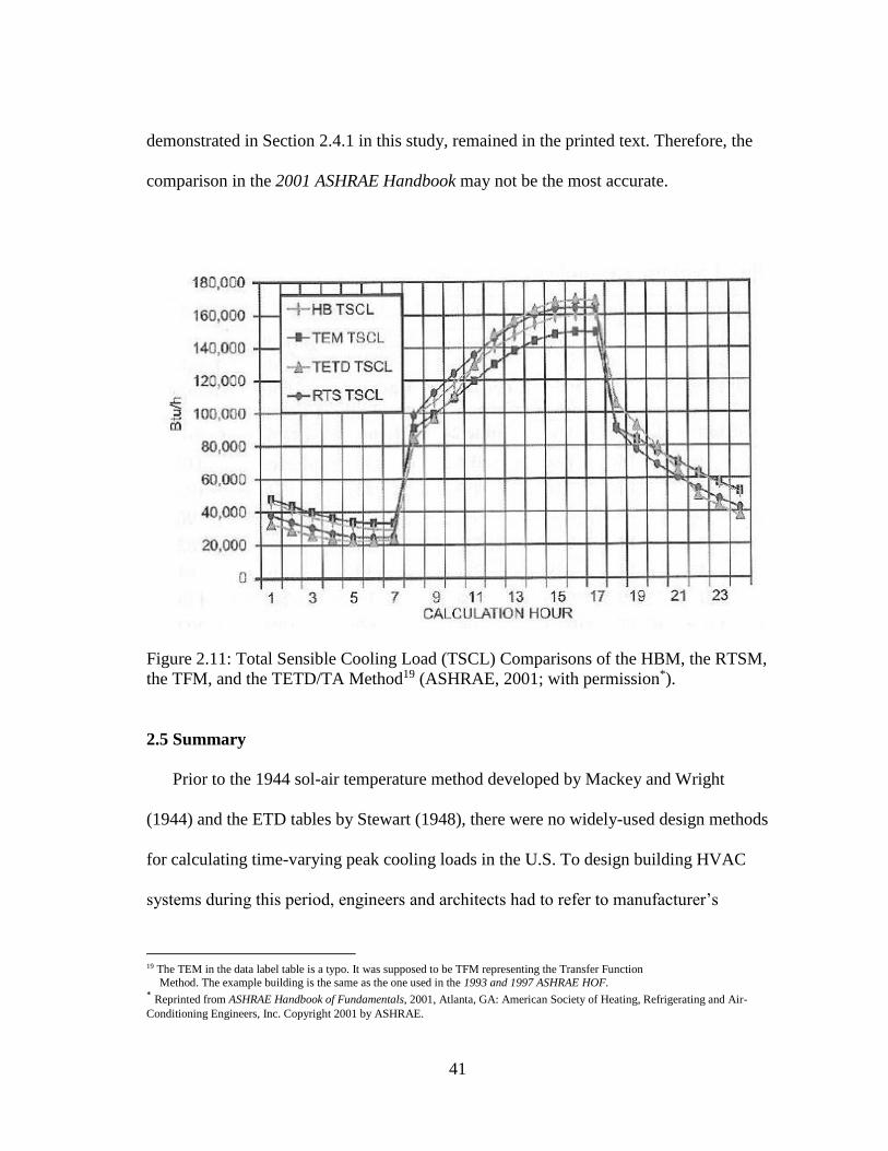
41
demonstrated in Section 2.4.1 in this study, remained in the printed text. Therefore, the
comparison in the 2001 ASHRAE Handbook may not be the most accurate.
Figure 2.11: Total Sensible Cooling Load (TSCL) Comparisons of the HBM, the RTSM,
the TFM, and the TETD/TA Method19 (ASHRAE, 2001; with permission*).
2.5 Summary
Prior to the 1944 sol-air temperature method developed by Mackey and Wright
(1944) and the ETD tables by Stewart (1948), there were no widely-used design methods
for calculating time-varying peak cooling loads in the U.S. To design building HVAC
systems during this period, engineers and architects had to refer to manufacturer’s
19 The TEM in the data label table is a typo. It was supposed to be TFM representing the Transfer Function
Method. The example building is the same as the one used in the 1993 and 1997 ASHRAE HOF. * Reprinted from ASHRAE Handbook of Fundamentals, 2001, Atlanta, GA: American Society of Heating, Refrigerating and Air-
Conditioning Engineers, Inc. Copyright 2001 by ASHRAE.
42
literature, textbooks, guidebooks or their own experiences, which varied widely. The
earliest textbooks include: Eugéne Péclet (1844), Hermann Rietschel (1894), Rolla
Carpenter (1896), Charles Paulding (1904), Frank Kidder (1906), John Allen (1935),
Charles Merrick Gay and Charles De Van Fawcett (1937). In addition, manufacturers
like Trane and Carrier developed and used their own methods, which were eventually
published (TRANE, 1938; Carrier, 1914). Interestingly, prior to 1944, building peak
heating load calculation methods primarily used “word formulas” to describe the
calculation procedure, which may be due in part to the difficulty and expense of type-
setting the complex formula in the published text. In the U.S., building peak cooling load
calculations began with the decrement factor by Alford et al. in 1939, which provided
the foundation for the sol-air temperature method later developed by Mackey and Wright
in 1944.
In 1948, Stewart developed the Equivalent Temperature Differentials table from the
sol-air temperature equations of Mackey and Wright, which resulted in the ETD tables
published in the 1951 ASHVE Guide and 1961 ASHRAE Guide and Data Book. The
ETD tables were the foundation of TETD/TA Method later introduced in 1967 ASHRAE
Handbook of Fundamentals.
The thermal response factor method was introduced by Mitalas and Stephenson in
1967, based on the previous work done by Nessi and Nisolle (1925), Hill (1957), and
Brisken and Reque (1956). In 1958, the heat balance and thermal network methods were
demonstrated by Buchberg (1958) for simulating a house on an analog computer as part
of an ASHRAE sponsored research project. In 1972, ASHRAE Task Group published
43
the TFM for calculating dynamic heat transfer, which laid the basis for the CLTD/CLF
Method that was later modified by Sowell (1988), Harries (1988), McQuiston (1988),
and Spitler (1993) to become the CLTD/SCL/CLF Method.
In 1993, Spitler et al. published the RTSM for dynamic peak cooling load
calculations. The RTSM served as a foundation for the residential RHB and RLF
methods developed by Barnaby in 2004. Finally, ASHRAE released its LOADS Toolkit,
developed by Professor Curtis Pedersen at the University of Illinois, which included
FORTRAN code for the HBM in 2001. Today, all five methods (i.e., TETD/TA Method,
TFM, CLTD/SCL/CLF Method, RTSM, HBM) remain in use in the industry. However,
only the HBM and RTSM are referenced in the ASHRAE Handbook of Fundamentals
since the 2001 edition.
Also, several studies were reviewed that compared the existing methods, including:
comparisons of the TFM, the TETD/TA and the CLTD/SCL/CLF; comparisons of the
HBM, the RTSM, and the admittance method; and comparisons of the HBM, the RTSM,
the TFM, and the TETD/TA Method. However, mistakes related to sol-air temperature
calculations were discovered by Al-Rabghi and Al-Johani as well as the current study.
Therefore, the comparison results may not be as reliable as once thought. In addition, in
the ASHRAE Handbook comparisons, the shown example was one building
configuration in one climate. No other cases were identified that presented results for
different climates. Therefore, there is a need to revisit and compare all five peak cooling
load methods.

44
CHAPTER III
METHODOLOGY
3.1 Overview
This Chapter presents details about the research methodology used for the current
study, which is shown in Figure 3.1. The methodology used in the current study is
composed of four tasks: a survey and interview; the RP-1117 base-case comparison; the
additional case-study comparison; and the proposed modifications to the
CLTD/SCL/CLF Method.
The survey and interview were performed to better understand the actual peak
cooling load design process used in the HVAC field. By surveying and interviewing the
HVAC field professionals, the use of the HBM, the RTSM, the TFM, the TETD/TA
Method, and the CLTD/SCL/CLF Method were reviewed, as well as the pros and cons
of each methodology.
Next, a quantitative analysis was performed to thoroughly compare the current five
methods using selected data from the published case studies from the ASHRAE RP-
1117 report. Base-case comparisons were then performed using as-built building
information in the report. In addition, an extended analysis of the TFM, the TETD/TA
Method, and the CLTD/SCL/CLF Method was performed. Furthermore, in order to
study fenestration heat gain impacts on the space sensible cooling loads predicted by the
five methods, fifteen additional study cases were designed and analyzed. Finally, an
update to the SCL tables was proposed to modify the CLTD/SCL/CLF Method, since the

45
fenestration heat gain model in the CLTD/SCL/CLF Method is out-of-date compared to
the RTSM.
3.2 Survey and Interview
The survey and interview process is shown in Figure 3.2. To begin with, a potential
participant list was obtained from the ASHRAE Houston Chapter. All candidates were
building design professionals who were active in the design field. Next, research
questions were developed for the survey form and the phone interview. The whole
process consisted of two parts: a written survey; and a phone interview. The written
survey form was intended to be a quick way to obtain a basic set of information. The
phone interview was designed to obtain additional details about the questions in the
written survey.
Before the survey was conducted, an approval from Institutional Review Board
(IRB) was obtained. The IRB submission included:
Contact list;
Designed survey form;
Designed interview questions;
Consent information sheet;
Recruitment email.
The approval letters are shown in Appendix A.

46
Once the IRB approval was received, a recruitment email was sent to each potential
candidate in the list. If the candidates were willing to participate in the study, the one-
page written survey form was sent to obtain the general survey information. After the
survey was performed, the participants were asked whether they were willing to
participate in a phone interview. If they answered yes, a 15-minute phone interview was
scheduled and the design interview questions were presented. The survey and interview
results were analyzed in the final step.

47
Survey and Interview
RP -1117 Base-Case Comparisons
Additional Case-Study Comparisons
Proposed Updates for
CLTD/SCL/CLF Method
Figure 3.1: Overview of Research Methodology
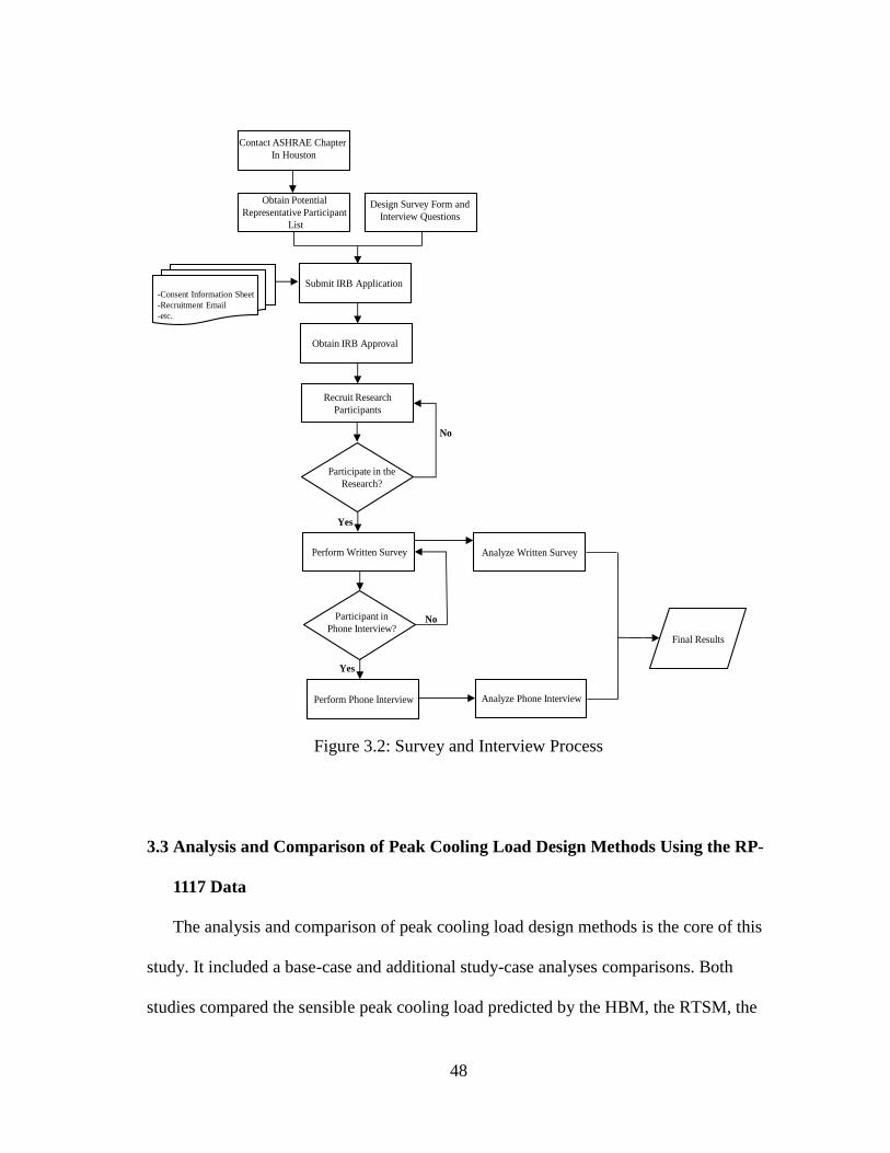
48
Contact ASHRAE Chapter
In Houston
Obtain Potential
Representative Participant
List
Design Survey Form and
Interview Questions
Submit IRB Application
Obtain IRB Approval
-Consent Information Sheet
-Recruitment Email
-etc.
Recruit Research
Participants
Participate in the
Research?
No
Perform Written Survey
Yes
Participant in
Phone Interview?No
Perform Phone Interview
Yes
Analyze Written Survey
Analyze Phone Interview
Final Results
Figure 3.2: Survey and Interview Process
3.3 Analysis and Comparison of Peak Cooling Load Design Methods Using the RP-
1117 Data
The analysis and comparison of peak cooling load design methods is the core of this
study. It included a base-case and additional study-case analyses comparisons. Both
studies compared the sensible peak cooling load predicted by the HBM, the RTSM, the

49
TFM, the TETD/TA Method, and the CLTD/SCL/CLF Method. In both analyses, only
the building envelope load was studied, which did not cover the effects of internal heat
gains, different HVAC system configuration, and plant. In all cases, one simplified case-
study building in the RP-1117 project was used to help identify differences in the
specific envelope components of the peak cooling load.
3.3.1 RP-1117 Base-Case Analysis and Comparisons of Cooling Load Methods
The base-case study uses the published data from the ASHRAE RP-1117 report and
additional data provided by contacting authors of RP-1117 report (Fisher, 2015). The
analysis and comparison procedure is shown in Figure 3.3.
3.3.1.1 HBM Validation Analysis
Since the ASHRAE RP-1117 project adopted the ASHRAE LOADS Toolkit as the
primary tool to perform the HBM analysis, it was determined that it was necessary to
verify the published simulation results in this report. Unfortunately, the first attempt to
replicate the analysis failed when using the published ASHRAE LOADS Toolkit CD
and associated source codes. So the author of RP-1117 report was contacted and a
separate FORTRAN code and data files used in the RP-1117 were provided (Fisher,
2015).
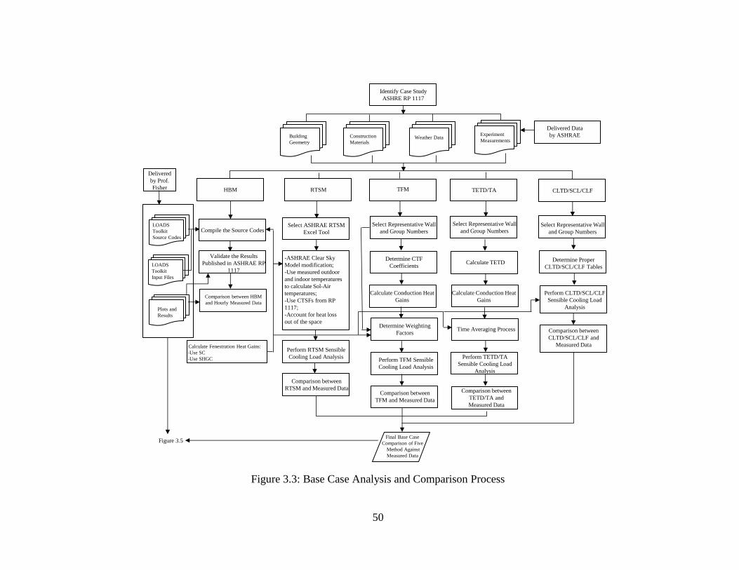
50
Identify Case Study
ASHRE RP 1117
Building
Geometry
Construction
MaterialsWeather Data
Experiment
Measurements
HBM RTSM TFM TETD/TA CLTD/SCL/CLF
Delivered Data
by ASHRAE
LOADS
Toolkit
Source Codes
LOADS
Toolkit
Input Files
Plots and
Results
Delivered
by Prof.
Fisher
Compile the Source Codes
Validate the Results
Published in ASHRAE RP
1117
Comparison between HBM
and Hourly Measured Data
Select ASHRAE RTSM
Excel Tool
-ASHRAE Clear Sky
Model modification;
-Use measured outdoor
and indoor temperatures
to calculate Sol-Air
temperatures;
-Use CTSFs from RP
1117;
-Account for heat loss
out of the space
Perform RTSM Sensible
Cooling Load Analysis
Comparison between
RTSM and Measured Data
Select Representative Wall
and Group Numbers
Determine CTF
Coefficients
Determine Weighting
Factors
Calculate Conduction Heat
Gains
Perform TFM Sensible
Cooling Load Analysis
Comparison between
TFM and Measured Data
Calculate Fenestration Heat Gains:
-Use SC
-Use SHGC
Calculate TETD
Select Representative Wall
and Group Numbers
Time Averaging Process
Perform TETD/TA
Sensible Cooling Load
Analysis
Comparison between
TETD/TA and
Measured Data
Select Representative Wall
and Group Numbers
Determine Proper
CLTD/SCL/CLF Tables
Calculate Conduction Heat
Gains
Perform CLTD/SCL/CLF
Sensible Cooling Load
Analysis
Comparison between
CLTD/SCL/CLF and
Measured Data
Final Base Case
Comparison of Five
Method Against
Measured Data
Figure 3.5
Figure 3.3: Base Case Analysis and Comparison Process

51
Once these were successfully compiled, the analysis was repeated and the results of the
RP-1117 report were reproduced.
In reviewing the HBM source codes, it was also found that the ASHRAE clear-sky
model had differences with the published models, which are the 1967 ASHRAE clear-
sky model (ASHRAE, 1967-2005) and 2009 clear-sky model (ASHRAE, 2009-2013).
The 1967 ASHRAE clear-sky model utilizes A, B, C coefficients and has two sets of
numbers have been found, which are shown in Table B.1 and Table B.2 in Appendix B.
The 2009 ASHRAE clear-sky model uses a different algorithm that is shown in Section
B.2.2 in Appendix B.
In addition, prior to the analysis, it was found that the published measured sensible
peak cooling load data was provided with 15-min interval. In order to compare the
measurements against other methods that provided the hourly sensible cooling load only,
the 15-min data was converted into hourly data.
3.3.1.2 RTSM Analysis
ASHRAE published a spreadsheet tool to perform the RTSM analysis (Spitler,
2009), which was adopted as the primary tool in this study. However, to adapt the tool
for the current study, several modifications were made to use actual measured indoor,
outdoor temperatures rather than the temperatures from peak design conditions that are
provided with the tool. Originally, the RTSM Visual Basic for Application (VBA)
source codes uses the 1967 ASHRAE clear-sky model with the second sets of
coefficients. Therefore, to be consistent with the HBM used in RP-1117, the first sets of
52
values were used in this study. In the RP-1117 report, the solar heat loss was calculated
and subtracted from the total solar heat gains, which was also included in the spreadsheet
tool. Finally, the sensible cooling load was estimated from this RTSM Spreadsheet Tool
and compared to the hourly measured data.
3.3.1.3 TFM Analysis
The accuracy of the TFM depends significantly on the how well representative wall
and roof group numbers that are selected by the peak load designer match the building
being studied. Using the building geometry and construction material layers defined in
the RP-1117 report, the proper group combinations were chosen for this study, as well as
the published default tables by ASHRAE so the Conduction Transfer Function
coefficients could be determined (ASHRAE, 1997). Next, the conduction heat gains
were calculated.
During this process, it was also noticed that the last published version of TFM still
recommended using the Shading Coefficient (SC) to calculate fenestration heat gains
(ASHRAE, 1997). Starting from the 2001 ASHRAE Handbook of Fundamentals, the
TFM was eliminated from the Handbook and replaced with the HBM and the RTSM
peak cooling load calculation methods. As the RTSM was developed, the fenestration
model was updated to use the new angular Solar Heat Gain Coefficients (SHGC) instead
of the older SC method. A comparison of the two fenestration models is provided in
Appendix C. In this study, the most recent SHGC fenestration heat gain model was used
53
in the TFM analysis, which could provide more precise estimation for solar heat gains
coming into the space.
After all the heat gains were calculated, the next step was to determine the
corresponding weighting factors, which were obtained through TFMTAB.EXE
(McQuiston and Spitler, 1992). The software is shown in Appendix F. Finally, the
sensible cooling load using the TFM was analyzed. The comparisons between the TFM
and measured data were then performed.
3.3.1.4 TETD/TA Method Analysis
In the same fashion as the TFM, once the wall and group combination group
numbers were determined, the hourly TETD was calculated using the corresponding
time lag and decrement factor (ASHRAE, 1997). The conduction heat gains were then
calculated by multiplying TETD by the UA. Next, the time averaging process was
performed. Finally, the sensible cooling predicted by the TETD/TA Method was
calculated and the comparison was made against measured cooling load.
3.3.1.5 CLTD/SCL/CLF Method Analysis
Similarly, the wall and roof group numbers were selected for the CLTD/SCL/CLF
Method. The best selection was made to better represent the current case study. The
CLTD and SCL tables for the correct latitude and month were generated by CLTDTAB.
EXE program (McQuiston and Spitler, 1992). Additional details are provided in

54
Appendix H. Finally, the sensible cooling load using CLTD/SCL/CLF Method was
calculated and the comparison was made against the measured data.
3.3.1.6 Comparison of All Methods Against the Measured Data
With all individual peak cooling load estimated, the final comparisons between the
HBM, the RTSM, the TFM, the TETD/TA Method, and the CLTD/SCL/CLF Method
were performed.
3.3.2 Additional Case-Study Analysis and Comparisons of the Cooling Load Methods
To further understand the influence of glazing area on the sensible peak cooling load
estimation by all five methods, fifteen additional test cases were used in the comparison.
The procedure is shown in Figure 3.4, starting with the entry of all information for each
case for the HBM, the RTSM, the TFM, the TETD/TA Method, and the
CLTD/SCL/CLF Method. In all comparisons, the sensible peak cooling load by the
HBM was regarded as the baseline to be compared against.
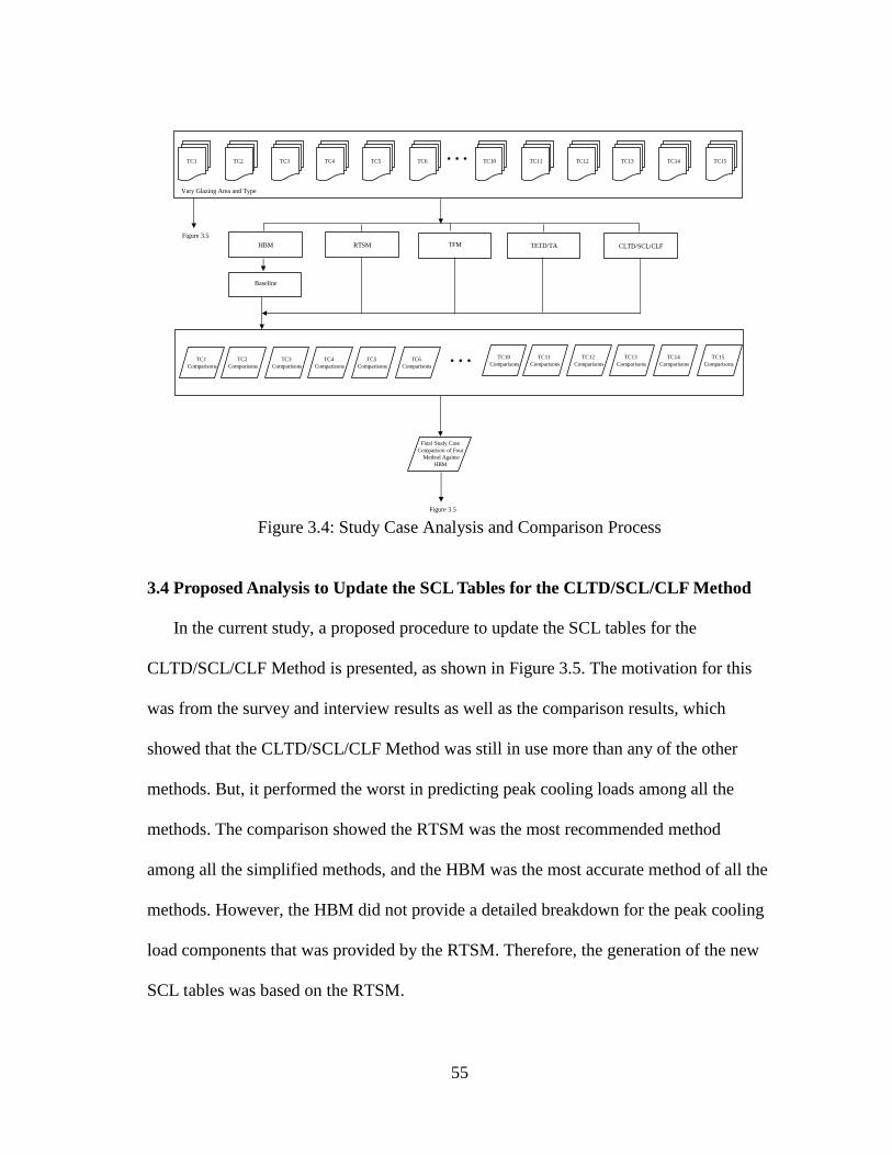
55
TC1 TC2 TC3 TC4 TC5 TC6 TC10 TC11 TC12 TC13 TC14 TC15Vary Glazing Area and Type
HBM RTSM TFM TETD/TA CLTD/SCL/CLF
Baseline
TC1
Comparisons
TC2
Comparisons
TC3
Comparisons
TC4
Comparisons
TC5
Comparisons
TC6
Comparisons
TC10
Comparisons
TC11
Comparisons
TC12
Comparisons
TC13
Comparisons
TC14
Comparisons
TC15
Comparisons
Final Study Case
Comparison of Four
Method Against
HBM
Figure 3.5
Figure 3.5 Figure 3.4: Study Case Analysis and Comparison Process
3.4 Proposed Analysis to Update the SCL Tables for the CLTD/SCL/CLF Method
In the current study, a proposed procedure to update the SCL tables for the
CLTD/SCL/CLF Method is presented, as shown in Figure 3.5. The motivation for this
was from the survey and interview results as well as the comparison results, which
showed that the CLTD/SCL/CLF Method was still in use more than any of the other
methods. But, it performed the worst in predicting peak cooling loads among all the
methods. The comparison showed the RTSM was the most recommended method
among all the simplified methods, and the HBM was the most accurate method of all the
methods. However, the HBM did not provide a detailed breakdown for the peak cooling
load components that was provided by the RTSM. Therefore, the generation of the new
SCL tables was based on the RTSM.

56
As previously mentioned in the Section 2.3.4, in 2006, a spreadsheet tool was
proposed by TC 4.1 volunteers to generate the custom CLTD and CLF tables using the
RTSM (Bruning, 2016). In this tool, for the window cooling load calculation, a window
CLF table was used to combine the cooling load from both conduction and solar heat
gains, which eliminated the SCL tables.
Differently, the current study approach focuses on updating the SCL tables only to
improve the accuracy of the CLTD/SCL/CLF Method. This is because the solar cooling
load calculation by ASHRAE CLTD/SCL/CLF Method uses the published SCL tables
and the Shading Coefficient (SC) instead of the Solar Heat Gain Coefficient (SHGC)
method. Therefore, there is a need to update the SCL tables to reflect the more accurate
values from the SHGC fenestration heat gain model. To accomplish this, a new term
called “SCLModified” was derived from the fenestration solar heat gain calculation using
the RTSM principles. This resulted in a new equation to calculate the solar cooling load
by multiplying the SCLModified by window area time the product of the normal SHGC and
the Interior Attenuation Coefficients (IAC). The modified SCL tables were then updated
using the same format of the original SCL tables. An example of how to use the potential
ways to generate the SCL tables was also provided.
In this analysis, three representative cases were chosen, which included a base case
(single-pane clear glazing), a TC6 case (double-pane clear glazing), and a TC12 case
(triple-pane clear glazing). To accomplish this analysis, all information was loaded into
the ASHRAE RTSM Spreadsheet Tool. Next, in the same fashion as the original SCL
tables, all nine orientations of the windows were analyzed, including N, NE, E, SE, S,

57
SW, W, NW, and Horizontal. The solar cooling load from both the beam and diffuse
solar heat gains were then calculated with the RTSM tool. The SCL was next determined
by dividing the hourly sensible cooling load by the surface area and normal SHGC.
Finally, the new SCL numbers replaced the old SCL values and the modified sensible
cooling load results were obtained.
Conclusions from
Survey/Interview, Base Case
Comparisons, and 15 Study Case
Comparisons
Review
Fenestration Heat
Gains Calculated
by SHGC
Review Original
CLTD/SCL/CLF
Methodology
Adopt ASHRAE RTSM
Excel ToolBase Case
Information
TC 6
Information
TC 12
Information
Perform Solar Cooling
Load by Using RTSM
Generate SCL Tables
Base
Case
TC 6 TC 12
Updated Base Case
Sensible Cooling Load
Updated TC 6
Sensible Cooling Load
Updated TC 12
Sensible Cooling Load
Final Results for Modified
CLTD/SCL/CLF Method
Figure 3.2, Figure 3.3, Figure 3.4
Figure 3.4
Figure 3.5: Procedure of CLTD/SCL/CLF Method Updates

58
CHAPTER IV
RESULTS OF THE STUDY
This chapter includes three parts of the results:
-Part I Results of survey and interview;
-Part II Base-case analysis and comparison of peak cooling load design methods;
- Part III Additional case-study comparison of the peak cooling load design methods.
4.1 Part I: Results of Survey and Interview
4.1.1 Overview
This section presents the results of a survey and interview process regarding the use
of building peak cooling load calculation methods in the design of today’s commercial
buildings. After the IRB approval20, the procedures used in the survey and interview
process were conducted in two phases. In Phase One, the selected candidates were asked
to fill-out a one-page survey form to gather general information about the participants,
such as: their knowledge background; types of buildings they have designed; the
methods that were used to design the buildings, etc. In Phase Two, if the candidates were
willing to continue, a 15-minute phone interview was scheduled to discuss the
advantages and disadvantages of the different peak cooling load design methods and the
tools that are being used in the field with each participant.
Originally, thirty-one candidates were selected, who were representative of HVAC
design professionals in the U.S. These candidates were invited to participate in the study
20 The IRB approval letters are shown in Appendix A.

59
through the ASHRAE Chapter in Houston, TX. Eleven candidates agreed to participate
in the survey study (Phase One) and nine candidates agreed to perform both the survey
and interview (Phase One + Phase Two). The name of candidates were coded as Selected
Field Professional (SFP) and kept confidential, in compliance with IRB requirements.
4.1.2 Survey Results
The pre-designed one-page survey was sent to each SFP candidate through the
recruitment email (shown in Figure 4.1), which contained eight questions.
4.1.2.1 Questions 1-3: SFP Knowledge Background
Questions 1-3 were designed to acquire information about the participants’
knowledge background. Nine out of eleven participants had a general engineering
background, and the remaining had an architectural engineering background. The years
of experience in designing actual building or HVAC systems ranged from 4 to 42 years.
Ten out of eleven participants have PE licenses. Two out of ten not only have PE
licenses, but also have LEED/Certified Commission Authority certificates. One
participant does not have a PE license.

60
Figure 4.1: Designed Survey Form
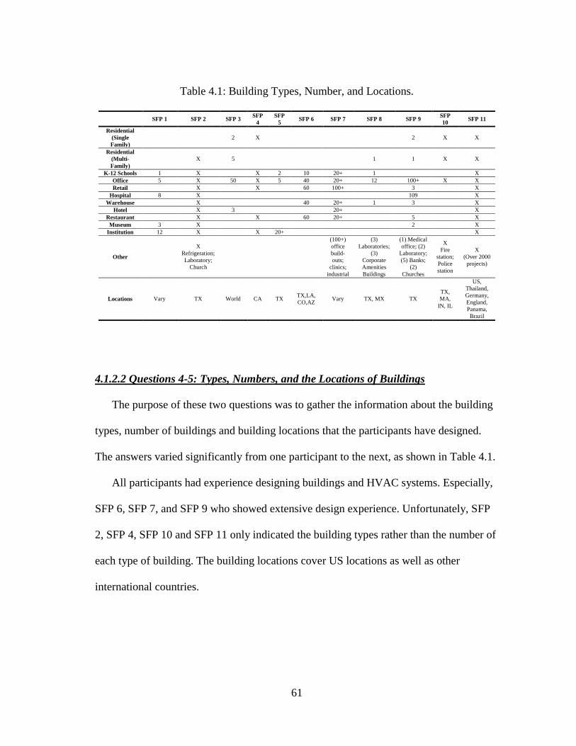
61
Table 4.1: Building Types, Number, and Locations.
SFP 1 SFP 2 SFP 3 SFP
4
SFP
5 SFP 6 SFP 7 SFP 8 SFP 9
SFP
10 SFP 11
Residential
(Single
Family)
2 X 2 X X
Residential
(Multi-
Family)
X 5 1 1 X X
K-12 Schools 1 X X 2 10 20+ 1 X
Office 5 X 50 X 5 40 20+ 12 100+ X X
Retail X X 60 100+ 3 X
Hospital 8 X 10⁹ X
Warehouse X 40 20+ 1 3 X
Hotel X 3 20+ X
Restaurant X X 60 20+ 5 X
Museum 3 X 2 X
Institution 12 X X 20+ X
Other
X
Refrigeration;
Laboratory;
Church
(100+)
office
build-
outs;
clinics;
industrial
(3)
Laboratories;
(3)
Corporate
Amenities
Buildings
(1) Medical
office; (2)
Laboratory;
(5) Banks;
(2)
Churches
X
Fire
station;
Police
station
X
(Over 2000
projects)
Locations Vary TX World CA TX TX,LA,
CO,AZ Vary TX, MX TX
TX,
MA,
IN, IL
US,
Thailand,
Germany,
England,
Panama,
Brazil
4.1.2.2 Questions 4-5: Types, Numbers, and the Locations of Buildings
The purpose of these two questions was to gather the information about the building
types, number of buildings and building locations that the participants have designed.
The answers varied significantly from one participant to the next, as shown in Table 4.1.
All participants had experience designing buildings and HVAC systems. Especially,
SFP 6, SFP 7, and SFP 9 who showed extensive design experience. Unfortunately, SFP
2, SFP 4, SFP 10 and SFP 11 only indicated the building types rather than the number of
each type of building. The building locations cover US locations as well as other
international countries.

62
4.1.2.3 Questions 6-7: Peak Load Design Methods That Have Been Used or Are Being
Used
Those two questions were intended to determine what design methods the
participants knew about, and/or were/being in use. The first question revealed how many
methods each participant was familiar with. The second question inquired about which
methods the participants were using.
Nine out of eleven participants had used the CLTD/SCL/CLF Method, and four
people were continuing to use it. Five of the participants indicated that they had used the
RTSM, and only three were currently using the method. Four out of the eleven
participants had used the TETD/TA Method and three were currently using it. Three of
the participants had used the HBM. Two were currently using it. Finally, only one of the
participants indicated that he had used TFM. None of the participants were currently
using the method.
The results showed most SFPs were familiar with the CLTD/SCL/CLF Method, the
RTSM, and the TETD/TA Method. It was also found that the CLTD/SCL/CLF Method
was the most popular method that is currently being used (four participants), followed by
the TETD/TA Method (three participants), the RTSM (three participants) and HBM (two
participants).
4.1.2.4 Question 8: Software Used in the Peak Load Design Process
From the survey results, ten out of the eleven participants are using the TRACE
software (Trane, 2010), which contains the TETD/TA Method, the CLTD/SCL/CLF

63
Method, and the RTSM. Five participants use Elite Software (Elite Software, 2016).
Three participants used spreadsheets that they had prepared. One participant uses the
HAP software (Carrier, 2003). There are also participants using building energy
simulation software to perform peak load calculations. Two of these participants used
eQuest (James J. Hirsch & Associates, 2010). One used DOE-2 (Winkelmann et al.,
1993) and the other chose to use the Ener-Win software (Degelman and Soebarto, 1995).
4.1.3 Interview Results
The purpose of the interview process was to have an opportunity to talk to the SFPs
to further understand the advantages and disadvantages of the methods that they are
using and the design issues and difficulties that they were facing and coping with.
A phone interview was scheduled with each SFP who was willing to participate.
Among the eleven, nine SFPs agreed to be interviewed. The phone interview was
conducted in a quiet conference room at the Energy Systems Laboratory. Each phone
interview lasted approximately 15 minutes. During the interview, pre-designed questions
were used, as shown in Figure 4.2. The answers from the participating SFPs were
manually transcribed. Once each phone interview was finished, a summary of all
answers was drafted. The draft summaries were sent to each SFP for review. The
interview results were then finalized after the comments were received from the
participating SFPs. One of the nine SFPs did not provide comments on the draft
summaries.

64
Figure 4.2: Designed Interview Questions

65
4.1.3.1 Question 1: The Primarily Designed Building Type
The purpose of this question was to understand the building types that SFPs are
familiar with and have experience in designing. Four out of the nine SFPs primarily
design commercial buildings. Three of the nine participants indicated designing office
buildings only. One mentioned designing fire and police stations. The last SFP did not
mention the specific building types they had designed, but did mention that over 2,000
projects had been designed.
4.1.3.2 Question 2: The Aspects of HVAC Design and Step-by-Step Design Process
The main focus of this question was to explore the actual design process used in the
industry when engineers design a building. Despite differences in the details, all SFPs
provided similar design procedures as follows:
1) The building owner brings a description and requirement to the
responsible architect(s).
2) The architect(s) prepare the conceptual design and send the building plans
to the engineers, such as the building envelope information.
3) The engineers perform load calculations, select system types, decide
system layout, and design the electrical, plumbing, fire protection, etc.
4) Finally, the engineers prepare all related documents, specifications, and
notes.
66
From this general procedure, it was clear that one of the engineer’s major duties was
to perform the peak heating and cooling load calculations, after the architect had
performed the preliminary design of the building.
4.1.3.3 Question 3: Tools and Methodology Used in the Peak Load Design Process
The primary tools mentioned in the interview include the TRACE, IES, HAP, and
Elite software, which were used to perform the load calculations. The calculation
methodologies used by the tools included the CLTD/SCL/CLF Method, the TETD/TA
Method, the HBM, and finally the RTSM. The TFM was not mentioned by any of the
nine SFPs.
4.1.3.4 Question 4: The Advantages and Disadvantages of the Peak Load Design
Methods
Five out of the nine SFPs said they used the CLTD/SCL/CLF Method because it is
user friendly and easy-to-use as well as the fact that it provides a detailed breakdown of
each cooling load component. However, one SFP mentioned the CLTD/SCL/CLF was
their least favorite method because it was too simplified and contained too many
assumptions about the CLTD/SCL/CLF tables.
Three out of the nine SFPs discussed the RTSM. Two of the SFPs gave very
different views. One said the RTSM would be used when designing LEED building and
the other said RTSM was rarely used even though it is a more accurate method
compared to others. The last SFP claimed the RTSM was their favorite method, because

67
it was derived from the HBM. This SFP said that for a typical building, the RTSM
results were very close to results from the HBM.
4.1.3.5 Question 5: How was the Method/Tool Learned
Most of the SFPs learned the original methodologies in school, but mastered the
software at work.
4.1.3.6 Question 6: Whether the Current Tools/Methods are Good Enough for
Designing Today’s Commercial Buildings in the U.S.
All SFPs said yes to this question. One SFP suggested that sometimes they needed to
change the design inputs when using the tools to better match a particular building.
4.1.3.7 Question 7: Building Features that are not Covered in the Current Methods
All SFPs indicated that the typical features found in today’s building are all covered
in the current methods. However, some high-performance features were not covered,
including: double-skin façades, renewable energy systems, chilled beams, radiant floor
slabs, and comfort control.
4.1.3.8 Question 8: Future Trend of Peak Load Design Method
All the SFPs agreed that simulation will be used more and more in the future and the
manual calculation would be performed only as a quick check. Two SFPs think that the
Building Information Modeling (BIM) software, such as Revit, will be the future tool
68
that can integrate the architectural design with load calculation.
4.1.3.9 Question 9: Other Issues/Challenges
Each SFP has their own opinions about this question according to their working
experience, including:
1) More attention should be given to controls and equipment efficiency;
2) Cooperation with architects during the design process was important ;
3) Challenges in peak load diversities and non-well mixed spaces;
4) Changes in climate zone definitions and building codes;
5) Humidity control during the design process;
6) Quality input data for the simulation.
4.1.4 Summary of Survey and Interview Analysis
In summary, the survey and interview of the Selected Field Professionals (SFPs)
showed that the CLTD/SCL/CLF Method was still widely used today. This method is
implemented in the TRACE software and is felt to be user friendly. The HBM was felt to
be the most accurate method. However, it has no breakdown for each cooling load
component and it has complexities that make it difficult to use. Among the current study
pool, only three SFPs mentioned the RTSM, which was the only simplified method
contained in the current ASHRAE Handbook of Fundamentals (ASHRAE, 2013a).
However, two of the SFPs rarely used this method since other easy-to-use methods were
still available and continued to perform well for them. The TETD/TA Method was still

69
used during the peak load design phase. However, none of the SFPs used the TFM for
their designs.
4.2 Part II: Base-Case Analysis and Comparison of Peak Cooling Load Design
Methods
4.2.1 Overview
This section presents a comparison of the five peak cooling load calculation methods
for the selected base case study. The current five peak load design methods are: the Heat
Balance Method (HBM); the Radiant Time Series Method (RTSM); the Transfer
Function Method (TFM); the Total Equivalent temperature Difference/Time Averaging
Method (TETD/TA); and the Cooling Load Temperature Difference/Solar Cooling
Load/Cooling Load Factor Method (CLTD/SCL/CLF).
For a typical building, all types of heat gains can enter a space. The convective heat
gains directly impact the cooling load, while, the radiative heat gains are first absorbed
by the interior structures and then convected to the zone air in the space after a time
delay, as shown in Figure 4.3.
The HBM is considered the most accurate method among all the methods. As a one-
step method, it utilizes an iterative procedure to perform the heat balance calculations on
each interior and exterior surface. Due to its complexity, the users need to rely on
software to run a peak cooling load analysis with the HBM.
The other four methods are simplified methods. The CLTD/SCL/CLF Method was
developed as a manual one-step calculation procedure. The CLTD is used to calculate

70
the space cooling load from conduction heat gains through external surfaces, including
walls, roofs, and windows. The SCL are applied to obtain the space cooling load from
the solar heat gains through the fenestration. The CLF is only used when internal heat
gains are involved.
The RTSM, the TFM and the TETD/TA Method are all two-step methods. They all
use the concept of sol-air temperatures to combine the solar radiation effects on the
external surfaces together with the one-dimensional heat conduction process. The
differences among them are the way they calculate the conduction heat gains through the
exterior opaque surfaces and the procedure to convert the heat gains into the space
cooling loads. As shown in Figure 4.3, the conduction heat gains for opaque surfaces can
be determined using the Periodic Response Factors (PRFs)/Conduction Time Series
Factors (CTSFs) of the RTSM, Conduction Transfer Functions (CTFs) of the TFM, or
Total Equivalent Temperature Difference (TETD) of the TETD/TA Method. In order to
calculate the space cooling load, the RTSM simply applies Radiant Time Factors (RTFs)
to the radiative heat gains, while the TFM uses Room Transfer Functions (also named
Weighting Factors) to calculate the space cooling load. The TETD/TA Method averages
all the heat gains according to a selected time period that is subjective by designers.

71
Heat GainsCooling
Load
Furnishings,
Structure, Variable
Heat Storage
Heat
Extraction
Convection
RadiationConvection
(with time delay)
TETD Time Averaging Process (TA)TETD/TA Method
CTF Room Transfer Function (RTF/WF)TFM
PRF/CTSF Radiant Time Factor (RTF)RTSM
Heat Balance Procedure
CLTD/SCL/CLFCLTD/SCL/CLF Method
HBM
Minor Room
Temperature Swing
Figure 4.3: Peak Cooling Load Design Method Comparison (Adapted from ASHRAE
Handbook of Fundamentals)
4.2.2 Selection of the Case Study Site
In order to test the peak cooling load methods, it is necessary to either construct a
test bench with needed instruments or search for a previously published case study with
measured cooling load data. Unfortunately, considering the cost and time efforts,
constructing a new test bench facility was not an option. Therefore, it was necessary to
look for a suitable commercial building that had already been built.
Several complications were encountered during the case selection process:
Typical commercial buildings do not have sub-metering. Therefore, it is
difficult to separate the measured building envelope load and measured
HVAC system load from the total energy consumptions. This was a major
concern. For a typical building, the measured energy consumption is
obtained through the utility offices. The energy consumption in the utility

72
bills usually reflects the combined building envelope and system loads,
which may result in an inaccurate validation process. Therefore, more time
and costs were needed to obtain the measured data just for building
envelope load.
Typical commercial buildings are too complex. Since the current study
focuses on space cooling loads estimated by different load calculation
methodologies, the result discrepancies were expected to come from the
methodologies only. Unfortunately, the complexity of the most buildings
introduces unwanted factors that can influence cooling load differences
beyond the intended measurement range. Therefore, a simple building was
desired for this study.
Typical commercial buildings include high-performance features to lower
the energy consumption and costs. Unfortunately, the current published
methods cannot model certain high-performance features that are
implemented in such buildings and become part of the building envelope,
including: PV panels serving as building wall and roof materials; active
windows; double envelope façades; phase-change materials; and ground-
coupling features.
After careful consideration, the published data used in ASHRAE RP-1117 project
(Fisher and Spitler, 2002) was selected to avoid the complications mentioned above. The
test site in the RP-1117 study is located in Stillwater, Oklahoma. At the site, two, two-

73
story buildings are used in the experiments, with the HVAC system installed in the first
floor of each building. The room on the second floor is the target to be tested, where the
cooling load analysis was performed. One building is a heavy-weight construction and
the other building is a light-weight construction. This case study was chosen so that the
difference in the cooling loads would reflect the thermal mass differences between the
two buildings. In each building, single-pane clear glass windows (6.45 m2) were
mounted on each side of the south and west walls, which represented the worst types of
windows.
Several test cell configurations were studied in the ASHRAE RP-1117 report,
including: a base configuration; a drop ceiling; carpet; blinds; furniture; and different
office configurations. For each test cell configuration, base and tuned models21 were
developed. Since the duplication of all previous tests was not the intention of the current
study, only the tuned configuration of both heavy-weight and light-weighted building
cases was selected for cooling load design method comparisons.
The tuned model used the measured global horizontal solar radiation to calculate the
direct normal solar radiation, compared to the base model, which utilized the 1967
ASHRAE clear-sky model22 that calculates normal direct solar radiation by using A and
B coefficients, shown in Appendix B.
In the tuned model, the direct normal solar radiation DNE is given by (Fisher and
Spitler, 2002),
21 Tuned models were established using measured outside dry bulb temperatures, indoor dry-bulb temperatures and global horizontal
solar radiation. More details can be found in ASHRAE RP-1117 report. 22 Appendix B details the 1967 ASHRAE Clear-Sky Model.

74
cos
THDN
z
EE
C
(4.1)
where,
THE : measured global horizontal solar radiation, W/m2;
C : ASHRAE clear-sky model coefficients;
cos z : cosine of solar zenith angle ( z ).
The model used the following measured weather (Figure 4.4):
Outdoor air temperatures (C), Tdb;
Indoor air temperatures (C), Tin-Heavy and Tin-Light;
Global solar radiation (W/m2);
Wind speed (m/s) and wind direction (degree).
The original data represented data averaged over a 5-min period. Therefore, in order
to simulate the hourly cooling load, the data was converted to a one-hour interval, as
shown in Figure 4.4. Besides the measurements mentioned above, the room supply
temperature, room return temperature and system volumetric flow rate were measured to
calculate the cooling loads.
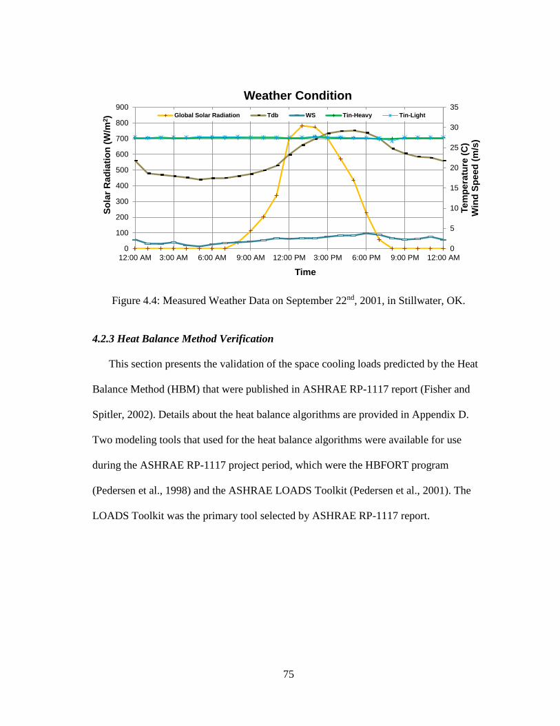
75
0
5
10
15
20
25
30
35
0
100
200
300
400
500
600
700
800
900
12:00 AM 3:00 AM 6:00 AM 9:00 AM 12:00 PM 3:00 PM 6:00 PM 9:00 PM 12:00 AM
Te
mp
era
ture
(C
)W
ind
Sp
ee
d (
m/s
)
So
lar
Ra
dia
tio
n (
W/m
2)
Time
Weather Condition
Global Solar Radiation Tdb WS Tin-Heavy Tin-Light
Figure 4.4: Measured Weather Data on September 22nd, 2001, in Stillwater, OK.
4.2.3 Heat Balance Method Verification
This section presents the validation of the space cooling loads predicted by the Heat
Balance Method (HBM) that were published in ASHRAE RP-1117 report (Fisher and
Spitler, 2002). Details about the heat balance algorithms are provided in Appendix D.
Two modeling tools that used for the heat balance algorithms were available for use
during the ASHRAE RP-1117 project period, which were the HBFORT program
(Pedersen et al., 1998) and the ASHRAE LOADS Toolkit (Pedersen et al., 2001). The
LOADS Toolkit was the primary tool selected by ASHRAE RP-1117 report.

76
4.2.3.1 ASHRAE LOADS Toolkit Review
The LOADS Toolkit CD was originally distributed by ASHRAE in 2001. The CD
includes source code written in FORTRAN 90. To be able to run the LOADS Toolkit,
the following files are needed,
The executable: SuccessiveSub.exe
The input file: in.idf
The object definition file: Toolkit.idd
The executable file provided by the RP-1117 report was generated by a FORTRAN
compiler that used FORTRAN source code with all FORTRAN libraries. To run this,
one needs to make sure all the above files are in the same folder. Running the .exe file
gives the following output files:
Audit.out
Toolkit.out
Toolkit.err
where the cooling load calculation results are contained in the Toolkit.out file.
4.2.3.1.1 Outside Surface Heat Balance
Three heat transfer processes are engaged in the outside surface heat balance
calculations, which include: the outside air convection; the absorbed incident solar; and
the long-wave radiation exchange.
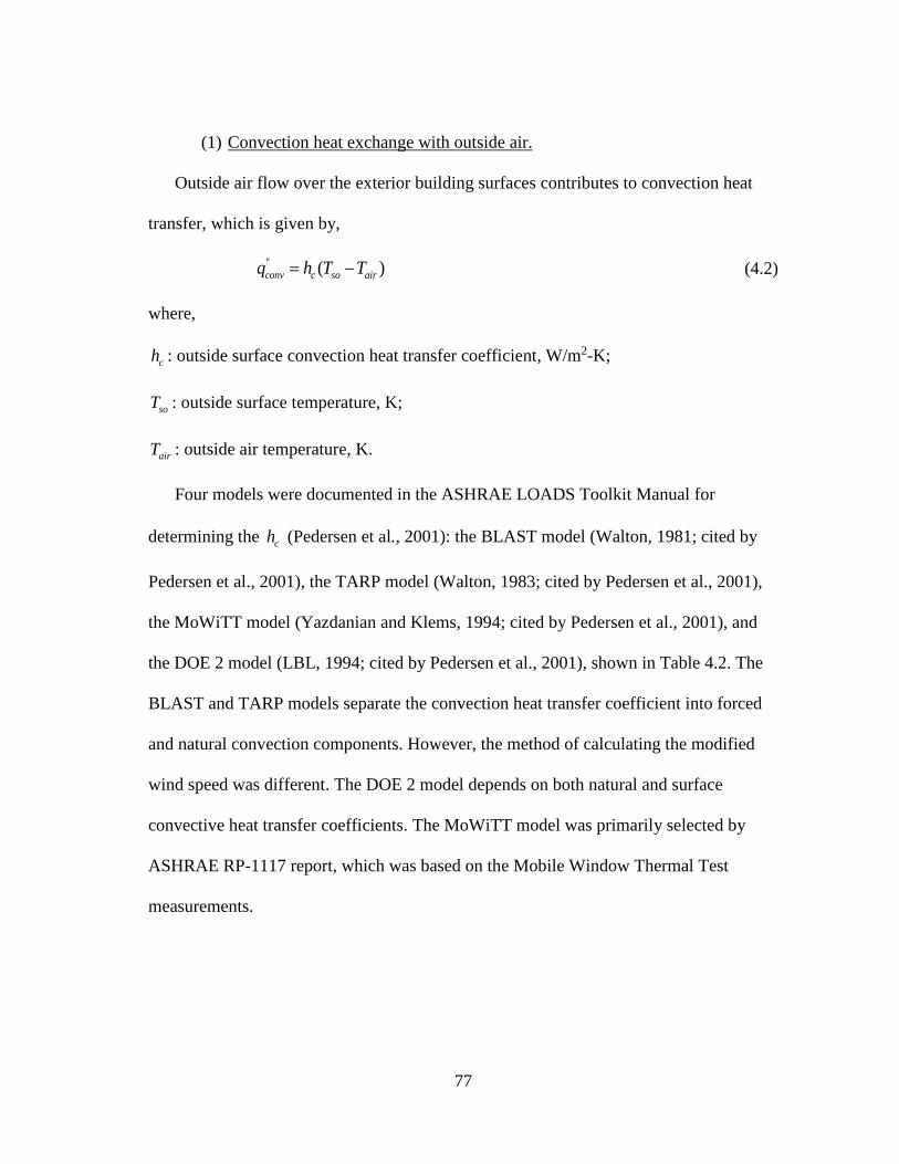
77
(1) Convection heat exchange with outside air.
Outside air flow over the exterior building surfaces contributes to convection heat
transfer, which is given by,
" ( ) conv c so airq h T T (4.2)
where,
ch : outside surface convection heat transfer coefficient, W/m2-K;
soT : outside surface temperature, K;
airT : outside air temperature, K.
Four models were documented in the ASHRAE LOADS Toolkit Manual for
determining the ch (Pedersen et al., 2001): the BLAST model (Walton, 1981; cited by
Pedersen et al., 2001), the TARP model (Walton, 1983; cited by Pedersen et al., 2001),
the MoWiTT model (Yazdanian and Klems, 1994; cited by Pedersen et al., 2001), and
the DOE 2 model (LBL, 1994; cited by Pedersen et al., 2001), shown in Table 4.2. The
BLAST and TARP models separate the convection heat transfer coefficient into forced
and natural convection components. However, the method of calculating the modified
wind speed was different. The DOE 2 model depends on both natural and surface
convective heat transfer coefficients. The MoWiTT model was primarily selected by
ASHRAE RP-1117 report, which was based on the Mobile Window Thermal Test
measurements.
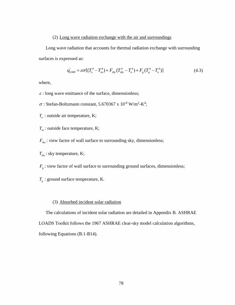
78
(2) Long wave radiation exchange with the air and surroundings
Long wave radiation that accounts for thermal radiation exchange with surrounding
surfaces is expressed as:
" 4 4 4 4 4 4[( ) ( ) ( )] LWR o so sky sky o g g oq T T F T T F T T (4.3)
where,
: long wave emittance of the surface, dimensionless;
: Stefan-Boltzmann constant, 5.670367 x 10⁻⁸ W/m2-K4;
oT : outside air temperature, K;
soT : outside face temperature, K;
skyF : view factor of wall surface to surrounding sky, dimensionless;
skyT : sky temperature, K;
gF : view factor of wall surface to surrounding ground surfaces, dimensionless;
gT : ground surface temperature, K.
(3) Absorbed incident solar radiation
The calculations of incident solar radiation are detailed in Appendix B. ASHRAE
LOADS Toolkit follows the 1967 ASHRAE clear-sky model calculation algorithms,
following Equations (B.1-B14).
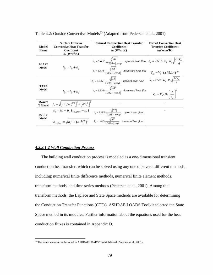
79
Table 4.2: Outside Convective Models23 (Adapted from Pedersen et al., 2001)
Model
Name
Surface Exterior
Convective Heat Transfer
Coefficent
hc (W/m2K)
Natural Convecctive Heat Trasnfer
Coefficeint
hn (W/m2K)
Forced Convective Heat
Transfer Coefficient
hf (W/m2K)
BLAST
Model
c n fh h h
3
9.4827.238 cos
n
Th upward heat flow
3
1.8101.382 cos
n
Th downward heat flow
2.537 azf f f
P Vh W R
A
1/( / 9.14)az oV V z
TARP
Model
c n fh h h
3
9.4827.238 cos
n
Th upward heat flow
3
1.8101.382 cos
n
Th downward heat flow
2.537 azf f f
P Vh W R
A
az o
o
zV V
z
MoWiT
T Model
2 21/3( ) b
c t oh C T aV - -
DOE 2
Model
,( )c n f c glass nh h R h h
2 2
, ( )b
c glass n oh h a V
3
9.4827.238 cos
n
Th upward heat flow
3
1.8101.382 cos
n
Th downward heat flow
-
4.2.3.1.2 Wall Conduction Process
The building wall conduction process is modeled as a one-dimensional transient
conduction heat transfer, which can be solved using any one of several different methods,
including: numerical finite difference methods, numerical finite element methods,
transform methods, and time series methods (Pedersen et al., 2001). Among the
transform methods, the Laplace and State Space methods are available for determining
the Conduction Transfer Functions (CTFs). ASHRAE LOADS Toolkit selected the State
Space method in its modules. Further information about the equations used for the heat
conduction fluxes is contained in Appendix D.
23 The nomenclatures can be found in ASHRAE LOADS Toolkit Manual (Pedersen et al., 2001).
80
4.2.3.1.3 Inside Surface Heat Balance
(1) Interior convection heat flux
This convection process is governed by the temperature difference between the
inside surface and the mean zone air temperatures. The convection heat flux is calculated
by,
" ( ) conv ci surf aq h T T (4.4)
where,
cih : convection heat transfer coefficient, W/m2-K;
surfT : inside surface temperature, K;
aT : mean zone air temperature, K.
The cih can be determined by either ASHRAE default values or the TARP method
(Pedersen et al., 2001).
(2) Zone long wave radiation exchange
The ASHRAE LOADS Toolkit utilizes the Mean Radiant Temperature (MRT)
concept to model the zone long wave radiation exchange. To do this, it assumes a
fictitious surface to engage in the heat exchange process. The zone long wave radiation
can then be calculated by,
" 4 4( ) i iLWX MRT i MRTq F T T (4.5)
1
(1 )11
i
i
i i
MRTi MRTi
i MRT MRT
FA
A
(4.6)

81
where,
1i
N
MRT j
j
A A
(4.7)
1i
i
Nj j
MRT
j MRT
A
A
(4.8)
: Stefan-Boltzmann constant, 5.670367 x 10⁻⁸ W/m2-K4;
iMRTF : the radiation interchange factor to the fictitious surface, dimensionless;
iT : inside face temperature, K;
iMRTT : mean radiant temperature of the fictitious surface, K;
i : long wave emittance of the interior surface, dimensionless;
iA : interior surface area, m2;
iMRTA : sum of all interior surface areas, m2;
iMRT : long wave emittance of the fictitious surface, dimensionless.
Other zone formulation models are mentioned in the ASHRAE LOADS Toolkit
manual, such as the Exact model and the Davies Star model (Pedersen et al., 2001).
However, only the MRT model was programmed in to the source code module.
82
(3) Transmitted solar radiation flux
The fenestration heat flow chart is detailed in Appendix C. The LOADS Toolkit uses
an incidence angle-based SHGC, transmittance and absorptance to perform these
calculations. The transmitted solar heat gain is then determined by multiplying the
proper angular transmittance for beam and diffuse solar radiation. The inwarding flux of
absorbed solar heat gain is calculated as the angular (SHCG minus transmittance) times
the beam and diffuse solar radiation.
(4) Heat exchange from internal heat gains
The detailed internal heat gain calculations are contained in Appendix E, including:
occupants, lighting, and equipment heat gains.
4.2.3.1.4 Air Heat Balance
The air heat balance equation balances the convection from the surfaces, the
convective portion of internal heat gains, the sensible loads due to infiltration and
ventilation, and finally the load transferred from/to the HVAC system (also called the
zone cooling load).
Two methods are provided by the LOADS Toolkit to calculate the infiltration heat
gain load, which are: the simple air changes per hour (ACH) method, and the modified
ACH methods. The difference is that the second method considers the exterior wind
speed. The simple ACH method uses the following equation:
83
, , ,( )3600
Infil p air air a out a in
hrq ACH V C T T
s , (4.9)
where,
V : zone volume, m3;
,p airC : specific heat of air, J/kg-K;
air : air density, kg/m3;
,a outT : outside air temperature, K;
,a inT : inside zone air temperature, K.
The modified ACH method gives,
2
, ,[ ( ) ]3600
Infil a out a in
hrq ACH V A B T T C V DV
s (4.10)
where,
V : wind speed, m/s;
A, B, C, D: coefficients in the equation.
The A, B, C, D coefficients are needed by the ASHRAE LOADS Toolkit. The
BLAST infiltration method gives values of A=0.606, B=0.03636, C=0.1177, and D=0,
which are based on a wind speed of 7.5 mph (Pedersen et al., 2001; Bowri et al., 2009).
4.2.3.2 Validation Procedure
As mentioned previously, the study cases published in the ASHRAE RP-1117 report
were chosen as the case studies in the current study. Therefore, the validation of the
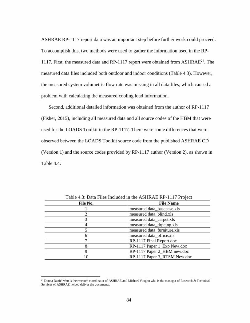
84
ASHRAE RP-1117 report data was an important step before further work could proceed.
To accomplish this, two methods were used to gather the information used in the RP-
1117. First, the measured data and RP-1117 report were obtained from ASHRAE24. The
measured data files included both outdoor and indoor conditions (Table 4.3). However,
the measured system volumetric flow rate was missing in all data files, which caused a
problem with calculating the measured cooling load information.
Second, additional detailed information was obtained from the author of RP-1117
(Fisher, 2015), including all measured data and all source codes of the HBM that were
used for the LOADS Toolkit in the RP-1117. There were some differences that were
observed between the LOADS Toolkit source code from the published ASHRAE CD
(Version 1) and the source codes provided by RP-1117 author (Version 2), as shown in
Table 4.4.
Table 4.3: Data Files Included in the ASHRAE RP-1117 Project
File No. File Name
1 measured data_basecase.xls
2 measured data_blind.xls
3 measured data_carpet.xls
4 measured data_drpclng.xls
5 measured data_furniture.xls
6 measured data_office.xls
7 RP-1117 Final Report.doc
8 RP-1117 Paper 1_Exp New.doc
9 RP-1117 Paper 2_HBM new.doc
10 RP-1117 Paper 3_RTSM New.doc
24 Donna Daniel who is the research coordinator of ASHRAE and Michael Vaughn who is the manager of Research & Technical Services of ASHRAE helped deliver the documents.

85
Table 4.4: HB LOADS Toolkit Source Code Comparisons No. Source Code Version 1 Source Code Version 2 Comments
1 N/A BlindEplus.f90
PUBLIC EplusBlind PRIVATE ManageOpticalCalculations
PRIVATE CalcFenestrationProperties
PRIVATE GetBlindData PRIVATE InitBlindData
PRIVATE AngOptProp
PRIVATE ProfileAngle PRIVATE CalcWindowBlindProperties
PRIVATE BlindOpticsDiffuse
PRIVATE BlindOpticsBeam PRIVATE ViewFac
PRIVATE InvertMatrix
PRIVATE LUDCMP
PRIVATE LUBKSB
PRIVATE DiffuseAverage
2 N/A BlindGlsim.f90
PUBLIC GlsimBlind
PRIVATE GetBlindData PRIVATE ProfileAngle
PRIVATE DirectTrans
PRIVATE DiffuseTrans PRIVATE AngOptProp
PRIVATE Interaction
PRIVATE DirectGlazing
PRIVATE DiffuseGlazing
PRIVATE DirReflDiff PRIVATE DirReflSpec
PRIVATE DiffRefl
3 N/A BlindParmelee.f90
PUBLIC ParmeleeBlind
PRIVATE GetBlindData PRIVATE AngOptProp
PRIVATE ProfileAngle
PRIVATE DirectDiffuseBlindCalc PRIVATE DirectSpecularBlindCalc
PRIVATE SkyDiffuseBlindCalc
PRIVATE GroundDiffuseBlindCalc PRIVATE ConfigurationFactor
PRIVATE CosIncidentAngle
PRIVATE Interaction
4 CTFMod.f90 CTFMod.f90
5 N/A DataConversions.f90 Conversion for Conduction Transfer Functions
6 EnvrnSurfTemperatureMod.f90 EnvrnSurfTemperatureMod.f90

86
Table 4.4 Continued No. Source Code Version 1 Source Code Version 2 Comments
7 ExteriorConvectionMod.f90 ExteriorConvectionMod.f90
8 ExteriorLWRadiationMod.f90 ExteriorLWRadiationMod.f90
9 N/A General.f90
PUBLIC SolveRegulaFalsi
PUBLIC POLYF
PUBLIC InterpSw
PUBLIC InterpBlind
PUBLIC InterpSlatAng
PUBLIC InterpProfAng PUBLIC InterpProfSlatAng
PUBLIC BlindBeamBeamTrans
PUBLIC POLY1F ! Not currently used in EnergyPlus (Dec 2001)
PUBLIC POLY2F ! Not currently used in
EnergyPlus (Dec 2001)
10 GroundTemperatureMod.f90 GroundTemperatureMod.f90
11 InfiltrationVentilationMod.f90 InfiltrationVentilationMod.f90
12 InputProcessor.f90 InputProcessor.f90
1). Add SUBROUTINE
ShowContinueError(Message,Unit1,Unit2)
2). Add SUBROUTINE
ShowContinueError(Message,OutUnit1,OutUnit2)
13 InteriorConvectionMod.f90 InteriorConvectionMod.f90 1). Add SUBROUTINE
CalculateHcInCeilingDiffuser
14 InternalGainsMod.f90 InternalGainsMod.f90
15 IRViewsToGroundAndSky.f90 IRViewsToGroundAndSky.f90
16 PsychrometricsMod.f90 PsychrometricsMod.f90
17 RadiativeGainsDistributionMod.f90 RadiativeGainsDistributionMod.f90 1). SUBROUTINE DetailedRadGainsDistribs
2). SUBROUTINE GetBeamRadDistribInput
18 ShadingMod.f90 ShadingMod.f90
19 SkyRadiationMod.f90 SkyRadiationMod.f90 1). SUBROUTINE MeasuredSkyModel
2). SUBROUTINE EPlusClearSkyModel
20 SkyTemperatureModelsMod.f90 SkyTemperatureModelsMod.f90 1).Add USE PsychrometricsMod, ONLY : SATPRESS
21 SolarPosition.f90 SolarPosition.f90
1).Add SUBROUTINE
EplusDeclinationAndTime
2).Add SUBROUTINE JulianDay
22 SolarViewsToGroundAndSky.f90 SolarViewsToGroundAndSky.f90 1).Add SUBROUTINE AnisoSkyViewFactors
23 SuccessiveSubstitutionSolution.f90 SuccessiveSubstitutionSolution_Baseline
Model.f90 1). Add SUBROUTINE GetWindInput
24 Toolkit.f90 Toolkit.f90
25 UtilityMod.f90 UtilityMod.f90
26 ViewFactorMod.f90 ViewFactorMod.f90
27 Windows.f90 Windows.f90
28 ZoneLWRadiationMod.f90 ZoneLWRadiationMod.f90
All source codes were loaded into the Eclipse FORTRAN compiler (The Elipse
Foundation, 2016), which was used to compile, link, and generate the executable file. In
this way, the input files for heavy-weight and light-weight building cases were run by
the two executable files that were compiled using two sets of source codes, which
allowed for the cooling load differences as shown in Figure 4.5 and Figure 4.8. Figure
4.5 and Figure 4.8 show the comparisons of cooling load calculated by the executable

87
files generated by compiling source code Versions 1 and 2 for heavy-weight and light-
weight building cases. The graphs clearly showed the results from source code version 2
were offset, when compared to Version 1. The largest offset was observed to be from
7:00 a.m. to 4:00 p.m., with an inverse offset from 4:00 p.m. to 5 p.m.
Using the source code (Version 1) contained in the ASHRAE LOADS Toolkit CD
failed to replicate the cooling load results in the ASHRAE RP-1117 report as shown in
Figure 4.6 and Figure 4.9. The graphs clearly showed the two results were not matching,
with an R2 equaling to 0.9668 and 0.9681 for heavy-weight and light-weight building
cases, respectively.
However, the source code (Version 2) successfully calculated the same cooling load
results as shown in Figure 4.7 and Figure 4.10, which showed the cooling load matched
with the published results in the ASHRAE RP-1117 report, with an R2 equal to 1.
Therefore, the published results performed by HBM are considered validated and ready
to be used in the further cooling load comparisons.
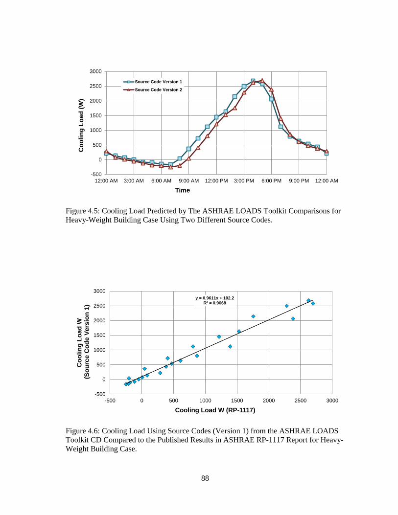
88
-500
0
500
1000
1500
2000
2500
3000
12:00 AM 3:00 AM 6:00 AM 9:00 AM 12:00 PM 3:00 PM 6:00 PM 9:00 PM 12:00 AM
Co
oli
ng
Lo
ad
(W
)
Time
Source Code Version 1
Source Code Version 2
Figure 4.5: Cooling Load Predicted by The ASHRAE LOADS Toolkit Comparisons for
Heavy-Weight Building Case Using Two Different Source Codes.
y = 0.9611x + 102.2R² = 0.9668
-500
0
500
1000
1500
2000
2500
3000
-500 0 500 1000 1500 2000 2500 3000
Co
oli
ng
Lo
ad
W(S
ou
rce
Co
de
Ve
rsio
n 1
)
Cooling Load W (RP-1117)
Figure 4.6: Cooling Load Using Source Codes (Version 1) from the ASHRAE LOADS
Toolkit CD Compared to the Published Results in ASHRAE RP-1117 Report for Heavy-
Weight Building Case.
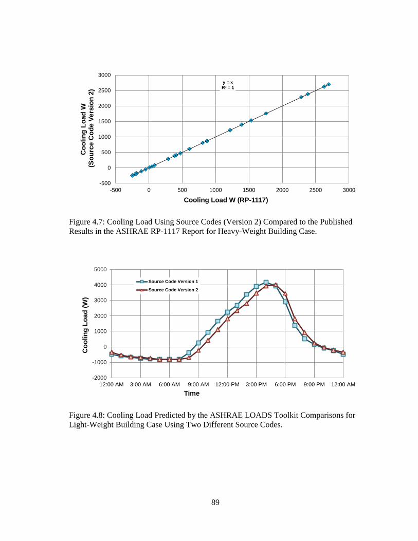
89
y = xR² = 1
-500
0
500
1000
1500
2000
2500
3000
-500 0 500 1000 1500 2000 2500 3000
Co
oli
ng
Lo
ad
W(S
ou
rce
Co
de
Ve
rsio
n 2
)
Cooling Load W (RP-1117)
Figure 4.7: Cooling Load Using Source Codes (Version 2) Compared to the Published
Results in the ASHRAE RP-1117 Report for Heavy-Weight Building Case.
-2000
-1000
0
1000
2000
3000
4000
5000
12:00 AM 3:00 AM 6:00 AM 9:00 AM 12:00 PM 3:00 PM 6:00 PM 9:00 PM 12:00 AM
Co
oli
ng
Lo
ad
(W
)
Time
Source Code Version 1
Source Code Version 2
Figure 4.8: Cooling Load Predicted by the ASHRAE LOADS Toolkit Comparisons for
Light-Weight Building Case Using Two Different Source Codes.
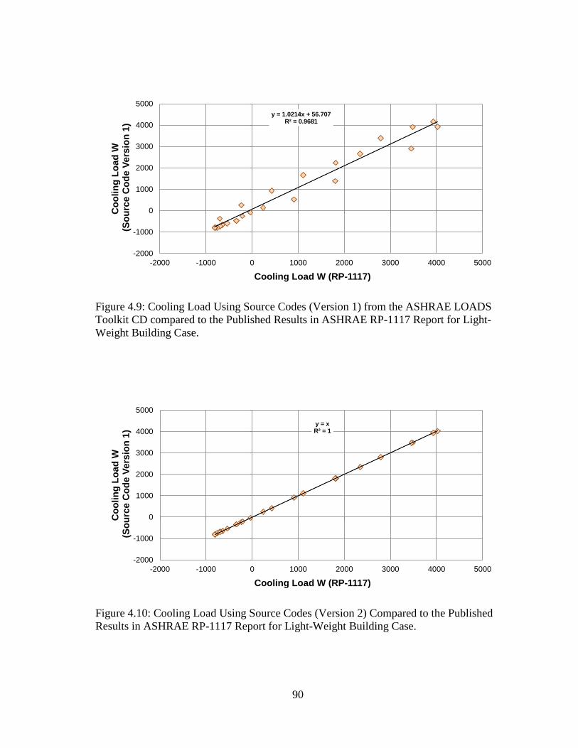
90
y = 1.0214x + 56.707R² = 0.9681
-2000
-1000
0
1000
2000
3000
4000
5000
-2000 -1000 0 1000 2000 3000 4000 5000
Co
oli
ng
Lo
ad
W(S
ou
rce
Co
de
Ve
rsio
n 1
)
Cooling Load W (RP-1117)
Figure 4.9: Cooling Load Using Source Codes (Version 1) from the ASHRAE LOADS
Toolkit CD compared to the Published Results in ASHRAE RP-1117 Report for Light-
Weight Building Case.
y = xR² = 1
-2000
-1000
0
1000
2000
3000
4000
5000
-2000 -1000 0 1000 2000 3000 4000 5000
Co
oli
ng
Lo
ad
W(S
ou
rce
Co
de
Ve
rsio
n 1
)
Cooling Load W (RP-1117)
Figure 4.10: Cooling Load Using Source Codes (Version 2) Compared to the Published
Results in ASHRAE RP-1117 Report for Light-Weight Building Case.
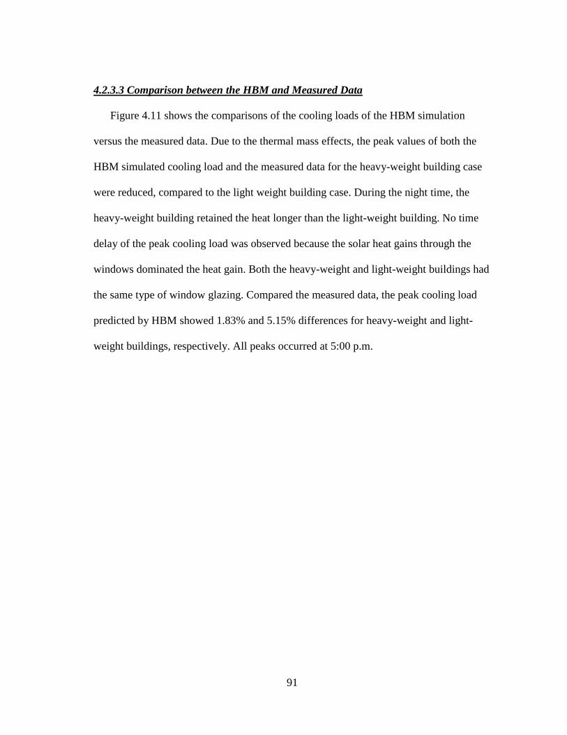
91
4.2.3.3 Comparison between the HBM and Measured Data
Figure 4.11 shows the comparisons of the cooling loads of the HBM simulation
versus the measured data. Due to the thermal mass effects, the peak values of both the
HBM simulated cooling load and the measured data for the heavy-weight building case
were reduced, compared to the light weight building case. During the night time, the
heavy-weight building retained the heat longer than the light-weight building. No time
delay of the peak cooling load was observed because the solar heat gains through the
windows dominated the heat gain. Both the heavy-weight and light-weight buildings had
the same type of window glazing. Compared the measured data, the peak cooling load
predicted by HBM showed 1.83% and 5.15% differences for heavy-weight and light-
weight buildings, respectively. All peaks occurred at 5:00 p.m.

92
-1500
0
1500
3000
4500
6000
7500
12:00 AM 3:00 AM 6:00 AM 9:00 AM 12:00 PM 3:00 PM 6:00 PM 9:00 PM 12:00 AM
(W)
Time
HBM-Heavy
HBM-Light
Measured Data-Heavy
Measured Data-Light
(a)
-1000
-500
0
500
1000
1500
2000
2500
3000
3500
4000
12:00 AM 3:00 AM 6:00 AM 9:00 AM 12:00 PM 3:00 PM 6:00 PM 9:00 PM 12:00 AM
(W)
Time
Heavy(HBM-Measured)
Light(HBM-Measured)
(b)(b)
0
5
10
15
20
25
30
35
0
100
200
300
400
500
600
700
800
900
1000
12:00 AM 3:00 AM 6:00 AM 9:00 AM 12:00 PM 3:00 PM 6:00 PM 9:00 PM 12:00 AM
Te
mp
era
ture
(C
)W
ind
Sp
ee
d (
m/s
)
So
lar
Ra
dia
tio
n (
W/m
2)
Time
Global Solar Radiation Tdb WS Tin-Heavy Tin-Light
(c) Figure 4.11: HBM versus Measured Data: (a) Cooling Load Comparisons between HBM
and Measured Data for Heavy-Weight and Light-Weight Buildings; (b) Cooling Load
Differences between HBM and Measured Data for Heavy-Weight and Light-Weight
Buildings; and (c) Weather Conditions for September 22nd 2001, Stillwater, OK.

93
4.2.4 Radiant Time Series Method
The Radiant Time Series Method (RTSM) can be applied using the ASHRAE
LOADS Toolkit (Pedersen et al., 2001) or the ASHRAE RTSM spreadsheet tool (Spitler,
2009), shown in Table 4.5. The 2009 ASHRAE RTSM spreadsheet tool was adopted in
this process to predict the cooling loads of the selected study cases. The RTSM
procedure is detailed in Appendix E.
The ASHRAE RTSM spreadsheet tool consists of several individual spreadsheets,
covering the calculations of solar, Conduction Time Series Factors (CTSFs), Radiant
Time Factors (RTFs), and contains an example of a whole-room application.
Table 4.5: Tools for RTSM Simulation
ASHRAE LOADS Toolkit ASHRAE RTSM Spreadsheet
File Names
-Source codes;
-in. idf;
-ToolkitTest.idd;
-Toolkit.err;
-RadiantTimeSeries.exe;
-audit.out;
-RTSoutput.put
-Weather stations;
- 7-1-solar.xls;
- 7-3_tabulated_CTSF.xls;
- 7-4_generate_CTSF.xls;
- 7-6 RTF_tabulated.xls;
- B-1_RTSM.xls;
- C-1_CTFSgen.xls;
- C-2_RTFgen.xls;
- D-1-solar.xls;
- Example 7.1 Compute CTSF.xls;
- Example 7.1 Conduction.xls;
- Example 7.2 Window.xls;
- Example 7.3 RTF generation.xls;
- Example 7.4 ClgLoad from Heat
Gain.xls;
- Example 8.1 Compute CTSF.xls;
- Example 8.1 Compute RTF.xls;
- Example 8.1 Conduction HG.xls;
- Example 8.1 solar.xls;

94
4.2.4.1 Weather Data File Review
Since the default weather information that is provided with RTSM spreadsheet tool
does not include the Stillwater, OK, weather data additional was added manually. The
input information consisted of latitude, longitude, elevation, monthly design dry bulb
and mean coincident wet bulb temperatures, and mean daily temperature range.
While reading through the weather condition data published in 2009 ASHRAE
Handbook of Fundamentals, it was noticed that at the bottom of the data sheet, a section
named “clear-sky solar irradiance” was added, compared to previous weather data. This
yielded the values of beam and diffuse optical depth and default radiation that are
needed in the 2009 ASHRAE clear- sky model, which is detailed in Appendix B.
For the actual design process, the design conditions needed to be used to perform the
peak load calculations. By using the peak design temperature and daily range provided
by the weather condition files, the ASHRAE hourly outside dry bulb temperature can be
determined by (ASHRAE, 2005),
peak ht t f DR (4.11)
where,
peakt : peak design dry bulb temperature, C;
hf : daily temperature range fraction, dimensionless, see Table 4.6;
DR : daily range of dry bulb temperature, C;

95
Table 4.6: Daily Temperature Range Fraction (Adapted from ASHRAE, 2005)
Time, h f Time, h f Time, h f 1 0.87 9 0.71 17 0.10
2 0.92 10 0.56 18 0.21
3 0.96 11 0.39 19 0.34
4 0.99 12 0.23 20 0.47
5 1.00 13 0.11 21 0.58
6 0.98 14 0.03 22 0.68
7 0.93 15 0.00 23 0.76
8 0.84 16 0.03 24 0.82
An equation that represents the ASHRAE fraction data was presented (Spitler, 2009).
This equation was also adopted in RTSM spreadsheet tool, which is given by,
11
0
2 2[ cos( ) sin( )]
24 24peak i i
i
i it t DR a b
(4.12)
where,
ia , ib : equation-fit coefficients, dimensionless, see Table 4.7;
: the apparent solar time in decimal form, dimensionless;
Table 4.7: Equation-Fit Coefficients (Adapted from Spitler, 2009)
i ia
ib
0 0.5629 0.0000
1 0.2932 0.3848
2 -0.0348 -0.0835
3 -0.0006 -0.0006
4 -0.0017 0.0000
5 0.0013 -0.0004
6 0.0000 -0.0008
7 0.0004 -0.0010
8 -0.0017 0.0000
9 0.0006 -0.0006
10 -0.0002 0.0002
11 0.0001 0.0003
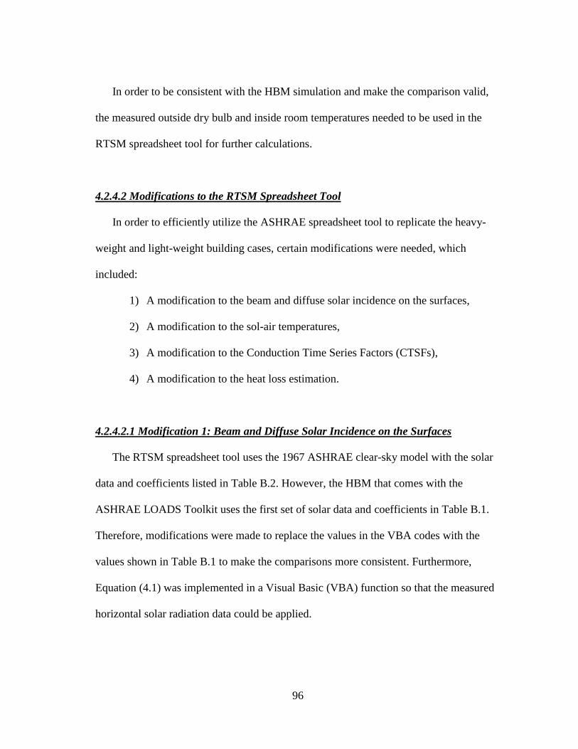
96
In order to be consistent with the HBM simulation and make the comparison valid,
the measured outside dry bulb and inside room temperatures needed to be used in the
RTSM spreadsheet tool for further calculations.
4.2.4.2 Modifications to the RTSM Spreadsheet Tool
In order to efficiently utilize the ASHRAE spreadsheet tool to replicate the heavy-
weight and light-weight building cases, certain modifications were needed, which
included:
1) A modification to the beam and diffuse solar incidence on the surfaces,
2) A modification to the sol-air temperatures,
3) A modification to the Conduction Time Series Factors (CTSFs),
4) A modification to the heat loss estimation.
4.2.4.2.1 Modification 1: Beam and Diffuse Solar Incidence on the Surfaces
The RTSM spreadsheet tool uses the 1967 ASHRAE clear-sky model with the solar
data and coefficients listed in Table B.2. However, the HBM that comes with the
ASHRAE LOADS Toolkit uses the first set of solar data and coefficients in Table B.1.
Therefore, modifications were made to replace the values in the VBA codes with the
values shown in Table B.1 to make the comparisons more consistent. Furthermore,
Equation (4.1) was implemented in a Visual Basic (VBA) function so that the measured
horizontal solar radiation data could be applied.
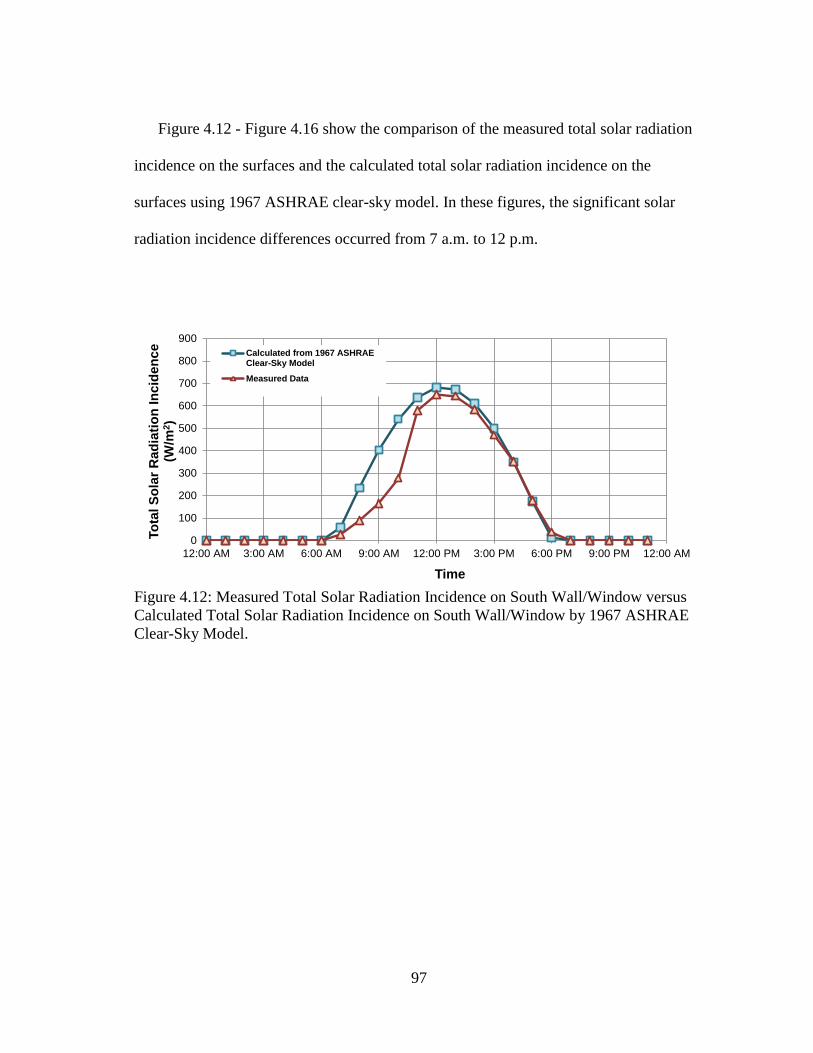
97
Figure 4.12 - Figure 4.16 show the comparison of the measured total solar radiation
incidence on the surfaces and the calculated total solar radiation incidence on the
surfaces using 1967 ASHRAE clear-sky model. In these figures, the significant solar
radiation incidence differences occurred from 7 a.m. to 12 p.m.
0
100
200
300
400
500
600
700
800
900
12:00 AM 3:00 AM 6:00 AM 9:00 AM 12:00 PM 3:00 PM 6:00 PM 9:00 PM 12:00 AM
To
tal S
ola
r R
ad
iati
on
In
cid
en
ce
(W
/m2)
Time
Calculated from 1967 ASHRAEClear-Sky Model
Measured Data
Figure 4.12: Measured Total Solar Radiation Incidence on South Wall/Window versus
Calculated Total Solar Radiation Incidence on South Wall/Window by 1967 ASHRAE
Clear-Sky Model.
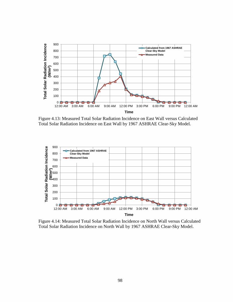
98
0
100
200
300
400
500
600
700
800
900
12:00 AM 3:00 AM 6:00 AM 9:00 AM 12:00 PM 3:00 PM 6:00 PM 9:00 PM 12:00 AM
To
tal S
ola
r R
ad
iati
on
In
cid
en
ce
(W
/m2)
Time
Calculated from 1967 ASHRAEClear-Sky Model
Measured Data
Figure 4.13: Measured Total Solar Radiation Incidence on East Wall versus Calculated
Total Solar Radiation Incidence on East Wall by 1967 ASHRAE Clear-Sky Model.
0
100
200
300
400
500
600
700
800
900
12:00 AM 3:00 AM 6:00 AM 9:00 AM 12:00 PM 3:00 PM 6:00 PM 9:00 PM 12:00 AM
To
tal S
ola
r R
ad
iati
on
In
cid
en
ce
(W
/m2)
Time
Calculated from 1967 ASHRAEClear-Sky Model
Measured Data
Figure 4.14: Measured Total Solar Radiation Incidence on North Wall versus Calculated
Total Solar Radiation Incidence on North Wall by 1967 ASHRAE Clear-Sky Model.

99
0
100
200
300
400
500
600
700
800
900
12:00 AM 3:00 AM 6:00 AM 9:00 AM 12:00 PM 3:00 PM 6:00 PM 9:00 PM 12:00 AM
To
tal S
ola
r R
ad
iati
on
In
cid
en
ce
(W
/m2)
Time
Calculated from 1967 ASHRAEClear-Sky Model
Measured Data
Figure 4.15: Measured Total Solar Radiation Incidence on West Wall/Window versus
Calculated Total Solar Radiation Incidence on West Wall/Window by 1967 ASHRAE
Clear-Sky Model.
0
100
200
300
400
500
600
700
800
900
12:00 AM 3:00 AM 6:00 AM 9:00 AM 12:00 PM 3:00 PM 6:00 PM 9:00 PM 12:00 AM
To
tal S
ola
r R
ad
iati
on
In
cid
en
ce
(W
/m2)
Time
Calculated from 1967 ASHRAEClear-Sky Model
Measured Data
Figure 4.16: Measured Total Solar Radiation Incidence on Roof versus Calculated Total
Solar Radiation Incidence on Roof by 1967 ASHRAE Clear-Sky Model.
100
4.2.4.2.2 Modification 2: Sol-Air Temperatures
For the exterior surfaces with boundary condition to the outside, sol-air temperature
relies on the total solar radiation incidence on the specific surface as well as the outside
dry bulb temperature. Since the measured data was used, the sol-air temperatures were
recalculated for each surface.
4.2.4.2.3 Modification 3: Conduction Time Series Factors (CTSFs)
The RTSM load calculation procedures are listed in Appendix E. In the conduction
heat gain calculations for exterior surfaces, two factors are introduced: Periodic
Response Factors (PRFs) and Conduction Time Series Factors (CTSFs). The difference
between the two is that the CTSFs are dimensionless factors and can be determined by
the PRFs divided by the U factor. In the ASHRAE RP-1117 report, the PRFs were input
by the users, while the RTSM spreadsheet tool calculates the CTSFs from the user inputs
for the construction material layers. If the material layers are the same, only one set of
the response factors can be obtained. However, some discrepancies were observed
between the calculated CTSFs by RTSM spreadsheet tool and the ones used in the RP-
1117 report.
First, though the wall materials were the same, the PRFs input values were different.
Figure 4.17 and Figure 4.19 showed the PRFs differences for heavy-weight and light-
weight building cases. Figure 4.18 and Figure 4.20 showed the calculated CTSFs
comparisons between the ASHRAE RP-1117 report inputs and the ones calculated by
the RTSM spreadsheet tool. In the comparison, it can be observed that the hourly CTSFs

101
pattern and values were different. Therefore, in the current study, the inputs from RP-
1117 report were adopted to perform the comparisons.
0.00
0.02
0.04
0.06
0.08
0.10
0.12
0.14
0 1 2 3 4 5 6 7 8 9 10 11 12 13 14 15 16 17 18 19 20 21 22 23
PR
Fs
(W/m
2-K
)
Time
South Wall
East Wall
North Wall
West Wall
Figure 4.17: Wall PRFs Inputs by ASHRAE RP-1117 Report for Heavy-Weight
Building.
0.00
0.02
0.04
0.06
0.08
0.10
0.12
0.14
0 1 2 3 4 5 6 7 8 9 10 11 12 13 14 15 16 17 18 19 20 21 22 23
CT
SF
s
Time
South Wall(RP-1117)
East Wall(RP-1117)
North Wall(RP-1117)
West Wall(RP-1117)
Roof(RP-1117)
All Walls by RTSM Spreadsheet
Roof by RTSM Spreadsheet Tool
Figure 4.18: Calculated CTSFs Comparisons between the ASHRAE RP-1117 Report
Inputs and by RTSM Spreadsheet Tool for Heavy-Weight Building.
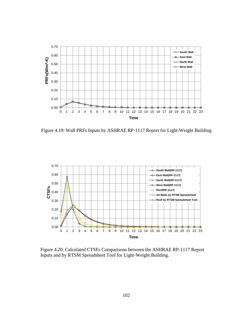
102
0.00
0.10
0.20
0.30
0.40
0.50
0.60
0.70
0 1 2 3 4 5 6 7 8 9 10 11 12 13 14 15 16 17 18 19 20 21 22 23
PR
Fs
(W/m
2-K
)
Time
South Wall
East Wall
North Wall
West Wall
Figure 4.19: Wall PRFs Inputs by ASHRAE RP-1117 Report for Light-Weight Building
0.00
0.10
0.20
0.30
0.40
0.50
0.60
0.70
0 1 2 3 4 5 6 7 8 9 10 11 12 13 14 15 16 17 18 19 20 21 22 23
CT
SF
s
Time
South Wall(RP-1117)
East Wall(RP-1117)
North Wall(RP-1117)
West Wall(RP-1117)
Roof(RP-1117)
All Walls by RTSM Spreadsheet
Roof by RTSM Spreadsheet Tool
Figure 4.20: Calculated CTSFs Comparisons between the ASHRAE RP-1117 Report
Inputs and by RTSM Spreadsheet Tool for Light-Weight Building.

103
4.2.4.2.4 Modification 4: Heat Loss Estimation
The RTSM tends to over-predict a cooling load when performing the space cooling
load calculations. This is due to the assumption of an adiabatic boundary condition when
applying the heat balance to the zone model and in generating the Radiant Time Factors
(RTFs) (Fisher and Spitler, 2002; Nigusse, 2007; Rees et al., 2000; Rees et al., 1998). In
the RTSM, once all types of heat gains enter the space, no heat loss is allowed in the
calculation procedure (Fisher and Spitler, 2002).
In contrast, the ASHRAE RP-1117 report proposed a new methodology to account
for the radiant heat loss out of the zone (Fisher and Spitler, 2002), and Nigusse derived
four new approaches to implement the heat loss calculations by introducing the interior
sol-air temperature concept (Nigusse, 2007; Nigusse and Spitler, 2010). However, it was
determined that the RTSM spreadsheet tool has yet to implement those heat loss
calculation procedures. Therefore, users need to perform the heat loss calculations and
subtract it from the total radiant heat gains before applying the RTFs. Using the
methodology shown in ASHRAE RP-1117 report. the heat loss calculations were
performed in order to simulate the heavy-weight and light-weight building cases.
#
, , , , , ,
0
( )windows
SW loss floor t floor beam diffuse k t k
k
Q s Q Q s
(4.13)
where,
floors : solar fraction of the floor, dimensionless;
,t floor : floor solar reflectance, dimensionless;
,beamQ : beam solar radiation that enters the space, W;

104
,diffuseQ : diffuse solar radiation that enters the space, W;
ks : solar fraction of the window, dimensionless;
,t k : window transmittance, dimensionless.
4.2.4.3 Comparison between the RTSM and Measured Data
Figure 4.21 shows the comparisons of peak cooling loads using the RTSM procedure
versus the measured data. In the comparison, similar observations to the HBM
simulation were found for the thermal mass influences. Compared to the measured data,
the RTSM over-predicted the cooling load for both the heavy-weight and light-weight
building cases, which were 68.32 % and 57.83% differences, respectively. The estimated
peak did occur at 5:00 p.m., which was the same time as the HBM and the measured
data for both cases. The cooling load difference between the RTSM and the measured
data showed large variations starting from 12:00 p.m. to 5:00 p.m. The light-weight
building case tended to have an even larger difference compared to the heavy-weight
building case.
There were two reasons mentioned in ASHRAE RP-1117 report for the RTSM over-
predicting the space cooling load compared to the HBM. One is the original assumptions
used in the RTSM, which converts all types of heat gains to cooling load, using Radiant
Time Factors (RTFs). These are generated by applying the HBM to an adiabatic zone.
This means the heat can enter into the space but cannot exit. Unfortunately, with a large
amount of glazing on south and west walls, a large amount of solar heat gain enters the
room and heats up the indoor temperature immediately, which then causes a rise in

105
inside surface temperatures of the exterior surfaces. Sometimes this inside surface
temperature can be larger than the outside temperature. Therefore, a heat loss out of the
space can be occurring. Unfortunately, the calculated RP-1117 RTFs cannot reflect this
situation. Second, there is a difference in conduction calculations. Specifically, the HBM
utilizes a surface temperature gradient to perform the calculation, while the RTSM uses
the air temperature difference. Even with the corrections of heat loss calculations that
were recommended from ASHRAE RP-1117 report, the over-predicting issue still
existed. Finally, the RTSM results that were reproduced in this study still did not match
the published values in the ASHRAE RP-1117 report. The reasons for this remain
unknown.
Finally, considering the fact that the modifications were added for the outside
calculations of RTFs, this may not solve the root of the issue. Therefore, in the future it
is suggested that the RTFs be recalculated by applying proper boundary conditions.

106
-1500
0
1500
3000
4500
6000
7500
12:00 AM 3:00 AM 6:00 AM 9:00 AM 12:00 PM 3:00 PM 6:00 PM 9:00 PM 12:00 AM
(W)
Time
RTSM-Heavy
RTSM-Light
Measured Data-Heavy
Measured Data-Light
-1000
-500
0
500
1000
1500
2000
2500
3000
3500
4000
12:00 AM 3:00 AM 6:00 AM 9:00 AM 12:00 PM 3:00 PM 6:00 PM 9:00 PM 12:00 AM
(W)
Time
Heavy(RTSM-Measured)
Light(RTSM-Measured)
(b)(b)
0
5
10
15
20
25
30
35
0
100
200
300
400
500
600
700
800
900
1000
12:00 AM 3:00 AM 6:00 AM 9:00 AM 12:00 PM 3:00 PM 6:00 PM 9:00 PM 12:00 AM
Te
mp
era
ture
(C
)W
ind
Sp
ee
d (
m/s
)
So
lar
Ra
dia
tio
n (
W/m
2)
Time
Global Solar Radiation Tdb WS Tin-Heavy Tin-Light
(c)
(a)
Figure 4.21: RTSM versus Measured Data: (a) Cooling Load Comparisons between
RTSM and Measured Data for Heavy-Weight and Light-Weight Buildings; (b) Cooling
Load Differences between RTSM and Measured Data for Heavy-Weight and Light-
Weight Buildings; and (c) Weather Conditions for September 22nd 2001, Stillwater, OK.

107
4.2.5 Transfer Function Method
In the same fashion as the RTSM, the TFM is also a two-step calculation method,
involving Conduction Transfer Functions (CTFs) and Room Transfer Functions (RTFs,
also called Weighting Factors) to determine the peak cooling load. Appendix F details
the TFM cooling load calculation procedure. Compared to the RTSM, the calculations of
wall/roof conduction heat gains and cooling load in the TFM are varied. The fenestration
heat gain is calculated using Shading Coefficients (SC) and the published DSA Glass
coefficients according to the latest published TFM procedure (ASHRAE, 1997). Starting
from 2001 ASHRAE Handbook of Fundamentals, the TFM was eliminated from the
handbook and replaced with the HBM and the RTSM cooling load calculation methods.
As the RTSM was further developed, the fenestration model was updated to use angular
Solar Heat Gain Coefficients (SHGC) instead of the older, less accurate SC method. The
two fenestration model comparisons are shown in Appendix C. All other heat gain
calculations remained the same including the window conduction heat gains, internal
heat gains, and infiltration heat gains.
The following are the limitations of the TFM, which were observed from the current
study:
Construction layers’ thermal properties and code numbers are pre-defined. The
TFM relies on tables of pre-defined material layers. Therefore, the users who apply the
TFM must choose the proper code number according to the TFM tables, which uses the
published values in 1997 ASHRAE Handbook of Fundamentals (ASHRAE, 1997).
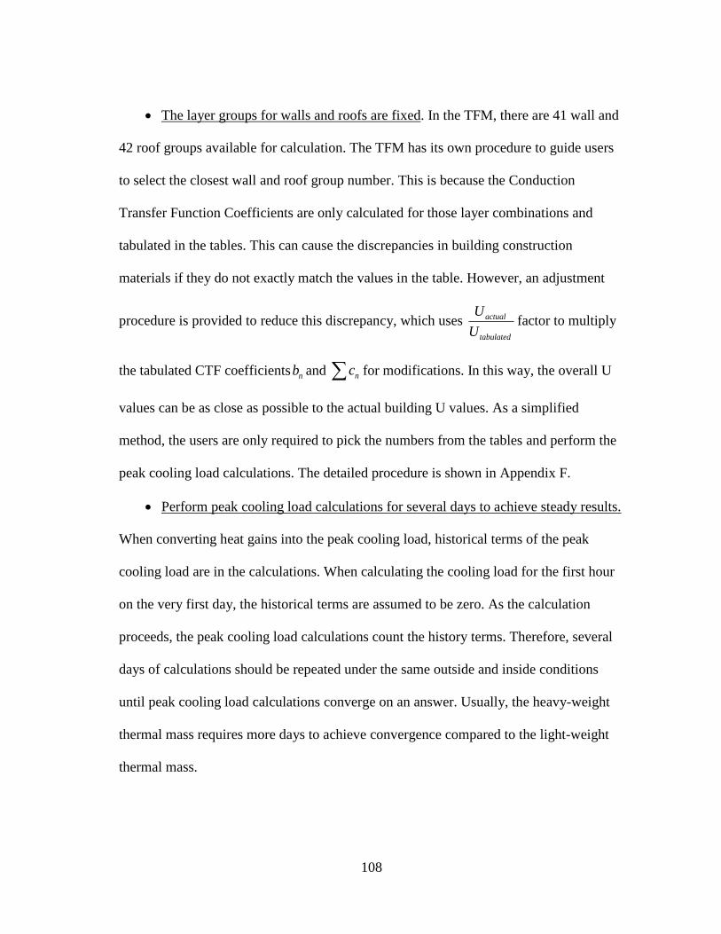
108
The layer groups for walls and roofs are fixed. In the TFM, there are 41 wall and
42 roof groups available for calculation. The TFM has its own procedure to guide users
to select the closest wall and roof group number. This is because the Conduction
Transfer Function Coefficients are only calculated for those layer combinations and
tabulated in the tables. This can cause the discrepancies in building construction
materials if they do not exactly match the values in the table. However, an adjustment
procedure is provided to reduce this discrepancy, which uses actual
tabulated
U
Ufactor to multiply
the tabulated CTF coefficients nb and nc for modifications. In this way, the overall U
values can be as close as possible to the actual building U values. As a simplified
method, the users are only required to pick the numbers from the tables and perform the
peak cooling load calculations. The detailed procedure is shown in Appendix F.
Perform peak cooling load calculations for several days to achieve steady results.
When converting heat gains into the peak cooling load, historical terms of the peak
cooling load are in the calculations. When calculating the cooling load for the first hour
on the very first day, the historical terms are assumed to be zero. As the calculation
proceeds, the peak cooling load calculations count the history terms. Therefore, several
days of calculations should be repeated under the same outside and inside conditions
until peak cooling load calculations converge on an answer. Usually, the heavy-weight
thermal mass requires more days to achieve convergence compared to the light-weight
thermal mass.

109
Finally, in order to perform the proper comparisons, the fenestration model that
contains the angular SHGC was adopted in the TFM procedure since this represents the
most recent fenestration model published in the ASHRAE Handbook of Fundamentals
(ASHRAE, 2013a).
4.2.5.1 Conduction Transfer Function Coefficients
Following the procedure stated in Appendix F, the proper group numbers for the
walls and roofs were selected for both the heavy-weight and light-weight building cases.
Table 4.8 lists the associated parameters that were required for the group selection.
Table 4.9 shows both the original tabulated Conduction Transfer Function
coefficients and the adjusted ones, given by the group number. Figure 4.22 and Figure
4.23 indicate that bn is associated with the peak cooling load profile and dn is the fading
pulse that is related to the historical terms.
During the peak load design process, it was observed that heavy-weight building
case needed nine days to achieve convergence and the light-weight building case needed
only four days, by applying the same boundary conditions for every day.
Table 4.8: Group Selections of Heavy-Weight and Light-Weight Buildings
Heavy-Weight Building Light-Weight Building
Wall Roof Wall Roof
Principal Material C18 C14 B7 B7
Secondary Material A2 - A1 -
Mass Location Mass in Mass in Mass integral Mass integral
Group No. 17 9 4 2

110
Table 4.9: Wall and Roof Conduction Transfer Function Coefficients of Heavy-Weight
and Light-Weight Buildings
Heavy-Weight Building Light-Weight Building
Wall Roof Wall Roof
Tabulated Values
b0 0.00000 0.00000 0.00006 0.00316
b1 0.00003 0.00139 0.00613 0.06827
b2 0.00076 0.01234 0.02181 0.07278
b3 0.00248 0.01424 0.01063 0.00814
b4 0.00170 0.00315 0.00076 0.00007
b5 0.00029 0.00013 0.00000 0.00000
b6 0.00010 0.00000 0.00000 0.00000
d0 1.00000 1.00000 1.00000 1.00000
d1 -2.00875 -1.40605 -1.37579 -0.60064
d2 1.37120 0.58814 0.61544 0.08602
d3 -0.37897 -0.09034 -0.09389 -0.00135
d4 0.03962 0.00444 0.00221 0.00000
d5 -0.00165 -0.00006 0.00000 0.00000
d6 0.00002 0.00000 0.00000 0.00000
Adjusted Values
b0 0.00000 0.00000 0.00006 0.00429
b1 0.00011 0.00147 0.00651 0.09272
b2 0.00278 0.01308 0.02316 0.09885
b3 0.00906 0.01509 0.01129 0.01106
b4 0.00621 0.00334 0.00081 0.00010
b5 0.00106 0.00014 0.00000 0.00000
b6 0.00037 0.00000 0.00000 0.00000
d0 1.00000 1.00000 1.00000 1.00000
d1 -2.00875 -1.40605 -1.37579 -0.60064
d2 1.37120 0.58814 0.61544 0.08602
d3 -0.37897 -0.09034 -0.09389 -0.00135
d4 0.03962 0.00444 0.00221 0.00000
d5 -0.00165 -0.00006 0.00000 0.00000
d6 0.00002 0.00000 0.00000 0.00000
∑cn=∑bn 0.01958 0.03311 0.04182 0.20701
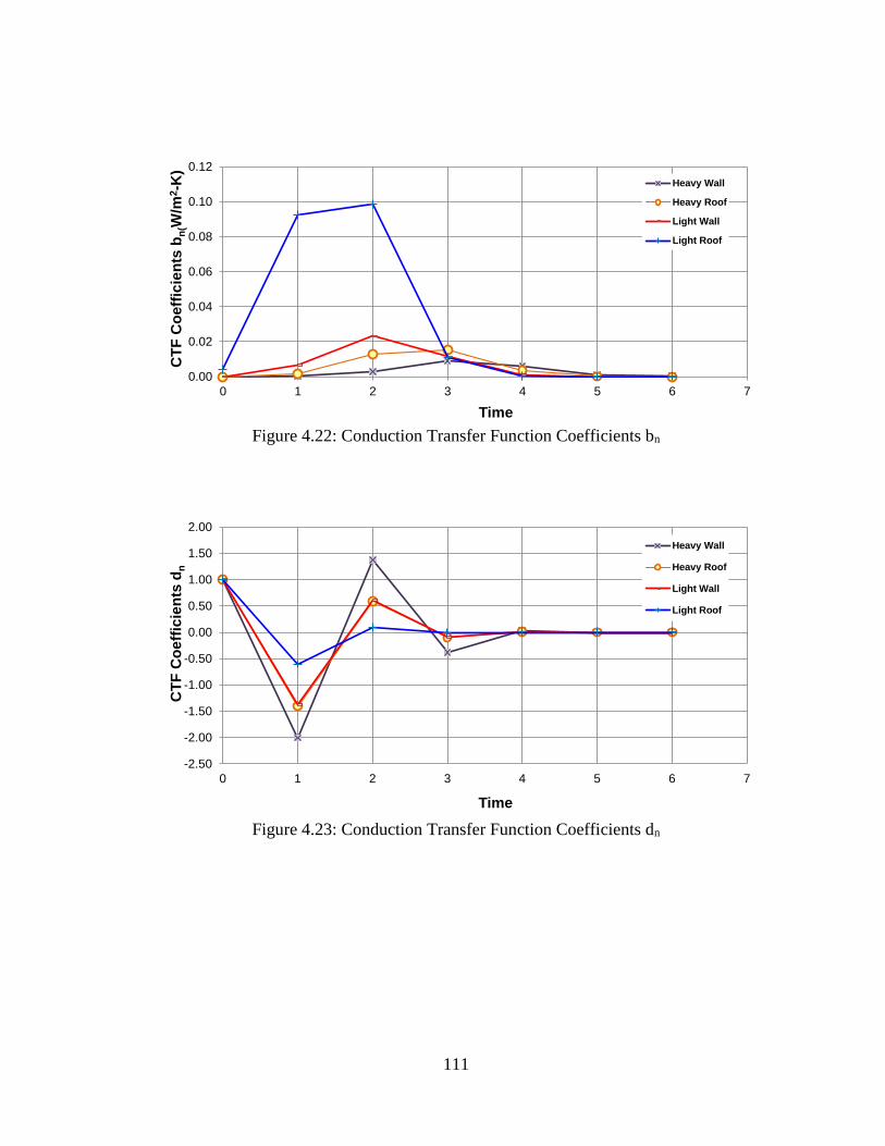
111
0.00
0.02
0.04
0.06
0.08
0.10
0.12
0 1 2 3 4 5 6 7
CT
F C
oe
ffic
ien
ts b
n(W
/m2-K
)
Time
Heavy Wall
Heavy Roof
Light Wall
Light Roof
Figure 4.22: Conduction Transfer Function Coefficients bn
-2.50
-2.00
-1.50
-1.00
-0.50
0.00
0.50
1.00
1.50
2.00
0 1 2 3 4 5 6 7
CT
F C
oe
ffic
ien
ts d
n
Time
Heavy Wall
Heavy Roof
Light Wall
Light Roof
Figure 4.23: Conduction Transfer Function Coefficients dn
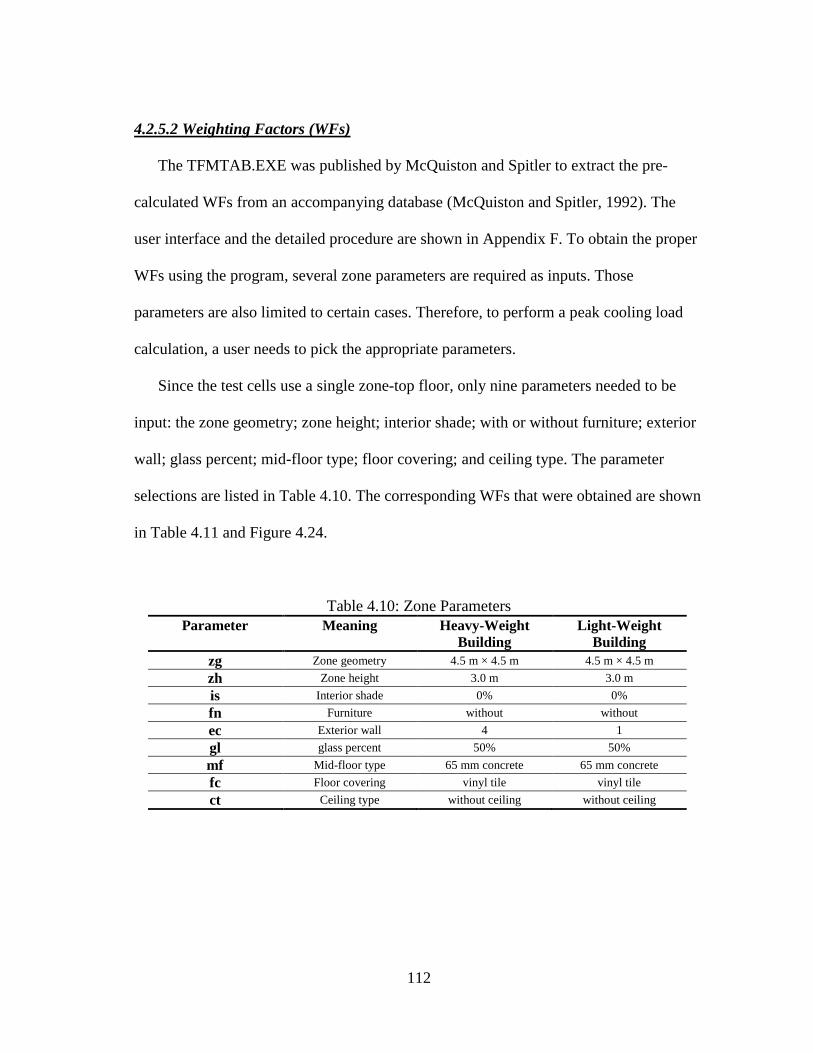
112
4.2.5.2 Weighting Factors (WFs)
The TFMTAB.EXE was published by McQuiston and Spitler to extract the pre-
calculated WFs from an accompanying database (McQuiston and Spitler, 1992). The
user interface and the detailed procedure are shown in Appendix F. To obtain the proper
WFs using the program, several zone parameters are required as inputs. Those
parameters are also limited to certain cases. Therefore, to perform a peak cooling load
calculation, a user needs to pick the appropriate parameters.
Since the test cells use a single zone-top floor, only nine parameters needed to be
input: the zone geometry; zone height; interior shade; with or without furniture; exterior
wall; glass percent; mid-floor type; floor covering; and ceiling type. The parameter
selections are listed in Table 4.10. The corresponding WFs that were obtained are shown
in Table 4.11 and Figure 4.24.
Table 4.10: Zone Parameters
Parameter Meaning Heavy-Weight
Building
Light-Weight
Building
zg Zone geometry 4.5 m × 4.5 m 4.5 m × 4.5 m
zh Zone height 3.0 m 3.0 m
is Interior shade 0% 0%
fn Furniture without without
ec Exterior wall 4 1
gl glass percent 50% 50%
mf Mid-floor type 65 mm concrete 65 mm concrete
fc Floor covering vinyl tile vinyl tile
ct Ceiling type without ceiling without ceiling
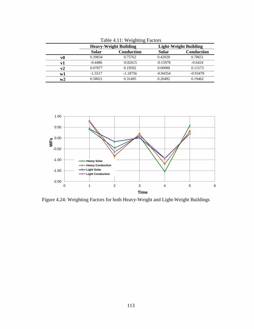
113
Table 4.11: Weighting Factors
Heavy-Weight Building Light-Weight Building
Solar Conduction Solar Conduction
v0 0.39834 0.75762 0.42028 0.78651
v1 -0.4486 -0.82615 -0.15978 -0.6424
v2 0.07877 0.19592 0.00088 0.11573
w1 -1.5517 -1.18756 -0.94354 -0.93478
w2 0.58021 0.31495 0.20492 0.19462
-2.00
-1.50
-1.00
-0.50
0.00
0.50
1.00
0 1 2 3 4 5 6
WF
s
Time
Heavy Solar
Heavy Conduction
Light Solar
Light Conduction
Figure 4.24: Weighting Factors for both Heavy-Weight and Light-Weight Buildings
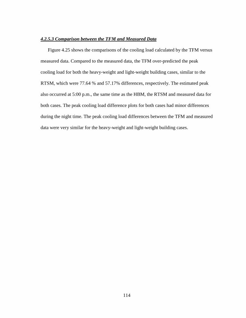
114
4.2.5.3 Comparison between the TFM and Measured Data
Figure 4.25 shows the comparisons of the cooling load calculated by the TFM versus
measured data. Compared to the measured data, the TFM over-predicted the peak
cooling load for both the heavy-weight and light-weight building cases, similar to the
RTSM, which were 77.64 % and 57.17% differences, respectively. The estimated peak
also occurred at 5:00 p.m., the same time as the HBM, the RTSM and measured data for
both cases. The peak cooling load difference plots for both cases had minor differences
during the night time. The peak cooling load differences between the TFM and measured
data were very similar for the heavy-weight and light-weight building cases.
115
-1500
0
1500
3000
4500
6000
7500
12:00 AM 3:00 AM 6:00 AM 9:00 AM 12:00 PM 3:00 PM 6:00 PM 9:00 PM 12:00 AM
(W)
Time
TFM-Heavy
TFM-Light
Measured Data-Heavy
Measured Data-Light
(a)
-1000
-500
0
500
1000
1500
2000
2500
3000
3500
4000
12:00 AM 3:00 AM 6:00 AM 9:00 AM 12:00 PM 3:00 PM 6:00 PM 9:00 PM 12:00 AM
(W)
Time
Heavy(TFM-Measured)
Light(TFM-Measured)
(b)(b)
0
5
10
15
20
25
30
35
0
100
200
300
400
500
600
700
800
900
1000
12:00 AM 3:00 AM 6:00 AM 9:00 AM 12:00 PM 3:00 PM 6:00 PM 9:00 PM 12:00 AM
Te
mp
era
ture
(C
)W
ind
Sp
ee
d (
m/s
)
So
lar
Ra
dia
tio
n (
W/m
2)
Time
Global Solar Radiation Tdb WS Tin-Heavy Tin-Light
(c)
Figure 4.25: TFM versus Measured Data: (a) Cooling Load Comparisons between TFM
and Measured Data for Heavy-Weight and Light-Weight Buildings; (b) Cooling Load
Differences between TFM and Measured Data for Heavy-Weight and Light-Weight
Buildings; and (c) Weather Conditions for September 22nd 2001, Stillwater, OK.
116
4.2.6 Total Equivalent Temperature Difference/Time Averaging Method (TETD/TA)
Among all the simplified methods, the TETD/TA Method was first introduced in the
ASHRAE Handbook of Fundamentals in 1967 (ASHRAE, 1967), coming from the ETD
tables by James P. Stewart in 1948. Appendix G details the TETD/TA methodology. In
the TETD/TA Method, the conduction heat gains through walls and roofs depend on
TETD multiplied by the UA. Hourly and averaged sol-air temperatures are used in the
TETD calculation. In addition, the thermal mass effects are calculated in TETD factors
by applying the proper decrement factors and time lags that can be found in the
published ASHRAE tables by defining specific walls/roofs group numbers, which
includes a total of 41 wall and 42 roof types to choose from. The solar heat gains
through fenestration are calculated by using Shading Coefficient (SC) according to the
most recent updates for TETD/TA Method (ASHRAE, 1997). Starting in 2001,
ASHRAE stopped publishing TETD/TA Method, retaining only the HBM and the
RTSM in the Handbook. As the RTSM developed, the fenestration solar heat gain
calculation model was updated using the angular SHGC. Additional information about
the comparison of the two models is contained in Appendix C. The differences between
TETD/TA and RTSM are the factors used for calculating the exterior surface conduction
heat gains and the method to convert all heat gains into the peak cooling load. Therefore,
the fenestration heat gain calculation can be updated for the peak cooling load
calculation method comparison process. The peak cooling load is finalized by applying
the Time Averaging (TA) process. Unfortunately, this requires a subjective decision to
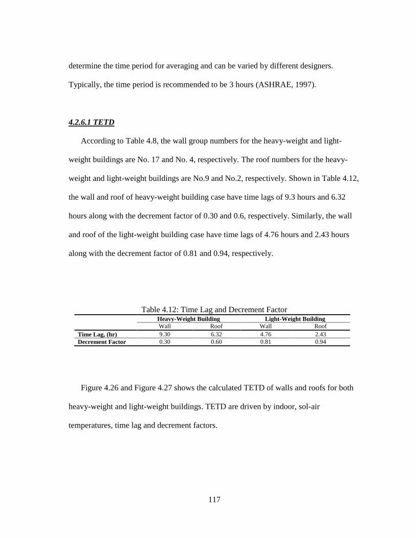
117
determine the time period for averaging and can be varied by different designers.
Typically, the time period is recommended to be 3 hours (ASHRAE, 1997).
4.2.6.1 TETD
According to Table 4.8, the wall group numbers for the heavy-weight and light-
weight buildings are No. 17 and No. 4, respectively. The roof numbers for the heavy-
weight and light-weight buildings are No.9 and No.2, respectively. Shown in Table 4.12,
the wall and roof of heavy-weight building case have time lags of 9.3 hours and 6.32
hours along with the decrement factor of 0.30 and 0.6, respectively. Similarly, the wall
and roof of the light-weight building case have time lags of 4.76 hours and 2.43 hours
along with the decrement factor of 0.81 and 0.94, respectively.
Table 4.12: Time Lag and Decrement Factor Heavy-Weight Building Light-Weight Building
Wall Roof Wall Roof
Time Lag, (hr) 9.30 6.32 4.76 2.43
Decrement Factor 0.30 0.60 0.81 0.94
Figure 4.26 and Figure 4.27 shows the calculated TETD of walls and roofs for both
heavy-weight and light-weight buildings. TETD are driven by indoor, sol-air
temperatures, time lag and decrement factors.
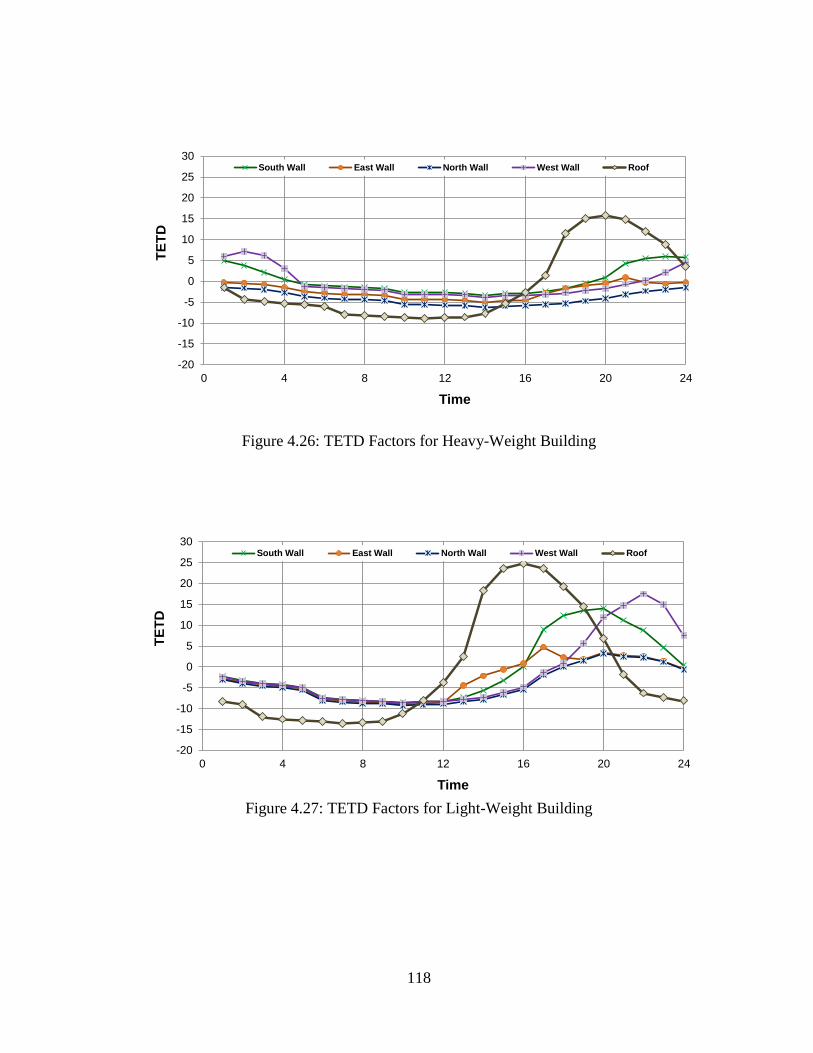
118
-20
-15
-10
-5
0
5
10
15
20
25
30
0 4 8 12 16 20 24
TE
TD
Time
South Wall East Wall North Wall West Wall Roof
Figure 4.26: TETD Factors for Heavy-Weight Building
-20
-15
-10
-5
0
5
10
15
20
25
30
0 4 8 12 16 20 24
TE
TD
Time
South Wall East Wall North Wall West Wall Roof
Figure 4.27: TETD Factors for Light-Weight Building
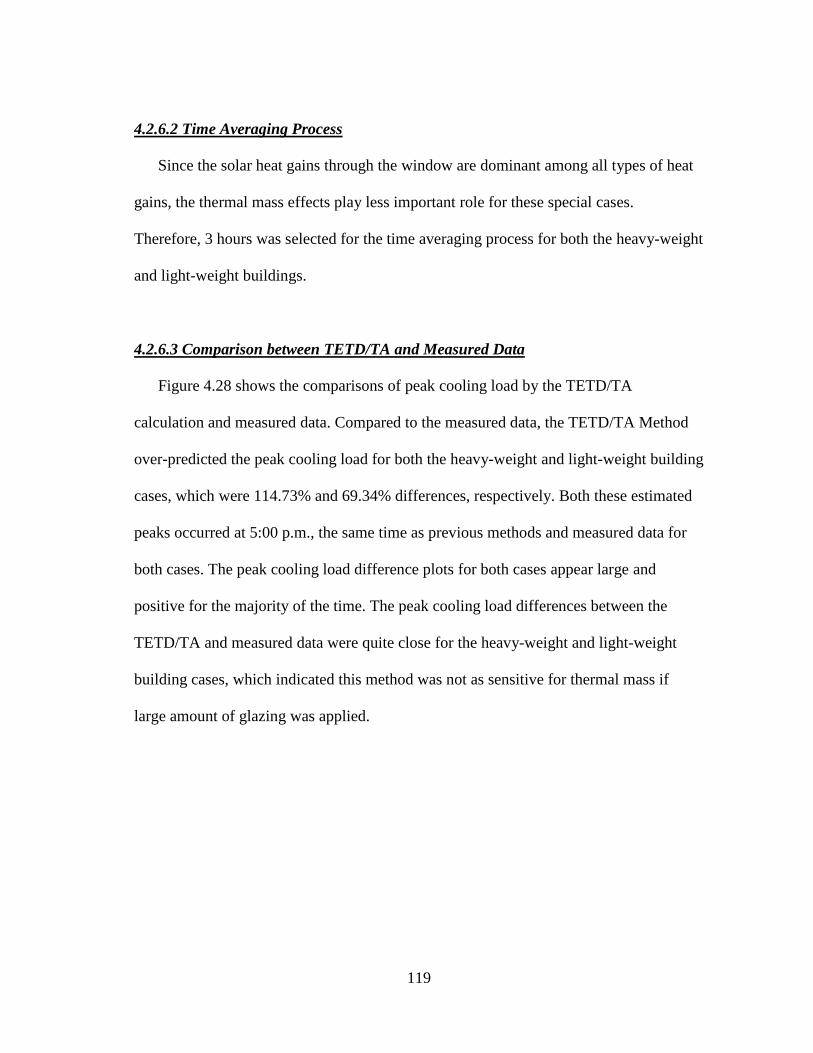
119
4.2.6.2 Time Averaging Process
Since the solar heat gains through the window are dominant among all types of heat
gains, the thermal mass effects play less important role for these special cases.
Therefore, 3 hours was selected for the time averaging process for both the heavy-weight
and light-weight buildings.
4.2.6.3 Comparison between TETD/TA and Measured Data
Figure 4.28 shows the comparisons of peak cooling load by the TETD/TA
calculation and measured data. Compared to the measured data, the TETD/TA Method
over-predicted the peak cooling load for both the heavy-weight and light-weight building
cases, which were 114.73% and 69.34% differences, respectively. Both these estimated
peaks occurred at 5:00 p.m., the same time as previous methods and measured data for
both cases. The peak cooling load difference plots for both cases appear large and
positive for the majority of the time. The peak cooling load differences between the
TETD/TA and measured data were quite close for the heavy-weight and light-weight
building cases, which indicated this method was not as sensitive for thermal mass if
large amount of glazing was applied.
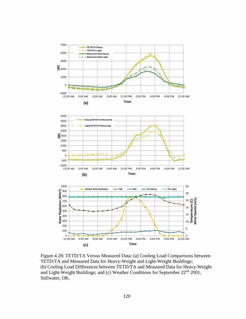
120
-1500
0
1500
3000
4500
6000
7500
12:00 AM 3:00 AM 6:00 AM 9:00 AM 12:00 PM 3:00 PM 6:00 PM 9:00 PM 12:00 AM
(W)
Time
TETD/TA-Heavy
TETD/TA-Light
Measured Data-Heavy
Measured Data-Light
(a)
-1000
-500
0
500
1000
1500
2000
2500
3000
3500
4000
12:00 AM 3:00 AM 6:00 AM 9:00 AM 12:00 PM 3:00 PM 6:00 PM 9:00 PM 12:00 AM
(W)
Time
Heavy(TETD/TA-Measured)
Light(TETD/TA-Measured)
(b)(b)
0
5
10
15
20
25
30
35
0
100
200
300
400
500
600
700
800
900
1000
12:00 AM 3:00 AM 6:00 AM 9:00 AM 12:00 PM 3:00 PM 6:00 PM 9:00 PM 12:00 AM
Te
mp
era
ture
(C
)W
ind
Sp
ee
d (
m/s
)
So
lar
Ra
dia
tio
n (
W/m
2)
Time
Global Solar Radiation Tdb WS Tin-Heavy Tin-Light
(c)
Figure 4.28: TETD/TA Versus Measured Data: (a) Cooling Load Comparisons between
TETD/TA and Measured Data for Heavy-Weight and Light-Weight Buildings;
(b) Cooling Load Differences between TETD/TA and Measured Data for Heavy-Weight
and Light-Weight Buildings; and (c) Weather Conditions for September 22nd 2001,
Stillwater, OK.
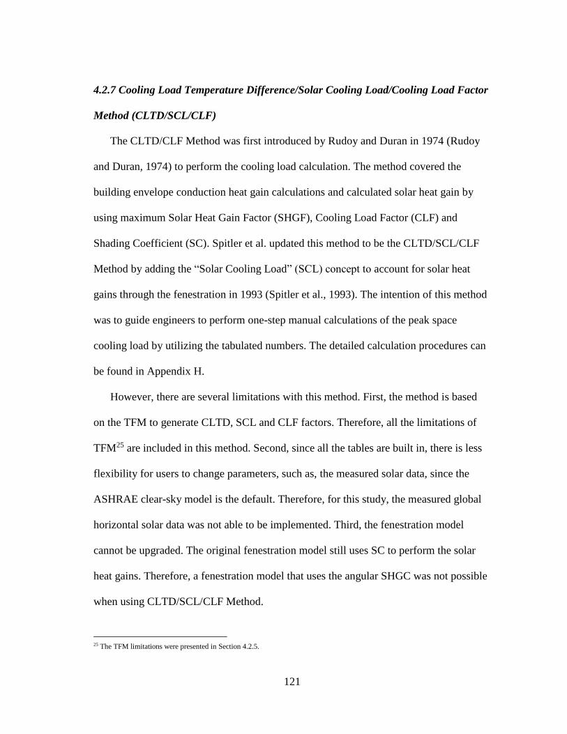
121
4.2.7 Cooling Load Temperature Difference/Solar Cooling Load/Cooling Load Factor
Method (CLTD/SCL/CLF)
The CLTD/CLF Method was first introduced by Rudoy and Duran in 1974 (Rudoy
and Duran, 1974) to perform the cooling load calculation. The method covered the
building envelope conduction heat gain calculations and calculated solar heat gain by
using maximum Solar Heat Gain Factor (SHGF), Cooling Load Factor (CLF) and
Shading Coefficient (SC). Spitler et al. updated this method to be the CLTD/SCL/CLF
Method by adding the “Solar Cooling Load” (SCL) concept to account for solar heat
gains through the fenestration in 1993 (Spitler et al., 1993). The intention of this method
was to guide engineers to perform one-step manual calculations of the peak space
cooling load by utilizing the tabulated numbers. The detailed calculation procedures can
be found in Appendix H.
However, there are several limitations with this method. First, the method is based
on the TFM to generate CLTD, SCL and CLF factors. Therefore, all the limitations of
TFM25 are included in this method. Second, since all the tables are built in, there is less
flexibility for users to change parameters, such as, the measured solar data, since the
ASHRAE clear-sky model is the default. Therefore, for this study, the measured global
horizontal solar data was not able to be implemented. Third, the fenestration model
cannot be upgraded. The original fenestration model still uses SC to perform the solar
heat gains. Therefore, a fenestration model that uses the angular SHGC was not possible
when using CLTD/SCL/CLF Method.
25 The TFM limitations were presented in Section 4.2.5.

122
4.2.7.1 Cooling Load from Conduction Heat Gains
Similar to the TFM, the proper determination of walls/roof group numbers is
required for all calculations. Different from the TFM, the tabulated walls/roofs are
further regrouped. In the method, a total of 16 wall and 10 roof numbers are available for
users to select. Table 4.13 shows the walls/roofs group number selections for heavy-
weight and light-weight buildings.
Table 4.13: Group Selections of Heavy-Weight and Light-Weight Buildings
Heavy-Weight Building Light-Weight Building
Wall Roof Wall Roof
Principal Material C18 C12 B7 B7
Secondary Material A2 - A1 -
Mass Location Mass in Mass in Mass integral Mass integral
R-Value 6.37 16.56 20.04 13.39
Group No. 16 4 4 2
The CLTD is used for calculating conduction heat gains and the tables need to be
updated for various design month and latitude. The case study site was located at 36.1
N latitude and the design day was September 22nd, 2001. Unfortunately, the tables were
not available from ASHRAE Handbook of Fundamentals (ASHRAE, 1997). Therefore,
the “CLTDTAB.EXE26” was used for generating the desired tables for September that
are shown in Figure 4.29 - Figure 4.31. In these tables, the top row represents the solar
time of the peak day. Note this was not local time and should be paid attention to during
the calculations. By selecting proper walls/roofs numbers and orientation for the walls,
the tabulated CLTD was obtained. However, an adjustment was needed to be made
26 The CLTDTAB.EXE only generates the tables in IP unit. The IP tables was converted to SI units and used in the calculations.
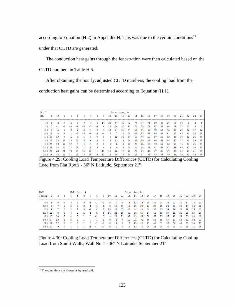
123
according to Equation (H.2) in Appendix H. This was due to the certain conditions27
under that CLTD are generated.
The conduction heat gains through the fenestration were then calculated based on the
CLTD numbers in Table H.5.
After obtaining the hourly, adjusted CLTD numbers, the cooling load from the
conduction heat gains can be determined according to Equation (H.1).
Figure 4.29: Cooling Load Temperature Differences (CLTD) for Calculating Cooling
Load from Flat Roofs - 36 N Latitude, September 21st.
Figure 4.30: Cooling Load Temperature Differences (CLTD) for Calculating Cooling
Load from Sunlit Walls, Wall No.4 - 36 N Latitude, September 21st.
27 The conditions are shown in Appendix H.

124
Figure 4.31: Cooling Load Temperature Differences (CLTD) for Calculating Cooling
Load from Sunlit Walls, Wall No.16 - 36 N Latitude, September 21st.
4.2.7.2 Cooling Load from Solar Heat Gains
The cooling load calculation from the solar heat gain through the window relies on
the Solar Cooling Load (SCL). The SCL also varies by the design month and latitude. To
choose the proper SCL tables, the zone type needed to first be determined. According to
Table H.6, Zone Type A was the closest selection for both the heavy-weight and light-
weight buildings. By running “CLTDTAB.EXE” program, the SCL tables for 36 N
latitude and September 21st were generated, shown in Figure 4.32. Using the proper
glass facing orientation (i.e., N represents North), the proper hourly SCL was obtained.
Next, using Equations (H.4) and (H.5), the cooling load from solar heat gains through
the fenestration was calculated.
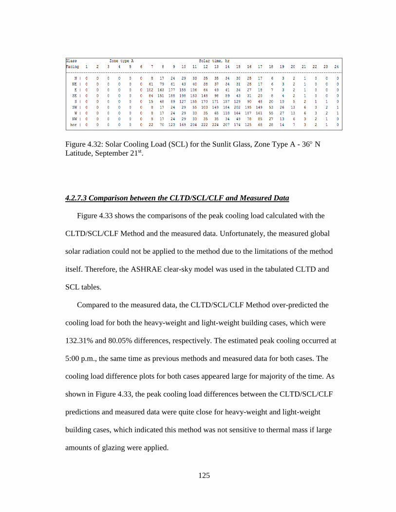
125
Figure 4.32: Solar Cooling Load (SCL) for the Sunlit Glass, Zone Type A - 36 N
Latitude, September 21st.
4.2.7.3 Comparison between the CLTD/SCL/CLF and Measured Data
Figure 4.33 shows the comparisons of the peak cooling load calculated with the
CLTD/SCL/CLF Method and the measured data. Unfortunately, the measured global
solar radiation could not be applied to the method due to the limitations of the method
itself. Therefore, the ASHRAE clear-sky model was used in the tabulated CLTD and
SCL tables.
Compared to the measured data, the CLTD/SCL/CLF Method over-predicted the
cooling load for both the heavy-weight and light-weight building cases, which were
132.31% and 80.05% differences, respectively. The estimated peak cooling occurred at
5:00 p.m., the same time as previous methods and measured data for both cases. The
cooling load difference plots for both cases appeared large for majority of the time. As
shown in Figure 4.33, the peak cooling load differences between the CLTD/SCL/CLF
predictions and measured data were quite close for heavy-weight and light-weight
building cases, which indicated this method was not sensitive to thermal mass if large
amounts of glazing were applied.
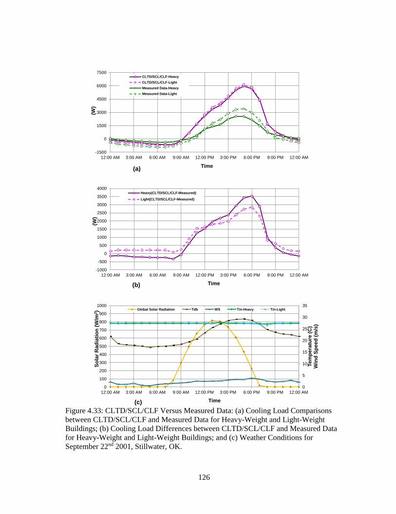
126
-1500
0
1500
3000
4500
6000
7500
12:00 AM 3:00 AM 6:00 AM 9:00 AM 12:00 PM 3:00 PM 6:00 PM 9:00 PM 12:00 AM
(W)
Time
CLTD/SCL/CLF-Heavy
CLTD/SCL/CLF-Light
Measured Data-Heavy
Measured Data-Light
(a)
-1000
-500
0
500
1000
1500
2000
2500
3000
3500
4000
12:00 AM 3:00 AM 6:00 AM 9:00 AM 12:00 PM 3:00 PM 6:00 PM 9:00 PM 12:00 AM
(W)
Time
Heavy(CLTD/SCL/CLF-Measured)
Light(CLTD/SCL/CLF-Measured)
(b)(b)
0
5
10
15
20
25
30
35
0
100
200
300
400
500
600
700
800
900
1000
12:00 AM 3:00 AM 6:00 AM 9:00 AM 12:00 PM 3:00 PM 6:00 PM 9:00 PM 12:00 AM
Tem
pera
ture
(C
)W
ind
Sp
ee
d (
m/s
)
So
lar
Rad
iati
on
(W
/m2)
Time
Global Solar Radiation Tdb WS Tin-Heavy Tin-Light
(c) Figure 4.33: CLTD/SCL/CLF Versus Measured Data: (a) Cooling Load Comparisons
between CLTD/SCL/CLF and Measured Data for Heavy-Weight and Light-Weight
Buildings; (b) Cooling Load Differences between CLTD/SCL/CLF and Measured Data
for Heavy-Weight and Light-Weight Buildings; and (c) Weather Conditions for
September 22nd 2001, Stillwater, OK.
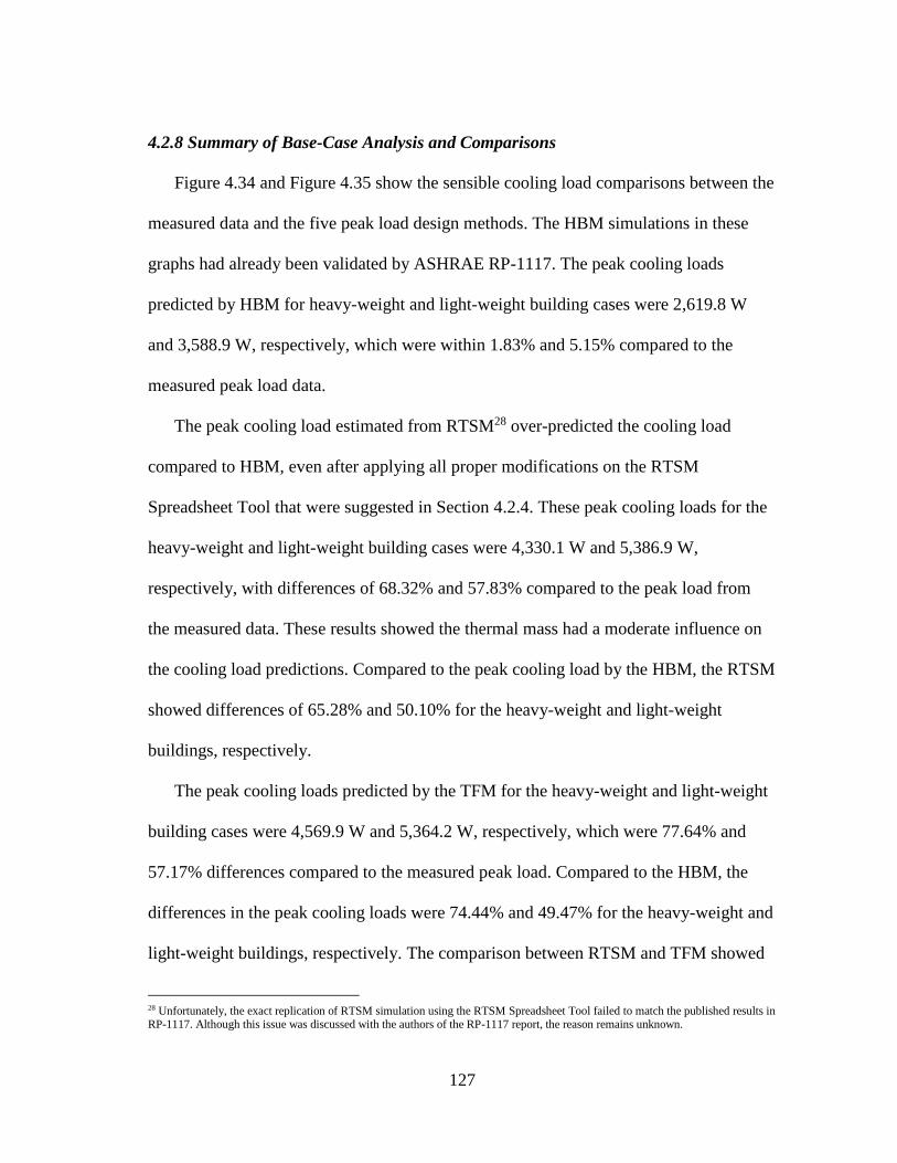
127
4.2.8 Summary of Base-Case Analysis and Comparisons
Figure 4.34 and Figure 4.35 show the sensible cooling load comparisons between the
measured data and the five peak load design methods. The HBM simulations in these
graphs had already been validated by ASHRAE RP-1117. The peak cooling loads
predicted by HBM for heavy-weight and light-weight building cases were 2,619.8 W
and 3,588.9 W, respectively, which were within 1.83% and 5.15% compared to the
measured peak load data.
The peak cooling load estimated from RTSM28 over-predicted the cooling load
compared to HBM, even after applying all proper modifications on the RTSM
Spreadsheet Tool that were suggested in Section 4.2.4. These peak cooling loads for the
heavy-weight and light-weight building cases were 4,330.1 W and 5,386.9 W,
respectively, with differences of 68.32% and 57.83% compared to the peak load from
the measured data. These results showed the thermal mass had a moderate influence on
the cooling load predictions. Compared to the peak cooling load by the HBM, the RTSM
showed differences of 65.28% and 50.10% for the heavy-weight and light-weight
buildings, respectively.
The peak cooling loads predicted by the TFM for the heavy-weight and light-weight
building cases were 4,569.9 W and 5,364.2 W, respectively, which were 77.64% and
57.17% differences compared to the measured peak load. Compared to the HBM, the
differences in the peak cooling loads were 74.44% and 49.47% for the heavy-weight and
light-weight buildings, respectively. The comparison between RTSM and TFM showed
28 Unfortunately, the exact replication of RTSM simulation using the RTSM Spreadsheet Tool failed to match the published results in RP-1117. Although this issue was discussed with the authors of the RP-1117 report, the reason remains unknown.

128
peak cooling load differences of 5.54% and -0.42% for the heavy-weight and light-
weight buildings, respectively. This indicated that the peak cooling load calculated by
the RTSM and the TFM give similar peak cooling load values. The large differences in
the sensible cooling loads occurred from 12:00 p.m. to 7:00 p.m. for both TFM and
HBM comparison. However, for the afternoon, the RTSM predicted a higher cooling
load than the cooling load predicted by the TFM. During the evening, the TFM tended to
predict a larger space cooling load.
The peak cooling loads calculated by the TETD/TA Method for the heavy-weight
and light-weight building cases were 5,524.1 W and 5,779.7 W, respectively, which
represented differences of 114.73% and 69.34% compared to the peak load from the
measured data. Compared to the HBM, the differences in the peak cooling load were
110.86% and 61.04% for the heavy-weight and light-weight buildings, respectively. The
comparison between the RTSM and the TETD/TA showed peak cooling load differences
of 27.57% and 7.29% for the heavy-weight and light-weight buildings, respectively.
Furthermore, compared with the TFM, the peak cooling load differences were 20.88%
and 7.75% for the heavy-weight and light-weight buildings, respectively.
The peak cooling loads calculated by the CLTD/SCL/CLF Method for the heavy-
weight and light-weight building cases were 5,976.3 W and 6,145.2 W, respectively,
which represented 132.31% and 80.5% differences compared to the measured peak
loads. Compared to the HBM, the differences in the peak cooling load were 128.12%
and 71.23% for the heavy-weight and light-weight buildings, respectively. The
comparison between the RTSM and the TETD/TA showed peak cooling load differences
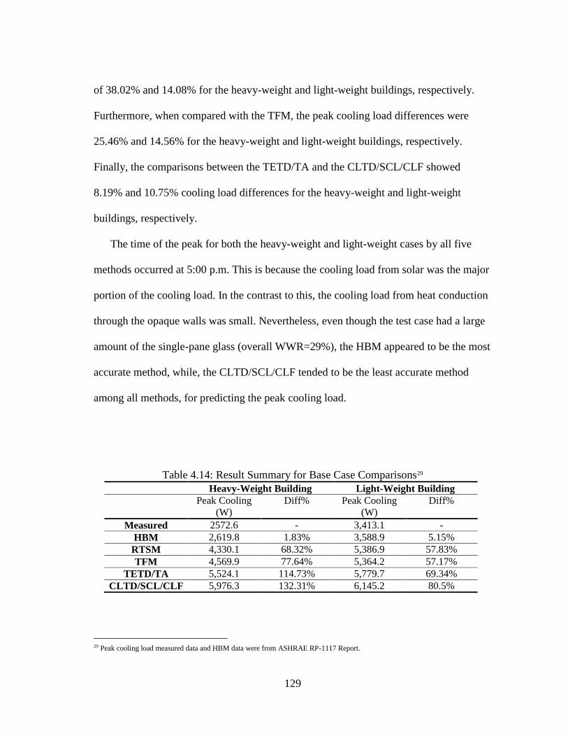
129
of 38.02% and 14.08% for the heavy-weight and light-weight buildings, respectively.
Furthermore, when compared with the TFM, the peak cooling load differences were
25.46% and 14.56% for the heavy-weight and light-weight buildings, respectively.
Finally, the comparisons between the TETD/TA and the CLTD/SCL/CLF showed
8.19% and 10.75% cooling load differences for the heavy-weight and light-weight
buildings, respectively.
The time of the peak for both the heavy-weight and light-weight cases by all five
methods occurred at 5:00 p.m. This is because the cooling load from solar was the major
portion of the cooling load. In the contrast to this, the cooling load from heat conduction
through the opaque walls was small. Nevertheless, even though the test case had a large
amount of the single-pane glass (overall WWR=29%), the HBM appeared to be the most
accurate method, while, the CLTD/SCL/CLF tended to be the least accurate method
among all methods, for predicting the peak cooling load.
Table 4.14: Result Summary for Base Case Comparisons29
Heavy-Weight Building Light-Weight Building
Peak Cooling
(W)
Diff% Peak Cooling
(W)
Diff%
Measured 2572.6 - 3,413.1 -
HBM 2,619.8 1.83% 3,588.9 5.15%
RTSM 4,330.1 68.32% 5,386.9 57.83%
TFM 4,569.9 77.64% 5,364.2 57.17%
TETD/TA 5,524.1 114.73% 5,779.7 69.34%
CLTD/SCL/CLF 5,976.3 132.31% 6,145.2 80.5%
29 Peak cooling load measured data and HBM data were from ASHRAE RP-1117 Report.
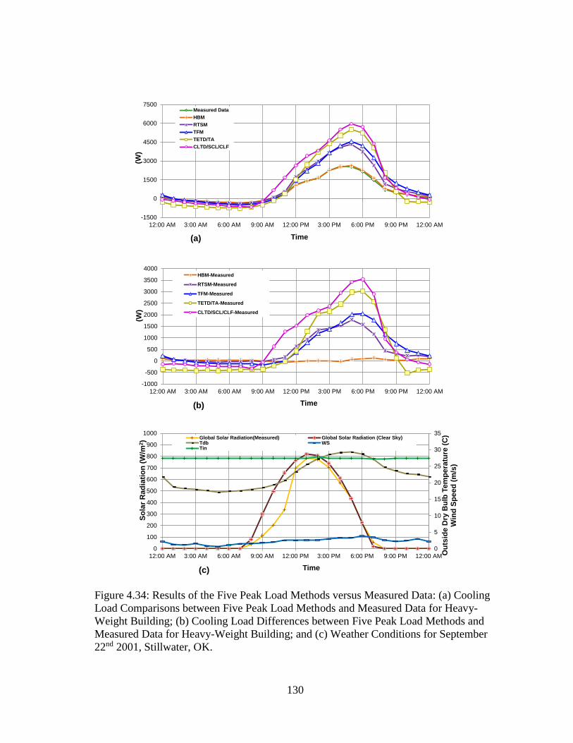
130
-1500
0
1500
3000
4500
6000
7500
12:00 AM 3:00 AM 6:00 AM 9:00 AM 12:00 PM 3:00 PM 6:00 PM 9:00 PM 12:00 AM
(W)
Time
Measured Data
HBM
RTSM
TFM
TETD/TA
CLTD/SCL/CLF
-1000
-500
0
500
1000
1500
2000
2500
3000
3500
4000
12:00 AM 3:00 AM 6:00 AM 9:00 AM 12:00 PM 3:00 PM 6:00 PM 9:00 PM 12:00 AM
(W)
Time
HBM-Measured
RTSM-Measured
TFM-Measured
TETD/TA-Measured
CLTD/SCL/CLF-Measured
(b)(b)(b)(b)(b)
(a)
0
5
10
15
20
25
30
35
0
100
200
300
400
500
600
700
800
900
1000
12:00 AM 3:00 AM 6:00 AM 9:00 AM 12:00 PM 3:00 PM 6:00 PM 9:00 PM 12:00 AM Ou
tsid
e D
ry B
ulb
Te
mp
era
ture
(C
)W
ind
Sp
ee
d (
m/s
)
So
lar
Ra
dia
tio
n (
W/m
2)
Time
Global Solar Radiation(Measured) Global Solar Radiation (Clear Sky)Tdb WSTin
(c)
Figure 4.34: Results of the Five Peak Load Methods versus Measured Data: (a) Cooling
Load Comparisons between Five Peak Load Methods and Measured Data for Heavy-
Weight Building; (b) Cooling Load Differences between Five Peak Load Methods and
Measured Data for Heavy-Weight Building; and (c) Weather Conditions for September
22nd 2001, Stillwater, OK.

131
-1500
0
1500
3000
4500
6000
7500
12:00 AM 3:00 AM 6:00 AM 9:00 AM 12:00 PM 3:00 PM 6:00 PM 9:00 PM 12:00 AM
(W)
Time
Measured Data
HBM
RTSM
TFM
TETD/TA
CLTD/SCL/CLF
(a)
-1000
-500
0
500
1000
1500
2000
2500
3000
3500
4000
12:00 AM 3:00 AM 6:00 AM 9:00 AM 12:00 PM 3:00 PM 6:00 PM 9:00 PM 12:00 AM
(W)
Time
HBM-Measured
RTSM-Measured
TFM-Measured
TETD/TA-Measured
CLTD/SCL/CLF-Measured
(b)(b)(b)(b)(b)
0
5
10
15
20
25
30
35
0
100
200
300
400
500
600
700
800
900
1000
12:00 AM 3:00 AM 6:00 AM 9:00 AM 12:00 PM 3:00 PM 6:00 PM 9:00 PM 12:00 AM Ou
tsid
e D
ry B
ulb
Te
mp
era
ture
(C
)W
ind
Sp
ee
d (
m/s
)
So
lar
Ra
dia
tio
n (
W/m
2)
Time
Global Solar Radiation(Measured) Global Solar Radiation (Clear Sky)Tdb WSTin
(c)
Figure 4.35: Results of the Five Peak Load Methods versus Measured Data: (a) Cooling
Load Comparisons between Five Peak Load Methods and Measured Data for Light-
Weight Building; (b) Cooling Load Differences between Five Peak Load Methods and
Measured Data for Light-Weight Building; and (c) Weather Conditions for September
22nd 2001, Stillwater, OK.
132
4.3 Part III: Additional Case-Study Comparison of the Peak Cooling Load Design
Methods
This section aims to provide additional case-study analysis to further compare the
five methods used to predict the peak sensible cooling load. To accomplish this, the two
parameters were varied, including the window area and glazing types. The south and
west window areas were always kept the same whenever the window area increased or
decreased, according to the percentage of respective wall 11.15 m2. Fifteen cases were
analyzed, as shown in Table 4.15, which included different types and areas of glazing.
All parameters were applied to both the heavy-weight and light-weight building cases.
Since measured data for all the variations were not available, the simulation results
by the HBM were regarded as the baseline to be compared with the peak cooling load
calculations from the RTSM, the TFM, the TETD/TA Method, and the CLTD/SCL/CLF
Method.
4.3.1 Observations for Peak Cooling Load Comparisons by All Methods
Figure 4.36 and Figure 4.37 show the comparisons of the RTSM, the TFM, the
TETD/TA Method, and the CLTD/SCL/CLF Method for both heavy-weight and light-
weight building cases, respectively. The X-axis shows the test case numbers and Y-axis
shows the differences with respect to the HBM.

133
Table 4.15: Test Case Descriptions
Test
Case
No.
Glazing
Type
U-Value
(W/m2-
K)
Normal
SHGC
Each
Window %
to
Respective
Wall
Overall
WWR
Overall
WFR
South
Window
Area (m2)
West
Window
Area (m2)
Base
Case
Single
Pane
Clear
4.65 0.86 58% 29% 96% 6.45 6.45
TC1 Single
Pane
Clear
4.65 0.86
10% 5% 17% 1.12 1.12
TC2 30% 15% 50% 3.35 3.35
TC3 50% 25% 83% 5.58 5.58
TC4 Double
Pane
Clear
2.73 0.76
10% 5% 17% 1.12 1.12
TC5 30% 15% 50% 3.35 3.35
TC6 50% 25% 83% 5.58 5.58
TC7 Double
Pane
Low-e
1.99 0.70
10% 5% 17% 1.12 1.12
TC8 30% 15% 50% 3.35 3.35
TC9 50% 25% 83% 5.58 5.58
TC10 Triple
Pane
Clear
1.76 0.68
10% 5% 17% 1.12 1.12
TC11 30% 15% 50% 3.35 3.35
TC12 50% 25% 83% 5.58 5.58
TC13 Triple
Pane
Low-e
1.87 0.62
10% 5% 17% 1.12 1.12
TC14 30% 15% 50% 3.35 3.35
TC15 50% 25% 83% 5.58 5.58
The following were observed for the heavy-weight building test cases:
For all the heavy-weight building test cases, it appeared that the predicted peak
cooling loads from the four simplified methods for the 15% WWR were the closest to
the results from the cooling load calculated by the HBM;
For heavy-weight building, the test cases with a 5% WWR underestimated the
peak cooling loads by all four methods compared to the HBM, while the test cases with a
25% WWR over-predicted the cooling loads;
Across all types of window glazing, the peak cooling load of the test case 12,
with a 25% WWR and triple pane clear windows, by the RTSM was 0.83% different
compared to the HBM, which was considered the best match between the RTSM and
HBM for all heavy-weight building case simulation;
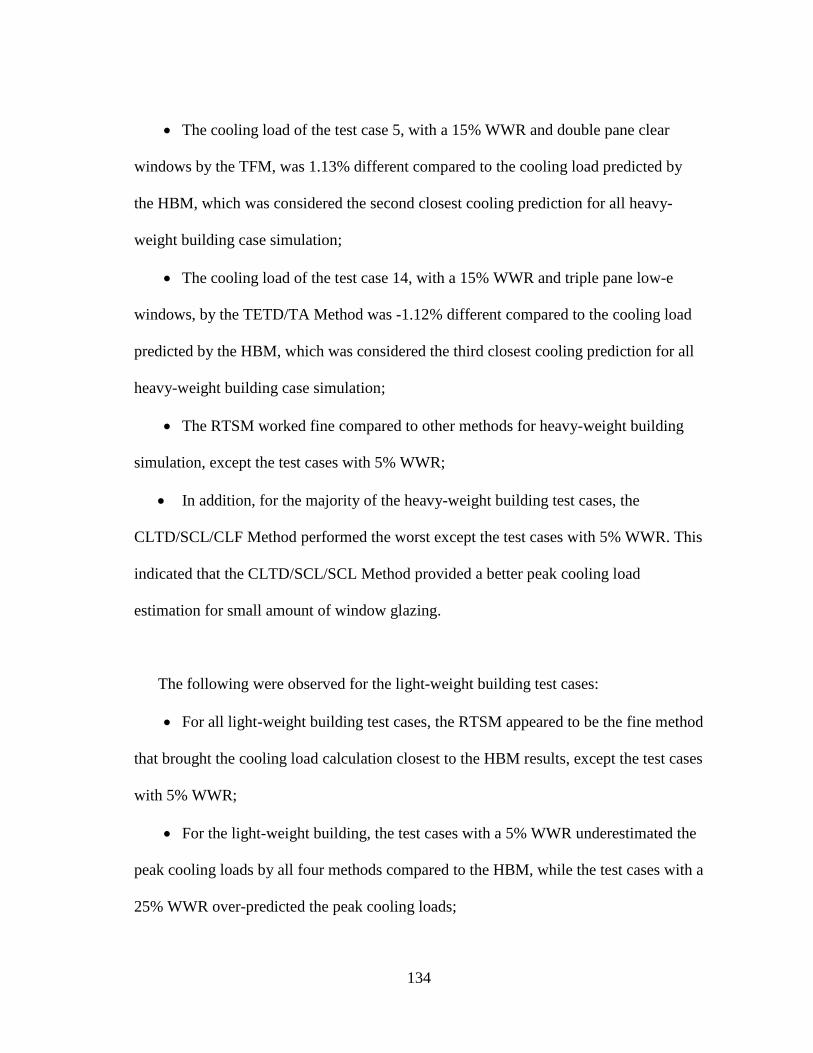
134
The cooling load of the test case 5, with a 15% WWR and double pane clear
windows by the TFM, was 1.13% different compared to the cooling load predicted by
the HBM, which was considered the second closest cooling prediction for all heavy-
weight building case simulation;
The cooling load of the test case 14, with a 15% WWR and triple pane low-e
windows, by the TETD/TA Method was -1.12% different compared to the cooling load
predicted by the HBM, which was considered the third closest cooling prediction for all
heavy-weight building case simulation;
The RTSM worked fine compared to other methods for heavy-weight building
simulation, except the test cases with 5% WWR;
In addition, for the majority of the heavy-weight building test cases, the
CLTD/SCL/CLF Method performed the worst except the test cases with 5% WWR. This
indicated that the CLTD/SCL/SCL Method provided a better peak cooling load
estimation for small amount of window glazing.
The following were observed for the light-weight building test cases:
For all light-weight building test cases, the RTSM appeared to be the fine method
that brought the cooling load calculation closest to the HBM results, except the test cases
with 5% WWR;
For the light-weight building, the test cases with a 5% WWR underestimated the
peak cooling loads by all four methods compared to the HBM, while the test cases with a
25% WWR over-predicted the peak cooling loads;
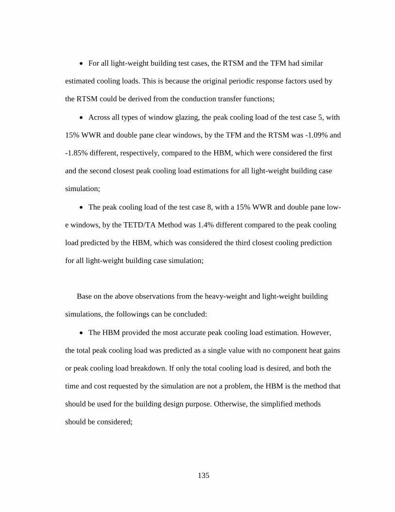
135
For all light-weight building test cases, the RTSM and the TFM had similar
estimated cooling loads. This is because the original periodic response factors used by
the RTSM could be derived from the conduction transfer functions;
Across all types of window glazing, the peak cooling load of the test case 5, with
15% WWR and double pane clear windows, by the TFM and the RTSM was -1.09% and
-1.85% different, respectively, compared to the HBM, which were considered the first
and the second closest peak cooling load estimations for all light-weight building case
simulation;
The peak cooling load of the test case 8, with a 15% WWR and double pane low-
e windows, by the TETD/TA Method was 1.4% different compared to the peak cooling
load predicted by the HBM, which was considered the third closest cooling prediction
for all light-weight building case simulation;
Base on the above observations from the heavy-weight and light-weight building
simulations, the followings can be concluded:
The HBM provided the most accurate peak cooling load estimation. However,
the total peak cooling load was predicted as a single value with no component heat gains
or peak cooling load breakdown. If only the total cooling load is desired, and both the
time and cost requested by the simulation are not a problem, the HBM is the method that
should be used for the building design purpose. Otherwise, the simplified methods
should be considered;

136
For the majority of test cases, the RTSM worked fairly well, which allows its
recommendation for use if the HBM cannot be performed;
The second recommended simplified method is the TFM, since it can provide
similar results to the RTSM simulation;
The TETD/TA Method provides the next best results;
The least accurate method is the CLTD/SCL/CLF Method.
Details regarding the sensible cooling load comparisons are presented in Appendix I.
4.3.2 Observations about the Test Case Comparisons for Each Method
Figure 4.38 - Figure 4.42 show the case study analysis comparisons by the HBM, the
RTSM, the TFM, the TETD/TA Method and the CLTD/SCL/CLF Method for both
heavy-weight and light-weight building cases. Due to the thermal mass effects, the peak
cooling load for the light-weight building for all test cases tended to produce higher peak
cooling load than the heavy-weight building cases.
The RTSM, the TFM, the TETD/TA Method and the CLTD/SCL/CLF Method all
are quite sensitive to the glazing areas and glazing types. In contrast, the HBM is quite
steady and predicts the peak cooling load well within a certain range. For all methods,
either the more efficient window glazing or the smaller window areas the lower peak
cooling load are demonstrated.

137
-100%
-50%
0%
50%
100%
150%
TC1 TC2 TC3 TC4 TC5 TC6 TC7 TC8 TC9 TC10 TC11 TC12 TC13 TC14 TC15
(%)
Test CaseRTSM TFM TETD/TA CLTD/SCL/CLF
Double Pane Double Pane Low-e Triple Pane TriplePane Low-eDouble Pane Double Pane Low-e Triple Pane TriplePane Low-eSingle Pane
Figure 4.36: Comparison of the Heavy-Weight Building Test Cases
-100%
-50%
0%
50%
100%
150%
TC1 TC2 TC3 TC4 TC5 TC6 TC7 TC8 TC9 TC10 TC11 TC12 TC13 TC14 TC15
(%)
Test CaseRTSM TFM TETD/TA CLTD/SCL/CLF
Double Pane Double Pane Low-e Triple Pane TriplePane Low-eSingle Pane
Figure 4.37: Comparison of the Light-Weight Building Test Cases
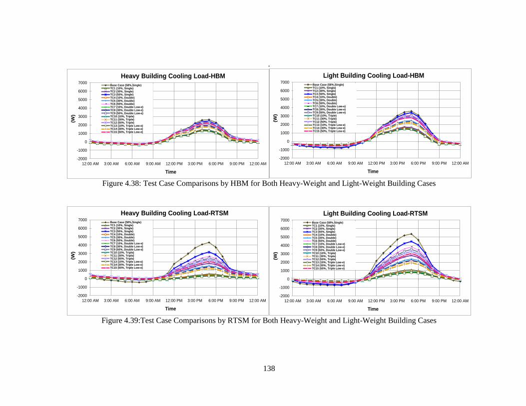
138
.
-2000
-1000
0
1000
2000
3000
4000
5000
6000
7000
12:00 AM 3:00 AM 6:00 AM 9:00 AM 12:00 PM 3:00 PM 6:00 PM 9:00 PM 12:00 AM
(W)
Time
Heavy Building Cooling Load-HBM
Base Case (58%,Single)TC1 (10%, Single)TC2 (30%, Single)TC3 (50%, Single)TC4 (10%, Double)TC5 (30%, Double)TC6 (50%, Double)TC7 (10%, Double Low-e)TC8 (30%, Double Low-e)TC9 (50%, Double Low-e)TC10 (10%, Triple)TC11 (30%, Triple)TC12 (50%, Triple)TC13 (10%, Triple Low-e)TC14 (30%, Triple Low-e)TC15 (50%, Triple Low-e)
-2000
-1000
0
1000
2000
3000
4000
5000
6000
7000
12:00 AM 3:00 AM 6:00 AM 9:00 AM 12:00 PM 3:00 PM 6:00 PM 9:00 PM 12:00 AM
(W)
Time
Light Building Cooling Load-HBM
Base Case (58%,Single)TC1 (10%, Single)TC2 (30%, Single)TC3 (50%, Single)TC4 (10%, Double)TC5 (30%, Double)TC6 (50%, Double)TC7 (10%, Double Low-e)TC8 (30%, Double Low-e)TC9 (50%, Double Low-e)TC10 (10%, Triple)TC11 (30%, Triple)TC12 (50%, Triple)TC13 (10%, Triple Low-e)TC14 (30%, Triple Low-e)TC15 (50%, Triple Low-e)
Figure 4.38: Test Case Comparisons by HBM for Both Heavy-Weight and Light-Weight Building Cases
-2000
-1000
0
1000
2000
3000
4000
5000
6000
7000
12:00 AM 3:00 AM 6:00 AM 9:00 AM 12:00 PM 3:00 PM 6:00 PM 9:00 PM 12:00 AM
(W)
Time
Heavy Building Cooling Load-RTSM
Base Case (58%,Single)TC1 (10%, Single)TC2 (30%, Single)TC3 (50%, Single)TC4 (10%, Double)TC5 (30%, Double)TC6 (50%, Double)TC7 (10%, Double Low-e)TC8 (30%, Double Low-e)TC9 (50%, Double Low-e)TC10 (10%, Triple)TC11 (30%, Triple)TC12 (50%, Triple)TC13 (10%, Triple Low-e)TC14 (30%, Triple Low-e)TC15 (50%, Triple Low-e)
-2000
-1000
0
1000
2000
3000
4000
5000
6000
7000
12:00 AM 3:00 AM 6:00 AM 9:00 AM 12:00 PM 3:00 PM 6:00 PM 9:00 PM 12:00 AM
(W)
Time
Light Building Cooling Load-RTSM
Base Case (58%,Single)TC1 (10%, Single)TC2 (30%, Single)TC3 (50%, Single)TC4 (10%, Double)TC5 (30%, Double)TC6 (50%, Double)TC7 (10%, Double Low-e)TC8 (30%, Double Low-e)TC9 (50%, Double Low-e)TC10 (10%, Triple)TC11 (30%, Triple)TC12 (50%, Triple)TC13 (10%, Triple Low-e)TC14 (30%, Triple Low-e)TC15 (50%, Triple Low-e)
Figure 4.39:Test Case Comparisons by RTSM for Both Heavy-Weight and Light-Weight Building Cases

139
-2000
-1000
0
1000
2000
3000
4000
5000
6000
7000
12:00 AM 3:00 AM 6:00 AM 9:00 AM 12:00 PM 3:00 PM 6:00 PM 9:00 PM 12:00 AM
(W)
Time
Heavy Building Cooling Load-TFM
Base Case (58%,Single)TC1 (10%, Single)TC2 (30%, Single)TC3 (50%, Single)TC4 (10%, Double)TC5 (30%, Double)TC6 (50%, Double)TC7 (10%, Double Low-e)TC8 (30%, Double Low-e)TC9 (50%, Double Low-e)TC10 (10%, Triple)TC11(30%, Triple)TC12 (50%, Triple)TC13 (10%, Triple Low-e)TC14 (30%, Triple Low-e)TC15 (50%, Triple Low-e)
-2000
-1000
0
1000
2000
3000
4000
5000
6000
7000
12:00 AM 3:00 AM 6:00 AM 9:00 AM 12:00 PM 3:00 PM 6:00 PM 9:00 PM 12:00 AM
(W)
Time
Light Building Cooling Load-TFM
Base Case (58%,Single)TC1 (10%, Single)TC2 (30%, Single)TC3 (50%, Single)TC4 (10%, Double)TC5 (30%, Double)TC6 (50%, Double)TC7 (10%, Double Low-e)TC8 (30%, Double Low-e)TC9 (50%, Double Low-e)TC10 (10%, Triple)TC11(30%, Triple)TC12 (50%, Triple)TC13 (10%, Triple Low-e)TC14 (30%, Triple Low-e)TC15 (50%, Triple Low-e)
Figure 4.40: Test Case Comparisons by TFM for Both Heavy-Weight and Light-Weight Building Cases
-2000
-1000
0
1000
2000
3000
4000
5000
6000
7000
12:00 AM 3:00 AM 6:00 AM 9:00 AM 12:00 PM 3:00 PM 6:00 PM 9:00 PM 12:00 AM
(W)
Time
Heavy Building Cooling Load-TETD/TA
Base Case (58%,Single)TC1 (10%, Single)TC2 (30%, Single)TC3 (50%, Single)TC4 (10%, Double)TC5 (30%, Double)TC6 (50%, Double)TC7 (10%, Double Low-e)TC8 (30%, Double Low-e)TC9 (50%, Double Low-e)TC10 (10%, Triple)TC11 (30%, Triple)TC12 (50%, Triple)TC13 (10%, Triple Low-e)TC14 (30%, Triple Low-e)TC15 (50%, Triple Low-e)
-2000
-1000
0
1000
2000
3000
4000
5000
6000
7000
12:00 AM 3:00 AM 6:00 AM 9:00 AM 12:00 PM 3:00 PM 6:00 PM 9:00 PM 12:00 AM
(W)
Time
Light Building Cooling Load-TETD/TA
Base Case (58%,Single)TC1 (10%, Single)TC2 (30%, Single)TC3 (50%, Single)TC4 (10%, Double)TC5 (30%, Double)TC6 (50%, Double)TC7 (10%, Double Low-e)TC8 (30%, Double Low-e)TC9 (50%, Double Low-e)TC10 (10%, Triple)TC11 (30%, Triple)TC12 (50%, Triple)TC13 (10%, Triple Low-e)TC14 (30%, Triple Low-e)TC15 (50%, Triple Low-e)
Figure 4.41: Test Case Comparisons by TETD/TA Method for Both Heavy-Weight and Light-Weight Building Cases
140
-2000
-1000
0
1000
2000
3000
4000
5000
6000
7000
12:00 AM 3:00 AM 6:00 AM 9:00 AM 12:00 PM 3:00 PM 6:00 PM 9:00 PM 12:00 AM
(W)
Time
Heavy Building Cooling Load-CLTD/SCL/CLF
Base Case (58%,Single)TC1 (10%, Single)TC2 (30%, Single)TC3 (50%, Single)TC4 (10%, Double)TC5 (30%, Double)TC6 (50%, Double)TC7 (10%, Double Low-e)TC8 (30%, Double Low-e)TC9 (50%, Double Low-e)TC10 (10%, Triple)TC11 (30%, Triple)TC12 (50%, Triple)TC13 (10%, Triple Low-e)TC14 (30%, Triple Low-e)TC15 (50%, Triple Low-e)
-2000
-1000
0
1000
2000
3000
4000
5000
6000
7000
12:00 AM 3:00 AM 6:00 AM 9:00 AM 12:00 PM 3:00 PM 6:00 PM 9:00 PM 12:00 AM
(W)
Time
Light Building Cooling Load-CLTD/SCL/CLF
Base Case (58%,Single)TC1 (10%, Single)TC2 (30%, Single)TC3 (50%, Single)TC4 (10%, Double)TC5 (30%, Double)TC6 (50%, Double)TC7 (10%, Double Low-e)TC8 (30%, Double Low-e)TC9 (50%, Double Low-e)TC10 (10%, Triple)TC11 (30%, Triple)TC12 (50%, Triple)TC13 (10%, Triple Low-e)TC14 (30%, Triple Low-e)TC15 (50%, Triple Low-e)
Figure 4.42: Test Case Comparisons by CLTD/SCL/CLF Method for Both Heavy-Weight and Light-Weight Building Cases
141
4.4 Summary
Chapter IV contained three sections of results of the study, including: survey and
interview; base case and additional test case analysis; and comparisons of the peak load
design methods. Five of the existing methods that are recognized by the engineers who
perform the load calculations including the HBM, the RTSM, the TFM, the TETD/TA
Method, and the CLTD/SCL/CLF Method were reviewed.
The analysis of the survey and interview provided a great insight into the general
building design process in the industry and the methods that are being used by the field
engineers to perform the peak cooling load calculations. There were eleven participants
in the survey. Nine of them continued with the interview process. The survey showed
that most of the participants used the CLTD/SCL/CLF Method since it is easy to use and
the accuracy is sufficient for their purpose. The RTSM, which is the only simplified
method existing in the 2013 ASHRAE Handbook of Fundamentals, was known by only
three of the participants. One of three said the RTSM could be used when it comes to
design LEED buildings. One said the RTSM was rarely used, and the last participant
was highly interested in using the RTSM. The TETD/TA Method was used by three of
the participants and the HBM was mentioned by two participants but not used. However,
only one participant knew about TFM, but is not currently using it. Since the number of
participants was small, the conclusions drawn from this study may have a bias, but, to
some extent, should reflect the industry uses peak cooling load methods in the peak
cooling load design.

142
A comparative analysis was performed based on the published data in the ASHRAE
RP-1117 report. In order to perform the study, the FORTRAN source codes for the
HBM was obtained from contacting authors of RP-1117 report (Fisher, 2015) and
recompiled by using the Elipse FORTRAN compiler. The HBM analysis was rerun and
compared to the published results in the RP-1117 report. The same sensible cooling load
output was obtained through this analysis. The efforts of duplicating the RTSM
simulations were performed using the 2009 ASHRAE RTSM Spreadsheet tool rather
than the LOADS Toolkit that was used in the RP-1117. Unfortunately, the sensible
cooling load estimated by the ASHRAE RTSM Spreadsheet tool showed a higher value
than the values that were published in RP-1117. Since no additional files were provided,
the reason for the differences remains unknown, despite the similar profiles. Compared
to the RP-1117 report that only covered the analysis of the HBM and the RTSM, the
current study performed additional analysis of the sensible cooling load of the heavy-
weight and light-weight building cases using the TFM, the TETD/TA Method, and the
CLTD/SCL/CLF Method to complete the comparisons. For both the heavy-weight and
light-weight building cases, the HBM was proved to be the most accurate method that
provided the closest peak cooling load estimation to the measured data. Although the
RTSM showed an over-prediction, it is still the best simplified method when compared
to the TFM, the TETD/TA Method, and the CLTD/SCL/CLF Method.
The TFM behaved similar to the RTSM and provided a slightly higher cooling load
peak, compared to the RTSM. The TETD/TA Method was the next most accurate.
However, this method included subjective information to perform the time averaging

143
process. Therefore, the results depend on the knowledge and background of the users of
this method.
Last but not least, the CLTD/SCL/CLF Method, not surprisingly, performed the
worst among all the methods. This is because a lot of assumptions were incorporated
when generating the CLTD, the SCL, and the CLF tables. Also, for the other four
methods, the measured solar data was used, which could not be performed for the
CLTD/SCL/CLF Method since it relied only on the published tables and no procedure
was provided to make the modifications to the published tables. In addition, the SC was
still used in fenestration model calculation of the CLTD/SCL/CLF Method for solar heat
gain calculations and was not upgraded to the fenestration model that uses SHGC.
In the current analysis, additional test cases that varied the window area and glazing
types were analyzed to further understand the differences between the five methods. In
this analysis, the HBM was used as a baseline due to the lack of measured data. For
windows with a small amount of glazing area, all simplified methods tended to
underestimate the sensible cooling load compared to the HBM. As more glazing was
added, a larger solar heat gain came into the space, which made all calculations over-
predict the sensible cooling load. Compared to the HBM, all the simplified methods
were sensitive to the parameters that could influence the solar heat gains. Their profile
seemed more spread out across all the test cases. This new set of analysis showed similar
conclusions as the base-case analysis, namely, the RTSM behaved the best. The TFM
was the next most accurate and showed close agreement with the RTSM. The TETD/TA

144
Method was the next in accuracy and the CLTD/SCL/CLF Method was the least
accurate.
When one combines the survey and interview results and all the comparison analysis,
the CLTD/SCL/CLF Method was most popular but gave the worst accuracy either
compared to the measured data or the HBM.
The survey and interview showed that the majority of the participants chose the easy-
to-use method rather than the more complicated methods even though the more complex
methods were more accurate. Based on this response, it was concluded that if greater
accuracy could be developed and demonstrated for the CLTD/SCL/CLF Method then
both the requirements of accuracy and simplicity could be achieved. The results of the
survey and interview conducted by this study agree with the seminar presentation by
Professor Walter Grondzik at the 2016 ASHRAE winter conference. In this presentation,
Professor Grondzik also recommended that ASHRAE provide a simple method like the
CLTD/SCL/CLF Method for architects to use (Grondzik, 2016).

145
CHAPTER V
PROPOSED ANALYSIS TO UPDATE THE SCL TABLES FOR THE
CLTD/SCL/CLF METHOD USING THE ASHRAE RTSM
SPREADSHEET TOOL
5.1 Overview
This Chapter provides a proposed analysis of updating the SCL tables for the
CLTD/SCL/CLF Method from the ASHRAE RTSM Spreadsheet Tool. This analysis
was motivated by both survey and interview and a detailed comparison of results against
the published RP-1117 data. The survey and interview revealed that the
CLTD/SCL/CLF Method was still being used by a majority of the participants during the
building peak cooling load design process due to the simplicity of its application and
acceptable accuracy of the method compared to other methods. The CLTD/SCL/CLF
Method most widely is used in the TRACE 700 software. Unfortunately, the comparison
of all the current methods against measured data showed the CLTD/SCL/CLF Method
performed the worst among all the methods. This is because the CLTD/SCL/CLF
Method relies on the published tables that include many assumptions from when they
were generated. As mentioned before, there is always a trade-off between the
convenience of the easy-to-use and the calculation accuracy. The CLTD/SCL/CLF
Method was originally designed as a manual method that intended to provide a simpler
procedure than the TFM. In the CLTD/SCL/CLF Method, the tables were calculated on
the basis of TFM calculation results. As previously discussed, the results of the

146
comparison process showed the RTSM was found to be the most accurate method
among all the simplified methods that provided results closet to the HBM and measured
data. Therefore, there is a need to upgrade the CLTD/SCL/CLF tables according to the
RTSM calculations to make it more accurate.
In the current study, the proposed analysis procedure to update the SCL tables is
demonstrated to show how the potential modifications of the CLTD/SCL/CLF Method
can be improved. The original SCL table used in the analysis was shown in Figure 4.32
in Chapter IV.
5.2 Analysis Procedure
As previously noted, the fenestration heat gain model in the CLTD/SCL/CLF
Method uses Shading Coefficient (SC) and Double Strength Glass (DSA) coefficients to
estimate the solar heat gains through the window (shown in Appendix C, Equations
(C.1)-(C.9)). After obtaining the new SCL numbers from the table, Equation (H.4) in the
Appendix H was used for solar cooling load calculations. In the 2013 ASHRAE
Handbook of Fundamentals, the fenestration heat gains are calculated using the SHGC
(shown in Equations (C.10) and (C.11)). Figure 5.1 shows the relationship and
connections between the two models.
For each glazing type, the angular-dependent SHGC can be obtained by multiplying
the SHGC at a normal incident angle by the published beam and diffuse SHGC angle
correction factors. The example of the correction factors are shown in Table 5.1. There

147
are total of 73 types of glazing with the associated SHGC correction factors in the
ASHRAE RTSM Spreadsheet Tool.
Table 5.1: SHGC Correction Factors (Adapted from Spitler, 2009)
ID Layer Normal
SHGC
SHGC Angle Correction Factors and Diffuse Correction
Factors
0 40 50 60 70 80 Diffuse
1A Clear 0.86 1 0.977 0.953 0.907 0.779 0.488 0.907
5A Clear/Clear 0.76 1 0.974 0.934 0.842 0.658 0.342 0.868
29A Clear/Clear/Clear 0.68 1 0.956 0.912 0.794 0.574 0.265 0.838
To begin with, according to the 2013 ASHRAE Handbook of Fundamentals, the
fenestration solar heat gains can be determined by using the following,
, ( ) ( , )b t bq AE SHGC IAC (5.1)
, ,( )d t d t r DDq A E E SHGC IAC (5.2)
where,
A : window surface area, m2;
,r bE : beam solar radiation falling on the fenestration, W/m2;
,t dE : diffuse solar radiation from the sky falling on the fenestration, W/m2;
,t rE : diffuse solar radiation from the ground reflection falling on the fenestration,
W/m2;
( )SHGC : incidence angle based beam solar heat gain coefficient;
DSHGC : diffuse solar heat gain coefficient;
( , )IAC : indoor solar attenuation coefficient for beam solar heat gain coefficient;
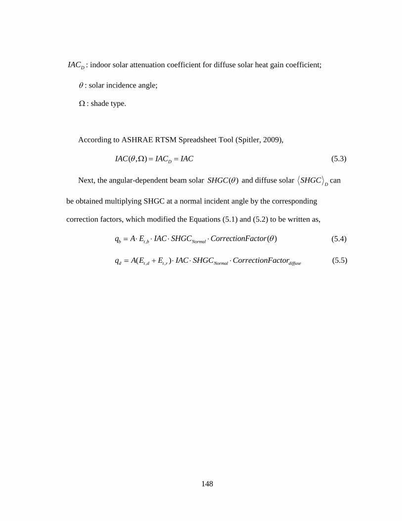
148
DIAC : indoor solar attenuation coefficient for diffuse solar heat gain coefficient;
: solar incidence angle;
: shade type.
According to ASHRAE RTSM Spreadsheet Tool (Spitler, 2009),
( , ) DIAC IAC IAC (5.3)
Next, the angular-dependent beam solar ( )SHGC and diffuse solar D
SHGC can
be obtained multiplying SHGC at a normal incident angle by the corresponding
correction factors, which modified the Equations (5.1) and (5.2) to be written as,
, ( )b t b Normalq A E IAC SHGC CorrectionFactor (5.4)
, ,( )d t d t r Normal diffuseq A E E IAC SHGC CorrectionFactor (5.5)

149
Transmitted Solar Heat Gains
Transmitted Beam Solar Heat Gains
Transmitted Diffuse Solar Heat Gains
Inwarding Absorbed Solar Heat Gains
Inwarding Absorbed Beam Solar Heat Gains
Inwarding Absorbed Diffuse Solar Heat Gains
Fenestration Solar Heat Gain Model 1
DS
A G
lass C
oefficien
ts for C
alcu
latin
g T
ran
smitta
nce a
nd
Ab
sorp
tan
ce
To
tal F
en
estratio
n S
ola
r Hea
t Ga
ins
∑ S
ola
r Hea
t ga
ins ∙S
C∙A
Beam Solar Heat Gains
Beam Transmitted Solar Heat Gains
Beam Inwarding Absorbed Solar Heat
Gains
Diffuse Solar Heat Gains
Diffuse Transmitted Solar Heat Gains
Diffuse Inwarding Absorbed Solar Heat Gains
Fenestration Solar Heat Gain Model 2
Incid
ence A
ng
le Ba
sed S
HG
C fo
r Gla
zing
Ty
pes
To
tal F
en
estratio
n S
ola
r Hea
t Ga
ins
∑ S
ola
r Hea
t ga
ins ∙IA
C∙A
Figure 5.1: Relationship and Connections between Two Fenestration Heat Gain Calculation Models

150
By applying RTSM principles shown in Appendix E, the sensible cooling load from
fenestration solar heat gains can be given as,
23 23
, , , ,
0 0
23
, ,
0
, , ,
( ) ( )
{ [ ( )] }
{ [ ( ) ] }
Solar solar i b i non solar j d j
i j
solar i t b Normal i
i
non solar j t d t r Normal diffuse j
j
Q r q r q
r A E IAC SHGC CorrectionFactor
r A E E IAC SHGC CorrectionFactor
23
0
23
, ,
0
23
, , ,
0
{ [ ( )] }
{ [( ) ] }
isolar i t b
i
Normal
non solar j t d t r diffuse j
j
r E CorrectionFactor
A IAC SHGC
r E E CorrectionFactor
(5.6)
Which yields the SCL modified to be,
23
, ,
0
23
, , ,
0
{ [ ( )] }
{ [( ) ] }
isolar i t b
i
Modified
non solar j t d t r diffuse j
j
r E CorrectionFactor
SCL
r E E CorrectionFactor
(5.7)
Therefore, the modified solar cooling load calculation becomes,
Solar Modified NormalQ SCL SHGC A IAC (5.8)
where,
ModifiedSCL : modified solar cooling load, W/m2.
Once the solar cooling load is calculated by RTSM, the modified SCL can be
determined by,

151
SolarModified
Normal
QSCL
A IAC SHGC
(5.9)
Since the radiant time factors in the RTSM are different for heavy-weight and light-
weight building cases, the SCL table was generated for each case. It should also be noted
that although the original SCL tables used an hourly solar time, in this study, the local
time was used for convenience for the current study.
In this study, three attempts were made to update the SCL tables from ASHRAE
RTSM Spreadsheet Tool, which included the base case (single pane clear glazing), TC 6
(double pane clear glazing), and TC12 (triple pane clear glazing). This yielded a total of
six corresponding SCL tables that were calculated for heavy-weight and light-weight
building cases, shown in Table 5.2 to Table 5.7, which are expressed by dividing the
hourly solar sensible cooling load by the SHGC at a normal incident angle and window
area. In this analysis, the hourly solar sensible cooling load was obtained from the
ASHRAE RTSM Spreadsheet Tool. Next, using the format from the original SCL tables,
the fenestration SCL for nine orientations were calculated, which are: North, Northeast,
East, Southeast, South, Southwest, West, Northwest, and Horizontal. In the current
analysis, the updated SCL tables for the south and west orientations were used in the test
cases.
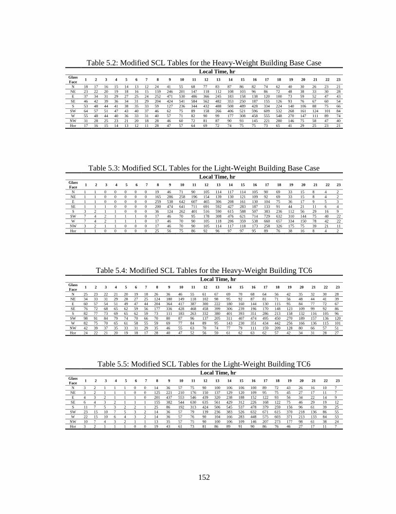
152
Table 5.2: Modified SCL Tables for the Heavy-Weight Building Base Case Local Time, hr Glass
Face 1 2 3 4 5 6 7 8 9 10 11 12 13 14 15 16 17 18 19 20 21 22 23 24
N 18 17 16 15 14 13 12 24 41 55 68 77 83 87 86 82 74 62 40 30 26 23 21 20
NE 23 22 20 19 18 16 15 159 246 201 147 118 112 108 103 96 86 72 48 38 33 30 28 25
E 37 34 31 29 27 25 24 252 471 530 486 366 245 183 158 138 120 100 73 59 52 47 43 40
SE 46 42 39 36 34 31 29 204 424 541 584 562 482 353 250 187 155 126 93 76 67 60 54 49
S 53 48 44 41 38 35 33 59 127 236 344 432 488 508 489 428 334 224 140 106 88 75 66 59
SW 64 57 51 47 43 40 37 46 62 75 89 158 266 406 521 596 609 532 268 161 124 101 84 72
W 55 48 44 40 36 33 31 40 57 71 82 90 99 177 308 458 555 548 270 147 111 89 74 63
NW 31 28 25 23 21 20 18 28 46 60 72 81 87 90 93 145 221 280 146 75 58 47 40 35
Hor 17 16 15 14 13 12 11 28 47 57 64 69 72 74 75 75 73 65 41 29 25 23 21 19
Table 5.3: Modified SCL Tables for the Light-Weight Building Base Case Local Time, hr Glass
Face 1 2 3 4 5 6 7 8 9 10 11 12 13 14 15 16 17 18 19 20 21 22 23 24
N 1 1 0 0 0 0 0 19 46 71 90 105 114 117 114 105 90 69 33 15 8 4 2 1
NE 1 1 0 0 0 0 0 165 286 258 196 154 139 130 121 109 92 69 33 15 8 4 2 1
E 1 1 0 0 0 0 0 259 538 642 607 465 306 208 161 130 104 75 36 17 9 5 3 2
SE 1 1 1 0 0 0 0 200 474 641 711 691 592 427 283 187 133 91 44 21 11 6 4 2
S 3 2 1 1 0 0 0 36 124 262 401 516 590 615 588 507 383 236 112 56 29 16 9 5
SW 7 4 2 1 1 1 0 17 46 70 95 178 308 476 621 714 729 632 310 144 75 40 22 12
W 7 4 2 1 1 1 0 17 46 70 90 105 118 206 359 538 660 657 334 150 78 42 22 12
NW 3 2 1 1 0 0 0 17 46 70 90 105 114 117 118 173 258 326 175 75 39 21 11 6
Hor 1 1 0 0 0 0 0 25 56 75 86 92 96 97 97 95 89 76 38 16 8 4 2 1
Table 5.4: Modified SCL Tables for the Heavy-Weight Building TC6 Local Time, hr Glass
Face 1 2 3 4 5 6 7 8 9 10 11 12 13 14 15 16 17 18 19 20 21 22 23 24
N 25 23 22 21 20 19 18 26 36 46 55 61 67 69 70 68 64 56 42 35 32 30 28 26
NE 34 33 31 29 28 27 25 124 180 149 118 102 98 95 92 87 81 71 56 48 44 41 39 36
E 60 57 54 51 49 47 44 204 364 417 387 300 222 180 160 144 130 115 95 84 77 72 67 63
SE 76 72 68 65 62 59 56 177 336 428 468 458 399 306 239 196 170 148 123 109 99 92 86 81
S 82 77 73 69 65 62 59 73 111 183 263 332 380 401 393 351 286 213 158 132 116 105 96 88
SW 98 91 84 79 74 70 66 70 80 87 96 137 205 311 407 474 495 450 270 189 157 136 120 108
W 82 75 70 65 61 58 55 59 69 77 84 89 95 143 230 351 434 442 256 166 136 115 101 90
NW 42 39 37 35 33 31 29 35 46 55 63 70 74 77 79 111 159 209 128 80 66 57 51 46
Hor 24 22 21 20 19 18 17 28 40 47 52 56 59 61 62 63 62 57 42 34 31 28 27 25
Table 5.5: Modified SCL Tables for the Light-Weight Building TC6 Local Time, hr Glass
Face 1 2 3 4 5 6 7 8 9 10 11 12 13 14 15 16 17 18 19 20 21 22 23 24
N 3 2 1 1 1 0 0 14 36 57 75 90 100 106 106 100 89 72 43 26 16 10 7 4
NE 3 2 1 1 1 0 0 125 221 210 176 150 137 129 120 109 95 75 45 27 17 11 7 5
E 4 3 2 1 1 1 0 201 437 553 546 439 320 238 188 152 122 93 56 34 22 14 9 6
SE 6 4 3 2 1 1 1 155 382 544 630 635 561 429 312 226 168 122 75 46 29 19 12 8
S 11 7 5 3 2 2 1 25 86 192 313 424 506 545 537 478 379 259 156 96 61 39 25 16
SW 23 15 10 7 5 3 2 14 36 57 79 139 236 383 526 632 671 615 370 218 136 86 55 35
W 22 15 10 6 4 3 2 14 36 57 76 90 104 166 283 448 575 603 371 213 133 84 53 34
NW 10 7 4 3 2 1 1 13 35 57 75 90 100 106 109 146 207 273 177 98 61 38 24 16
Hor 3 2 1 1 1 0 0 19 43 61 73 81 86 89 91 90 86 76 46 27 17 11 7 4

153
Table 5.6: Modified SCL Tables for the Heavy-Weight Building TC12 Local Time, hr Glass
Face 1 2 3 4 5 6 7 8 9 10 11 12 13 14 15 16 17 18 19 20 21 22 23 24
N 24 23 21 20 19 18 18 25 35 45 53 59 64 67 68 66 61 54 40 34 31 29 27 25
NE 33 31 30 28 27 26 24 120 170 137 110 96 93 91 88 83 77 68 53 46 42 39 37 35
E 58 55 52 50 47 45 43 201 359 409 375 283 211 173 154 139 125 111 92 81 74 69 65 61
SE 73 69 66 62 59 57 54 173 329 419 458 446 382 289 227 188 164 142 119 105 96 89 83 78
S 78 73 69 65 61 58 55 68 102 168 246 315 363 384 374 331 267 199 149 125 110 99 90 83
SW 95 88 82 76 72 68 64 68 77 84 92 129 189 295 394 461 483 439 262 184 153 131 116 104
W 79 73 68 63 59 56 53 57 67 75 81 87 92 134 215 339 423 433 250 162 132 112 98 88
NW 40 37 35 33 31 29 28 34 44 53 61 67 72 74 76 103 146 198 122 75 63 54 48 44
Hor 23 22 21 20 19 18 17 27 38 46 50 54 57 59 60 61 60 55 40 33 30 27 26 24
Table 5.7: Modified SCL Tables for the Light-Weight Building TC12 Local Time, hr Glass
Face 1 2 3 4 5 6 7 8 9 10 11 12 13 14 15 16 17 18 19 20 21 22 23 24
N 3 2 1 1 1 0 0 13 34 55 73 87 97 102 102 97 86 70 42 25 15 10 6 4
NE 3 2 1 1 1 0 0 121 210 194 164 141 130 123 115 105 91 73 43 26 16 10 7 4
E 4 3 2 1 1 1 0 199 431 543 530 417 304 227 180 146 117 89 54 33 21 14 9 6
SE 5 4 2 2 1 1 1 152 375 533 617 619 540 406 296 215 160 116 71 44 28 18 12 8
S 10 7 5 3 2 1 1 23 77 175 293 402 483 522 513 452 354 241 145 89 56 36 23 15
SW 23 15 10 7 4 3 2 13 35 55 76 130 217 362 507 614 655 601 361 212 133 84 54 35
W 22 14 9 6 4 3 2 13 35 55 73 87 100 156 264 431 560 591 364 209 130 82 52 34
NW 10 6 4 3 2 1 1 13 34 55 73 87 97 102 105 136 190 257 168 93 58 36 23 15
Hor 3 2 1 1 1 0 0 18 42 59 71 78 83 86 87 87 83 73 45 26 16 10 7 4
154
Figure 5.2 and Figure 5.3 show the comparisons of base-case sensible cooling load
predicted by the HBM, the RTSM, the CLTD/SCL/CLF Method and the modified
CLTD/SCL/CLF Method for both the heavy-weight (Figure 5.2) and light-weight
(Figure 5.3) building cases. The results showed the peak sensible cooling load for the
heavy-weight building using the original CLTD/SCL/CLF Method decreased from
5,976.3 W to 5,022.4 W by applying the updated SCL tables, which had a difference of -
15.96%. The peak cooling load using CLTD/SCL/CLF Method was decreased by 28%,
compared to HBM baseline. The peak sensible cooling load for the light-weight building
using the original CLTD/SCL/CLF Method decreased from 6,145.2 W to 6,049.4 W by
applying updated SCL tables, which had a difference of -1.56%. The peak cooling load
using CLTD/SCL/CLF Method was decreased by 3.5%, compared to HBM baseline.
Since the SCL tables were derived from the RTSM, the modified CLTD/SCL/CLF
Method brought the peak cooling load closer to the RTSM and HBM results, when
compared to the original CLTD/SCL/CLF Method. However, the profile still did not
exactly match by the RTSM profile. This is because the sensible cooling load profile was
driven by both CLTD and SCL tables. In the results shown, only the SCL tables were
updated and the CLTD tables remained unchanged.
For both the heavy-weight and light-weight building cases, the peak sensible cooling
load peaks from the different methods all occurred at 5:00 P.M., which indicated a good
alignment of peak time. During the morning and night time, the peak cooling load by the
modified CLTD/SCL/CLF Method was above the peak cooling load by the RTSM,
which appeared asymmetric pattern.
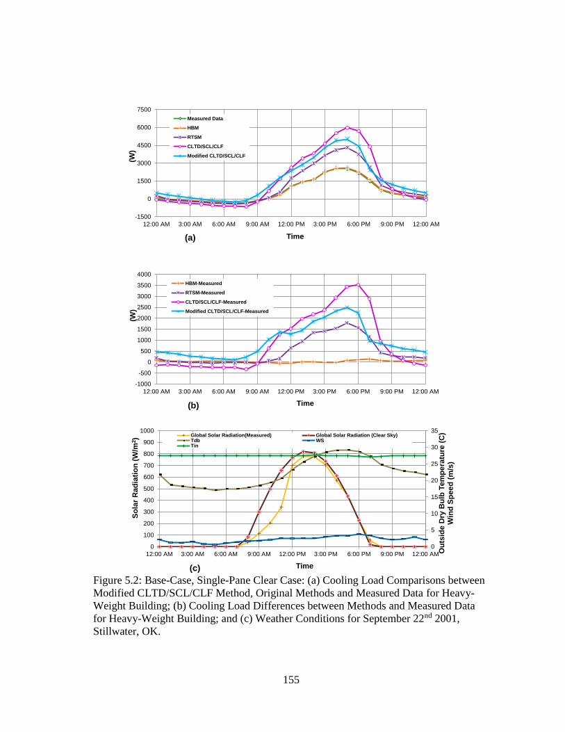
155
-1500
0
1500
3000
4500
6000
7500
12:00 AM 3:00 AM 6:00 AM 9:00 AM 12:00 PM 3:00 PM 6:00 PM 9:00 PM 12:00 AM
(W)
Time
Measured Data
HBM
RTSM
CLTD/SCL/CLF
Modified CLTD/SCL/CLF
-1000
-500
0
500
1000
1500
2000
2500
3000
3500
4000
12:00 AM 3:00 AM 6:00 AM 9:00 AM 12:00 PM 3:00 PM 6:00 PM 9:00 PM 12:00 AM
(W)
Time
HBM-Measured
RTSM-Measured
CLTD/SCL/CLF-Measured
Modified CLTD/SCL/CLF-Measured
(b)(b)(b)(b)(b)
(a)
0
5
10
15
20
25
30
35
0
100
200
300
400
500
600
700
800
900
1000
12:00 AM 3:00 AM 6:00 AM 9:00 AM 12:00 PM 3:00 PM 6:00 PM 9:00 PM 12:00 AM Ou
tsid
e D
ry B
ulb
Te
mp
era
ture
(C
)W
ind
Sp
ee
d (
m/s
)
So
lar
Ra
dia
tio
n (
W/m
2)
Time
Global Solar Radiation(Measured) Global Solar Radiation (Clear Sky)Tdb WSTin
(c) Figure 5.2: Base-Case, Single-Pane Clear Case: (a) Cooling Load Comparisons between
Modified CLTD/SCL/CLF Method, Original Methods and Measured Data for Heavy-
Weight Building; (b) Cooling Load Differences between Methods and Measured Data
for Heavy-Weight Building; and (c) Weather Conditions for September 22nd 2001,
Stillwater, OK.

156
-1500
0
1500
3000
4500
6000
7500
12:00 AM 3:00 AM 6:00 AM 9:00 AM 12:00 PM 3:00 PM 6:00 PM 9:00 PM 12:00 AM
(W)
Time
Measured Data
HBM
RTSM
CLTD/SCL/CLF
Modified CLTD/SCL/CLF
(a)
-1000
-500
0
500
1000
1500
2000
2500
3000
3500
4000
12:00 AM 3:00 AM 6:00 AM 9:00 AM 12:00 PM 3:00 PM 6:00 PM 9:00 PM 12:00 AM
(W)
Time
HBM-Measured
RTSM-Measured
CLTD/SCL/CLF-Measured
Modified CLTD/SCL/CLF-Measured
(b)(b)(b)(b)(b)
0
5
10
15
20
25
30
35
0
100
200
300
400
500
600
700
800
900
1000
12:00 AM 3:00 AM 6:00 AM 9:00 AM 12:00 PM 3:00 PM 6:00 PM 9:00 PM 12:00 AM Ou
tsid
e D
ry B
ulb
Te
mp
era
ture
(C
)W
ind
Sp
ee
d (
m/s
)
So
lar
Ra
dia
tio
n (
W/m
2)
Time
Global Solar Radiation(Measured) Global Solar Radiation (Clear Sky)Tdb WSTin
(c) Figure 5.3: Base-Case, Single-Pane Clear Case: (a) Cooling Load Comparisons between
Modified CLTD/SCL/CLF Method, Original Methods and Measured Data for Light-
Weight Building; (b) Cooling Load Differences between Methods and Measured Data
for Light-Weight Building; and (c) Weather Conditions for September 22nd 2001,
Stillwater, OK.
157
Figure 5.4 and Figure 5.5 show the comparisons of TC6 test case sensible cooling
load predicted by the HBM, the RTSM, the CLTD/SCL/CLF Method and the modified
CLTD/SCL/CLF Method for both the heavy-weight (Figure 5.4) and light-weight
(Figure 5.5) building cases. The results showed the peak sensible cooling load for the
heavy-weight building using the original CLTD/SCL/CLF Method decreased from
4,597.2 W to 3,145.5 W using the updated SCL tables, which had a difference of -
31.58%. The peak cooling load using CLTD/SCL/CLF Method was decreased by 64%,
compared to HBM baseline. The peak sensible cooling load for light-weight building
using the original CLTD/SCL/CLF Method decreased from 4,771.1 W to 4,310.1 W
using the updated SCL tables, which had a difference of -9.66%. The peak cooling load
using CLTD/SCL/CLF Method was decreased by 28%, compared to HBM baseline. The
peak sensible cooling load profile using the modified CLTD/SCL/CLF Method in the
TC6 test case (i.e., double-pane clear glazing) matched more closely with the RTSM
profile, compared to the base case (i.e., single-pane clear glazing). The peak sensible
cooling load using the modified CLTD/SCL/CLF Method for the heavy-weight building
case in the TC6 test case was decreased more than the peak of the light-building case,
which had similar observation as the base case. The asymmetric pattern was also
improved for the double-pane clear versus the single-pane clear.
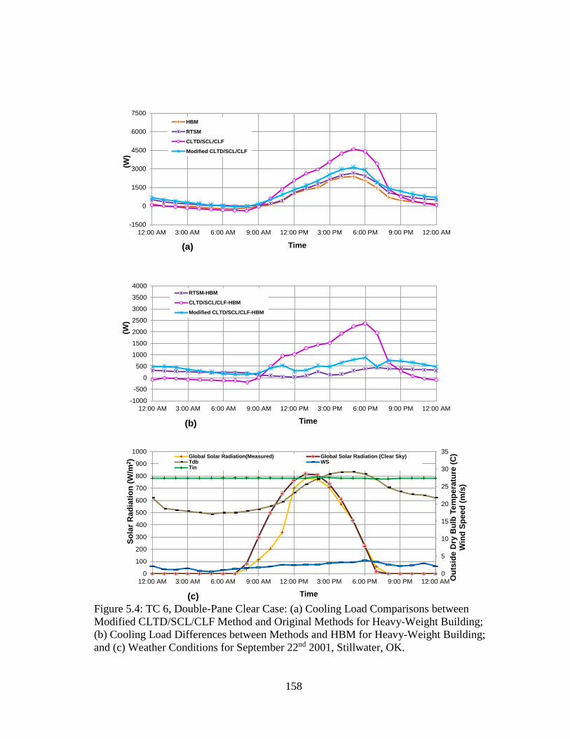
158
-1500
0
1500
3000
4500
6000
7500
12:00 AM 3:00 AM 6:00 AM 9:00 AM 12:00 PM 3:00 PM 6:00 PM 9:00 PM 12:00 AM
(W)
Time
HBM
RTSM
CLTD/SCL/CLF
Modified CLTD/SCL/CLF
-1000
-500
0
500
1000
1500
2000
2500
3000
3500
4000
12:00 AM 3:00 AM 6:00 AM 9:00 AM 12:00 PM 3:00 PM 6:00 PM 9:00 PM 12:00 AM
(W)
Time
RTSM-HBM
CLTD/SCL/CLF-HBM
Modified CLTD/SCL/CLF-HBM
(b)(b)(b)(b)(b)
0
5
10
15
20
25
30
35
0
100
200
300
400
500
600
700
800
900
1000
12:00 AM 3:00 AM 6:00 AM 9:00 AM 12:00 PM 3:00 PM 6:00 PM 9:00 PM 12:00 AM Ou
tsid
e D
ry B
ulb
Te
mp
era
ture
(C
)W
ind
Sp
ee
d (
m/s
)
So
lar
Ra
dia
tio
n (
W/m
2)
Time
Global Solar Radiation(Measured) Global Solar Radiation (Clear Sky)Tdb WSTin
(c)
(a)
Figure 5.4: TC 6, Double-Pane Clear Case: (a) Cooling Load Comparisons between
Modified CLTD/SCL/CLF Method and Original Methods for Heavy-Weight Building;
(b) Cooling Load Differences between Methods and HBM for Heavy-Weight Building;
and (c) Weather Conditions for September 22nd 2001, Stillwater, OK.

159
-1500
0
1500
3000
4500
6000
7500
12:00 AM 3:00 AM 6:00 AM 9:00 AM 12:00 PM 3:00 PM 6:00 PM 9:00 PM 12:00 AM
(W)
Time
HBM
RTSM
CLTD/SCL/CLF
Modified CLTD/SCL/CLF
(a)
-1000
-500
0
500
1000
1500
2000
2500
3000
3500
4000
12:00 AM 3:00 AM 6:00 AM 9:00 AM 12:00 PM 3:00 PM 6:00 PM 9:00 PM 12:00 AM
(W)
Time
RTSM-HBM
CLTD/SCL/CLF-HBM
Modified CLTD/SCL/CLF-HBM
(b)(b)(b)(b)(b)
0
5
10
15
20
25
30
35
0
100
200
300
400
500
600
700
800
900
1000
12:00 AM 3:00 AM 6:00 AM 9:00 AM 12:00 PM 3:00 PM 6:00 PM 9:00 PM 12:00 AM Ou
tsid
e D
ry B
ulb
Te
mp
era
ture
(C
)W
ind
Sp
ee
d (
m/s
)
So
lar
Rad
iati
on
(W
/m2)
Time
Global Solar Radiation(Measured) Global Solar Radiation (Clear Sky)Tdb WSTin
(c)
Figure 5.5: TC 6, Double-Pane Clear Case: (a) Cooling Load Comparisons between
Modified CLTD/SCL/CLF Method and Original Methods for Light-Weight Building;
(b) Cooling Load Differences between Methods and HBM for Light-Weight Building;
and (c) Weather Conditions for September 22nd 2001, Stillwater, OK.
160
Figure 5.6 and Figure 5.7 show the comparisons of TC12 test case sensible cooling
load predicted by the HBM, the RTSM, the CLTD/SCL/CLF Method and the modified
CLTD/SCL/CLF Method for both the heavy-weight and light-weight building cases. The
peak sensible cooling for the heavy-weight building using the original CLTD/SCL/CLF
Method decreased from 4,127.2 W to 2,707.1 W using the updated SCL tables, which
had a difference of -34.41%. The peak cooling load using CLTD/SCL/CLF Method was
decreased by 75%, compared to HBM baseline. The peak sensible cooling load for the
light-weight building using the original CLTD/SCL/CLF Method decreased from
4,301.4 W to 3,729.8 W using the updated SCL tables, which had a difference of -
13.29%. The peak cooling load using CLTD/SCL/CLF Method was decreased by 41%,
compared to HBM baseline. The peak sensible cooling load profile using the modified
CLTD/SCL/CLF Method in the TC12 test case (i.e., triple-pane clear glazing) more
closely matched the RTSM profile, compared to the base case (i.e., single-pane clear
glazing) and TC6 test case (i.e., double-pane clear glazing). The asymmetric pattern was
also improved for the triple-pane clear when compared to the double-pane clear glazing.

161
-1500
0
1500
3000
4500
6000
7500
12:00 AM 3:00 AM 6:00 AM 9:00 AM 12:00 PM 3:00 PM 6:00 PM 9:00 PM 12:00 AM
(W)
Time
HBM
RTSM
CLTD/SCL/CLF
Modified CLTD/SCL/CLF
-1000
-500
0
500
1000
1500
2000
2500
3000
3500
4000
12:00 AM 3:00 AM 6:00 AM 9:00 AM 12:00 PM 3:00 PM 6:00 PM 9:00 PM 12:00 AM
(W)
Time
RTSM-HBM
CLTD/SCL/CLF-HBM
Modified CLTD/SCL/CLF-HBM
(b)(b)(b)(b)(b)
0
5
10
15
20
25
30
35
0
100
200
300
400
500
600
700
800
900
1000
12:00 AM 3:00 AM 6:00 AM 9:00 AM 12:00 PM 3:00 PM 6:00 PM 9:00 PM 12:00 AM Ou
tsid
e D
ry B
ulb
Te
mp
era
ture
(C
)W
ind
Sp
ee
d (
m/s
)
So
lar
Rad
iati
on
(W
/m2)
Time
Global Solar Radiation(Measured) Global Solar Radiation (Clear Sky)Tdb WSTin
(c)
(a)
Figure 5.6: TC 12, Triple-Pane Clear Case: (a) Cooling Load Comparisons between
Modified CLTD/SCL/CLF Method and Original Methods for Heavy-Weight Building;
(b) Cooling Load Differences between Methods and HBM for Heavy-Weight Building;
and (c) Weather Conditions for September 22nd 2001, Stillwater, OK.

162
-1500
0
1500
3000
4500
6000
7500
12:00 AM 3:00 AM 6:00 AM 9:00 AM 12:00 PM 3:00 PM 6:00 PM 9:00 PM 12:00 AM
(W)
Time
HBM
RTSM
CLTD/SCL/CLF
Modified CLTD/SCL/CLF
(a)
-1000
-500
0
500
1000
1500
2000
2500
3000
3500
4000
12:00 AM 3:00 AM 6:00 AM 9:00 AM 12:00 PM 3:00 PM 6:00 PM 9:00 PM 12:00 AM
(W)
Time
RTSM-HBM
CLTD/SCL/CLF-HBM
Modified CLTD/SCL/CLF-HBM
(b)(b)(b)(b)(b)
0
5
10
15
20
25
30
35
0
100
200
300
400
500
600
700
800
900
1000
12:00 AM 3:00 AM 6:00 AM 9:00 AM 12:00 PM 3:00 PM 6:00 PM 9:00 PM 12:00 AM Ou
tsid
e D
ry B
ulb
Te
mp
era
ture
(C
)W
ind
Sp
ee
d (
m/s
)
So
lar
Rad
iati
on
(W
/m2)
Time
Global Solar Radiation(Measured) Global Solar Radiation (Clear Sky)Tdb WSTin
(c) Figure 5.7: TC 12, Triple-Pane Clear Case: (a) Cooling Load Comparisons between
Modified CLTD/SCL/CLF Method and Original Methods for Light-Weight Building;
(b) Cooling Load Differences between Methods and HBM for Light-Weight Building;
and (c) Weather Conditions for September 22nd 2001, Stillwater, OK.

163
5.3 Summary
This section presented a proposed procedure to update the SCL tables that were used
in the CLTD/SCL/CLF Method using the most recent fenestration heat gain calculation
model. Specifically, this model replaced the SC with an incidence angle-based SHGC.
The shading device influence can be further adjusted by indoor solar attenuation
coefficient (IAC). This new procedure was motivated by both the survey and interview
results as well as the discoveries made during the method comparisons shown in Chapter
IV.
Three test cases were chosen for this study to generally show results of the sensible
peak cooling loads estimated by the modified CLTD/SCL/CLF Method. All the results
showed decreased peak sensible cooling load using the updated SCL tables in the
modified CLTD/SCL/CLF Method, which brought the calculated peak closer to the
HBM results. One reason for this is that the new SCL tables were derived from the
ASHRAE RTSM Spreadsheet Tool. Therefore, the majority of the sensible cooling load
profiles followed the similar pattern of the RTSM profiles.
164
CHAPTER VI
RESULT SUMMARY, CONCLUSIONS AND FUTURE WORK
6.1 Result Summary and Conclusions
This dissertation has analyzed peak sensible cooling load calculation methods for
commercial building design in the U.S., including all cooling loads methods that have
been published in the 1967-2013 ASHRAE Handbook of Fundamentals.
The major contributions of this work are as follows:
1) A survey and phone interview of selected HVAC design professionals who
specialized in HVAC system design and load calculations.
2) A comprehensive analysis and comparison of five sensible peak cooling load
calculation methods, which are: the Heat Balance Method (HBM); the Radiant Time
Series Method (RTSM); the Transfer Function Method (TFM); the Total Equivalent
Temperature Difference/Time Averaging (TETD/TA) Method; and the Cooling Load
Temperature Difference/Solar Cooling Load/Cooling Load Factor (CLTD/SCL/CLF)
Method. The comparison analysis was presented in two parts. The first part focused on
an analysis and the comparison of five methods against measured data from the RP-1117
report. The second part of the analysis was additional case-study analysis that compared
the four methods against the HBM varying the window parameters (i.e., the window area
and glazing properties).
165
3) Finally, a proposed analysis that updates the SCL tables used in the
CLTD/SCL/CLF Method was performed and a method provided to integrate the most
recent fenestration heat gain model by using SHGC.
6.1.1 Results from the Survey and Phone Interview Study
Both a one-page survey and a fifteen-minute phone interview were conducted with
the selected participants. The following findings were obtained:
All peak load calculation methods are still available for engineers to use.
The majority of the engineers interviewed used the CLTD/SCL/CLF Method.
Most people who used this method used the TRACE 700 software.
The second most popular method used by the participants was the TETD/TA
Method, the RTSM, followed by the HBM. None of the participants are using the TFM,
even though some were familiar to the TFM principles.
Several participants said the HBM was the most accurate method, although it
had drawbacks of being complex and lacked a breakdown of cooling load component
output.
With the exception of LEED design requirements, the RTSM was rarely in use
since other simplified methods were easier-to-use and had acceptable accuracy.
All the current methods were deemed to be good enough for designing today’s
commercial buildings. In some instances, the inputs for the software need to be better
managed.
166
6.1.2 Results from the Analysis and Comparison of the Peak Cooling Load Design
Methods
In the first part of the analysis, the data from the ASHRAE RP-1117 report were
used as a comparison for the peak cooling design load methods. In this analysis, the
building configurations and construction materials remained unchanged. The sensible
cooling load analysis from the TFM, the TETD/TA Method, and the CLTD/SCL/CLF
Method were analyzed along with the calculation that represented the HBM and the
RTSM. This analysis showed the following:
Differences in the published ASHRAE clear-sky models. Two clear-sky models
were published by ASHRAE from 1967 to 2013, which were the 1967 ASHRAE clear-
sky model and the 2009 ASHRAE clear-sky model. In the 1967 ASHRAE clear-sky
model, two sets of A, B, C coefficients were published in the ASHRAE Handbook. One
set was in the 1967-2001 ASHRAE Handbook of Fundamentals and the other set was in
the 2005 ASHRAE Handbook of Fundamentals. The 2009 ASHRAE clear-sky model
calculates a larger beam solar radiation component compared to the 1967 ASHRAE
clear-sky model. In addition, the diffuse solar radiation from the 2009 ASHRAE clear-
sky model falls between the values predicted by the 1967 ASHRAE clear-sky model
using the two sets of A, B, C coefficients. The total solar radiation calculated by the
2009 ASHRAE clear-sky model is the largest among all methods. Finally, no case
studies were found that fully compared the ASHRAE clear-sky models. Even in the
2009 and 2013 ASHRAE Handbook of Fundamentals different coefficients were
presented to calculate air mass components, without explanation. Therefore, before

167
calculating a peak cooling load, the choice of clear-sky model should be carefully
reviewed to avoid any unexpected results.
Differences in FORTRAN source code. The FORTRAN source codes published
in the ASHRAE LOADS Toolkit CD does not allow the reader to replicate the results
published in RP-1117 report. This was resolved by contacting the authors of this project.
Limitations in the HB LOADS Toolkit Output. The sensible peak cooling load
produced by the HB LOADS Toolkit did not provide a detailed breakdown of each
component that was contributing to the total cooling load. Unfortunately, in order to
obtain a detailed output, the source code needed to be modified and recompiled.
Replication of the RP-1117 results could not be performed with the ASHRAE
RTSM Spreadsheet Tool. Instead of using the RTSM LOADS Toolkit to estimate the
sensible peak cooling load, the 2009 ASHRAE RTSM Spreadsheet Tool was selected to
perform the analysis. Unfortunately, the RP-1117 results could not be exactly replicated.
The reason remains unknown because the simulation files that were used by RP-1117
could not be obtained. Nevertheless, the over-prediction issues reported by RP-1117
were also found in this study for cases with a large single-pane clear glazing. Compared
to the measured data, the RTSM over-predicted the cooling load for both the heavy-
weight and light-weight building cases, which were 68.32 % and 57.83% differences,
respectively.
The TFM over-predicted the peak cooling load. To apply the TFM principles to
the base case, the proper wall and roof group was selected and the fenestration heat gain
model used SHGC instead of SC. Compared to the measured data, the TFM over-
168
predicted the cooling load for both the heavy-weight and light-weight building cases,
which were 77.64 % and 57.17% differences, respectively.
The TETD/TA Method required subjective input and over-predicted the cooling
load. The TETD/TA Method tends to be subjective since the designer needs to pick a
period for the time-averaging process, which can vary from one person to the next. In the
analysis, the fenestration heat gain model used SHGC analysis. Compared to the
measured data, the TETD/TA over-predicted the cooling load for both the heavy-weight
and light-weight building cases, which were 114.73% and 69.34% different,
respectively.
It was difficult to modify the CLTD/SCL/CLF Method for use with measured
solar data. The CLTD/SCL/CLF Method was designed as a manual method. By directly
applying the equations, the sensible cooling load can be achieved in one step.
Unfortunately, many assumptions are required to generate the CLTD, SCL, and CLF
tables. For example, the 1967 ASHRAE clear-sky model was used to generate the
original published tables. In addition, the SC was used in the fenestration heat gain
calculations. Therefore, there was little room to apply measured solar data and SHGC
fenestration heat gain model. Nevertheless, the CLTD/SCL/CLF Method over-predicted
the peak cooling load for both the heavy-weight and light-weight building cases, which
were 132.31% and 80.05%, respectively.
The most accurate cooling load calculation was the HBM, followed by the
RTSM, the TFM, the TETD/TA Method, and the CLTD/SCL/CLF Method. The sensible
cooling load comparisons of the HBM, the RTSM, the TFM, the TETD/TA Method, and

169
the CLTD/SCL/CLF Method were analyzed. In general, all simplified methods tended to
over-predict the peak cooling load. The RTSM and TFM showed the close peak cooling
load estimation. The comparison between RTSM and TFM showed differences to be
5.54% and -0.42% for the heavy-weight and light-weight buildings, respectively.
Compared to the measured data, the HBM provided the most accurate peak prediction,
followed by the RTSM, the TFM and the TETD/TA Method. The less accurate method
was proved to be CLTD/SCL/CLF Method.
In the second part of the analysis, additional peak cooling loads were analyzed to
further understand the impact of window area and glazing types on the sensible cooling
load by applying the HBM, the RTSM, the TFM, the TETD/TA Method, and the
CLTD/SCL/CLF Method. To perform this comparison, the HBM was treated as the
baseline and other methods compared with it. Fifteen cases were prepared for this
second comparison analysis. The following conclusions were obtained during this
second analysis:
All the cases with a 5% WWR tended to under-estimate the peak cooling loads
compared to the HBM. For the heavy-weight building, the RTSM under-estimated the
cooling load the most, while, for light-weight building, the TFM underestimated the
cooling load the most, other than the RTSM.
For the remainder of the test cases, the simplified methods tended to over-
estimate the sensible peak cooling load. The results from the RTSM and the TFM were
fairly close. The worst prediction was still the CLTD/SCL/CLF Method.

170
The RTSM for test case 12 provided the best estimation of sensible cooling load
for all heavy-weight building case simulations. Across all types of window glazing, the
cooling load of the test case 12 with a 25% WWR and triple pane clear windows by the
RTSM was 0.83% percentage difference compared to the HBM, which was considered
the best match between the RTSM and HBM for all heavy-weight building case
simulation.
The RTSM for test case 5 provided the best estimation of sensible peak cooling
load for all light-weight building case simulations, followed by the TFM. Across all
types of window glazing, the cooling load of the test case 5 with 15% WWR and double
pane clear windows by the TFM and the RTSM was -1.09% and -1.85% percentage
difference, respectively, compared to the HBM, which were considered the best and the
second best peak cooling load estimations for all light-weight building case simulation.
The most accurate simplified peak cooling load calculation method was the
RTSM, followed by the TFM, the TETD/TA Method, and the CLTD/SCL/CLF Method.
For most test cases, the RTSM worked fairly well. The second most accurate method
was the TFM. The least accurate method was the CLTD/SCL/CLF method. The
TETD/TA Method results were in between the TFM and the CLTD/SCL/CLF Method.
This was consistent with the base case results.
The simplified methods were more sensitive to the glazing area and glazing type.
The RTSM, the TFM, the TETD/TA Method and the CLTD/SCL/CLF Method were
very sensitive to the glazing area and glazing type. In contrast, the HBM was very steady
171
and predicted the cooling load reasonably over a range of test cases. For all methods, the
use of better SHGC lowered the peak cooling load.
6.1.3 Results from the Proposed Analysis to Update the SCL Tables for
CLTD/SCL/CLF Method Using ASHRAE RTSM Spreadsheet Tool
An attempt to update SCL tables in the CLTD/SCL/CLF Method was made by using
the ASHRAE RTSM Spreadsheet Tool. The purpose of this was to update the
fenestration heat gain model by using an angular-based SHGC, rather than the SC. Based
on this analysis, the following conclusions were obtained:
It is possible to re-define the SCL by deriving it from a more accurate
fenestration heat gain model. The previous SCL tables were based on the SC, the Double
Strength (DSA) Glass coefficients and the TFM calculations. Since the comparisons
showed the RTSM performed better than the TFM, the new sets of tables were based on
the RTSM principles to update fenestration heat gain model.
Three selected examples showed a decreased cooling load peak using the updated,
modified SCL tables. In all cases, the peak cooling load was closer to the RTSM and
HBM results.
As glazing was varied from single-pane clear to double and triple-pane clear, the
peak cooling load profile using modified SCL tables showed a more accurate profile
compared to the RTSM and decreased peak load.
172
6.2 Future Work
The following work needs to be performed in the future:
ASHRAE should confirm the survey results in this study with additional
interviews of field professionals throughout the U.S. who use peak load calculations.
The 2009 ASHRAE clear-sky model needs to be further analyzed to assure its
accuracy.
All peak cooling load methods should be updated with the most recent 2009
ASHRAE clear-sky model.
ASHRAE should reconsider updating the CLTD/SCL/CLF Method for both
architects and engineers to use and publishing the newly updated method in an ASHRAE
special publication.
The CLTD and CLF tables should be updated using the 2006 spreadsheet tool
proposed by TC 4.1 volunteers and the results published in an ASHRAE special
publication.
The SCL tables should be updated following the proposed methodology.
The ETD tabulated tables can be updated based on the TETD/TA Method with
an updated fenestration heat gain model.
The HBM should be further analyzed to provide a detailed cooling load
component output to facilitate the comparison;
Additional experiments should be set up to further study the comparison of all
methods.

173
REFERENCES
Acott, C. 1999. A Brief History of Diving and Decompression Illness. Journal of South
Pacific Underwater Medicine Society, 29(2), 98-109.
Allen, J.R., Walker, J.H., and Giesecke, F.E. 1931. Heating and Ventilation. New York,
NY and London: McGraw-Hill Book Company.
Alford, J.S., Ryan, J.E., and Urban, F.O. 1939. Effect of Heat Storage and Variation in
Outdoor Temperature and Solar Intensity on Heat Transfer through Walls. ASHVE
Transactions, 45, 369-380.
Al-Rabghi, O.M.A. and Al-Johani, K.M. 1997. Utilizing Transfer Function Method for
Hourly Cooling Load Calculations. Energy Convers, Mgmt, Vol.38, No. 4, 319-332.
Anonymous. 1997. Timeline: 50 Years of Computing. T.H.E. Journal, 24(11), 32.
Archibald, T., Fraser, C., and Grattan-Guinness, I. 2004. The History of Differential
Equations, 1670-1950. Mathematisches Forschungsinstitut Oberwolfach Report No.
51/2004.
Arens, E.A. 1977. Geographic Variation in the Heating and Cooling Requirements of A
Typical Single Family House and Correction of This Requirement to Degree Days.
NBSIR National Bureau of Standards Report Building Science Series 116.
ASHRAE. 1961. Chapters 23, 25 and 26. ASHRAE Guide and Data Book 1961:
Fundamentals and Equipment. New York: American Society of Heating,
Refrigerating and Air-Conditioning Engineers, Inc.
ASHRAE. 1963. Chapters 23, 25 and 26. ASHRAE Guide and Data Book 1963:
Fundamentals and Equipment. New York: American Society of Heating,
Refrigerating and Air-Conditioning Engineers, Inc.
ASHRAE. 1965. Chapters 24, 26 and 27. ASHRAE Guide and Data Book :
Fundamentals and Equipment for 1965 and 1966. New York: American Society of
Heating, Refrigerating and Air-Conditioning Engineers, Inc.
ASHRAE. 1967. Chapters 26, 27 and 28. ASHRAE Handbook of Fundamentals. Atlanta,
GA: American Society of Heating, Refrigerating and Air-Conditioning Engineers,
Inc.
ASHRAE. 1972. Chapters 20, 21 and 22. ASHRAE Handbook of Fundamentals. Atlanta,
GA: American Society of Heating, Refrigerating and Air-Conditioning Engineers,
Inc.
174
ASHRAE. 1977. Chapters 22, 24 and 25. ASHRAE Handbook of Fundamentals. Atlanta,
GA: American Society of Heating, Refrigerating and Air-Conditioning Engineers,
Inc.
ASHRAE. 1981. Chapters 25, 26 and 28. ASHRAE Handbook of Fundamentals. Atlanta,
GA: American Society of Heating, Refrigerating and Air-Conditioning Engineers,
Inc.
ASHRAE. 1985. Chapters 25, 26 and 28. ASHRAE Handbook of Fundamentals. Atlanta,
GA: American Society of Heating, Refrigerating and Air-Conditioning Engineers,
Inc.
ASHRAE. 1989. Chapters 25, 26 and 28. ASHRAE Handbook of Fundamentals. Atlanta,
GA: American Society of Heating, Refrigerating and Air-Conditioning Engineers,
Inc.
ASHRAE. 1993. Chapters 25, 26 and 28. ASHRAE Handbook of Fundamentals. Atlanta,
GA: American Society of Heating, Refrigerating and Air-Conditioning Engineers,
Inc.
ASHRAE. 1997. Chapters 27, 28 and 30. ASHRAE Handbook of Fundamentals. Atlanta,
GA: American Society of Heating, Refrigerating and Air-Conditioning Engineers,
Inc.
ASHRAE. 2001. Chapters 28, 29 and 31. ASHRAE Handbook of Fundamentals. Atlanta,
GA: American Society of Heating, Refrigerating and Air-Conditioning Engineers,
Inc.
ASHRAE. 2004. Advanced Energy Design Guide for Small Office Buildings: Achieving
30% Energy Savings toward a Net Zero Energy Building. Atlanta, GA: American
Society of Heating, Refrigerating and Air-Conditioning Engineers, Inc.
ASHRAE. 2005. Chapters 29, 30 and 32. ASHRAE Handbook of Fundamentals. Atlanta,
GA: American Society of Heating, Refrigerating and Air-Conditioning Engineers,
Inc.
ASHRAE. 2008a. Advanced Energy Design Guide for Small Warehouses and Self-
Storage Buildings: Achieving 30% Energy Savings toward a Net Zero Energy
Building. Atlanta, GA: American Society of Heating, Refrigerating and Air-
Conditioning Engineers, Inc.

175
ASHRAE. 2008b. Advanced Energy Design Guide for K-12 School Buildings:
Achieving 30% Energy Savings toward a Net Zero Energy Building. Atlanta, GA:
American Society of Heating, Refrigerating and Air-Conditioning Engineers, Inc.
ASHRAE. 2008c. Advanced Energy Design Guide for Small Retail Buildings: Achieving
30% Energy Savings toward a Net Zero Energy Building. Atlanta, GA: American
Society of Heating, Refrigerating and Air-Conditioning Engineers, Inc.
ASHRAE. 2009a. Advanced Energy Design Guide for Small Hospitals and Healthcare
Facilities: Achieving 30% Energy Savings toward a Net Zero Energy Building.
Atlanta, GA: American Society of Heating, Refrigerating and Air-Conditioning
Engineers, Inc.
ASHRAE. 2009b. Advanced Energy Design Guide for Highway Lodging: Achieving
30% Energy Savings toward a Net Zero Energy Building. Atlanta, GA: American
Society of Heating, Refrigerating and Air-Conditioning Engineers, Inc.
ASHRAE. 2009c. Chapter s17, 18 and 19. ASHRAE Handbook of Fundamentals.
Atlanta, GA: American Society of Heating, Refrigerating and Air-Conditioning
Engineers, Inc.
ASHRAE. 2009d. Updating the ASHRAE Climate Data for Design and Standards.
ASHRAE Research Project Report RP-1453.
ASHRAE. 2010. ANSI/ASHRAE Standard 90.1-2010: Energy Standard for Buildings
Except Low-Rise Residential Buildings. Atlanta, GA: American Society of Heating,
Refrigerating and Air-Conditioning Engineers, Inc.
ASHRAE. 2011a. ANSI/ASHRAE/USGBC/IES Standard 189.1-2011. Atlanta, GA:
American Society of Heating, Refrigerating and Air-Conditioning Engineers, Inc.
ASHRAE. 2011b. Advanced Energy Design Guide for K-12 School Buildings:
Achieving 50% Energy Savings toward a Net Zero Energy Building. Atlanta, GA:
American Society of Heating, Refrigerating and Air-Conditioning Engineers, Inc.
ASHRAE. 2011c. Advanced Energy Design Guide for Small to Medium Office
Buildings: Achieving 50% Energy Savings toward a Net Zero Energy Building.
Atlanta, GA: American Society of Heating, Refrigerating and Air-Conditioning
Engineers, Inc.
ASHRAE. 2011d. Advanced Energy Design Guide for Medium to Bid Box Retail
Buildings: Achieving 50% Energy Savings toward a Net Zero Energy Building.
Atlanta, GA: American Society of Heating, Refrigerating and Air-Conditioning
Engineers, Inc.
176
ASHRAE. 2012. Advanced Energy Design Guide for large Hospitals: Achieving 50%
Energy Savings toward a Net Zero Energy Building. Atlanta, GA: American Society
of Heating, Refrigerating and Air-Conditioning Engineers, Inc.
ASHRAE. 2013a. ASHRAE Handbook of Fundamentals. Atlanta, GA: American
Society of Heating, Refrigerating and Air-Conditioning Engineers, Inc.
ASHRAE. 2013b. ANSI/ASHRAE Standard 90.1-2013: Energy Standard for Buildings
Except Low-Rise Residential Buildings. Atlanta, GA: American Society of Heating,
Refrigerating and Air-Conditioning Engineers, Inc.
ASHRAE. 2014. ANSI/ASHRAE/USGBC/IES Standard 189.1-2014. Atlanta, GA:
American Society of Heating, Refrigerating and Air-Conditioning Engineers, Inc.
ASME. 1991. The Milam Building, San Antonio, Texas: A National Mechanical
Engineering Heritage Site. New York: ASME Book No. HH9106. Retrieved May,
2012, from:
https://www.asme.org/getmedia/b0ab0ff1-c44b-45af-97a5-fb5f53e80630/155-
Milam-High-rise-Air-Conditioned-Building.aspx
ASHVE. 1922. American Society of Heating and Ventilating Engineers Guide. New
York: American Society of Heating and Ventilating Engineers.
ASHVE. 1951. American Society of Heating and Ventilating Engineers Guide. New
York: American Society of Heating and Ventilating Engineers.
APEC. 1967. HCC-Heating/Cooling Load Calculation Program. Dayton, OH:
Automated Procedures for Engineering Consultants, Inc.
Ayres, J.M. and Stamper, E. 1995. Historical Development of Building Energy
Calculations. ASHRAE Transactions, 101, Pt.1, 841-849.
Backman, D., and Harman, P. 2011. NASA: Inquiry Activities for Learning about Light,
the EM Spectrum, and Multi-Wavelength Astronomy. Retrieved June 18, 2012, from
http://www.sofia.usra.edu/Edu/materials/2011DecNSTA_EMspectrum_MultiwaveA
stro.pdf
Buchberg, H. 1955. Electric Analogue Prediction of the Thermal Behavior of an
Inhabitable Enclosure. ASHAE Transactions, 61, 177.
Buchberg, H. 1958. Cooling Load from Thermal Network Solutions. ASHRAE
Transactions, 64, 111-128.

177
Box, G.E.P., and Jenkins, G.M. 1976. Time Series Analysis: Forecasting and Control.
Oakland, CA: Holden-Day, Inc.
Barnaby, C.S., Spilter, J.D., and Xiao, D. 2004. Updating the ASHRAE/ACCA
Residential Heating and Cooling Load Calculation Procedures and Data. ASHRAE
Final Report 1199, Atlanta, GA: American Society of Heating, Refrigerating and
Air-Conditioning Engineers, Inc.
Bergles, A.E. 1988. Enhancement of Convective Heat Transfer: Newton’s Legacy
Pursued. History of Heat Transfer, eds. Layton, E.T., Jr. & Lienhard, J.H., New York,
53-64.
Brisken, W.R. and Reque, S.G. 1956. Heat Load Calculations by Thermal Response.
ASHRAE Transactions, 62, 391-424.
Bruning, S.F. 2012. Load Calculation Spreadsheets: Quick Answers without Relying on
Rules of Thumb. ASHRAE Journal, 54(1), 40-46.
Bruning, S.F. 2016. Private Communication: Three files delivered by email on January
27.
Carrier, W.H. 1911. Rational Psychrometric Formulae. ASME Transactions, 33, 1005-
1053.
Clyde, G.D. 1931. Snow-Melting Characteristics. Utah Experiment Station Bulletin
No.231, Utah State Agricultural College.
Clough, R.W. 1960. The Finite Element Method in Plane Stress Analysis. Proceedings
of Second ASCE Conference on Electronic Computation, Pittsburg, Pennsylvania, 8,
345-378.
Crawley, D.B., Lawrie, L.K., Winkelmann, F.C., Buhl, W.F., Erdem, A.E., Pedersen,
C.O., Liesen, R.J., and Fisher, D.E. 1997. The Next-Generation in Building Energy
Simulation – A Glimpse of the Future. Proceedings of Building Simulation ’97, 3,
395-402.
Carter, A.R. 2004. Stefan-Boltzmann Law. Retrieved July 15, 2012, from
http://physics.wooster.edu/JrIS/Files/Carter.pdf
Carpenter, R.C. 1896. Heating and Ventilating Buildings. New York: John Wiley &
Sons.
Carrier, W.H. 1914. Fan Engineering: Engineer’s Hand-Book. Buffalo, NY: Buffalo
Forge Company.

178
Carrier Air Conditioning Company. 1960. Handbook of Air Conditioning System Design.
McGraw Hill Book Company.
Carrier Corporation. 2003. HAP Quick Reference Guide. Syracuse, NY.
Cheng, K.C. and Fujii, T. 1988. Review and Some Observations of the Historical
Development of Heat Transfer from Newton to Eckert, 1700-1960. An Annotated
Bibliography. Layton, E.T. and Lienhard, eds., History of Heat Transfer, ASME,
213-260.
CIBSE, 2006. CIBSE Guide A: Environmental Design. London: Chartered Institution of
Building Services Engineers
Donaldson B., Nagengast, B. and Meckler G. 1994. Heat & Cold: Mastering the Great
Indoors. Atlanta, Georgia: American Society of Heating, Refrigerating and Air-
Conditioning Engineers, Inc.
DOE-2. 1982. DOE-2 Engineering Manual. Technical Information Center United States
Department of Energy.
Degelmann, L.O. and Soebarto, V.I. 1995. Software Description for Ener-Win: A Visual
Interface Model for Hourly energy Simulation in Buildings. In the Proceedings of
Conference of International Building Performance Simulation Association,
Madison, Wisconsin, USA, August 14-16.
Elena, I.A. and Manuela, P. 2006. Education Software for Presentation of the Ideal Gas
Laws. Retrieved August 10, 2012 from
http://annals.fih.upt.ro/pdf-full/2006/ANNALS-2006-1-14.pdf
Elite Software, 2016. http://www.elitesoft.com/
Elipse Foundation, 2016. http://www.eclipse.org/downloads/packages/eclipse-parallel-
application-developers/mars1
Fisher, D.E. and Spitler, J.D. 2002. Experimental validation of Heat Balance/RTS
Cooling Load Calculation Procedure. ASHRAE Research Project Report RP-1117.
Fisher, D.E., 2015. Private communications with Professor Dan Fisher at Oklahoma
State University in June 2015.
Fourier, J. 1955. The Analytical Theory of Heat. New York: Dover, Inc.
Farzad, M. 2012. The information was provided by his email.
179
Forsythe, G.E. and Wasow, W.R. 1960. Finite Difference Methods for Partial
Differential Equations. New York: John Wiley and Sons, Inc.
Fels, M.F. 1986. Measuring Energy Savings: The Scorekeeping Approach.
Energy and Buildings, vol. 9.
Feldman and Merriam. 1979. Building Energy Analysis Computer Programs with Solar
Heating and Cooling System Capabilities. Massachusetts: Arthur D. Little, Inc.
Gowri, K., Winiarski, D., and Jarnagin, R. 2009. Infiltration Modeling Guidelines for
Commercial Building Energy Analysis. PNNL-18898.
Gay, C.M., and Fawcett, C.D.V. 1937. Mechanical and Electrical Equipment for
Buildings. New York, NY: John Wiley & Sons.
Gay, C.M. Fawcett, C.D.V., and McGuinness, W.J. 1955. Mechanical and Electrical
Equipment for Buildings.(3 ed.). New York, NY: John Wiley & Sons.
Goulart, S.V.G. 2004. Thermal Inertial and Natural Ventilation – Optimization of
Thermal Storage as a Cooling Technique for Residential Buildings in Southern
Brazil. Ph.D. Dissertation, Architectural Association School of Architecture
Graduate School, The Open University.
Gueymard, C. 1993. Critical Analysis and Performance Assessment of Clear Sky Solar
Irradiance Models Using Theoretical and Measured Data. Solar Energy, vol. 51, No.
2, 121-138
Grondzik, W. 2016. Seminar 52: Peak Envelope Cooling Loads: How did We Get to
Today? Is This Where We Want to Be? An Architect’s Perspective of U.S. Envelope
Peak Cooling Load Methods. ASHRAE 2016 Winter Conference, Orlando, Florida,
January 23-27.
Harries, S.M. and McQuiston, F.C. 1988. A Study to Categorize Walls and Roofs on the
Basis of Thermal Response. ASHRAE Transactions, 94, Pt.2, 688-715.
Harries, W.S. et al. 1955. Estimating Energy Requirements for Residential Heating.
ASHRAE Journal, 50-55.
Hill, P.R. 1957. A Method of Computing the Transient Temperature of Thick Walls
from Arbitrary Variation of Adiabatic-Wall. Temperature and Heat Transfer
Coefficient. Nat. Advisory Committee for Aeronautics, Tech. Note 4105.
180
Hittle, D.C. 1977. The Building Loads Analysis and System Thermodynamics Program
(BLAST). Champaign, IL: U.S. Army Construction Engineering Research
Laboratory (CERL).
Hirang, A.D. 2008-2009. Dalton’s Law of Partial Pressure, Avogadro’s Law, Ideal Gas
Law.Retrieved March 15th, 2016 from;
http://documents.mx/documents/daltons-law-avogadro-ideal.html
International Code Council. 2012a. 2012 International Energy Conservation Code.
International Code Council. 2012b. 2012 International Green Construction Code.
International Code Council. 2015a. 2015 International Energy Conservation Code.
International Code Council. 2015b. 2015 International Green Construction Code.
Javadi, H. n.d. Thermodynamics Laws, Entropy and CHP Theory.
Retrieved September 1st, 2012, from
www.gsjournal.net/old/science/javadi21.pdf
Joudi, K.A. and Al-Badree, A.S. 2005. Comparison of Cooling Load Calculation
Methods by TFM, CLTD& TETD with Experimental Measurements. Al-fateh
Journal, 2005, No. 24.
James J. Hirsch & Associates. 2010. eQuest Introductory Tutorial, Version 3.64.
Kidder, F.E. 1906. The Architect’s and Buildinger’s Pocket-Book: A Handbook for
Architects, Structural Engineers, Builders, and Draughtsmen, 14th ed. (1st ed.in
1884 ). New York: John Wiley & Sons. London: Chapman & Hall, Limited.
Kidder, F.E. and Parker, H. 1949. Kidder-Parker Architects’ and Builders’ Handbook:
Data for Architects, Structural Engineers, Contractors, and Draughtsmen. New
York: John Wiley & Sons, Inc. London: Chapman & Hall, Limited.
Kreider, J.F., and Wang, X.A. 1991. Artificial Neural Network Demonstration for
Automated Generation of Energy Use Predictors for Commercial Buildings,
ASHRAE Transactions, 97(1), 775-779.
Kusuda, T. 1974. Computer Program for Heating and Cooling Loads in Buildings.
NBSLD. National Bureau of Standads, Washington, DC.
181
Kusuda, T. 1985. Summary of Recent Activities on Building Energy Simulation
Analysis in North America. Proceedings of the Building Energy Simulation
Conference, Seattle, WA, 1-14.
Kusuda, T. 1999. Early History and Future Prospects of Building System Simulation.
Proceedings of Building Simulation 1999, Kyoto, Japan, 1, 3-16.
Linvill, J.G., and Hess, J.J. 1944. Studying Thermal Behavior of Houses. Eletronic, 117-
119.
Loudon, A.G. 1968. Summertime Temperatures in Building without Air-Conditioning.
Building Research Station, Report No. BRS-CP-47-68.
Lockmanhekim, M., ed. 1971. Computer Program for Analysis of Energy Utilization in
Postal Facilities. Vols. I, II, and III. Proposed at U.S. Postal Service Symposium.
Washington, DC.
Lawrence Livermore National Laboratory. 2014. Estimated U.S. Energy Use in 2014:
~98.3 Quads. Retrieved December 23, 2015, from
https://flowcharts.llnl.gov/content/assets/docs/2014_United-States_Energy.pdf
Lawrence Berkeley Laboratory, 1994. DOE 2.1E-053 source code
Märzler, C. 2012. Advancing Remote-Sensing Methods for Monitoring Geophysical
Parameters. Retrieved July 18, 2012, from
http://teodoor.icg.kfa-juelich.de/workshops/tereno-workshop-2012-
en/vortraege/session-3/03_Maetzler.pdf
Mao, C., Haberl, J.S., and Baltazar, J.C. 2012. Literature Review on the History of
Building Peak Load and Annual Energy Use Calculation Methods in the U.S. ESL-
TR-12-12-02, Energy Systems Laboratory.
Mao, C., Haberl, J.S., and Baltazar, J.C. 2013. Peak Heating/Cooling Load Design
Methods: How We Got to Where We Area Today in the U.S. In the Proceedings of
13th Conference of International Building Performance Simulation Association,
Chambéry, France, August 26-28.
McQuiston, F.C., Parker, J.D., and Spitler, J.D. 2000. Heating, Ventilating, and Air
Conditioning Analysis and Design. John Wiley & Sons, Inc.
McQuiston, F.C. and Spitler, J.D. 1992. Cooling and Heating Load Calculation Manual.
Atlanta, GA: American Society of Heating, Refrigerating and Air-Conditioning
Engineers, Inc.
182
McCulloch, W., and Pitts, W. 1943. A Logical Calculus of the Ideas Immanent in
Nervous Activity. Bulletin of Mathematical Biophysics, 5, 115-133.
Mackey, C.O. and Wright, L.T., Jr. 1944. Periodic Heat Flow – Homogeneous Walls or
Roofs. ASHVE Journal, 16(9), 546-555.
Mitalas, G.P. 1972. Transfer Function Method of Calculating Cooling Loads, Heat
Extraction and Space Temperature. ASHRAE Journal, 14(12), 54-56.
Mitalas, G.P. and Stephenson, D.G. 1967. Room Thermal Response Factors. ASHRAE
Transactions, 73, Pt.1.
Nigusse, B.A. 2007. Improvements to the Radiant Time Series Method Cooling Load
Calculation Procedure. Ph.D. Dissertation. Department of Mechanical Engineering.
Oklahoma State University.
Nigusse, B.A. and Spitler, J.D. 2010. Refinements and Improvements to the Radiant
Time Series Method. ASHRAE Transactions, 116(1): 542-549.
Nessi, A. and Nisolle, L. 1925. Regimes Variables de Fonctionnement dans les
Installations de Chauffage Central. Paris, France.
Narasimhan, T.N. 1999. Fourier’s Heat Conduction Equation: History, Influence, and
Connections. Reviews of Geophysics, 37(1), 151-172.
Nicholls, P. 1922. Eugene Peclet as a Heating and Ventilating Engineer. ASHVE Journal,
28(7), 709-718.
Nottage, H.B. and Parmelee, G.C. 1955. Circuit Analysis Applied to Load Estimating.
ASHAE Transactions, Part II, 61, 125.
Pedersen, C.O., Fisher, D.E., Liesen, R.J., and Strand, R.K. 2003. ASHRAE Toolkit for
Building Load Calculations. ASHRAE Transactions, 109, Part 1, 583-589.
Pedersen, C.O., Fisher, D.E., and Liesen, R.J. 1997. Development of a Heat Balance
Procedure for Calculating Cooling Loads. ASHRAE Transactions, Vol. 103, Pt.2,
459-468.
Pedersen, C.O., Fisher, D.E., Spitler, J.D., and Liesen, R.J. 1998. Cooling and Heating
Load Calculation Principles. Atlanta, GA: American Society of Heating,
Refrigerating and Air-Conditioning Engineers, Inc.
183
Pedersen, C.O., Liesen, R.J., Strand, R.K., Fisher, D.E., Dong, L., and Ellis, P.G. 2001.
A Toolkit for Building Load Calculations. Atlanta, GA: American Society of Heating,
Refrigerating and Air-Conditioning Engineers, Inc.
Powers, J.M. 2012. Lecture Notes on Thermodynamics. Retrieved July 20, 2012, from
www.nd.edu/~powers/ame.20231/notes.pdf
Paschkis, V. 1942. Periodic Heat Flow in Building Walls Determined by Electrical
Analog Method. ASHVE Transactions, 48, 75.
Pittsburgh, N. 1922. Eugene Peclet as a Heating and Ventilating Engineer. Journal of
ASHVE, vol. 28 (7), 709-718.
Paulding, C.P. 1904. Practice Laws and Data on the Condensation of Steam in Covered
and Bare Pipes. New York: D. Van Nostrand Company.
Rees, S.J. and Spitler, J.D. 1999. Proposals for a Building Loads Diagnostic Test
Procedure. ASHRAE Transactions. Vol, 105, Pt 2, 514-526.
Rees, S.J., Spitler, J.D., and Haves, P. 1998. Quantitative Comparison of North
American and U.K. Cooling Load Calculation Procedures-Results. ASHRAE
Transactions, 104(2), 47-61.
Rees, S.J., Spitler, J.D., Davies, M.G., and Haves, P. 2000. Qualitative Comparison of
North American and U.K. Cooling Load Calculation Methods. HVAC & R
Research, 6(1), 75-98.
Rudoy, W. and Duran, F. 1974. ASHRAE RP-138 Development of an Improved Cooling
Load Calculation Method. Final Report, Atlanta, GA: American Society of Heating,
Refrigerating and Air-Conditioning Engineers, Inc.
Rabl, A. 1988. Parameter Estimation in Buildings: Methods for Dynamic Analysis of
Measured Energy Use. ASME Transactions, 110, 52-66.
Ruch, D., and Claridge D.E. 1992. A Four-Parameter Change-Point Model for Predicting
Energy Consumption in Commercial Buildings. Journal of Solar Energy
Engineering, 114, 77-83.
Rietschel, H. and Brabbee, C.W. 1927. Heating and Ventilation: A Handbook for
Architects and Engineers. New York, NY: McGraw-Hill.
Spitler, J.D. 2009. Load Calculation Applications Manual. Atlanta, GA: American
Society of Heating, Refrigerating and Air-Conditioning Engineers, Inc.
184
Spitler, J.D., Fisher, D.E., and Pedersen, C.O. 1997. The Radiant Time Series Cooling
Load Calculation Procedure. ASHRAE Transactions, 103, Pt.2, 503-515.
Spitler, J.D., McQuiston, F.C., and Lindsey, K.L. 1993. The CLTD/SCL/CLF Cooling
Load Calculation Method. ASHRAE Transactions, 99(1), 183-192
Spitler, J.D. and Rees, S.J. 1998. Quantitative Comparison of North American and U.K.
Cooling Load Calculation Procedures-Methodology. ASHRAE Transactions. 104(2),
36-46.
Spitler, J.D. and Fisher, D.E. 1999. On the Relationship between the Radiant Time
Series and Transfer Function Methods for Design Cooling Load Calculations. HVAC
& R Research, Vol. 5, No.2, 123-136.
Spitler, J.D. 2016. Seminar 52: Peak Envelope Cooling Loads: How did We Get to
Today? Is This Where We Want to Be? Overview of Peak Envelope Cooling Load
Methods Using the RTS Method. ASHRAE 2016 Winter Conference, Orlando,
Florida, January 23-27.
Sowell, E.F. 1988. Classification of 200,640 Parametric Zones for Cooling Load
Calculations. ASHRAE Transactions, 94, Pt.2, 754-777.
Sowell, E.F. and Hittle, D.C. 1995. Evolution of Building Energy Simulation
Methodology. ASHRAE Transactions, 101(1), 850-855.
Stanton, J.M. 2001. Galton, Pearson, and the Peas: A Brief History of Linear Regression
for Statistics Instructors. Journal of Statistics Education, 9(3), 1-12.
Stewart, J.P. 1948. Solar Heat Gain through Walls and Roofs for Cooling Load
Calculations. ASHVE Transactions, 54, 361-389.
Stamper, E. 1995. ASHRAE’s Development of Computerized Energy Calculations for
Buildings. ASHRAE Transactions, 101(1), 768-772.
Stephenson, D.G. and Mitalas, G.P. 1967. Cooling Load Calculations by Thermal
Response Factor Method. ASHRAE Transactions, 73, Pt.1.
Sud, I., Wiggins, R.W.Jr., Chaddock, J.B., and Butler, T.D. 1979. Development of the
Duke University Building Energy Analysis Method (DUBEAM) and Generation of
Plots for North Carolina. NTIS Report, NCEI-0009.
Shurclif, W.A. 1984. Frequency Method of Analyzing a Building’s Dynamic Thermal
Performance. Cambridge, MA.
185
Sicard, J., Bacot, P., and Neveu, A. 1985. Analyse Modale Des Echanges Thermiques
Dans Le Batiment. International Journal of Heat and Mass Transfer, 28(1), 111-123.
Subbarao, K. 1986. Thermal Parameters for Single and Multi-zone Buildings and Their
Determination from Performance Data. SERI Report SERI/TR-253-2617. Solar
Energy Research Institute (now National Renewable Energy Laboratory), Golden,
CO.
Subbarao, K. 1988. PSTAR-Primary and Secondary Terms Analysis and
Renormalization: A Unified Approach to Building Energy Simulations and Short-
Term Monitoring. SERI/TR-253-3175.
Sandfort, J.F. 1962. Heating Engines: Thermodynamics in Theory and Practice. Garden
City, NY: Doubleday & Company, Inc.
Shavit, G. 1995. Short-Time-Step Analysis and Simulation of Homes and Buildings
during the Last 100 Years. ASHRAE Transactions, 101(1), 856-868.
Skalko, S.V. 2012. Thermal Mass Provisions in ASHRAE Standard 90.1 and the IECC.
Conference of American Concrete Institute, Dallas, TX, March 18-21.
TRANE Air Conditioning Manual. 1938. The TRANE Company.
TRANE Air Conditioning Manual. 1955. The TRANE Company.
TRANE. 2010. User’s Manual: TRACE 700 Building Energy and Economic Analysis
Version 6.2.
Usemann, K.W. 1995. Hermann Rietschel’s Life and Achievements. ASHRAE
Transactions, 101(1), 1148-1151.
Walton, G.N. 1981. Passive Solar Extension of the Building Loads Analysis and System
Thermodynamics (BLAST) Program. Technical Report, United States Army
Construction Engineering Research Laboratory, Champaign, IL.
Walton, G.N. 1983. Thermal Analysis Research Program Reference Manual. NBSSIR
83-2655. National Bureau of Standards.
West, J.B. 2005. Robert Boyle’s Landmark Book of 1660 with the First Experiments on
Rarified Air. Journal of Applied Physiology, 98, 31-39.
Willcov, T.N. et al. 1954. Analog Computer Analysis of Residential Cooling Loads.
ASHVE Transactions, 60, 505.

186
Winkelmann, F. C., Birdsall, B. E., Buhl, W. F., Ellington, K. L., Erdem, A. E., Hirsch, J. J.,
and Gates, S. 1993. DOE-2 supplement version 2.1E (LBL-34947). Berkeley, CA:
Lawrence Berkeley Laboratory.
Woo, K.W. and Yeo, S.I. 1995. Dalton’s Law vs. Amagat’s Law for the Mixture of Real
Gases. The Snu Journal of Education Research, 127-134.
Wolff, A.R. 1894. The Heating of Large Buildings. Journal of the Franklin Institute, 138,
July, 45-50.
Yazdanian, M. and Klems, J.H. 1994. Measurement of the Exterior Convective Film
Coefficeint for windows in Low-Rise Buildings. ASHRAE Transactions, Vol. 100,
Part 1, 1087.
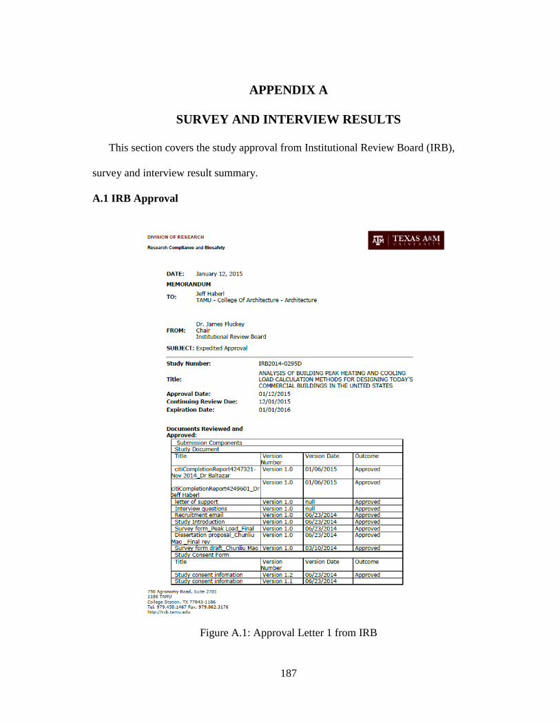
187
APPENDIX A
SURVEY AND INTERVIEW RESULTS
This section covers the study approval from Institutional Review Board (IRB),
survey and interview result summary.
A.1 IRB Approval
Figure A.1: Approval Letter 1 from IRB

188
Figure A.1 Continued

189
Figure A.2: Approval Letter 2 from IRB
190
Figure A.2 Continued

191
Figure A.3: Approval Letter 3 from IRB

192
Figure A.3 Continued
193
Figure A.3 Continued

194
A.2 Survey Results
Figure A.4: Survey Result for SFP 1

195
Figure A.5: Survey Result for SFP 2

196
Figure A.6: Survey Result for SFP 3

197
Figure A.7: Survey Result for SFP 4

198
Figure A.8: Survey Result for SFP 5

199
Figure A.9: Survey Result for SFP 6

200
Figure A.10: Survey Result for SFP 7

201
Figure A.11: Survey Result for SFP 8

202
Figure A.12: Survey Result for SFP 9
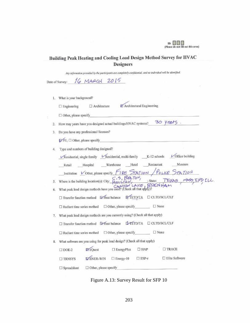
203
Figure A.13: Survey Result for SFP 10

204
Figure A.14: Survey Result for SFP 11

205
A.3 Interview Results
Figure A.15: Interview Result for SFP 2

206
Figure A.15 Continued

207
Figure A.15 Continued

208
Figure A.16: Interview Result for SFP 3

209
Figure A.16 Continued

210
Figure A.16 Continued

211
Figure A.17: Interview Result for SFP 4
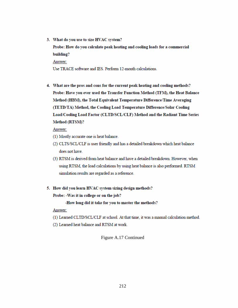
212
Figure A.17 Continued

213
Figure A.17 Continued

214
Figure A.18: Interview Result for SFP 6

215
Figure A.18 Continued

216
Figure A.18 Continued

217
Figure A.19: Interview Result for SFP 7

218
Figure A.19 Continued

219
Figure A.19 Continued

220
Figure A.20: Interview Result for SFP 8

221
Figure A.20 Continued

222
Figure A.20 Continued

223
Figure A.21: Interview Result for SFP 9

224
Figure A.21 Continued

225
Figure A.21 Continued

226
Figure A.22: Interview Result for SFP 10

227
Figure A.22 Continued

228
Figure A.22 Continued

229
Figure A.22 Continued

230
Figure A.23: Interview Result for SFP 11

231
Figure A.23 Continued

232
Figure A.23 Continued

233
APPENDIX B
CALCULATIONS OF SOLAR RADIATION AND SOL-AIR
TEMPERATURE
B.1 Solar Time and Solar Angles
Two solar angles are involved in order to calculate solar intensities, which are solar
altitude and solar incidence angle by (ASHRAE, 2013a). To start with, solar time can be
determined,
/ 60 ( ) /15AST LST ET LON LSM (B.1)
where,
AST : apparent solar time, hour;
LST : local standard time, hour;
ET : equation of time, min;
LON : longitude of site, degree;
LSM : longitude of local standard time meridian, degree.
The solar altitude β can be calculated by,
sin cos cos cos sin sinL H L (B.2)
where,
L : latitude, degrees;
: declination, degrees;
H : hour angle, degrees.
234
The solar incidence angle θ can be given by,
cos cos cos sin cos cos (B.3)
where,
: surface solar azimuth, degrees;
: surface tilt, degrees.
B.2 The ASHRAE Clear-Sky Models
The ASHRAE clear-sky radiation models are used to calculate beam, diffuse and
total solar radiation, which are the basis to calculate solar irradiation on the building
exterior surfaces. Two models have been proposed by the ASHRAE. The first ASHRAE
clear-sky model was first proposed in 1967 (ASHRAE, 1967) and utilizes three
coefficients (A, B, C) to perform the solar radiation calculations. This model was
replaced by a new ASHRAE clear-sky model in 2009 based on calculation components
such as beam optical depth, diffuse optical depth, beam air mass exponent, and diffuse
air mass exponent (ASHRAE, 2009d).
B.2.1 The 1967 ASHRAE Clear-Sky Model
The 1967 ASHRAE clear-sky model was adopted to calculate solar radiation before
2009. When calculating peak cooling loads, the assumption of a clear sky is selected in
order to account for the worst summer condition. This allows the most solar heat gain
into the building. The model involves A, B, C coefficients and atmosphere clearness to
perform the calculations. Two different sets of A, B, C coefficients have been published
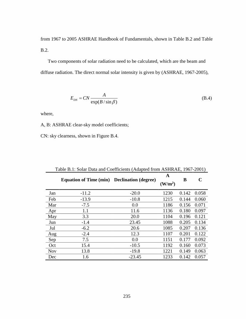
235
from 1967 to 2005 ASHRAE Handbook of Fundamentals, shown in Table B.2 and Table
B.2.
Two components of solar radiation need to be calculated, which are the beam and
diffuse radiation. The direct normal solar intensity is given by (ASHRAE, 1967-2005),
exp( / sin )DN
AE CN
B (B.4)
where,
A, B: ASHRAE clear-sky model coefficients;
CN: sky clearness, shown in Figure B.4.
Table B.1: Solar Data and Coefficients (Adapted from ASHRAE, 1967-2001)
Equation of Time (min) Declination (degree) A
(W/m2) B C
Jan -11.2 -20.0 1230 0.142 0.058
Feb -13.9 -10.8 1215 0.144 0.060
Mar -7.5 0.0 1186 0.156 0.071
Apr 1.1 11.6 1136 0.180 0.097
May 3.3 20.0 1104 0.196 0.121
Jun -1.4 23.45 1088 0.205 0.134
Jul -6.2 20.6 1085 0.207 0.136
Aug -2.4 12.3 1107 0.201 0.122
Sep 7.5 0.0 1151 0.177 0.092
Oct 15.4 -10.5 1192 0.160 0.073
Nov 13.8 -19.8 1221 0.149 0.063
Dec 1.6 -23.45 1233 0.142 0.057
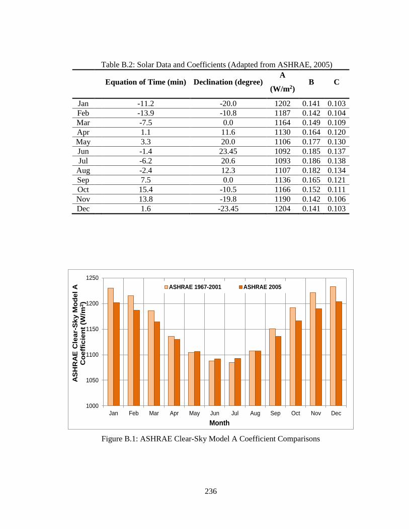
236
Table B.2: Solar Data and Coefficients (Adapted from ASHRAE, 2005)
Equation of Time (min) Declination (degree) A
(W/m2) B C
Jan -11.2 -20.0 1202 0.141 0.103
Feb -13.9 -10.8 1187 0.142 0.104
Mar -7.5 0.0 1164 0.149 0.109
Apr 1.1 11.6 1130 0.164 0.120
May 3.3 20.0 1106 0.177 0.130
Jun -1.4 23.45 1092 0.185 0.137
Jul -6.2 20.6 1093 0.186 0.138
Aug -2.4 12.3 1107 0.182 0.134
Sep 7.5 0.0 1136 0.165 0.121
Oct 15.4 -10.5 1166 0.152 0.111
Nov 13.8 -19.8 1190 0.142 0.106
Dec 1.6 -23.45 1204 0.141 0.103
1000
1050
1100
1150
1200
1250
Jan Feb Mar Apr May Jun Jul Aug Sep Oct Nov Dec
AS
HR
AE
Cle
ar-
Sk
y M
od
el A
C
oe
ffic
ien
t (W
/m2)
Month
ASHRAE 1967-2001 ASHRAE 2005
Figure B.1: ASHRAE Clear-Sky Model A Coefficient Comparisons

237
0.00
0.05
0.10
0.15
0.20
0.25
Jan Feb Mar Apr May Jun Jul Aug Sep Oct Nov Dec
AS
HR
AE
Cle
ar-
Sk
y M
od
el
B
Co
eff
icie
nt
(Dim
en
sio
nle
ss
)
Month
ASHRAE 1967-2001 ASHRAE 2005
Figure B.2: ASHRAE Clear-Sky Model B Coefficient Comparisons
0.00
0.02
0.04
0.06
0.08
0.10
0.12
0.14
0.16
Jan Feb Mar Apr May Jun Jul Aug Sep Oct Nov Dec
AS
HR
AE
Cle
ar-
Sk
y M
od
el
C
Co
eff
icie
nt
(Dim
en
sio
nle
ss
)
Month
ASHRAE 1967-2001 ASHRAE 2005
Figure B.3: ASHRAE Clear-Sky Model C Coefficient Comparisons
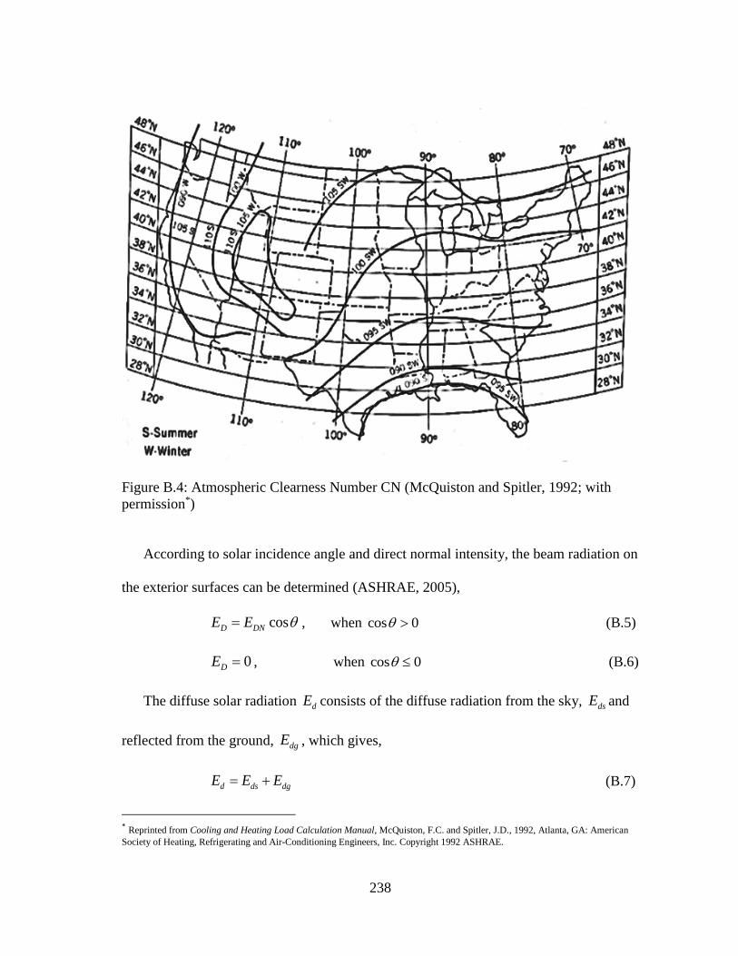
238
Figure B.4: Atmospheric Clearness Number CN (McQuiston and Spitler, 1992; with
permission*)
According to solar incidence angle and direct normal intensity, the beam radiation on
the exterior surfaces can be determined (ASHRAE, 2005),
cosD DNE E , when cos 0 (B.5)
0DE , when cos 0 (B.6)
The diffuse solar radiation dE consists of the diffuse radiation from the sky, dsE and
reflected from the ground, dgE , which gives,
d ds dgE E E (B.7)
* Reprinted from Cooling and Heating Load Calculation Manual, McQuiston, F.C. and Spitler, J.D., 1992, Atlanta, GA: American
Society of Heating, Refrigerating and Air-Conditioning Engineers, Inc. Copyright 1992 ASHRAE.
239
For vertical surfaces,
ds DNE CYE (B.8)
0.5 ( sin )dg DN gE E C (B.9)
For other surfaces,
(1 cos ) / 2ds DNE CE (B.10)
( sin ) (1 cos ) / 2dg DN gE E C (B.11)
where,
C: ASHRAE clear-sky model coefficients;
g : ground reflectance.
Prior to calculating diffuse component of solar radiation, a ratio Y has to be
determined first, which represents a fraction of diffuse solar radiation incidence on the
exterior vertical surface over the ones on the horizontal surface. The calculations yield,
20.55 0.437cos 0.313cosY , when cos 0.2 (B.12)
0.45Y , when cos 0.2 (B.13)
The total solar radiation intensities on the exterior surfaces are calculated by,
t D dE E E (B.14)
B.2.2 The 2009 ASHRAE Clear-Sky Model
The updated 2009 ASHRAE clear-sky model was developed by Thevenard in
ASHRAE Research Project RP 1453 (ASHRAE, 2009d) and introduced in the 2009
ASHRAE Handbook of Fundamentals (ASHRAE, 2009c). The calculations of solar

240
radiation under clear-sky condition involves parameters of extraterrestrial normal
irradiance 0E , air mass m , beam optical depth b , diffuse optical depth d , beam air
mass exponent ab , and diffuse air mass exponent ad . The 2013 ASHRAE Handbook of
Fundamentals (ASHRAE, 2013a) updated the equation coefficients of determining bean
and diffuse air mass exponents.
Extraterrestrial normal irradiance 0E can be obtained either from ASHRAE
tabulated table or calculated by the equation.
Table B.3: Extraterrestrial Normal Irradiance 0E for 21st Day of Each Month (Adapted
from ASHRAE, 2013a)
Month Jan Feb Mar Apr May Jun Jul Aug Sep Oct Nov Dec
Day of Year 21 52 80 111 141 172 202 233 264 294 325 355
0E , W/m2 1410 1397 1378 1354 1334 1323 1324 1336 1357 1380 1400 1400
0
3{1 0.033cos[360 ]}
365sc
nE E
(B.15)
where,
scE :solar constant;
n : the day of year.
Air mass m can be calculated by,
1.63641/ [sin 0.50572(6.07995 ) ]m (B.16)
where, is solar altitude, in degrees.
241
Air mass exponents are given by30,
1.454 0.406 0.268 0.021b d b dab (B.17)
0.507 0.205 0.080 0.190b d b dad (B.18)
where,
b : beam optical depth;
d : diffuse optical depth.
Therefore, the beam normal irradiance bE and diffuse horizontal irradiation dE are,
0 exp[ ]ab
b bE E m (B.19)
0 exp[ ]ad
d dE E m (B.20)
Given by incidence angle, the beam irradiance on the exterior surfaces ,t bE are
calculated by,
, cost b bE E , when cos 0 (B.21)
, 0t bE , when cos 0 (B.22)
To calculate diffuse irradiance on the exterior surface from the sky ,t dE , the ratio Y
is also used in the 2009 ASHRAE clear-sky model. This can be calculated by,
,t d dE E Y , for vertical surfaces (B.23)
For non-vertical surfaces with slope ,
, ( sin cos )t d dE E Y , when 90 (B.24)
30 The coefficients are different from the ones in the 2009 ASHRAE Handbook of Fundamentals.
242
, sint d dE E Y , when 90 (B.25)
Finally, the diffuse irradiance on the exterior surfaces from the ground reflectance
,t rE is determined by,
,
1 cos( sin )
2t r b d gE E E
(B.26)
The total solar radiation intensities on the exterior surfaces are given by,
, , ,t t b t d t rE E E E (B.27)
B.2.3 The ASHRAE Clear-Sky Model Comparisons
This section presents the comparisons of 1967 and 2009 ASHRAE clear-sky models.
Stillwater, OK and College Station, TX are the selected cities for comparisons. The date
of the weather conditions is September 22nd in 2001.
Figure B.5 shows the ASHRAE clear-sky model comparisons for Stillwater, OK.
This city is selected because it is where the experiments were performed by Oklahoma
State University for validating the HBM and RTSM. In the figure, direct normal, beam,
diffuse, and total horizontal solar irradiance predicted by three models are presented. For
the 1967 ASHRAE model, the two sets of A, B, C coefficients provide roughly equal
direct normal solar irradiance. This is because the A and B changes have a small impact.
The same observations were found for the beam solar irradiance, because it is calculated
by direct normal solar irradiance multiplied by the cosine of the incidence angle ( cos ).
However, the c coefficients for September increases 32%, compared to the first
published number, and the diffuse solar irradiance appears to be different, as shown in
243
Figure B.5. The second sets of coefficients tend to over-predict the diffuse solar
compared to the first set, which makes the total solar irradiance larger than the one
predicted using the first sets of A, B, C coefficients. The 2009 ASHRAE model
estimates a larger beam solar irradiance component compared to the 1967 ASHRAE
model. The diffuse solar irradiance from the 2009 ASHRAE model is between the
values predicted by the 1967 ASHRAE model using two sets of A, B, C coefficients.
The total solar irradiance by 2009 ASHRAE model is the largest among all methods.
Figure B.6 reveals the ASHRAE clear-sky model comparisons for College Station,
TX. The same observations from the 1967 ASHRAE models with the two sets of
coefficients are the same. However, the beam solar irradiance from the 2009 ASHRAE
model is underestimated, compared to the 1967 ASHRAE model. Similar to Stillwater,
OK, the diffuse solar irradiance from the 2009 ASHRAE model is between the values
predicted by the 1967 ASHRAE model using the two sets of A, B, C coefficients. The
total solar irradiance from the 2009 ASHRAE model gives roughly the same estimates as
the 1967 ASHRAE model using the first set of coefficients. However, it is smaller than
the numbers predicted by the 1967 ASHRAE model using the second sets of
coefficients.

244
0
100
200
300
400
500
600
700
800
900
1000
0 2 4 6 8 10 12 14 16 18 20 22 24
(W/m
2)
Time
Stillwater
Direct Normal(1967 ASHRAE 1)
Beam(1967 ASHRAE 1)
Diffuse(1967 ASHRAE 1)
Total Horizontal (1967 ASHRAE 1)
Direct Norma l(1967 ASHRAE 2)
Beam (1967 ASHRAE 2)
Diffuse (1967 ASHRAE 2)
Total Horizontal (1967 ASHRAE 2)
Beam (2009 ASHRAE)
Diffuse (2009 ASHRAE)
Total Horizontal (2009 ASHRAE)
Figure B.5: ASHRAE Clear-Sky Model Comparisons for Stillwater, OK City
0
100
200
300
400
500
600
700
800
900
1000
0 2 4 6 8 10 12 14 16 18 20 22 24
(W/m
2)
Time
College Station
Direct Normal(1967 ASHRAE 1)
Beam(1967 ASHRAE 1)
Diffuse(1967 ASHRAE 1)
Total Horizontal (1967 ASHRAE1)Direct Norma l(1967 ASHRAE 2)
Beam (1967 ASHRAE 2)
Diffuse (1967 ASHRAE 2)
Total Horizontal (1967 ASHRAE2)Beam (2009 ASHRAE)
Diffuse (2009 ASHRAE)
Total Horizontal (2009 ASHRAE)
Figure B.6: ASHRAE Clear-Sky Model Comparisons for College Station, TX City

245
B.3 Sol-Air Temperature
Sol-air temperature et is defined as “the temperature of the outdoor air that, in the
absence of all radiation changes, gives the same rate of heat entry into the surface as
would the combination of incident solar radiation, radiant energy exchange with the sky
and other outdoor surroundings, and convective heat exchanges with the outdoor air”
(ASHRAE, 2013a). This concept was originally introduced by Mackey and Wright in
1944. They also proposed an equation to calculate building inside surface temperature by
daily average sol-air temperature, a decrement factor and a lag angle. Later, sol-air
temperature was introduced into ASHRAE as the foundation of the ASHRAE simplified
peak cooling load methods to calculate building sensible cooling load.
Usually, the conduction heat gain q transferred into the building exterior surfaces
can be determined by (ASHRAE, 2013a),
/ ( )t o o sq A E h t t R (B.28)
where,
A : exterior surface area, m2;
: exterior surface solar absorptance;
tE : total solar radiation intensities on the exterior surface, W/m2;
oh : combined heat transfer coefficient that includes long-wave radiation and convection
at the exterior surface, W/m2-K;
ot : outdoor dry bulb temperature, C;
st : exterior surface temperature, C;

246
: hemispherical surface emittance;
R : difference between the long-wave radiation incident on the surface from the sky
and surroundings and the radiation emitted by a blackbody at outdoor air temperature,
W/m2; 63 W/m2 for horizontal surfaces and 0 W/m2 for vertical surfaces.
Assume the same heat gain can be provided using sol-air temperature concept,
/ ( )o e sq A h t t (B.29)
Inserting Equation (B.28) into Equation (B.29), the sol-air temperature et can be
obtained,
/ /e o t o ot t E h R h (B.30)
In practice, / oR h is assumed to be 4 K and 0 K for horizontal and vertical
surfaces, respectively.
247
APPENDIX C
FENESTRATION SOLAR HEAT GAIN MODELS
There are two fenestration models for calculating solar heat gains available in
ASHRAE. One model relies on the Transmitted Solar Heat Gain Factor (TSHGF),
Absorbed Solar Heat Gain Factor (ASHGF), and Shading Coefficient (SC) to perform
solar heat gains through the fenestration (McQuiston and Spitler, 1992). The other model
uses the incidence angle-based Solar Heat Gain Coefficient (SHGC) and Indoor
Attenuation Coefficient (IAC) to calculate solar heat gains (ASHRAE, 2013a; Nigusse,
2007).
C.1 Overview of Fenestration Solar Heat Gains
The incoming solar consists of beam and diffuse solar radiation. For a single pane,
clear window exposed to the solar radiation, of the 100% incoming solar radiation,
approximately 80% is transmitted thru the window glazing, while 8% is reflected to the
outside space. The remaining 12% is absorbed by the window glazing. Of this amount,
only 4% of it goes into the space, called the “inward flow”, and 8% goes to the outside,
called the “outward flow”. Therefore, to count for the solar heat gains through the
fenestration, both transmitted solar and the inward flow of the absorbed solar need to be
determined, see Figure C.1.
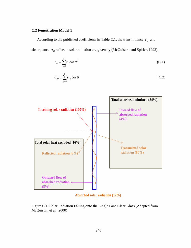
248
C.2 Fenestration Model 1
According to the published coefficients in Table C.1, the transmittance D and
absorptance D of beam solar radiation are given by (McQuiston and Spitler, 1992),
5
0
cos j
D j
j
t
(C.1)
5
0
cos j
D j
j
(C.2)
Incoming solar radiation (100%)
Reflected radiation (8%)
Transmitted solar
radiation (80%)
Absorbed solar radiation (12%)
Inward flow of
absorbed radiation
(4%)
Outward flow of
absorbed radiation
(8%)
Total solar heat admitted (84%)
Total solar heat excluded (16%)
Figure C.1: Solar Radiation Falling onto the Single Pane Clear Glass (Adapted from
McQuiston et al., 2000)
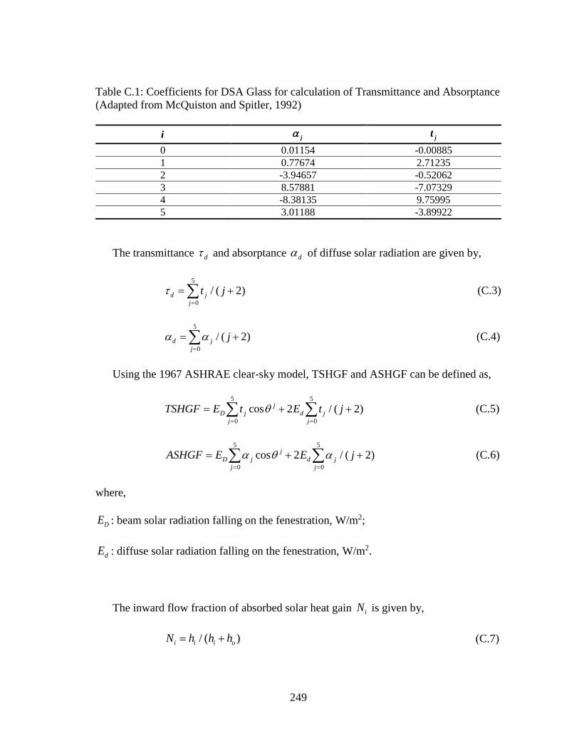
249
Table C.1: Coefficients for DSA Glass for calculation of Transmittance and Absorptance
(Adapted from McQuiston and Spitler, 1992)
i j jt
0 0.01154 -0.00885
1 0.77674 2.71235
2 -3.94657 -0.52062
3 8.57881 -7.07329
4 -8.38135 9.75995
5 3.01188 -3.89922
The transmittance d and absorptance d of diffuse solar radiation are given by,
5
0
/ ( 2)d j
j
t j
(C.3)
5
0
/ ( 2)d j
j
j
(C.4)
Using the 1967 ASHRAE clear-sky model, TSHGF and ASHGF can be defined as,
5 5
0 0
cos 2 / ( 2)j
D j d j
j j
TSHGF E t E t j
(C.5)
5 5
0 0
cos 2 / ( 2)j
D j d j
j j
ASHGF E E j
(C.6)
where,
DE : beam solar radiation falling on the fenestration, W/m2;
dE : diffuse solar radiation falling on the fenestration, W/m2.
The inward flow fraction of absorbed solar heat gain iN is given by,
/ ( )i i i oN h h h (C.7)

250
where,
ih : heat transfer coefficient at inner surface, W/m2-K;
oh : heat transfer coefficient at outer surface, W/m2-K.
Using Eqns (C.5), (C.6) and (C.7), the transmitted solar heat gain (TSHG) and
absorbed solar heat gain (ASHG) yield,
( )TSHG TSHGF SC A (C.8)
( ) iASHG ASHGF SC N A (C.9)
where,
SC : shading coefficient;
A : window surface area, m2.
C.3 Fenestration Model 2
Instead of separately calculating transmitted and absorbed solar radiation through the
fenestration, another way is to calculate beam and diffuse solar radiation by using
incidence angle-based SHGC and IAC. The transmitted and the inward flow of absorbed
solar is considered in the SHGC. Using the 2009 ASHRAE clear-sky model, the beam
and diffuse solar heat gains thru the fenestration are given by (ASHRAE, 2013a),
, ( ) ( , )b t bq AE SHGC IAC (C.10)
, ,( )d t d t r DDq A E E SHGC IAC (C.11)
where,

251
A : window surface area, m2;
,r bE : beam solar radiation falling on the fenestration, W/m2;
,t dE : diffuse solar radiation from the sky falling on the fenestration, W/m2;
,t rE : diffuse solar radiation from the ground reflection falling on the fenestration, W/m2;
( )SHGC : incidence angle based beam solar heat gain coefficient;
DSHGC : diffuse solar heat gain coefficient;
( , )IAC : indoor solar attenuation coefficient for beam solar heat gain coefficient;
DIAC : indoor solar attenuation coefficient for diffuse solar heat gain coefficient.
C.4 Fenestration Model Comparison
Figure C.2 shows the total fenestration solar heat gain comparison using two
fenestration models for the base case in the current study.
0
1,000
2,000
3,000
4,000
5,000
6,000
7,000
12:00 AM 3:00 AM 6:00 AM 9:00 AM 12:00 PM 3:00 PM 6:00 PM 9:00 PM 12:00 AM
(W)
Time
Fenestration Model 1(using SC)
Fenestration Model 2 (Using SHGC)
Figure C.2: Total Fenestration Solar Heat Gain Comparison Using Fenestration Model 1
and 2 for Base Case on September 22nd 2001, Stillwater, OK.
252
APPENDIX D
HEAT BALANCE METHOD (HBM)
This section presents the heat balance method, which is used to calculate building
peak loads. According to 2013 ASHRAE Handbook of Fundamentals, the following
assumptions and processes must be considered for the HBM:
The zone air temperature is well mixed and uniform;
The zone surfaces have uniform surface temperatures;
The zone has uniform long-wave and short-wave irradiation;
The zone has diffuse radiative surfaces;
The heat conduction process is one-dimensional.
The HBM includes four sub-calculations,
Outside surface heat balance;
Wall conduction process;
Inside surface heat balance;
Zone air heat balance.
D.1 Outside Surface Heat Balance
The heat balance at the outside surface is given by (ASHRAE, 2013a),
" " " " 0,sol LWR conv koq q q q (D.1)
where,
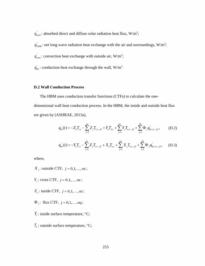
253
"
solq : absorbed direct and diffuse solar radiation heat flux, W/m2;
"
LWRq : net long wave radiation heat exchange with the air and surroundings, W/m2;
"
convq : convection heat exchange with outside air, W/m2;
"
koq : conduction heat exchange through the wall, W/m2.
D.2 Wall Conduction Process
The HBM uses conduction transfer functions (CTFs) to calculate the one-
dimensional wall heat conduction process. In the HBM, the inside and outside heat flux
are given by (ASHRAE, 2013a),
" "
, , , , , ,
1 1 1
( ) ,nqnz nz
ki o i t j i t j o o t j o t j j ki i t j
j j j
q t Z T Z T Y T Y T q
(D.2)
" "
, , , , , ,
1 1 1
( ) ,nqnz nz
ko o i t j i t j o o t j o t j j ko i t j
j j i
q t Y T Z T X T X T q
(D.3)
where,
jX : outside CTF, 0,1, ,j nz ;
jY : cross CTF, 0,1, ,j nz ;
jZ : inside CTF, 0,1, ,j nz ;
j : flux CTF, 0,1, ,j nq ;
iT : inside surface temperature, C;
oT : outside surface temperature, C;

254
"
kiq : conduction heat flux on inside face, W/m2;
"
koq : conduction heat flux on outside face, W/m2.
D.3 Inside Surface Heat Balance
The inside surface heat balance is modeled as a heat exchange among conduction
process, the convection to the room air, and the shortwave and long wave radiation
inside the zone. For each surface, it can be given by (ASHRAE, 2013a),
" " " " " " 0,LWX SW LWS ki sol convq q q q q q (D.4)
where,
"
LWXq : net long wave radiant exchange flux between zone surfaces, W/m2;
"
SWq : net shortwave radiation flux to surface from lights, W/m2;
"
LWSq : longwave radiation flux from equipment in zone, W/m2;
"
kiq : conduction flux through the wall, W/m2;
"
solq : transmitted solar radiation flux absorbed at the surface, W/m2;
"
convq : convection heat flux to the zone air, W/m2.
D.4 Air Heat Balance
By performing an air heat balance, the building cooling load can be obtained. The air
heat balance can be given by (ASHRAE, 2013a),
0,conv CE IV sysq q q q (D.5)

255
where,
convq : convection heat transfer from the surfaces, W;
CEq : convective part of internal loads, W;
IVq : sensible load due to infiltration and direct zone ventilation air, W;
sysq : heat transfer to/from the HVAC system, W.
D.5 Zone Heat Balance
A general zone heat balance procedure includes 12 surfaces, which are four walls,
four windows, one roof, one skylight, one floor, and thermal mass. This is shown in
Figure D.1.
Back Wall and Window
Floor
Roof and Skylight
Front wall and thermal mass are not shown
Figure D.1: Schematic View of General Heat Balance Zone (Adapted from ASHRAE,
2013a)
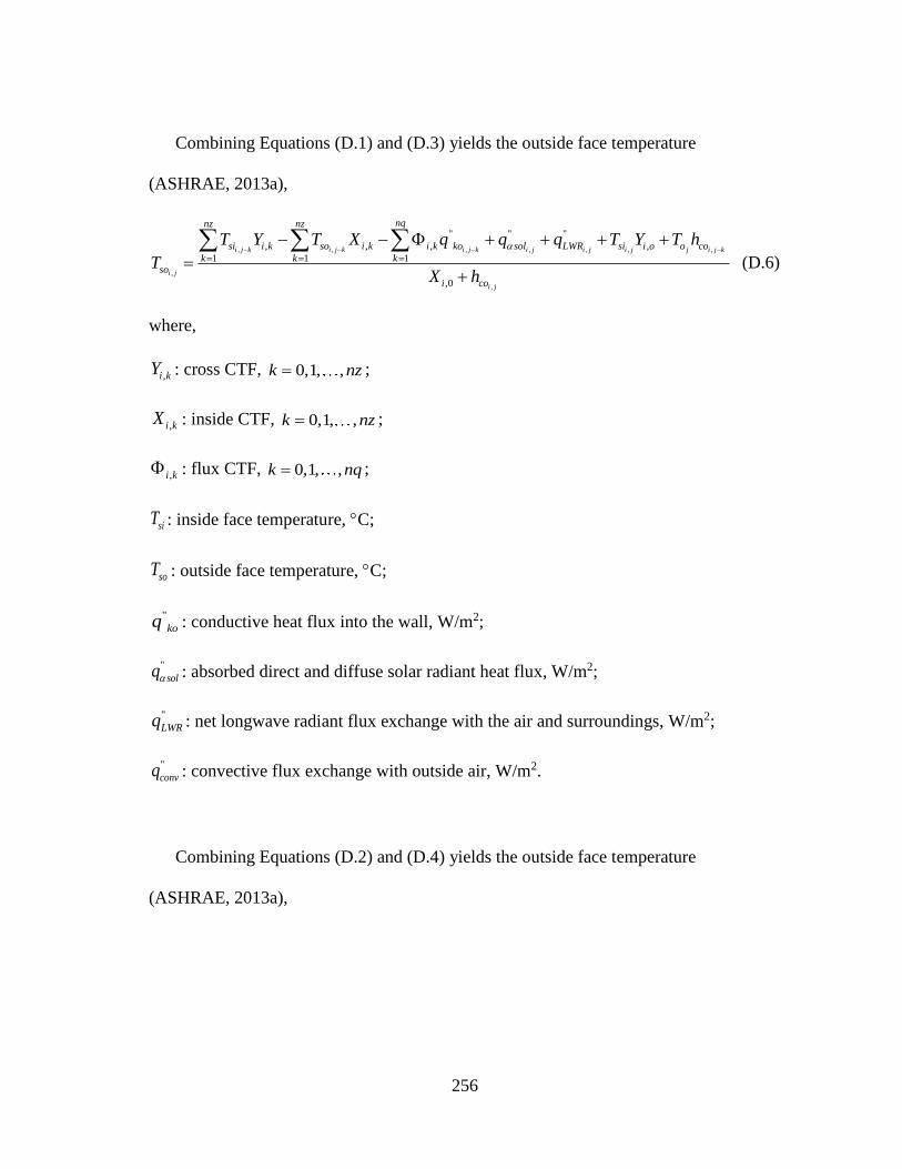
256
Combining Equations (D.1) and (D.3) yields the outside face temperature
(ASHRAE, 2013a),
, , , , , , ,
,
,
" " "
, , , ,
1 1 1
,0
i j k i j k i j k i j i j i j j i j k
i j
i j
nqnz nz
si i k so i k i k ko sol LWR si i o o co
k k kso
i co
T Y T X q q q T Y T h
TX h
(D.6)
where,
,i kY : cross CTF, 0,1, ,k nz ;
,i kX : inside CTF, 0,1, ,k nz ;
,i k : flux CTF, 0,1, ,k nq ;
siT : inside face temperature, C;
soT : outside face temperature, C;
"
koq : conductive heat flux into the wall, W/m2;
"
solq : absorbed direct and diffuse solar radiant heat flux, W/m2;
"
LWRq : net longwave radiant flux exchange with the air and surroundings, W/m2;
"
convq : convective flux exchange with outside air, W/m2.
Combining Equations (D.2) and (D.4) yields the outside face temperature
(ASHRAE, 2013a),
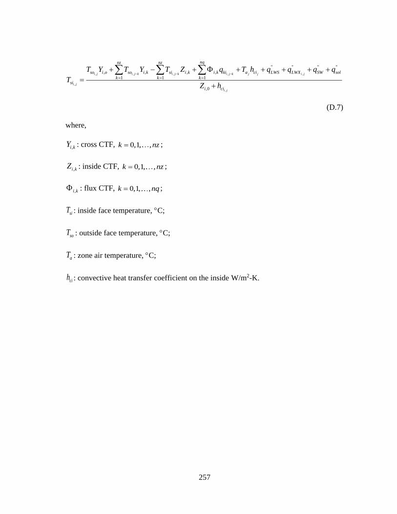
257
, , , , ,
,
,
" " " "
, , , ,
1 1 1
,0
i j i j k i j k i j k j j i j
i j
i j
nqnz nz
so i o so i k si i k i k ki a ci LWS LWX SW sol
k k ksi
i ci
T Y T Y T Z q T h q q q q
TZ h
(D.7)
where,
,i kY : cross CTF, 0,1, ,k nz ;
,i kZ : inside CTF, 0,1, ,k nz ;
,i k : flux CTF, 0,1, ,k nq ;
siT : inside face temperature, C;
soT : outside face temperature, C;
aT : zone air temperature, C;
cih : convective heat transfer coefficient on the inside W/m2-K.
258
APPENDIX E
RADIANT TIME SERIES METHOD (RTSM)
This section contains the details of radiant time series method procedure, which is
one of the simplified methods, compared to heat balance method. This method was first
introduced in 1997 by Spitler et al (Spitler, et al., 1997). Ten years later, it was improved
by Nigusse and Spitler (Nigusse, 2007; Nigusse and Spitler, 2010). The original RTSM
uses Periodic Response Factors (PRFs) to calculate the dynamic condition heat gains
through the opaque surfaces, while the improved RTSM introduces Conduction Time
Series Factors (CTSFs), a set of dimensionless factors, to perform the calculations. The
window solar heat gains are determined by solar heat gain coefficient (SHGC) in the
improved RTSM instead of shading coefficient (SC) used in original method. Here, the
original RTSM is called RTSM V1 and the later updated RTSM is called RTSM V2.
The overview flow charts of both methods are shown in Figure E.1 and Figure E.2,
respectively.
As one of the simplified methods for calculating building cooling loads, the RTSM is
implemented in both the ASHRAE LOADS Toolkit in the RTSM V1 and the ASHRAE
RTSM spreadsheet in the RTSM V2. Four types of heat gains are first determined,
including: conduction heat gains, solar heat gains through fenestration, internal heat
gains, and infiltration heat gain. All heat gains are split into radiative and convective
portions according to recommended split ratios. By applying radiant time series factors,
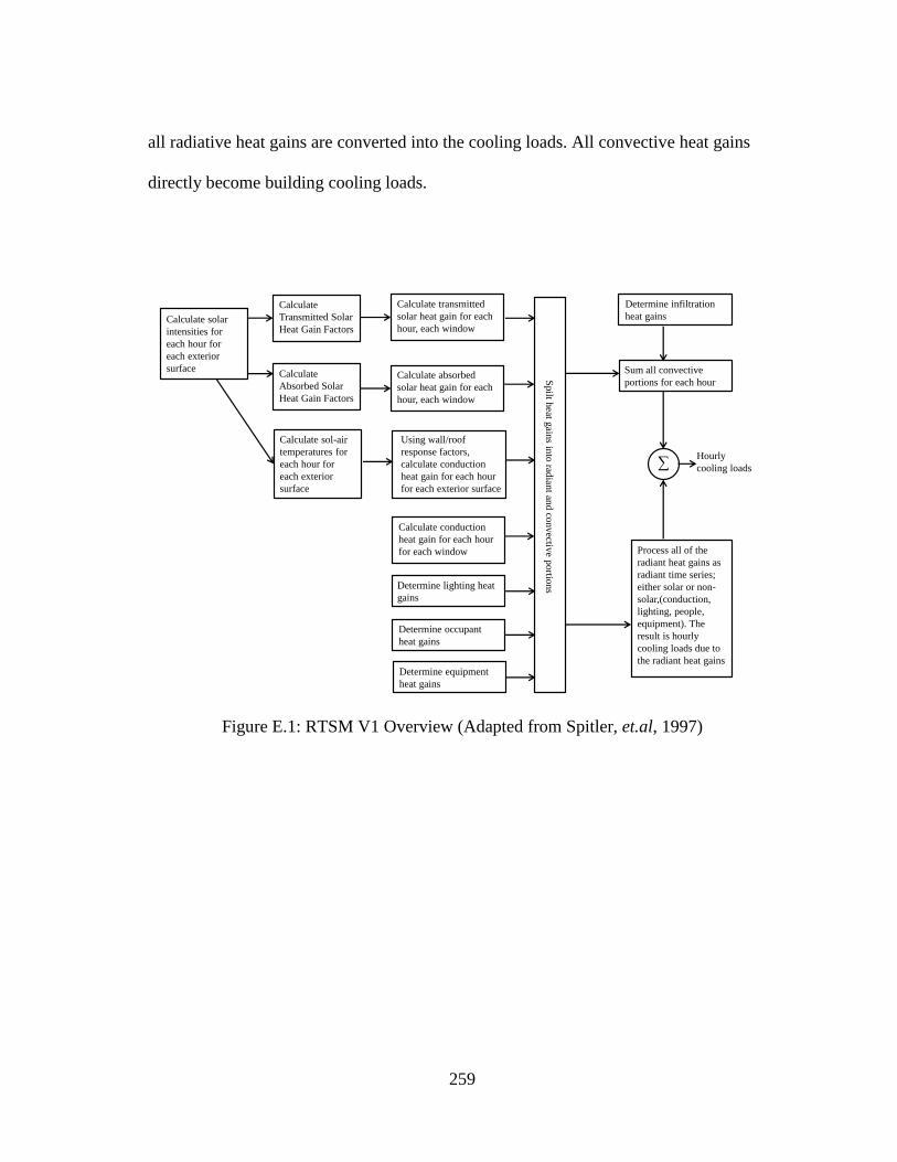
259
all radiative heat gains are converted into the cooling loads. All convective heat gains
directly become building cooling loads.
Calculate solar
intensities for
each hour for
each exterior
surface
Calculate
Transmitted Solar
Heat Gain Factors
Calculate
Absorbed Solar
Heat Gain Factors
Calculate sol-air
temperatures for
each hour for
each exterior
surface
Calculate transmitted
solar heat gain for each
hour, each window
Calculate absorbed
solar heat gain for each
hour, each window
Using wall/roof
response factors,
calculate conduction
heat gain for each hour
for each exterior surface
Calculate conduction
heat gain for each hour
for each window
Determine lighting heat
gains
Determine occupant
heat gains
Determine equipment
heat gains
Sp
ilt heat g
ains in
to rad
iant an
d co
nv
ective p
ortio
ns
Determine infiltration
heat gains
Sum all convective
portions for each hour
∑Hourly
cooling loads
Process all of the
radiant heat gains as
radiant time series;
either solar or non-
solar,(conduction,
lighting, people,
equipment). The
result is hourly
cooling loads due to
the radiant heat gains
Figure E.1: RTSM V1 Overview (Adapted from Spitler, et.al, 1997)
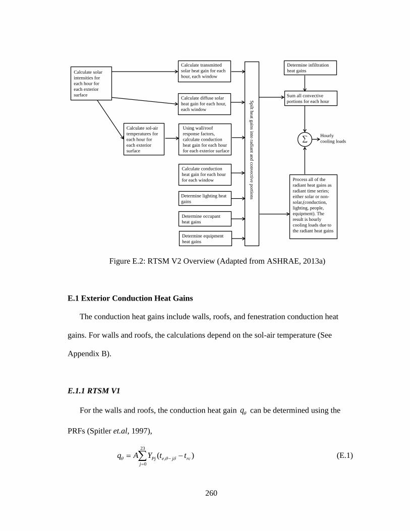
260
Calculate solar
intensities for
each hour for
each exterior
surface
Calculate sol-air
temperatures for
each hour for
each exterior
surface
Calculate transmitted
solar heat gain for each
hour, each window
Calculate diffuse solar
heat gain for each hour,
each window
Using wall/roof
response factors,
calculate conduction
heat gain for each hour
for each exterior surface
Calculate conduction
heat gain for each hour
for each window
Determine lighting heat
gains
Determine occupant
heat gains
Determine equipment
heat gains
Spilt h
eat gain
s into
radian
t and co
nvectiv
e portio
ns
Determine infiltration
heat gains
Sum all convective
portions for each hour
∑Hourly
cooling loads
Process all of the
radiant heat gains as
radiant time series;
either solar or non-
solar,(conduction,
lighting, people,
equipment). The
result is hourly
cooling loads due to
the radiant heat gains
Figure E.2: RTSM V2 Overview (Adapted from ASHRAE, 2013a)
E.1 Exterior Conduction Heat Gains
The conduction heat gains include walls, roofs, and fenestration conduction heat
gains. For walls and roofs, the calculations depend on the sol-air temperature (See
Appendix B).
E.1.1 RTSM V1
For the walls and roofs, the conduction heat gain q can be determined using the
PRFs (Spitler et.al, 1997),
23
,
0
( )Pj e j rc
j
q A Y t t
(E.1)

261
where,
A : exterior surface area, m2;
PjY : periodic response factor (PRFs), W/m2-K;
,e jt : sol-air temperature, j hour ago, C;
rct : constant room air temperature, C.
For fenestration conduction heat gains (ASHRAE, 2013a),
( )f out inq UA T T (E.2)
where,
U : overall U factor, W/m2-K;
A : window area, m2;
outT : outdoor temperature, C;
inT : indoor temperature, C.
E.1.2 RTSM V2
The RTSM V2 replaces the PRFs for the wall and roof conduction heat gain q can
be determined using dimensionless CTSFs (Spitler, 2009; ASHRAE, 2013a),
23
,
0
( )j e j rc
j
q c UA t t
(E.3)
where,
A : exterior surface area, m2;
262
jc : conduction time series factor (CTSF);
U : overall heat transfer coefficient for the surface, W/m2-K;
,e jt : sol-air temperature, j hour ago, C;
rct : constant room air temperature, C.
In the RTSM V2, the fenestration conduction heat gain is also calculated using Eqn
(E.2).
E.2 Fenestration Solar Heat Gains
The fenestration solar heat gain calculations are detailed in Appendix C. The RTSM
V1 adopts the fenestration model 1, while the RTSM V2 uses the fenestration model 2.
As previously mentioned, the fenestration model 1 uses the shading coefficient concept,
while the model 2 uses the SHGC and IAC involved in the calculation procedures.
E.3 Partition, Ceiling, Floor Conduction Heat Gains
According to the 2013 ASHRAE Handbook of Fundamentals Chapter 18, the
conduction heat gains for interior partitions, ceiling and floor can be calculated as a
steady state conduction heat transfer,
( )b iq UA t t (E.4)
where,
U : overall heat transfer coefficient between adjacent and conditioned space, W/m2-K;

263
A : surface area, m2;
bt : average air temperature in adjacent space, C;
it : air temperature in conditioned space, C.
E.4 Internal Heat Gains
Internal heat gains include occupancy, lighting, and equipment heat gains. According
to the 2013 ASHRAE Handbook of Fundamentals Chapter 18, they can be calculated as
follows:
For occupants,
,s s perq q N (E.5)
,l l perq q N (E.6)
where,
sq : total occupant sensible heat gain, W;
lq : total occupant latent heat gain, W;
,s perq : sensible heat gain per person W/person;
,l perq : latent heat gain per person, W/person;
N : number of occupants.
For lights,
el ul saq W F F (E.7)
264
where,
elq : lighting heat gain, W;
W : total light wattage, W;
ulF : lighting use factor, fraction;
saF : lighting special allowance factor, fraction;
For electric motors,
( / )em M UM LMq P E F F (E.8)
where,
emq : heat equivalent of equipment operation, W;
P : motor power rating, W;
ME : motor efficiency, fraction;
UMF : motor use factor, fraction;
LMF : motor load factor, fraction;
For hooded cooking appliances,
s input U Rq q F F (E.9)
where,
sq : sensible heat gain, W;
inputq : nameplate or rated energy input, W;
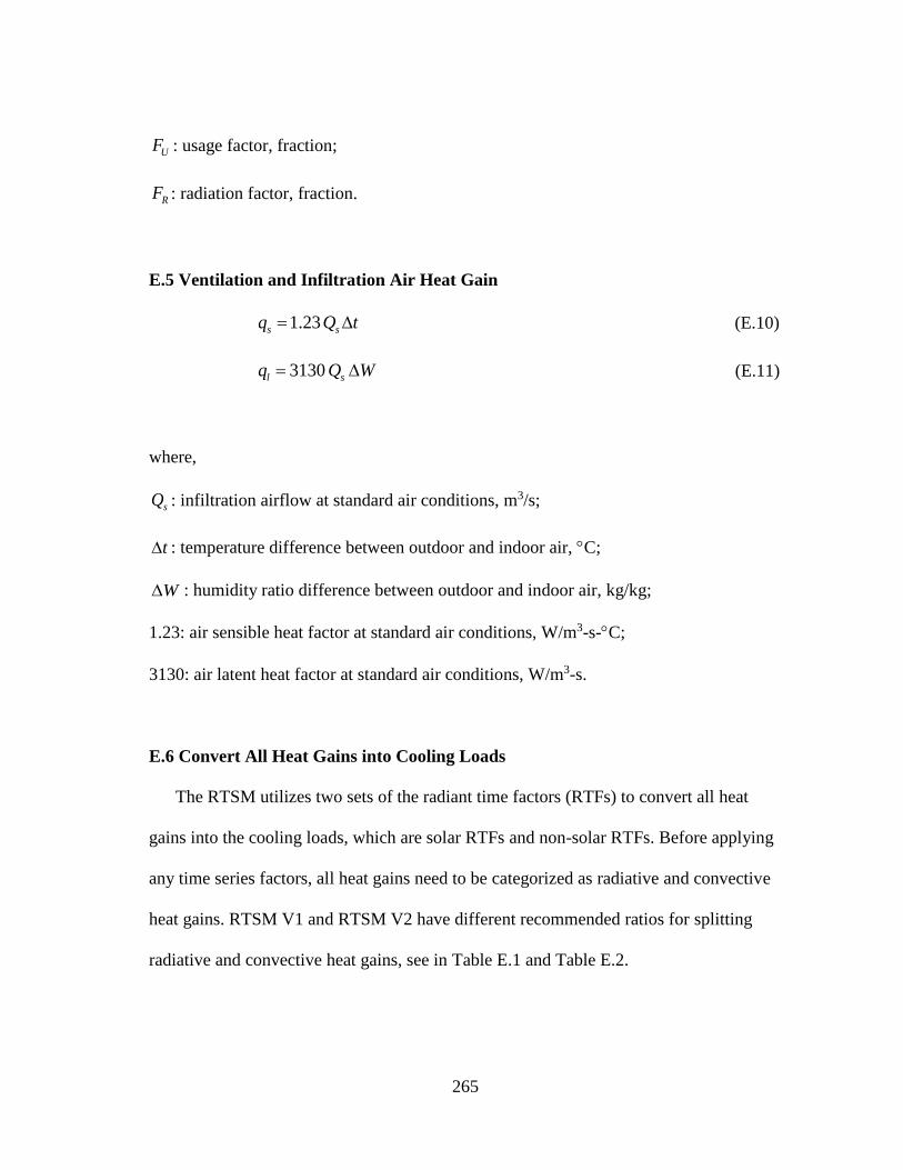
265
UF : usage factor, fraction;
RF : radiation factor, fraction.
E.5 Ventilation and Infiltration Air Heat Gain
1.23s sq Q t (E.10)
3130l sq Q W (E.11)
where,
sQ : infiltration airflow at standard air conditions, m3/s;
t : temperature difference between outdoor and indoor air, C;
W : humidity ratio difference between outdoor and indoor air, kg/kg;
1.23: air sensible heat factor at standard air conditions, W/m3-s-C;
3130: air latent heat factor at standard air conditions, W/m3-s.
E.6 Convert All Heat Gains into Cooling Loads
The RTSM utilizes two sets of the radiant time factors (RTFs) to convert all heat
gains into the cooling loads, which are solar RTFs and non-solar RTFs. Before applying
any time series factors, all heat gains need to be categorized as radiative and convective
heat gains. RTSM V1 and RTSM V2 have different recommended ratios for splitting
radiative and convective heat gains, see in Table E.1 and Table E.2.

266
The convective portion of heat gains directly become the cooling loads. However,
the radiative portion of heat gains must be absorbed by the interior surfaces or the
furniture, and then be convected into the space air temperature with a time delay. Two
sets of RTFs are applied to convert the radiative heat gains into the cooling load. The
solar beam heat gain is assumed to be distributed on the floor only, while other types of
heat gains are distributed uniformly to the interior surfaces, including radiative portion
of conduction heat gains and internal heat gains as well as diffuse solar heat gains.
Table E.1: Recommended Radiative-Convective Splits for Heat Gains for RTSM V1
(Adapted from Spitler et al., 1997)
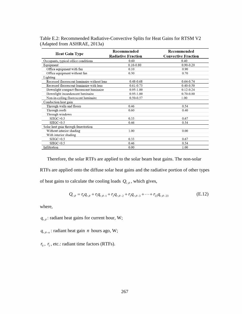
267
Table E.2: Recommended Radiative-Convective Splits for Heat Gains for RTSM V2
(Adapted from ASHRAE, 2013a)
Therefore, the solar RTFs are applied to the solar beam heat gains. The non-solar
RTFs are applied onto the diffuse solar heat gains and the radiative portion of other types
of heat gains to calculate the cooling loads ,rQ , which gives,
, 0 , 1 , 1 2 , 2 3 , 3 23 , 23r r r r r rQ r q r q r q r q r q (E.12)
where,
,rq : radiant heat gains for current hour, W;
,r nq : radiant heat gain n hours ago, W;
0r , 1r , etc.: radiant time factors (RTFs).

268
APPENDIX F
TRANSFER FUNCTION METHOD (TFM)
This section reviews the Transfer Function Method (TFM) for building peak load
calculations. It was first developed as a computer algorithm in 1972 (ASHRAE, 1972).
The TFM is a two-step, simplified method that incorporates the concepts of Conduction
Transfer Functions (CTFs) and Room Transfer Functions (RTFs, also called Weighting
Factors). Figure F.1 presents an overview of the methodology.
The TFM requires the solar intensities estimations for each exterior surface to
determine the sol-air temperatures. The conduction heat gains of walls and roofs are
calculated through sol-air temperatures and CTFS. The transmitted and absorbed solar
heat gains are calculated using the TSGHF and ASHGF, respectively. The fenestration
conduction heat gains can be obtained through steady state conduction heat transfer
process. If any internal heat gains exist, they need to be calculated individually. The
cooling loads from solar heat gains, conduction heat gains, and internal heat gains are
obtained applying the solar weighting factors, conduction weighting factors, lighting
weighting factors, and occupant/equipment weighting factors, respectively. The
infiltration heat gains directly contribute to the cooling load. Summing up all types of
cooling load can achieve the total cooling load for the space.

269
Calculate solar
intensities for
each hour for
each exterior
surface
Calculate
Transmitted Solar
Heat Gain
Factors(TSGHF)
Calculate
Absorbed Solar
Heat Gain Factors
(ASHGF)
Calculate sol-air
temperatures for
each hour for
each exterior
surface
Calculate transmitted
solar heat gain for each
hour, each window
Calculate absorbed
solar heat gain for each
hour, each window
Using conduction
transfer functions,
calculate conduction
heat gain for each hour
for each exterior surface
and any thermally
massive interior
surfaces separating
different temperature
needs
Calculate conduction
heat gain for each hour
for each window
Determine lighting heat
gains
Determine occupant
heat gains
Determine equipment
heat gains
∑
Using “Solar” WF
coefficients and
transmitted solar heat
gains, calculate hourly
cooling loads due to
transmitted solar heat
gain.
Using “Conduction”
WF coefficients and
sum of conduction heat
gains, absorbed solar
heat gains, calculate
hourly cooling loads
due to conduction heat
gain, absorbed solar
heat gains, and window
conduction heat gains.
Using “Lighting” WF
coefficients and lighting heat
gains, calculate hourly cooling
loads due to lighting
Using “Occupant/Equipment”
WF coefficients and sum of
occupant and equipment heat
gains, calculate hourly cooling
loads due to occupants and
equipment
Calculate infiltration loads
∑
Characterize
effects of
control system
If desired,
correct cooling
loads for effects
of control
system and
temperature
with space air
transfer
functions
∑
Figure F.1: TFM Overview (Adapted from McQuiston and Spitler, 1992)
F.1 Exterior Conduction Heat Gains
Relying on the CTFs, the conduction heat gains through walls and roofs can be
determined. Tabulated CTFs values are published by ASHRAE (ASHRAE, 1997). The
specific wall and roof layer combinations were first recommended by Harries and
McQuiston in 1988 (Harries and McQuiston, 1988). Forty-one types of walls and forty-
two types of roofs are available. Therefore, to use the TFM, it is needed to pick the
closest wall and roof combination types in the database.
In the TFM, the conduction heat gain through the walls and roofs is formulated by
(ASHRAE, 1997),

270
, , ,
0 1 0
[ ( / ) ]
e n e n n e n rc n
n n n
q A b t d q A t c (F.1)
where,
, e nq : heat gain through walls or roofs, Btu/h, at time n ;
A : wall or roof surface area, m2;
: current hour, h;
: time interval, h;
n : summation index, dimensionless;
, e nt : sol-air temperature at time n , C;
rct : indoor room temperature, C;
nb , nc : Conduction Transfer Function Coefficients, W/m2-K;
nd : Conduction Transfer Function Coefficients, dimensionless.
The TFM general procedure to determine the Conduction Transfer Function (CTF)
coefficients is detailed next.
Step 1: wall and roof material layers
The code names of wall and roof layers need to be selected from outside to inside
according to Table F.1, which shows the predetermined layer properties used in TFM.
Unfortunately, not all materials fall into the categories that are defined by Table F.1. In
such cases, the closest material needs to be selected. The full table of available materials
can be found in 1997 ASHRAE Handbook of Fundamentals.
271
Step 2: wall and roof group numbers
The determination of the wall group number is based on four parameters: principal
wall material; secondary wall material; R-value range; and mass location. The pre-
defined principal and secondary wall materials can be found in Table F.2 and Table F.3,
respectively. These two tables present the principal and secondary finishes with the
respective layer code numbers in the TFM. For instance, if the wall materials contain 4
in. heavy concrete and gypsum, the principal and the secondary wall material number
would be No. 8 and No. 1 accordingly. The wall R value range number can be chosen
from Table F.5 according to the overall wall R value. “Mass location” means the
principal wall material location relative to the insulation layer. Finally, mass location
needs to be determined from Table F.7.Three options are available: mass in; mass
integral; mass out. “Mass in” case represents the principal wall material is inside the wall
insulation. “Mass integral” case means the principal wall materials evenly distributed
among the wall insulation. “Mass out” case reveals the principal wall material lays
outside the wall insulation.
The wall group number can be determined by Table F.8. The column and row
numbers represents the principal material and R-value range numbers, respectively. In
the section of secondary material, the wall group number can be obtained. For example,
for a wall with principal material number 17 combined with secondary wall material A1
or/and E1, R-value range number 1 and a mass-in situation, the wall group number
would be No. 2.

272
Table F.1: Wall and Roof Layers Code Names and Thermal Properties31 (Adapted from
ASHRAE, 1997)
Code
Name Description
L
(mm)
k
(W/m-K)
ρ
(kg/m3)
cp
(kJ/kg-
K)
R
(m2-
K/W)
Mass
(kg/m2)
A0 Outside surface resistance 0 0.000 0 0.00 0.059 0.00
A1 25 mm Stucco 25 0.692 1858 0.84 0.037 47.34
A2 100 mm Face brick 100 1.333 2002 0.92 0.076 203.50
A3 Steel siding 2 44.998 7689 0.42 0.000 11.71
A4 12 mm Slag 13 0.190 1121 1.67 0.067 10.74
A5 Outside surface resistance 0 0.000 0 0.00 0.059 0.00
A6 Finish 13 0.415 1249 1.09 0.031 16.10
A7 100 mm Face brick 100 1.333 2002 0.92 0.076 203.50
B1 Air space resistance 0 0.000 0 0.00 0.160 0.00
B2 25 mm Insulation 25 0.043 32 0.84 0.587 0.98
B3 50 mm Insulation 51 0.043 32 0.84 1.173 1.46
C19 300 mm Low density
concrete block (filled) 300 0.138 304 0.84 2.200 92.72
C20 300 mm High density
concrete block (filled) 300 0.675 897 0.84 0.451 273.28
E0 Inside surface resistance 0 0.000 0 0.00 0.121 0.00
E1 20 mm Plaster or gypsum 20 0.727 1602 0.84 0.026 30.74
E2 12 mm Slag or stone 12 1.436 881 1.67 0.009 11.22
E3 10 mm Felt and membrane 10 0.190 1121 1.67 0.050 10.74
E4 Ceiling air space 0 0.000 0 0.00 0.176 0.00
E5 Acoustic title 19 0.061 481 0.84 0.314 9.27
Similarly, three parameters need to be known to determine a roof group number: roof
principal material; mass location parameter; R-value range number. Twenty principal
roof materials are available to be chosen in Table F.4. Three mass locations are listed in
Table F.7. The R-value range number can be picked in Table F.6.
The roof group number can be determined from Table F.9. The column is selected
based on the R value range number and the row number is chosen according to the roof
principal material.
31 This table shows partial material properties. Please check the full tables from 1997 ASHRAR Handbook of Fundamentals on page 28.19.
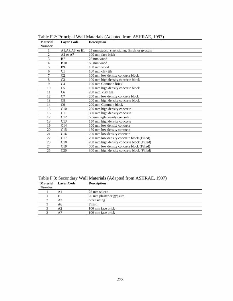
273
Table F.2: Principal Wall Materials (Adapted from ASHRAE, 1997) Material
Number
Layer Code Description
1 A1,A3,A6, or E1 25 mm stucco, steel siding, finish, or gypsum
2 A2 or A7 100 mm face brick
3 B7 25 mm wood
4 B10 50 mm wood
5 B9 100 mm wood
6 C1 100 mm clay tile
7 C2 100 mm low density concrete block
8 C3 100 mm high density concrete block
9 C4 100 mm Common brick
10 C5 100 mm high density concrete block
11 C6 200 mm. clay tile
12 C7 200 mm low density concrete block
13 C8 200 mm high density concrete block
14 C9 200 mm Common block
15 C10 200 mm high density concrete
16 C11 300 mm high density concrete
17 C12 50 mm high density concrete
18 C13 150 mm high density concrete
19 C14 100 mm low density concrete
20 C15 150 mm low density concrete
21 C16 200 mm low density concrete
22 C17 200 mm low density concrete block (Filled)
23 C18 200 mm high density concrete block (Filled)
24 C19 300 mm low density concrete block (Filled)
25 C20 300 mm high density concrete block (Filled)
Table F.3: Secondary Wall Materials (Adapted from ASHRAE, 1997) Material
Number
Layer Code Description
1 A1 25 mm stucco
1 E1 20 mm plaster or gypsum
2 A3 Steel siding
3 A6 Finish
3 A2 100 mm face brick
3 A7 100 mm face brick

274
Table F.4: Principal Roof Materials (Adapted from ASHRAE, 1997) Material
Number
Layer
Code
Description
1 B7 25 mm Wood
2 B8 65 mm. Wood
3 B9 100 mm Wood
4 C5 100 mm high density concrete block
5 C12 50 mm high density concrete
6 C13 150 mm high density concrete
7 C14 100 mm low density concrete
8 C15 150 mm low density concrete
9 C16 200 mm low density concrete
10 A3 Steel deck
11 B7 and E3 Attic ceiling combination
12 C12-C12 50 mm high density concrete (outer layer) to 50 mm high density concrete (inner layer)-
Roof Terrance System
13 C12-C5 50 mm high density concrete (outer layer) to 100 mm high density concrete block (inner
layer)-Roof Terrance System
14 C12-C13 50 mm high density concrete (outer layer) to 150 mm high density concrete (inner layer)-
Roof Terrance System
15 C5-C12 100 mm high density concrete block (outer layer) to 50 mm high density concrete (inner
layer)-Roof Terrance System
16 C5-C5 100 mm high density concrete block (outer layer) to 100 mm high density concrete block
(inner layer)-Roof Terrance System
17 C5-C13 100 mm high density concrete block (outer layer) to 150 mm high density concrete (inner
layer)-Roof Terrance System
18 C13-C12 150 mm high density concrete (outer layer) to 50 mm high density concrete (inner layer)-
Roof Terrance System
19 C13-C5 150 mm high density concrete (outer layer) to 100 mm high density concrete block (inner
layer)-Roof Terrance System
20 C13-C13 150 mm high density concrete (outer layer) to 150 mm high density concrete (inner layer)-
Roof Terrance System
Table F.5: Wall R-Value Range Definitions (Adapted from ASHRAE, 1997) R-Value Range Number R Value (m2-K/W)
1 0.00 - 0.35
2 0.35 – 0.44
3 0.44 – 0.53
4 0.53 – 0.62
5 0.62 – 0.70
6 0.70 – 0.84
7 0.84 – 0.97
8 0.97 – 1.14
9 1.14 – 1.36
10 1.36 – 1.58
11 1.58 – 1.89
12 1.89 – 2.24
13 2.24 – 2.64
14 2.64 – 3.08
15 3.08 – 3.52
16 3.52 – 4.05
17 4.05 – 4.76
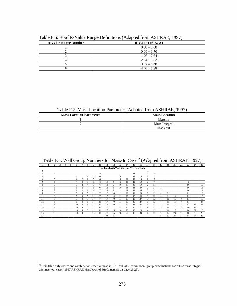
275
Table F.6: Roof R-Value Range Definitions (Adapted from ASHRAE, 1997) R-Value Range Number R Value (m2-K/W)
1 0.00 – 0.88
2 0.88 – 1.76
3 1.76 – 2.64
4 2.64 – 3.52
5 3.52 – 4.40
6 4.40 – 5.28
Table F.7: Mass Location Parameter (Adapted from ASHRAE, 1997) Mass Location Parameter Mass Location
1 Mass in
2 Mass Integral
3 Mass out
Table F.8: Wall Group Numbers for Mass-In Case32 (Adapted from ASHRAE, 1997) R 1 2 3 4 5 6 7 8 9 10 11 12 13 14 15 16 17 18 19 20 21 22 23 24 25
Combined with Wall Material A1, E1, or both
1 2
2 5 5 11 2 6
3 5 3 2 5 6 5 12 18 2 6
4 5 4 2 2 5 6 6 12 12 19 2 7
5 5 4 2 3 6 6 10 4 6 17 12 19 2 7 5
6 6 5 2 4 6 6 11 5 10 17 13 19 2 11 10 16
7 6 5 2 4 6 6 11 5 10 18 13 20 2 11 2 10 16
8 6 5 2 5 10 7 12 5 11 18 13 26 2 12 2 10 17
9 6 5 4 5 11 7 16 10 11 18 13 20 3 12 4 5 11 18
10 6 5 4 5 11 7 17 10 11 18 13 20 3 12 4 9 10 11 18
11 6 5 4 5 11 7 17 10 11 19 13 27 3 12 4 10 15 4 11 18
12 6 5 4 5 11 11 17 10 11 19 19 27 3 12 4 10 16 4 11 24
13 10 10 4 5 11 11 17 10 11 19 18 27 4 12 5 11 17 9 12 15 25
14 10 10 5 5 11 11 18 11 12 25 19 27 4 12 5 11 17 10 16 16 25
15 11 10 5 9 11 11 18 15 16 26 19 28 4 12 5 11 17 10 16 22 25
16 11 10 9 9 16 11 18 15 16 26 19 34 4 17 9 16 23 10 16 23 25
17 24 16 9 16 24 15 17 24 25
32 This table only shows one combination case for mass-in. The full table covers more group combinations as well as mass integral and mass out cases (1997 ASHRAE Handbook of Fundamentals on page 28.23).
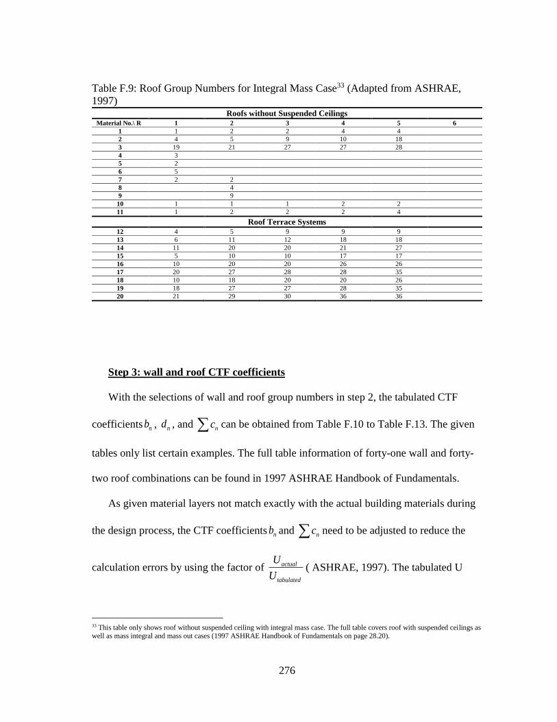
276
Table F.9: Roof Group Numbers for Integral Mass Case33 (Adapted from ASHRAE,
1997)
Roofs without Suspended Ceilings Material No.\ R 1 2 3 4 5 6
1 1 2 2 4 4
2 4 5 9 10 18
3 19 21 27 27 28
4 3
5 2
6 5
7 2 2
8 4
9 9
10 1 1 1 2 2
11 1 2 2 2 4
Roof Terrace Systems 12 4 5 9 9 9
13 6 11 12 18 18
14 11 20 20 21 27
15 5 10 10 17 17
16 10 20 20 26 26
17 20 27 28 28 35
18 10 18 20 20 26
19 18 27 27 28 35
20 21 29 30 36 36
Step 3: wall and roof CTF coefficients
With the selections of wall and roof group numbers in step 2, the tabulated CTF
coefficients nb , nd , and nc can be obtained from Table F.10 to Table F.13. The given
tables only list certain examples. The full table information of forty-one wall and forty-
two roof combinations can be found in 1997 ASHRAE Handbook of Fundamentals.
As given material layers not match exactly with the actual building materials during
the design process, the CTF coefficients nb and nc need to be adjusted to reduce the
calculation errors by using the factor of actual
tabulated
U
U( ASHRAE, 1997). The tabulated U
33 This table only shows roof without suspended ceiling with integral mass case. The full table covers roof with suspended ceilings as well as mass integral and mass out cases (1997 ASHRAE Handbook of Fundamentals on page 28.20).
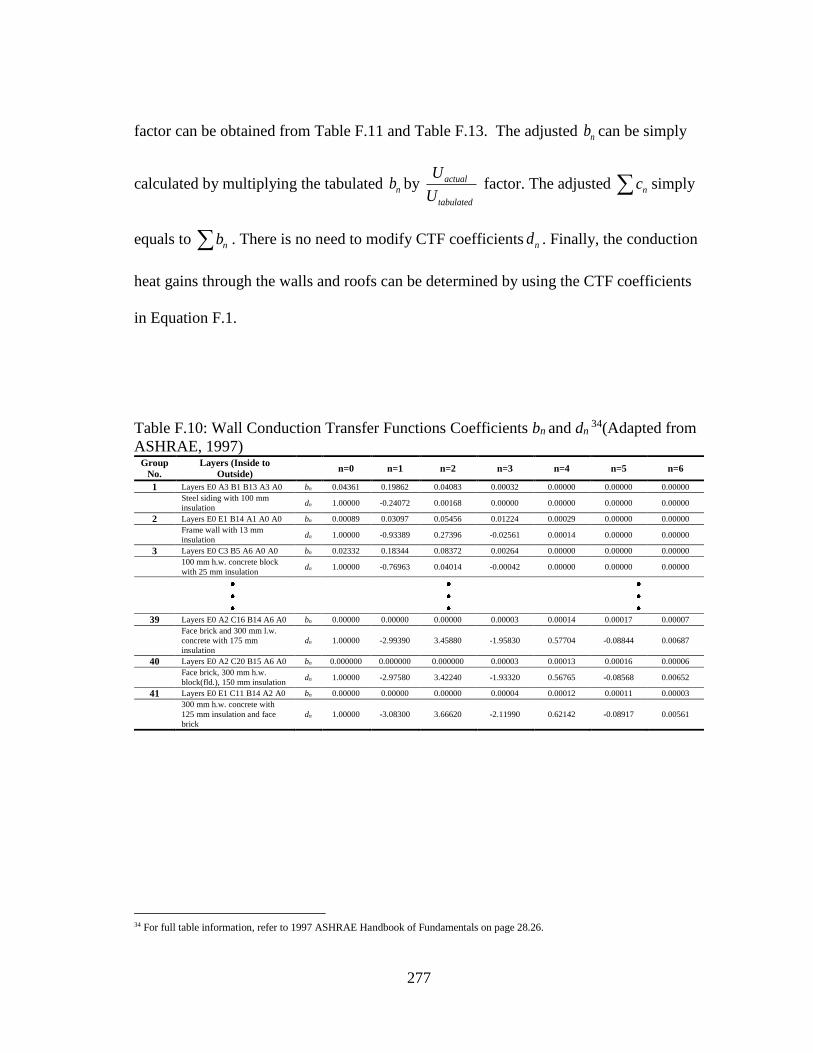
277
factor can be obtained from Table F.11 and Table F.13. The adjusted nb can be simply
calculated by multiplying the tabulated nb by actual
tabulated
U
U factor. The adjusted nc simply
equals to nb . There is no need to modify CTF coefficients nd . Finally, the conduction
heat gains through the walls and roofs can be determined by using the CTF coefficients
in Equation F.1.
Table F.10: Wall Conduction Transfer Functions Coefficients bn and dn
34(Adapted from
ASHRAE, 1997) Group
No.
Layers (Inside to
Outside) n=0 n=1 n=2 n=3 n=4 n=5 n=6
1 Layers E0 A3 B1 B13 A3 A0 bn 0.04361 0.19862 0.04083 0.00032 0.00000 0.00000 0.00000
Steel siding with 100 mm
insulation dn 1.00000 -0.24072 0.00168 0.00000 0.00000 0.00000 0.00000
2 Layers E0 E1 B14 A1 A0 A0 bn 0.00089 0.03097 0.05456 0.01224 0.00029 0.00000 0.00000
Frame wall with 13 mm
insulation dn 1.00000 -0.93389 0.27396 -0.02561 0.00014 0.00000 0.00000
3 Layers E0 C3 B5 A6 A0 A0 bn 0.02332 0.18344 0.08372 0.00264 0.00000 0.00000 0.00000
100 mm h.w. concrete block
with 25 mm insulation dn 1.00000 -0.76963 0.04014 -0.00042 0.00000 0.00000 0.00000
39 Layers E0 A2 C16 B14 A6 A0 bn 0.00000 0.00000 0.00000 0.00003 0.00014 0.00017 0.00007
Face brick and 300 mm l.w.
concrete with 175 mm
insulation
dn 1.00000 -2.99390 3.45880 -1.95830 0.57704 -0.08844 0.00687
40 Layers E0 A2 C20 B15 A6 A0 bn 0.000000 0.000000 0.000000 0.00003 0.00013 0.00016 0.00006
Face brick, 300 mm h.w.
block(fld.), 150 mm insulation dn 1.00000 -2.97580 3.42240 -1.93320 0.56765 -0.08568 0.00652
41 Layers E0 E1 C11 B14 A2 A0 bn 0.00000 0.00000 0.00000 0.00004 0.00012 0.00011 0.00003
300 mm h.w. concrete with
125 mm insulation and face
brick
dn 1.00000 -3.08300 3.66620 -2.11990 0.62142 -0.08917 0.00561
34 For full table information, refer to 1997 ASHRAE Handbook of Fundamentals on page 28.26.

278
Table F.11: Wall Conduction Transfer Functions Coefficients nc , Time Lag, U
Factor, and Decrement Factors 35(Adapted from ASHRAE, 1997)
Group
No. Layers (Inside to Outside) nc TL, h U DF
1 Layers E0 A3 B1 B13 A3 A0 0.283372 1.30 0.372389 0.98
2 Layers E0 E1 B14 A1 A0 A0 0.098947 3.21 0.314501 0.91
3 Layers E0 C3 B5 A6 A0 A0 0.29312 3.33 1.085249 0.78
39 Layers E0 A2 C16 B14 A6 A0 0.000416 14.64 0.227365 0.10
40 Layers E0 A2 C20 B15 A6 A0 0.00039 14.38 0.234753 0.08
41 Layers E0 E1 C11 B14 A2 A0 0.000296 14.87 0.294532 0.06
Table F.12: Roof Conduction Transfer Functions Coefficients bn and dn
36(Adapted from
ASHRAE, 1997) Group
No.
Layers (Inside to
Outside) n=0 n=1 n=2 n=3 n=4 n=5 n=6
1 Layers E0 A3 B25 E3 E2 A0 bn 0.02766 0.19724 0.07752 0.00203 0.00000 0.00000 0.00000
Steel deck with 85 mm
insulation dn 1.00000 -0.35451 0.02267 -0.00005 0.00000 0.00000 0.00000
2 Layers E0 A3 B14 E3 E2 A0 bn 0.00316 0.06827 0.07278 0.00814 0.00007 0.00000 0.00000
Steel deck with 125 mm
insulation dn 1.00000 -0.60064 0.08602 -0.00135 0.00000 0.00000 0.00000
3 Layers E0 E5 E4 C12 E3 E2
A0 bn 0.03483 0.22616 0.07810 0.00141 0.00000 0.00000 0.00000
50 mm h.w. concrete deck
with suspended ceiling dn 1.00000 -0.75615 0.01439 -0.00006 0.00000 0.00000 0.00000
40
Layers E0 E5 E4 C5 B26 E3
E2 C13 A0 bn 0.00000 0.00000 0.00010 0.00040 0.00032 0.00006 0.00000
100 mm h.w. 90 mm ins, 150
mm h.w. RTS w/susp.ceil. dn 1.00000 -2.26980 1.68340 -0.45628 0.04712 -0.00180 0.00002
41 Layers E0 E5 E4 C13 B6 E3
E2 C13 A0 bn 0.00000 0.00000 0.00011 0.00042 0.00033 0.00006 0.00000
150 mm h.w. 50 mm ins, 150
mm h.w. RTS w/susp.ceil. dn 1.00000 -2.35843 1.86626 -0.56900 0.06466 -0.00157 0.00001
42 Layers E0 E5 E4 C13 B14 E3
E2 C13 A0 bn 0.00000 0.00000 0.00001 0.00006 0.00012 0.00007 0.00001
150 mm h.w. 125 mm ins,
150 mm h.w. RTS w/susp.ceil. dn 1.00000 -2.68630 2.63090 -1.16850 0.24692 -0.02269 0.00062
35 For full table information, refer to 1997 ASHRAE Handbook of Fundamentals on page 28.27. 36 For full table information, refer to 1997 ASHRAE Handbook of Fundamentals on page 28.21.
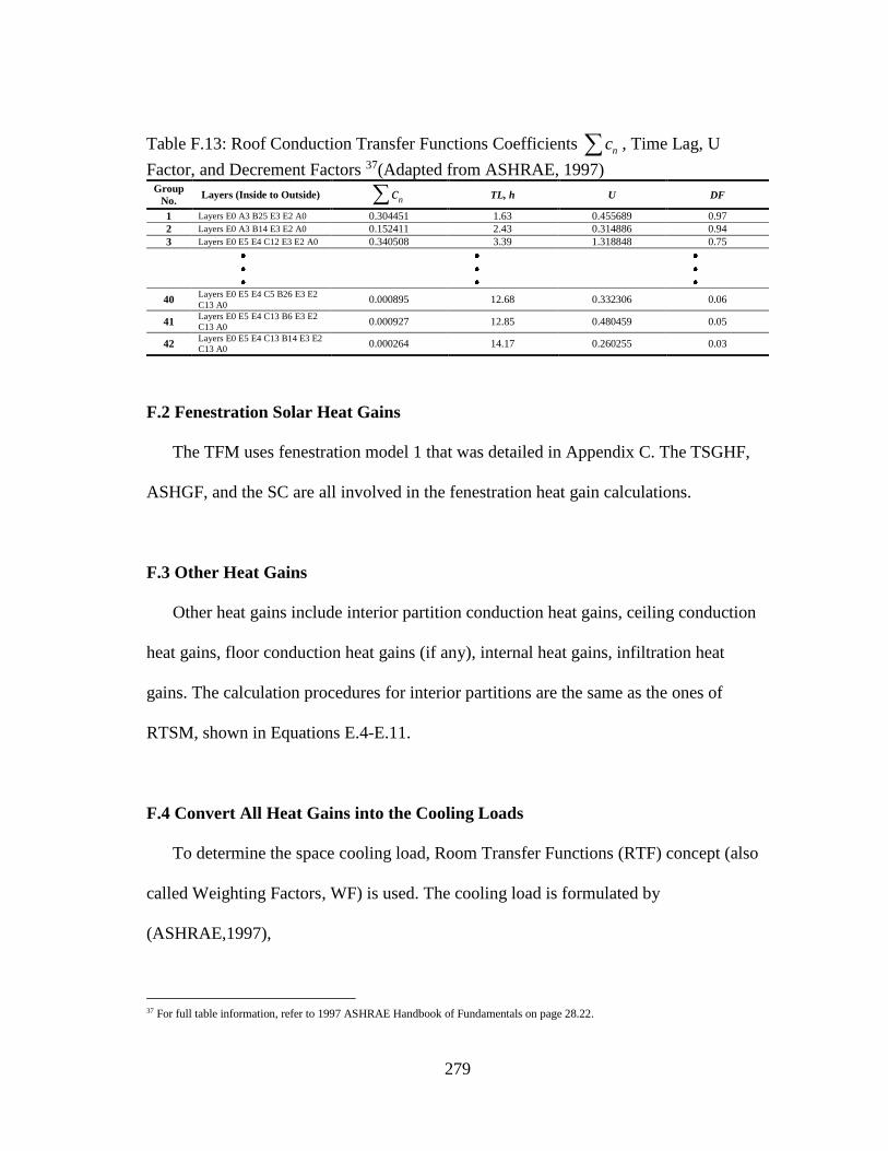
279
Table F.13: Roof Conduction Transfer Functions Coefficients nc , Time Lag, U
Factor, and Decrement Factors 37(Adapted from ASHRAE, 1997)
Group
No. Layers (Inside to Outside) nc TL, h U DF
1 Layers E0 A3 B25 E3 E2 A0 0.304451 1.63 0.455689 0.97
2 Layers E0 A3 B14 E3 E2 A0 0.152411 2.43 0.314886 0.94
3 Layers E0 E5 E4 C12 E3 E2 A0 0.340508 3.39 1.318848 0.75
40
Layers E0 E5 E4 C5 B26 E3 E2
C13 A0 0.000895 12.68 0.332306 0.06
41 Layers E0 E5 E4 C13 B6 E3 E2
C13 A0 0.000927 12.85 0.480459 0.05
42 Layers E0 E5 E4 C13 B14 E3 E2
C13 A0 0.000264 14.17 0.260255 0.03
F.2 Fenestration Solar Heat Gains
The TFM uses fenestration model 1 that was detailed in Appendix C. The TSGHF,
ASHGF, and the SC are all involved in the fenestration heat gain calculations.
F.3 Other Heat Gains
Other heat gains include interior partition conduction heat gains, ceiling conduction
heat gains, floor conduction heat gains (if any), internal heat gains, infiltration heat
gains. The calculation procedures for interior partitions are the same as the ones of
RTSM, shown in Equations E.4-E.11.
F.4 Convert All Heat Gains into the Cooling Loads
To determine the space cooling load, Room Transfer Functions (RTF) concept (also
called Weighting Factors, WF) is used. The cooling load is formulated by
(ASHRAE,1997),
37 For full table information, refer to 1997 ASHRAE Handbook of Fundamentals on page 28.22.
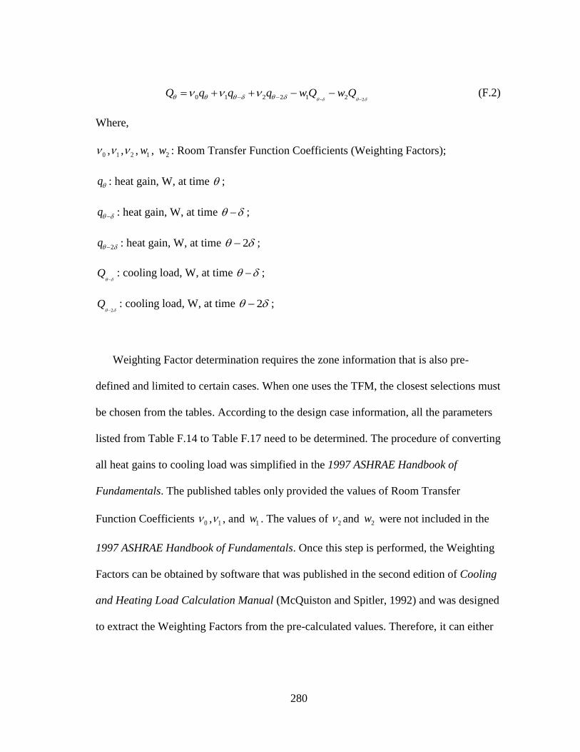
280
20 1 2 2 1 2 Q q q q w Q w Q (F.2)
Where,
0 , 1 , 2 , 1w , 2w : Room Transfer Function Coefficients (Weighting Factors);
q : heat gain, W, at time ;
q : heat gain, W, at time ;
2 q : heat gain, W, at time 2 ;
Q : cooling load, W, at time ;
2 Q : cooling load, W, at time 2 ;
Weighting Factor determination requires the zone information that is also pre-
defined and limited to certain cases. When one uses the TFM, the closest selections must
be chosen from the tables. According to the design case information, all the parameters
listed from Table F.14 to Table F.17 need to be determined. The procedure of converting
all heat gains to cooling load was simplified in the 1997 ASHRAE Handbook of
Fundamentals. The published tables only provided the values of Room Transfer
Function Coefficients 0 , 1 , and 1w . The values of 2 and 2w were not included in the
1997 ASHRAE Handbook of Fundamentals. Once this step is performed, the Weighting
Factors can be obtained by software that was published in the second edition of Cooling
and Heating Load Calculation Manual (McQuiston and Spitler, 1992) and was designed
to extract the Weighting Factors from the pre-calculated values. Therefore, it can either
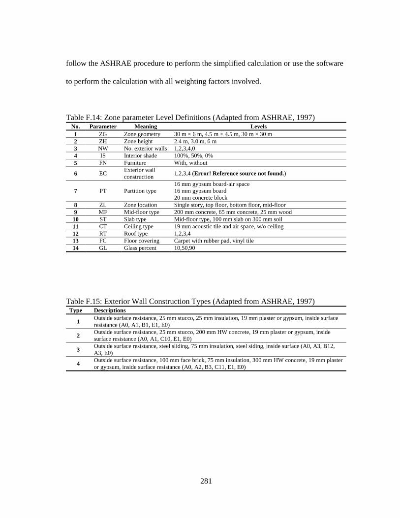
281
follow the ASHRAE procedure to perform the simplified calculation or use the software
to perform the calculation with all weighting factors involved.
Table F.14: Zone parameter Level Definitions (Adapted from ASHRAE, 1997) No. Parameter Meaning Levels
1 ZG Zone geometry 30 m × 6 m, 4.5 m × 4.5 m, 30 m × 30 m
2 ZH Zone height 2.4 m, 3.0 m, 6 m
3 NW No. exterior walls 1,2,3,4,0
4 IS Interior shade 100%, 50%, 0%
5 FN Furniture With, without
6 EC Exterior wall
construction 1,2,3,4 (Error! Reference source not found.)
7 PT Partition type
16 mm gypsum board-air space
16 mm gypsum board
20 mm concrete block
8 ZL Zone location Single story, top floor, bottom floor, mid-floor
9 MF Mid-floor type 200 mm concrete, 65 mm concrete, 25 mm wood
10 ST Slab type Mid-floor type, 100 mm slab on 300 mm soil
11 CT Ceiling type 19 mm acoustic tile and air space, w/o ceiling
12 RT Roof type 1,2,3,4
13 FC Floor covering Carpet with rubber pad, vinyl tile
14 GL Glass percent 10,50,90
Table F.15: Exterior Wall Construction Types (Adapted from ASHRAE, 1997) Type Descriptions
1 Outside surface resistance, 25 mm stucco, 25 mm insulation, 19 mm plaster or gypsum, inside surface
resistance (A0, A1, B1, E1, E0)
2 Outside surface resistance, 25 mm stucco, 200 mm HW concrete, 19 mm plaster or gypsum, inside
surface resistance (A0, A1, C10, E1, E0)
3 Outside surface resistance, steel sliding, 75 mm insulation, steel siding, inside surface (A0, A3, B12,
A3, E0)
4 Outside surface resistance, 100 mm face brick, 75 mm insulation, 300 mm HW concrete, 19 mm plaster
or gypsum, inside surface resistance (A0, A2, B3, C11, E1, E0)

282
Table F.16: Floor and Ceiling Types by Zone Location Parameter (Adapted from
ASHRAE, 1997) Zone Location Floor Ceiling
Single story Slab-on-grade Roof
Top floor Mid-floor Roof
Bottom floor Slab-on-grade Mid-floor
Mid-floor Mid-floor Mid-floor
Table F.17: Roof Construction Types (Adapted from ASHRAE, 1997) Type Descriptions
1 Outside surface resistance, 13 mm slag or stone, 10 mm felt membrane, 25 mm insulation, steel siding,
inside resistance (A0, E2, E3, B4, A3, E0)
2 Outside surface resistance, 13 mm slag or stone, 10 mm felt membrane, 150 mm LW concrete, inside
resistance (A0, E2, E3, C15, E0)
3 Outside surface resistance, 13 mm slag or stone, 10 mm felt membrane, 50 mm insulation, steel siding,
ceiling air space, acoustic tile, inside resistance (A0, E2, E3, B6, A3,E4, E5, E0)
4 Outside surface resistance, 13 mm slag or stone, 10 mm felt membrane, 200 mm LW concrete, ceiling
air space, acoustic tile, inside resistance (A0, E2, E3, C16,E4, E5, E0)
Figure F.2 shows the user interface of the software TFMTAB. By entering the
selected parameters, the program will return the Weighting Factors that can be used to
convert solar, conduction, and internal heat gains. Inserting all Weighting factors to
Equation (F.2) allows for the cooling loads to be determined. It is important to note that
several days of calculations with the exact same outside and inside conditions are needed
in order to achieve steady results since the cooling load equation involves the history
terms.

283
Figure F.2: Software user Interface
Figure F.3: Weighting Factor Results
284
APPENDIX G
TOTAL EQUIVALENT TEMPERATURE DIFFERENCE/TIME
AVERAGING METHOD (TETD/TA)
This section details the Total Equivalent Temperature Difference/Time Averaging
(TETD/TA) Method for peak cooling load calculations. Figure G.1 shows an overview
of this method (McQuiston and Spitler, 1992). Similar to the RTSM and the TFM, this
method uses the sol-air temperature concept. When calculating the conduction heat gains
through the walls and roofs, the Total Equivalent Temperature Difference (TETD) is
used. The fenestration model 1 is used for calculating the fenestration heat gains. Once
all heat gains are obtained, the radiative and convective portions are determined, using
the same procedure as RTSM. All the convective heat gains directly become the cooling
load. However, the radiative portions need a Time Averaging (TA) process to achieve
the final cooling load.
G.1 Exterior Conduction Heat Gains
The sol-air temperature can be calculated by Equation (B.30) using the solar
intensities detailed in Appendix B. The TETD is formulated by (ASHRAE, 1997),
,( )ea i e TL eaTETD t t DF t t (G.1)
where,

285
eat : daily average sol-air temperature, C;
it : indoor air temperature, C;
DF : decrement factor, dimensionless;
,e TLt : sol-air temperature at time lag (TL) hours ago, C.
Calculate hourly
and daily average
sol-air
temperatures for
each opaque
exterior surface
Calculate solar
intensities for
each hour for
each exterior
surface
Calculate Solar
Heat Gain Factors
(SHGF) for each
window
Calculate Total
Equivalent
Temperature
Differences
(TETD) for each
opaque exterior
surface
Determine wall
and roof types;
look up
decrement and
delay factors
Calculate solar
heat gain and
determine radiant
and convective
portions
Cooling loads for
conduction
through windows
are based on
UA∆T; assumed
all convective.
Determine
occupant, lighting
and equipment
loads; also
determine radiant
and convective
portions
Calculate heat
gains due to
conduction based
on TETD and UA
for each surface.
Determine
radiative and
convective
portions
All convective
gains are added
immediately to
cooling load.
All radiative
gains are time
averaged with
averaging period
selected by
designer. The
time average
determines the
cooling load for
each hour.
Sum cooling loads
Figure G.1: Overview of TETD Method (Adapted from McQuiston and Spitler, 1992)
And,

286
24
,
1
/ 24ea e i
i
t t
(G.2)
where,
,e it : sol-air temperature for hour i , C.
Following the same steps shown in Appendix F determines the wall and roof
numbers. Once the group numbers are determined, the decrement factor (DF) and time
lag (TL) can be obtained by using Table F.11 and Table F.13 for the walls and roofs,
respectively.
Then, the conduction heat gains through walls and roofs can be calculated by
(ASHRAE, 1997),
( )q UA TETD (G.3)
where,
U : overall heat transfer coefficient, W/m2-K;
A : surface area, m2.
G.2 Fenestration Solar Heat Gains
Fenestration model 1 is used in this method. However, in this method there is no
necessary to differentiate between the transmitted and absorbed solar heat gains, since
only total solar heat gain matters (see Appendix C).
287
G.3 Other Heat Gains
In this method, other heat gains include interior partition conduction heat gains,
ceiling conduction heat gains, floor conduction heat gains (if any), internal heat gains,
and infiltration heat gains. The calculation procedures for these other heat gains are the
same as the ones of RTSM, shown in Equations (E.4)-(E.11) in Appendix E.
G.4 Cooling Load by Time Averaging Process
Similar to the RTSM, after obtaining all types of heat gains, the convective and
radiative portions of heat gains need to be calculated using the most appropriate
convective and radiative proportions of total heat gains. Table G.1 shows the
percentages that were last updated by ASHRAE for TETD/TA Method. Later, when the
RTSM was introduced, the updated percentages for the convective and radiative portions
were recommended, shown in Table E.1 and Table E.2.
In the TETD/TA Method, all convective heat gains become cooling load directly,
while all radiative heat gains need the Time Averaging (TA) process. The purpose of this
is to account for the effects of the radiative heat gains from previous hours. However the
TA process time period needs to be selected by the designers. Unfortunately, this tends
to be a subjective decision that has a significant impact on the cooling load results. In
general, normal selection of time period for commercial construction is three hours. This
can vary from six to eight hours for a heavy construction (ASHRAE, 1993).
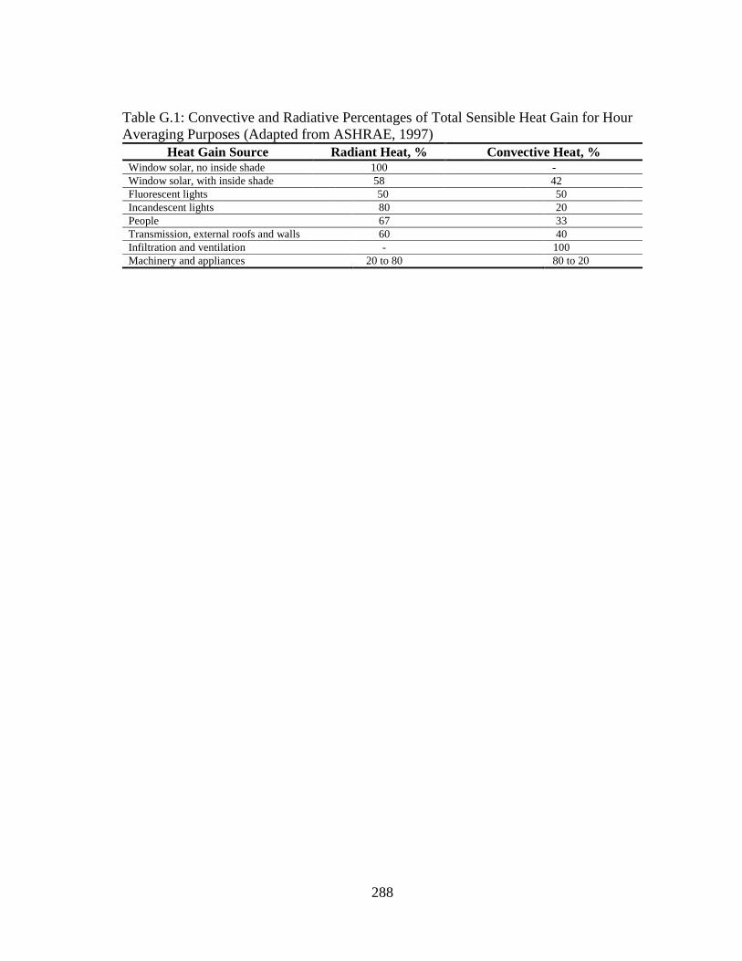
288
Table G.1: Convective and Radiative Percentages of Total Sensible Heat Gain for Hour
Averaging Purposes (Adapted from ASHRAE, 1997)
Heat Gain Source Radiant Heat, % Convective Heat, % Window solar, no inside shade 100 -
Window solar, with inside shade 58 42
Fluorescent lights 50 50
Incandescent lights 80 20
People 67 33
Transmission, external roofs and walls 60 40
Infiltration and ventilation - 100
Machinery and appliances 20 to 80 80 to 20
289
APPENDIX H
COOLING LOAD TEMPERATURE DIFFERENCE/SOLAR
COOLING LOAD/COOLING LOAD FACTOR METHOD
(CLTD/SCL/CLF)
This section discusses the procedure for peak cooling load calculation by the Cooling
Load Temperature Difference/Solar Cooling Load/Cooling Load Factor Method
(CLTD/SCL/CLF). As a one-step method, it relies on the CLTD, SCL, and CLF tables
that are generated based on Transfer Function Method (TFM). Different from TFM, the
principal material layers of walls and roofs are further regrouped. Varying on the months
and locations, the CLTD, SCL, and CLF tables need to be provided for each latitude and
month in order to perform calculations. The tabulated values are under the following
conditions (ASHRAE, 1997):
Dark surface;
Indoor temperature constant at 25.5 C;
Outdoor maximum temperature of 35 C, mean temperature 29.5 C;
Daily range of 11.6 C;
Clear sky on 21st day of the month;
Outside surface film resistance of 0.059 (m2-K/W);
No ceiling plenum air return system;
Inside surface resistance of 0.121 (m2-K/W)
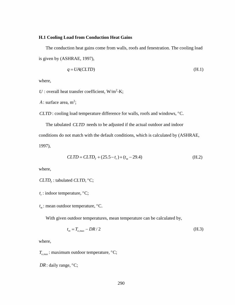
290
H.1 Cooling Load from Conduction Heat Gains
The conduction heat gains come from walls, roofs and fenestration. The cooling load
is given by (ASHRAE, 1997),
( )q UA CLTD (H.1)
where,
U : overall heat transfer coefficient, W/m2-K;
A : surface area, m2;
CLTD : cooling load temperature difference for walls, roofs and windows, C.
The tabulated CLTD needs to be adjusted if the actual outdoor and indoor
conditions do not match with the default conditions, which is calculated by (ASHRAE,
1997),
(25.5 ) ( 29.4)T r mCLTD CLTD t t (H.2)
where,
TCLTD : tabulated CLTD, C;
rt : indoor temperature, C;
mt : mean outdoor temperature, C.
With given outdoor temperatures, mean temperature can be calculated by,
,max / 2 m ot T DR (H.3)
where,
,maxoT : maximum outdoor temperature, C;
DR : daily range, C;

291
Similar to TFM, the wall and roof group numbers need to be determined first in
order to obtain tabulated CLTD values. The difference is that the wall and roof numbers
are regrouped once again. Compared to forty-one wall and forty-two roof numbers,
CLTD/SCL/CLF Method only has sixteen wall and ten roof numbers.
Table H.1 and Table H.2 are used to select proper wall and roof numbers. There are
fifteen and four principal materials for walls and roofs, respectively. The column can be
selected according to the principal material and the row number is up to R-value ranges
in the proper secondary material section for walls and proper suspended ceiling category
for roofs. The wall and roof numbers can be obtained by crosschecking the specific row
and column numbers.
Given by the wall and roof numbers of the design case, the tabulated CLTD values
can be obtained from Table H.3 and Table H.4. The wall CLTD values are generated for
a specific latitude and design month. Table H.3 shows an example table of tabulated
CLTD values for July and 40 N latitude. Only wall numbers 1 and 16 are presented in
this table. The full table with 16 wall numbers can be found in 1997 ASHRAE
Handbook of Fundamentals. The wall orientation finally determines the sets of tabulated
CLTD values that need to be used. Ten roof numbers are available for roof tabulated
CLTD value selections, shown in Table H.4. It is very important to note that the 24
hours represent the solar time instead of the local time. The cooling load can be time
shifted if the wrong time is used. Finally, the tabulated CLTD values for glass are shown
in Table H.5. Only one table is available for fenestration conduction cooling load
calculation by neglecting the latitude and month effects.

292
After adjusting the tabulated CLTD values by using Equation (H.2), the cooling load
from conduction heat gains can be calculated by using Equation (H.1). Not all the
tabulated CLTD values are available. A tool named “CLTDTAB”38 developed for the
Cooling and Heating Load Calculation Manual (McQuiston and Spitler, 1992) can be
used to generate the desired tables. Figure H.1 shows the user interface. By entering the
desired latitude and moth number, the tabulated CLTD values for walls and roofs are
generated, shown in Figure H.2. The program uses the linear interpolation for the
latitudes other than 24, 36, and 48 North. Even though the tables only reflect the 21st day
of each month, they are valid and suffice for the period of two weeks from the 21st
(McQuiston and Spitler, 1992).
Table H.1: Wall Group Numbers for Mass-In Case with Secondary Material of Stucco
and/or Plaster39 (Adapted from ASHRAE, 1997) R-Factor
(m2-K/W) Principal Wall Material
A1 A2 B7 B10 B9 C1 C2 C3 C4 C5 C6 C7 C8 C17 C18
0.0-0.35
0.35-0.44 5 5
0.44-0.53 5 3 2 5 6 5
0.53-0.62 5 4 2 2 5 6 6
0.62-0.70 5 4 2 3 6 6 10 4 6 5
0.70-0.84 6 5 2 4 6 6 11 5 10 10
0.84-0.97 6 5 2 4 6 6 11 5 10 10
0.97-1.14 6 5 2 5 10 7 12 5 11 10
1.14-1.36 6 5 4 5 11 7 16 10 11 11
1.36-1.59 6 5 4 5 11 7 10 11 11
1.59-1.89 6 5 4 5 11 7 10 11 4 11
1.89-2.24 6 5 4 5 11 11 10 11 4 11
2.24-2.64 10 10 4 5 11 11 10 11 9 12
2.64-3.08 10 10 5 5 11 11 11 12 10 16
3.08-3.52 11 10 5 9 11 11 15 16 10 16
3.52-4.05 11 10 9 9 16 11 15 16 10 16
4.05-4.76 16 15
38 CLTDTAB.EXE only generated the tables with IP unit. 39 This table only shows one kind of secondary material for walls with mass-in case. The full tables can be found in 1997 ASHRAE Handbook of Fundamentals on page 28.46.
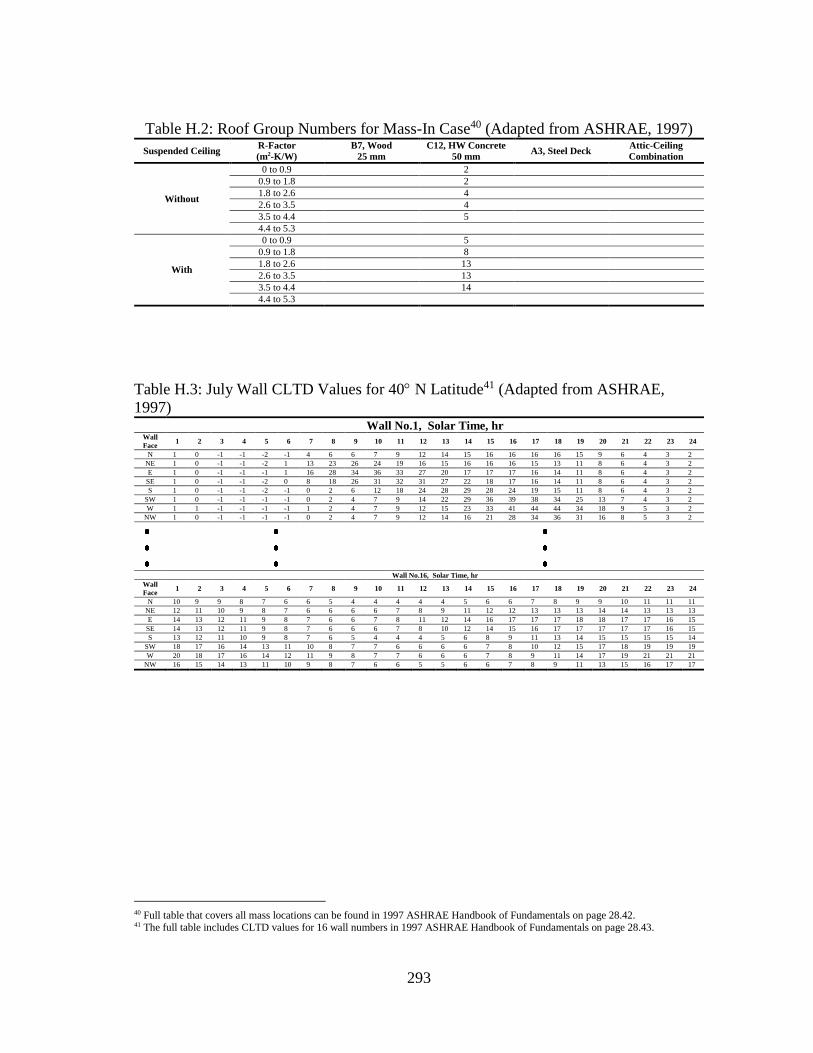
293
Table H.2: Roof Group Numbers for Mass-In Case40 (Adapted from ASHRAE, 1997)
Suspended Ceiling R-Factor
(m2-K/W)
B7, Wood
25 mm
C12, HW Concrete
50 mm A3, Steel Deck
Attic-Ceiling
Combination
Without
0 to 0.9 2
0.9 to 1.8 2
1.8 to 2.6 4
2.6 to 3.5 4
3.5 to 4.4 5
4.4 to 5.3
With
0 to 0.9 5
0.9 to 1.8 8
1.8 to 2.6 13
2.6 to 3.5 13
3.5 to 4.4 14
4.4 to 5.3
Table H.3: July Wall CLTD Values for 40 N Latitude41 (Adapted from ASHRAE,
1997)
Wall No.1, Solar Time, hr Wall
Face 1 2 3 4 5 6 7 8 9 10 11 12 13 14 15 16 17 18 19 20 21 22 23 24
N 1 0 -1 -1 -2 -1 4 6 6 7 9 12 14 15 16 16 16 16 15 9 6 4 3 2
NE 1 0 -1 -1 -2 1 13 23 26 24 19 16 15 16 16 16 15 13 11 8 6 4 3 2
E 1 0 -1 -1 -1 1 16 28 34 36 33 27 20 17 17 17 16 14 11 8 6 4 3 2
SE 1 0 -1 -1 -2 0 8 18 26 31 32 31 27 22 18 17 16 14 11 8 6 4 3 2
S 1 0 -1 -1 -2 -1 0 2 6 12 18 24 28 29 28 24 19 15 11 8 6 4 3 2
SW 1 0 -1 -1 -1 -1 0 2 4 7 9 14 22 29 36 39 38 34 25 13 7 4 3 2
W 1 1 -1 -1 -1 -1 1 2 4 7 9 12 15 23 33 41 44 44 34 18 9 5 3 2
NW 1 0 -1 -1 -1 -1 0 2 4 7 9 12 14 16 21 28 34 36 31 16 8 5 3 2
Wall No.16, Solar Time, hr
Wall
Face 1 2 3 4 5 6 7 8 9 10 11 12 13 14 15 16 17 18 19 20 21 22 23 24
N 10 9 9 8 7 6 6 5 4 4 4 4 4 5 6 6 7 8 9 9 10 11 11 11
NE 12 11 10 9 8 7 6 6 6 6 7 8 9 11 12 12 13 13 13 14 14 13 13 13
E 14 13 12 11 9 8 7 6 6 7 8 11 12 14 16 17 17 17 18 18 17 17 16 15
SE 14 13 12 11 9 8 7 6 6 6 7 8 10 12 14 15 16 17 17 17 17 17 16 15
S 13 12 11 10 9 8 7 6 5 4 4 4 5 6 8 9 11 13 14 15 15 15 15 14
SW 18 17 16 14 13 11 10 8 7 7 6 6 6 6 7 8 10 12 15 17 18 19 19 19
W 20 18 17 16 14 12 11 9 8 7 7 6 6 6 7 8 9 11 14 17 19 21 21 21
NW 16 15 14 13 11 10 9 8 7 6 6 5 5 6 6 7 8 9 11 13 15 16 17 17
40 Full table that covers all mass locations can be found in 1997 ASHRAE Handbook of Fundamentals on page 28.42. 41 The full table includes CLTD values for 16 wall numbers in 1997 ASHRAE Handbook of Fundamentals on page 28.43.
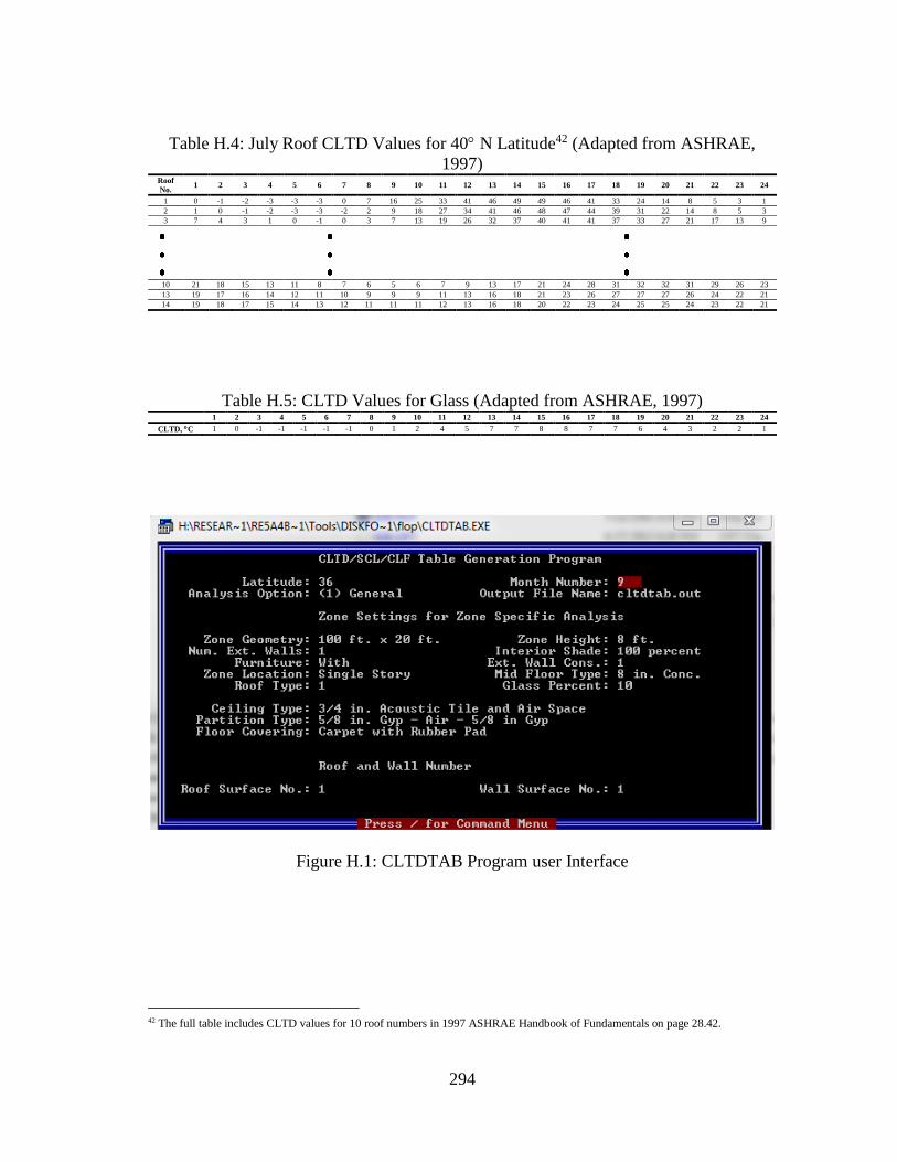
294
Table H.4: July Roof CLTD Values for 40 N Latitude42 (Adapted from ASHRAE,
1997) Roof
No. 1 2 3 4 5 6 7 8 9 10 11 12 13 14 15 16 17 18 19 20 21 22 23 24
1 0 -1 -2 -3 -3 -3 0 7 16 25 33 41 46 49 49 46 41 33 24 14 8 5 3 1
2 1 0 -1 -2 -3 -3 -2 2 9 18 27 34 41 46 48 47 44 39 31 22 14 8 5 3
3 7 4 3 1 0 -1 0 3 7 13 19 26 32 37 40 41 41 37 33 27 21 17 13 9
10 21 18 15 13 11 8 7 6 5 6 7 9 13 17 21 24 28 31 32 32 31 29 26 23
13 19 17 16 14 12 11 10 9 9 9 11 13 16 18 21 23 26 27 27 27 26 24 22 21
14 19 18 17 15 14 13 12 11 11 11 12 13 16 18 20 22 23 24 25 25 24 23 22 21
Table H.5: CLTD Values for Glass (Adapted from ASHRAE, 1997) 1 2 3 4 5 6 7 8 9 10 11 12 13 14 15 16 17 18 19 20 21 22 23 24
CLTD, C 1 0 -1 -1 -1 -1 -1 0 1 2 4 5 7 7 8 8 7 7 6 4 3 2 2 1
Figure H.1: CLTDTAB Program user Interface
42 The full table includes CLTD values for 10 roof numbers in 1997 ASHRAE Handbook of Fundamentals on page 28.42.
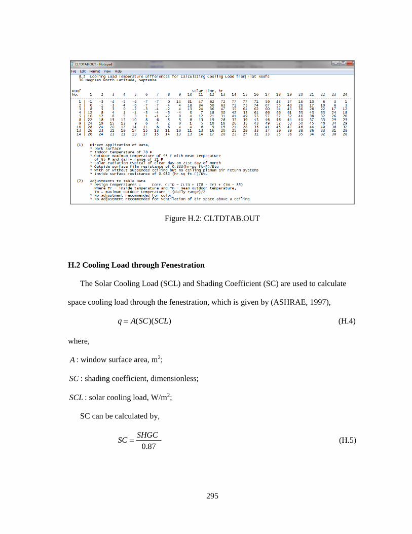
295
Figure H.2: CLTDTAB.OUT
H.2 Cooling Load through Fenestration
The Solar Cooling Load (SCL) and Shading Coefficient (SC) are used to calculate
space cooling load through the fenestration, which is given by (ASHRAE, 1997),
( )( )q A SC SCL (H.4)
where,
A : window surface area, m2;
SC : shading coefficient, dimensionless;
SCL : solar cooling load, W/m2;
SC can be calculated by,
0.87
SHGCSC (H.5)
296
where,
SHGC : normal solar heat gain coefficient of fenestration, dimensionless;
0.87 : normal solar heat gain coefficient for single-pane, double-strength, clear glass,
dimensionless;
Equation (H.4) uses SC instead of SHGC, which means the Fenestration Model 1 is
implemented in CLTD/SCL/CLF Method (see Appendix C).
Before using SCL tables, zone types need to first be determined. Four zone types are
available: zone type A, zone type B, zone type C, and zone type D. Four zone
parameters are involved to define a zone type: 1) number of exterior walls; 2) floor
covering; 3) partition type; 4) and inside shade. Similar to the TFM, the zone parameters
are limited and cannot cover all the actual design cases. Therefore, the users need to pick
the best fit. Table H.6 shows the zone types for glass solar, people & equipment, and
lights. Table H.7 shows the tabulated hourly SCL values for sunlit glass in July for 40
N Latitude. The hours still mean the solar hours, not the local hours. For a specific
latitude, CLTDTAB could be used to generate the desired tables, shown in Section H.1.

297
Table H.6: Zone Types for SCL and CLF Tables, Single-Story Building 43(Adapted from
ASHRAE, 1997)
Zone Parameters Zone Types Error Band No.
Walls
Floor
Covering
Partition
Type
Inside
Shade
Glass
Solar
People and
Equipment Lights Plus Minus
1 or 2 Carpet Gypsum Negligible A B B 9 2
1 or 2 Carpet Concrete
block Negligible B C C 9 0
4 Vinyl Gypsum Full B C C 11 6
4 Vinyl Gypsum Half to
None C C C 19 -1
Table H.7: July SCL for Sunlit Glass for 40 N Latitude 44 (Adapted from ASHRAE,
1997) Zone Type A , Solar Time, hr Glass
Face 1 2 3 4 5 6 7 8 9 10 11 12 13 14 15 16 17 18 19 20 21 22 23 24
N 0 0 0 0 3 79 85 88 101 110 120 126 126 123 113 98 98 113 38 19 9 3 3 0
NE 0 0 0 0 6 268 406 422 353 236 173 151 139 126 117 101 82 57 22 9 6 3 0 0
E 0 0 0 0 6 293 495 583 576 485 334 211 167 142 123 104 82 57 22 9 6 3 0 0
SE 0 0 0 0 3 148 299 413 473 473 413 306 198 154 129 107 85 57 22 9 6 3 0 0
S 0 0 0 0 0 28 54 79 129 202 268 306 302 265 198 132 98 63 25 13 6 3 0 0
SW 0 0 0 0 0 28 54 76 95 110 123 202 318 419 476 479 419 293 110 54 25 13 6 3
W 3 0 0 0 0 28 54 76 95 110 120 126 205 359 498 589 605 491 180 85 41 19 9 6
NW 3 0 0 0 0 28 54 76 95 110 120 126 126 158 265 381 450 410 145 69 35 16 9 3
Hor 0 0 0 0 0 76 217 378 532 665 759 810 816 772 684 554 394 221 91 44 22 9 6 3
H.3 Cooling Load from Partitions, Ceilings, and Floors
The calculations remain the same as Equation (E.4) in Appendix E.
H.4 Internal Cooling Load
For occupants,
, ( )s s perq q N CLF (H.6)
43 This table only contain a partial content. The full table can be found in 1997 ASHRAE Handbook of Fundamentals on page 28.49. 44 The full table includes SCL values for four zone types in 1997 ASHRAE Handbook of Fundamentals on page 28.50.
298
,l l perq q N (H.7)
where,
sq : occup1ant sensible heat gain, W;
lq : occupant latent heat gain, W;
,s perq : sensible heat gain per person W/person;
,l perq : latent heat gain per person, W/person;
N : number of occupants;
CLF : cooling load factor, dimensionless.
For lights,
( )el ul saq W F F CLF (H.8)
where,
elq : lighting heat gain, W;
W : total light wattage, W;
ulF : lighting use factor;
saF : lighting special allowance factor;
CLF : cooling load factor, dimensionless.
For powers,
( )em Fq P E CLF (H.9)

299
where,
P : motor power rating, W;
FE : efficiency factors and arrangements to suit circumstances;
CLF : cooling load factor, dimensionless;
For appliances,
( )s input U Rq q F F CLF (H.10)
where,
sq : sensible heat gain, W;
inputq : nameplate or rated energy input, W;
UF : usage factor;
RF : radiation factor;
CLF : cooling load factor, dimensionless.
Table H.8 shows an example CLFs table for people and unhood equipment. Similar
CLFs tables can be found in 1993 ASHRAE Handbook of Fundamentals for lights and
hooded equipment.
H.5 Cooling Load from Ventilation and Infiltration Air
The calculations remain the same as Equations (E. 10) and (E.11) in Appendix E.
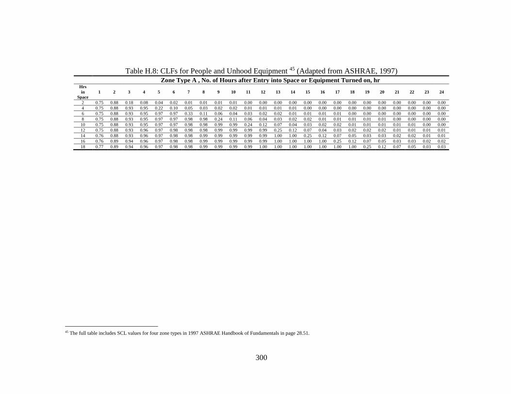
300
Table H.8: CLFs for People and Unhood Equipment 45 (Adapted from ASHRAE, 1997) Zone Type A , No. of Hours after Entry into Space or Equipment Turned on, hr Hrs
in
Space
1 2 3 4 5 6 7 8 9 10 11 12 13 14 15 16 17 18 19 20 21 22 23 24
2 0.75 0.88 0.18 0.08 0.04 0.02 0.01 0.01 0.01 0.01 0.00 0.00 0.00 0.00 0.00 0.00 0.00 0.00 0.00 0.00 0.00 0.00 0.00 0.00
4 0.75 0.88 0.93 0.95 0.22 0.10 0.05 0.03 0.02 0.02 0.01 0.01 0.01 0.01 0.00 0.00 0.00 0.00 0.00 0.00 0.00 0.00 0.00 0.00
6 0.75 0.88 0.93 0.95 0.97 0.97 0.33 0.11 0.06 0.04 0.03 0.02 0.02 0.01 0.01 0.01 0.01 0.00 0.00 0.00 0.00 0.00 0.00 0.00
8 0.75 0.88 0.93 0.95 0.97 0.97 0.98 0.98 0.24 0.11 0.06 0.04 0.03 0.02 0.02 0.01 0.01 0.01 0.01 0.01 0.00 0.00 0.00 0.00
10 0.75 0.88 0.93 0.95 0.97 0.97 0.98 0.98 0.99 0.99 0.24 0.12 0.07 0.04 0.03 0.02 0.02 0.01 0.01 0.01 0.01 0.01 0.00 0.00
12 0.75 0.88 0.93 0.96 0.97 0.98 0.98 0.98 0.99 0.99 0.99 0.99 0.25 0.12 0.07 0.04 0.03 0.02 0.02 0.02 0.01 0.01 0.01 0.01
14 0.76 0.88 0.93 0.96 0.97 0.98 0.98 0.99 0.99 0.99 0.99 0.99 1.00 1.00 0.25 0.12 0.07 0.05 0.03 0.03 0.02 0.02 0.01 0.01
16 0.76 0.89 0.94 0.96 0.97 0.98 0.98 0.99 0.99 0.99 0.99 0.99 1.00 1.00 1.00 1.00 0.25 0.12 0.07 0.05 0.03 0.03 0.02 0.02
18 0.77 0.89 0.94 0.96 0.97 0.98 0.98 0.99 0.99 0.99 0.99 1.00 1.00 1.00 1.00 1.00 1.00 1.00 0.25 0.12 0.07 0.05 0.03 0.03
45 The full table includes SCL values for four zone types in 1997 ASHRAE Handbook of Fundamentals in page 28.51.

301
APPENDIX I
SENSIBLE COOLING LOAD COMPARISON RESULTS FOR
ADDITIONAL CASE-STUDY COMPARISONS
This appendix presents the space sensible cooling load comparisons of the HBM, the
RTSM, the TFM, the TETD/TA Method, and the CLTD/SCL/CLF Method for both the
heavy-weight and light-weight building cases, shown in Figure I.1 to Figure I.30. Each
set of comparison includes the cooling load estimations from the five methods as well as
the cooling load difference respectively to the HBM and weather conditions. The test
cases are shown in Table I.1 and a detailed discussion of the results is provided in
Section 4.3.
Table I.1: Test Case Descriptions
Test
Case
No.
Glazing
Type
U-Value
(W/m2-K)
Normal
SHGC
Each Window
% to
Respective
Wall
Overall
WWR
Overall
WFR
South
Window
Area (m2)
West
Window
Area (m2)
Base Case
Single Pane Clear
4.65 0.86 58% 29% 96% 6.45 6.45
TC1 Single Pane
Clear 4.65 0.86
10% 5% 17% 1.12 1.12
TC2 30% 15% 50% 3.35 3.35
TC3 50% 25% 83% 5.58 5.58
TC4 Double Pane
Clear 2.73 0.76
10% 5% 17% 1.12 1.12
TC5 30% 15% 50% 3.35 3.35
TC6 50% 25% 83% 5.58 5.58
TC7 Double Pane
Low-e 1.99 0.70
10% 5% 17% 1.12 1.12
TC8 30% 15% 50% 3.35 3.35
TC9 50% 25% 83% 5.58 5.58
TC10 Triple Pane
Clear 1.76 0.68
10% 5% 17% 1.12 1.12
TC11 30% 15% 50% 3.35 3.35
TC12 50% 25% 83% 5.58 5.58
TC13 Triple Pane
Low-e 1.87 0.62
10% 5% 17% 1.12 1.12
TC14 30% 15% 50% 3.35 3.35
TC15 50% 25% 83% 5.58 5.58

302
-2000
-1000
0
1000
2000
3000
4000
5000
6000
12:00 AM 3:00 AM 6:00 AM 9:00 AM 12:00 PM 3:00 PM 6:00 PM 9:00 PM 12:00 AM
(W)
Time
Heavy Building Cooling Load
HBM
RTSM
TFM
TETD/TA
CLTD/SCL/CLF
-2000
-1000
0
1000
2000
3000
4000
5000
6000
12:00 AM 3:00 AM 6:00 AM 9:00 AM 12:00 PM 3:00 PM 6:00 PM 9:00 PM 12:00 AM
(W)
Time
Heavy Building Cooling Load Differences
RTSM-HBM
TFM-HBM
TETD/TA-HBM
CLTD/SCL/CLF-HBM
(b)(b)(b)(b)(b)
0
5
10
15
20
25
30
35
0
100
200
300
400
500
600
700
800
900
1000
12:00 AM 3:00 AM 6:00 AM 9:00 AM 12:00 PM 3:00 PM 6:00 PM 9:00 PM 12:00 AM Ou
tsid
e D
ry B
ulb
Te
mp
era
ture
(C
)W
ind
Sp
ee
d (
m/s
)
So
lar
Ra
dia
tio
n (
W/m
2)
Time
Weather Conditions
Global Solar Radiation(Measured) Global Solar Radiation (Clear Sky)Tdb WSTin
(c)
(a)
Figure I.1: TC 1 Space Sensible Cooling Load Comparisons for Heavy-Weight Building
Case
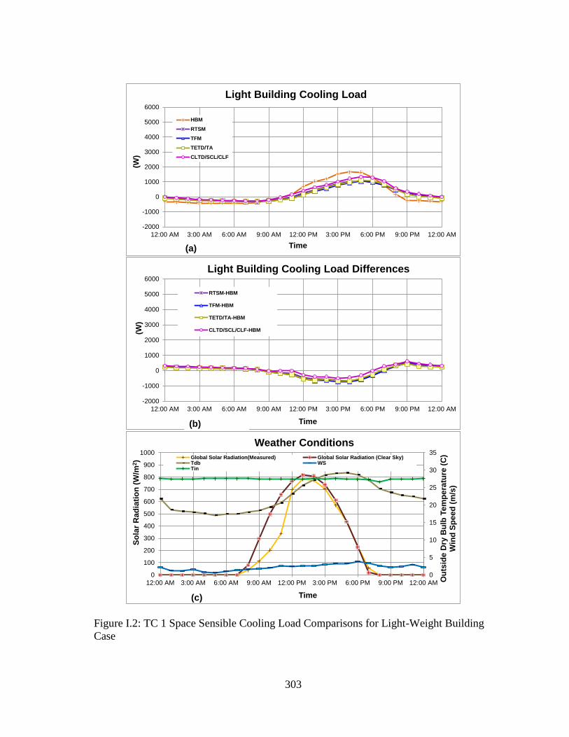
303
-2000
-1000
0
1000
2000
3000
4000
5000
6000
12:00 AM 3:00 AM 6:00 AM 9:00 AM 12:00 PM 3:00 PM 6:00 PM 9:00 PM 12:00 AM
(W)
Time
Light Building Cooling Load
HBM
RTSM
TFM
TETD/TA
CLTD/SCL/CLF
(a)
-2000
-1000
0
1000
2000
3000
4000
5000
6000
12:00 AM 3:00 AM 6:00 AM 9:00 AM 12:00 PM 3:00 PM 6:00 PM 9:00 PM 12:00 AM
(W)
Time
Light Building Cooling Load Differences
RTSM-HBM
TFM-HBM
TETD/TA-HBM
CLTD/SCL/CLF-HBM
(b)(b)(b)(b)(b)
0
5
10
15
20
25
30
35
0
100
200
300
400
500
600
700
800
900
1000
12:00 AM 3:00 AM 6:00 AM 9:00 AM 12:00 PM 3:00 PM 6:00 PM 9:00 PM 12:00 AM Ou
tsid
e D
ry B
ulb
Te
mp
era
ture
(C
)W
ind
Sp
ee
d (
m/s
)
So
lar
Ra
dia
tio
n (
W/m
2)
Time
Weather Conditions
Global Solar Radiation(Measured) Global Solar Radiation (Clear Sky)Tdb WSTin
(c)
Figure I.2: TC 1 Space Sensible Cooling Load Comparisons for Light-Weight Building
Case
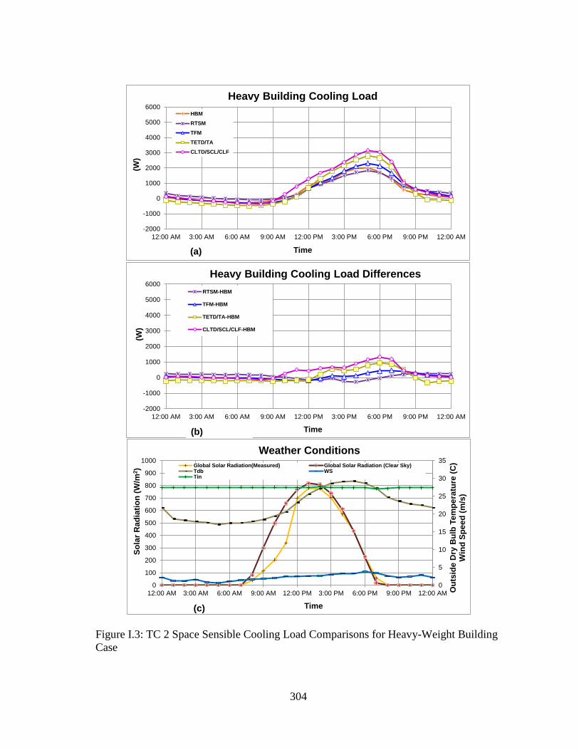
304
-2000
-1000
0
1000
2000
3000
4000
5000
6000
12:00 AM 3:00 AM 6:00 AM 9:00 AM 12:00 PM 3:00 PM 6:00 PM 9:00 PM 12:00 AM
(W)
Time
Heavy Building Cooling Load
HBM
RTSM
TFM
TETD/TA
CLTD/SCL/CLF
-2000
-1000
0
1000
2000
3000
4000
5000
6000
12:00 AM 3:00 AM 6:00 AM 9:00 AM 12:00 PM 3:00 PM 6:00 PM 9:00 PM 12:00 AM
(W)
Time
Heavy Building Cooling Load Differences
RTSM-HBM
TFM-HBM
TETD/TA-HBM
CLTD/SCL/CLF-HBM
(b)(b)(b)(b)(b)
0
5
10
15
20
25
30
35
0
100
200
300
400
500
600
700
800
900
1000
12:00 AM 3:00 AM 6:00 AM 9:00 AM 12:00 PM 3:00 PM 6:00 PM 9:00 PM 12:00 AM Ou
tsid
e D
ry B
ulb
Te
mp
era
ture
(C
)W
ind
Sp
ee
d (
m/s
)
So
lar
Ra
dia
tio
n (
W/m
2)
Time
Weather Conditions
Global Solar Radiation(Measured) Global Solar Radiation (Clear Sky)Tdb WSTin
(c)
(a)
Figure I.3: TC 2 Space Sensible Cooling Load Comparisons for Heavy-Weight Building
Case
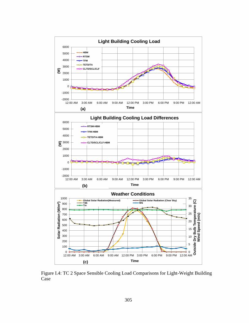
305
-2000
-1000
0
1000
2000
3000
4000
5000
6000
12:00 AM 3:00 AM 6:00 AM 9:00 AM 12:00 PM 3:00 PM 6:00 PM 9:00 PM 12:00 AM
(W)
Time
Light Building Cooling Load
HBM
RTSM
TFM
TETD/TA
CLTD/SCL/CLF
(a)
-2000
-1000
0
1000
2000
3000
4000
5000
6000
12:00 AM 3:00 AM 6:00 AM 9:00 AM 12:00 PM 3:00 PM 6:00 PM 9:00 PM 12:00 AM
(W)
Time
Light Building Cooling Load Differences
RTSM-HBM
TFM-HBM
TETD/TA-HBM
CLTD/SCL/CLF-HBM
(b)(b)(b)(b)(b)
0
5
10
15
20
25
30
35
0
100
200
300
400
500
600
700
800
900
1000
12:00 AM 3:00 AM 6:00 AM 9:00 AM 12:00 PM 3:00 PM 6:00 PM 9:00 PM 12:00 AM Ou
tsid
e D
ry B
ulb
Te
mp
era
ture
(C
)W
ind
Sp
ee
d (
m/s
)
So
lar
Ra
dia
tio
n (
W/m
2)
Time
Weather Conditions
Global Solar Radiation(Measured) Global Solar Radiation (Clear Sky)Tdb WSTin
(c)
Figure I.4: TC 2 Space Sensible Cooling Load Comparisons for Light-Weight Building
Case
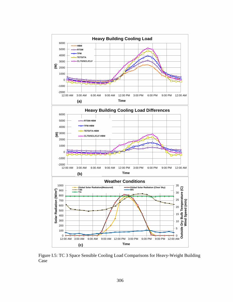
306
-2000
-1000
0
1000
2000
3000
4000
5000
6000
12:00 AM 3:00 AM 6:00 AM 9:00 AM 12:00 PM 3:00 PM 6:00 PM 9:00 PM 12:00 AM
(W)
Time
Heavy Building Cooling Load
HBM
RTSM
TFM
TETD/TA
CLTD/SCL/CLF
-2000
-1000
0
1000
2000
3000
4000
5000
6000
12:00 AM 3:00 AM 6:00 AM 9:00 AM 12:00 PM 3:00 PM 6:00 PM 9:00 PM 12:00 AM
(W)
Time
Heavy Building Cooling Load Differences
RTSM-HBM
TFM-HBM
TETD/TA-HBM
CLTD/SCL/CLF-HBM
(b)(b)(b)(b)(b)
0
5
10
15
20
25
30
35
0
100
200
300
400
500
600
700
800
900
1000
12:00 AM 3:00 AM 6:00 AM 9:00 AM 12:00 PM 3:00 PM 6:00 PM 9:00 PM 12:00 AM Ou
tsid
e D
ry B
ulb
Te
mp
era
ture
(C
)W
ind
Sp
ee
d (
m/s
)
So
lar
Rad
iati
on
(W
/m2)
Time
Weather Conditions
Global Solar Radiation(Measured) Global Solar Radiation (Clear Sky)Tdb WSTin
(c)
(a)
Figure I.5: TC 3 Space Sensible Cooling Load Comparisons for Heavy-Weight Building
Case
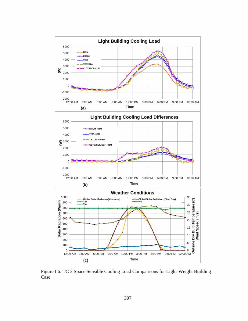
307
-2000
-1000
0
1000
2000
3000
4000
5000
6000
12:00 AM 3:00 AM 6:00 AM 9:00 AM 12:00 PM 3:00 PM 6:00 PM 9:00 PM 12:00 AM
(W)
Time
Light Building Cooling Load
HBM
RTSM
TFM
TETD/TA
CLTD/SCL/CLF
(a)
-2000
-1000
0
1000
2000
3000
4000
5000
6000
12:00 AM 3:00 AM 6:00 AM 9:00 AM 12:00 PM 3:00 PM 6:00 PM 9:00 PM 12:00 AM
(W)
Time
Light Building Cooling Load Differences
RTSM-HBM
TFM-HBM
TETD/TA-HBM
CLTD/SCL/CLF-HBM
(b)(b)(b)(b)(b)
0
5
10
15
20
25
30
35
0
100
200
300
400
500
600
700
800
900
1000
12:00 AM 3:00 AM 6:00 AM 9:00 AM 12:00 PM 3:00 PM 6:00 PM 9:00 PM 12:00 AM Ou
tsid
e D
ry B
ulb
Te
mp
era
ture
(C
)W
ind
Sp
ee
d (
m/s
)
So
lar
Ra
dia
tio
n (
W/m
2)
Time
Weather Conditions
Global Solar Radiation(Measured) Global Solar Radiation (Clear Sky)Tdb WSTin
(c)
Figure I.6: TC 3 Space Sensible Cooling Load Comparisons for Light-Weight Building
Case

308
-2000
-1000
0
1000
2000
3000
4000
5000
6000
12:00 AM 3:00 AM 6:00 AM 9:00 AM 12:00 PM 3:00 PM 6:00 PM 9:00 PM 12:00 AM
(W)
Time
Heavy Building Cooling Load
HBM
RTSM
TFM
TETD/TA
CLTD/SCL/CLF
-2000
-1000
0
1000
2000
3000
4000
5000
6000
12:00 AM 3:00 AM 6:00 AM 9:00 AM 12:00 PM 3:00 PM 6:00 PM 9:00 PM 12:00 AM
(W)
Time
Heavy Building Cooling Load Differences
RTSM-HBM
TFM-HBM
TETD/TA-HBM
CLTD/SCL/CLF-HBM
(b)(b)(b)(b)(b)
0
5
10
15
20
25
30
35
0
100
200
300
400
500
600
700
800
900
1000
12:00 AM 3:00 AM 6:00 AM 9:00 AM 12:00 PM 3:00 PM 6:00 PM 9:00 PM 12:00 AM Ou
tsid
e D
ry B
ulb
Te
mp
era
ture
(C
)W
ind
Sp
ee
d (
m/s
)
So
lar
Rad
iati
on
(W
/m2)
Time
Weather Conditions
Global Solar Radiation(Measured) Global Solar Radiation (Clear Sky)Tdb WSTin
(c)
(a)
Figure I.7: TC 4 Space Sensible Cooling Load Comparisons for Heavy-Weight Building
Case

309
-2000
-1000
0
1000
2000
3000
4000
5000
6000
12:00 AM 3:00 AM 6:00 AM 9:00 AM 12:00 PM 3:00 PM 6:00 PM 9:00 PM 12:00 AM
(W)
Time
Light Building Cooling Load
HBM
RTSM
TFM
TETD/TA
CLTD/SCL/CLF
(a)
-2000
-1000
0
1000
2000
3000
4000
5000
6000
12:00 AM 3:00 AM 6:00 AM 9:00 AM 12:00 PM 3:00 PM 6:00 PM 9:00 PM 12:00 AM
(W)
Time
Light Building Cooling Load Differences
RTSM-HBM
TFM-HBM
TETD/TA-HBM
CLTD/SCL/CLF-HBM
(b)(b)(b)(b)(b)
0
5
10
15
20
25
30
35
0
100
200
300
400
500
600
700
800
900
1000
12:00 AM 3:00 AM 6:00 AM 9:00 AM 12:00 PM 3:00 PM 6:00 PM 9:00 PM 12:00 AM Ou
tsid
e D
ry B
ulb
Te
mp
era
ture
(C
)W
ind
Sp
ee
d (
m/s
)
So
lar
Ra
dia
tio
n (
W/m
2)
Time
Weather Conditions
Global Solar Radiation(Measured) Global Solar Radiation (Clear Sky)Tdb WSTin
(c)
Figure I.8: TC 4 Space Sensible Cooling Load Comparisons for Light-Weight Building
Case
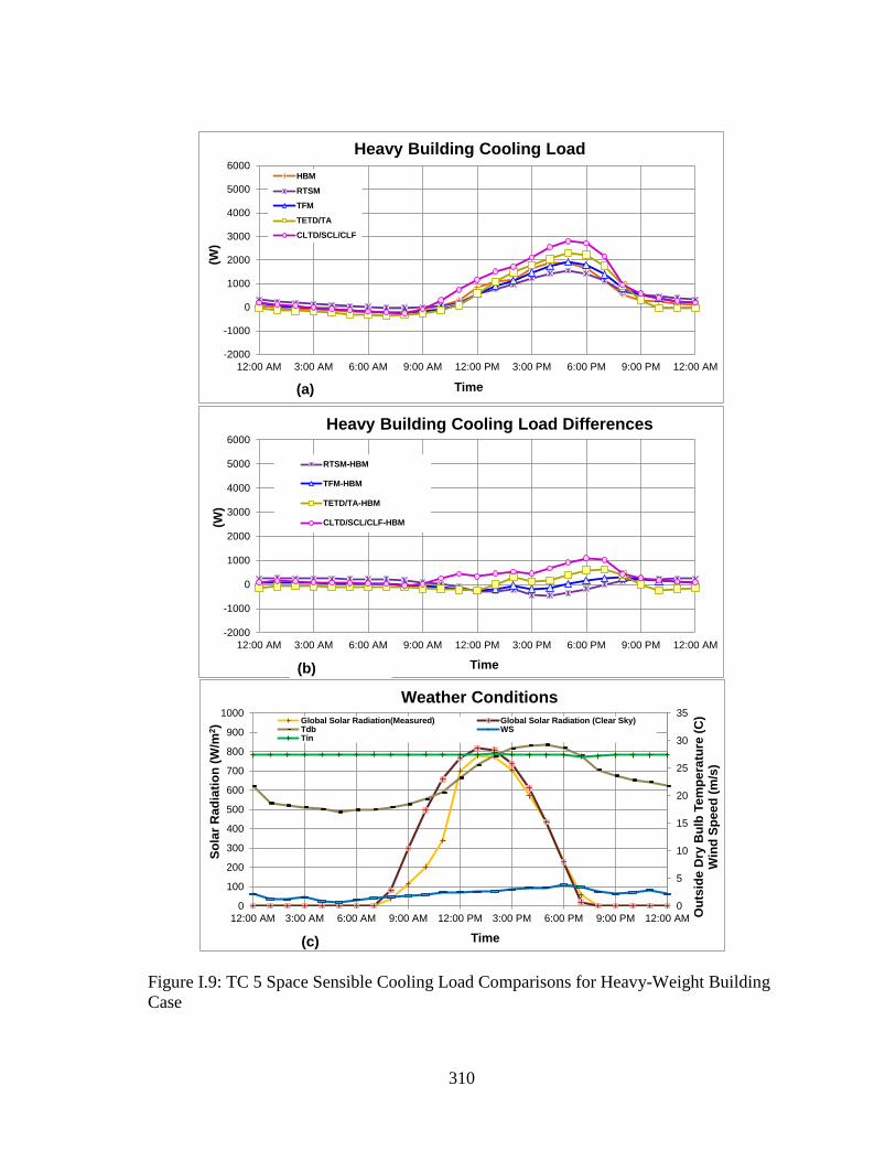
310
-2000
-1000
0
1000
2000
3000
4000
5000
6000
12:00 AM 3:00 AM 6:00 AM 9:00 AM 12:00 PM 3:00 PM 6:00 PM 9:00 PM 12:00 AM
(W)
Time
Heavy Building Cooling Load
HBM
RTSM
TFM
TETD/TA
CLTD/SCL/CLF
-2000
-1000
0
1000
2000
3000
4000
5000
6000
12:00 AM 3:00 AM 6:00 AM 9:00 AM 12:00 PM 3:00 PM 6:00 PM 9:00 PM 12:00 AM
(W)
Time
Heavy Building Cooling Load Differences
RTSM-HBM
TFM-HBM
TETD/TA-HBM
CLTD/SCL/CLF-HBM
(b)(b)(b)(b)(b)
0
5
10
15
20
25
30
35
0
100
200
300
400
500
600
700
800
900
1000
12:00 AM 3:00 AM 6:00 AM 9:00 AM 12:00 PM 3:00 PM 6:00 PM 9:00 PM 12:00 AM Ou
tsid
e D
ry B
ulb
Te
mp
era
ture
(C
)W
ind
Sp
ee
d (
m/s
)
So
lar
Rad
iati
on
(W
/m2)
Time
Weather Conditions
Global Solar Radiation(Measured) Global Solar Radiation (Clear Sky)Tdb WSTin
(c)
(a)
Figure I.9: TC 5 Space Sensible Cooling Load Comparisons for Heavy-Weight Building
Case
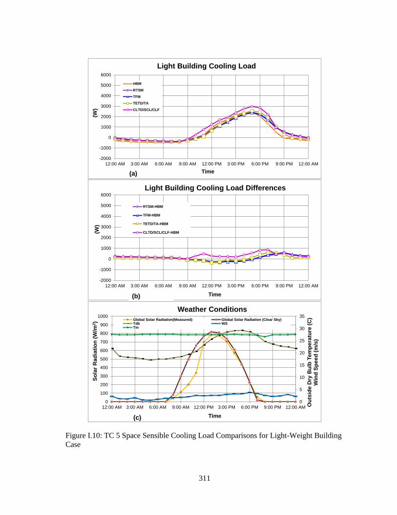
311
-2000
-1000
0
1000
2000
3000
4000
5000
6000
12:00 AM 3:00 AM 6:00 AM 9:00 AM 12:00 PM 3:00 PM 6:00 PM 9:00 PM 12:00 AM
(W)
Time
Light Building Cooling Load
HBM
RTSM
TFM
TETD/TA
CLTD/SCL/CLF
(a)
-2000
-1000
0
1000
2000
3000
4000
5000
6000
12:00 AM 3:00 AM 6:00 AM 9:00 AM 12:00 PM 3:00 PM 6:00 PM 9:00 PM 12:00 AM
(W)
Time
Light Building Cooling Load Differences
RTSM-HBM
TFM-HBM
TETD/TA-HBM
CLTD/SCL/CLF-HBM
(b)(b)(b)(b)(b)
0
5
10
15
20
25
30
35
0
100
200
300
400
500
600
700
800
900
1000
12:00 AM 3:00 AM 6:00 AM 9:00 AM 12:00 PM 3:00 PM 6:00 PM 9:00 PM 12:00 AM Ou
tsid
e D
ry B
ulb
Te
mp
era
ture
(C
)W
ind
Sp
ee
d (
m/s
)
So
lar
Ra
dia
tio
n (
W/m
2)
Time
Weather Conditions
Global Solar Radiation(Measured) Global Solar Radiation (Clear Sky)Tdb WSTin
(c)
Figure I.10: TC 5 Space Sensible Cooling Load Comparisons for Light-Weight Building
Case
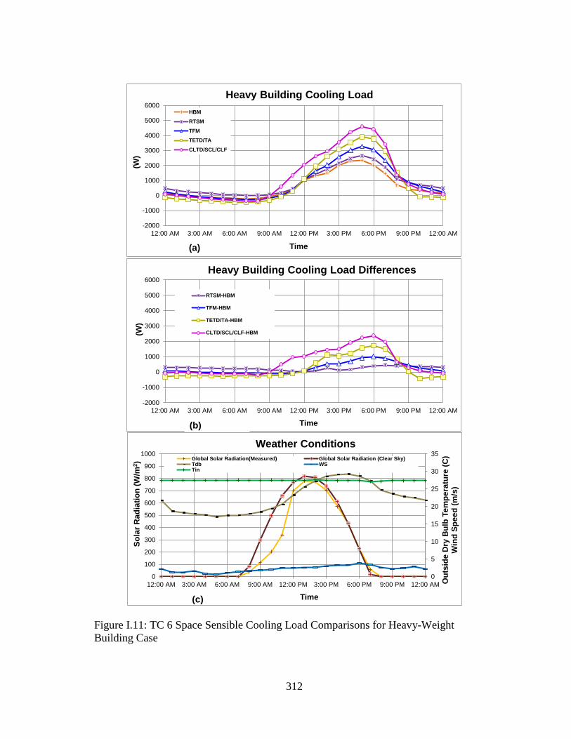
312
-2000
-1000
0
1000
2000
3000
4000
5000
6000
12:00 AM 3:00 AM 6:00 AM 9:00 AM 12:00 PM 3:00 PM 6:00 PM 9:00 PM 12:00 AM
(W)
Time
Heavy Building Cooling Load
HBM
RTSM
TFM
TETD/TA
CLTD/SCL/CLF
-2000
-1000
0
1000
2000
3000
4000
5000
6000
12:00 AM 3:00 AM 6:00 AM 9:00 AM 12:00 PM 3:00 PM 6:00 PM 9:00 PM 12:00 AM
(W)
Time
Heavy Building Cooling Load Differences
RTSM-HBM
TFM-HBM
TETD/TA-HBM
CLTD/SCL/CLF-HBM
(b)(b)(b)(b)(b)
0
5
10
15
20
25
30
35
0
100
200
300
400
500
600
700
800
900
1000
12:00 AM 3:00 AM 6:00 AM 9:00 AM 12:00 PM 3:00 PM 6:00 PM 9:00 PM 12:00 AM Ou
tsid
e D
ry B
ulb
Te
mp
era
ture
(C
)W
ind
Sp
ee
d (
m/s
)
So
lar
Rad
iati
on
(W
/m2)
Time
Weather Conditions
Global Solar Radiation(Measured) Global Solar Radiation (Clear Sky)Tdb WSTin
(c)
(a)
Figure I.11: TC 6 Space Sensible Cooling Load Comparisons for Heavy-Weight
Building Case

313
-2000
-1000
0
1000
2000
3000
4000
5000
6000
12:00 AM 3:00 AM 6:00 AM 9:00 AM 12:00 PM 3:00 PM 6:00 PM 9:00 PM 12:00 AM
(W)
Time
Light Building Cooling Load
HBM
RTSM
TFM
TETD/TA
CLTD/SCL/CLF
(a)
-2000
-1000
0
1000
2000
3000
4000
5000
6000
12:00 AM 3:00 AM 6:00 AM 9:00 AM 12:00 PM 3:00 PM 6:00 PM 9:00 PM 12:00 AM
(W)
Time
Light Building Cooling Load Differences
RTSM-HBM
TFM-HBM
TETD/TA-HBM
CLTD/SCL/CLF-HBM
(b)(b)(b)(b)(b)
0
5
10
15
20
25
30
35
0
100
200
300
400
500
600
700
800
900
1000
12:00 AM 3:00 AM 6:00 AM 9:00 AM 12:00 PM 3:00 PM 6:00 PM 9:00 PM 12:00 AM Ou
tsid
e D
ry B
ulb
Te
mp
era
ture
(C
)W
ind
Sp
ee
d (
m/s
)
So
lar
Ra
dia
tio
n (
W/m
2)
Time
Weather Conditions
Global Solar Radiation(Measured) Global Solar Radiation (Clear Sky)Tdb WSTin
(c)
Figure I.12: TC 6 Space Sensible Cooling Load Comparisons for Light-Weight Building
Case

314
-2000
-1000
0
1000
2000
3000
4000
5000
6000
12:00 AM 3:00 AM 6:00 AM 9:00 AM 12:00 PM 3:00 PM 6:00 PM 9:00 PM 12:00 AM
(W)
Time
Heavy Building Cooling Load
HBM
RTSM
TFM
TETD/TA
CLTD/SCL/CLF
-2000
-1000
0
1000
2000
3000
4000
5000
6000
12:00 AM 3:00 AM 6:00 AM 9:00 AM 12:00 PM 3:00 PM 6:00 PM 9:00 PM 12:00 AM
(W)
Time
Heavy Building Cooling Load Differences
RTSM-HBM
TFM-HBM
TETD/TA-HBM
CLTD/SCL/CLF-HBM
(b)(b)(b)(b)(b)
0
5
10
15
20
25
30
35
0
100
200
300
400
500
600
700
800
900
1000
12:00 AM 3:00 AM 6:00 AM 9:00 AM 12:00 PM 3:00 PM 6:00 PM 9:00 PM 12:00 AM Ou
tsid
e D
ry B
ulb
Te
mp
era
ture
(C
)W
ind
Sp
ee
d (
m/s
)
So
lar
Rad
iati
on
(W
/m2)
Time
Weather Conditions
Global Solar Radiation(Measured) Global Solar Radiation (Clear Sky)Tdb WSTin
(c)
(a)
Figure I.13: TC 7 Space Sensible Cooling Load Comparisons for Heavy-Weight
Building Case
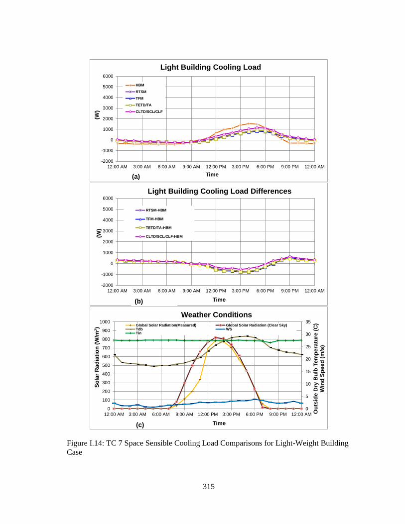
315
-2000
-1000
0
1000
2000
3000
4000
5000
6000
12:00 AM 3:00 AM 6:00 AM 9:00 AM 12:00 PM 3:00 PM 6:00 PM 9:00 PM 12:00 AM
(W)
Time
Light Building Cooling Load
HBM
RTSM
TFM
TETD/TA
CLTD/SCL/CLF
(a)
-2000
-1000
0
1000
2000
3000
4000
5000
6000
12:00 AM 3:00 AM 6:00 AM 9:00 AM 12:00 PM 3:00 PM 6:00 PM 9:00 PM 12:00 AM
(W)
Time
Light Building Cooling Load Differences
RTSM-HBM
TFM-HBM
TETD/TA-HBM
CLTD/SCL/CLF-HBM
(b)(b)(b)(b)(b)
0
5
10
15
20
25
30
35
0
100
200
300
400
500
600
700
800
900
1000
12:00 AM 3:00 AM 6:00 AM 9:00 AM 12:00 PM 3:00 PM 6:00 PM 9:00 PM 12:00 AM Ou
tsid
e D
ry B
ulb
Te
mp
era
ture
(C
)W
ind
Sp
ee
d (
m/s
)
So
lar
Ra
dia
tio
n (
W/m
2)
Time
Weather Conditions
Global Solar Radiation(Measured) Global Solar Radiation (Clear Sky)Tdb WSTin
(c)
Figure I.14: TC 7 Space Sensible Cooling Load Comparisons for Light-Weight Building
Case
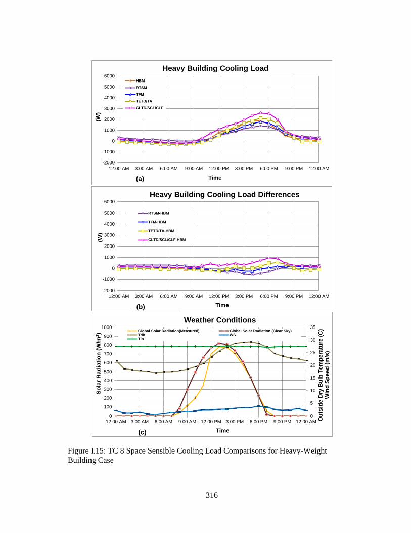
316
-2000
-1000
0
1000
2000
3000
4000
5000
6000
12:00 AM 3:00 AM 6:00 AM 9:00 AM 12:00 PM 3:00 PM 6:00 PM 9:00 PM 12:00 AM
(W)
Time
Heavy Building Cooling Load
HBM
RTSM
TFM
TETD/TA
CLTD/SCL/CLF
-2000
-1000
0
1000
2000
3000
4000
5000
6000
12:00 AM 3:00 AM 6:00 AM 9:00 AM 12:00 PM 3:00 PM 6:00 PM 9:00 PM 12:00 AM
(W)
Time
Heavy Building Cooling Load Differences
RTSM-HBM
TFM-HBM
TETD/TA-HBM
CLTD/SCL/CLF-HBM
(b)(b)(b)(b)(b)
0
5
10
15
20
25
30
35
0
100
200
300
400
500
600
700
800
900
1000
12:00 AM 3:00 AM 6:00 AM 9:00 AM 12:00 PM 3:00 PM 6:00 PM 9:00 PM 12:00 AM Ou
tsid
e D
ry B
ulb
Te
mp
era
ture
(C
)W
ind
Sp
ee
d (
m/s
)
So
lar
Rad
iati
on
(W
/m2)
Time
Weather Conditions
Global Solar Radiation(Measured) Global Solar Radiation (Clear Sky)Tdb WSTin
(c)
(a)
Figure I.15: TC 8 Space Sensible Cooling Load Comparisons for Heavy-Weight
Building Case
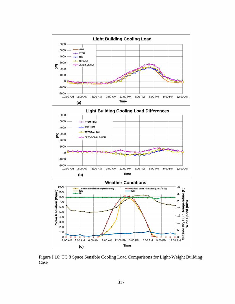
317
-2000
-1000
0
1000
2000
3000
4000
5000
6000
12:00 AM 3:00 AM 6:00 AM 9:00 AM 12:00 PM 3:00 PM 6:00 PM 9:00 PM 12:00 AM
(W)
Time
Light Building Cooling Load
HBM
RTSM
TFM
TETD/TA
CLTD/SCL/CLF
(a)
-2000
-1000
0
1000
2000
3000
4000
5000
6000
12:00 AM 3:00 AM 6:00 AM 9:00 AM 12:00 PM 3:00 PM 6:00 PM 9:00 PM 12:00 AM
(W)
Time
Light Building Cooling Load Differences
RTSM-HBM
TFM-HBM
TETD/TA-HBM
CLTD/SCL/CLF-HBM
(b)(b)(b)(b)(b)
0
5
10
15
20
25
30
35
0
100
200
300
400
500
600
700
800
900
1000
12:00 AM 3:00 AM 6:00 AM 9:00 AM 12:00 PM 3:00 PM 6:00 PM 9:00 PM 12:00 AM Ou
tsid
e D
ry B
ulb
Te
mp
era
ture
(C
)W
ind
Sp
ee
d (
m/s
)
So
lar
Ra
dia
tio
n (
W/m
2)
Time
Weather Conditions
Global Solar Radiation(Measured) Global Solar Radiation (Clear Sky)Tdb WSTin
(c)
Figure I.16: TC 8 Space Sensible Cooling Load Comparisons for Light-Weight Building
Case
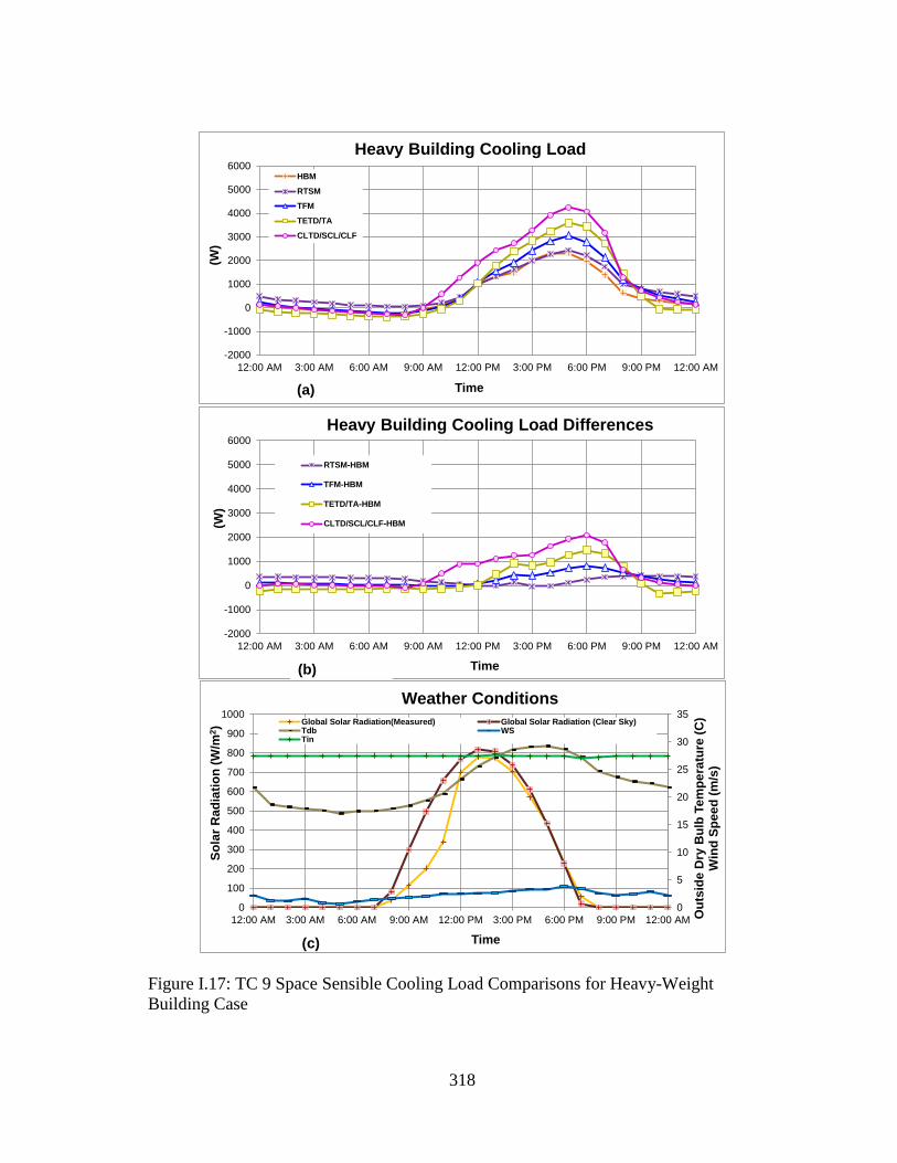
318
-2000
-1000
0
1000
2000
3000
4000
5000
6000
12:00 AM 3:00 AM 6:00 AM 9:00 AM 12:00 PM 3:00 PM 6:00 PM 9:00 PM 12:00 AM
(W)
Time
Heavy Building Cooling Load
HBM
RTSM
TFM
TETD/TA
CLTD/SCL/CLF
-2000
-1000
0
1000
2000
3000
4000
5000
6000
12:00 AM 3:00 AM 6:00 AM 9:00 AM 12:00 PM 3:00 PM 6:00 PM 9:00 PM 12:00 AM
(W)
Time
Heavy Building Cooling Load Differences
RTSM-HBM
TFM-HBM
TETD/TA-HBM
CLTD/SCL/CLF-HBM
(b)(b)(b)(b)(b)
0
5
10
15
20
25
30
35
0
100
200
300
400
500
600
700
800
900
1000
12:00 AM 3:00 AM 6:00 AM 9:00 AM 12:00 PM 3:00 PM 6:00 PM 9:00 PM 12:00 AM Ou
tsid
e D
ry B
ulb
Te
mp
era
ture
(C
)W
ind
Sp
ee
d (
m/s
)
So
lar
Rad
iati
on
(W
/m2)
Time
Weather Conditions
Global Solar Radiation(Measured) Global Solar Radiation (Clear Sky)Tdb WSTin
(c)
(a)
Figure I.17: TC 9 Space Sensible Cooling Load Comparisons for Heavy-Weight
Building Case

319
-2000
-1000
0
1000
2000
3000
4000
5000
6000
12:00 AM 3:00 AM 6:00 AM 9:00 AM 12:00 PM 3:00 PM 6:00 PM 9:00 PM 12:00 AM
(W)
Time
Light Building Cooling Load
HBM
RTSM
TFM
TETD/TA
CLTD/SCL/CLF
(a)
-2000
-1000
0
1000
2000
3000
4000
5000
6000
12:00 AM 3:00 AM 6:00 AM 9:00 AM 12:00 PM 3:00 PM 6:00 PM 9:00 PM 12:00 AM
(W)
Time
Light Building Cooling Load Differences
RTSM-HBM
TFM-HBM
TETD/TA-HBM
CLTD/SCL/CLF-HBM
(b)(b)(b)(b)(b)
0
5
10
15
20
25
30
35
0
100
200
300
400
500
600
700
800
900
1000
12:00 AM 3:00 AM 6:00 AM 9:00 AM 12:00 PM 3:00 PM 6:00 PM 9:00 PM 12:00 AM Ou
tsid
e D
ry B
ulb
Te
mp
era
ture
(C
)W
ind
Sp
ee
d (
m/s
)
So
lar
Ra
dia
tio
n (
W/m
2)
Time
Weather Conditions
Global Solar Radiation(Measured) Global Solar Radiation (Clear Sky)Tdb WSTin
(c)
Figure I.18: TC 9 Space Sensible Cooling Load Comparisons for Light-Weight Building
Case
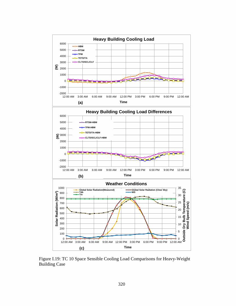
320
-2000
-1000
0
1000
2000
3000
4000
5000
6000
12:00 AM 3:00 AM 6:00 AM 9:00 AM 12:00 PM 3:00 PM 6:00 PM 9:00 PM 12:00 AM
(W)
Time
Heavy Building Cooling Load
HBM
RTSM
TFM
TETD/TA
CLTD/SCL/CLF
-2000
-1000
0
1000
2000
3000
4000
5000
6000
12:00 AM 3:00 AM 6:00 AM 9:00 AM 12:00 PM 3:00 PM 6:00 PM 9:00 PM 12:00 AM
(W)
Time
Heavy Building Cooling Load Differences
RTSM-HBM
TFM-HBM
TETD/TA-HBM
CLTD/SCL/CLF-HBM
(b)(b)(b)(b)(b)
0
5
10
15
20
25
30
35
0
100
200
300
400
500
600
700
800
900
1000
12:00 AM 3:00 AM 6:00 AM 9:00 AM 12:00 PM 3:00 PM 6:00 PM 9:00 PM 12:00 AM Ou
tsid
e D
ry B
ulb
Te
mp
era
ture
(C
)W
ind
Sp
ee
d (
m/s
)
So
lar
Rad
iati
on
(W
/m2)
Time
Weather Conditions
Global Solar Radiation(Measured) Global Solar Radiation (Clear Sky)Tdb WSTin
(c)
(a)
Figure I.19: TC 10 Space Sensible Cooling Load Comparisons for Heavy-Weight
Building Case
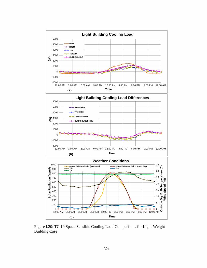
321
-2000
-1000
0
1000
2000
3000
4000
5000
6000
12:00 AM 3:00 AM 6:00 AM 9:00 AM 12:00 PM 3:00 PM 6:00 PM 9:00 PM 12:00 AM
(W)
Time
Light Building Cooling Load
HBM
RTSM
TFM
TETD/TA
CLTD/SCL/CLF
(a)
-2000
-1000
0
1000
2000
3000
4000
5000
6000
12:00 AM 3:00 AM 6:00 AM 9:00 AM 12:00 PM 3:00 PM 6:00 PM 9:00 PM 12:00 AM
(W)
Time
Light Building Cooling Load Differences
RTSM-HBM
TFM-HBM
TETD/TA-HBM
CLTD/SCL/CLF-HBM
(b)(b)(b)(b)(b)
0
5
10
15
20
25
30
35
0
100
200
300
400
500
600
700
800
900
1000
12:00 AM 3:00 AM 6:00 AM 9:00 AM 12:00 PM 3:00 PM 6:00 PM 9:00 PM 12:00 AM Ou
tsid
e D
ry B
ulb
Te
mp
era
ture
(C
)W
ind
Sp
ee
d (
m/s
)
So
lar
Ra
dia
tio
n (
W/m
2)
Time
Weather Conditions
Global Solar Radiation(Measured) Global Solar Radiation (Clear Sky)Tdb WSTin
(c)
Figure I.20: TC 10 Space Sensible Cooling Load Comparisons for Light-Weight
Building Case

322
-2000
-1000
0
1000
2000
3000
4000
5000
6000
12:00 AM 3:00 AM 6:00 AM 9:00 AM 12:00 PM 3:00 PM 6:00 PM 9:00 PM 12:00 AM
(W)
Time
Heavy Building Cooling Load
HBM
RTSM
TFM
TETD/TA
CLTD/SCL/CLF
-2000
-1000
0
1000
2000
3000
4000
5000
6000
12:00 AM 3:00 AM 6:00 AM 9:00 AM 12:00 PM 3:00 PM 6:00 PM 9:00 PM 12:00 AM
(W)
Time
Heavy Building Cooling Load Differences
RTSM-HBM
TFM-HBM
TETD/TA-HBM
CLTD/SCL/CLF-HBM
(b)(b)(b)(b)(b)
0
5
10
15
20
25
30
35
0
100
200
300
400
500
600
700
800
900
1000
12:00 AM 3:00 AM 6:00 AM 9:00 AM 12:00 PM 3:00 PM 6:00 PM 9:00 PM 12:00 AM Ou
tsid
e D
ry B
ulb
Te
mp
era
ture
(C
)W
ind
Sp
ee
d (
m/s
)
So
lar
Rad
iati
on
(W
/m2)
Time
Weather Conditions
Global Solar Radiation(Measured) Global Solar Radiation (Clear Sky)Tdb WSTin
(c)
(a)
Figure I.21: TC 11 Space Sensible Cooling Load Comparisons for Heavy-Weight
Building Case
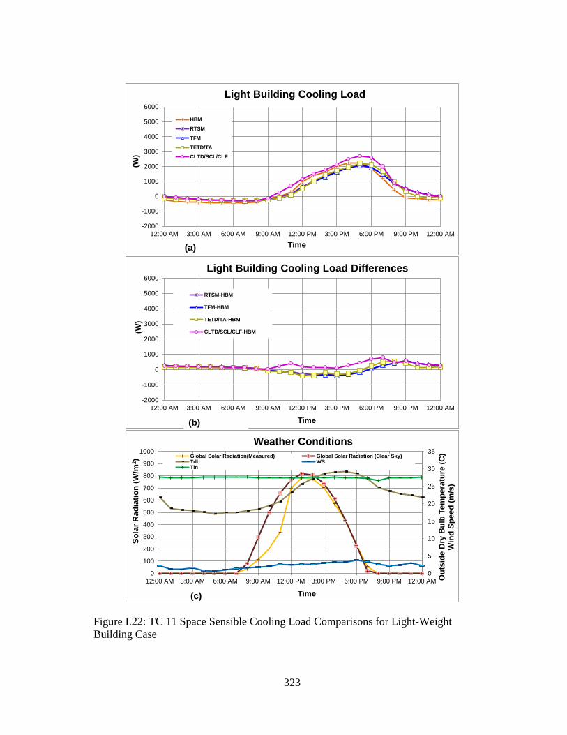
323
-2000
-1000
0
1000
2000
3000
4000
5000
6000
12:00 AM 3:00 AM 6:00 AM 9:00 AM 12:00 PM 3:00 PM 6:00 PM 9:00 PM 12:00 AM
(W)
Time
Light Building Cooling Load
HBM
RTSM
TFM
TETD/TA
CLTD/SCL/CLF
(a)
-2000
-1000
0
1000
2000
3000
4000
5000
6000
12:00 AM 3:00 AM 6:00 AM 9:00 AM 12:00 PM 3:00 PM 6:00 PM 9:00 PM 12:00 AM
(W)
Time
Light Building Cooling Load Differences
RTSM-HBM
TFM-HBM
TETD/TA-HBM
CLTD/SCL/CLF-HBM
(b)(b)(b)(b)(b)
0
5
10
15
20
25
30
35
0
100
200
300
400
500
600
700
800
900
1000
12:00 AM 3:00 AM 6:00 AM 9:00 AM 12:00 PM 3:00 PM 6:00 PM 9:00 PM 12:00 AM Ou
tsid
e D
ry B
ulb
Te
mp
era
ture
(C
)W
ind
Sp
ee
d (
m/s
)
So
lar
Ra
dia
tio
n (
W/m
2)
Time
Weather Conditions
Global Solar Radiation(Measured) Global Solar Radiation (Clear Sky)Tdb WSTin
(c)
Figure I.22: TC 11 Space Sensible Cooling Load Comparisons for Light-Weight
Building Case

324
-2000
-1000
0
1000
2000
3000
4000
5000
6000
12:00 AM 3:00 AM 6:00 AM 9:00 AM 12:00 PM 3:00 PM 6:00 PM 9:00 PM 12:00 AM
(W)
Time
Heavy Building Cooling Load
HBM
RTSM
TFM
TETD/TA
CLTD/SCL/CLF
-2000
-1000
0
1000
2000
3000
4000
5000
6000
12:00 AM 3:00 AM 6:00 AM 9:00 AM 12:00 PM 3:00 PM 6:00 PM 9:00 PM 12:00 AM
(W)
Time
Heavy Building Cooling Load Differences
RTSM-HBM
TFM-HBM
TETD/TA-HBM
CLTD/SCL/CLF-HBM
(b)(b)(b)(b)(b)
0
5
10
15
20
25
30
35
0
100
200
300
400
500
600
700
800
900
1000
12:00 AM 3:00 AM 6:00 AM 9:00 AM 12:00 PM 3:00 PM 6:00 PM 9:00 PM 12:00 AM Ou
tsid
e D
ry B
ulb
Te
mp
era
ture
(C
)W
ind
Sp
ee
d (
m/s
)
So
lar
Rad
iati
on
(W
/m2)
Time
Weather Conditions
Global Solar Radiation(Measured) Global Solar Radiation (Clear Sky)Tdb WSTin
(c)
(a)
Figure I.23: TC 12 Space Sensible Cooling Load Comparisons for Heavy-Weight
Building Case

325
-2000
-1000
0
1000
2000
3000
4000
5000
6000
12:00 AM 3:00 AM 6:00 AM 9:00 AM 12:00 PM 3:00 PM 6:00 PM 9:00 PM 12:00 AM
(W)
Time
Light Building Cooling Load
HBM
RTSM
TFM
TETD/TA
CLTD/SCL/CLF
(a)
-2000
-1000
0
1000
2000
3000
4000
5000
6000
12:00 AM 3:00 AM 6:00 AM 9:00 AM 12:00 PM 3:00 PM 6:00 PM 9:00 PM 12:00 AM
(W)
Time
Light Building Cooling Load Differences
RTSM-HBM
TFM-HBM
TETD/TA-HBM
CLTD/SCL/CLF-HBM
(b)(b)(b)(b)(b)
0
5
10
15
20
25
30
35
0
100
200
300
400
500
600
700
800
900
1000
12:00 AM 3:00 AM 6:00 AM 9:00 AM 12:00 PM 3:00 PM 6:00 PM 9:00 PM 12:00 AM Ou
tsid
e D
ry B
ulb
Te
mp
era
ture
(C
)W
ind
Sp
ee
d (
m/s
)
So
lar
Ra
dia
tio
n (
W/m
2)
Time
Weather Conditions
Global Solar Radiation(Measured) Global Solar Radiation (Clear Sky)Tdb WSTin
(c)
Figure I.24: TC 12 Space Sensible Cooling Load Comparisons for Light-Weight
Building Case
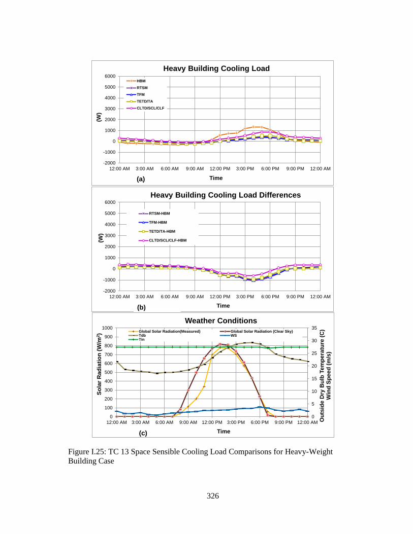
326
-2000
-1000
0
1000
2000
3000
4000
5000
6000
12:00 AM 3:00 AM 6:00 AM 9:00 AM 12:00 PM 3:00 PM 6:00 PM 9:00 PM 12:00 AM
(W)
Time
Heavy Building Cooling Load
HBM
RTSM
TFM
TETD/TA
CLTD/SCL/CLF
-2000
-1000
0
1000
2000
3000
4000
5000
6000
12:00 AM 3:00 AM 6:00 AM 9:00 AM 12:00 PM 3:00 PM 6:00 PM 9:00 PM 12:00 AM
(W)
Time
Heavy Building Cooling Load Differences
RTSM-HBM
TFM-HBM
TETD/TA-HBM
CLTD/SCL/CLF-HBM
(b)(b)(b)(b)(b)
0
5
10
15
20
25
30
35
0
100
200
300
400
500
600
700
800
900
1000
12:00 AM 3:00 AM 6:00 AM 9:00 AM 12:00 PM 3:00 PM 6:00 PM 9:00 PM 12:00 AM Ou
tsid
e D
ry B
ulb
Te
mp
era
ture
(C
)W
ind
Sp
ee
d (
m/s
)
So
lar
Rad
iati
on
(W
/m2)
Time
Weather Conditions
Global Solar Radiation(Measured) Global Solar Radiation (Clear Sky)Tdb WSTin
(c)
(a)
Figure I.25: TC 13 Space Sensible Cooling Load Comparisons for Heavy-Weight
Building Case

327
-2000
-1000
0
1000
2000
3000
4000
5000
6000
12:00 AM 3:00 AM 6:00 AM 9:00 AM 12:00 PM 3:00 PM 6:00 PM 9:00 PM 12:00 AM
(W)
Time
Light Building Cooling Load
HBM
RTSM
TFM
TETD/TA
CLTD/SCL/CLF
(a)
-2000
-1000
0
1000
2000
3000
4000
5000
6000
12:00 AM 3:00 AM 6:00 AM 9:00 AM 12:00 PM 3:00 PM 6:00 PM 9:00 PM 12:00 AM
(W)
Time
Light Building Cooling Load Differences
RTSM-HBM
TFM-HBM
TETD/TA-HBM
CLTD/SCL/CLF-HBM
(b)(b)(b)(b)(b)
0
5
10
15
20
25
30
35
0
100
200
300
400
500
600
700
800
900
1000
12:00 AM 3:00 AM 6:00 AM 9:00 AM 12:00 PM 3:00 PM 6:00 PM 9:00 PM 12:00 AM Ou
tsid
e D
ry B
ulb
Te
mp
era
ture
(C
)W
ind
Sp
ee
d (
m/s
)
So
lar
Ra
dia
tio
n (
W/m
2)
Time
Weather Conditions
Global Solar Radiation(Measured) Global Solar Radiation (Clear Sky)Tdb WSTin
(c)
Figure I.26: TC 13 Space Sensible Cooling Load Comparisons for Light-Weight
Building Case
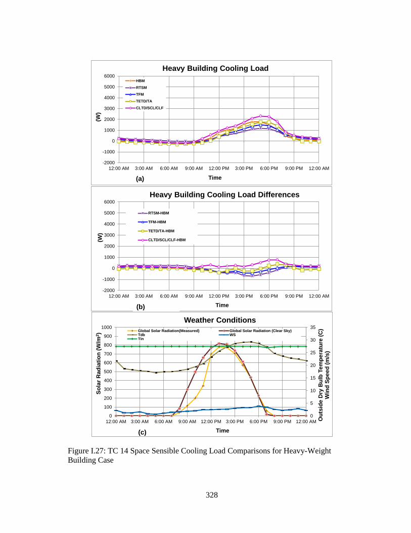
328
-2000
-1000
0
1000
2000
3000
4000
5000
6000
12:00 AM 3:00 AM 6:00 AM 9:00 AM 12:00 PM 3:00 PM 6:00 PM 9:00 PM 12:00 AM
(W)
Time
Heavy Building Cooling Load
HBM
RTSM
TFM
TETD/TA
CLTD/SCL/CLF
-2000
-1000
0
1000
2000
3000
4000
5000
6000
12:00 AM 3:00 AM 6:00 AM 9:00 AM 12:00 PM 3:00 PM 6:00 PM 9:00 PM 12:00 AM
(W)
Time
Heavy Building Cooling Load Differences
RTSM-HBM
TFM-HBM
TETD/TA-HBM
CLTD/SCL/CLF-HBM
(b)(b)(b)(b)(b)
0
5
10
15
20
25
30
35
0
100
200
300
400
500
600
700
800
900
1000
12:00 AM 3:00 AM 6:00 AM 9:00 AM 12:00 PM 3:00 PM 6:00 PM 9:00 PM 12:00 AM Ou
tsid
e D
ry B
ulb
Te
mp
era
ture
(C
)W
ind
Sp
ee
d (
m/s
)
So
lar
Rad
iati
on
(W
/m2)
Time
Weather Conditions
Global Solar Radiation(Measured) Global Solar Radiation (Clear Sky)Tdb WSTin
(c)
(a)
Figure I.27: TC 14 Space Sensible Cooling Load Comparisons for Heavy-Weight
Building Case
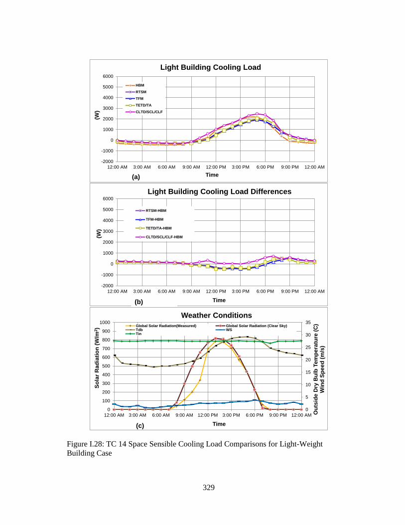
329
-2000
-1000
0
1000
2000
3000
4000
5000
6000
12:00 AM 3:00 AM 6:00 AM 9:00 AM 12:00 PM 3:00 PM 6:00 PM 9:00 PM 12:00 AM
(W)
Time
Light Building Cooling Load
HBM
RTSM
TFM
TETD/TA
CLTD/SCL/CLF
(a)
-2000
-1000
0
1000
2000
3000
4000
5000
6000
12:00 AM 3:00 AM 6:00 AM 9:00 AM 12:00 PM 3:00 PM 6:00 PM 9:00 PM 12:00 AM
(W)
Time
Light Building Cooling Load Differences
RTSM-HBM
TFM-HBM
TETD/TA-HBM
CLTD/SCL/CLF-HBM
(b)(b)(b)(b)(b)
0
5
10
15
20
25
30
35
0
100
200
300
400
500
600
700
800
900
1000
12:00 AM 3:00 AM 6:00 AM 9:00 AM 12:00 PM 3:00 PM 6:00 PM 9:00 PM 12:00 AM Ou
tsid
e D
ry B
ulb
Te
mp
era
ture
(C
)W
ind
Sp
ee
d (
m/s
)
So
lar
Ra
dia
tio
n (
W/m
2)
Time
Weather Conditions
Global Solar Radiation(Measured) Global Solar Radiation (Clear Sky)Tdb WSTin
(c)
Figure I.28: TC 14 Space Sensible Cooling Load Comparisons for Light-Weight
Building Case
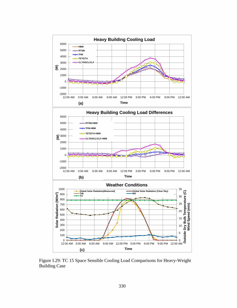
330
-2000
-1000
0
1000
2000
3000
4000
5000
6000
12:00 AM 3:00 AM 6:00 AM 9:00 AM 12:00 PM 3:00 PM 6:00 PM 9:00 PM 12:00 AM
(W)
Time
Heavy Building Cooling Load
HBM
RTSM
TFM
TETD/TA
CLTD/SCL/CLF
-2000
-1000
0
1000
2000
3000
4000
5000
6000
12:00 AM 3:00 AM 6:00 AM 9:00 AM 12:00 PM 3:00 PM 6:00 PM 9:00 PM 12:00 AM
(W)
Time
Heavy Building Cooling Load Differences
RTSM-HBM
TFM-HBM
TETD/TA-HBM
CLTD/SCL/CLF-HBM
(b)(b)(b)(b)(b)
0
5
10
15
20
25
30
35
0
100
200
300
400
500
600
700
800
900
1000
12:00 AM 3:00 AM 6:00 AM 9:00 AM 12:00 PM 3:00 PM 6:00 PM 9:00 PM 12:00 AM Ou
tsid
e D
ry B
ulb
Te
mp
era
ture
(C
)W
ind
Sp
ee
d (
m/s
)
So
lar
Rad
iati
on
(W
/m2)
Time
Weather Conditions
Global Solar Radiation(Measured) Global Solar Radiation (Clear Sky)Tdb WSTin
(c)
(a)
Figure I.29: TC 15 Space Sensible Cooling Load Comparisons for Heavy-Weight
Building Case
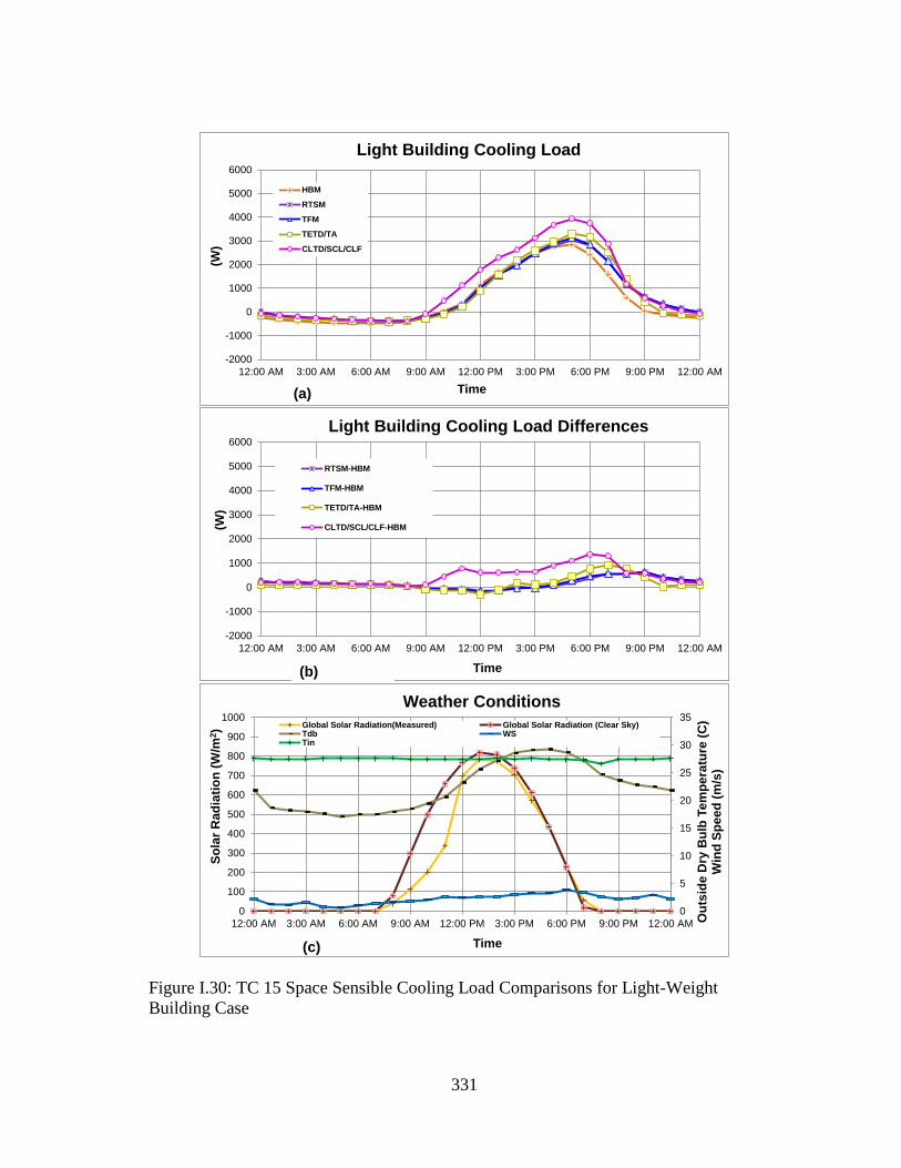
331
-2000
-1000
0
1000
2000
3000
4000
5000
6000
12:00 AM 3:00 AM 6:00 AM 9:00 AM 12:00 PM 3:00 PM 6:00 PM 9:00 PM 12:00 AM
(W)
Time
Light Building Cooling Load
HBM
RTSM
TFM
TETD/TA
CLTD/SCL/CLF
(a)
-2000
-1000
0
1000
2000
3000
4000
5000
6000
12:00 AM 3:00 AM 6:00 AM 9:00 AM 12:00 PM 3:00 PM 6:00 PM 9:00 PM 12:00 AM
(W)
Time
Light Building Cooling Load Differences
RTSM-HBM
TFM-HBM
TETD/TA-HBM
CLTD/SCL/CLF-HBM
(b)(b)(b)(b)(b)
0
5
10
15
20
25
30
35
0
100
200
300
400
500
600
700
800
900
1000
12:00 AM 3:00 AM 6:00 AM 9:00 AM 12:00 PM 3:00 PM 6:00 PM 9:00 PM 12:00 AM Ou
tsid
e D
ry B
ulb
Te
mp
era
ture
(C
)W
ind
Sp
ee
d (
m/s
)
So
lar
Ra
dia
tio
n (
W/m
2)
Time
Weather Conditions
Global Solar Radiation(Measured) Global Solar Radiation (Clear Sky)Tdb WSTin
(c)
Figure I.30: TC 15 Space Sensible Cooling Load Comparisons for Light-Weight
Building Case