Embed Size (px)
Citation preview
Department of Water Resources
Analysis of Archived Samples to Assess Patterns of Historic Invasive Bivalve Biomass A Report to the Delta Science Council
Karen Gehrts, Dan Riordan, Rachel August, and Analisa Canepa 12/1/2011

2
3
Table of Contents Introduction .................................................................................................................................................. 5
Methods ....................................................................................................................................................... 6
Sampling .............................................................................................................................................. 6
Resorting ............................................................................................................................................. 6
Image Analysis ................................................................................................................................... 6
QA/QC of Image Analysis Data........................................................................................................ 6
IA Raw Data ........................................................................................................................................ 7
Live Sort Data ..................................................................................................................................... 7
Results and Discussion ............................................................................................................................. 7
Defining recruits and adults .............................................................................................................. 7
Site D28A............................................................................................................................................. 7
Site D4 ................................................................................................................................................. 8
Future Directions ........................................................................................................................................ 8
Literature Cited ........................................................................................................................................... 9
Figures 1-12 .............................................................................................................................................. 11
Appendix A ................................................................................................................................................ 24
Standard Operating Procedure for Imagine Analysis ................................................................. 24

4
5
Introduction Invasive bivalves are considered to be a major sink of primary productivity in the upper San Francisco estuary (estuary). Alpine and Cloern (1992), showed that seasonal phytoplankton blooms disappeared after the invasive bivalve Corbula amurensis invaded the estuary. Lucas et al. (2002), found that Sacramento-San Joaquin Delta habitats where the invasive bivalve Corbicula fluminea were abundant were net sinks to phytoplankton biomass. Lopez et al. (2006), concurred with findings that while shallow water habitats in the estuary could have high phytoplankton productivity, those heavily colonized by C. fluminea are net sinks of phytoplankton biomass. The work of Lucas et al. (2002) and Lopez et al. (2006) support the concept that bivalve grazing is an important factor in determining overall ecosystem function in the estuary. Thus, investigations of invasive bivalve population dynamics and grazing pressure over temporal and spatial gradients are important when considering restoration plans for the system. The recognized declines in several delta fish populations have heightened interest in the pelagic food web of the estuary. Several populations of fish that prey on zooplankton are in decline (http://www.calwater.ca.gov/DeltaFishPopulations/Enclosure_1.pdf), with delta smelt in particular, showing signs of starvation (Bennett 2005). Jassby et al. (2002) report that overall primary production in the estuary is low (70g C m-2) and indicate that primary production lost to invasive bivalve grazing is a key factor in limiting net productivity in the system. Several populations of primary consumers (zooplankton) have declined in recent decades, concurrent with the introduction of the invasive bivalve C. amurensis, and appear to be food limited (Kimmerer and Orsi 1996, Orsi and Mecum 1996, Mueller-Solger et al 2002). Benthic bivalves are both ubiquitous and abundant in the estuary (Carlton et al. 1990, Hymanson 1991, Hymanson et al.1994). These bivalves are also dominant in macrobenthic assemblages (Hymanson et al.1994). Accurate estimates of bivalve biomass are necessary for assessments of carbon transfer and also contaminants among the food webs. Invasive bivalve species have been found to assimilate trace contaminants (Brown and Luoma 1995, Luoma and Linville 1995) and are known to transfer them among trophic levels within the food web (Stewart et al. 2004). Investigations of historic patterns of invasive bivalve population biomass from long-term records will yield information about the relationships between bivalve populations, including benthic grazing pressure and environmental factors, such as hydrologic year type and water management practices. Fortunately, a legacy of environmental monitoring by the Interagency Ecological Program (IEP) Environmental Monitoring Program (EMP) has accumulated a wealth of high-quality, archived benthic invertebrate samples with which we may investigate historic bivalve populations. Analysis of patterns of bivalve biomass both over time through a range of hydrologic conditions, can be conducted on archived historic samples. The purpose of this study was to estimate the biomass (g C m-2) of invasive
6
bivalve species from preserved samples. This study addresses changes in invasive bivalve populations over time by analyzing archived samples from monthly or near-monthly monitoring, conducted over a 30 year time period, in the lower Sacramento River near Collinsville (site D4-L) and in the lower San Joaquin River system in Old River (site D28A-L).
Methods
Sampling The research vessels San Carlos, Endeavor, and Whaler, each equipped with either a hydraulic winch or davit, and a Ponar dredge were used to conduct sampling. The Ponar dredge samples a bottom area of 0.053 m2. The contents of the dredge were washed over a Standard No. 30 stainless steel mesh screen (0.595 mm openings) to remove as much substrate as possible. All material remaining on the screen was preserved in approximately 20% buffered formaldehyde containing rose bengal dye and was transported to the laboratory for analysis. The benthic macroinvertebrate sampling methodology used in this program is described in Standard Methods (APHA, 1998). In the laboratory, the field preservative was decanted and the sample was washed with deionized water over a Standard No. 30 stainless steel mesh screen. Organisms were then placed in 70% ethyl alcohol for preservation. Hydrozoology (P.O. Box 682, Newcastle, CA 95658), a private laboratory under contract with DWR, identified and enumerated organisms in the macrofaunal samples.
Resorting One sample from each station per month from January, 1981 to September, 2006 was selected at random for analysis. Up until 2003, Hydrozoology staff processed each sample and recombined all organisms into a single jar. This made it necessary to re-sort each randomly picked monthly sample by species. This was accomplished using a stereoscopic dissecting microscope.
Image Analysis Clams were removed from their vials, dried on a 106 µm sieve, and placed on a tray for imaging. Once on the tray, a picture was taken of with a Sony XCD-X710CR camera. Each image was captured and the maximum shell length of every clam, in millimeters, was determined using HLImage++ 2005 software. (See Standard Operating Procedure in Appendix A). Data was then transferred to a Microsoft Excel spreadsheet where it was later used to make abundance and biomass determinations.
QA/QC of Image Analysis Data After pictures were taken, the maximum shell length of one clam was measured with digital calipers. This value was used to verify that the image analysis (IA) software was calibrated correctly and returning accurate measurements. If the value recorded by the
7
software was greater than one millimeter different than what was measured with the calipers, the camera was re-calibrated and another picture was taken. Each picture was also reviewed to ensure that all clams for which values were recorded were in fact clams (i.e. not a bit of dust, a shell fragment, an odd reflection of light, etc.). If foreign objects were detected, another picture of the cluster was taken and the visual inspection repeated.
IA Raw Data All IA data was transferred from their original spreadsheets and combined (according to species and site) into another spreadsheet where abundance and biomass data could be calculated. Data was then placed into pivot tables and graphed accordingly.
Live Sort Data Beginning in July, 2006, an extra sample was collected at each site. These samples were processed in the field as previously stated. However, instead of being preserved in formalin, they were stored in water from their respective sites and refrigerated. They were then transported to the lab where all live C. fluminea and C. amurensis were removed. Next, the clams were separated and grouped according to species and size (0-0.99 mm, 1.00-1.99, etc.) and then dried at 100oC for two weeks. Once dry, a dry weight (DW) was obtained and they were then ashed at 500oC. Ash-free dry weights (AFDW) were obtained and the differences between those and DW were used to determine biomass per square meter. Shell length and biomass data from these clams were then used to generate regression equations for converting size class of preserved clams to biomass. That equation is as follows: Biomass m-2 = (m * ln[size class] + b)(# of individuals * 19)
Results and Discussion
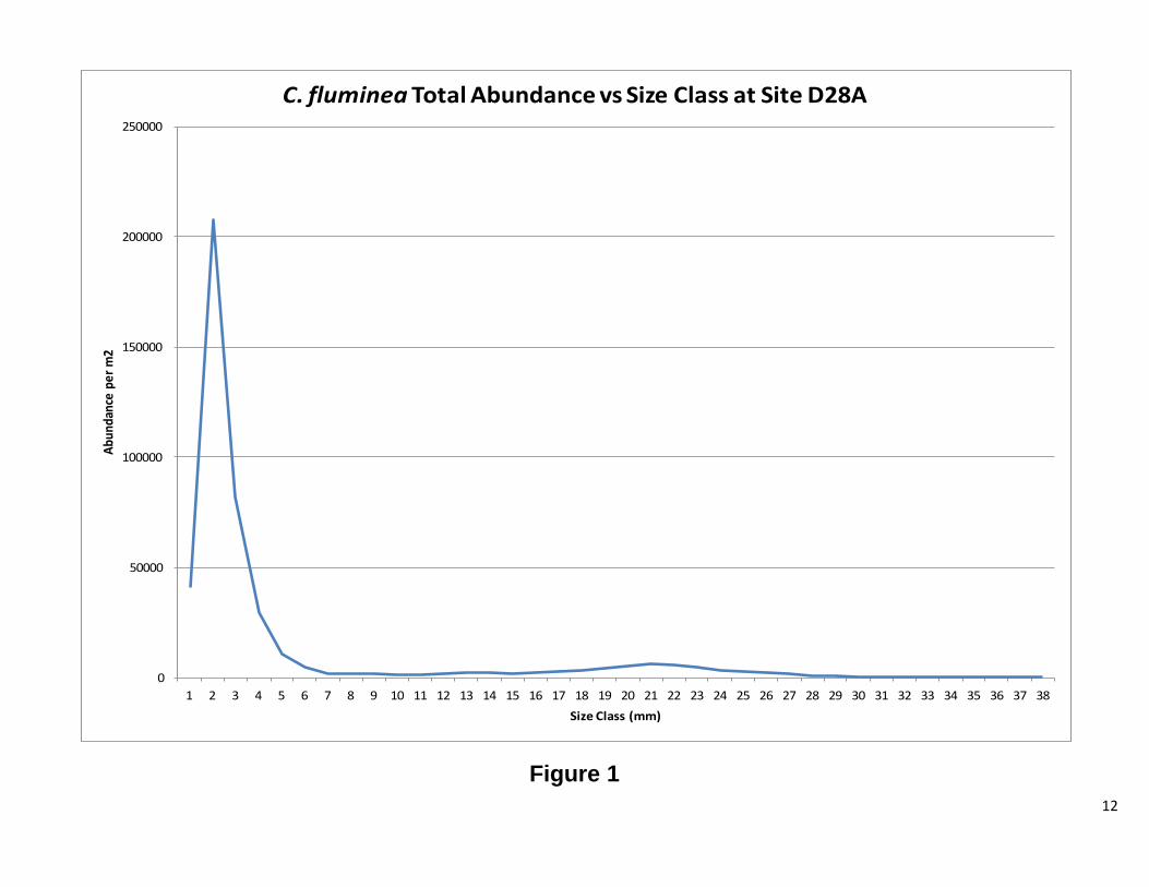
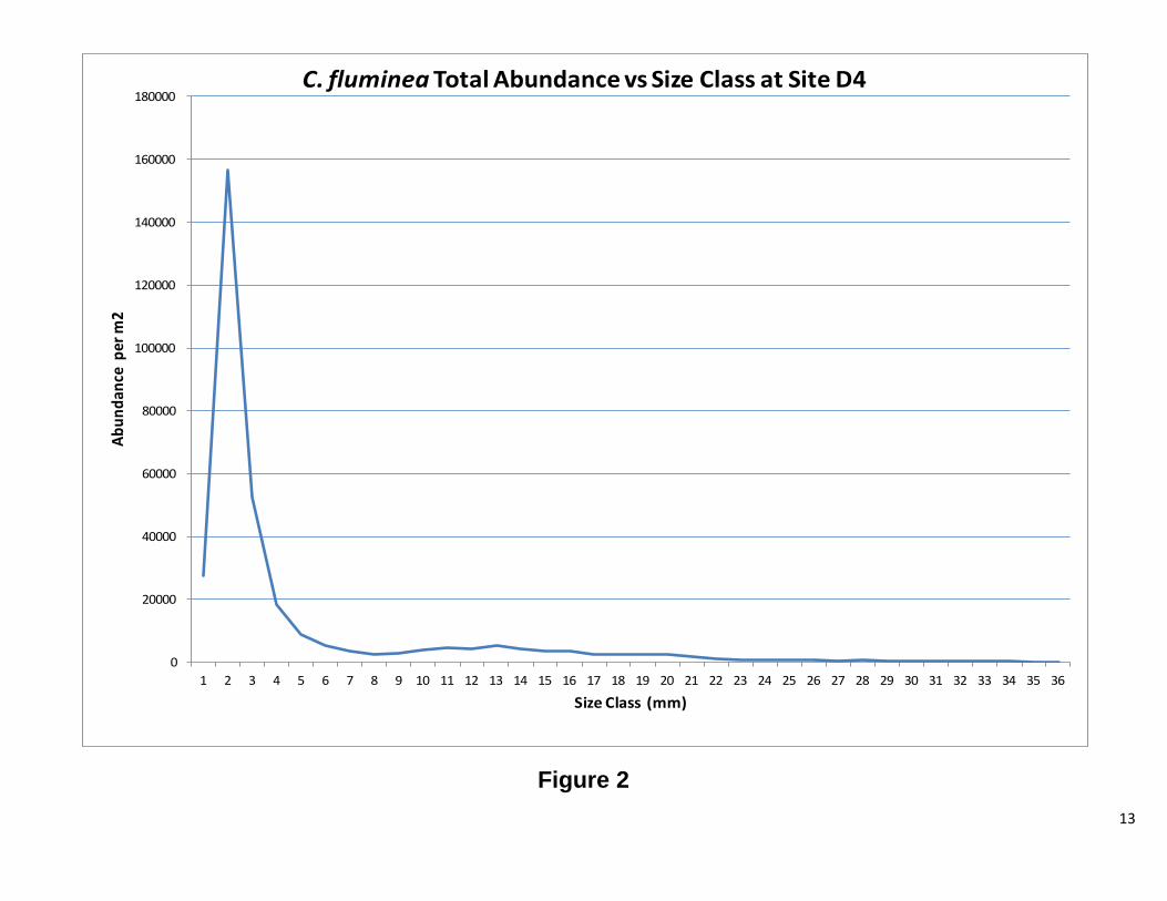
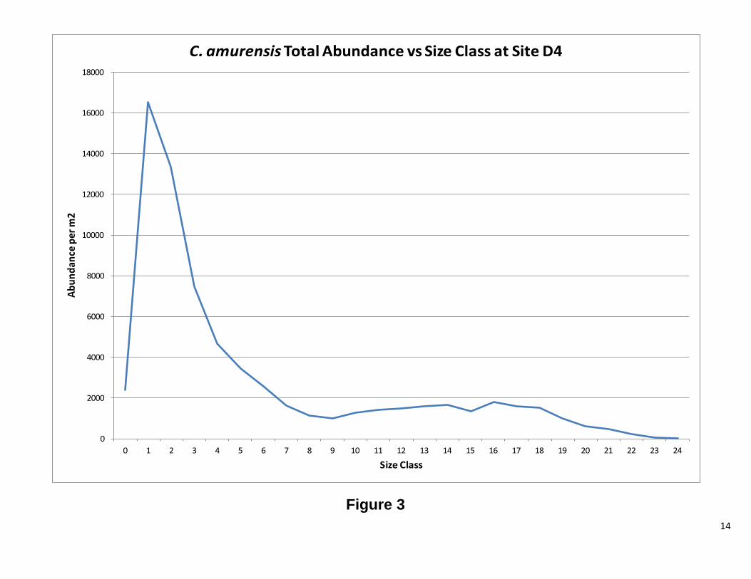
Defining recruits and adults We were unable to model the age structure of our population for this report; however, for R reproducing populations, organisms produce a larger number of offspring. The majority of these offspring do not reach adulthood (Vandermeer, JH, Goldberg, DE, 2003) It is therefore reasonable to suggest that one can determine the approximate size at which the population reaches adulthood and begins reproducing. After analyzing Figures 1 and 2, it was determined that an adult C. fluminea would be any clam greater than 6 mm in maximum shell length. Figure 3 was used to determine that an adult C. amurensis would be any clam greater than 8 mm in maximum shell length.
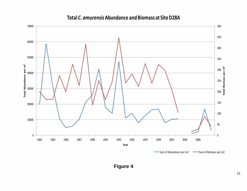
Site D28A Overall, abundance and biomass of C. fluminea at site D28A track each other closely (Figure 4). Population dynamics were normal, with more recruits than adults, except from 1984 to 1987 and again in 1994-2000. In both instances the biomass was much greater than the abundance.
8
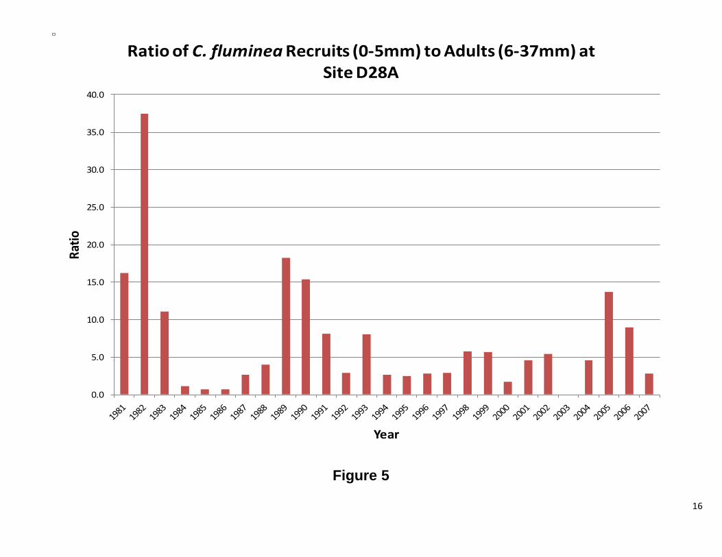
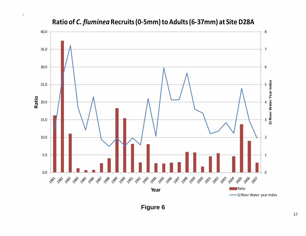
Figure 5 shows the ratio of recruits vs. adults over time, where the total number of recruits in a given year was divided by the total number of adults. A high value indicates significant recruitment. The variance over time will show if the population was stable and when recruitment events took place. The ratio of recruits to larger, reproducing, clams has varied greatly. In the early 1980’s, the population was dominated by small clams. The mid 1980’s saw a shift towards an adult dominated population (Figure 5). Recruitment during this time was also very low. This pattern repeated itself in the mid 1990’s and in 2000, but to a lesser extent. When the ratio was plotted against water year (Figure 6), no clear patterns were observed.
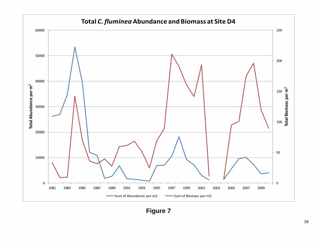
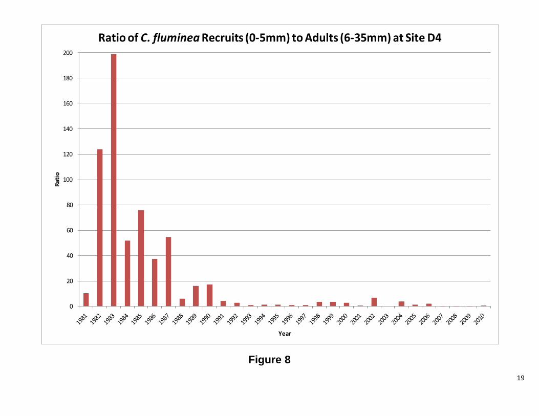
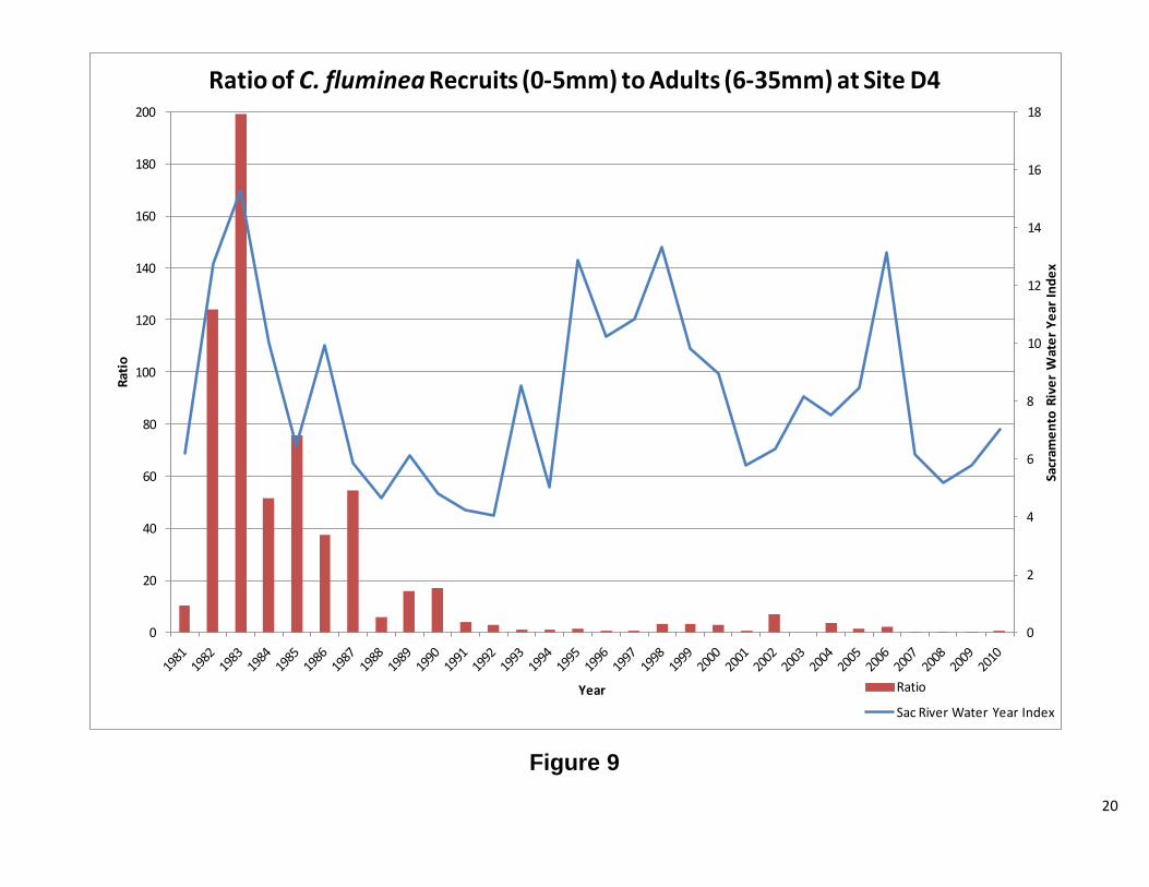
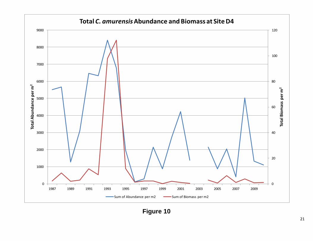
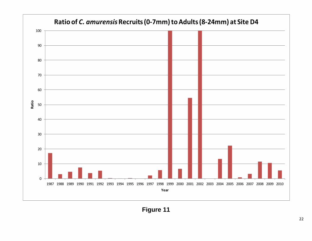
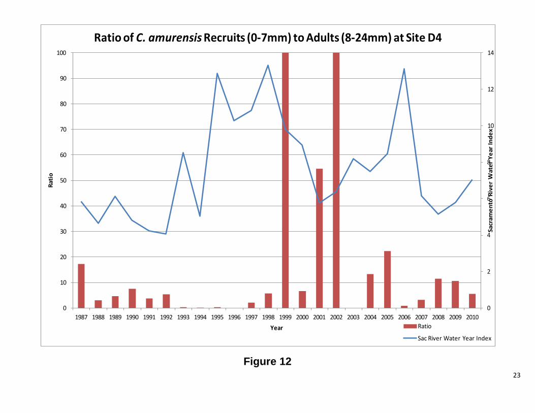
Site D4 This station has both C. fluminea and C. amurensis. The results for each clam will be discussed separelty. Overall, abundance and biomass for C. fluminea tracked each other. There were periods of significant difference between the two, but the overall pattern is the same. Figure 7 shows high abundance for C. fluminea prior to 1987. After 1987, biomass increased while abundance significantly decreased. The graph of the ratio of recruits to adults (Figure 8) shows that the cause of the high abundance was a population dominated by smaller clams. After 1987, the ratio dropped considerably, indicating fewer recruits and more adults. When the ratio is plotted against water year, there appears to be a correlation between the two, until 1987, when no clear patterns were observed (Figure 8). Interestingly, the change in population structure coincides with the introduction of C. amurensis to the system (Cohen and Carlton, 1995). As with C. fluminea abundance and biomass, for C. amurensis, tracked each other. The abundance has varied greatly over the years, while the biomass, with the remarkable exception of 1993 and 1994, has remained relatively stable. At the beginning of the C amurensis invasion, the population consisted of a large proportion of smaller clams. During the early 1990’s, the population shifted to mostly adults. During 1999 and 2000, the population was exclusively recruits with 2001, 2004, and 2005 also heavily dominated by smaller clams. The ratio appears to be following the water year index; however, further analysis is needed. There was a low water year index, while the population was establishing itself, and as the index rose, so did the adult population. As the water year index dropped the population consisted of mostly recruits (Figure 12 1987-2002). This pattern repeats itself from 2004 to 2010, but to a lesser extent. Future Directions
This project has allowed for a cursory look at invasive bivalve populations at two locations in the estuary. Though this study was informative as to how population and biomass have changed over time, the reasons behind these trends are still unknown. Fortunately, in addition to archived benthic samples, the EMP has accumulated a wealth of water quality, phytoplankton, and zooplankton data dating back to 1975. The
9
natural progression of this study would be to analyze trends in the bivalve community against those observed in the water quality data. This, hopefully, would lead to a more clear understanding as to why changes in bivalve populations occur and what their role is at an ecosystem level.
Literature Cited Alpine, AE, Cloern, JE (1992) Trophic interactions and direct physical effects control
phytoplankton biomass and production in an estuary. Limnol Oceanogr 37:946-955
[APHA] American Public Health Association, American Water Works Association, and
Water Environmental Federation. (1998). Standard Methods for the Examination of Water and Wastewater [Standard Methods] (20th ed.). Washington DC, 10.60-10.74.
Bennett, WA (2005) Critical Assessment of the Delta Smelt Population in the San
Francisco Estuary, California. San Francisco Estuary and Watershed Science. 3 (2).
Brown, CL, Luoma, SN (1995) Use of the euryhaline bivalve Potamocorbula amurensis
as a biosentinel species to assess trace metal contamination in San Francisco Bay. Marine Ecology Progress Series 124:129-142.
Carlton, JT, Thompson, JK, Schemel, LE, Nichols, FH (1990) Remarkable invasion of
San Francisco Bay (California, USA) by the Asian clam Potamocorbula amurensis. I. Introduction and dispersal. Marine Ecology Progress Series 66:81-94.
Cohen, AN, Carlton, JT (1995) Nonindigenous Aquatic Species in a United States
Estuary: A case study of the biological invasions of the San Francisco Bay and Delta. Report No. Report No. PB96-166525, United States Fish and Wildlife Service, Washington D. C.
Hymanson, Z (1991) Results of a Spatially Intensive Survey for Potamocorbula
amurensis in the upper San Francisco Bay Estuary. Report No. 30, Interagency Ecological Studies Program for the Sacramento-San Joaquin Estuary, Sacramento, CA.
Hymanson, Z, Mayer, D, Steinbeck, J (1994) Long-term trends in benthos abundance
and persistence in the upper Sacramento-San Joaquin Estuary: Summary report 1980-1990. Report No. 38, Interagency Ecological Program for the San Francisco Bay/Delta Estuary.
10
Jassby, AD, Cloern, JE, Cole, BE (2002) Annual primary production: Patterns and mechanisms of change in a nutrient-rich tidal ecosystem. Limnol Oceanogr 47:698-712.
Kimmerer, WJ, Orsi, JJ (1996) Changes in the zooplankton of the San Francisco Bay
Estuary since the introduction of the clam Potamocorbula amurensis. In: Hollibaugh JT (ed) San Francisco Bay the ecosystem. Pacific Division of the American Association for the Advancement of Science, San Francisco, p 542pp.
Lopez, CB, Cloern, JE, Schraga, TS, Little, AJ, Lucas, LV, Thompson, JK, Burau, JR
(2006) Ecological Values of Shallow-Water Habitats: Implications for the Restoration of Disturbed Ecosystems. Ecosystems 9:422-440.
Lucas, LV, Cloern, JE, Thompson, JK, Monsen, NE (2002) Functional variability of
habitats within the Sacramento-San Joaquin Delta: restoration implications. Ecological Applications 12:1528-1547.
Luoma, SN, Linville, R (1995) A Comparison of Selenium and Mercury Concentrations
in Transplanted and Resident Bivalves from North San Francisco Bay. Regional Monitoring Program for Trace Substances, 1995 Annual Report, SFEI Publications 160-170.
Muller-Solger, A., Jassby, A., and Muller-Navarra, D., 2002. Nutritional Quality of Food
Resources for Zooplankton (Daphina) in a Tidal Freshwater System (Sacramento-San Joaquin River Delta). Limnol. Oceanogr., 47 (5): 1468-1476.
Orsi, JJ, Mecum, WL (1996) Food Limitation as the Probable Cause of a Long-term
Decline in the Abundance of Neomysis mercedes the Opossum Shrimp in the Sacramento-San Joaquin Estuary. In: Hollibaugh JT (ed). AAAS, p 375-401.
Stewart, AR, Luoma, SN, Schlekat, CE, MDoblin, MA, Hieb, K (2004) Food Web
Pathway Determines How Selenium Affect Aquatic Ecosystems: A San Francisco Bay Case Study. Environmental Science and technology 38:4519-4526 .
Vandermeer, JH, Goldberg, DE (2003) Population Ecology, First Principles. Princeton:
Princeton University Press.
11
Figures 1-12
12
Figure 1
0
50000
100000
150000
200000
250000
1 2 3 4 5 6 7 8 9 10 11 12 13 14 15 16 17 18 19 20 21 22 23 24 25 26 27 28 29 30 31 32 33 34 35 36 37 38
Abun
danc
e pe
r m2
Size Class (mm)
C. fluminea Total Abundance vs Size Class at Site D28A
13
Figure 2
0
20000
40000
60000
80000
100000
120000
140000
160000
180000
1 2 3 4 5 6 7 8 9 10 11 12 13 14 15 16 17 18 19 20 21 22 23 24 25 26 27 28 29 30 31 32 33 34 35 36
Abun
danc
e p
er m
2
Size Class (mm)
C. fluminea Total Abundance vs Size Class at Site D4
14
Figure 3
0
2000
4000
6000
8000
10000
12000
14000
16000
18000
0 1 2 3 4 5 6 7 8 9 10 11 12 13 14 15 16 17 18 19 20 21 22 23 24
Abun
danc
e pe
r m2
Size Class
C. amurensis Total Abundance vs Size Class at Site D4
15
Figure 4
0
50
100
150
200
250
300
350
400
450
500
0
10000
20000
30000
40000
50000
60000
70000
1981 1983 1985 1987 1989 1991 1993 1995 1997 1999 2001 2004 2006
Tota
l B
iom
ass
pe
r m
2
Tota
l A
bu
nd
ance
pe
r m
2
Year
Total C. amurensis Abundance and Biomass at Site D28A
Sum of Abundance per m2 Sum of Biomass per m2
16
Figure 5
0.0
5.0
10.0
15.0
20.0
25.0
30.0
35.0
40.0
Ratio
Year
Ratio of C. fluminea Recruits (0-5mm) to Adults (6-37mm) at Site D28A
17
Figure 6
0
1
2
3
4
5
6
7
8
0.0
5.0
10.0
15.0
20.0
25.0
30.0
35.0
40.0
SJ R
iver
Wat
er Y
ear
Inde
x
Ratio
Year
Ratio of C. fluminea Recruits (0-5mm) to Adults (6-37mm) at Site D28A
RatioSJ River Water year Index
18
Figure 7
0
50
100
150
200
250
0
10000
20000
30000
40000
50000
60000
1981 1983 1985 1987 1989 1991 1993 1995 1997 1999 2001 2003 2005 2007 2009
Tota
l Bio
mas
s pe
r m2
Tota
l Abu
ndan
ce p
er m
2
Total C. fluminea Abundance and Biomass at Site D4
Sum of Abundance per m2 Sum of Biomass per m2
19
Figure 8
0
20
40
60
80
100
120
140
160
180
200Ra
tio
Year
Ratio of C. fluminea Recruits (0-5mm) to Adults (6-35mm) at Site D4
20
Figure 9
0
2
4
6
8
10
12
14
16
18
0
20
40
60
80
100
120
140
160
180
200
Sacr
amen
to R
iver
Wat
er Y
ear I
ndex
Ratio
Year
Ratio of C. fluminea Recruits (0-5mm) to Adults (6-35mm) at Site D4
Ratio
Sac River Water Year Index
21
Figure 10
0
20
40
60
80
100
120
0
1000
2000
3000
4000
5000
6000
7000
8000
9000
1987 1989 1991 1993 1995 1997 1999 2001 2003 2005 2007 2009
Tota
l Bio
mas
s pe
r m2
Tota
l Abu
ndan
ce p
er m
2
Total C. amurensis Abundance and Biomass at Site D4
Sum of Abundance per m2 Sum of Biomass per m2
22
Figure 11
0
10
20
30
40
50
60
70
80
90
100
1987 1988 1989 1990 1991 1992 1993 1994 1995 1996 1997 1998 1999 2000 2001 2002 2003 2004 2005 2006 2007 2008 2009 2010
Ratio
Year
Ratio of C. amurensis Recruits (0-7mm) to Adults (8-24mm) at Site D4
23
Figure 12
0
2
4
6
8
10
12
14
0
10
20
30
40
50
60
70
80
90
100
1987 1988 1989 1990 1991 1992 1993 1994 1995 1996 1997 1998 1999 2000 2001 2002 2003 2004 2005 2006 2007 2008 2009 2010
Sacr
amen
to R
iver
Wat
er Y
ear I
ndex
Ratio
Year
Ratio of C. amurensis Recruits (0-7mm) to Adults (8-24mm) at Site D4
Ratio
Sac River Water Year Index
24
Appendix A Standard Operating Procedure for Imagine Analysis
Method for Image Analysis:
Supplies:
Computer with HLI++ Samples
Chemical hood 3 in. diameter std.36 sieve
Paper Towels Spatula
Recycled Ethanol Bottle Ethanol (70%) wash bottle
Plastic graduated container Photography tray
Calibration card Calipers
Camera attached to stand
Procedure:
1. Turn on hood. Meanwhile, place the sieve over the plastic graduated container. Pour the clams out of their container into the sieve so that the graduated container collects the ethanol and the clams remain in the sieve.
2. Dry the clams using a paper towel to absorb the ethanol from the underside of the sieve (not touching the clams). Leaving moisture on the clams may cause glare in photos, resulting in bad measurements. Larger clams may be easier to dry by directly using a paper towel. Use compressed air (if available) to dry the smaller clams. If air is not available, lightly tap the side of the sieve to jar clams loose from the sieve. Use care when working with the air and tapping of the sieve to prevent clams from falling out of the sieve. Leaving them in the hood to dry ahead of time is also useful. It may be beneficial to have a separate person prep clams for photos and another working the actual camera.
3. It is best to choose a photography tray that is as flat as possible. Wipe off any debris that may be on the tray. Set clams larger than 10mm aside to measure with calipers. Clams that are too dark may also be measured more easily with calipers or the micrometer. Dump remaining clams from within the sieve into the photography tray. Using the spatula, arrange the smaller clams in groups, close together, without touching near the edge of the photography tray. It can be helpful to place clams in rows of even number to allow for easy count. Clams that are too close to each other may also affect measuring. Be careful, clams may be brittle and easy to break due to drying.
4. Double-Click the HLImage++ icon on the desktop.
25
5. Click on the camera icon on the very bottom right in the “Tools” palette. When you place your cursor over this icon it will read DCAM. Note: If Tools palette is missing click on “Tools” at the top of the screen and click “Show Toolbox”.
6. Load DCAM settings by clicking on “File” and click on “Open Settings.” The template is saved as C:\HLImage\Tools\HL_DCAM\IA Settings.dts. After “IA Settings.dts” is highlighted click the Open icon. If this file is missing go to step 7, otherwise continue to step 12.
Camera Set Up 7. The “Camera” box should read “SONY:WCD-X710CR v2.01A” 8. In the “Camera Format” box, choose “1024_x__768_Y__(Mono8)” from the drop
down menu. 9. In the “Frame Rate” box, choose “30” from the drop down menu. 10. In the “Raw Color Format” box, choose “GBRG” from the drop down menu. 11. Save settings as IA Settings.dts for preset configuration next time. 12. Click on the live box in the lower left corner of the “DCAM Picture Tool” palette and
expand the live window to a reasonable size. 13. Set the photography tray with the clams under the camera and bring it into focus in
the live window. Enlarge this window for better viewing. To adjust the focus, you may slide the camera up and down the photography stand by pressing down on the handle. You may also adjust the zoom on the camera itself. This is a tall ring around the camera just above the lens. You may also choose to adjust the aperture which is the ridged ring on top of the camera. (There is also another zoom just underneath the aperture ring.)
14. Only load calibrations when you are absolutely confident that the camera focus and zooms have not been touched since the last time you calibrated. CHANGING THE FOCUS AND ANY OF THE ZOOMS ON THE CAMERA WILL REQUIRE YOU TO RECALIBRATE. The aperture does not affect calibration. If the camera has moved or you are not confident that it has absolutely stayed the same, go to step 15. If you decide to load the calibration, open the calibration tool and select the calibration you wish to use. Make sure it is set on millimeters. Skip to step 20.
Calibration 15. Once clams are in focus, bring the calibration card into view. Just place any
calibration card in the tray, but away from the clams. DO NOT ADJUST FOCUS. You want to keep it focused for your clams. Try to keep the card as straight as possible.
16. Click the “Take Picture” button on the “DCAM Picture Tool” palette. Move the live picture out of the way, unclick the live checkbox, or minimize the DCAM picture tool to get rid of the live picture.
17. The picture that was just taken should be open in the program. Click on the “Calibration Tool” in the upper right corner of the “Tools” palette. The icon looks like a set of calipers.
18. Click on Point 1 in the calibration palette. Then click on the picture where you want point 1 to be. This should be the lower left corner tip of the calibration card. You want this to be as accurate as possible. It may help to zoom in for more accuracy
26
(increase the number on the drop down menu right under the file menu). Right clicking on the calibration point will turn the crosshair red, which allows you to precisely move the crosshair using the arrow keys. To remove and replace a point uncheck and recheck the point box to be changed. Repeat this procedure for points 2, 3, and 4, working clockwise around the calibration card. Afterwards, fill in the values under “World Coordinates (x,y)” according to what is written on the calibration card.
19. Click “Create” on the “Calibration” palette. In the box next to “Set” in the palette, use the drop down menu to choose millimeters and click “Set”. Return the zoom of the picture to 1. It may be worthwhile to save your calibration with the date as the name. Only load calibrations when you are absolutely confident that the camera focus and zooms have not been touched since the last time you calibrated. CHANGING THE FOCUS AND ANY OF THE ZOOMS ON THE CAMERA WILL REQUIRE YOU TO RECALIBRATE. The aperture does not affect calibration.
20. IMPORTANT: click “Attach to Image” on the calibration tool palette. 21. Click on the “Blob Analysis Tool” in the upper middle left on the tools palette. This
icon looks like different colored mis-shaped circles. If the program keeps skipping back to a previous picture, be sure that the manual thresholding box is unchecked. If this box remains checked for some reason, the program will keep reverting to an old picture.
22. Under the “File” menu click on “Open Settings” and open the file named “IA Settings.blb”. If the file is missing you must manually configure the blob analysis under the “Options” menu, by clicking on “Parameter Options”. Click “Delete ALL”. Click on “Major Axis” and then click “Add to List”. Alternately, you can just double click “Major Axis”. Click OK. It may be helpful to save these settings if they are not already saved.
23. On the “Blob Analysis” palette click the “Manual Thresholding” box. Move the “Minimum” bar left or right using the mouse or arrow keys. Move the bar until the clams in the picture are completely filled in pink. You may want to zoom in to the picture. This way you will be able to more accurately tell if the clams are completely filled in. If things are not filling in well or are filling in where they shouldn’t, please check the troubleshooting section on the end of this document.
24. Click “Find Blobs” in the “Blob Analysis” palette. A green circle will develop around each clam. You may need to adjust the “Blob Finding Options” under the “Options” menu. If you are finding very small clams you should have the minimum size around 20. If you are finding large clams, you should adjust the minimum size to be somewhere around 100-200. Once you change this number click “Apply” button and the “OK” button. This function can be quite helpful when looking at larger clams (5-10mm). The program will not consider anything smaller than what you have set as the minimum. This means that a shadow or other artifact smaller than the minimum size will not show up as a blob. Remember that very large clams and very dark clams may be hard to measure using image analysis. Any clams that give you too much trouble may be set aside to be measured by calipers.
25. When all measurements are taken, arrow through the blobs detected by the software to make sure each blob is corresponding with an actual clam and not a piece of debris on the photography tray. Make sure that the measurements make sense. It’s
27
worthwhile to double check a clam with calipers to see if the calibration was accurate.
26. Click on the “Transfer” menu on the “Blob Analysis” palette and click on “Send Data To Excel”. Delete any measurements that are not of clams. Then copy and paste all of the data into the spreadsheet titled “MASTER-IA & Caliper Data.xls.”
27. All image analyzer data should be copied into the IA Data tab. All caliper data should be imputed into the Caliper Data tab using the WinWedge calipers. To use the WinWedge calipers, plug the calipers into the computer with the appropriate serial cable, have the Caliper-IA Settings.SW3 program (found on the desktop) running in the background. In Excel highlight the appropriate cell, find the longest width of the clam with the caliper and press and hold the 0 button until the measurement on the calipers disappear. Release the button and the measurement should reappear, as well as be transferred to the marked cell. Pressing the 0 button too quickly may result with the calipers being set to 0. Just re-zero and try again.
28. Rename the file according to the proper naming convention and save in the “IA Data” folder located on the desktop. The naming convention for data files is the station name, gr# (for grab), month, -, year. For example: a sample taken at D28A, grab 1 in May, 2002 would be named “D28Agr1-5-02.xls” All Biomass related folders are located under “Desktop\Biomass\IA” folder. Naming convention as well as save location may change depending on study, so please double check.
29. Place the dry clams back in the vial/jar they came from, with the species tag. Fill the vial with ethanol, cap and put back with the rest of the sample. It may be more efficient to have the prep person do this if you’ve decided to work as a pair.
30. To continue doing more samples start with preparing another sample of clams in the photography tray. As mentioned before, it may be more efficient to have a separate person prep them while the other person measures. If the clams are in focus, just take the picture and continue from step 20. Just be sure that you click “Attach To Image” on the Calibration Tool every time you take a new picture of the clams.
31. If the clams are not in focus, bring them into focus and start the procedure from step 15. REMEMBER, changing the focus or zoom will require re-calibration.
Troubleshooting:
Extra glare, dark patches, and shadows will cause blobs to be detected or ignored where they shouldn’t be. To reduce this, make sure that all clams are dry, that all debris is wiped, and that lighting is optimal. It may be beneficial to turn off most lights in the room and keep some desk lights on, or simply adjust the angles in which the light hits the tray.
Always be sure that your results make sense. Sometimes there will be a glitch in the system and resulting clam sizes according to the program will be much larger than is reasonable. A reason this could happen is if the calibration was not attached to the image taken of the clams.
If the program keeps skipping back to a previous picture, be sure that the manual thresholding box is unchecked. If this box remains checked for some reason, the program will keep reverting to an old picture.
28
If you have taken a picture of a new set of clams, and the green circles still remain from the last picture, do not worry. This is normal. To get rid of them, just minimize to 0 on the “Manual Thresholding” bar of the Blob Analysis palette and click find blobs. The program will detect no blobs and the circles from the last picture will disappear.
If you have a glitch and things do not make sense, recalibrate and start all over. If all else fails, shut the program down and restart.