ANALYSIS OF AN OPTIONS CONTRACT IN A DUAL SOURCING SUPPLY …

ANALYSIS OF AN OPTIONS CONTRACT IN A DUAL SOURCING SUPPLY CHAIN UNDER DISRUPTION RISK

A THESIS SUBMITTED TO THE GRADUATE SCHOOL OF NATURAL AND APPLIED SCIENCES

OF MIDDLE EAST TECHNICAL UNIVERSITY

BY

HÜSEYİN KÖLE

IN PARTIAL FULFILLMENT OF THE REQUIREMENTS FOR

THE DEGREE OF MASTER OF SCIENCE IN

INDUSTRIAL ENGINEERING

SEPTEMBER 2012

Approval of the thesis:

ANALYSIS OF AN OPTIONS CONTRACT IN A DUAL SOURCING SUPPLY CHAIN UNDER DISRUPTION RISK

Submitted by HÜSEYİN KÖLE in partial fulfillment of the requirements for the degree of Master of Science in Industrial Engineering Department, Middle East Technical University by,

Prof. Dr. Canan Özgen __________________ Dean, Graduate School of Natural and Applied Sciences

Prof. Dr. Sinan Kayalıgil __________________ Head of Department, Industrial Engineering

Assist. Prof. Dr. İsmail Serdar Bakal __________________ Supervisor, Industrial Engineering Department, METU

Examining Committee Members:

Assist. Prof. Dr. Seçil Savaşaneril __________________ Industrial Engineering Department, METU

Assist. Prof. Dr. İsmail Serdar Bakal __________________ Industrial Engineering Department, METU

Assist. Prof. Dr. Z. Pelin Bayındır __________________ Industrial Engineering Department, METU

Assist. Prof. Dr. Özgen Karaer __________________ Industrial Engineering Department, METU

Dr. Bora Kat __________________ Industrial Engineer, TUBITAK

Date: __________________

iii

I hereby declare that all information in this document has been obtained and presented in accordance with academic rules and ethical conduct. I also declare that, as required by these rules and conduct, I have fully cited and referenced all material and results that are not original to this work.

Name, Last name: HÜSEYİN KÖLE

Signature:

iv

ABSTRACT

ANALYSIS OF AN OPTIONS CONTRACT IN A DUAL SOURCING SUPPLY CHAIN

UNDER DISRUPTION RISK

Köle, Hüseyin

M.S., Department of Industrial Engineering

Supervisor: Assist. Prof. Dr. İsmail Serdar Bakal

September 2012, 96 pages

In this study, value of demand information and the importance of option contracts

are investigated for a supply chain consisting of a buyer and two suppliers in a single

period setting. One supplier is cheap but prone to disruptions whereas the other

one is perfectly reliable but expensive. At the beginning of the period, buyer orders

from the unreliable supplier and reserves from the reliable supplier through a

contract that gives buyer an option to use reserved units after getting disruption

information of first supplier. We introduce three models which differ in terms of the

level of information available when the ordering decisions are made. In the full

information model, the options are exercised after getting disruption and demand

information; in the partial information model, the options are exercised after

getting disruption information before demand information. In the no information

model, there is no options contract and units are ordered from the reliable supplier

when buyer has no information about demand and disruption. Through the analysis

of these models, we explore the value of advance demand and disruption

information in the presence of an options contract.

Keywords: Option contract, Value of Information, Supply disruption

v

ÖZ

ÇİFT KAYNAKLI BİR TEDARİK ZİNCİRİNDE KESİNTİ RİSKİ ALTINDA OPSİYON

SÖZLEŞMESİ ANALİZİ

Köle, Hüseyin

Yüksek Lisans, Endüstri Mühendisliği Bölümü

Tez Yöneticisi : Yrd. Doç. Dr. İsmail Serdar Bakal

Eylül 2012, 96 sayfa

Bu çalışmada, bir üreticinin ve iki tedarikçinin olduğu bir tedarik zinciri tasarlanmış

olup, talep bilgisinin değeri ve opsiyon sözleşmesinin önemi tek dönemlik bir

çerçevede araştırılmıştır. Tedarikçilerden birisi ucuzdur fakat kesintilere uğrayabilir;

diğer tedarikçi ise tam olarak güvenilirdir fakat pahalıdır. Dönemin başında ilk

olarak, üretici güvenilir olmayan tedarikçiye ürün siparişi verir ve güvenilir

tedarikçiden birinci tedarikçinin kesintiye uğrayıp uğramadığını öğrendikten sonra

sipariş edebilmek üzere ürün rezerv eder. Bu rezervasyon bir opsiyon sözleşmesi ile

yapılır. Ana olarak opsiyon sözleşmesi kullanıldığında, talep ve kesinti

belirsizliklerinin belli olup olmadığına bağlı olarak değişen üç model

tasarlanmıştır. Birincisi tam bilgi modelidir ve opsiyonlar talep ve kesinti bilgisi

öğrenildikten sonra kullanılır. İkincisi kısmi bilgi modelidir ve opsiyonlar kesinti bilgisi

öğrenildikten sonra, talep bilgisi öğrenilmeden önce kullanılır. Üçüncüsü sıfır bilgi

modelidir ve opsiyon sözleşmesi yoktur; ürünler üçüncü tedarikçiden talep ve

kesinti bilgisi öğrenilmeden sipariş edilir. Talep bilgisinin değeri ve kesintilerin

tedarik zincirine verdiği etkiler araştırılmıştır.

Anahtar Kelimeler: Opsiyon sözleşmesi, Bilgi değeri, Tedarik kesintileri

vi

To my family

vii

ACKNOWLEDGMENTS

First of all I would like to give my sincere thanks to my thesis supervisors, İsmail

Serdar Bakal for his continual support, guidance, and patience during this study.

Without his knowledge and perceptiveness, I would never have finished.

I owe also thanks to my managers at my office, Galip Karagöz, Aliseydi Toy, Özden

Özpek, M. Sinan Sarıkaya and Tolga Erdoğan, for their support, tolerance and

patience, as they gave me the chance to complete my graduate study while I was

working.

I have a great appreciation to my parents Kadir and Şerif Köle and my brothers

Recep and Orhan Köle for their endless love and belief on me. Thanks for their

existence in my life. I also express my thanks to my friends who like me and

encourage me.

viii

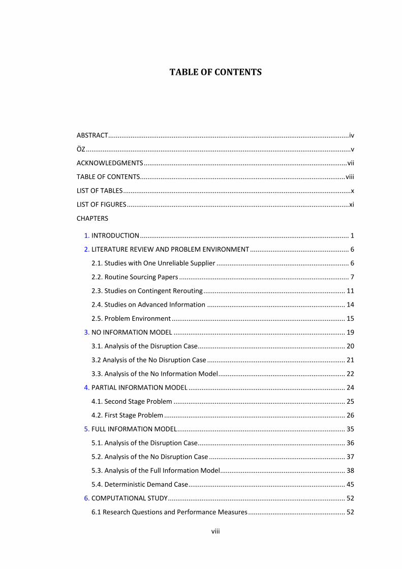
TABLE OF CONTENTS

ABSTRACT ................................................................................................................................. iv

ÖZ .............................................................................................................................................. v

ACKNOWLEDGMENTS ............................................................................................................. vii

TABLE OF CONTENTS .............................................................................................................. viii

LIST OF TABLES .......................................................................................................................... x

LIST OF FIGURES ....................................................................................................................... xi

CHAPTERS

1. INTRODUCTION ................................................................................................................ 1

2. LITERATURE REVIEW AND PROBLEM ENVIRONMENT ..................................................... 6

2.1. Studies with One Unreliable Supplier ....................................................................... 6

2.2. Routine Sourcing Papers ........................................................................................... 7

2.3. Studies on Contingent Rerouting ............................................................................ 11

2.4. Studies on Advanced Information .......................................................................... 14

2.5. Problem Environment ............................................................................................. 15

3. NO INFORMATION MODEL ............................................................................................ 19

3.1. Analysis of the Disruption Case ............................................................................... 20

3.2 Analysis of the No Disruption Case .......................................................................... 21

3.3. Analysis of the No Information Model .................................................................... 22

4. PARTIAL INFORMATION MODEL .................................................................................... 24

4.1. Second Stage Problem ............................................................................................ 25

4.2. First Stage Problem ................................................................................................. 26

5. FULL INFORMATION MODEL .......................................................................................... 35

5.1. Analysis of the Disruption Case ............................................................................... 36

5.2. Analysis of the No Disruption Case ......................................................................... 37

5.3. Analysis of the Full Information Model ................................................................... 38

5.4. Deterministic Demand Case .................................................................................... 45

6. COMPUTATIONAL STUDY ............................................................................................... 52

6.1 Research Questions and Performance Measures .................................................... 52

ix

6.2 Analysis of Parameter Sensitivity ............................................................................. 54

6.3 Analysis of Full Factorial Design ............................................................................... 71

7. CONCLUSION .................................................................................................................. 79

REFERENCES ........................................................................................................................... 82

APPENDICES

A PROOF OF COROLLARY 3.3.4 .......................................................................................... 84

B PROOF OF COROLLARY 3.3.5 .......................................................................................... 85

C PROOF OF COROLLARY 3.3.6........................................................................................... 86

D PROOF OF COROLLARY 3.3.7 .......................................................................................... 87

E PROOF OF COROLLARY 4.3.3 ........................................................................................... 88

F PROOF OF COROLLARY 4.3.4 ........................................................................................... 89

G THE OPTIMAL RESULTS FOR THE PARAMETER SENSITIVITY ANALYSIS .......................... 90

x

LIST OF TABLES

TABLES

Table 2.1 Summary of Conclusions of Tomlin (2006)…………………… …………………..….11

Table 2.2 Used Notations…………………………………………………………………………..…...…...18

Table 5.1 Summary of results on and in all models.........................................44

Table 5.2 Optimal & Values with Deterministic Demand……………………….………….49

Table 6.1: Base parameter set values…………………………………………………………….….....54

Table 6.2: Parameters values used for full factorial design………………………...…...…..71

Table 6.3 Max, Min, Average PoN Values………………………….……………………….………....73

Table 6.4 PoN values for different values….………………………………….……………...…..73

Table 6.5 PoN values for different values…………………………………….………..…74

Table 6.6 PoN values for different values..……………………….……………………..74

Table 6.7 Max, Min, Average FoP Values………………………………………..……………….…...76

Table 6.8 FoP values for different values…………………………………………………………..77

Table 6.9 FoP values for different values…………………..…..……………..….……..77

Table 6.10 FoP values for different values………….…………………………..….…..78

Table G.1: Optimal Results for the problem instances when is increased………...90

Table G.2: Optimal Results for the problem instances when is increased….….….91

Table G.3: Optimal Results for the problem instances when is increased…..….….92

Table G.4: Optimal Results for the problem instances when is increased…..….….93

Table G.5: Optimal Results for the problem instances when is increased…..…....94

Table G.6: Optimal Results for the problem instances when is increased.……..…95

xi

LIST OF FIGURES

FIGURES

Figure 2.1 Timeline of the Events…………………………………………………..........…..…........16

Figure 6.1 Optimal Profits when increases……………………………………………..…………56

Figure 6.2 Optimal Reservation Quantity when increases………………………..……….56

Figure 6.3 Optimal Order Quantity when increases…………….…………………………….57

Figure 6.4 PoN and FoP when increases………………………………………………….….….…58

Figure 6.5 Optimal Profits when increases………………………………………………..….…..59

Figure 6.6 PoN and FoP when increases………………………………………………….………..59

Figure 6.7 Optimal Reservation Quantity when increases…………….…………....…….60

Figure 6.8 Optimal Order Quantity when increases…………….….……………………..….60

Figure 6.9 Optimal Profits when increases………………………………………..…….….…....61

Figure 6.10 PoN and FoP when increases……………………………………………………..…..62

Figure 6.11 Optimal Reservation Quantity when increases…………………….….….….62

Figure 6.12 Optimal Order Quantity when increases…………………………..….….…….63

Figure 6.13 Optimal Profits when increases…………………………………………….…..…..64

Figure 6.14 PoN and FoP when increases………………………….………………………………65

Figure 6.15 Optimal Reservation Quantity when increases…………………….…..…….65

Figure 6.16 Optimal Order Quantity when increases…………….….……………….……..66

Figure 6.17 Optimal Profits when increases………………………………………………..…….67

Figure 6.18 PoN and FoP when increases…………………………..……………………..……..67

Figure 6.19 Optimal Reservation Quantity when increases…………….….…..…….….68

Figure 6.20 Optimal Order Quantity when increases…………….…………….…..……….68

Figure 6.21 Optimal Profits when increases……………………………………….…..………..69

Figure 6.22 PoN and FoP when increases……………………………………….……………..…70

Figure 6.23 Optimal Reservation Quantity when increases…………….…….…...…….70

xii

Figure 6.24 Optimal Order Quantity when increases…………….….………….……….….71

Figure 6.25 Average PoN values according to Problem Parameters……….……..….…75

Figure 6.26 Average FoP values according to Problem Parameters………….……...….78

1

CHAPTER 1

INTRODUCTION

A company should specify and mitigate uncertainties that exist in its supply chain

system in order to meet customer needs. Supply uncertainty is one of the most

important difficulties to the firms on meeting customer needs. Traditional inventory

models consider demand uncertainty and show how to design supply chain systems

to mitigate that risk. However, the effects of supply uncertainty can have serious

detriments against design and during production, possibly more than demand

uncertainty can have. Recent studies in supply chain literature have begun to

consider supply uncertainty as a major topic. Real life events and theoretical studies

both demonstrated its impacts in supply chains when firms fail to protect or

mitigate against it.

Supply uncertainty can occur in several forms. Disruptions, yield uncertainty,

capacity uncertainty, lead time uncertainty, input cost uncertainties are the main

forms of supply uncertainty. Disruptions are random events that cause a supplier to

stop producing completely. That is, the supplier cannot produce any product during

a disruption. Yield uncertainty is the event when the supplier cannot send all

amount of the quantity ordered, it sends partial amount of the quantity ordered.

The quantity sent is stochastic, which can be independent of or proportional to the

order quantity in an additive or multiplicative fashion. So, it can be said that

disruption is a special case of yield uncertainty when the quantity sent is equal to

zero. This thesis considers all-or-nothing supply. Like the other analytical models,

2

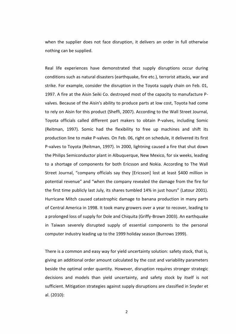
when the supplier does not face disruption, it delivers an order in full otherwise

nothing can be supplied.

Real life experiences have demonstrated that supply disruptions occur during

conditions such as natural disasters (earthquake, fire etc.), terrorist attacks, war and

strike. For example, consider the disruption in the Toyota supply chain on Feb. 01,

1997. A fire at the Aisin Seiki Co. destroyed most of the capacity to manufacture P-

valves. Because of the Aisin's ability to produce parts at low cost, Toyota had come

to rely on Aisin for this product (Sheffi, 2007). According to the Wall Street Journal,

Toyota officials called different part makers to obtain P-valves, including Somic

(Reitman, 1997). Somic had the flexibility to free up machines and shift its

production line to make P-valves. On Feb. 06, right on schedule, it delivered its first

P-valves to Toyota (Reitman, 1997). In 2000, lightning caused a fire that shut down

the Philips Semiconductor plant in Albuquerque, New Mexico, for six weeks, leading

to a shortage of components for both Ericsson and Nokia. According to The Wall

Street Journal, “company officials say they [Ericsson] lost at least $400 million in

potential revenue” and “when the company revealed the damage from the fire for

the first time publicly last July, its shares tumbled 14% in just hours” (Latour 2001).

Hurricane Mitch caused catastrophic damage to banana production in many parts

of Central America in 1998. It took many growers over a year to recover, leading to

a prolonged loss of supply for Dole and Chiquita (Griffy-Brown 2003). An earthquake

in Taiwan severely disrupted supply of essential components to the personal

computer industry leading up to the 1999 holiday season (Burrows 1999).

There is a common and easy way for yield uncertainty solution: safety stock, that is,

giving an additional order amount calculated by the cost and variability parameters

beside the optimal order quantity. However, disruption requires stronger strategic

decisions and models than yield uncertainty, and safety stock by itself is not

sufficient. Mitigation strategies against supply disruptions are classified in Snyder et

al. (2010):

3

1) Inventory: Extra inventory can be held so as to meet some critical

customer’s need during a disruption if the firm does not apply any other

strategy like backup supplier option. However, as it is mentioned before only

extra inventory cannot be the solution to supply disruption.

2) Diversification in Sourcing

i) Routine Sourcing: Firms regularly source raw materials from more

than one supplier. If one supplier faces disruption, the firm is not left

completely without products since the other supplier(s) may still be

up. Ordering process from either supplier or suppliers is done at the

beginning and at the same time for all suppliers. Order quantity

decision is made for each supplier and order quantities to the non-

disrupted suppliers cannot be changed after a disruption occurrence

in any supplier.

ii) Contingent Sourcing: It is almost the same as routine sourcing.

However, in the case of contingent sourcing, if one supplier faces

disruption, the order from the non-disrupted suppliers can be

changed from the pre-disruption levels.

3) Information Sharing: It is obtaining and assessing information about the

disruption risk of suppliers. It can be achieved by monitoring suppliers to

anticipate potential disruptions and adopt better strategies.

4) Demand Substitution: If one product of a supplier faces disruption, the firm

can introduce an inferior product with decreased price or superior product

with the same price.

5) Financial Mitigation: Firms may purchase some insurance to protect from

disruptions.

4

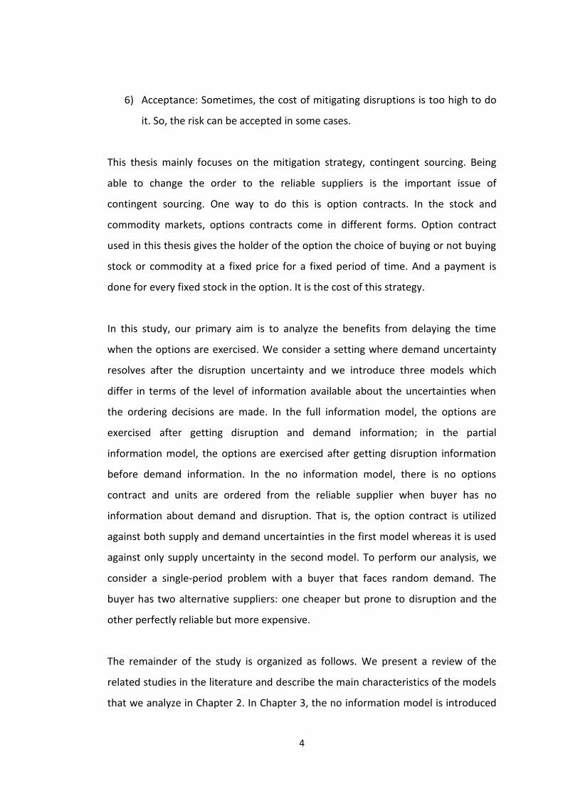
6) Acceptance: Sometimes, the cost of mitigating disruptions is too high to do

it. So, the risk can be accepted in some cases.

This thesis mainly focuses on the mitigation strategy, contingent sourcing. Being

able to change the order to the reliable suppliers is the important issue of

contingent sourcing. One way to do this is option contracts. In the stock and

commodity markets, options contracts come in different forms. Option contract

used in this thesis gives the holder of the option the choice of buying or not buying

stock or commodity at a fixed price for a fixed period of time. And a payment is

done for every fixed stock in the option. It is the cost of this strategy.

In this study, our primary aim is to analyze the benefits from delaying the time

when the options are exercised. We consider a setting where demand uncertainty

resolves after the disruption uncertainty and we introduce three models which

differ in terms of the level of information available about the uncertainties when

the ordering decisions are made. In the full information model, the options are

exercised after getting disruption and demand information; in the partial

information model, the options are exercised after getting disruption information

before demand information. In the no information model, there is no options

contract and units are ordered from the reliable supplier when buyer has no

information about demand and disruption. That is, the option contract is utilized

against both supply and demand uncertainties in the first model whereas it is used

against only supply uncertainty in the second model. To perform our analysis, we

consider a single-period problem with a buyer that faces random demand. The

buyer has two alternative suppliers: one cheaper but prone to disruption and the

other perfectly reliable but more expensive.

The remainder of the study is organized as follows. We present a review of the

related studies in the literature and describe the main characteristics of the models

that we analyze in Chapter 2. In Chapter 3, the no information model is introduced

5

and analyzed. Chapter 4 includes the partial information model and Chapter 5

includes the full information model. To gain insights on the value of delaying the

time when options are exercised, we perform a thorough computational analysis in

Chapter 6. Finally, we conclude in Chapter 7 summarizing our major findings and

offering further research directions.

6

CHAPTER 2

LITERATURE REVIEW AND PROBLEM ENVIRONMENT

This paper contributes to the important and growing research area of supply

disruptions management. Dual sourcing mitigation strategy with options contract is

used against the supply uncertainties. Supply disruption is a form of yield

uncertainty so we first analyze the papers with only yield uncertainty and both of

them, then the papers with only supply disruption in the literature review. We also

look at how the papers that work on single sourcing mitigate supply uncertainties.

2.1. Studies with One Unreliable Supplier

Supply uncertainty was generally modeled as complete disruptions, where supply

stops completely, or as yield uncertainty, where the supply quantity received varies

stochastically. Early on, papers focusing on supply uncertainty usually consider

single-supplier systems. (see for instance Bielecki and Kumar 1988, Parlar and

Berkin 1991, Parlar and Perry 1995, Gupta 1996, Song and Zipkin 1996, Moinzadeh

and Aggarwal 1997, Parlar 1997, Arreola-Risa and De Croix 1998, Schmitt, et al.

2010).Bielecki and Kumar (1988) shows that a policy similar to a zero inventory

ordering policy is sometimes optimal for an unreliable supply chain system,

contradicting the common belief that inventories are always valuable for buyers in

uncertain environments. Parlar and Berkin (1991) is the first study that introduces

disruption into the EOQ model. On and off periods of disruption have random

lengths. They conclude that cost function is convex according to disruption on and

7

off periods. Parlar and Perry (1995) extends EOQ model with disruption by allowing

the reorder point to be a decision variable. Yano and Lee (1995) provide a literature

review on quantitatively oriented approaches for determining lot sizes when

production or supply yields are random. One of the latest papers, Schmitt, et al.

(2010) considers three cases: (i) disruption, deterministic demand and deterministic

supply yield, (ii) disruption, deterministic demand and stochastic supply yield and

(iii) disruption, stochastic demand and deterministic supply yield. They find optimal

base-stock inventory policies in a multi-period setting. There is always one

unreliable supplier that is prone to disruptions. The objective is to find the

parameters that make the service level maximum (minimum holding/penalty cost).

Everything is deterministic in case (i), so if the firm decides to carry no safety stock,

disruption would have the largest detrimental effect on the supply chain system. In

the no disruption case and with equal standard deviation (either on the demand or

the supply yield), cases (ii) and (iii) would stock the same safety stock quantity.

Therefore they would be equally affected by disruptions. In this paper, it is

concluded that the safety stock is maintained to compensate variability from

demand or yield. Because, in a disruption case if the disruption lasts not short, all

cases shortage as quantity of demand so disruptions should be mitigated regardless

of other variability, demand or yield.

2.2. Routine Sourcing Papers

There is a growing body of literature that uses routine sourcing as a strategy to

mitigate disruption risk. In routine sourcing, the buyer orders from multiple

suppliers in the beginning and at the same time.

Anupindi and Akella (1993) study dual sourcing with unreliable suppliers. Different

combinations of disruption and yield uncertainty result in three models. Each model

has a single and a multi-period version. The first model assumes a delivery contract

with each supplier that the supplier delivers a given order either in the current

8

period with a given probability 1- , or in the next period with probability , when

disruption occurs. It delivers nothing in the single period case when disruption

occurs. The second and the third models consider yield uncertainty as well. Demand

is stochastic and has a continuous distribution. The objective is to find the optimal

orders from both suppliers that minimize the ordering, holding and penalty costs.

They prove that the optimal ordering policy has three regions, based on the current

on-hand inventory. Order nothing (if on-hand inventory is large enough), order only

from the less expensive supplier (if on-hand inventory is moderate), and order from

both suppliers (if on-hand inventory is small). Anupindi and Akella (1993) shows

that the buyer should never order from the expensive supplier alone. Swaminathan

and Shanthikumar (1999) study Anupindi and Akella's first model and show that,

when the demand is deterministic, their ordering policy is no longer optimal.

Swaminathan and Shanthikumar (1999) proved that ordering from only expensive

supplier is a possible optimal solution. They also provide necessary conditions under

which it is optimal to order at least some units from the more expensive supplier.

Lakovou et al. 2009 consider a single period supply chain system that consists of a

manufacturer and two unreliable suppliers which are both prone to disruptions,

such as production, transportation and security-related disruptions. They propose a

single period system where a single ordering decision from both suppliers is to be

made at the beginning of the period in order to maximize expected total profit.

Disruption is modeled as each disruption may occur only once for each of the two

suppliers, during the period with a probability. Furthermore, when a disruption

occurs it is assumed that a constant percentage of the order quantity will be

available in time to satisfy the demand during the period and the remaining

quantity will be delivered at the end or after the end of the period.

There are also papers that use routine sourcing strategy with multiple (more than

two) unreliable suppliers: See for instance Dada et al. 2007, Federgruen and Yang

2008, Federgruen and 2009, Tehrani et al. 2010. Dada et al. (2007) study a single-

9

period model with multiple unreliable suppliers. The objective is to choose which

suppliers to order from and in what quantities in order to maximize the expected

profit (sales and salvage revenues minus holding and stock-out costs). Disruptions,

yield uncertainty, and capacity uncertainty are all special cases in this paper.

Demand is stochastic, with a continuous distribution. Two extensions about capacity

uncertainty are studied in the paper. In the first extension, there exist multiple

suppliers and each supplier's capacity is deterministic. In this case, the newsvendor

orders as much as possible from the least expensive supplier. If the capacity of the

least expensive supplier is not enough, then it orders as much as possible from the

second least expensive supplier and so on. In the second extension, there exists

only one supplier capacity of which is uncertain. In other words, it is not guaranteed

that to receive amount ordered from the supplier. In this case, the newsvendor

should order no less than the amount that would have been ordered from the

supplier if the supplier’s capacity were deterministic. From the two cases, a major

conclusion is that if a supplier is not chosen, then suppliers that are no more

expensive than that supplier will be used whatever the reliability degree is. That is,

cost trumps reliability. This result is parallel to the solution of Anupindi and Akella

(1993). Another conclusion is: if a given supplier is reliable, then no more expensive

suppliers than that reliable supplier will be used. They also show that the optimal

order quantity is larger and the optimal service level is smaller with unreliable

suppliers than it is for the classical newsboy problem. Because the variability in the

demand is the same with the classical newsboy problem but the variability in the

supply, capacity is extra and it is detrimental for the service level.

The model of Federgruen and Yang (2008) and Federgruen and Yang (2009) is

similar to Dada et al. (2007). The suppliers are subject to yield uncertainty in the

form of multiplicative yield with a general yield distribution. Disruptions are special

case of yield uncertainty. Federgruen (2009) makes a modification of their 2008

model in design of cost model. The supply model is the same. In both study, they

define a key quantity as “expected effective supply” that is the total expected yield

10

from all suppliers. They find that total cost is a convex function of expected

effective supply. In addition, they conclude that when the suppliers are sorted in

increasing order of their per-unit costs divided by their yield factors, optimal

suppliers include the first suppliers, for some .

Tehrani et al. (2010) consider a two-echelon inventory system with multiple

unreliable suppliers. Suppliers are prone to common source disruptions so their

production capacity (delivery quantities) is stochastically dependent. This is the

extra uncertainty considered by Tehrani et al. (2010) in addition to Dada et al.

(2007)’s uncertainties. It considers a single-period model. Two cases are studied,

namely, the multi-source and assembly supply chains. In the multi-source structure,

suppliers produce and send the same product to the buyer. In the assembly

structure, each supplier produces a different part of the product, so the end units

manufactured by the buyer equal the minimum of the supplier’s order delivery

quantity. For each supply chain structure, the objective is to search the impact of

the dependence in capacities, induced by common-source disruptions, on the

important performance measures of the buyer such as service level and to find the

optimal ordering policy. They conclude that the stochastic dependence between

suppliers’ disruption probability has opposite impacts on the system in the two

structures: total disruption risk of the assembly system increases as the level of

dependence increases in the multi-source supply chain. Furthermore, as disruption

risks become more dependent, the buyer should order less in the multi-source

supply chain but order more in the assembly supply chain.

Berger et al. (2004), Ruiz-Torres and Mahmoodi (2007) investigate the optimal

number of suppliers to use from a number of unreliable suppliers. Berger et al.

(2004) assume an operating cost that is a function of number of used suppliers.

Another special cost is the fixed penalty cost when all of the used suppliers disrupt

simultaneously. Ruiz-Torres and Mahmoodi (2007) study a similar model with

Berger et al. (2004) but one thing is different: the fixed penalty cost is incurred

11

when only some suppliers disrupt. The main conclusion of these papers is that

optimal number of unreliable suppliers used is small generally.

2.3. Studies on Contingent Rerouting

Papers that study supply disruptions that used contingent sourcing as a mitigation

strategy emerged in the literature recently. The basic idea of the contingent

sourcing strategy briefly is: if one supplier disrupts, the order from the non-

disrupted suppliers can be changed from the pre-disruption levels. We consider

such papers in more detail as our work also invokes contingent rerouting.

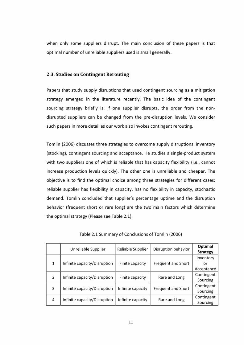
Tomlin (2006) discusses three strategies to overcome supply disruptions: inventory

(stocking), contingent sourcing and acceptance. He studies a single-product system

with two suppliers one of which is reliable that has capacity flexibility (i.e., cannot

increase production levels quickly). The other one is unreliable and cheaper. The

objective is to find the optimal choice among three strategies for different cases:

reliable supplier has flexibility in capacity, has no flexibility in capacity, stochastic

demand. Tomlin concluded that supplier’s percentage uptime and the disruption

behavior (frequent short or rare long) are the two main factors which determine

the optimal strategy (Please see Table 2.1).

Table 2.1 Summary of Conclusions of Tomlin (2006)

Unreliable Supplier Reliable Supplier Disruption behavior Optimal Strategy

1 Infinite capacity/Disruption Finite capacity Frequent and Short Inventory

or Acceptance

2 Infinite capacity/Disruption Finite capacity Rare and Long Contingent

Sourcing

3 Infinite capacity/Disruption Infinite capacity Frequent and Short Contingent

Sourcing

4 Infinite capacity/Disruption Infinite capacity Rare and Long Contingent

Sourcing

12

Chopra et al. (2007) study a single-period model in which one supplier is subject to

both yield and disruption uncertainties and the other is perfectly reliable. In

contrast to Tomlin’s models, both yield and disruption uncertainties are unresolved

when the buyer places an order to the first supplier. This model also requires the

buyer to reserve a maximum order size with the reliable supplier at a given

reservation price. When order comes from the first supplier, the buyer can exercise

up to the reservation quantity (maximum order size) from the reliable supplier if

demand cannot be met from the first supplier’s delivery. This paper assumes

demand is deterministic. The objective is to find the utilization proportion of

reliable and unreliable suppliers in different situations: for example decoupling risks

with disruption and yield uncertainty, increasing disruption probability etc.

Conclusions of this paper expand Dada’s conclusions by separately considering

whether the supply risk is yield uncertainty or because of disruption. When the

increase in supply uncertainty is from an increase in yield uncertainty, increased use

of the cheaper supplier is optimal. When the increase in supply uncertainty is from

disruption, increased use of reliable supplier is optimal. In this paper, it is concluded

that reliability trumps cost.

Schmitt and Snyder (2009) claim that disruptions have a significant impact on future

periods, and planning for these disruptions can have a significant impact on order

quantities of all periods. They also claim that one-period models are suitable for the

perishable product systems or the systems that disruptions last relatively short.

They extend Chopra et al. (2007) to a multi-period setting. Multi-period and single-

period models’ solutions are compared and it is concluded that a single-period

approximation causes increases in cost, under-utilization of unreliable supplier, and

spoils order quantities that is to be placed to the reliable supplier.

Qi (2009) develops a model different than the standard contingent rerouting. There

are two suppliers one of which is reliable the other one is unreliable. In the

standard contingent sourcing models, when unreliable supplier disrupts, the buyer‘s

13

only option is to order immediately from the reliable supplier. Qi (2009) considers

another option: in a disruption case the buyer can wait a while up to the unreliable

supplier recovers itself. In contrast to Qi’s model, in our models, there is no such a

chance that in a disruption case the buyer can wait a while up to the unreliable

supplier recovers itself. Demand is considered as deterministic in Qi(2009).

Disruption duration is distributed exponentially. In the model, the duration that the

buyer waits before ordering from the reliable supplier is a decision variable. In this

multi-period setting, the buyer follows an (s, S) type review policy, with different S

values depending on from which supplier order is set. Qi (2009) concluded that it is

always optimal for the firm to either order from the reliable supplier immediately

after the safety stock runs out or wait as long as necessary until the unreliable

supplier recovers.

Hou et al. (2010) consider a two-stage supply chain with dual sourcing system.

There are two suppliers one of which is main supplier that prone to disruptions,

other one is back-up supplier with which the buyer can sign a buy-back contract.

They consider two types of risk, namely disruption risk which results in a zero

delivery and yield uncertainty which is reflected in an uncertain delivery volume.

Some papers study contingent sourcing and try to evaluate the value of advance

warnings of disruptions. It is the comparison of the cases whether the exact time of

disruption, disruption duration or the probability of disruption is known or not.

Snyder and Tomlin (2008) investigate how inventory systems can be designed to

take advantage of advanced information of disruptions. They consider a system

with an unreliable supplier that is subject to complete disruptions and a reliable

supplier that is perfectly reliable. The disruption profile can change over time.

Advance information of disruption means that buyer is informed about disruption

characteristics continuously, which constitute what Snyder and Tomlin call “threat

level”, change stochastically over time, and the buyer knows the current threat level

14

continuously. They model the system using a discrete-time Markov chain for the

disruption distribution where states correspond to threat levels for disruption. The

main conclusion is that advanced information is extremely beneficial and allows

superb cost savings especially when the disruption probabilities are significantly

different in different states. Another conclusion is that the benefit of the advanced

information decreases as the capacity decreases.

2.4. Studies on Advanced Information

Saghafian and Van Oyen (2011) investigate two significant remedies to increase

supply chain effectiveness. First one is contracting an option contract with a reliable

supplier that can produce two products but having a shared capacity for two

products. Second one is obtaining advanced disruption information as an extra

mitigation strategy. There are two products and two unreliable suppliers of them.

There is one reliable backup supplier that can produce both products. However, this

supplier is more expensive than others. The option contract is done with this

reliable backup supplier: the buyer pays a fixed reservation price to the supplier at

the beginning of the contract in return for the delivery of any desired portion of the

reserved shared capacity for two products at an additional purchasing price. In

other words, the reliable supplier can mitigate the risk of disruption in unreliable

suppliers while reducing the cost of keeping excess inventory. Demand for both

products is stochastic. The problem is studied in a single period context. The

objective is to find optimal values of order quantities from unreliable suppliers and

capacity reserved from the reliable supplier in the first remedy. Comparing and

valuing advanced information of disruption is the objective in the second remedy. It

is observed that investing in a reliable backup capacity can be detrimental if the

advanced information about the disruption risk of unreliable suppliers is not

perfect. Monitoring unreliable suppliers to obtain better disruption estimates

increases the benefit of reserving reliable backup capacity. Additionally, advanced

information about disruption risk is more valuable to firms with low profit margins

15

than those with high ones. They also showed that when suppliers are (truly) reliable

enough, obtaining information is a better mitigation strategy than contracting with

a reliable supplier. Another conclusion is that when unreliable suppliers are reliable

enough, contracting with an expensive reliable supplier is not advantageous.

However, obtaining advanced disruption risk information is still advantageous

because it helps the firm to make better ordering decisions.

Our first model is closely linked to the work of Saghafian and Van Oyen (2011)’s

single product special case. Our partial information model distinguishes from this

work and the literature about the advanced information part. Saghafian and Van

Oyen (2011) study to value advanced information of disruption risk information.

However, we study to value advanced information of demand and disruption both.

2.5. Problem Environment

We consider a two-stage supply chain consisting of a single buyer and two suppliers

one of which is unreliable and prone to disruption whereas the other is perfectly

reliable. When disruption occurs, supply from the first supplier is zero. The buyer

faces stochastic demand in a single period, which is modeled as a continuous

random variable having nonnegative support (The notation is presented in Table

2.2). Contingent rerouting mitigation strategy is adopted in our paper. The buyer

has a wholesale-price only contract with the unreliable supplier and options

contract with the reliable supplier. The options contract provides flexibility to the

supplier against uncertainties in the system.

In our models, disruption and demand uncertainties are unresolved when the buyer

places an order to the unreliable supplier. In the first model, disruption and demand

uncertainties are unresolved when the buyer places order from the reliable supplier

similar to unreliable supplier. In other words, there is no options contract. We call

this model as “No Information Model”. In the second model, option-exercise takes

16

place after supply disruption information is received but before demand uncertainty

is not resolved. Hence, we call this model as “Partial Information Model”. When

both uncertainties are resolved, the buyer can exercise up to the reserved amount

from the reliable supplier if demand cannot be met from the first supplier’s

delivery. We call this model as “Full Information Model”. Please see Figure 2.1 for

the timeline of events for each model.

A) No Information Model

B) Partial Information Model

C) Full Information Model

Figure 2.1 Timeline of Events

Order Q, Order I

Getting disruption

information

Getting units from suppliers

Getting demand

information

Demand realizes

Order Q, Reserve I

Getting disruption

information

Option-Exercise

Getting demand

information

Demand realizes

Order Q, Reserve I

Getting disruption

information

Getting demand

information

Option-Exercise

Demand realizes

17

In all models, the cost of reserving plus exercising one unit of product from the

reliable supplier is higher than the cost of buying one unit of product from the

unreliable supplier, . Otherwise, the buyer would never use the unreliable

supplier. Revenue earned from one unit is bigger than cost incurred from one unit

in both supplier, and . We assume that there is no salvage value and

loss sales cost although these can be easily incorporated into our models.

Our study makes a key contribution to the literature in that option contract can be

used only against disruption uncertainty. In our partial information model, demand

is realized after the buyer exercises options from the second supplier. Hence, the

options contract becomes an action against only the disruption uncertainty. It does

not mitigate demand uncertainty because demand uncertainty has not resolved yet

when options are exercised. However, both uncertainties are resolved when

options are exercised in our full information model. By this way, we study the value

of advanced demand information via comparison of two models. The difference

between two models is whether the buyer exercises options before getting

information on demand or not. So, profit difference between two models is

considered as the value of deciding how many to exercise with demand

information.

18

Table 2.2 Used Notations

X Random variable representing customer demand

f(x) Probability density function (p.d.f) of random variable X

F(x) Cumulative distribution function (c.d.f) of random variable X

Y Bernoulli random variable representing supply disruption where Y = 1

denotes supply disruption and Y = 0 denotes otherwise.

Q Order quantity from the unreliable supplier

Reservation quantity from the reliable supplier

p First supplier disruption probability

c Cost per unit from the first supplier

h Cost per unit reserved from the second supplier

e Cost per unit exercised from the second supplier

r Revenue per unit

19

CHAPTER 3

NO INFORMATION MODEL

In the no information model, the buyer makes order decisions from both suppliers

in a situation that he knows nothing; he doesn't know disruption occurrence

information and demand uncertainty has not resolved yet. This model aims to

generate insights about a two supplier supply chain system; one of them is cheap

but unreliable, the other is reliable but expensive. There is no option contract in

other words there is no option to exercise after the uncertainties resolved. Buyer

has to decide how many units to order (exercise) from the reliable supplier at the

beginning. The sequence of events in this setting is as follows:

1. The buyer orders units from the first supplier and orders I units from the

second supplier.

2. The buyer gets disruption information about the first supplier.

3. The buyer gets units from the second supplier, units from the first

supplier if disruption doesn’t occur.

4. The buyer gets full information about demand.

5. Demand realizes.

6. The buyer satisfies the demand.

The buyer’s objective is to maximize its expected profit. To characterize its expected

profit, we work on order quantities from the two suppliers. As the uncertainty in

20

supply is discrete, we examine each case (disruption and no disruption) separately.

After that we take expectation with respect to random variable Y (supply

disruption) to get the expected profit.

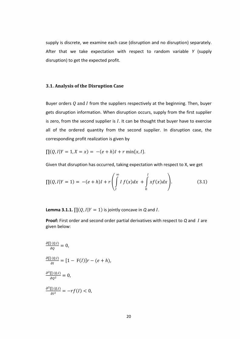
3.1. Analysis of the Disruption Case

Buyer orders from the suppliers respectively at the beginning. Then, buyer

gets disruption information. When disruption occurs, supply from the first supplier

is zero, from the second supplier is . It can be thought that buyer have to exercise

all of the ordered quantity from the second supplier. In disruption case, the

corresponding profit realization is given by

| { }.

Given that disruption has occurred, taking expectation with respect to X, we get

| (∫

∫

)

Lemma 3.1.1. | is jointly concave in Q and .

Proof: First order and second order partial derivatives with respect to Q and are given below:

[ ] ,

21

= 0.

Determinant of the Hessian matrix is:

(

) (

) (

)

Hence, | is jointly concave in Q and .

3.2 Analysis of the No Disruption Case

When disruption does not occur, supply from the first supplier is , from the

second supplier is . In the no disruption case, the corresponding profit realization is

given by

| { } .

Given that disruption has not occurred, taking expectation with respect to X, we get

|

(∫

∫

)


Proof: First order and second order partial derivatives with respect to Q and are shown below:

[ ] ,

[ ] ,

,

,

22

Determinant of the Hessian matrix is given as follows:

(

) (

) (

)


3.3. Analysis of the No Information Model

In this section, we formulate and analyze the no information model by combining

the results of Section 3.1 and Section 3.2. Utilizing Equation (3.1) and Equation (3.2),

and taking expectation with respect to Y, the expected profit of the buyer can be

characterized as

[ (∫

∫

)]

[ (∫

∫

)]

Then, the buyer’s problem is

Max

Subject to Q, ≥ 0.

Let ( denote the optimal order (reservation) quantity from the unreliable

(reliable) supplier. Then, the following theorem characterizes the optimal solution

to the buyer’s problem.

23

Theorem 3.3.1. If , then and

(

). Otherwise, [

] and

(

) .

Proof: We have shown that | and | are jointly concave in

Lemma 3.1.1 and Lemma 3.2.1; hence, the objective function is strictly concave.

Also, constraints are linear. There exists a unique optimal solution to the

unconstrained problem and it is given by the unique solution to

and

. From

, we have [

] and from

we have (

) . when [

] .

Otherwise, inequality constraint becomes binding and determines optimal solution

as Hence, we can argue that, when ,

and (

), which completes the proof.

24

CHAPTER 4

PARTIAL INFORMATION MODEL

In the partial information model, buyer makes exercise decision from the second

supplier in a situation that he only has disruption occurrence information and

demand uncertainty has not resolved yet. Options contract is available and the

buyer can reserve at the beginning and exercise after demand uncertainty is

resolved. This model aims to generate insights about option contract management

when it is settled only for disruption uncertainty; in other words option contract is

used to mitigate only disruption uncertainty. Demand uncertainty still stays as a risk

factor for the system when option contract is used. The sequence of events in this

setting is as follows:

1. The buyer orders Q units from the first supplier and reserves I units from the

second supplier.


3. The buyer determines the number of options to exercise, .


5. Demand realizes.

6. The buyer satisfies the demand.


profit, we consider a two-stage problem setting. We work backwards and start with

the second stage problem which is to determine the optimal exercise quantity, E.

25

Then, we continue with the first stage problem to characterize the optimal order

quantity Q, and, reservation quantity, , from the associated suppliers.

4.1. Second Stage Problem

The second stage problem is to determine the optimal number of options to

exercise given the condition of the first supplier. It should be noted that the order

and reservation quantities are fixed at this stage. Hence, only relevant costs and

revenues are the unit revenue, r, and unit cost of exercising an option, e.

The second stage problem is actually the same as newsvendor problem where the

number of copies of the day's paper to stock is determined in the face of uncertain

demand and knowing that unsold copies will be worthless at the end of the day. In

our problem, the decision of how many newspapers to stock corresponds to the

decision of how many to exercise from the second supplier. Demand is uncertain

and both decisions are made before demand realization. Buyer knows how many he

already has (in no disruption we have , in disruption we have zero.) So, we can

write the optimal exercise quantity for each case (disruption and no disruption)

which maximizes the expected profit as the same with newsvendor problem. The

buyer faces only uncertain demand and demand distribution, revenue, unit cost are

the factors that influence the exercise decision.

Given that disruption has occurred ( ), the buyer faces a capacitated

newsvendor problem and the corresponding optimal number of options to exercise

is given by ( | { (

) }.

Given that disruption has not occurred ( ); the buyer’s problem is

{ | } where | [ { }] . The

problem is quite similar to the newsvendor problem and the optimal number of

options to exercise is { { (

) }}.

26

4.2. First Stage Problem

We start the analysis of the first stage problem by characterizing the expected profit

of the buyer given the condition of the first supplier. After that, taking expectation

with respect to Y, we characterize the expected profit in the first stage as a function

of and

Let (

). Given that disruption has occurred and recalling that

( | { }, the expected profit is

|

∫

{ }

∫ { } { }

{ }

Given that disruption has not occurred (Y=0) and taking expectation with respect to

X, the expected profit is

| ∫

∫

where { { }}.


(reliable) supplier. Then, following Lemma simplifies the buyer’s problem.

Lemma 4.2.1.The optimal reservation quantity cannot exceed (

).

Proof: In the analysis of the second stage problem (Section 4.1), we have shown

that the optimal number of options to exercise will never exceed A. Then, we can

27

deduce that the options reserved in excess of A will never be utilized. Hence, it is

never optimal to reserve more than A.

We can now characterize the expected profit of the buyer in the first stage. Due to

Lemma 4.2.1, we have

(∫

∫

)

{

where

∫

∫

∫

∫

∫

∫

Then, the buyer’s problem can be formulated as

Max

subject to

28

Lemma 4.3.1. is continuously differentiable.

Proof: For continuity, it is sufficient to check the breakpoints and .

For , we evaluate and , and observe that

∫

∫

Hence, is continuous at the points .

For , we evaluate and , and observe that

∫

∫

Hence, is continuous at the points which completes the proof for

continuity.

For differentiability, the first derivatives of with respect to and are

given below:

{

( )

( )

[ [ ] ]

{

[ [ ] ]

It is sufficient to check the breakpoints and .

29

At points , we evaluate

,

and observe that

since

due to the definition of A.


,

and observe that

since

due to the definition of A. Hence, is

differentiable at the points .


,

and observe that

since

due to the definition of A. Hence, is

differentiable at the points , which completes the proof.

Theorem 4.3.3. For a given , if , then (

). Otherwise,

{ (

) }.

Proof: We consider the case first. For ,

[ ] since and . For ,

. Hence, should be in the region (A,∞). For ,

[ ] . Setting

, we get

(

) since .

Next we consider the case . For , we have [ ]

since and . For ,

. Hence

should be in the region [ ]. For ,

[

] . Setting

, we get (

) . Then,

{ }

30

Theorem 4.3.4. For a given , if [ [ ] ]

, then Otherwise, if [

] (

) , then [

]

otherwise, is given by the unique solution to [ [ ] ]

[ [ ] ]

Proof: Consider the case where [ [ ] ] .

Then, for ,

and

Hence, is

decreasing in for . For ,

. Since the derivative is

continuous, is decreasing in for .

Hence, ( if [ [ ] ] .

Now, consider the case where [ [ ] ] . For

,

[ [ ] ].

Setting

, we get [

] If , then it is the optimal

solution. Otherwise the optimal solution is in the region and can be

obtained by

.

Theorem 4.3.5 For a given , if then . Otherwise,

[

]

Proof: Given ,

[ [ ] ].

31

If ,

hence Otherwise since

, we set

, which completes the proof.

Corollary 4.3.1. The optimal order and reservation quantities under partial

information are given by:

(i) If , (

), {

[

]

(ii) If ,

{( (

) )

(

) [

] [

]

Proof: If , the optimal order and reservation quantities directly follow from

Theorem 4.3.3 and Theorem 4.3.5.

We next consider the case with . If , we

have [ ] for all (

). From

Theorem 4.3.3, we have (

) . Hence, we have and

is given by [ [ ] ] [ [ ] ] (4.10)

Since (

), Equation (4.10) reduces to

which results in [

]

For , consider the candidate solution

( (

) ) From Theorem 4.3.3, we have (

) and

satisfies it. since . For , we have

[ ] . Hence from Theorem 4.3.4, we have and (

32

satisfies it. Since satisfy the optimality conditions in Theorem 4.3.3 and 4.3.4,

we can conclude that it is optimal.

This corollary demonstrates that optimal order quantity is always greater than zero

in partial information as it is in full information with stochastic demand. This is

because cost per unit from the first supplier is always less than the second supplier.

Buyer always wants to buy from the cheaper supplier and compensate the

disruption risk of the cheaper supplier with the option contract.

Expected profit per unit if the buyer uses second supplier rather than first supplier

is when , otherwise it is .

Buyer earns for one exercised unit in disruption case because there is no

opportunity other than using second supplier, in no disruption case because

there is an opportunity to supply from the first supplier so opportunity cost of using

second supplier rather than first supplier, . We take expectation according to Y

and the expected profit becomes . However, in no

disruption case buyer always use first supplier when because he doesn’t want

to give more money when he has an opportunity to supply from the first supplier.

Hence, expected profit per unit is when .


{

If this profit is positive in either case, buyer always reserves from the second

supplier. Otherwise, he reserves nothing.

This condition that makes buyer not reserve from the second supplier are the same

as in full information with deterministic demand. We realize that buyer reserves

nothing in the same condition even if buyer doesn’t get demand information and

demand is uncertain while exercising from the second supplier.

33

Total amount of units ordered or reserved, , converges to (

) except

when and . In this exception case, (

).

This result is quite similar to the optimal solution of full information model with

deterministic demand. Total amount of units ordered or reserved converges to

demand quantity, D, except when and on full information

with deterministic demand. In this exception case .

Corollary 4.3.2. ( ) is non-increasing (non-decreasing) in the unit cost, c

Proof: From corollary 4.3.1, we have two different alternatives solution to ; for

, (

) [

] which

can be written as (

) [

], otherwise

{ (

) }. In either case, we can argue that is non-increasing in

the unit cost, c. From corollary 4.3.1, we have two different alternative solutions to

, for , max{ [

] } and for ,

max{ [

] } which can be written as max{ [

] } .

In either case, we can argue that is non-decreasing in the cost, c, which

completes the proof.

Corollary 4.3.3. ( ) is non-decreasing (non-increasing) in the reservation cost, h

and exercise price, e.

Proof: The proof is similar to the proof of Corollary 4.3.2 and it is presented in

Appendix E.

34

Corollary 4.3.4. ( ) is non-increasing (non-decreasing) in the disruption

probability, p


Appendix F.

35

CHAPTER 5

FULL INFORMATION MODEL

In the full information model, we assume the buyer makes the decision of how

many products to exercise from the second supplier in an environment that he

knows everything about the uncertain matters, disruption occurrence or not

occurrence and demand uncertainty. The order of events is as follows:

1. The buyer orders Q units from the first supplier and reserves I units from the

second supplier.



4. The buyer orders units from the second supplier.

5. Demand realizes.


profit, we work backwards and start with the optimal exercise quantity, E. As the

uncertainty in supply is discrete, we examine each case (disruption and no

disruption) separately. After that we take expectation with respect to random

variable Y (supply disruption) to get the expected profit.

36

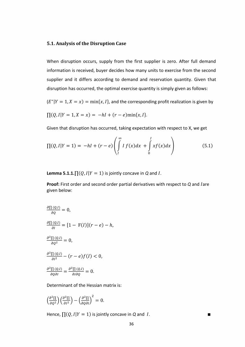
5.1. Analysis of the Disruption Case

When disruption occurs, supply from the first supplier is zero. After full demand

information is received, buyer decides how many units to exercise from the second

supplier and it differs according to demand and reservation quantity. Given that

disruption has occurred, the optimal exercise quantity is simply given as follows:

( | { }, and the corresponding profit realization is given by

| { }.

Given that disruption has occurred, taking expectation with respect to X, we get

| (∫

∫

)


Proof: First order and second order partial derivatives with respect to Q and are given below:

[ ] ,

,

Determinant of the Hessian matrix is:

(

) (

) (

)


37

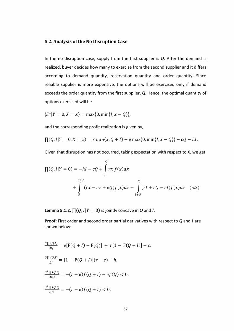
5.2. Analysis of the No Disruption Case

In the no disruption case, supply from the first supplier is Q. After the demand is

realized, buyer decides how many to exercise from the second supplier and it differs

according to demand quantity, reservation quantity and order quantity. Since

reliable supplier is more expensive, the options will be exercised only if demand

exceeds the order quantity from the first supplier, Q. Hence, the optimal quantity of

options exercised will be

( | { { }},

and the corresponding profit realization is given by,

| { } { { }} .

Given that disruption has not occurred, taking expectation with respect to X, we get

| ∫

∫ ∫


Proof: First order and second order partial derivatives with respect to Q and are shown below:

[ ] [ ]

[ ] ,

,

,

38

= .

Determinant of the Hessian matrix is given as follows:

(

) (

) (

)


5.3. Analysis of the Full Information Model

In this section, we formulate and analyze the full information model by combining

the results of Section 5.1 and Section 5.2.Utilizing Equation (5.1) and Equation (5.2),

and taking expectation with respect to Y, the expected profit of the buyer can be

characterized as

[∫

∫

]

[∫

∫

∫

]


Max

Subject to ,


(reliable) supplier. Then, the following theorem characterizes the optimal solution

to the buyer’s problem.

39

Theorem 5.3.1. If

, then and (

). Otherwise, we

have and given by the unique solution to

= 0 and

= 0.

Proof: Since the objective function is strictly concave and the constraints are linear,

there exists a unique optimal solution to the buyer’s problem which can be

characterized by the following KKT conditions:

[ ] (5.3)

[ ] (5.4)

(5.5)

(5.6)

(5.7)

We next analyze four possible cases (i) (ii) (iii)

(iv) .

(i) When , we have and from Equation (5.5) and

Equation (5.6), respectively. Then, Equation (5.3) reduces to

, which violates the nonnegativity condition. Hence,

cannot be optimal.

(ii) When we have and from Equation (5.5) and

Equation (5.6), respectively. Then, from Equation (5.3), we get

. Plugging it into Equation (5.4), we obtain

[ ] , which violates the nonnegativity condition. Hence,

cannot be optimal.

(iii) When , we have and from Equation (5.5) and

Equation (5.6), respectively. Then, Equation (5.4) reduces to

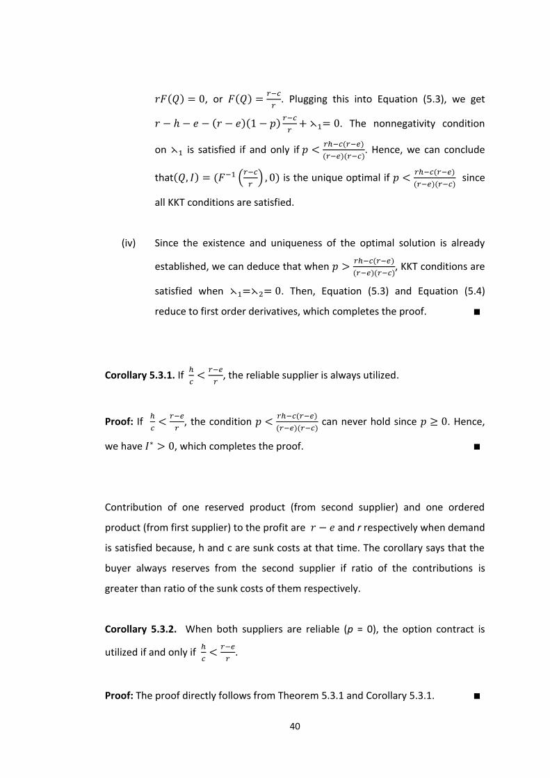
40

, or

. Plugging this into Equation (5.3), we get

. The nonnegativity condition

on is satisfied if and only if

. Hence, we can conclude

that (

) is the unique optimal if

since

all KKT conditions are satisfied.

(iv) Since the existence and uniqueness of the optimal solution is already

established, we can deduce that when

, KKT conditions are

satisfied when . Then, Equation (5.3) and Equation (5.4)

reduce to first order derivatives, which completes the proof.

Corollary 5.3.1. If

, the reliable supplier is always utilized.

Proof: If

, the condition

can never hold since . Hence,

we have , which completes the proof.

Contribution of one reserved product (from second supplier) and one ordered

product (from first supplier) to the profit are and r respectively when demand

is satisfied because, h and c are sunk costs at that time. The corollary says that the

buyer always reserves from the second supplier if ratio of the contributions is

greater than ratio of the sunk costs of them respectively.

Corollary 5.3.2. When both suppliers are reliable (p = 0), the option contract is

utilized if and only if

.

Proof: The proof directly follows from Theorem 5.3.1 and Corollary 5.3.1.

41

When the first supplier is reliable like the second supplier, buyer uses the second

supplier if and only if contribution of one reserved product from the second

supplier to the profit is greater than one ordered product from the first supplier.

Since the solution is trivial when

, we continue our analysis for the

cases with

, where the optimal solution is given by the first order

conditions.

Corollary 5.3.3. ( ) is non-increasing (non-decreasing) in the disruption

probability, p

Proof: Let and denote

and

respectively. From

we have

(5.8)

Then from the implicit derivative of

with respect to p, we have

+ . Hence and have opposite signs. Plugging

(5.8) into

, we get ( )

.Taking the implicit derivative with respect to p, we have

, which

can be written as [ ]

noting that we have from Equation (5.8). In

order for the last equality to hold, we need to have and , which

completes the proof.

This corollary can be interpreted as follows: when the disruption probability

increases, buyer reserves more from the second supplier which is quite intuitive

because the possibility of meeting demand only from the second supplier is

increased. Also, buyer should not increase its order from the first supplier because if

it is increased and the first supplier does not face disruption, the buyer has to take

42

all of the supply from the first supplier so cost of increased reserved quantity

becomes a loss.

Corollary 5.3.4. ( ) is non-decreasing (non-increasing) in cost of per unit

reserved from the second supplier, h.


Appendix A.

The buyer decreases its reservation quantity as the cost of per unit reserved from

the second supplier increases when all other problem parameters are the same. In

the case of decreased reservation quantity, buyer should increase order quantity

from the first supplier in order to compensate it in a no disruption case.

Corollary 5.3.5. ( ) is non-increasing (non-decreasing) in cost of per unit from

the first supplier, c.


Appendix B.

The buyer decreases its order as the cost of per unit ordered from the first supplier

increases when all other problem parameters are the same. Loss due to unmet

demand in a no disruption case because of the inadequacy of supply is less when

cost of per unit ordered from the first supplier increases. Hence, buyer accepts this

loss risk by decreasing order. In the case of decreased order quantity, buyer should

increase reservation quantity from the second supplier in order to compensate it in

each case, disruption and no disruption.

Corollary 5.3.6. ( ) is non-decreasing (non-increasing) in cost of per unit

exercised from the second supplier, e.

43


Appendix C.

The buyer decreases its optimal reservation quantity as the cost of per unit

exercised from the second supplier increases when all other problem parameters

are the same. In this case the buyer should increase order quantity from the first

supplier in order to compensate it in a no disruption case.

Corollary 5.3.7. is non-decreasing in the revenue per unit, r.


Appendix D.

This corollary can be interpreted as follows: the buyer wants to increase reservation

quantity as the revenue per unit increases. He earns more profit from one product

sale if it is satisfied from reserved quantity. Although increasing reservation

quantity increases the risk that more reserved quantity will be wasted when

demand is satisfied from the first supplier, buyer increases reservation quantity as

the revenue per unit increases. We expect is non-decreasing in the revenue but

we cannot show analytically. Because when the revenue increases the buyer earns

more profit from one product sale if it is satisfied from the first supplier’s supply.

The summary of all analytical solution that we derived is depicted in Table 5.1.

44

45

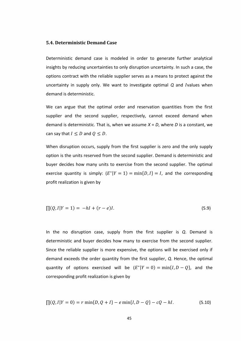
5.4. Deterministic Demand Case

Deterministic demand case is modeled in order to generate further analytical

insights by reducing uncertainties to only disruption uncertainty. In such a case, the

options contract with the reliable supplier serves as a means to protect against the

uncertainty in supply only. We want to investigate optimal Q and values when

demand is deterministic.

We can argue that the optimal order and reservation quantities from the first

supplier and the second supplier, respectively, cannot exceed demand when

demand is deterministic. That is, when we assume X = D, where D is a constant, we

can say that and .

When disruption occurs, supply from the first supplier is zero and the only supply

option is the units reserved from the second supplier. Demand is deterministic and

buyer decides how many units to exercise from the second supplier. The optimal

exercise quantity is simply: ( | { } , and the corresponding

profit realization is given by

| . (5.9)

In the no disruption case, supply from the first supplier is Q. Demand is

deterministic and buyer decides how many to exercise from the second supplier.

Since the reliable supplier is more expensive, the options will be exercised only if

demand exceeds the order quantity from the first supplier, Q. Hence, the optimal

quantity of options exercised will be ( | { }, and the

corresponding profit realization is given by

| { } { } . (5.10)

46

Utilizing Equation (5.12) and Equation (5.13), and taking expectation with respect to

Y, the expected profit of the buyer can be characterized as

[ { } { } ]

{

(5.11)


Max

Subject to


(reliable) supplier.

Lemma 5.4.1.For a given Q, if , then . Otherwise

.

Proof: Taking the derivative of the profit function with respect to , we get

= {

. (5.12)

If , from Equation (5.12) we can argue that the profit function is

non-decreasing in because the derivative is nonnegative in either region,(

and ). Hence, we have since D is the upper bound on .

If , from Equation (5.12) we can argue that the profit function

increases as the reservation quantity ( ) increases until because the

derivative is in this region ( ). For , the profit

47

function decreases as the reservation quantity ( ) increases because the derivative

is To sum up, the expected profit increases in until

and decreases in afterwards. Hence, the optimal reservation quantity occurs at

the breakpoint, .

Lemma 5.4.2.For a given , if , then . Otherwise .

Proof: Taking the derivative of the profit function with respect to , we get

= {

. (5.13)

If , from Equation (5.13) we can argue that the profit function increases as the

order quantity (Q) increases because the derivative is always positive. Since Q can

be at most D, we have .

If , from Equation (5.13) we can argue that the profit function increases as the

order quantity (Q) increases until because the derivative is

,in this region . For , the profit function decreases as the

order quantity (Q) increases because the derivative, . To sum up,

the profit function increases in until and decreases in afterwards.

Hence, the optimal order quantity occurs at the breakpoint, .

Our findings in Lemma 5.4.1 and Lemma 5.4.2 can be summarized as follows:

(i) If and , .

(ii) If and , .

(iii) If and , .

(iv) If and , .

The optimal solutions are already found in cases (i), (ii), (iii). We next analyze case

(iv) in detail because we only know for this case.

48

Lemma 5.4.3.Given that and , if

then , otherwise .

Proof: Plugging into (5.11), the expected profit function reduces to

. (5.14)

Taking the derivative of (5.14) with respect to , we get

. (5.15)

If , from (5.15) we can argue that the profit

function increases as the reservation quantity ( ) increases because the derivative is

positive. Hence, .

If , from (5.15) we can argue that the profit

function decreases as the reservation quantity ( ) increases because the derivative

is negative. Hence, , which completes the proof.

49

Theorem 5.4.3.Under deterministic demand, the optimal order and reservation

quantities are

Table 5.2 Optimal Values with Deterministic Demand

Conditions

(i) - D D

(ii) - 0 D

(iii) - D 0

(iv)

0 D

0 D 0

Proof: The optimal solutions and their conditions can be seen directly from Lemma

5.4.1, 5.4.2 and Lemma 5.4.3.

This theorem gives insights about buyer’s order and reservation quantity decisions.

Demand is deterministic so the buyer makes these decisions according to cost and

revenue parameters and disruption uncertainty. Since the only uncertainty is

disruption and uncertainty in disruption is discrete, buyer makes orders or

reservation as zero or demand quantity.


is when , otherwise it is .

Buyer earns for one exercised unit in disruption case because there is no

opportunity other than using second supplier, in no disruption case because

there is an opportunity to supply from the first supplier so opportunity cost of using

50

second supplier rather than first supplier, .We take expectation according to Y

and the expected profit becomes . However, in no

disruption case buyer always uses first supplier when because he doesn’t

want to give more money when he has an opportunity to supply from the first

supplier. Hence, expected profit per unit is when .


{

If this profit is positive in either case, buyer always makes reservation as demand

quantity. Otherwise, he reserves nothing.

Buyer makes order decision according to the purchasing cost difference between

two suppliers and expected profit per unit if the buyer uses second supplier rather

than first supplier. If the cost difference, , is negative, buyer always makes an

order as demand quantity. Buyer can also order as demand quantity when , is

positive and the expected profit per unit if the buyer uses second supplier rather

than first supplier is negative, he orders as demand quantity.

Corollary 5.3.1. When

, and (

) whatever the

information level is about demand and disruption uncertainty.

Proof: In the full information model, Theorem 5.3.1 shows that when

,

then and (

). In the partial information model, Corollary 4.2.1

shows that when and then and (

)and

when and then and

(

). In the no information model, Theorem 5.3.1 shows that when

, then and (

). The

condition

in the full information model can be written as

51

[ ]

and it is equivalent to [

] . When this inequality holds, .For , we have

as well, and the corollary follows. For

,[ ] [ ].

So, we conclude that if

, [ ]

and always hold. Hence, buyer never use second supplier

whatever the information level is when


Corollary 5.3.2.When or , disruption

information is completely worthless.

Proof: From theorem 5.3.1 and corollary 4.3.1,if , optimal and values are

the same in partial and no information models in the same conditions. That is, when

, we have the trivial solution we have

(

) and ; otherwise we have (

) and .

We next consider and . From Theorem 5.3.1 and Corollary

4.3.1, we have (

) and in both models, which completes the

proof.

This corollary demonstrates us disruption information is worthless not only in the

trivial case , but also in some cases that buyer uses options contract.

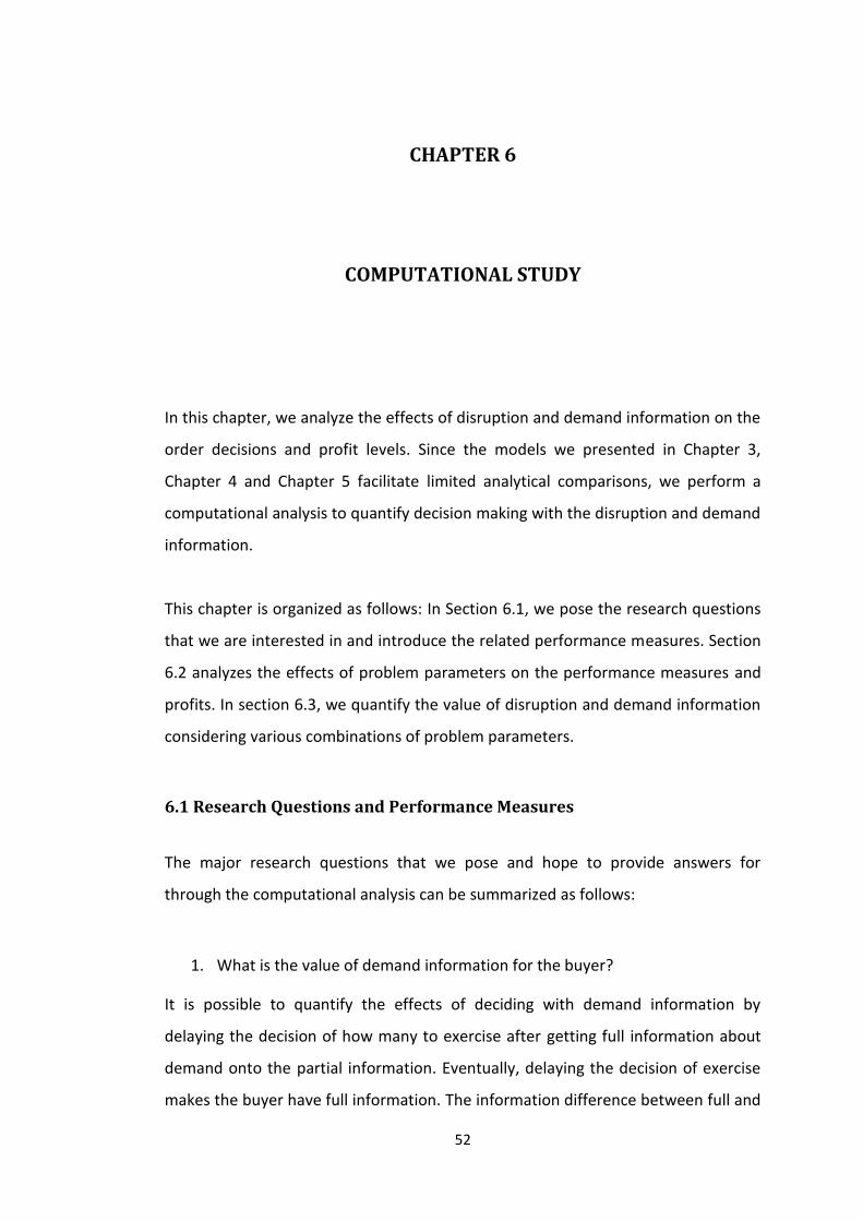
52

CHAPTER 6

COMPUTATIONAL STUDY

In this chapter, we analyze the effects of disruption and demand information on the

order decisions and profit levels. Since the models we presented in Chapter 3,

Chapter 4 and Chapter 5 facilitate limited analytical comparisons, we perform a

computational analysis to quantify decision making with the disruption and demand

information.

This chapter is organized as follows: In Section 6.1, we pose the research questions

that we are interested in and introduce the related performance measures. Section

6.2 analyzes the effects of problem parameters on the performance measures and

profits. In section 6.3, we quantify the value of disruption and demand information

considering various combinations of problem parameters.

6.1 Research Questions and Performance Measures

The major research questions that we pose and hope to provide answers for

through the computational analysis can be summarized as follows:

1. What is the value of demand information for the buyer?

It is possible to quantify the effects of deciding with demand information by

delaying the decision of how many to exercise after getting full information about

demand onto the partial information. Eventually, delaying the decision of exercise

makes the buyer have full information. The information difference between full and

53

partial information model is deciding how many to exercise from the second

supplier with demand information.

2. What is the value of disruption information for the buyer?

In partial information, disruption uncertainty is resolved prior to exercise decision

by means of the options contract. If there is no chance to sign an options contract,

buyer has to make the decision of order from the second supplier when all

uncertainties exist. Eventually, nonexistence of options contract makes the buyer

have no information. The information that the buyer knows is disruption in the

partial information model.

In seeking answers to the above questions, we start with a sensitivity analysis to

characterize how the performance measures mentioned below are affected by the

changes in problem parameters in Section 6.2. Then we perform a full factorial

design in Section 6.3 to analyze the results with a number of different parameter

sets. Performance measures include the percentage improvement in expected

profits due to disruption and demand information. More specifically performance

measures are;

For question 1, we compare full information with partial information and

calculate % profit improvement due to full information over partial

information. It is the value of demand information. We define the

performance measure as follows: (

) for the buyer’s

profit.

For question 2, we compare partial information with no information and

calculate % profit improvement due to partial information over no

information. It is the value of disruption information. We define the

54

performance measure as follows: (

) for the buyer’s

profit.

6.2 Analysis of Parameter Sensitivity

Sensitivity analysis is conducted for the parameters used in the models according to

the base parameter set defined. Performance measures are evaluated while each

parameter is increased and others kept as in the base parameter set. Base

parameter set is selected in such a way that the condition in Corollary 5.3.1 doesn’t

hold. In other words, under the base parameter setting, optimal order and

reservation decisions are non-zero. The base parameter set used in the sensitivity

analysis is provided in Table 6.1.

Table 6.1: Base parameter set values.

150 30 24 5 0.1 10 100

6.2.1 Disruption Probability

We start with the analysis of disruption probability. Recall that uncertainty in supply

disruption is discrete, first supplier disrupts according to the random variable, Y.

When with the probability , then supply from the first supplier is ,

otherwise supply is . Overall results for problem instances considered are

provided in Table G.1 in Appendix G. is changed between 0.01 and 0.9 with a step

size of 0.05. We present our observations with respect to an increase in :

In the optimal solutions of all models, buyer’s profit shows a decreasing

behavior in a manner that in full and partial information it experiences a

steep decrease until , in no information until and after

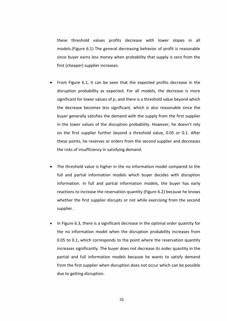
55

these threshold values profits decrease with lower slopes in all

models.(Figure 6.1) The general decreasing behavior of profit is reasonable

since buyer earns less money when probability that supply is zero from the

first (cheaper) supplier increases.

From Figure 6.1, it can be seen that the expected profits decrease in the

disruption probability as expected. For all models, the decrease is more

significant for lower values of , and there is a threshold value beyond which

the decrease becomes less significant, which is also reasonable since the

buyer generally satisfies the demand with the supply from the first supplier

in the lower values of the disruption probability. However, he doesn’t rely

on the first supplier further beyond a threshold value, 0.05 or 0.1. After

these points, he reserves or orders from the second supplier and decreases

the risks of insufficiency in satisfying demand.

The threshold value is higher in the no information model compared to the

full and partial information models which buyer decides with disruption

information. In full and partial information models, the buyer has early

reactions to increase the reservation quantity (Figure 6.2) because he knows

whether the first supplier disrupts or not while exercising from the second

supplier.

In Figure 6.3, there is a significant decrease in the optimal order quantity for

the no information model when the disruption probability increases from

0.05 to 0.1, which corresponds to the point where the reservation quantity

increases significantly. The buyer does not decrease its order quantity in the

partial and full information models because he wants to satisfy demand

from the first supplier when disruption does not occur which can be possible

due to getting disruption.

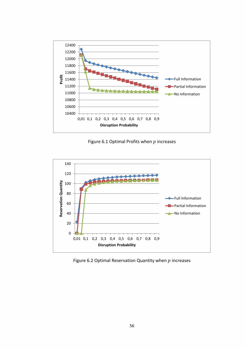
56

Figure 6.1 Optimal Profits when increases

Figure 6.2 Optimal Reservation Quantity when increases

10400

10600

10800

11000

11200

11400

11600

11800

12000

12200

12400

0,01 0,1 0,2 0,3 0,4 0,5 0,6 0,7 0,8 0,9

Pro

fit

Disruption Probability

Full Information

Partial Information

No Information

0

20

40

60

80

100

120

140

0,01 0,1 0,2 0,3 0,4 0,5 0,6 0,7 0,8 0,9

Re

serv

atio

n Q

uan

tity


Full Information

Partial Information

No Information

57

Figure 6.3 Optimal Order Quantity when increases

Figure 6.4 shows the percentage profit improvement due to full information

over partial information (FoP) and due to partial information over no

information (PoN). PoN increases until and decreases afterwards. It

is the point where the buyer begins to increase its reservation quantity also

in the no information model and decrease the risk of stock-out in satisfying

demand.

FoP shows an increasing behavior since exercising after getting demand

information decreases the number of units that is exercised for nothing in

the full information model.

0

20

40

60

80

100

120

0,01 0,1 0,2 0,3 0,4 0,5 0,6 0,7 0,8 0,9

Ord

er

Qu

anti

ty


Full Information

Partial Information

No Information

58

Figure 6.4 PoN and FoP when increases

6.2.2 Standard Deviation of Demand

We analyze the sensitivity of our results to the standard deviation of the Normal

random variable, . Overall results for the problem instances considered are

provided in Table G.2 in Appendix G. is changed between 5 and 30 with a step

size of 5. We present our observations with respect to an increase in :

In the optimal solutions of all models, buyer’s profit shows a decreasing

behavior in standard deviation as expected. In Figure 6.5, we observe

that the decrease in the partial and no information models is steeper

than it is in the full information model. Since the buyer doesn’t have

demand information while exercising under these cases, his profit is

dampened more when demand uncertainty increases.

The value of demand information increases as the standard deviation of

demand increases. As we expected, the value of demand information,

that is FoP, increases in Figure 6.6. There is no significant difference in

the percentage profit improvement when we compare partial and no

0

0,5

1

1,5

2

2,5

3

3,5

4

4,5

5

0,01 0,1 0,2 0,3 0,4 0,5 0,6 0,7 0,8 0,9

Pe

rce

nta

ge Im

pro

vem

en

t


PoN

FoP

59

information models (PoN). It is reasonable because in either case the

demand uncertainty is not resolved.


Figure 6.6 Performance Measures when increases

From Figures 6.7 and 6.8, we can see that the buyer prefers to order more

from the second supplier and less from the first supplier as increases in

9500

10000

10500

11000

11500

12000

12500

5 10 15 20 25 30

Pro

fit

Standard Deviation

Full Information

Partial Information

No Information

0

1

2

3

4

5

6

7

8

5 10 15 20 25 30

Pe

rce

nta

ge Im

pro

vem

en

t

Standard Deviation

PoN

FoP

60

the full information model. However, in the partial and no information

models, he prefers to order more from the first supplier.

Figure 6.7 Optimal Reservation quantity when increases

Figure 6.8 Optimal Order quantity when increases

0

20

40

60

80

100

120

5 10 15 20 25 30

Re

serv

atio

n Q

uan

tity

Standart Deviation

Full Information

Partial Information

No Information

0

20

40

60

80

100

120

140

5 10 15 20 25 30

Ord

er

Qu

anti

ty

Standard Deviation

Full Information

Partial Information

No Information

61

6.2.3 Unit Cost of the First Supplier

We analyze the sensitivity of our results to the unit cost of the first supplier, .

Overall results for problem instances considered are provided in Table G.3 in

Appendix G. is changed between 22 and 32 with a step size of 1. We present our

observations with respect to an increase in :

The optimal profit decreases as the unit cost increases until a threshold

value after which the profits stay almost the same. We can see from Figure

6.9 that the profit under partial information decreases with the greatest

slope and the profit under no information decreases with the least slope.


FoP increases PoN decreases. As the profit margin when demand is satisfied

from the first supplier decreases as the unit cost increases. The buyer orders

less from the first supplier and orders more from the second supplier in the

no information model (Figure 6.12) because the cost difference between

suppliers decreases. In the same way, the buyer reserves as much as

demand plus standard deviation (Figure 6.11) and having a chance to

exercise after getting disruption information is now less important the in

partial information model. Therefore, we can see from Figure 6.10 that the

10400

10600

10800

11000

11200

11400

11600

11800

12000

12200

22 23 24 25 26 27 28 29 30 31 32

Pro

fit

Unit Cost

Full Information

Partial Information

No Information

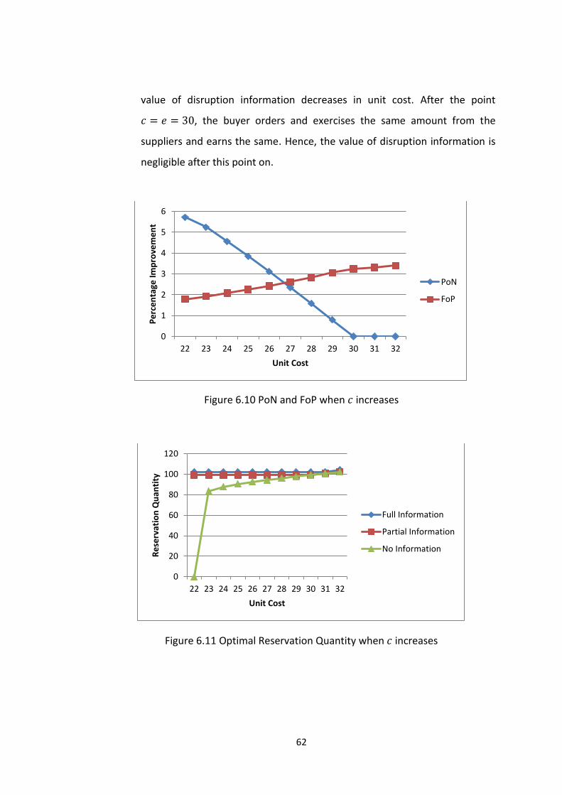
62

value of disruption information decreases in unit cost. After the point

, the buyer orders and exercises the same amount from the

suppliers and earns the same. Hence, the value of disruption information is

negligible after this point on.



0

1

2

3

4

5

6

22 23 24 25 26 27 28 29 30 31 32

Pe

rce

nta

ge Im

pro

vem

en

t

Unit Cost

PoN

FoP

0

20

40

60

80

100

120

22 23 24 25 26 27 28 29 30 31 32

Re

serv

atio

n Q

uan

tity

Unit Cost

Full Information

Partial Information

No Information

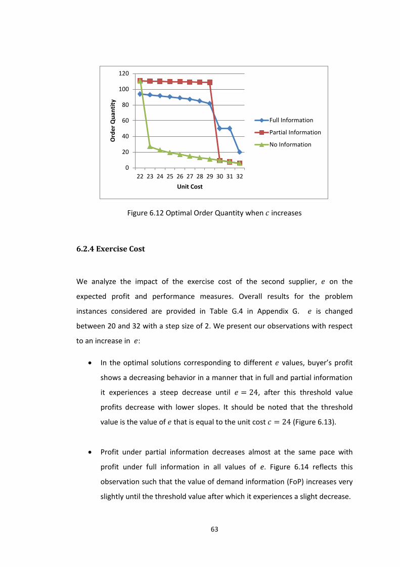
63


6.2.4 Exercise Cost

We analyze the impact of the exercise cost of the second supplier, on the

expected profit and performance measures. Overall results for the problem

instances considered are provided in Table G.4 in Appendix G. is changed

between 20 and 32 with a step size of 2. We present our observations with respect

to an increase in :

In the optimal solutions corresponding to different values, buyer’s profit

shows a decreasing behavior in a manner that in full and partial information

it experiences a steep decrease until , after this threshold value

profits decrease with lower slopes. It should be noted that the threshold

value is the value of that is equal to the unit cost (Figure 6.13).

Profit under partial information decreases almost at the same pace with

profit under full information in all values of e. Figure 6.14 reflects this

observation such that the value of demand information (FoP) increases very

slightly until the threshold value after which it experiences a slight decrease.

0

20

40

60

80

100

120

22 23 24 25 26 27 28 29 30 31 32

Ord

er

Qu

anti

ty

Unit Cost

Full Information

Partial Information

No Information

64

In the no information case, profit decreases almost with the same slope

which is always greater than it is in the partial information case (Figure

6.13). Before the point , buyer orders and exercises the same

amount from the suppliers and earns the same so disruption information is

negligible before this point. The profit margin when demand is satisfied from

the first supplier increases comparatively as the exercise cost increases. As

observed in Figure 6.16, the buyer orders more from the first supplier and

orders less from the second supplier in the no information model. In the

same way, buyer orders as much as demand plus standard deviation (Figure

6.15) and having a chance to exercise after getting disruption information is

more important in the partial information model. Therefore, we can see

from Figure 6.14 that value of disruption information (PoN) increases in the

exercise cost.


10000

10500

11000

11500

12000

12500

20 22 24 26 28 30 32

Pro

fit

Exercise Cost

Full Information

Partial Information

No Information

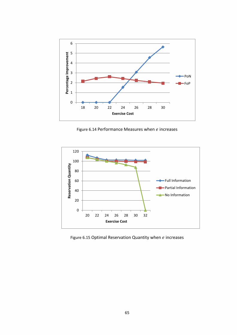
65



0

1

2

3

4

5

6

18 20 22 24 26 28 30

Pe

rce

nta

ge Im

pro

vem

en

t

Exercise Cost

PoN

FoP

0

20

40

60

80

100

120

20 22 24 26 28 30 32

Re

serv

atio

n Q

uan

tity

Exercise Cost

Full Information

Partial Information

No Information

66


6.2.5 Revenue

We analyze the impact of the revenue per unit, on optimal profit and

performance measures. Overall results for problem instances considered are

provided in Appendix G. is changed between 100 and 200 with a step size of 25.

We present our observations with respect to an increase in :

When revenue increases, ratio of profit of one unit over cost of one unit

increases exponentially. In such a case, buyer wants to reduce the risk of

stock-out more since having a stock-out is now more costly. In full and

partial information models, he orders and reserves about mean demand. In

the no information model, he orders more from the second supplier and less

from the first supplier (Figure 6.20). This makes deciding with disruption and

demand information less important and in Figure 6.18, we can see the

decrease in the value of disruption and demand information. There is an

increase in the value of disruption information from to

because buyer reserves nothing in these points. (Figure 6.19)

0

20

40

60

80

100

120

20 22 24 26 28 30 32

Ord

er

Qu

anti

ty

Exercise Cost

Full Information

Partial Information

No Information

67



5000

7000

9000

11000

13000

15000

17000

19000

100 125 150 175 200

Pro

fit

Revenue

Full Information

Partial Information

No Information

0

0,5

1

1,5

2

2,5

3

3,5

4

4,5

5

100 125 150 175 200

Pe

rce

nta

ge Im

pro

vem

en

t

Revenue

PoN

FoP

68



6.2.6 Reservation Cost

We analyze the impact of the reservation cost per unit, on the expected profit and

performance measures. Overall results for the problem instances considered are

provided in Appendix G. is changed between 1 and 33 with a step size of 4. We

present our observations with respect to an increase in :

0

20

40

60

80

100

120

100 125 150 175 200

Re

serv

atio

n Q

uan

tity

Revenue

Full Information

Partial Information

No Information

0

20

40

60

80

100

120

100 125 150 175 200

Ord

er

Qu

anti

ty

Revenue

Full Information

Partial Information

No Information

69

In Figure 6.21, we can see that profits are getting closer to each other. After

the point , profits are the same and the values of disruption and

demand information are negligible because the buyer doesn’t use options

contract in any information level (Figure 6.23).

In Figure 6.22, PoN and FoP values decrease as the reservation cost

increases and after the point they are the same. After this point,

options contract is very costly to use, the buyer ignores the second supplier

and use the first supplier in any model so profits, PoN, FoN and order

quantities are the same.

Figure 6.21 Profit when increases

10000

10500

11000

11500

12000

12500

1 5 9 13 17 21 25 29 33

Pro

fit

Reservation Cost

Full Information

Partial Information

No Information

70



-1

0

1

2

3

4

5

1 5 9 13 17 21 25 29 33

Pe

rce

nta

ge Im

pro

vem

en

t

Reservation Cost

PoN

FoP

0

20

40

60

80

100

120

1 5 9 13 17 21 25 29 33

Re

serv

atio

n Q

uan

tity

Reservation Cost

Full Information

Partial Information

No Information

71


6.3 Analysis of Full Factorial Design

A full factorial experiment is designed for the parameter values given in Table 6.2.

The aim of the full factorial experiment is to detect the value of disruption and

demand information. All combinations of these parameter values (totally 4096

problem instances) are solved for all models to analyze the results for defined

research questions in Section 6.1.

Table 6.2: Parameters values used for full factorial design

100 125 150 175

24 27 30 33

10 16 22 28

5 8

10 12

0.01 0.05 0.1

0.25

10 20 25

33.3

100

0

20

40

60

80

100

120

1 5 9 13 17 21 25 29 33

Ord

er

Qu

anti

ty

Reservation Cost

Full Information

Partial Information

No Information

72

6.3.1 Value of Disruption Information

In partial information model, disruption uncertainty is resolved prior to the exercise

decision by means of the options contract. If there is no chance to sign an options

contract, buyer has to order from the second supplier when all uncertainties still

exist. In partial information, buyer makes the decision of how many to exercise

from the second supplier after observing the disruption or lack of it. Hence, we can

quantify the value of disruption information by computing % profit improvement on

partial information model’s profit over no information model’s profit. Average

values are found over all 4096 numerical combinations.

OBSERVATION 1. Optimal profit in the partial information model is always greater

than or equal to the optimal profit in the no information model. The maximum,

minimum and average values of PoN over all problem instances are provided in

Table 6.3. Deciding how many to exercise from the second supplier with disruption

information improves buyer’s profit with 18.9% maximum and 2.1% on average in

our 4096 numerical combinations. The maximum value is found at a point such that

disruption probability and cost difference between ordering from the first supplier

and exercising from the second supplier are the highest in the parameter

values of full factorial design. This coincides with the findings in sensitivity analysis

part.

73

Table 6.3 Percentage improvements on profit under partial information over profit

under no information

MAX MIN AVG

% system profit improvement on PI over NI,(

) 18.9% 0% 2.1%

125 100 -

10 28 -

33 27 -

5 5 -

0.25 0.25 -

10 33.3 -

OBSERVATION 2. Disruption probability, , is one of the most important parameters

that change the value of disruption information. Table 6.4 shows disruption

information is highly valuable for high values of disruption probability. Maximum

and average profit improvements decrease as disruption probability decreases.

OBSERVATION 3. Profits of partial and no information is the same when so

disruption information is negligible.

Table 6.4 PoN values for different values.

max 18.9% 6.4% 1.5% 0.0%

min 0.0% 0.0% 0.0% 0.0%

avg 6.8% 1.4% 0.1% 0.0%

74

OBSERVATION 4. Difference between exercise cost and unit cost , is another

important parameter that changes the value of information significantly. Table 6.5

shows disruption information is highly valuable for high values of, . Maximum

and average profit improvements decrease as the cost difference decreases.

OBSERVATION 5. We can directly conclude that when , from Table 6.5,

profits of partial and no information are the same so disruption information is

negligible. This is also proved in Corollary 5.3.2 so that optimal order and

reservation quantities are equal. We have also found the point, as a threshold

value from the figures of sensitivity analysis. Here we prove this point is a critical

value about profit improvements.


max 18.9% 6.4% 2.7% 0.0%

min 0.0% 0.0% 0.0% 0.0%

avg 3.6% 2.6% 0.7% 0.0%

OBSERVATION 6. Difference between unit cost and reservation cost , is

another important parameter that changes the value of disruption information

significantly. Table 6.6 shows disruption information is highly valuable for low

values of, . Maximum and average profit improvements increase as the

difference decreases.


max 6.7% 13.1% 14.5% 15.2%

min 0.0% 0.0% 0.0% 0.0%

avg 0.8% 1.8% 2.4% 2.5%

75

OBSERVATION 7. Reservation cost and standard deviation of demand do not change

the value of disruption information significantly. On the other hand, increase in

revenue decreases average profit improvement significantly.

Figure 6.12 shows how increase in reservation cost, revenue and standard deviation

affect the average profit improvement. Parameter values are increasing from first to

fourth value according to full factorial design.

Figure 6.25 Average Profit Improvements according to Problem Parameters

OBSERVATION 8. Reservation quantity in the partial information model is always

greater than or equal to the reservation quantity under no information for all

parameter combinations of factorial design.

0

1

2

3

4

5

6

7

8

FirstValue

SecondValue

ThirdValue

FourthValue

Ave

rage

Po

N

Revenue

Standard Deviation

Reservation Cost

76

6.3.2 Value of Demand Information

In the full information model, exercise decision is delayed after getting information

about demand. In partial information model, there is an uncertainty of demand

while exercising from the second supplier. Hence, we can quantify the value of

demand information by computing % profit improvement due to full information

over partial information.

OBSERVATION 9. Optimal profit under full information is always greater than or

equal to the optimal profit under partial information. The maximum, minimum and

average values of FoP over all problem instances are provided in Table 6.7. Deciding

how many options to exercise from the second supplier with demand information

improves buyer’s profit with 16.2% maximum and 3.1% on average in our 4096

numerical combinations. The maximum value is found at a point such that standard

deviation is the highest and difference revenue and unit cost is the lowest in

the parameter values of full factorial design. This coincides with the findings in

sensitivity analysis part.

Table 6.7 Percentage improvements on profit under full information over profit

under partial information

MAX MIN AVG

% system profit improvement on FI over PI, (

) 16.2% 0% 3.1%

100 100 -

28 16 -

27 33 -

5 12 -

0.25 0.01 -

1110 1110 -

77

OBSERVATION 10. Standard deviation of demand, , is highly significant in the value

of demand information. Buyer can increase his profit by 16.2% maximum and 3.1%

in average in 4096 instances if he decides the exercise quantity with demand

information. Table 6.8 shows demand information is more valuable for high values

of the standard deviation. Maximum and average profit improvements increase as

the standard deviation increases.

Table 6.8 FoP values for different values.

max 16.2% 11.9% 9.4% 4.4%

min 0.0% 0.0% 0.0% 0.0%

avg 4.8% 3.5% 2.8% 1.3%

OBSERVATION 11. Difference between revenue and unit cost, , significantly

impacts the value of demand information. Table 6.8 shows demand information is

more valuable for low values of, . Maximum and average profit improvements

value decreases as the difference between revenue and unit cost increases.


max 2.9% 8.6% 13.1% 16.2%

min 0.0% 0.2% 0.6% 0.5%

avg 1.0% 3.5% 5.9% 6.6%

OBSERVATION 12. Difference between unit cost and reservation cost , is

another important parameter that changes the value of demand information

significantly. Table 6.10 shows demand information is highly valuable for high

values of, . Maximum and average profit improvements decrease as the

difference decreases.

78


max 16.2% 12.2% 7.1% 3.7%

min 1.7% 0.5% 0.02% 0.0%

avg 6.8% 3.9% 1.8% 0.7%

OBSERVATION 13. Reservation and exercise cost do not have a significant effect on

the value of demand information whereas an increase in disruption probability

increases the average profit improvement significantly.

Figure 6.26 Average Profit Improvements according to Problem Parameters

OBSERVATION 14. Reservation quantity under full information is always greater

than or equal to the reservation quantity under partial information for all

parameter combinations.

0

0,5

1

1,5

2

2,5

3

3,5

4

4,5

5

1 2 3 4

Ave

rage

Fo

P

Parameter Values

Exercise Cost


Reservation Cost

79

CHAPTER 7

CONCLUSION

Supply disruption literature has been growing quickly in the past few years,

motivated by increased globalization. Firms now choose suppliers from anywhere in

the world because of increased price sensitivity of markets. Events like natural

disasters (earthquake, fire etc.), terrorist attacks, war, strike etc. happening in

another country or continent can affect your deliveries very seriously. Supply goes

off totally in these circumstances so firms should mitigate the disruption risk. This is

why supply disruption is an emerging interest area in the past years.

In this study, we consider a single-period problem with a buyer that faces random

demand. The buyer has two alternative suppliers: one cheaper but prone to

disruption and the other perfectly reliable but more expensive. The models

presented here are designed to show (i) how the buyer orders from the two

suppliers, (ii) in which cases options contract is used, (iii) what are the managerial

benefits of higher information levels about disruption and demand risk bring.

We developed efficient approaches to quantify the value of two important supply

risk mitigation strategy in a dual sourcing supply chain with options contract: (1)

obtaining disruption risk information, and (2) obtaining demand risk information

before using options. We defined measures for the value of obtaining disruption as

well as the value of obtaining demand risk information. These measures are the

upper bounds for the amount of money that a risk-neutral firm should be willing to

80

invest to implement either of these strategies in order to mitigate uncertainties in

its supply chain system.

In all information levels, we analytically characterized the buyer's behavior by

explicitly identifying the optimal size of order and reservation according to all cost,

revenue and uncertainty parameters. We demonstrated the circumstances that the

buyer uses options contract and found closed form solutions about order and

reservation quantities when options contract is used. We defined performance

measures and showed analytically and theoretically how problem parameters

influence these measures, profits and quantities. A computational study is

conducted and our analyses reveal the following findings:

Delaying the decision of how many to exercise from the second supplier

provides greater profits due to having information about disruption and

demand uncertainties.

If the buyer doesn’t use options contract in an information level, it is also

not used in the lower information levels.

In any information level, buyer makes more reservation than he makes in

lower information levels in the same values of parameters.

When the buyer doesn’t use options contract, he orders the same amount

from the first supplier in any information level.

Increase in disruption probability increases value of disruption risk

information and increase in variability of demand increases value of demand

risk information.

One of the main results of Chopra (2007) says that “Growth in supply risk from

increased disruption probability is best mitigated by increased use of the reliable

(though more expensive) supplier and decreased use of the cheaper but less

reliable supplier.” This coincides with our results such that reservation quantity is

non-decreasing and order quantity is non-increasing in disruption probability in any

information level. In one of the observations in Saghafian and Van Oyen (2011), it is

81

found that disruption risk information is more valuable to firms with lower profit

margins. This is parallel to our observations in computational study; we observe

that changing revenue and cost parameters so that the profit margin decreases

makes disruption information more attractive.

The work presented in this thesis can be extended to a multi-period setting. A

different mitigation strategy, namely spot market can be suggested. Buyer can buy

units immediately from a spot market however price of the product is changing

overtime. In this setting, another extension can be made such that buyer has two

alternatives; (1) can wait a while which is also a decision variable until the first

supplier recovers itself or (2) can wait a while which is also a decision variable until

the market price of the product decreases. Another extension can be making

estimations about disruption and demand uncertainty and measure how estimation

errors influence profit levels.

82

REFERENCES

[1] Anupindi, R., R. Akella. 1993. Diversification under supply uncertainty. Management Science 39(8), 944-963.

[2] Arreola-Risa, A., G. A. DeCroix. 1998. Inventory management under random supply disruption and partial backorders. Naval Research Logistics 45 687-703.

[2] Berger, P. D., A. Gerstenfeld, A. Z. Zeng. 2004. How many suppliers are best? a decision-analysis approach. Omega 32, 9-15.

[3] Bielecki, T., P. R. Kumar. 1988. Optimality of zero-inventory policies for unreliable manufacturing systems. Operations Research 36(4), 532-541.

[4] Burrows, P. 1999. The vice trapping PC makers. Business Week Online (October 25). [5] Chopra, S., G. Reinhardt, U. Mohan. 2007. The importance of decoupling recurrent

and disruption risks in a supply chain. Naval Research Logistics 54(5), 544-555. [6] Dada, M., N. Petruzzi, L. Schwarz. 2007. A newsvendor's procurement problem when

suppliers are unreliable. Manufacturing and Service Operations Management 9(1), 9-32.

[7] Lakovou, E., D. Vlachos, A. Xanthopoulos. 2009. A stochastic inventory management model for a dual sourcing supply chain with disruptions. International Journal of Systems Science Volume 41, Issue 3, 2010

[8] Federgruen, N., A.and Yang. 2009. Optimal supply diversification under general supply risks. Operations Research 57(6), 1451-1468.

[9] Federgruen, A., N. Yang. 2008. Selecting a portfolio of suppliers under demand and supply risks. Operations Research 56(4), 916-936.

[10]Griffy-Brown, C. 2003.Just-in-time to just-in-case.Graziadio Bus. Rep. 6. [11]Gupta, D. 1996. The (Q; r) inventory system with an unreliable supplier. INFOR 34(2)

59-76. [11]Hou, J., A. Z. Zeng, L. Zhao. 2010. Coordination with a backup supplier through buy-

back contract under supply disruption. Transportation Research, 46, 881-895. [12]Latour, A. Trial by fire: a blaze in albuquerque sets off major crisis for cell-phone

giants, The Wall Street Journal; Eastern Edition, January 29, 2001. [13] Moinzadeh, K., P. Aggarwal. 1997. Analysis of a production / inventory system

subject to random disruptions. Management Science 43(11) 1577-1588. [13]Parlar, M. 1997. Continuous-review inventory problem with random supply

interruptions. European Journal of Operational Research 99, 366-385. [14]Parlar, M., D. Berkin. 1991. Future supply uncertainty in EOQ models. Naval

Research Logistics 38, 107-121. [15]Parlar, M., D. Perry. 1995. Analysis of a (q; r; t) inventory policy with deterministic

and random yields when future supply is uncertain. European Journal of Operational Research 84, 431-443.

[16]Qi, L. 2009. A continuous-review inventory model with random disruptions at the primary supplier. Working paper.

83

[17]Qi, L., Z.J. M. Shen, L. V. Snyder. 2010. The effect of supply disruptions on supply chain design decisions. Transportation Science 44(2), 274-289.

[18]Reitman, V. 1997. Toyota Motor shows its mettle after _re destroys parts plant. Wall Street Journal, (May,08).

[19]Ruiz-Torres, A. J., F. Mahmoodi. 2007. The optimal number of suppliers considering the costs of individual supplier failures. Omega 35, 104-115.

[20]Saghafian, S., M. P. Van Oyen. 2011. The value of flexible backup suppliers and disruption risk information: Newsvendor analysis with recourse. Submitted to manuscript.

[22]Schmitt A. J. 2007. Strategic Inventory Management for Supply Chains Subject to Supply Uncertainty. PhD Thesis

[23]Schmitt, A. J., L. V. Snyder. 2009. Infinite-horizon models for inventory control under yield uncertainty and disruptions. Forthcoming in Computers and Operations Research.

[24]Schmitt, A. J., L. V. Snyder, Z.-J. M. Shen. 2010. Inventory systems with stochastic demand and supply: Properties and approximations. European Journal of Operational Research 206(2), 313-328.

[25]Sheffi, Y. 2007. The resilient enterprise: overcoming vulnerability for competitive advantage, The MIT Press, Cambridge, Massachusetts.[25]Snyder, L. V., B. T. Tomlin. 2008. Inventory management with advanced warning of disruptions. Working Paper, P.C. Rossin College of Engineering and Applied Sciences, Lehigh University, Bethlehem, PA.

[26]Song, J.-S., P. H. Zipkin. 1996. Inventory control with information about supply conditions. Management Science 42(10) 1409-1419.

[26]Swaminathan, J. M., J. G. Shanthikumar. 1999. Supplier diversification: Effect of discrete demand. Operations Research Letters 24, 213-221.

[27]Tehrani, B. M., S. H. Xu, S. Kumara, H. Li. 2010.A single period analysis of a two-echelon inventory system with dependent supply disruptions. Working Paper, Department of Industrial and Manufacturing Engineering, Pennsylvania State University.

[28]Tomlin, B. T. 2006. On the value of mitigation and contingency strategies for managing supply chain disruption risks. Management Science 52(5), 639-657.

[29]Tomlin, B. T., Y. Wang. 2005. On the value of mix flexibility and dual sourcing in unreliable newsvendor networks. Manufacturing and Service Operations Management 7(1), 37-57.

[30]Xu, N., L. Nozick. 2009. Modeling supplier selection and the use of option contracts for global supply chain design. Computers and Operations Research 36(10), 2786-2800.

84

APPENDIX A

PROOF OF COROLLARY 3.3.4

Let and denote

and

respectively. From

, we have

(A.1)

Then, from the implicit derivative of

with respect to h, we have

+ Hence, and should have opposite signs.

Plugging (A.1) into

, we get (

)

Taking the implicit derivation with respect to h, we have

. Note that and , so we can

argue that in order for the last equality to hold, we need to have and


85

APPENDIX B


Let and denote

and

respectively. From

we get

[ ].(B.1)


with respect to c, we have

+ . Hence, and have opposite

signs. From

we get

.(B.2)

Plugging (B.2) into the

, we get [

] .Taking implicit derivative with respect to c, we have

. Note that and

, we can argue that in order for the last equality to hold, we

need to have and , which completes the proof.

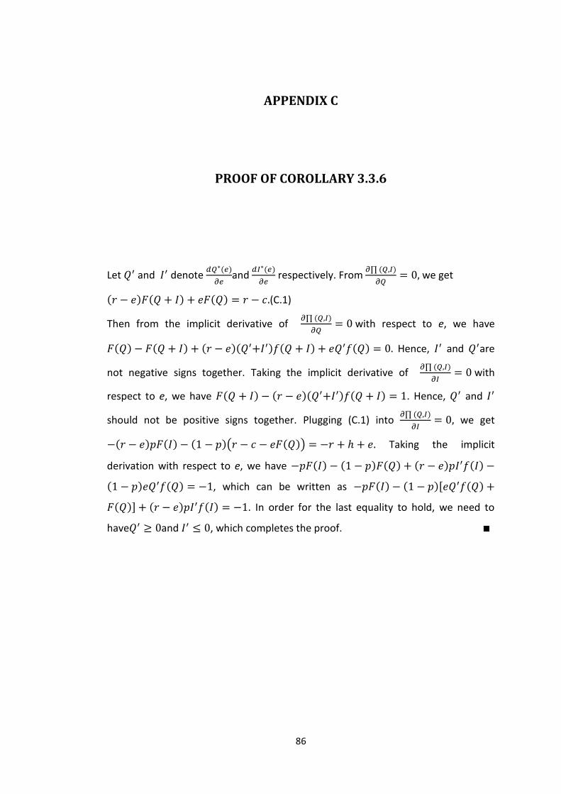
86

APPENDIX C


Let and denote

and

respectively. From

we get

(C.1)


with respect to e, we have

Hence, and are

not negative signs together. Taking the implicit derivative of

with

respect to e, we have . Hence, and

should not be positive signs together. Plugging (C.1) into

we get

( ) Taking the implicit

derivation with respect to e, we have

, which can be written as [

] . In order for the last equality to hold, we need to

have and , which completes the proof.

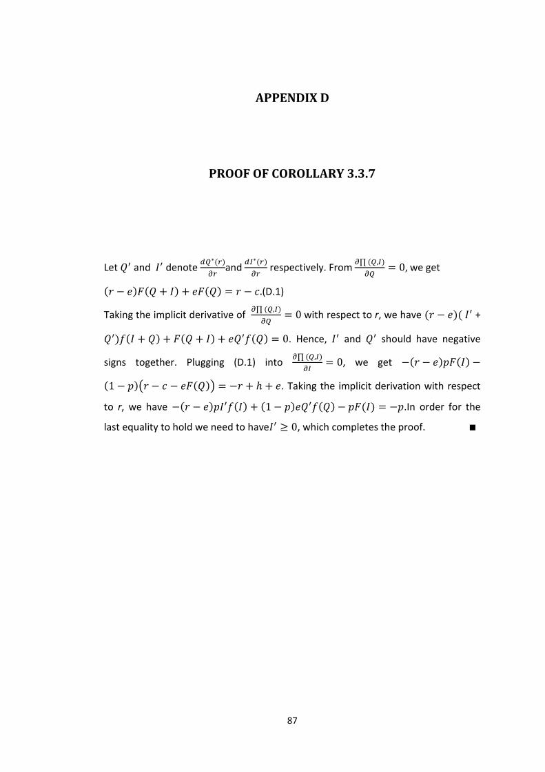
87

APPENDIX D


Let and denote

and

respectively. From

we get

(D.1)

Taking the implicit derivative of

with respect to r, we have +

. Hence, and should have negative

signs together. Plugging (D.1) into

, we get

( ) . Taking the implicit derivation with respect

to r, we have .In order for the

last equality to hold we need to have , which completes the proof.

88

APPENDIX E


From corollary 4.3.1, we have two different alternatives solution to ; for

, (

) [

] which

can be written as (

) [

], otherwise

{ (

) }. In either case, we can argue that is non-decreasing in

the reservation cost, h and exercise cost, c. From corollary 4.3.1, we have two

different alternative solutions to , for , max{ [

] } and for

, max{ [

] } which can be written as

max{ [

] } . In either case, we can argue that is non-increasing

in the reservation cost, h, and exercise cost, c which completes the proof.

89

APPENDIX F


From corollary 4.3.1, we have two different alternatives solution to ; for

, (

) [

] which

can be written as (

) [

], otherwise

{ (

) }. In either case, we can argue that is non-increasing in

the disruption probability, p. From corollary 4.3.1, we have two different

alternative solutions to , for , max{ [

] } and for ,

max{ [

] } which can be written as max{ [

] } .

In either case, we can argue that is non-decreasing in the disruption probability,

p, which completes the proof.

90

APPENDIX G

THE OPTIMAL RESULTS FOR THE PARAMETER SENSITIVITY

ANALYSIS

Table G.1: Optimal Results for the problem instances when is increased

NO INFORMATION

p Profit Q I

0,01 12112,68 109,9414 0

0,05 11623,28 109,9414 0

0,1 11143,94 22,38281 87,55859

0,15 11106,34 13,76953 96,17676

0,2 11088,61 10,61523 99,33105

0,25 11077,7 8,769531 101,1719

0,3 11070,17 7,529297 102,417

0,35 11064,63 6,611328 103,3301

0,4 11060,36 5,908203 104,0332

0,45 11056,9 5,35 104,59

0,5 11054,1 4,89 105,053

0,55 11051,85 4,5 105,43

0,6 11049,89 4,17 105,76

0,65 11048,2 3,89 106,04

0,7 11046,74 3,65 106,28

0,75 11045,46 3,43 106,5

0,8 11044,33 3,25 106,68

0,85 11043,32 3,07 106,86

0,9 11042,4 2,92 107,02

PARTIAL INFORMATION

p Profit Q I

0,01 12112,68 109,9446 0

0,05 11707,14 109,9446 88,89229

0,1 11651,9 109,9446 99,16348

0,15 11611,73 109,9446 101,9621

0,2 11575,09 109,9446 103,4069

91

Table G.1: Optimal Results for the problem instances when is increased (cont’d)

p Profit Q I

0,25 11539,92 109,9446 104,3073

0,3 11505,52 109,9446 104,927

0,35 11471,56 109,9446 105,3815

0,4 11437,89 109,9446 105,7297

0,45 11404,4 109,945 106

0,5 11371,07 109,945 106,22

0,55 11337,8 109,945 106,41

0,6 11304,6 109,945 106,57

0,65 11271,5 109,945 106,7

0,7 11238,5 109,945 106,82

0,75 11205,52 109,945 106,92

0,8 11172,5 109,945 107

0,85 11139,59 109,945 107,09

0,9 11106,66 109,945 107,15

FULL INFORMATION

p Profit Q I

0,01 12282,47 95,54408 22,9796

0,05 11951,33 91,58379 90,32583

0,1 11894,95 91,58379 102,1043

0,15 11856,87 91,58379 105,8946

0,2 11823,84 91,58379 108,1222

0,25 11793,19 91,58379 109,6742

0,3 11763,91 91,58379 110,8533

0,35 11735,51 91,58379 111,7976

0,4 11707,74 91,58379 112,5816

0,45 11680,41 91,58379 113,24

0,5 11653,44 91,58379 113,82

0,55 11626,74 91,58379 114,34

0,6 11600,26 91,58379 114,79

0,65 11573,96 91,58379 115,21

0,7 11547,81 91,58379 115,58

0,75 11521,79 91,58379 115,93

0,8 11495,89 91,58379 116,24

0,85 11470,08 91,58379 116,54

0,9 11444,35 91,58379 116,81

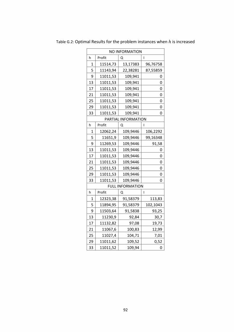
92


NO INFORMATION

h Profit Q I

1 11514,73 13,17383 96,76758

5 11143,94 22,38281 87,55859

9 11011,53 109,941 0

13 11011,53 109,941 0

17 11011,53 109,941 0

21 11011,53 109,941 0

25 11011,53 109,941 0

29 11011,53 109,941 0

33 11011,53 109,941 0

PARTIAL INFORMATION

h Profit Q I

1 12062,24 109,9446 106,2292

5 11651,9 109,9446 99,16348

9 11269,53 109,9446 91,58

13 11011,53 109,9446 0

17 11011,53 109,9446 0

21 11011,53 109,9446 0

25 11011,53 109,9446 0

29 11011,53 109,9446 0

33 11011,53 109,9446 0

FULL INFORMATION

h Profit Q I

1 12323,38 91,58379 113,83

5 11894,95 91,58379 102,1043

9 11503,64 91,5838 93,25

13 11230,9 92,84 30,7

17 11132,82 97,08 19,73

21 11067,6 100,83 12,99

25 11027,4 104,71 7,01

29 11011,62 109,52 0,52

33 11011,52 109,94 0

93


NO INFORMATION

c Profit Q I

22 11209,93 110,5078 0

23 11165,96 27,00195 83,22266

24 11143,94 22,38281 87,55859

25 11125,22 19,35547 90,32227

26 11108,94 16,91406 92,5

27 11094,69 14,78516 94,37012

28 11082,27 12,84668 96,05469

29 11071,54 11,02051 97,63672

30 11062,41 9,24 99,16

31 11054,88 7,509766 100,6689

32 11048,9 5,761719 102,1875

PARTIAL INFORMATION

c Profit Q I

22 11850,3 110,5084 99,16348

23 11750,97 110,2224 99,16348

24 11651,9 109,9446 99,16348

25 11553,07 109,6742 99,16348

26 11454,48 109,4107 99,16348

27 11356,13 109,1537 99,16348

28 11258 108,9025 99,16348

29 11160,1 108,6568 99,16348

30 11062,41 9,25 99,1635

31 11054,88 7,511597 100,6688

32 11048,9 5,75942 102,1897

FULL INFORMATION

c Profit Q I

22 12061,75 93,77075 102,1043

23 11977,86 92,72087 102,1043

24 11894,95 91,58379 102,1043

25 11813,12 90,32578 102,1043

26 11732,5 88,89229 102,1043

27 11653,29 87,18449 102,1043

28 11575,83 84,98917 102,1043

29 11500,81 81,66084 102,1043

30 11420,37 50 102,1

31 11420,38 50 102,1043

32 11424,7 19,86061 104,0792

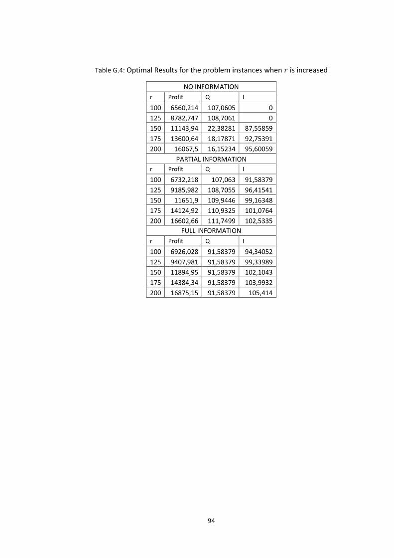
94


NO INFORMATION

r Profit Q I

100 6560,214 107,0605 0

125 8782,747 108,7061 0

150 11143,94 22,38281 87,55859

175 13600,64 18,17871 92,75391

200 16067,5 16,15234 95,60059

PARTIAL INFORMATION

r Profit Q I

100 6732,218 107,063 91,58379

125 9185,982 108,7055 96,41541

150 11651,9 109,9446 99,16348

175 14124,92 110,9325 101,0764

200 16602,66 111,7499 102,5335

FULL INFORMATION

r Profit Q I

100 6926,028 91,58379 94,34052

125 9407,981 91,58379 99,33989

150 11894,95 91,58379 102,1043

175 14384,34 91,58379 103,9932

200 16875,15 91,58379 105,414

95


NO INFORMATION

e Profit Q I

18 0 0 0

20 12126,35 2,441406 107,5

22 11915,41 6,357422 103,584

24 11711,69 9,77 100,16

26 11514,73 13,17383 96,76758

28 11324,9 17,00195 92,93945

30 11143,94 22,38281 87,55859

32 11011,53 109,9414 0

PARTIAL INFORMATION

e Profit Q I

18 0 0 0

20 12126,35 2,445974 107,4986

22 11915,41 6,360064 103,5845

24 11711,7 9,775 100,16

26 11691,7 109,9446 99,83288

28 11671,76 109,9446 99,49846

30 11651,9 109,9446 99,16348

32 11632,1 109,9446 98,82755

e Profit Q I

FULL INFORMATION

18 0 0 0

20 12386,62 6,307068 112,389

22 12206,17 14,79382 106,7449

24 12017,89 50 102,61

26 11975,54 85,73921 102,4501

28 11933,05 89,3243 102,2797

30 11894,95 91,58379 102,1043

32 11859,67 93,2551 101,9236

96


NO INFORMATION

Profit Q I

5 11321,97 11,19141 93,7793

10 11143,94 22,38281 87,55859

15 10965,91 33,59 81,32

20 10787,88 44,76563 75,11719

25 10609,85 55,97 68,88

30 10431,82 67,1875 62,65625

PARTIAL INFORMATION

Profit Q I

5 11845,95 104,9723 99,58174

10 11651,9 109,9446 99,16348

15 11457,84 114,91 98,74

20 11263,79 119,8892 98,32695

25 11069,74 124,86 97,9

30 10875,69 129,83 97,49046

Profit Q I

FULL INFORMATION

5 11958,4 95,79189 101,0521

10 11894,95 91,58379 102,1043

15 11831,5 87,37 103,156

20 11768,21 83,16936 104,2115

25 11713,54 79,08 105,46

30 11673,87 75,8368 108,1039

Documents

ANALYSIS OF AN OPTIONS CONTRACT IN A DUAL SOURCING SUPPLY …