Embed Size (px)
Citation preview

ANALYSIS OF ALTERNATIVE DIGIT SETS FOR NONADJACENT
REPRESENTATIONS
CLEMENS HEUBERGER‡ AND HELMUT PRODINGER∗
Abstract. It is known that every positive integer n can be represented as a finite sumof the form
∑iai2
i, where ai ∈ {0, 1,−1} and no two consecutive ai’s are non-zero(“nonadjacent form”, NAF). Recently, Muir and Stinson [12, 13] investigated other digitsets of the form {0, 1, x}, such that each integer has a nonadjacent representation (such anumber x is called admissible). The present paper continues this line of research.
The topics covered include transducers that translate the standard binary representa-tion into such a NAF and a careful topological study of the (exceptional) set (which is offractal nature) of those numbers where no finite look-ahead is sufficient to construct theNAF from left-to-right, counting the number of digits 1 (resp. x) in a (random) represen-tation, and the non-optimality of the representations if x is different from 3 or −1.
1. Introduction
Redundant number systems have been studied by many people, and for various reasons.Probably the most famous one uses the base 2, but instead of the traditional digits 0, 1, itallows a third digit −1. One can make this system unique by superimposing a condition:no two adjacent digits different from zero are permitted. This non-adjacent-form (“NAF”)goes back (at least) to Reitwiesner [15]. For pointers to the earlier literature we refer thereader to [10] and [7].
Recently, Muir and Stinson [12, 13] asked for other sets of digits, in particular of theform {0, 1, x}, such that every (positive) integer has a unique representation using thesedigits, base 2, and obeying again the condition that two adjacent digits cannot both bedifferent from zero.
The present paper analyzes their number systems with respect to frequencies of digits,description of characteristic sets and similar questions. Our main focus is to provide resultsfor general x as much as possible; we give explicit results as well as algorithms to computesome characteristic quantities for specific x.
We summarize here what follows in the later sections.In order to describe the digits x that work, we define a suitable graph. The answer
depends on whether each node can be reached from the starting node. We propose
‡ This paper was written while the first author was a visitor at the John Knopfmacher Centre forApplicable Analysis and Number Theory, School of Mathematics, University of the Witwatersrand, Jo-hannesburg. He thanks the centre for its hospitality. He was also supported by the grant S8307-MAT ofthe Austrian Science Fund.
∗ This author is supported by the grant NRF 2053748 of the South African National ResearchFoundation.
1
2 C. HEUBERGER AND H. PRODINGER
an O(|x|)-time algorithm for this decision. The list of admissible numbers x starts like3,−1,−5,−13, . . . (they must all be ≡ 3 mod 4).
We then define transducers (finite automata with output) that translate the standardbinary representation into a NAF using digits {0, 1, x} by reading the input word fromright to left (thus starting with the least significant digit). Such a transducer has at most|x| + 4 states. It can be constructed even for such x’s that don’t lead to NAFs; in suchcases, not every number has a representation, and one can “see” from the transducer whenthis happens. (For the standard NAF, such a transducer is of course well known.)
One of the advantages of the (standard) NAF, especially for applications in cryptogra-phy, is, that many digits are zero “on average.” To be more precise, if one considers alladmissible words of length N , with digits (letters) from the set {0, 1,−1}, then a randomword has on average N
6digits ‘1’ resp. ‘−1’ and 2N
3zeros. Interestingly, these frequencies
persist even in the general case, with error terms depending on the extra digit x; in prin-ciple (for any particular x), they can be computed. The variance follows a similar pattern,with the constant 1
6being replaced by 11
108. From this one can conclude that the underlying
distribution is Gaussian.For various reasons (on-line computations!) it would be nice to generate the NAF when
reading the digits of the binary expansion from left-to-right. It is known for the standardcase x = −1 that this is not possible, but there exist equivalent representations (withrespect to the large number of zeros, i.e., small “Hamming weight”). There are alwayssituations where a finite look-ahead will not be sufficient to decide which digit should betaken. We scale this exceptional set B down to the unit interval and study it as a functionof the length of the look-ahead. While this set is just { 1
6, 2
6, 4
6, 5
6} in the standard instance,
we enter the realm of fractals for x = −5,−13, . . . . The (Lebesgue-) measure of B is zero,but its Hausdorff dimension is positive and strictly less than 1. A similar situation occurredin the study of joint expansions in Grabner, Heuberger, and Prodinger [5]. For particularx, the Hausdorff dimension can be explicitly computed from the dominant eigenvalue ofthe adjacency matrix of a certain auxiliary automaton, but it is quite challenging to saysomething in general. We manage, however, to derive nontrivial lower and upper bounds.
As already mentioned, for x = −1, the NAF is optimal, as there is no representation ofany integer with fewer nonzero digits. We show in an algorithmic fashion that this is alsotrue for x = 3. This is no longer true for the other possible values of x. In most cases, thenumber 3 serves as a counter example; in a few exceptional cases one must take anotherone. As a byproduct of our analysis, we can describe (for x = 1 resp. x = 3) all optimalrepresentations; recall that in these cases a representation of an integer m is optimal if ithas the same number on nonzero digits as the NAF of m. These representations can bedescribed by finite automata.
It is always beneficial in order to understand how the arithmetic of a number systemworks to understand first how addition of 1 (or any other fixed integer) works. Knuth’sbook [10] has several such examples. Here, we confine ourselves to the transducer describingthe addition of 1 in the instance x = −5.

ANALYSIS OF ALTERNATIVE DIGIT SETS FOR NONADJACENT REPRESENTATIONS 3
For the standard NAF case (x = −1) it is possible to give an explicit formula for thedigits of the expansion, cf. Prodinger [14]. This is somehow a reflection of the fact thatthe above mentioned exceptional set is so simple. In the instance x = −5, there is stillan explicit formula for the digits. However, it sometimes predicts a nonzero digit when itactually is zero, but is correct otherwise. This corresponds to Figure 9, where one can seethat the intervals that contain green resp. blue points, are separated. For other values ofx nothing like that exists anymore.
Before entering into the details, we will fix a minimum amount of notation. Let n be aninteger and D ⊂ Z. A (binary) D-expansion of n is a sequence (. . . , d2, d1, d0) ∈ D
�0 such
that only finitely many digits are nonzero and such that n =∑
j≥0 dj2j. The standard
binary expansion of a nonnegative integer n is its unique {0, 1}-expansion. We will usuallydenote sequences by boldface letters. Where appropriate, we will also think about D-expansions as finite or infinite words over the alphabet D. By value(. . . , d2, d1, d0), wedenote
∑j≥0 dj2
j. The position of the most significant digit MSB(d) is max{j : dj 6= 0}.
2. Nonadjacent Digit Sets
We recall some definitions of Muir and Stinson [12, 13].
Definition 1. (1) Let 0 ∈ D ⊂ Z and n ∈ Z. Then a D-expansion η of n is called aD-nonadjacent form (D-NAF) of n, if
ηjηj+1 = 0 for all j ≥ 0.
(2) Let 0 ∈ D ⊂ Z. If there is a D-NAF for every positive integer n, then D is calleda nonadjacent digit set (NADS).
Muir and Stinson [12, 13] study digit sets D = {0, 1, x} for integers x. The followingresults have been proved in their paper:
Proposition 2. Let D = {0, 1, x}.(1) If D is a NADS, then x ≡ 3 (mod 4).(2) If x ≡ 3 (mod 4), then each positive integer has at most one D-NAF.(3) The only NADS D = {0, 1, x} with positive x is {0, 1, 3}.
Definition 3. Let D = {0, 1, x} with x ≡ 3 (mod 4). Then we define η0 : Z → D andr : Z→ Z by setting
η0(n) :=
0, if n ≡ 0 (mod 2),
1, if n ≡ 1 (mod 4),
x, if n ≡ 3 (mod 4),
r(n) :=n− η0(n)
2.
It is easily seen (cf. Muir and Stinson [12, 13]) that n ∈ N admits a D-NAF if and only ifr(n) admits a D-NAF and that if (. . . , η′1, η
′0) is the D-NAF of r(n) then (. . . , η′1, η
′0, η0(n))
is the D-NAF of n. (Note that r(n) is even if n is odd).Since r(n) < n for all positive n 6≡ 3 (mod 4) and r2(n) := r(r(n)) < n for all positive
n ≡ 3 (mod 4) with n > |x| /3, the set D is a NADS if and only if all 0 < n ≤ |x| /3 withn ≡ 3 (mod 4) have a D-NAF.

4 C. HEUBERGER AND H. PRODINGER
Proposition 4. Let D = {0, 1, x} with x < 0 and x ≡ 3 (mod 4). Define the directedgraph G := (V,A) by V = {0, . . . , b|x| /3c} and
A := {(m,n) ∈ V 2 : n ∈ {2m, 4m+ 1, 4m+ x}}.Then D is a NADS if and only if every n ∈ V is reachable from 0.
Proof. We observe that if 0 6= n ∈ V , then there is exactly one edge with head n, namely(ri(n), n), where i = (n mod 2) + 1. Therefore, there is a path1 from 0 to n if and only ifn has a D-NAF. �
Therefore, we may check whether a set D is a NADS by simple breadth-first search (cf.Algorithm 1).
Algorithm 1 Check for NADS
Input: D = {0, 1, x} with x < 0 and x ≡ 3 (mod 4)Output: Decision, whether D is a NADSS ← (0)c← 1while S 6= () do
m← First element of SRemove m from ST ← {2m, 4m+ 1, 4m+ x} ∩ {0, . . . , b|x| /3c}c← c+ #TAppend T to S
end while
if c = b|x| /3)c+ 1 then
Return(True)else
Return(False)end if
It is clear that the run-time of this algorithm is O(|x|). Muir and Stinson [12, 13] givea list of all NADS {0, 1, x} with |x| ≤ 10 000. The list starts with
3,−1,−5,−13,−17,−25,−29,−37,−53,−61,−65, . . .
They also gave some necessary and some sufficient conditions on x such that {0, 1, x} is aNADS.
We remark that for negative integers n, we always have r(n) > n if x < 0. This impliesthat for some finite positive k, we have rk(n) ≥ 0.
Proposition 5. Let D := {0, 1, x} with x < 0 be a NADS. Then every integer n ∈ Z hasa D-NAF.
1In this paper, a path in a transducer, in an automaton or in a directed graph is not required to havedistinct vertices.
ANALYSIS OF ALTERNATIVE DIGIT SETS FOR NONADJACENT REPRESENTATIONS 5
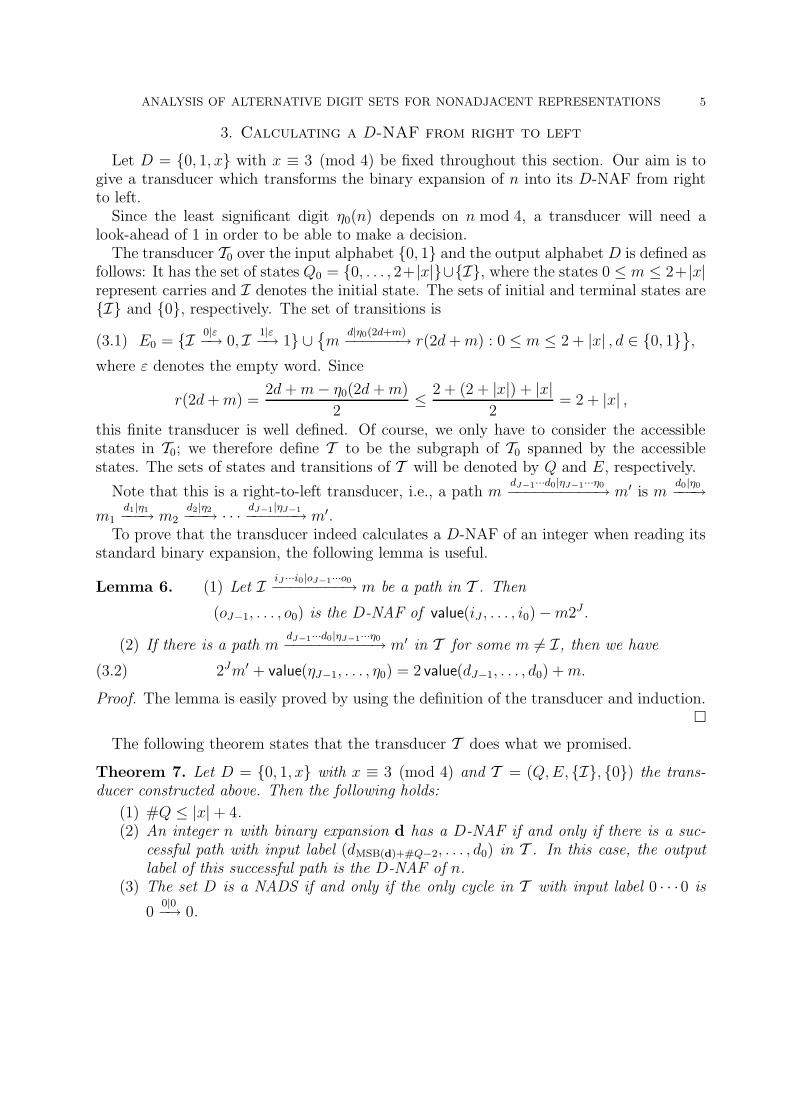
3. Calculating a D-NAF from right to left
Let D = {0, 1, x} with x ≡ 3 (mod 4) be fixed throughout this section. Our aim is togive a transducer which transforms the binary expansion of n into its D-NAF from rightto left.
Since the least significant digit η0(n) depends on n mod 4, a transducer will need alook-ahead of 1 in order to be able to make a decision.
The transducer T0 over the input alphabet {0, 1} and the output alphabet D is defined asfollows: It has the set of states Q0 = {0, . . . , 2+|x|}∪{I}, where the states 0 ≤ m ≤ 2+|x|represent carries and I denotes the initial state. The sets of initial and terminal states are{I} and {0}, respectively. The set of transitions is
(3.1) E0 = {I 0|ε−→ 0, I 1|ε−→ 1} ∪{m
d|η0(2d+m)−−−−−−→ r(2d+m) : 0 ≤ m ≤ 2 + |x| , d ∈ {0, 1}},
where ε denotes the empty word. Since
r(2d+m) =2d+m− η0(2d+m)
2≤ 2 + (2 + |x|) + |x|
2= 2 + |x| ,
this finite transducer is well defined. Of course, we only have to consider the accessiblestates in T0; we therefore define T to be the subgraph of T0 spanned by the accessiblestates. The sets of states and transitions of T will be denoted by Q and E, respectively.
Note that this is a right-to-left transducer, i.e., a path mdJ−1···d0|ηJ−1···η0−−−−−−−−−−→ m′ is m
d0|η0−−−→m1
d1|η1−−−→ m2d2|η2−−−→ · · · dJ−1|ηJ−1−−−−−−→ m′.
To prove that the transducer indeed calculates a D-NAF of an integer when reading itsstandard binary expansion, the following lemma is useful.
Lemma 6. (1) Let I iJ ···i0|oJ−1···o0−−−−−−−−→ m be a path in T . Then
(oJ−1, . . . , o0) is the D-NAF of value(iJ , . . . , i0)−m2J .
(2) If there is a path mdJ−1···d0|ηJ−1···η0−−−−−−−−−−→ m′ in T for some m 6= I, then we have
(3.2) 2Jm′ + value(ηJ−1, . . . , η0) = 2 value(dJ−1, . . . , d0) +m.
Proof. The lemma is easily proved by using the definition of the transducer and induction.�
The following theorem states that the transducer T does what we promised.
Theorem 7. Let D = {0, 1, x} with x ≡ 3 (mod 4) and T = (Q,E, {I}, {0}) the trans-ducer constructed above. Then the following holds:
(1) #Q ≤ |x|+ 4.(2) An integer n with binary expansion d has a D-NAF if and only if there is a suc-
cessful path with input label (dMSB(d)+#Q−2, . . . , d0) in T . In this case, the outputlabel of this successful path is the D-NAF of n.
(3) The set D is a NADS if and only if the only cycle in T with input label 0 · · ·0 is
00|0−→ 0.

6 C. HEUBERGER AND H. PRODINGER
Proof. (1) Follows from the definition.(2) Assume that n > 0 has a D-NAF η and a standard binary expansion d. Let
J := max{MSB(η),MSB(d)}. Consider the path I dJ+2dJ+1dJ ···d0|oJ+1oJ ···o0−−−−−−−−−−−−−−−−→ m inT . From Lemma 6 we conclude that n − m2J+2 has a D-NAF (oJ+1, oJ , . . . , o0).This implies that value(ηJ , . . . , η0) ≡ value(oJ+1, . . . , o0) (mod 2J+2). Since bothexpansions are D-NAFs, we infer that ηj = oj for 0 ≤ j ≤ J . This yieldsoJ+12
J+1 = −m2J+2 from which we conclude that oJ+1 = m = 0. This implies
that I dJ+2dJ+1dJ ···d0|0ηJ ···η0−−−−−−−−−−−−−−→ 0 is a successful path in T . We will prove that thelength of a successful path is at most MSB(d) + #Q − 1 after proving the thirdpart of the theorem.
On the other hand, if there is some successful path, Lemma 6 shows that itcorresponds to a D-NAF of the value of its input.
(3) When processing the binary expansion of n on the transducer, we can distinguishbetween two phases: in the first phase, we read “significant” input, in the secondphase, we just read leading zeros of the binary expansion. If we reach the terminalstate 0 in this second phase, we are successful and got a D-NAF of our input.
However, if we enter a cycle in the second phase apart from the trivial cycle 00|0−→ 0,
it is clear that we will never reach the terminal state, i.e., there is no D-NAF.This implies that after reading dMSB(d), we will reach each of the states Q\{I, 0}
at most once, hence we need at most #Q − 2 leading zeros to reach the terminalstate 0.
�
For x = 3, x = −1, x = −5, x = −9, and x = −13, the transducers T are shown in
Figures 1, 2, 3, 4, and 5, respectively. Note that for x = −9, there is a cycle 30|9−→ 6
0|0−→ 3,therefore, {0, 1,−9} is not a NADS.
I
0 1
0|ε
1|ε
0|0
1|00|1, 1|3
Figure 1. Transducer T for calculating the {0, 1, 3}-NAF of n from itsstandard binary expansion from right to left.

ANALYSIS OF ALTERNATIVE DIGIT SETS FOR NONADJACENT REPRESENTATIONS 7
I
0 1 2
0|ε
1|ε
0|0
1|00|1
1|10|0
1|0
Figure 2. Transducer T for calculating the {0, 1,−1}-NAF of n from itsstandard binary expansion from right to left.
I
0 1
4
2
3
0|ε
1|ε
0|0
1|00|1
1|5 0|0
1|0
0|0
1|0
0|5
1|1
Figure 3. Transducer T for calculating the {0, 1,−5}-NAF of n from itsstandard binary expansion from right to left.
In some parts of this paper, we will study the input automaton A of T , i.e., we onlyconsider the input labels of the transitions in T . By construction, the automaton A isdeterministic. We will use the notation m′ = (dJ−1 · · ·d0) ·m for the transition functionin this automaton, which means that there is a path in A from m to m′ with (input)label (dJ−1 · · ·d0). Furthermore, we will apply these transitions to sets of states also, i.e.(dJ−1 · · ·d0) ·M := {(dJ−1 · · ·d0) ·m : m ∈M} for M ⊆ Q.
The following lemma will be used several times:
Lemma 8. Let x < 0,
(3.3) k0 := 2 + max{MSB(η(n)) : −2 ≤ n ≤ 2 + |x|}

8 C. HEUBERGER AND H. PRODINGER
I
0 1
6
34
2
0|ε
1|ε0|0
1|00|1
1|9
0|01|0 0|9
1|1
1|0
0|0
0|0
1|0
Figure 4. Transducer T for calculating the {0, 1,−9}-NAF of n from itsstandard binary expansion from right to left.
and m ∈ Q \ {I}. Then for any k ≥ k0, we have
(0k) ·m = 0,
(1k) ·m = 2,
where dk means the word consisting of k repetitions of the letter d.
Proof. Let d ∈ {0, 1}. We consider the path
mdk|ηk−1···η0−−−−−−→ m′
in T . By (3.2), we have
(3.4) 2km′ + value(ηk−1 · · · η0) = 2d(2k − 1) +m = d2k+1 +m− 2d.
By definition of k0, the D-NAF η′ of m− 2d satisfies MSB(η′) ≤ k− 2. Then (3.4) implies
that value(ηk−1 · · · η0) ≡ value(η′k−1 · · · η′0) (mod 2k), which yields ηj = η′j for 0 ≤ j ≤ k−2.Inserting this in (3.4) we immediately see that ηk−1 = 0 and m′ = 2d. �
Furthermore, we can also construct a transducer T0 which takes an arbitrary binary{0, 1, x}-expansion and transforms it to the D-NAF: The set of states Q0 is {I}∪ {−2 |x|,

ANALYSIS OF ALTERNATIVE DIGIT SETS FOR NONADJACENT REPRESENTATIONS 9
I
0 1
8
4
5
2
3
10
6
0|ε
1|ε0|0
1|00|1
1|13
0|0
1|0
0|0
1|0
0|1
1|13
0|0
1|0
0|13
1|1
0|01|0
1|00|0
Figure 5. Transducer T for calculating the {0, 1,−13}-NAF of n from itsstandard binary expansion from right to left.
. . . , |x| + 2}, the set of transitions E0 is
(3.5) E0 = {I 0|ε−→ 0, I 1|ε−→ 1, I x|ε−→ x}
∪{m
d|η0(2d+m)−−−−−−→ r(2d+m) : −2 |x| ≤ m ≤ 2 + |x| , d ∈ {0, 1, x}}.
The transducer T is obtained by removing inaccessible states. The transducers T for x = 3and x = −1 are shown in Figures 13 and 15, respectively.
4. Frequency of digits
Let D = {0, 1, x} be a fixed NADS. We denote the D-NAF of a nonnegative integer nby η(n). For d ∈ {1, x}, we denote the number of occurrences of the digit d in the D-NAFof n ∈ N0 by
(4.1) fd(n) :=∑
j≥0
[ηj(n) = d] ,
10 C. HEUBERGER AND H. PRODINGER
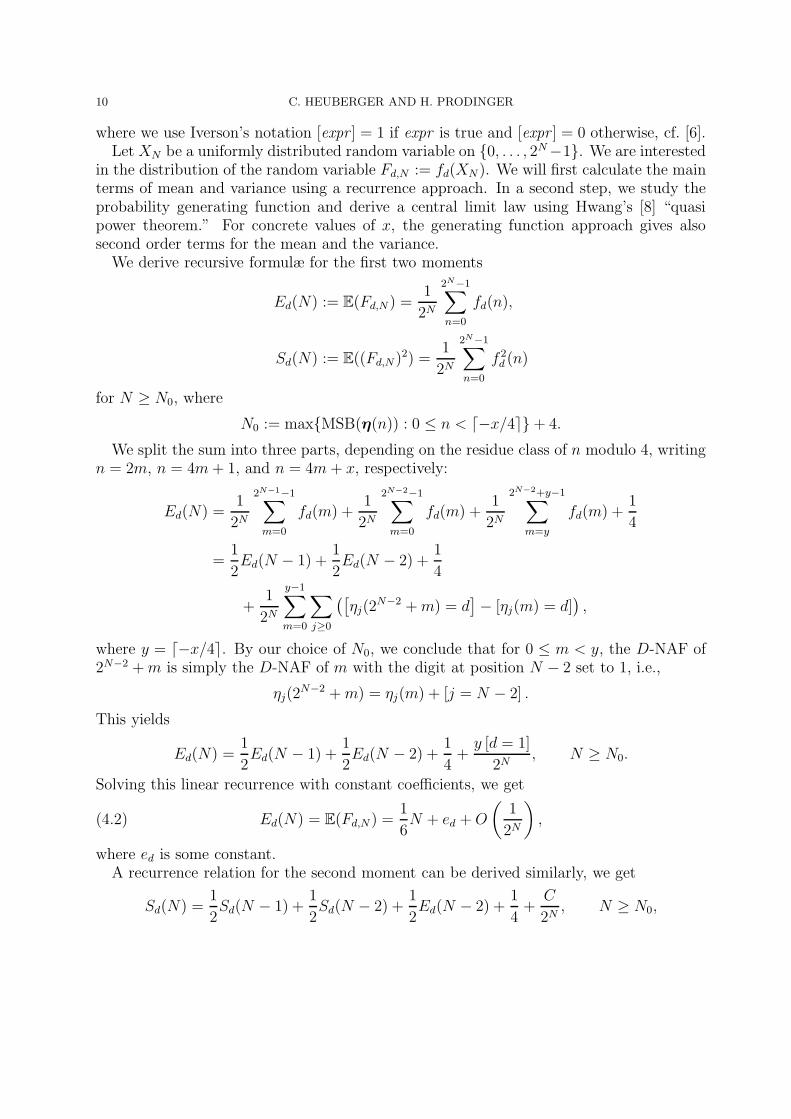
where we use Iverson’s notation [expr ] = 1 if expr is true and [expr ] = 0 otherwise, cf. [6].Let XN be a uniformly distributed random variable on {0, . . . , 2N−1}. We are interested
in the distribution of the random variable Fd,N := fd(XN ). We will first calculate the mainterms of mean and variance using a recurrence approach. In a second step, we study theprobability generating function and derive a central limit law using Hwang’s [8] “quasipower theorem.” For concrete values of x, the generating function approach gives alsosecond order terms for the mean and the variance.
We derive recursive formulæ for the first two moments
Ed(N) := E(Fd,N ) =1
2N
2N−1∑
n=0
fd(n),
Sd(N) := E((Fd,N )2) =1
2N
2N−1∑
n=0
f 2d (n)
for N ≥ N0, where
N0 := max{MSB(η(n)) : 0 ≤ n < d−x/4e}+ 4.
We split the sum into three parts, depending on the residue class of n modulo 4, writingn = 2m, n = 4m+ 1, and n = 4m + x, respectively:
Ed(N) =1
2N
2N−1−1∑
m=0
fd(m) +1
2N
2N−2−1∑
m=0
fd(m) +1
2N
2N−2+y−1∑
m=y
fd(m) +1
4
=1
2Ed(N − 1) +
1
2Ed(N − 2) +
1
4
+1
2N
y−1∑
m=0
∑
j≥0
([ηj(2
N−2 +m) = d]− [ηj(m) = d]
),
where y = d−x/4e. By our choice of N0, we conclude that for 0 ≤ m < y, the D-NAF of2N−2 +m is simply the D-NAF of m with the digit at position N − 2 set to 1, i.e.,
ηj(2N−2 +m) = ηj(m) + [j = N − 2] .
This yields
Ed(N) =1
2Ed(N − 1) +
1
2Ed(N − 2) +
1
4+y [d = 1]
2N, N ≥ N0.
Solving this linear recurrence with constant coefficients, we get
(4.2) Ed(N) = E(Fd,N ) =1
6N + ed +O
(1
2N
),
where ed is some constant.A recurrence relation for the second moment can be derived similarly, we get
Sd(N) =1
2Sd(N − 1) +
1
2Sd(N − 2) +
1
2Ed(N − 2) +
1
4+
C
2N, N ≥ N0,

ANALYSIS OF ALTERNATIVE DIGIT SETS FOR NONADJACENT REPRESENTATIONS 11
where C = [d = 1]∑y−1
m=0(2fd(m) + 1) is a constant. Inserting (4.2) (with undeterminedconstants), we again get a linear recurrence with constant coefficients. Solving it, we get
Sd(N) = E((Fd,N )2) =1
36N2 +
(11
108+ed
3
)N + (vd + e2d) +O
(N
2N
)
for some constant vd. Subtracting (Ed(N))2, we get
(4.3) V(Fd,N) = E((Fd,N )2)− (E(Fd,N ))2 =11
108N + vd +O
(N
2N
).
We now consider the probability generating function
Gd(Y, Z) =∑
N≥0
∑
m≥0
P(Fd,N = m)Y mZN .
We define the (#Q×#Q)-matrices Ad := Ad(Y ) = (aij)i,j∈Q and Bd = Bd(Y ) = (bij)i,j∈Q
by
aij =∑
v∈{0,1}
iv|η−→j∈E
1
2Y [η=d], bij =
{Y [η=d], if there is a transition i
0|η−→ j ∈ E,0, otherwise,
where the rows and columns of Ad and Bd are ordered as I, 0, 1, . . .. Then Gd(Y, Z) canbe expressed as
Gd(Y, Z) = (1, 0, . . . , 0)(I − AdZ)−1B#Q−2d (0, 1, 0, . . . , 0)t,
where the factor B#Q−2d ensures that we come back to the terminal state 0. For concrete
x, Gd can be calculated explicitly, for instance, we have
G1(Y, Z) =16− 8Z + 8Y Z − 4Z2 − Y Z4 + Y 2Z4
2(−2 + Z)(−4 + 2Z + Z2 + Y Z2),
G−5(Y, Z) =−(8 + 4Z − Y Z3 + Y 2Z3)
2(−4 + 2Z + Z2 + Y Z2)
for x = −5. Then we have
E(Fd,N ) = [ZN ]
(∂Gd
∂Y
∣∣∣∣Y =1
),
V(Fd,N) = [ZN ]
(∂2Gd
∂Y 2
∣∣∣∣Y =1
)+ E(Fd,N)− (E(Fd,N ))2.
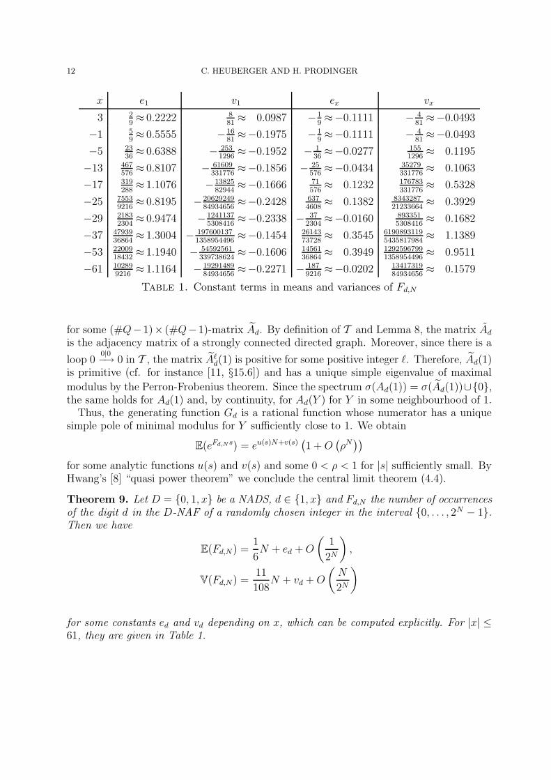
For the first ten values of x, we calculated means and variances by this approach. Com-paring with (4.2) and (4.3) for the first few values of x gives the constants ed and vd inTable 1.
From the definition (3.1) of the transducer T it is clear that
Ad(Y ) =
(0 1 1 0 . . . 0
0 Ad(Y )
)
12 C. HEUBERGER AND H. PRODINGER
x e1 v1 ex vx
3 29≈ 0.2222 8
81≈ 0.0987 − 1
9≈−0.1111 − 4
81≈−0.0493
−1 59≈ 0.5555 − 16
81≈−0.1975 − 1
9≈−0.1111 − 4
81≈−0.0493
−5 2336≈ 0.6388 − 253
1296≈−0.1952 − 1
36≈−0.0277 155
1296≈ 0.1195
−13 467576≈ 0.8107 − 61609
331776≈−0.1856 − 25
576≈−0.0434 35279
331776≈ 0.1063
−17 319288≈ 1.1076 − 13825
82944≈−0.1666 71
576≈ 0.1232 176783
331776≈ 0.5328
−25 75539216≈ 0.8195 − 20629249
84934656≈−0.2428 637
4608≈ 0.1382 8343287
21233664≈ 0.3929
−29 21832304≈ 0.9474 − 1241137
5308416≈−0.2338 − 37
2304≈−0.0160 893351
5308416≈ 0.1682
−37 4793936864
≈ 1.3004 − 1976001371358954496
≈−0.1454 2614373728
≈ 0.3545 61908931195435817984
≈ 1.1389
−53 2200918432
≈ 1.1940 − 54592561339738624
≈−0.1606 1456136864
≈ 0.3949 12925967991358954496
≈ 0.9511
−61 102899216≈ 1.1164 − 19291489
84934656≈−0.2271 − 187
9216≈−0.0202 13417319
84934656≈ 0.1579
Table 1. Constant terms in means and variances of Fd,N
for some (#Q− 1)× (#Q− 1)-matrix Ad. By definition of T and Lemma 8, the matrix Ad
is the adjacency matrix of a strongly connected directed graph. Moreover, since there is a
loop 00|0−→ 0 in T , the matrix A`
d(1) is positive for some positive integer `. Therefore, Ad(1)is primitive (cf. for instance [11, §15.6]) and has a unique simple eigenvalue of maximal
modulus by the Perron-Frobenius theorem. Since the spectrum σ(Ad(1)) = σ(Ad(1))∪{0},the same holds for Ad(1) and, by continuity, for Ad(Y ) for Y in some neighbourhood of 1.
Thus, the generating function Gd is a rational function whose numerator has a uniquesimple pole of minimal modulus for Y sufficiently close to 1. We obtain
E(eFd,N s) = eu(s)N+v(s)(1 +O
(ρN))
for some analytic functions u(s) and v(s) and some 0 < ρ < 1 for |s| sufficiently small. ByHwang’s [8] “quasi power theorem” we conclude the central limit theorem (4.4).
Theorem 9. Let D = {0, 1, x} be a NADS, d ∈ {1, x} and Fd,N the number of occurrencesof the digit d in the D-NAF of a randomly chosen integer in the interval {0, . . . , 2N − 1}.Then we have
E(Fd,N) =1
6N + ed +O
(1
2N
),
V(Fd,N) =11
108N + vd +O
(N
2N
)
for some constants ed and vd depending on x, which can be computed explicitly. For |x| ≤61, they are given in Table 1.

ANALYSIS OF ALTERNATIVE DIGIT SETS FOR NONADJACENT REPRESENTATIONS 13
Furthermore, we have
(4.4) P
(Fd,N ≤
1
6N + z
√11
108N
)=
1√2π
∫ z
−∞
e−t2/2 dt +O
(1√N
)
uniformly with respect to z, z ∈ R.
5. “Calculating” Digits from Left To Right
The aim of this section is to give a description of arbitrary digits in a NADSD = {0, 1, x}.If n has standard binary expansion (. . . d`+1d`d`−1 · · ·d0) and D-NAF (. . . η`+1η`η`−1 · · ·η0),then η` depends on n mod 2`+2 only. Alternatively, η` depends on
{n/2`+2
}, where {z}
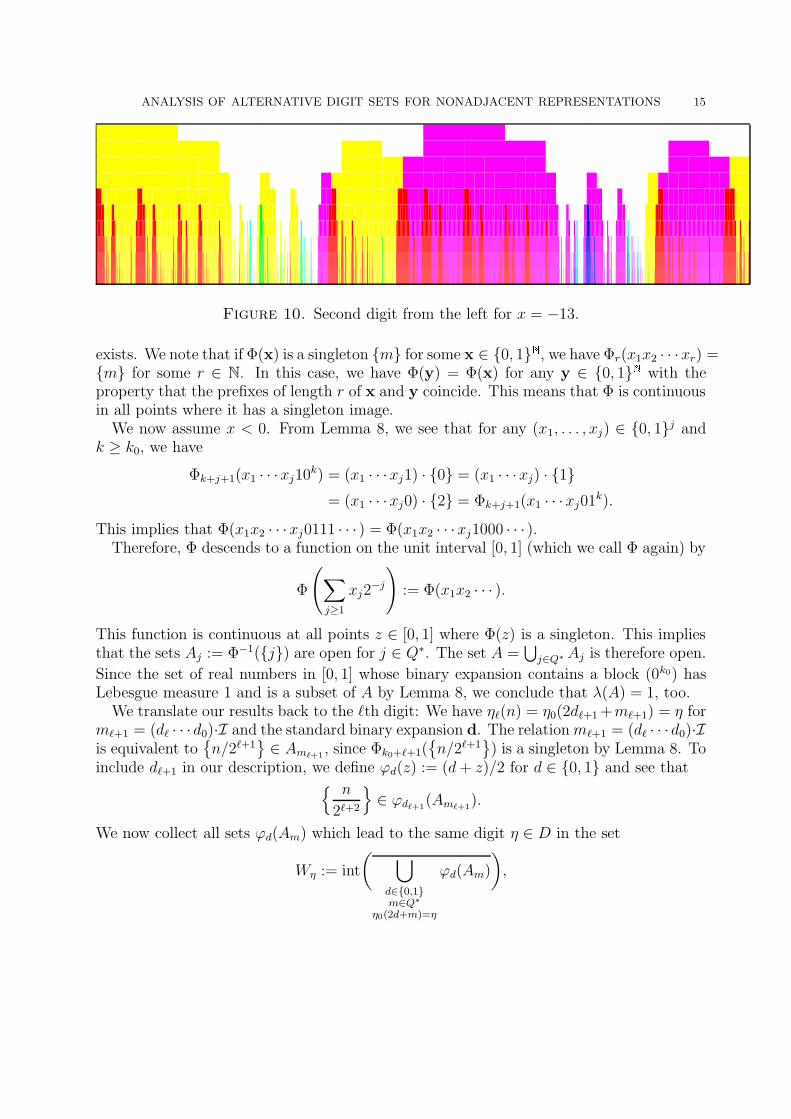
denotes the fractional part of z.In Figures 7, 8, 9, and 10, we draw the second digit from the left for x = 3, −1, −5, and
−13 respectively: For k = 3, . . . , 12 and n = 0, . . . , 2k − 1, we calculated the `th digit ofthe D-NAF of all integers m such that
n
2k≤{ m
2`+2
}<n + 1
2k;
these are those integers whose first (from the left!) digits in the standard binary expansionagree with the first digits of n. In some cases, the `th digit was the same for all integersm which lie in the given interval, in some cases, several digits could occur. We mappedthe sets of possible digits to colors according to Figure 6 and filled a rectangle of width1/2k and height 1 with this color at position (n/2k, 12− k). We remark that for x = −1,the picture is rather regular, whereas for x = −13, many decisions are still open after 12digits.
x 1
0
{1, x}
{0, 1}{0, x}D
Figure 6. Colors for Figures 7–10.
In what follows, we will describe this phenomenon in terms of the states of the transducerT .
Since the digit η` depends on the state m`+1 = (d` · · ·d0) · I and on d`+1, we will try topredict the state m`+1 from the knowledge of d` · · ·d`−r+1 for small r, wherever possible.Since we do not know in which state we are after reading the unknown digits d`−r · · ·d0,we have to assume that we are in any state (apart from the initial state). So we denotethe set Q \ {I} by Q∗.
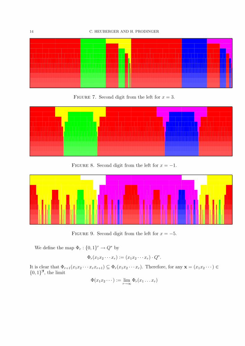
14 C. HEUBERGER AND H. PRODINGER
Figure 7. Second digit from the left for x = 3.
Figure 8. Second digit from the left for x = −1.
Figure 9. Second digit from the left for x = −5.
We define the map Φr : {0, 1}r → Q∗ by
Φr(x1x2 · · ·xr) := (x1x2 · · ·xr) ·Q∗.
It is clear that Φr+1(x1x2 · · ·xrxr+1) ⊆ Φr(x1x2 · · ·xr). Therefore, for any x = (x1x2 · · · ) ∈{0, 1}
�
, the limit
Φ(x1x2 · · · ) := limr→∞
Φr(x1 . . . xr)
ANALYSIS OF ALTERNATIVE DIGIT SETS FOR NONADJACENT REPRESENTATIONS 15
Figure 10. Second digit from the left for x = −13.
exists. We note that if Φ(x) is a singleton {m} for some x ∈ {0, 1}�
, we have Φr(x1x2 · · ·xr) ={m} for some r ∈ N. In this case, we have Φ(y) = Φ(x) for any y ∈ {0, 1}
�
with theproperty that the prefixes of length r of x and y coincide. This means that Φ is continuousin all points where it has a singleton image.
We now assume x < 0. From Lemma 8, we see that for any (x1, . . . , xj) ∈ {0, 1}j andk ≥ k0, we have
Φk+j+1(x1 · · ·xj10k) = (x1 · · ·xj1) · {0} = (x1 · · ·xj) · {1}= (x1 · · ·xj0) · {2} = Φk+j+1(x1 · · ·xj01k).
This implies that Φ(x1x2 · · ·xj0111 · · · ) = Φ(x1x2 · · ·xj1000 · · · ).Therefore, Φ descends to a function on the unit interval [0, 1] (which we call Φ again) by
Φ
(∑
j≥1
xj2−j
):= Φ(x1x2 · · · ).
This function is continuous at all points z ∈ [0, 1] where Φ(z) is a singleton. This impliesthat the sets Aj := Φ−1({j}) are open for j ∈ Q∗. The set A =
⋃j∈Q∗ Aj is therefore open.
Since the set of real numbers in [0, 1] whose binary expansion contains a block (0k0) hasLebesgue measure 1 and is a subset of A by Lemma 8, we conclude that λ(A) = 1, too.
We translate our results back to the `th digit: We have η`(n) = η0(2d`+1 +m`+1) = η form`+1 = (d` · · ·d0)·I and the standard binary expansion d. The relationm`+1 = (d` · · ·d0)·Iis equivalent to
{n/2`+1
}∈ Am`+1
, since Φk0+`+1({n/2`+1
}) is a singleton by Lemma 8. To
include d`+1 in our description, we define ϕd(z) := (d+ z)/2 for d ∈ {0, 1} and see that{ n
2`+2
}∈ ϕd`+1
(Am`+1).
We now collect all sets ϕd(Am) which lead to the same digit η ∈ D in the set
Wη := int
( ⋃
d∈{0,1}m∈Q∗
η0(2d+m)=η
ϕd(Am)
),

16 C. HEUBERGER AND H. PRODINGER
where the bar denotes closure and int denotes the interior. We take the interior of theclosure for “aesthetical reasons”: We want to avoid “holes” in the sets which would onlybe meaningful at the level of the transducer, but not on the level of the digits. Since{n/2`+1
}is in the interior of some Am anyway, the dyadic points are not affected by this
operation.This yields the following theorem.
Theorem 10. Let D = {0, 1, x} be a NADS with x < 0. There are disjoint open subsetsWη, η ∈ D, of the unit interval [0, 1] such that
η`(n) = η ⇐⇒{n/2`+2
}∈ Wη
for ` ≥ 0. The sum of the Lebesgue measures of the Wη, η ∈ D, equals 1.
6. Dimension of the boundary
Theorem 10 shows that
[0, 1] \ (W0 ∪W1 ∪Wx) = ∂(W0 ∪W1 ∪Wx) = ∂W0 ∪ ∂W1 ∪ ∂Wx
has Lebesgue measure zero. However, Figures 9 and 10 demonstrate that this “exceptionalset” is quite “irregular.” The aim of this section is to quantify this “irregularity” in termsof Hausdorff dimension.
We will calculate the Hausdorff dimension of ∂(W0 ∪W1 ∪Wx) as the spectral radius ofthe adjacency matrix of an auxiliary automaton as follows.
We construct auxiliary automata Am for m ≥ 2. The set of states is the set Qm :={I ⊆ Q∗ : #I = m} of m element subsets of Q∗. The alphabet is still {0, 1}. The set oftransitions
Em := {I d−→ J : J = d · I = {d · i : i ∈ I}, d ∈ {0, 1}, I, J ∈ Qm}is defined in terms of the transitions in the input automaton underlying T . All statesare initial and terminal states. The adjacency matrix of Am will be denoted by Mm. Forx = −5 and m = 2, this automaton is shown in Figure 11.
We will mainly work with A2, which is the only automaton to occur in the statement ofour result, however in some cases, we may be forced to use Am for some m > 2 instead.
The remaining part of this section is devoted to the proof of the following theorem.
Theorem 11. Let D = {0, 1, x} with x < 0 be a NADS and Wη, η ∈ D, be the setsdescribed in Theorem 10. Let ρ(M2) denote the spectral radius of the adjacency matrix M2
of A2. Then we havedimH(∂(W0 ∪W1 ∪Wx)) = log2 ρ(M2)
and0 < Hlog2 ρ(M2)(∂(W0 ∪W1 ∪Wx)) <∞.
For x = −1, we have log2 ρ(M2) = 0, for |x| ≥ 5, we have
0 < 0.347121− 1.04136
`+ 2≤ log2 ρ(M2) ≤ 1− 1
2k0 log 2+
1
22k0+1 log 2< 1,

ANALYSIS OF ALTERNATIVE DIGIT SETS FOR NONADJACENT REPRESENTATIONS 17
0, 1 0, 4
0, 2
0, 3
1, 4
1, 2
1, 34, 24, 3
2, 3
1
0
1
0 1
01
0
1
0
1 0
1
0
1
0
1
0
Figure 11. Automaton A2 for x = −5.
where k0 has been defined in (3.3) and ` = blog2(|x|+ 3)c − 1.For |x| ≤ 29, the values log2 ρ(M2) are shown in Table 2.
The transitions in Am will again be denoted by J = d · I, since this coincides with theearlier definition for subsets of Q∗. However, this transition is not defined in Am for everyd and I, since it might be the case that I is mapped to some J with #J < m. We willalso reuse the notation d · I for strings d ∈ {0, 1}n.
As in the previous section, we first study the problem at the level of the states of thetransducer and will translate them back to the level of output digits afterwards. Weconsider the set B := [0, 1]\A of those real numbers which do not allow us to decide aboutthe final state from the knowledge of a finite number of digits. To calculate the Hausdorffdimension of B for general x, we proceed as follows: We first derive an upper bound forthe box dimension using a suitable covering of B. In a second step, we construct a lowerbound for the box dimension. Finally we will show that a subset of B can be interpretedas a finite union of graph directed sets (cf. Falconer [4]) satisfying an open set condition,which implies (cf. Edgar [3]) that the Hausdorff, box and similarity dimensions are equal.Finally, we use this fact for calculating the Hausdorff Dimension of B explicitly for smallvalues of |x|.

18 C. HEUBERGER AND H. PRODINGER
x #Q #Q2 r(A2) dimH(∂(W0 ∪W1 ∪Wx))−1 3 3 2 0−5 5 10 3 0.7618−13 9 36 7 0.9003−17 10 45 6 0.9037−25 14 91 17 0.9364−29 14 91 8 0.9357−37 18 153 34 0.9492−53 22 231 25 0.9606−61 25 300 55 0.9547−65 25 300 33 0.9477−113 37 666 79 0.9733−121 41 820 147 0.9729−125 39 741 83 0.9649−137 42 861 98 0.9757−145 48 1128 228 0.9763−149 46 1035 130 0.9790
Table 2. Order of T and of A2, number r(A2) of strongly connected com-ponents of A2, and Hausdorff dimension of ∂(W0 ∪W1 ∪Wx).
So we start by giving an upper bound for the upper box dimension
dimBB = lim supn→∞
log2N2−n(B)
n,
where N2−n(B) denotes the number of 2−n-mesh intervals that intersect B. We have
(6.1) N2−n(B) = #{d ∈ {0, 1}n : Φn(d) is not a singleton},since if Φn(d) is not a singleton, there are two points z1 and z2 in the interval [
∑j dj2
−j,∑
j dj2−j+
2−n] lying in disjoint open sets Am1and Am2
. Therefore, there must be a point of B betweenz1 and z2.
Lemma 12. For k0 defined in (3.3), we have
(6.2) dimB(B) ≤ 1− 1
2k0 log 2+
1
22k0+1 log 2.
Proof. By Lemma 8, we have N2−n(B) ≤ #Un, where
Un ={(x1, . . . , xn) ∈ {0, 1}n : (xj, . . . , xj+k0−1) /∈ {(0k0), (1k0)} for all 1 ≤ j ≤ n− k0 +1
}.
The strings in Un can be described by a regular expression
(ε+ 0 + · · ·+ 0k0−1)((1 + 12 + · · ·+ 1k0−1)(0 + 02 + · · ·+ 0k0−1)
)∗(ε+ 1 + · · ·+ 1k0−1),

ANALYSIS OF ALTERNATIVE DIGIT SETS FOR NONADJACENT REPRESENTATIONS 19
which can be translated to the generating function
G(z) :=∑
n≥0
#Unzn
= (1 + · · ·+ zk0−1) · 1
1− (z + · · ·+ zk0−1)2· (1 + · · ·+ zk0−1) =
1− zk0
1− 2z + zk0.
Let q(z) := 1− 2z + zk0 . We note that we have k0 ≥ 4 by (3.3). Then |q(z)− (1− 2z)| =|zk0 | < 2 |z| − 1 ≤ |1− 2z| for 1− δ < |z| < 1 for a suitable δ. Therefore, q(z) has exactlyone zero with modulus less than 1, say ρ, by Rouche’s Theorem. Since q(1/2) > 0 andq(1/2 + 1/(2k0)) < 0, we know that ρ is real and ρ = 1/2 + O(k0
−1). By bootstrapping,we obtain
ρ =1 + ρk0
2=
1
2+O(2−k0), ρ =
1
2+
1
2k0+1+O
(k0
4k0
).
In fact, we have
(6.3) ρ ≥ 1
2+
1
2k0+1
for k0 ≥ 4, since q(2−1 + 2−(k0+1)) > 0.Defining the constant
ck0:= lim
z→ρG(z)
(1− z
ρ
),
we have#Un = [zn]G(z) =
ck0
ρn+O(1).
Therefore, we conclude that the upper box dimension of B can be bounded from above bydimB(B) ≤ − log2 ρ, hence (6.3) yields (6.2). �
We now derive lower bounds for the box dimension.
Lemma 13. Let |x| ≥ 5. Then we have(6.4)
dimB(B) = lim infn→∞
log2N2−n(B)
n≥(
1
2− 3
2`+ 4
)log2
1 +√
5
2≈ 0.347121− 1.04136
`+ 2> 0,
where ` = blog2(|x|+ 3)c − 1.
Proof. From the definition of T , we deduce that 0 and 1 always have the neighbourhoodshown in Figure 12, where s := (3 + |x|)/2. We further notice that any path from s to 1has at least length ` = blog2 sc, since m ≥ 2i implies r(2d+m) ≥ 2i−1 for d ∈ {0, 1}. Weconsider the set of sequences
(6.5) Ln := {d = (dn, . . . , d1) ∈ {0, 1}n : didi+1 = 0 for 1 ≤ i < n
and if (di · · ·d1) · s = 1 then di+1 = 1 for 1 ≤ i < n}.We claim that d · s 6= d · 0 for all d ∈ Ln. To prove this, we observe that d · 0 = dn. Forany 1 ≤ i ≤ n, we have (di · · ·d1) · s ≥ 1 by definition (and the known neighbourhood of 0

20 C. HEUBERGER AND H. PRODINGER
I
0 1
s
2
other states
0|ε
1|ε
0|0
1|00|1
1|x
0|0
1|0
Figure 12. Structure of T for general x (Neighbourhoud of I, 0, 1 is correct.)
and 1). If (di · · ·d1) · s = 1, we have di = 0, which implies (di · · ·d1) · 0 = 0. This provesthe claim. By (6.1), this implies that N2−n(B) ≥ #Ln.
We now derive a lower bound for #Ln. For 1 ≤ t ≤ ` we have
Lt := {(dt, . . . , d1) ∈ {0, 1}t : didi+1 = 0 for 1 ≤ i < t},since the second condition is no restriction for sequences of that length. The regularexpression for sequences which avoid adjacent 1s is 0∗(100∗)∗(ε + 1), the correspondinggenerating function equals
1
1− z1
1− z2
1−z
(1 + z) =1 + z
1− z − z2=∑
t≥0
Ft+2zt,
where Ft denotes the Fibonacci sequence Ft+2 = Ft+1 + Ft with F0 = 0 and F1 = 1.Therefore, we get
#Lt = Ft+2 =αt+2
√5− O(α−t) ≥ αt.
for α = (1 +√
5)/2 and 1 ≤ t ≤ `. For d = (d`−2, . . . , d0) ∈ L`−1 we define
ψ(d) := 1h((d0) · s)d0,
where h(m) is the input label of a shortest path from state m to state 1 whose input labeldoes not start (at the right) with 1 and does not contain adjacent ones. We note that if(d0) · s = 1, we have d`−2 = 0, h(1) = ε, and ψ(d) does not contain adjacent ones.

ANALYSIS OF ALTERNATIVE DIGIT SETS FOR NONADJACENT REPRESENTATIONS 21
If m 6= 0, we write h(m) = h′(0 ·m), where h′(m′) is the input label of a shortest pathfrom state m′ to state 1 whose input label does not contain adjacent ones. We claim that
(6.6) blog2m′c ≤ |h′(m′)| ≤ blog2m
′c+ 1,
where |h′(m′)| denotes the length of h′(m′). The left inequality follows from the argumentgiven before (6.5). For the right inequality, we choose the input digit d to be 0 unlessm′ ≡ 3 (mod 4), in which case we take d = 1. Thus η0(2d+m′) ∈ {0, 1} and r(2d+m′) =d+bm′/2c. If we choose d = 1, it is clear that r(2d+m′) is even so that we will not chooseinput 1 in the next step. Furthermore, we have blog2(r(2d+m′))c = blog2(m
′)c− 1 unlessm′ = 2g−1 for some g. But in the latter case, we have r(2d+m′) = 2g−1 with |h′(m′)| = g.Therefore, (6.6) follows by induction.
We conclude that
|h′(m′)| ≤ blog2m′c + 1 ≤ blog2(|x|+ 2)c+ 1 ≤ `+ 2
and therefore |ψ(d)| ≤ 2`+ 4. We now define an injective map Lbn/(2`+4)c`−1 → Ln by
(dbn/(2`+4)c, . . . ,d1) 7→ d0
(n−
bn/(2`+4)c∑
j=1
|ψ(dj)|)ψ(dbn/(2`+4)c) · · ·ψ(d1),
where d0(m) ∈ Lm is some fixed admissible string of length m which is used to obtain therequired length n. This yields
#Ln ≥ α(`−1)bn/(2`+4)c ≥ 1
α`−1·(α(`−1)/(2`+4)
)n.
For |x| ≥ 5, the bound (6.4) follows. �
We want to prove that the lower box, upper box, Hausdorff and similarity dimensionsof B agree. To this aim, we first collect a few simple consequences of Perron-Frobeniustheory.
We denote the spectral radius of a (n× n)-matrix M by ρ(M). If I, J ⊆ {1, . . . , n}, wedenote the submatrix of M with rows I and columns J by M(I, J).
If M = (mij)1≤i,j≤n is a nonnegative (n × n)-matrix, we will consider the digraph Ginduced by M , i.e., the directed graph with set of vertices {1, . . . , n} and set of arcs{(i, j) : mij > 0}. We will call any strongly connected component C ⊆ {1, . . . , n} of Gwhich fulfills
(6.7) ρ(M(C, C)) = ρ(M)
a dominating component of M . We will identify subsets of {1, . . . , n} and the subgraph ofG induced by these vertices when speaking about strongly connected components.
Lemma 14. Let M be a nonnegative (n× n)-matrix. Then there is a nonnegative vector0 6= x ∈ R
n such that
Mx = ρ(M)x.
Let G be the directed graph induced by M . Then M has a dominating component.

22 C. HEUBERGER AND H. PRODINGER
Proof. By continuity, the assertion on the nonnegative eigenvector follows from the Perron-Frobenius theorem, cf. [11, Theorem 15.5.1], for instance.
Let C1, . . . , Cr be the strongly connected components of G. We consider the auxiliarydigraph G′ with set of vertices {C1, . . . , Cr} and an arc from Ci to Cj if there is an arc fromsome vertex in Ci to some vertex in Cj in the original digraph G. By construction, theauxiliary digraph G′ has no directed cycle. This implies that we may sort the componentsin such a way that the adjacency matrix of G′ is upper triagonal. If we permute the rowsand columns of M according to the strongly connected components, we get a matrix whichis block upper triagonal. Therefore, the spectrum σ(M) of M equals
σ(M) =
r⋃
i=1
σ(M(Ci, Ci)).
This implies that ρ(M) = maxi=1,...,r ρ(M(Ci, Ci)). This proves the existence of a dominat-ing component. �
Lemma 15. Let M be a nonnegative (n× n)-matrix and e = (1, . . . , 1)t ∈ Rn. Then
limm→∞
log2(etMme)
m= log2 ρ(M),
which may equal −∞.
Proof. Each entry of Mm is bounded by a constant times mn−1ρ(M)m, so the same holdsfor the nonnegative number etMme.
On the other hand, let x be a nonnegative eigenvector of M for ρ(M), which exists byLemma 14. Without loss of generality, 0 ≤ xj ≤ 1 for j = 1, . . . , n. Therefore,
etMme ≥ xtMmx = ρ(M)mxtx.
Taking logarithms and limits yields the result. �
In general, we cannot expect the automaton Am to be strongly connected. Therefore,we cannot apply the results on graph directed sets directly, but we have to apply it onthe strongly connected components. To cover the remaining parts of B, we give an upperbound for the upper box dimension (and therefore for the Hausdorff dimension) using thespectral radius ρ(M2) of M2 at this point.
Lemma 16. We havedimH(B) ≤ dimB(B) ≤ log2 ρ(M2).
For |x| ≥ 5, we have ρ(M2) > 1.
Proof. Consider d ∈ {0, 1}n such that Φn(d) is not a singleton. Then there are u 6= v ∈ Q∗
such that d · u 6= d · v, i.e., there is at least one path in A2 from some {u, v} ∈ Q2 to some{u′, v′} ∈ Q2 with label d. Thus the number N2−n(B) can be bounded from above by thenumber of paths of length n in A2, which equals etMn
2 e. From Lemma 15 we conclude that
dimB(B) = lim supn→∞
log2N2−n(B)
n≤ lim sup
n→∞
log2 etMn
2 e
n= log2 ρ(M2).

ANALYSIS OF ALTERNATIVE DIGIT SETS FOR NONADJACENT REPRESENTATIONS 23
It is well known that the Hausdorff dimension is always less or equal the lower (and thereforethe upper) box dimension.
Since dimB(B) > 0 for |x| ≥ 5 by Lemma 13, we conclude that ρ(M2) > 1 in thatcase. �
Proof of Theorem 11. We assume that |x| ≥ 5.Since 0 /∈ 1 · Q∗ (cf. Figure 12), the automaton A#Q∗ has one state and at most one
transition, hence ρ(M#Q∗) ≤ 1 < ρ(M2) by Lemma 16. We now choose m ≥ 2 maximalsuch that ρ(Mm) ≥ ρ(M2). The preceeding observation implies that m < #Q∗.
We define sets VI := {x ∈ [0, 1] : I ⊆ Φ(x)} for I ∈ Qm. By definition of Φ, these setsare compact. We consider the contracting similarities ϕd(z) := (d + z)/2 for d ∈ {0, 1}.We clearly have Φ(ϕd(z)) = d · Φ(z) for d ∈ {0, 1} and z ∈ [0, 1]. Then it is easily provedthat
(6.8) VI =⋃
d∈{0,1}J∈Qm
I=d·J
ϕd(VJ), I ∈ Qm.
Let now C ⊆ Qm be a dominant component of Mm, i.e., ρ(Mm(C, C)) ≥ ρ(M2) > 1.First, we claim that
(6.9) VI 6= ∅ for every I ∈ C.To this aim, we note that there is a directed cycle I
d−→ I in C, where d ∈ {0, 1}r for some1 ≤ r ≤ #C. It follows that
Φsr(ds) = ds ·Q∗ ⊇ ds · I = I,
which implies that Φ(dω) ⊇ I, where dω denotes the infinite word ddd · · · . The realnumber z with binary expansion 0.ddd · · · is therefore an element of VI. This proves (6.9).
Next, we claim that
(6.10) UI := {z ∈ [0, 1] : I = Φ(z)} 6= ∅ for every I ∈ C.To prove this, we assume that UI = ∅ for some I ∈ C. Let now d ∈ {0, 1}n for some n ∈ N
be the label of a path of length n in C, i.e., there are K1, K2 ∈ C such that K1d−→ K2 is a
path in C. We take some z ∈ VK1and a path K2
d′
−→ I in C. We have
Φ(ϕd′d(z)) = d′d · Φ(z) ⊇ d′d ·K1 = I,
where ϕ � is defined by ϕδ1···δn:= ϕδ1 ◦ · · · ◦ ϕδn
.Since UI = ∅ by assumption, this implies that
# (d ·Q∗) ≥ # (d′d ·Q∗) ≥ #Φ(ϕd′d(z)) > #I = m,
which yields # (d ·Q∗) ≥ m+ 1. This means that there is a path K3d−→ K4 of length n in
Am+1. The above construction shows that there is an injective map from the set of labelsof paths of length n in C to the set of paths of length n in Am+1. We obtain
etMnm+1e ≥ #{d ∈ {0, 1}n : d is label of a path of length n in C} ≥ 1
#C2etMm(C, C)ne.

24 C. HEUBERGER AND H. PRODINGER
By Lemma 15, we conclude that
log2 ρ(Mm+1) = limn→∞
log2(etMn
m+1e)
n
≥ limn→∞
log2
(1
#C2 etMm(C, C)ne
)
n= log2 ρ(Mm(C, C)) = log2(ρ(M2)).
This yields ρ(Mm+1) ≥ ρ(M2), a contradiction to the choice of m. Hence our claim (6.10)is proved.
We now restrict (6.8) to the component C: There is a unique collection of nonemptycompact sets (V C
I )I∈C, such that
(6.11) V CI =
⋃
d∈{0,1}J∈C
I=d·J
ϕd(VCJ ), I ∈ C,
cf. for instance Edgar [3, Theorem 4.3.5]. These sets V CI , I ∈ Qm, are the graph directed
sets defined by C and the contractions ϕd, cf. Falconer [4].It is clear that V C
I ⊆ VI for each I ∈ C, since the fixed point (V CI )I∈C of (6.11) can
be obtained by iterating the right hand side of (6.11) starting with the collection (VI)I∈C,which yields a sequence of tuples of compact sets which is nonincreasing in each componentby (6.8).
For I ∈ C, we define
OI := {z ∈ [0, 1] : d(z, VI) < d(z, VJ) for all J ∈ Qm ∪ {∂} with J 6= I},where V∂ := {0, 1} is the boundary of the unit interval, d(z,K) := inf{d(z, y) : y ∈ K} forcompact sets K and the Euclidean distance d(z, y). The sets OI , I ∈ C, are open. SinceΦ(0) = {0} and Φ(1) = {2} by Lemma 8, we have UI ⊆ OI , hence OI 6= ∅ for I ∈ C by(6.10). It is easily checked that for fixed I ∈ C, we have
(6.12)ϕd(OJ) ⊆ OI, for all d ∈ {0, 1}, J ∈ C with I = d · J,
the sets ϕd(OJ) for d ∈ {0, 1}, J ∈ C with I = d · J are disjoint.
This is the open set condition, cf. Edgar [3, Definition 6.4.7].Therefore, by Edgar [3, Theorem 6.4.8], we have dimH(V C
I ) = s and Hs(V CI ) > 0 for all
I ∈ C, where s is the unique similarity dimension such that ρ(2−sMm(C, C)) = 1. Thus wehave s = log2 ρ(Mm). Since V C
I ⊆ VI ⊆ B and
0 < Hlog2 ρ(Mm)(V CI ) ≤ Hlog2 ρ(Mm)(B) ≤ Hlog2 ρ(M2)(B) <∞
by definition of m and Lemma 16, we have dimH(B) = dimB(B) = log2 ρ(M2).Finally, we translate this result to the sets Wη defined in Theorem 10. From the definition
of Wη we conclude that for η ∈ {0, 1, x}, we have
(6.13) Hlog2 ρ(M2)(∂Wη) ≤∑
d∈{0,1}m∈Q∗
η0(2d+m)=η
1
ρ(M2)Hlog2 ρ(M2)(∂Am) <∞.

ANALYSIS OF ALTERNATIVE DIGIT SETS FOR NONADJACENT REPRESENTATIONS 25
We now choose I ∈ C and {u, v} ⊆ I in such a way that u 6= v and v2(u− v) is minimal,where v2(n) denotes the maximal t such that 2t divides n. Since ρ(M2) > 1 by Lemma 16,there is a transition J = d·I in C. We set u′ = d·u and v′ = d·v. As #I = #J = m, we haveu′ 6= v′. If u ≡ v (mod 4), then u′−v′ = 1/2(u−η0(2d+u))−1/2(v−η0(2d+v)) = 1/2(u−v),so v2(u
′ − v′) < v2(u − v), a contradiction. If u and v are both even, we similarly getu′−v′ = 1/2(u−v), which is also a contradiction. Therefore, we have η0(2d+u) 6= η0(2d+v).Let now z ∈ VI . By definition of Φ, every neighborhood of z contains a point z1 ∈ Au anda point z2 ∈ Av. We clearly have ϕd(z1) ∈ Wη0(2d+u) and ϕd(z2) ∈ Wη0(2d+v), which impliesthat ϕd(z) ∈ ∂(W0 ∪W1 ∪Wx). We conclude that
(6.14) 0 <1
ρ(M2)Hlog2 ρ(M2)(V C
I ) = Hlog2 ρ(M2)(ϕd(VCI )) ≤ Hlog2 ρ(M2)(∂(W0 ∪W1 ∪Wx)).
This concludes the proof of the theorem for |x| ≥ 5.For x = −1, we note that ρ(M2) = 1, which implies that dimH(∂(W0 ∪W1 ∪Wx)) = 0
by Lemma 16. It can easily be checked that in this case, we have
W0 = [0, 1/6) ∪ (2/6, 4/6) ∪ (5/6, 1],
W1 = (1/6, 2/6),
W−1 = (4/6, 5/6),
and therefore H0(∂(W0 ∪W1 ∪Wx)) = 4.The remaining dimensions in Table 2 have been computed using Mathematica r©. �
7. Geometric Approach for Calculating the Frequency of Digits
We give a geometric approach (going back to Delange [2]) using the results in the pre-ceeding sections to compute the summatory function of the frequency of digits. In contrastto the results in Section 4, we are now able to compute the summatory function up tosome integer N instead of considering the full block length {0, . . . , 2L− 1} as in Section 4.However, we will need the results of that section to compute the Lebesgue measures of thesets Wd, d ∈ {0, 1, x}.
For d ∈ {1, x} and positive N ∈ Z, let
Hd(N) :=
N−1∑
n=0
fd(n) =
N−1∑
n=0
∑
k≥0
[ηk(n) = d] ,
where fd(n) has already been defined in (4.1). Since ηk(n) = 0 for k > blog2(n)c+ #Q− 2by Theorem 7, Theorem 10 implies that
Hd(N) =N−1∑
n=0
K+1∑
k=0
[{ n
2k+2
}∈ Wd
],
where K = blog2Nc + #Q − 2. We proceed as in Section 4 of [5]: We replace Wd byan appropriate approximation Wd,k, replace the sum by an integral and pull out the main

26 C. HEUBERGER AND H. PRODINGER
term given by the Lebesgue measure of Wd. Since the technical modifications are straightforward, we skip the details. We get
(7.1) Hd(N) = λ(Wd)N log2N +Nψd({log2 N}) +O(N log2 ρ(M2)),
where ρ(M2) is the dominant eigenvalue of the auxiliary automaton as in Theorem 11,
ψd(z) := λ(Wd)(#Q− {z}) + 2{z}+#Q−2Ψd(2{z}+2−#Q) +
∞∑
k=−1
βk,
Ψd(t) :=∞∑
k=0
∫ t
0
([{x2k−2
}∈ Wd
]− λ(Wd)
)dx,
βk :=
∫ 1
0
([{x} ∈ Wd,k]− [{x} ∈ Wd]
)dx,
Wd,k :=⋃
m∈2k+2Wd∩ �
[m
2k+2,m+ 1
2k+2
).
As in [5] we see that ψd(z) is continous in [0, 1) and that limz→1− ψd(z) exists. Of course,ψd is 1-periodic. We cannot conclude that ψd is continuous at z = 1 by direct computationas in [5]. Instead, we get continuity by considering
O(L) = Hd(2L)−Hd(2
L − 1) = 2L(ψd(0)− ψd
({log2
(1− 1
2L
)}))+O(L).
Comparing with Theorem 9, we see that (7.1) implies that λ(Wd) = 1/6 for d ∈ {1, x}.Since λ(W0 ∪W1 ∪Wx) = 1 we must have λ(W0) = 2/3.
We summarize this result in the following theorem.
Theorem 17. Let D = {0, 1, x} be a NADS, d ∈ {1, x} and N be a positive integer. Thenthe number of occurrences of the digit d in the D-NAFS of the integers 0, . . . , N−1 equals
Hd(N) =1
6N log2N +Nψd({log2N}) +O(N log2 ρ(M2)),
where ψd is a 1-periodic continuous function and ρ(M2) < 2 is the spectral radius of theadjacency matrix of the auxiliary automaton described in Section 6.
Moreover, the Lebesgue measures of the sets Wd described in Theorem 10 equal
λ(W1) = λ(Wx) =1
6, λ(W0) =
2
3.
8. Non-Optimality
ForD = {0, 1,−1}, theD-NAF of n has minimal Hamming weight amongst all {0, 1,−1}-expansions of n, cf. Reitwiesner [15], where the Hamming weight c(η) of an expansionη ∈ D
�0 equals the number of nonzero digits #{j : ηj 6= 0}.
For x ≤ −5, this is no longer the case:
Theorem 18. Let D = {0, 1, x} be a NADS. Then the following two conditions are equiv-alent:

ANALYSIS OF ALTERNATIVE DIGIT SETS FOR NONADJACENT REPRESENTATIONS 27
• For every positive integer n, the Hamming weight of the D-NAF of n is minimumamongst all D-expansions of n.• x ∈ {−1, 3}.
We first consider the case x = 3 and give an algorithmic proof, which can also be usedin more general situations. For instance, the case x = −1 follows along the same lines.
Lemma 19. The {0, 1, 3}-NAF is the {0, 1, 3}-expansion of minimal Hamming weight.
Proof of the lemma. We consider the transducer T (cf. Figure 13). We introduce weights
I0
1
3
2
4 5
0|ε
1|ε3|ε
0|0
1|0
3|0
0|1, 1|33|3
0|31|1
3|1
0|01|0
3|01|0
0|03|0
0|1, 1|3
3|3
Figure 13. Transducer T calculating a {0, 1, 3}-NAF of n from any{0, 1, 3}-expansion of n from right to left.
for the transitions:
w(id|o−→ j) := c(d)− c(o),
where c denotes the Hamming weight and c(ε) = 0. If we have a successful path I d| �−−→ 0,the weight of this path equals c(d)− c(η). We calculate the shortest path from I to 0 inthis weighted digraph using the Ford-Bellman algorithm (cf. Cook et al. [1]). It turns outthat the shortest path has weight 0, i.e. c(d)− c(η) ≥ 0, as requested. �
Remark 20. We note that the above proof of Lemma 19 also yields a complete descriptionof all {0, 1, 3}-expansions of minimal weight: The Ford-Bellman algorithm calculates afeasible potential π : V → Z, where π(i) is the weight of a shortest path from I to i. Inour case, we have
i I 0 1 2 3 4 5,π(i) 0 0 1 1 1 1 2.
Thus if we have π(i) + w(id|o−→ j) > π(j) for some transition, the transition corresponds
to an actual gain when modifying the given representation d to the D-NAF. Therefore,

28 C. HEUBERGER AND H. PRODINGER
we remove all those transitions and all output labels and get an automaton which acceptsminimal {0, 1, 3}-expansions, see Figure 14. In this figure, we also identified states 0 andI, since they only differed in the output labels of the transitions leaving them.
0
1
3
2
4 5
0
1
3
03
0
1
3
0
0
3
0
Figure 14. Automaton accepting all binary {0, 1, 3}-expansions of minimalHamming weight.
If we use the same approach for x = −1, we get the transducer in Figure 15 and theautomaton in Figure 16, respectively. The transducer corresponds to the algorithm due toJedwab and Mitchell [9], the automaton to the syntactical rules described in Heuberger [?].
Proof of Theorem 18. By Lemma 19 and Reitwiesner [15], we only have to consider thecase x ≤ −5. If |x|+ 3 = 2g for some g ≥ 4, we consider n = 2g+1 + 7. We have
n = 1 · 22g + x · 2g + 1 · 22 + x · 20,(8.1)
n = 1 · 2g+2 + x · 2 + 1.(8.2)
Both are {0, 1, x}-expansions, (8.1) is the D-NAF with Hamming weight 4, whereas (8.2)is an expansion of Hamming weight 3.
If x = −5, we have
23 = value(10050505),(8.3)
23 = value( 100051).(8.4)
The first expansion (8.3) is the D-NAF, again with Hamming weight 4, the second expan-sion has Hamming weight 3.
Next, if |x|+3 is not a power of 2, we consider n = 3. We have η0(3) = x, η1(3) = 0 andr2(3) = (3+ |x|)/4. By assumption, (3+ |x|)/4 is not a power of 2. Since (3+ |x|)/4 < |x|,we conclude that any D-expansion of (3+ |x|)/4 has Hamming weight at least 2, therefore,

ANALYSIS OF ALTERNATIVE DIGIT SETS FOR NONADJACENT REPRESENTATIONS 29
I0
1
−1
2
−2
0|ε
1|ε1|ε
0|0
1|0
1|0
0|1, 1|1
1|1
0|1, 1|1
1|1
1|0
0|01|0
1|0
0|01|0
Figure 15. Transducer T calculating a {0, 1,−1}-NAF of n from any{0, 1,−1}-expansion of n from right to left.
0
1
−1
2
−20
1
1
0
1
0
1
0
0
Figure 16. Automaton accepting all binary {0, 1,−1}-expansions of mini-mal Hamming weight.
the D-NAF of 3 has Hamming weight at least 3. However, the standard binary expansion3 = value(11) has lower Hamming weight. �
9. Addition of 1
The transducer for calculating the addition of 1 for x = −5 is shown in Figure 17.
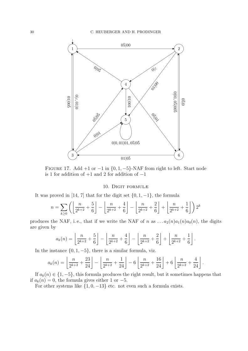
30 C. HEUBERGER AND H. PRODINGER
1 2
3
4
5
6
05|00
0|ε,0
1|0
0|ε
01|00
05|0
01|0
05
05|05
0|01
0|05
01|0
01
05|01
0|0, 01|01, 05|05
0|01,0
5|005
01|05
Figure 17. Add +1 or −1 in {0, 1,−5}-NAF from right to left. Start nodeis 1 for addition of +1 and 2 for addition of −1
10. Digit formulæ
It was proved in [14, 7] that for the digit set {0, 1,−1}, the formula
n =∑
k≥0
(⌊n
2k+2+
5
6
⌋−⌊
n
2k+2+
4
6
⌋−⌊
n
2k+2+
2
6
⌋+
⌊n
2k+2+
1
6
⌋)2k
produces the NAF, i. e., that if we write the NAF of n as . . . a2(n)a1(n)a0(n), the digitsare given by
ak(n) =
⌊n
2k+2+
5
6
⌋−⌊
n
2k+2+
4
6
⌋−⌊
n
2k+2+
2
6
⌋+
⌊n
2k+2+
1
6
⌋.
In the instance {0, 1,−5}, there is a similar formula, viz.
ak(n) =
⌊n
2k+2+
23
24
⌋−⌊
n
2k+2+
1
24
⌋− 6
⌊n
2k+2+
16
24
⌋+ 6
⌊n
2k+2+
4
24
⌋.
If ak(n) ∈ {1,−5}, this formula produces the right result, but it sometimes happens thatif ak(n) = 0, the formula gives either 1 or −5.
For other systems like {1, 0,−13} etc. not even such a formula exists.

ANALYSIS OF ALTERNATIVE DIGIT SETS FOR NONADJACENT REPRESENTATIONS 31
References
1. W. J. Cook, W. H. Cunningham, W. R. Pulleyblank, and A. Schrijver, Combinatorial optimization,Wiley-Interscience Series in Discrete Mathematics and Optimization, John Wiley & Sons Inc., NewYork, 1998. MR 99b:90098
2. H. Delange, Sur la fonction sommatoire de la fonction“somme des chiffres”, Enseignement Math. (2)21 (1975), no. 1, 31–47. MR 52 #319
3. G. A. Edgar, Measure, topology, and fractal geometry, Undergraduate Texts in Mathematics, Springer-Verlag, New York, 1990. MR 92a:54001
4. K. Falconer, Techniques in fractal geometry, John Wiley & Sons Ltd., Chichester, 1997. MR 99f:280135. P. J. Grabner, C. Heuberger, and H. Prodinger, Distribution results for low-weight binary representa-
tions for pairs of integers, Theoret. Comput. Sci. 319 (2004), 307–331.6. R. L. Graham, D. E. Knuth, and O. Patashnik, Concrete mathematics. A foundation for computer
science, second ed., Addison-Wesley, 1994. MR 97d:680037. C. Heuberger and H. Prodinger, On minimal expansions in redundant number systems: Algorithms
and quantitative analysis, Computing 66 (2001), 377–393.8. H.-K. Hwang, On convergence rates in the central limit theorems for combinatorial structures, Euro-
pean J. Combin. 19 (1998), 329–343. MR 99c:600149. J. Jedwab and C. J. Mitchell, Minimum weight modified signed-digit representations and fast exponen-
tiation, Electron. Lett. 25 (1989), 1171–1172.10. D. E. Knuth, Seminumerical algorithms, third ed., The Art of Computer Programming, vol. 2, Addison-
Wesley, 1998.11. P. Lancaster and M. Tismenetsky, The theory of matrices, second ed., Computer Science and Applied
Mathematics, Academic Press Inc., Orlando, FL, 1985. MR 87a:1500112. J. A. Muir and D. R. Stinson, Alternative digit sets for nonadjacent representations, to appear in
Lecture Notes in Computer Science (Selected Areas in Cryptography, 2003), Preprint available athttp://www.cacr.math.uwaterloo.ca/~dstinson/papers/na_digitsets-pv.ps.
13. , Alternative digit sets for nonadjacent representations, Journal Version of [12]; Preprint avail-able at http://www.cacr.math.uwaterloo.ca/~dstinson/papers/na_digitsets-j.ps.
14. H. Prodinger, On binary representations of integers with digits −1, 0, 1, Integers 0 (2000), A08, avail-able at http://www.integers-ejcnt.org/vol0.html.
15. G. W. Reitwiesner, Binary arithmetic, Advances in computers, vol. 1, Academic Press, New York,1960, pp. 231–308.
(C. Heuberger) Institut fur Mathematik B, Technische Universitat Graz, Steyrergasse
30, 8010 Graz, Austria
E-mail address : [email protected]
(H. Prodinger) The John Knopfmacher Centre for Applicable Analysis and Number The-
ory, School of Mathematics, University of the Witwatersrand, P. O. Wits, 2050 Johan-
nesburg, South Africa
E-mail address : [email protected]