Analysis of a semigroup approach in the inverse problem of identifying an unknown coefficient

MATHEMATICAL METHODS IN THE APPLIED SCIENCESMath. Meth. Appl. Sci. 2008; 31:1635–1645Published online 5 February 2008 in Wiley InterScience(www.interscience.wiley.com) DOI: 10.1002/mma.989MOS subject classification: 35R 30; 47D 06; 39K 05

Analysis of a semigroup approach in the inverse problemof identifying an unknown coefficient

Ali Demir1 and Ebru Ozbilge2,∗,†

1Department of Mathematics, Kocaeli University, Umuttepe, 41380 Izmit-Kocaeli, Turkey2Department of Mathematics, Faculty of Science and Literature, Izmir University of Economics,

Sakarya Caddesi, No.156, 35330 Balcova-Izmir, Turkey

Communicated by W. Wendland

SUMMARY

This article presents a semigroup approach to the mathematical analysis of the inverse coefficient prob-lems of identifying the unknown coefficient k(ux ) in the quasi-linear parabolic equation ut (x, t)=(k(ux )ux (x, t))x +F(x, t), with Dirichlet boundary conditions u(0, t)=�0, u(1, t)=�1 and source func-tion F(x, t). The main purpose of this paper is to investigate the distinguishability of the input–outputmappings �[·] :K→C1[0,T ], �[·] :K→C1[0,T ] via semigroup theory. Copyright q 2008 John Wiley& Sons, Ltd.

KEY WORDS: semigroup approach; coefficient identification; parabolic equation

1. INTRODUCTION

Consider the following initial-boundary value problem:⎧⎪⎨⎪⎩ut (x, t)=(k(ux )ux (x, t))x +F(x, t), (x, t)∈�T

u(x,0)=g(x), 0<x<1

u(0, t)=�0, u(1, t)=�1, 0<t<T

(1)

∗Correspondence to: Ebru Ozbilge, Department of Mathematics, Faculty of Science and Literature, Izmir Universityof Economics, Sakarya Caddesi, No.156, 35330 Balcova-Izmir, Turkey.

†E-mail: [email protected]

Contract/grant sponsor: Scientific and Technical Research Council (TUBITAK) of TurkeyContract/grant sponsor: Izmir University of Economics

Copyright q 2008 John Wiley & Sons, Ltd. Received 8 June 2007

1636 A. DEMIR AND E. OZBILGE

where �T ={(x, t)∈ R2 :0<x<1,0<t�T }. The left and right boundary values �0,�1 are assumedto be constants. The functions c1>k(ux (x, t))�c0>0 and g(x) satisfy the following conditions:

(C1) |kux (u1x )−kux (u2x )|<d|u1x −u2x |;(C2) g(x)∈C2[0,1],g(0)=�0,g(1)=�1.

Under these conditions, the initial-boundary value problem (1) has the unique solution u(x, t)∈C2,1(�T )∩C2,0(�T ).

Consider the inverse problem of determining the unknown coefficient k=k(ux ) from oneor/and two Dirichlet and Neumann type of measured output data at the boundaries x=0 and 1,respectively:

ux (0, t)= f (t), ux (1, t)=h(t), t ∈(0,T ] (2)

where u=u(x, t) is the solution of the parabolic problem (1). The functions f (t),h(t) are assumedto be noisy-free measured output data. In this context, the parabolic problem (1) will be referredto as a direct ( forward) problem [1, 2], with the inputs g(x) and k(ux ). It is assumed that thefunctions f (t) and h(t) belong to C1[0,T ] and satisfy the consistency conditions f (0)=g′(0),h(0)=g′(1).

By denoting K :={k(ux ) :c1>k(ux (x, t))�c0>0, |kux (u1x )−kux (u2x )|<d|u1x −u2x |,u(x, t)∈C2,1(�T )∩C2,0(�T )}, the set of admissible coefficients k=k(ux ), introduce the input–outputmappings �[·] :K→C1[0,T ], �[·] :K→C1[0,T ], where

�[k]=ux (x, t;k)|x=0, �[k]=ux (x, t;k)|x=1, k∈K (3)

Then, the inverse problem with the measured output data f (t) and h(t) can be formulated as thefollowing operator equations:

�[k]= f, �[k]=h, k∈K, f,h∈C1[0,T ] (4)

The monotonicity, continuity, and hence, invertibility of the input–output mappings �[·] :K→C1[0,T ] and �[·] :K→C1[0,T ] are investigated in [3, 4] by using an adjoint problem approach.Moreover, the inverse coefficient problems for the quasi-linear parabolic equation are studied in[5, 6]. However, in this study the final data are taken as overspecified. In this paper, Dirichlet andNeumann type of measured output data at the boundaries x=0 and 1 are used in the identificationof the unknown coefficient. In addition to this, in the determination of the unknown coefficient,analytical results are obtained.

The purpose of this paper is to study the distinguishability of the unknown coefficient via theabove input–output mappings. We consider that the mapping �[·] :K→C1[0,T ] (or �[·] :K→C1[0,T ]) has the distinguishability property if �[k1] �=�[k2] (�[k1] �=�[k2]) implies k1(ux ) �=k2(ux ). This, in particular, means injectivity of the inverse mappings �−1 and �−1.

The paper is organized as follows. In Section 2, an analysis of the semigroup approach is givenfor the inverse problem, with the single measured output data f (t) given at the boundary x=0.In Section 3, a similar analysis is applied to the inverse problem with the single measured outputdata h(t) given at the point x=1. The inverse problem with two Neumann measured data f (t)and h(t) is discussed in Section 4. Some concluding remarks are given in Section 5.

Copyright q 2008 John Wiley & Sons, Ltd. Math. Meth. Appl. Sci. 2008; 31:1635–1645DOI: 10.1002/mma

ANALYSIS OF A SEMIGROUP APPROACH 1637

2. AN ANALYSIS OF THE INVERSE PROBLEM WITH GIVEN MEASURED DATA f (t)

Consider now the inverse problem with one measured output data f (t) at x=0. In order toformulate the solution of the parabolic problem (1) in terms of a semigroup, let the parabolicequation be arranged as follows:

ut (x, t)−(k(ux (0,0))ux (x, t))x =([k(ux )−k(ux (0,0))]ux (x, t))x +F(x, t), (x, t)∈�T

Hence, the initial-boundary value problem (1) can be rewritten in the following form:

ut (x, t)−k(ux (0,0))uxx (x, t) = ((k(ux )−k(ux (0,0)))ux (x, t))x +F(x, t), (x, t)∈�T

u(x,0) = g(x), 0<x<1

u(0, t) = �0, u(1, t)=�1, 0<t<T

(5)

For the time being we assume that k(ux (0,0)) is known; later this value will be determined.In order to formulate the solution of the parabolic problem (5) in terms of semigrouping, a newfunction needs to be defined:

v(x, t)=u(x, t)−�0(1−x)−�1x, x ∈[0,1] (6)

which satisfies the following parabolic problem:

vt (x, t)+A[v(x, t)] = ((k(vx (x, t)−�0+�1)−k(ux (0,0)))(vx (x, t)−�0+�1))x +F(x, t)

(x, t)∈�T

v(x,0) = g(x)−�0(1−x)−�1x, 0<x<1

v(0, t) = 0, v(1, t)=0, 0<t<T

(7)

Here, A[.] :=−k(ux (0,0))d2[.]/dx2 is a second-order differential operator and its domain is DA={v(x)∈C2(0,1)∩C1[0,1] :v(0)=v(1)=0}. Obviously g(x)∈DA, since the initial value functiong(x) belongs to C2[0,1].

Denote by T (t) the semigroup of linear operators generated by the operator −A [7, 8]. Notethat the eigenvalues and eigenfunctions of the differential operator A can easily be identified.Moreover, the semigroup T (t) can be constructed by using the eigenvalues and eigenfunctions ofthe infinitesimal generator A. Hence, the following eigenvalue problem must first be considered:

A�(x) = ��(x)

�(0) = 0, �(1)=0(8)

This problem is the Sturm–Liouville problem. The eigenvalues are determined as using �n =k(ux (0,0))n2�2 for all n=0,1, . . . , and the corresponding eigenfunctions are determined as using�n(x)=

√2sin(n�x). In this case, the semigroup T (t) can be represented in the following way:

T (t)U (x,s)=∞∑n=0

〈�n(�),U (�,s)〉e−�nt�n(x) (9)

where 〈�n(�),U (�,s)〉=∫ 10 �n(�)U (�,s)d�. The Sturm–Liouville problem (8) generates a

complete orthogonal family of eigenfunctions so that the null space of the semigroup T (t) is



trivial, i.e. N (T )={0}. The null space of the semigroup T (t) of the linear operators can be definedas follows:

N (T )={U (�, t) : 〈�n(�),U (�, t)〉=0, for all n=0,1,2,3, . . .}The unique solution of the initial-boundary value problem (7) in terms of semigroup T (t) can berepresented in the following form:

v(x, t) = T (t)v(x,0)+∫ t

0T (t−s)((k(vx (x, t)−�0+�1)

−k(ux (0,0))(vx (x, t)−�0+�1))x +F(x,s))ds

Hence, by using identity (6) and taking the initial value u(x,0)=g(x) into account, the solutionu(x, t) of the parabolic problem (5) in terms of semigroup can be expressed in the following form:

u(x, t) = �0(1−x)+�1x+T (t)(g(x)−�0(1−x)−�1x)

+∫ t

0T (t−s)((k(ux (x,s))−k(ux (0,0)))ux (x,s))x +F(x,s))ds (10)

In order to arrange the above solution representation, let us define the following:

�(x) = (g(x)−�0(1−x)−�1x) (11)

�(x, t) = ((k(ux (x, t))−k(ux (0,0))(ux (x, t))x (12)

z(x, t) =∞∑n=0

〈�n(�),�(�)〉e−�nt�′n(x)

w(x, t,s) =∞∑n=0

〈�n(�),�(�,s)〉e−�nt�′n(x)

q(x, t,s) =∞∑n=0

〈�n(�),F(�,s)〉e−�nt�′n(x)

The solution representation in terms of �(x) and �(x,s) can then be rewritten in the followingform:

u(x, t)=�0(1−x)+�1x+T (t)�(x)+∫ t

0T (t−s)(�(x,s)+F(x,s))ds

Differentiating both sides of the above identity with respect to x and using semigroup propertiesat x=0 yield

ux (0, t)=−�0+�1+z(0, t)+∫ t

0w(0, t−s,s)ds+

∫ t

0q(x, t−s,s)ds

Taking into account the over-measured data ux (0, t)= f (t)

f (t)=(

−�0+�1+z(0, t)+∫ t

0w(0, t−s,s)ds

)+

∫ t

0q(x, t−s,s)ds (13)



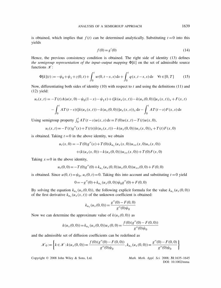
is obtained, which implies that f (t) can be determined analytically. Substituting t=0 into thisyields

f (0)=g′(0) (14)

Hence, the previous consistency condition is obtained. The right side of identity (13) definesthe semigroup representation of the input–output mapping �[k] on the set of admissible sourcefunctions K:

�[k](t) :=−�0+�1+z(0, t)+∫ t

0w(0, t−s,s)ds+

∫ t

0q(x, t−s,s)ds ∀t ∈[0,T ] (15)

Now, differentiating both sides of identity (10) with respect to t and using the definitions (11) and(12) yield:

ut (x, t) = −T (t)A(u(x,0)−�0(1−x)−�1x)+([k(ux (x, t))−k(ux (0,0))]ux (x, t))x +F(x, t)

−∫ t

0AT (t−s)([k(ux (x, t))−k(ux (0,0))]ux (x,s))x ds−

∫ t

0AT (t−s)F(x,s)ds

Using semigroup property∫ t0 AT (t−s)u(x,s)ds=T (0)u(x, t)−T (t)u(x,0),

ut (x, t)=−T (t)g′′(x)+T (t)((k(ux (x, t))−k(ux (0,0)))ux (x,0))x +T (t)F(x,0)

is obtained. Taking t=0 in the above identity, we obtain

ut (x,0) = −T (0)g′′(x)+T (0)(kux (ux (x,0))uxx (x,0)ux (x,0))

+(k(ux (x,0))−k(ux (0,0)))uxx (x,0))+T (0)F(x,0)

Taking x=0 in the above identity,

ut (0,0)=−T (0)g′′(0)+kux (ux (0,0))ux (0,0))uxx (0,0)+F(0,0)

is obtained. Since u(0, t)=�0, ut (0, t)=0. Taking this into account and substituting t=0 yield

0=−g′′(0)+kux (ux (0,0))�0g′′(0)+F(0,0)

By solving the equation kux (ux (0,0)), the following explicit formula for the value kux (ux (0,0))of the first derivative kux (ux (x, t)) of the unknown coefficient is obtained:

kux (ux (0,0))=g′′(0)−F(0,0)

g′′(0)�0

Now we can determine the approximate value of k(ux (0,0)) as

k(ux (0,0))=kux (ux (0,0))ux (0,0)=f (0)(g′′(0)−F(0,0))

g′′(0)�0

and the admissible set of diffusion coefficients can be redefined as

K0 :={k∈K :k(ux (0,0))= f (0)(g′′(0)−F(0,0))

g′′(0)�0,kux (ux (0,0))=

g′′(0)−F(0,0)

g′′(0)�0

}



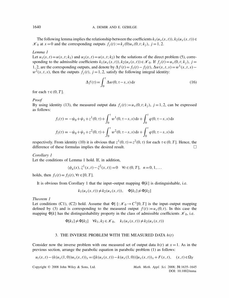
The following lemma implies the relationship between the coefficients k1(ux (x, t)),k2(ux (x, t))∈K0 at x=0 and the corresponding outputs f j (t) :=k j (0)ux (0, t;k j ), j =1,2.

Lemma 1Let u1(x, t)=u(x, t;k1) and u2(x, t)=u(x, t;k2) be the solutions of the direct problem (5), corre-sponding to the admissible coefficients k1(ux (x, t)),k2(ux (x, t))∈K0. If f j (t)=ux (0, t;k j ), j =1,2, are the corresponding outputs, and denote by � f (t)= f1(t)− f2(t), �w(x, t,s)=w1(x, t,s)−w2(x, t,s), then the outputs f j (t), j =1,2, satisfy the following integral identity:

� f (�)=∫ �

0�w(0,�−s,s)ds (16)

for each �∈(0,T ].ProofBy using identity (13), the measured output data f j (t) :=ux (0, t;k j ), j =1,2, can be expressedas follows:

f1(�) = −�0+�1+z1(0,�)+∫ �

0w1(0,�−s,s)ds+

∫ �

0q(0,�−s,s)ds

f2(�) = −�0+�1+z2(0,�)+∫ �

0w2(0,�−s,s)ds+

∫ �

0q(0,�−s,s)ds

respectively. From identity (10) it is obvious that z1(0,�)= z2(0,�) for each �∈(0,T ]. Hence, thedifference of these formulas implies the desired result. �

Corollary 1Let the conditions of Lemma 1 hold. If, in addition,

〈�n(x),�1(x, t)−�2(x, t)〉=0 ∀t ∈(0,T ], n=0,1, . . .

holds, then f1(t)= f2(t),∀t ∈[0,T ].It is obvious from Corollary 1 that the input–output mapping �[k] is distinguishable, i.e.

k1(ux (x, t)) �=k2(ux (x, t)), �[k1] �=�[k2]Theorem 1Let conditions (C1), (C2) hold. Assume that �[·] :K0→C1[0,T ] is the input–output mappingdefined by (3) and is corresponding to the measured output f (t) :=ux (0, t). In this case themapping �[k] has the distinguishability property in the class of admissible coefficients K0, i.e.

�[k1] �=�[k2] ∀k1,k2∈K0, k1(ux (x, t)) �=k2(ux (x, t))

3. THE INVERSE PROBLEM WITH THE MEASURED DATA h(t)

Consider now the inverse problem with one measured set of output data h(t) at x=1. As in theprevious section, arrange the parabolic equation in parabolic problem (1) as follows:

ut (x, t)−(k(ux (1,0))ux (x, t))x =([k(ux (x, t))−k(ux (1,0))]ux (x, t))x +F(x, t), (x, t)∈�T



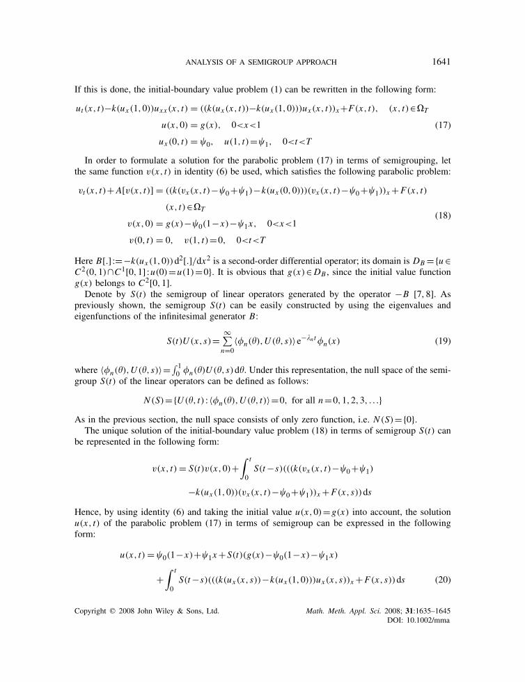
If this is done, the initial-boundary value problem (1) can be rewritten in the following form:

ut (x, t)−k(ux (1,0))uxx (x, t) = ((k(ux (x, t))−k(ux (1,0)))ux (x, t))x+F(x, t), (x, t)∈�T

u(x,0) = g(x), 0<x<1

ux (0, t) = �0, u(1, t)=�1, 0<t<T

(17)

In order to formulate a solution for the parabolic problem (17) in terms of semigrouping, letthe same function v(x, t) in identity (6) be used, which satisfies the following parabolic problem:

vt (x, t)+A[v(x, t)] = ((k(vx (x, t)−�0+�1)−k(ux (0,0)))(vx (x, t)−�0+�1))x +F(x, t)

(x, t)∈�T

v(x,0) = g(x)−�0(1−x)−�1x, 0<x<1

v(0, t) = 0, v(1, t)=0, 0<t<T

(18)

Here B[.] :=−k(ux (1,0))d2[.]/dx2 is a second-order differential operator; its domain is DB ={u∈C2(0,1)∩C1[0,1] :u(0)=u(1)=0}. It is obvious that g(x)∈DB , since the initial value functiong(x) belongs to C2[0,1].

Denote by S(t) the semigroup of linear operators generated by the operator −B [7, 8]. Aspreviously shown, the semigroup S(t) can be easily constructed by using the eigenvalues andeigenfunctions of the infinitesimal generator B:

S(t)U (x,s)=∞∑n=0

〈�n(�),U (�,s)〉e−�nt�n(x) (19)

where 〈�n(�),U (�,s)〉=∫ 10 �n(�)U (�,s)d�. Under this representation, the null space of the semi-

group S(t) of the linear operators can be defined as follows:

N (S)={U (�, t) : 〈�n(�),U (�, t)〉=0, for all n=0,1,2,3, . . .}As in the previous section, the null space consists of only zero function, i.e. N (S)={0}.

The unique solution of the initial-boundary value problem (18) in terms of semigroup S(t) canbe represented in the following form:

v(x, t) = S(t)v(x,0)+∫ t

0S(t−s)(((k(vx (x, t)−�0+�1)

−k(ux (1,0))(vx (x, t)−�0+�1))x +F(x,s))ds

Hence, by using identity (6) and taking the initial value u(x,0)=g(x) into account, the solutionu(x, t) of the parabolic problem (17) in terms of semigroup can be expressed in the followingform:

u(x, t) = �0(1−x)+�1x+S(t)(g(x)−�0(1−x)−�1x)

+∫ t

0S(t−s)(((k(ux (x,s))−k(ux (1,0)))ux (x,s))x +F(x,s))ds (20)



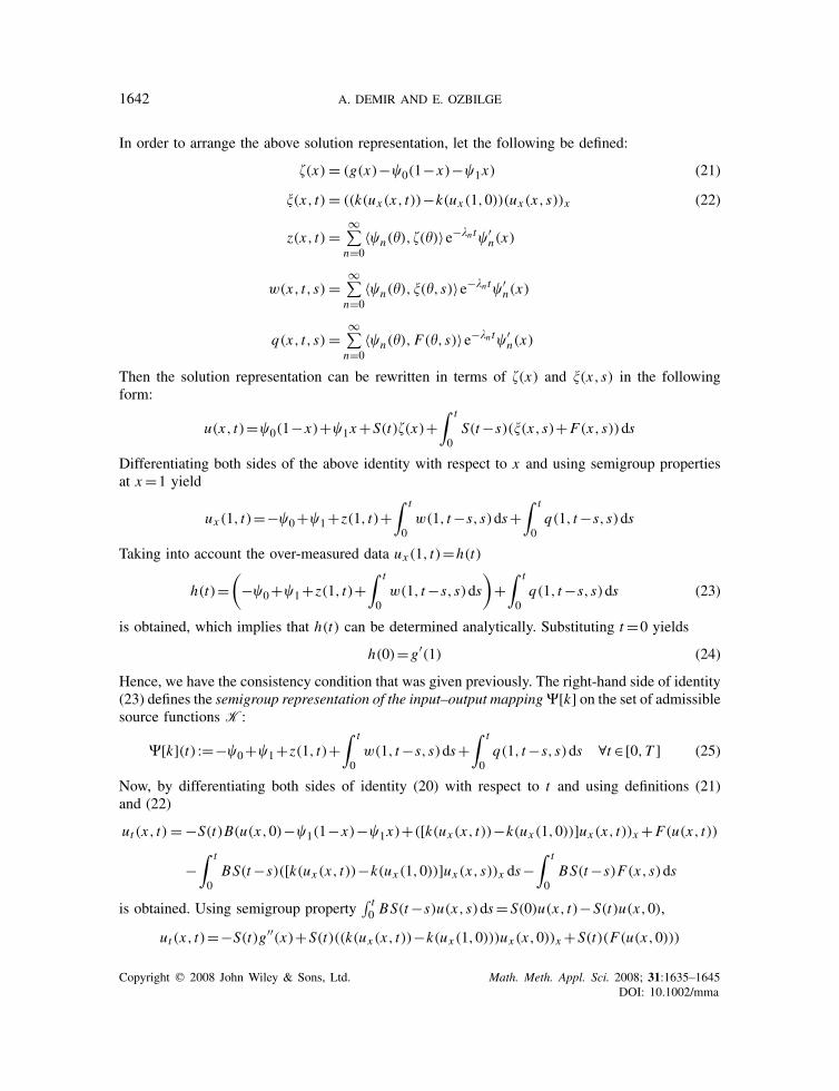
In order to arrange the above solution representation, let the following be defined:

�(x) = (g(x)−�0(1−x)−�1x) (21)

�(x, t) = ((k(ux (x, t))−k(ux (1,0))(ux (x,s))x (22)

z(x, t) =∞∑n=0

〈�n(�),�(�)〉e−�nt�′n(x)

w(x, t,s) =∞∑n=0

〈�n(�),�(�,s)〉e−�nt�′n(x)

q(x, t,s) =∞∑n=0

〈�n(�),F(�,s)〉e−�nt�′n(x)

Then the solution representation can be rewritten in terms of �(x) and �(x,s) in the followingform:

u(x, t)=�0(1−x)+�1x+S(t)�(x)+∫ t

0S(t−s)(�(x,s)+F(x,s))ds

Differentiating both sides of the above identity with respect to x and using semigroup propertiesat x=1 yield

ux (1, t)=−�0+�1+z(1, t)+∫ t

0w(1, t−s,s)ds+

∫ t

0q(1, t−s,s)ds

Taking into account the over-measured data ux (1, t)=h(t)

h(t)=(

−�0+�1+z(1, t)+∫ t

0w(1, t−s,s)ds

)+

∫ t

0q(1, t−s,s)ds (23)

is obtained, which implies that h(t) can be determined analytically. Substituting t=0 yields

h(0)=g′(1) (24)

Hence, we have the consistency condition that was given previously. The right-hand side of identity(23) defines the semigroup representation of the input–output mapping�[k] on the set of admissiblesource functions K:

�[k](t) :=−�0+�1+z(1, t)+∫ t

0w(1, t−s,s)ds+

∫ t

0q(1, t−s,s)ds ∀t ∈[0,T ] (25)

Now, by differentiating both sides of identity (20) with respect to t and using definitions (21)and (22)

ut (x, t) = −S(t)B(u(x,0)−�1(1−x)−�1x)+([k(ux (x, t))−k(ux (1,0))]ux (x, t))x +F(u(x, t))

−∫ t

0BS(t−s)([k(ux (x, t))−k(ux (1,0))]ux (x,s))x ds−

∫ t

0BS(t−s)F(x,s)ds

is obtained. Using semigroup property∫ t0 BS(t−s)u(x,s)ds= S(0)u(x, t)−S(t)u(x,0),

ut (x, t)=−S(t)g′′(x)+S(t)((k(ux (x, t))−k(ux (1,0)))ux (x,0))x +S(t)(F(u(x,0)))



is obtained. Taking t=0 in the above identity,

ut (x,0) = −S(0)g′′(x)+S(0)(kux (ux (x,0))uxx (x,0)ux (x,0))

+(k(ux (x,0))−k(ux (1,0)))uxx (x,0))+S(0)F(x,0)

is obtained. Taking x=1 in the above identity,

ut (1,0)=−S(0)g′′(1)+kux (ux (1,0))ux (1,0))uxx (1,0)+F(1,0)

is obtained. Since u(1, t)=�1, ut (1, t)=0. Taking this into account and substituting t=0 yield

0=−g′′(1)+kux (ux (1,0))�1g′′(1)+F(1,0)

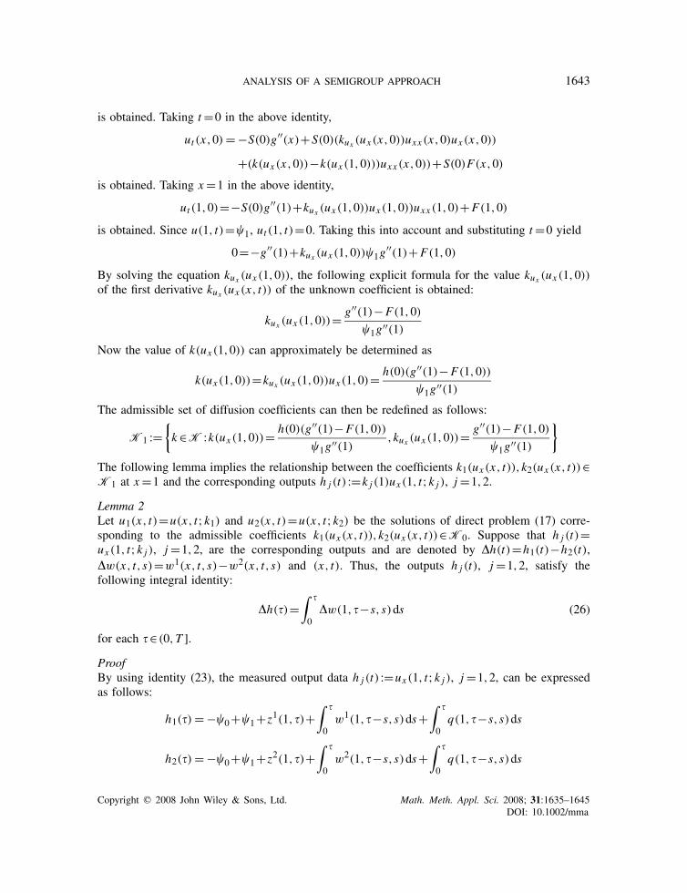
By solving the equation kux (ux (1,0)), the following explicit formula for the value kux (ux (1,0))of the first derivative kux (ux (x, t)) of the unknown coefficient is obtained:

kux (ux (1,0))=g′′(1)−F(1,0)

�1g′′(1)Now the value of k(ux (1,0)) can approximately be determined as

k(ux (1,0))=kux (ux (1,0))ux (1,0)=h(0)(g′′(1)−F(1,0))

�1g′′(1)The admissible set of diffusion coefficients can then be redefined as follows:

K1 :={k∈K :k(ux (1,0))= h(0)(g′′(1)−F(1,0))

�1g′′(1),kux (ux (1,0))=

g′′(1)−F(1,0)

�1g′′(1)

}

The following lemma implies the relationship between the coefficients k1(ux (x, t)),k2(ux (x, t))∈K1 at x=1 and the corresponding outputs h j (t) :=k j (1)ux (1, t;k j ), j =1,2.

Lemma 2Let u1(x, t)=u(x, t;k1) and u2(x, t)=u(x, t;k2) be the solutions of direct problem (17) corre-sponding to the admissible coefficients k1(ux (x, t)),k2(ux (x, t))∈K0. Suppose that h j (t)=ux (1, t;k j ), j =1,2, are the corresponding outputs and are denoted by �h(t)=h1(t)−h2(t),�w(x, t,s)=w1(x, t,s)−w2(x, t,s) and (x, t). Thus, the outputs h j (t), j =1,2, satisfy thefollowing integral identity:

�h(�)=∫ �

0�w(1,�−s,s)ds (26)

for each �∈(0,T ].ProofBy using identity (23), the measured output data h j (t) :=ux (1, t;k j ), j =1,2, can be expressedas follows:

h1(�) = −�0+�1+z1(1,�)+∫ �

0w1(1,�−s,s)ds+

∫ �

0q(1,�−s,s)ds

h2(�) = −�0+�1+z2(1,�)+∫ �

0w2(1,�−s,s)ds+

∫ �

0q(1,�−s,s)ds



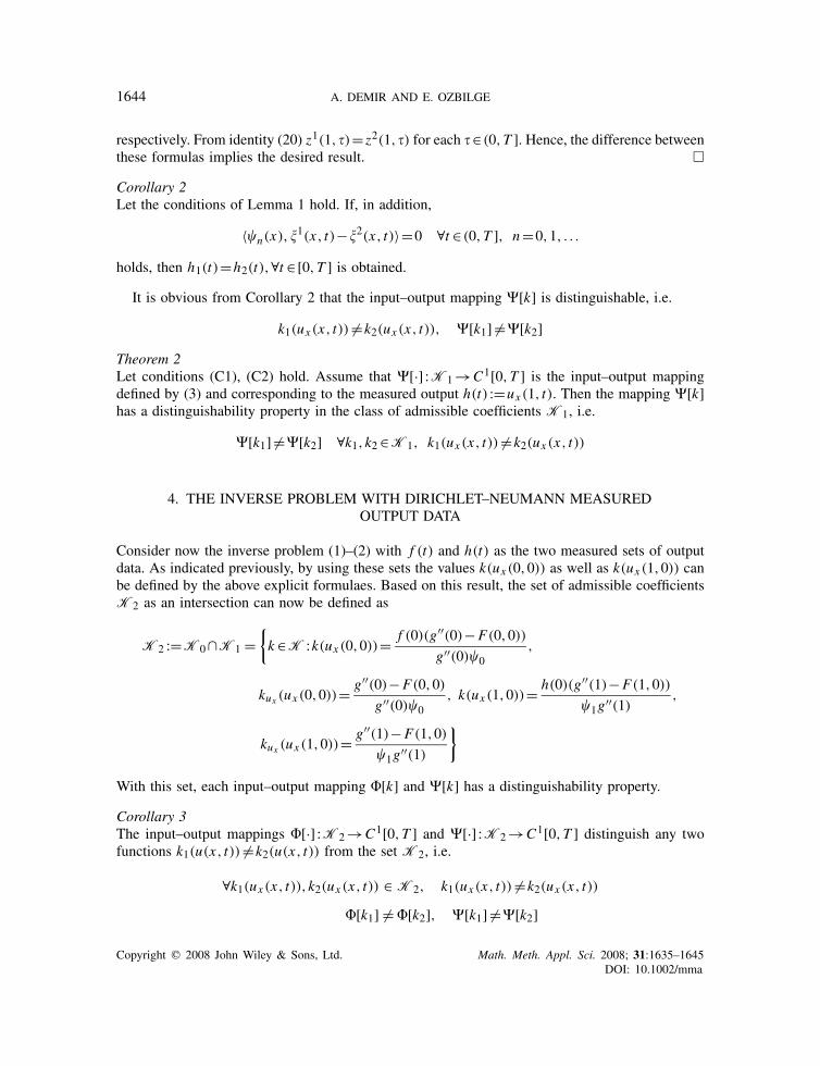
respectively. From identity (20) z1(1,�)= z2(1,�) for each �∈(0,T ]. Hence, the difference betweenthese formulas implies the desired result. �

Corollary 2Let the conditions of Lemma 1 hold. If, in addition,

〈�n(x),�1(x, t)−�2(x, t)〉=0 ∀t ∈(0,T ], n=0,1, . . .

holds, then h1(t)=h2(t),∀t ∈[0,T ] is obtained.It is obvious from Corollary 2 that the input–output mapping �[k] is distinguishable, i.e.

k1(ux (x, t)) �=k2(ux (x, t)), �[k1] �=�[k2]Theorem 2Let conditions (C1), (C2) hold. Assume that �[·] :K1→C1[0,T ] is the input–output mappingdefined by (3) and corresponding to the measured output h(t) :=ux (1, t). Then the mapping �[k]has a distinguishability property in the class of admissible coefficients K1, i.e.

�[k1] �=�[k2] ∀k1,k2∈K1, k1(ux (x, t)) �=k2(ux (x, t))

4. THE INVERSE PROBLEM WITH DIRICHLET–NEUMANN MEASUREDOUTPUT DATA

Consider now the inverse problem (1)–(2) with f (t) and h(t) as the two measured sets of outputdata. As indicated previously, by using these sets the values k(ux (0,0)) as well as k(ux (1,0)) canbe defined by the above explicit formulaes. Based on this result, the set of admissible coefficientsK2 as an intersection can now be defined as

K2 :=K0∩K1 ={k∈K :k(ux (0,0))= f (0)(g′′(0)−F(0,0))

g′′(0)�0,

kux (ux (0,0))=g′′(0)−F(0,0)

g′′(0)�0, k(ux (1,0))= h(0)(g′′(1)−F(1,0))

�1g′′(1),

kux (ux (1,0))=g′′(1)−F(1,0)

�1g′′(1)

}

With this set, each input–output mapping �[k] and �[k] has a distinguishability property.

Corollary 3The input–output mappings �[·] :K2→C1[0,T ] and �[·] :K2→C1[0,T ] distinguish any twofunctions k1(u(x, t)) �=k2(u(x, t)) from the set K2, i.e.

∀k1(ux (x, t)),k2(ux (x, t)) ∈ K2, k1(ux (x, t)) �=k2(ux (x, t))

�[k1] �= �[k2], �[k1] �=�[k2]



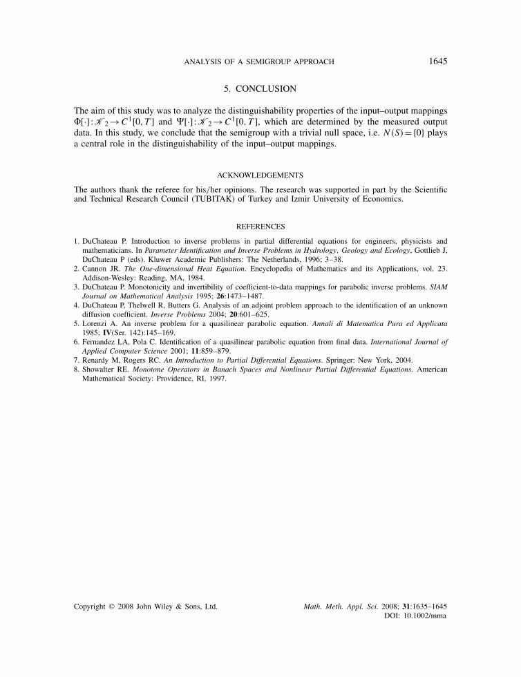
5. CONCLUSION

The aim of this study was to analyze the distinguishability properties of the input–output mappings�[·] :K2→C1[0,T ] and �[·] :K2→C1[0,T ], which are determined by the measured outputdata. In this study, we conclude that the semigroup with a trivial null space, i.e. N (S)={0} playsa central role in the distinguishability of the input–output mappings.

ACKNOWLEDGEMENTS

The authors thank the referee for his/her opinions. The research was supported in part by the Scientificand Technical Research Council (TUBITAK) of Turkey and Izmir University of Economics.

REFERENCES

1. DuChateau P. Introduction to inverse problems in partial differential equations for engineers, physicists andmathematicians. In Parameter Identification and Inverse Problems in Hydrology, Geology and Ecology, Gottlieb J,DuChateau P (eds). Kluwer Academic Publishers: The Netherlands, 1996; 3–38.

2. Cannon JR. The One-dimensional Heat Equation. Encyclopedia of Mathematics and its Applications, vol. 23.Addison-Wesley: Reading, MA, 1984.

3. DuChateau P. Monotonicity and invertibility of coefficient-to-data mappings for parabolic inverse problems. SIAMJournal on Mathematical Analysis 1995; 26:1473–1487.

4. DuChateau P, Thelwell R, Butters G. Analysis of an adjoint problem approach to the identification of an unknowndiffusion coefficient. Inverse Problems 2004; 20:601–625.

5. Lorenzi A. An inverse problem for a quasilinear parabolic equation. Annali di Matematica Pura ed Applicata1985; IV(Ser. 142):145–169.

6. Fernandez LA, Pola C. Identification of a quasilinear parabolic equation from final data. International Journal ofApplied Computer Science 2001; 11:859–879.

7. Renardy M, Rogers RC. An Introduction to Partial Differential Equations. Springer: New York, 2004.8. Showalter RE. Monotone Operators in Banach Spaces and Nonlinear Partial Differential Equations. American

Mathematical Society: Providence, RI, 1997.


Documents

Analysis of a semigroup approach in the inverse problem of identifying an unknown coefficient