Analysis of a Painted Body Storage System An investigation of buffer capacity and solutions to storage system expansion

Master of Science Thesis in the Programme Systems, Control and Mechatronics

JONAS AINOUZ

Chalmers University of Technology

Department of Product and Production Development

Göteborg, Sweden, July 2011

ii

Analysis of a Painted Body Storage System An investigation of buffer capacity and solutions to storage system expansion

JONAS C.Y AINOUZ

© JONAS C.Y AINOUZ, July 2011

Master thesis work 2011

Chalmers University of Technology

Department of Product and Production Development

SE-412 96 Göteborg

Sweden

Telephone + 46 (0)31-772 1000

Performed at: Scania CV AB

Sandåsavägen 7, 572 29 Oskarshamn

Supervisors: Sten Gunnarsson

Scania CV AB

Sandåsavägen 7, 572 29 Oskarshamn

Per Nyquist

Department of Product and Production Development

Chalmers University of Technology, 412 96 Göteborg

Examiner: Björn Johansson

Department of Product and Production Development

Chalmers University of Technology, 412 96 Göteborg

iii

Preface This report is the result of a 30 points Master of Science thesis at Chalmers University of

technology performed during the spring 2011. The work was conducted at Scania CV AB in

Oskarshamn with the goal of investigating the demands in buffer capacity as well as alternative

solutions for the expansion of the painted body storage system.

This thesis work marks the end of my studies at the masters programme Systems, Control and

Mechatronics at Chalmers University of technology. I would like to thank all the people who have

contributed to this work and supported me during this period. I would especially like to thank my

supervisor at Scania, Sten Gunnarsson, for all his support and many ideas. I would also like to

thank John Larsson, Pernilla Zackrisson and all the other employees at Scania who always

answered all of my many questions. Finally, I would like to thank my supervisor at Chalmers, Per

Nyquist, and my examinator Björn Johansson.

Göteborg, Sweden, July 2011

iv

Abstract In most automotive factories, storage systems are positioned in between processes in order to

enable batching and handle disturbances in the process. Typically, these storages are either

conveyor based selectivity banks (SB) or automated storage and retrieval systems (AS/RS).

At the Scania plant in Oskarshamn, where truck cabs are manufactured, a number of storages of

AS/RS type are located in between different parts of the plant. One of these is the painted body

storage, situated between the paint shop and the trim shop (general assembly). The objective of

this storage system is to handle disturbances and the different working hours in the paint shop

and trim shop, but also to enable correction of the production sequence. This storage system has

been identified as a future bottleneck, and as the company is preparing to increase the

production capacity, appropriate measures have to be taken in order to increase the capacity of

this storage system.

In this thesis, different solutions on how to increase the throughput and buffer space of the PBS

are investigated. The main proposed solution is to expand the AS/RS with a parallel selectivity

bank. This thesis describes an example of such a configuration where a number of parallel

conveyor lanes are used to increase the throughput as well as the storage capacity of the system.

Presented in this thesis is also a developed algorithm for choosing where to store arriving cabs in

order to optimize the flow. Simulations results showed that the presented solution could handle

large increases of the production rate. However, an analysis of the necessary buffer capacity

showed that the available buffer space would have to be increased proportionally to the increase

in production rate, thus making a selectivity bank a costly solution.

Keywords: Automotive manufacturing; Storage systems;, AS/RS; selectivity bank; Simulation.

v

Table of content

1. Introduction ..................................................................................................................................... 1

1.1 Background .............................................................................................................................. 1

1.2 Objective and scope ................................................................................................................ 2

1.3 Methodology ........................................................................................................................... 2

1.4 Scania AB ................................................................................................................................. 3

2. Theory .......................................................................................................................................... 4

2.1 Sequencing in mixed model assembly .................................................................................... 4

2.2 Storage systems ....................................................................................................................... 4

3. Description of the production process ............................................................................................ 5

3.1 The press shop ......................................................................................................................... 5

3.2 The body shop ......................................................................................................................... 5

3.3 The Paint shop ......................................................................................................................... 6

3.4 The trim shop .......................................................................................................................... 6

3.5 Buffers ..................................................................................................................................... 6

4. Process Analysis ............................................................................................................................... 7

4.1 Car sequencing at Scania ......................................................................................................... 7

4.2 The painted body storage AS/RS ............................................................................................. 7

4.3 Modeling of the AS/RS ............................................................................................................ 8

Storage policy .................................................................................................................................. 9

Order policy ..................................................................................................................................... 9

Sequencing ...................................................................................................................................... 9

4.4 Arrivals ..................................................................................................................................... 9

4.5 Sequence deviations .............................................................................................................. 10

4.6 Trim shop data ....................................................................................................................... 10

4.7 Production Schedule ............................................................................................................. 11

5. Throughput analysis ...................................................................................................................... 12

5.1 Performance analysis of the AS/RS ....................................................................................... 12

Simulation of PBS throughput ....................................................................................................... 13

Simulation of fully manned night shift .......................................................................................... 13

5.2 Optimization of the AS/RS ..................................................................................................... 14

Simulation of moved input ............................................................................................................ 15

vi

5.3 Parallel selectivity bank ......................................................................................................... 16

Modeling of AS/RS – PSB configuration ........................................................................................ 16

Retrieval policy .............................................................................................................................. 17

Store policy .................................................................................................................................... 17

Choice of conveyor lane ................................................................................................................ 18

Choice of storage system .............................................................................................................. 18

Simulation of AS/RS – PSB configuration ...................................................................................... 18

6. Buffer capacity ............................................................................................................................... 21

6.1 Difficulties with simulation .................................................................................................... 21

6.2 Buffer levels ........................................................................................................................... 22

6.3 Statistical analysis .................................................................................................................. 22

Observed buffer levels .................................................................................................................. 22

Disturbance probability ................................................................................................................. 23

Estimation of necessary buffer space ........................................................................................... 23

6.4 Total necessary buffer capacity ............................................................................................. 24

7. Conclusions .................................................................................................................................... 26

8. Discussion ...................................................................................................................................... 27

References ............................................................................................................................................. 28

Appendices ............................................................................................................................................... i

Appendix A – AS/RS data and calculations ........................................................................................... i

Appendix B – Working schedules ........................................................................................................ iii

Appendix C – Data representation ...................................................................................................... iii

Arrival times .................................................................................................................................... iii

Down time and MTTF in the trim shop ........................................................................................... iv

Appendix D - Algorithms....................................................................................................................... v

Algorithm 1 - Sequencing Algorithm ................................................................................................ v

Example 2 of a sequencing operation – AS/RS with parallel selectivity bank ................................. ix

Algorithm 2 - Algorithm for choosing conveyor lane ....................................................................... x

Control Method ................................................................................................................................... xi

Appendix E – Buffer capacity ............................................................................................................. xiii

Data representation ...................................................................................................................... xiii

Calculations of probability of buffer variations ............................................................................. xiii

Probability of buffer variations ...................................................................................................... xv

vii

viii

Abbreviations AS/RS Automated storage and retrieval system

S/RM Storage and retrieval machine

PBS Painted body storage

SB Selectivity bank

PSB Parallel selectivity bank

1

1. Introduction

1.1 Background Automotive factories generally consist of five main shops: The press shop, body shop, paint shop,

powertrain shop, and trim shop (general assembly). As a result of the very nature of the tasks

performed in each shop, they all apply different manufacturing principles. While the body shop

prefers to produce batches of products of the same models, the paint shop produces batches of

same-colored products. The assembly shop on the other hand, operating by the principles of mixed-

model production, focuses on smoothing out the production with a mix of products of different

models and with different options. On top of this is a planned sequence which has to be respected in

order for the product to be delivered to the customer on time.

In order to handle the different production policies of the shops, intermediate storage systems are

placed between shops. These storages enable the production sequence of each shop to be

optimized, but they also act as buffers, reducing the effects of disturbances in the process (Ribeiro,

Barata, & Sousa, 2009). Three storage systems are considered especially important and are installed

in most automotive factories. These are positioned between the body shop and the paint shop,

inside the paint shop between the primary coating process and the top coating process, and between

the paint shop and the trim shop.

The background of this thesis is ongoing preparations at Scania AB for an increase of the production

of trucks. At the plant in Oskarshamn, Scania produces truck cabs, which are then shipped to

different locations in Europe for further assembly. The objective of preparing the plant to handle the

predefined future production volumes presents a major challenge in identifying all the possible

bottlenecks in the process and making necessary improvements. One component in the process

which has been identified as a bottleneck is the painted body storage (PBS), located between the

paint shop and trim shop. The PBS consists of a one-aisle automated storage and retrieval system

(AS/RS) with one storage/retrieval machine (S/RM). The major concern with this storage is the

limited throughput, but there is also a question of the size of the storage in order to cope with the

different production volumes.

The targeted production volumes are defined as a number of steps presented in Table 1. The

numbers specify the average production volumes of the paint shop.

Table 1. Predefined production volumes.

The main solution which so far has been considered to the problem of limited capacity of the PBS is

to expand the current AS/RS or to build a new one. This is however a very expensive solution which

makes it important to investigate other possible solutions as well as to determine the actual

demands in terms of buffer capacity.

Predefined step Production Volume

Step 3 (Current production capacity) 285 cabs / day

Step 3.5 350 cabs / day

Step 4 410 cabs / day

Step 5 490 cabs / day

2

1.2 Objective and scope The purpose of this thesis is to investigate the capacity demands of the PBS for the predefined

production volumes, as well as to investigate alternative solutions on how to increase the capacity of

the buffer. To accomplish these objectives, this work aims to identify the critical factors which are

influenced by the performance of the PBS. Control methods also have to be developed in order to

demonstrate the feasibility of solutions by the means of simulation. Also, an analysis of the necessary

buffer size is to be performed for the future production volumes.

The company is currently working on plans on how to expand and upgrade the process to be able to

handle step 3.5. However, a solution which handles this step also has to be expandable to handle

larger production volumes. Presented solutions are supposed to act as an alternative to expanding

the current AS/RS or building a new one.

Initially it was included in the project scope to update an existing simulation model of the production

plant implemented in the simulation software Extend. The idea was to then use this to carry out

necessary simulations. However, during the project planning phase it was discovered that this

method would not be a very suitable way to reach the stated goals. Therefore, with the consent of

Scania representatives, it was decided that tools and methods determined most suitable in order to

reach the goals should be used instead.

This work is limited to the PBS. Therefore, all processes in the plant affecting the PBS will be dealt

with in their current state. This means that no efforts will be made in trying to improve any other

parts of the plant that might affect or be affected by the PBS.

1.3 Methodology The project started out with an analysis of the system in the form of interviews with technicians and

planning personnel in order to gain understanding of the problem at hand. A literature study was

then performed with the intention of gaining deeper understanding of the subject and to investigate

different approaches to the problem. The project then continued with planning and choosing a

method of how to approach the problem. MATLAB was chosen as the main tool for simulation based

on the simplicity it provides in writing algorithms and manipulating data. Automod was also used to

some extent in order to validate the MATLAB model but also to investigate the effects that the PBS

has on adjacent processes.

The input data to the simulation models was for most part gathered in the form of raw data from the

company database and filtered to be used as input data. Some data were also measured manually or

taken from a parallel simulation project.

3

1.4 Scania AB Scania AB is a Swedish manufacturer of heavy trucks, buses and diesel engines. A major part of the

company operations is performed in Södertälje, Sweden, where the head office is located and where

all research and development takes place. However, production and sales are worldwide with

production facilities in Sweden, France, Netherlands Argentina, Brazil, Poland and Russia, and sales

and service in over 100 countries. At the Scania plant in Oskarshamn, fully assembled truck cabs are

produced for the manufacturing of trucks in Europe. The major owner of Scania is the German

automotive company Volkswagen AG, and the company has approximately 35,500 employees

worldwide (Scaniakoncernen, 2011).

4

2. Theory In this chapter, theory concerning mixed model assembly and different types of storage systems is

presented in order to make it easier for the reader to comprehend the work presented in this thesis.

2.1 Sequencing in mixed model assembly In the automotive industry in general, the customer demand of product variability has led companies

to offer a large number of different options, creating a huge variety of models of each product. And

since the demand of one specific model is often insufficient to justify the dedication of resources for

that particular model, the models have to share resources. This is also the case at the Scania plant,

where one large impact of this is in the trim shop, where all the different cab models are assembled

on the same lines. The problem with this becomes obvious when you add the fact that the lead times

at certain stations in the trim shop varies significantly between different product models and options.

The general approach to this problem is to try to avoid or minimize work overload by smoothing out

the flow of products to the trim shop. This can be done either by mixed-model sequencing, or car

sequencing (Boysen, Scholl, & Woppere).

In mixed-model sequencing, parameters such as operation times, worker movements and station

borders are taken into account to generate a detailed schedule for the flow of products. Car

sequencing is a more implicit method which aims to minimize work overload by formulating a set of

spacing constraints. These constraints are often defined as: At most H products with option O are

allowed among N subsequent positions. Work overload can then be minimized by finding a sequence

which minimizes the number of broken spacing constraints.

2.2 Storage systems Typically, storage systems in automotive production plants are either of the type selectivity bank

(SB), or automated storage and retrieval system (AS/RS). An AS/RS generally consists of a number of

parallel racks divided into a number of bins. In the aisles between the racks, storage and retrieval

machines (S/RM) operate in both vertical and horizontal direction. These machines can store or

retrieve objects from any of the bins in the racks on either side of the aisles in which the S/RM is

operating. Computer systems are used to keep track of the location of stored objects as well as to

determine the most suitable location to store an arriving object.

Selectivity banks on the other hand consist of a number of parallel transportation lanes. When an

object arrives to the bank, a computer algorithm is used to calculate the most suitable lane in which

to store the object. Since the flow of objects in each lane is first in first out (FIFO), it will not be

possible to extract the object until all the objects ahead in the same lane have all been extracted.

However, in some SB, feedback loops are used to return objects to the entrance to the bank in order

to avoid blocking. The major drawbacks with this storage system is that the footprint becomes very

large and most importantly, only objects in front position of each lane can be chosen for extraction

Compared to the SB, the AS/RS has the advantages of allowing more candidates to be taken into

account for retrieval, and minimizing the footprint of the storage buffer since objects can be stacked

vertically in racks. On the other hand, it is very expensive to build. It also has a drawback of limited

throughput which is dependent on the operating speed of the S/RM. (Moon, Song, & Ha, 2005). At

the Scania plant in Oskarshamn, all of the storage systems are of the type AS/RS.

5

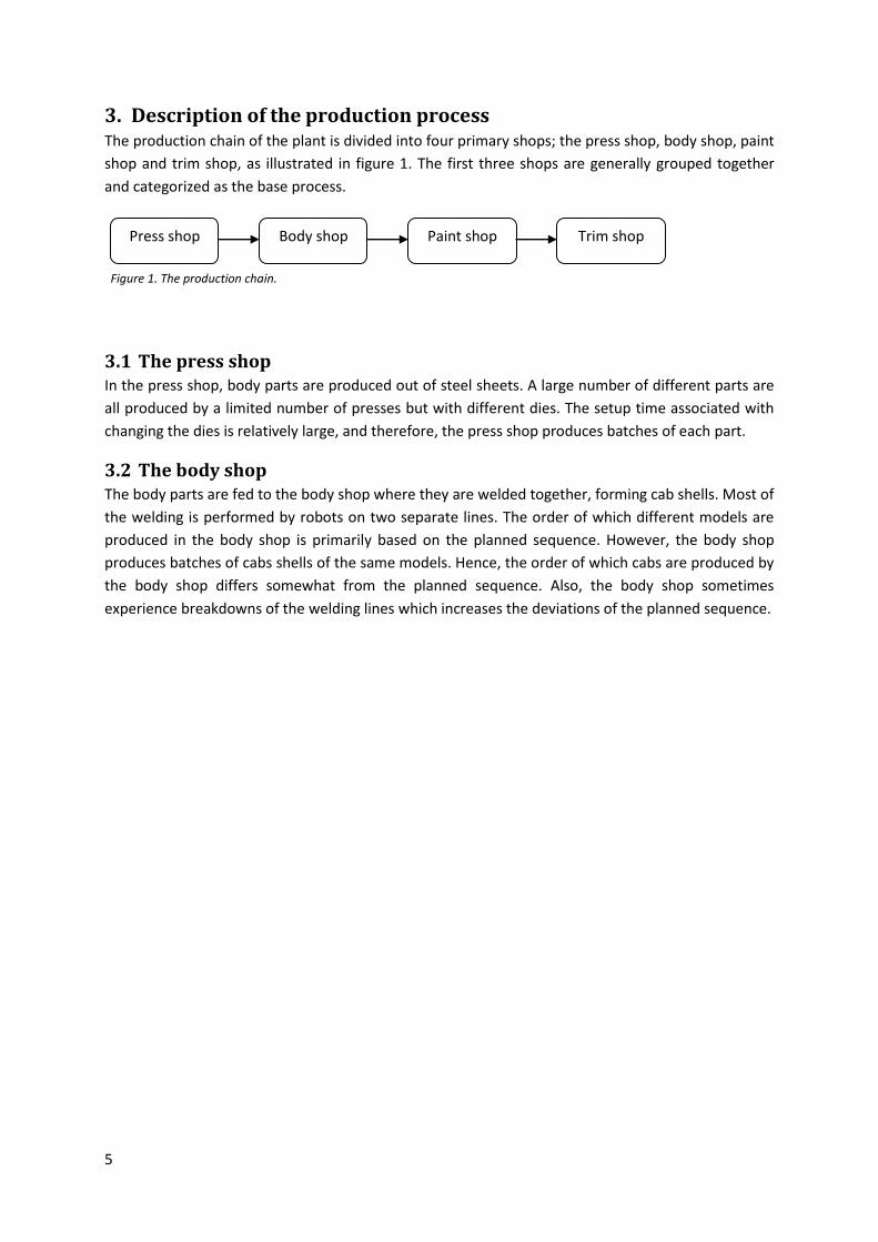
3. Description of the production process The production chain of the plant is divided into four primary shops; the press shop, body shop, paint

shop and trim shop, as illustrated in figure 1. The first three shops are generally grouped together

and categorized as the base process.

3.1 The press shop In the press shop, body parts are produced out of steel sheets. A large number of different parts are

all produced by a limited number of presses but with different dies. The setup time associated with

changing the dies is relatively large, and therefore, the press shop produces batches of each part.

3.2 The body shop The body parts are fed to the body shop where they are welded together, forming cab shells. Most of

the welding is performed by robots on two separate lines. The order of which different models are

produced in the body shop is primarily based on the planned sequence. However, the body shop

produces batches of cabs shells of the same models. Hence, the order of which cabs are produced by

the body shop differs somewhat from the planned sequence. Also, the body shop sometimes

experience breakdowns of the welding lines which increases the deviations of the planned sequence.

Press shop

Body shop

Paint shop

Trim shop

Figure 1. The production chain.

6

3.3 The Paint shop When the cab shells enter the paint shop, they are first subject to a primary coating process where

statically charged primer in powder form is sprayed on to the cabs. The cabs are then sent into an

oven where the powder melts, forming a layer of paint primer.

After the primary coating process, cabs are sent to the top coating process where they are grouped

in color batches. These batches are then spray painted on one of three lines, of which one is fully

automated with painting robots. In general, cabs with high frequent colors are grouped in large

batches and then painted on the automated line, while cabs with low frequent colors are grouped in

smaller batches or painted separately on one of the manual paint lines. The batching in the top

coating process is a consequence of the need to purge the painting equipment between each color

change, which results in a loss of both time and paint. The batching in the paint shop results in large

deviations from the planned sequence. This is especially the case when cabs are painted in metallic

colors. The capacity to paint metallic colors in the paint shop is limited to a fixed number per week,

resulting in the need to paint some cabs several days in advance. Also, the painting process is of

nature such that it is hard to achieve a perfect result each time. As a result, there is a frequent need

of manual touch up and sometimes repaint of entire cabs. Before cabs exits the paint shop they pass

the insulation line and the anti-corrosion line (ACL). The flow on these lines is first in, first out (FIFO),

meaning that the order in which cabs enter the line is the same as the order in which they exit. When

cabs exit the ACL line they are subject to an inspection. If the inspection is passed, the cabs are sent

to the PBS, otherwise they are extracted from the flow and sent for touch-up.

3.4 The trim shop When it is time for a cab to be assembled, it is retrieved from the PBS and sent to the trim shop. The

sequence in which cabs are assembled are primarily based on the planned sequence, but the

assembly also apply spacing rules for certain cab models and options. Since there is no possibility to

extract a cab from the assembly line, the flow here is always FIFO.

Finally, when a cab has been assembled and it has passed inspection, it is shipped to a different

location for final assembly of chassis and power train.

3.5 Buffers As mentioned earlier there are three main buffers in the process, all of AS/RS type. The objective of

the first buffer, situated between the body shop and the primary coating process, is to handle

disturbances in the two shops, and to restore the planned sequence after the body shop. The second

buffer, situated between the primary coating process and the top coating process, is primarily used

for batching of same colored cabs, but also to handle disturbances.

The third buffer, referred to as the painted body storage (PBS), which is the focus of this work, is

situated between the paint shop and the trim shop. The objectives of this buffer is to restore the

planned sequence, handle disturbances and enable sequencing of cabs to the trim shop, but also to

handle the different working times in the base process and the trim shop.

All of these buffers are commonly found in any automotive manufacturing plant. However, it is the

PBS that has gained the most attention in literature. A common topic is the resequencing of cars with

a PBS of selectivity bank type (Boysen, Scholl, & Woppere).

7

4. Process Analysis In this chapter, a detailed description of the AS/RS is described. Other factors needed to model the

process is also presented as well as data used in simulations.

4.1 Car sequencing at Scania The car sequencing method is applied in the trim shop at the Scania plant. The spacing constraints

are defined as maximum allowed frequency (f) for certain options and models (O), where a maximum

frequency of 3 means that at most every third successive cab is allowed to have option O. Each

spacing constraint is assigned a priority, ranging from 1 to the number of rules, where the spacing

constraint with priority 1 is the most important not to violate, and so on. A list with the spacing

constraints used by the trim shop today and the percentage of cabs having the corresponding

options is shown in table 2.

Priority Model/Option (O) Max Frequency (f) Cabs with option O

1 P-Cab 3 23.5 %

2 Right-hand drive 3 15.6 %

3 Contrast-tape 2 26.4 %

4 Topline 2 12.5 %

5 Painted plastic details 5 33.7 %

6 Dual tool hatches 3 7.5 % Table 2. Spacing constraints used in the trim shop and percentage of cabs with corresponding option.

While it is possible for one cab to have several options, some of the options cannot be combined. For

example, a cab cannot be both a P-cab and a Topline since these options refer to two completely

different cab models.

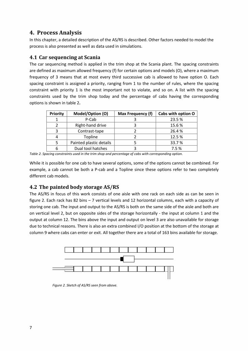
4.2 The painted body storage AS/RS The AS/RS in focus of this work consists of one aisle with one rack on each side as can be seen in

figure 2. Each rack has 82 bins – 7 vertical levels and 12 horizontal columns, each with a capacity of

storing one cab. The input and output to the AS/RS is both on the same side of the aisle and both are

on vertical level 2, but on opposite sides of the storage horizontally - the input at column 1 and the

output at column 12. The bins above the input and output on level 3 are also unavailable for storage

due to technical reasons. There is also an extra combined I/O position at the bottom of the storage at

column 9 where cabs can enter or exit. All together there are a total of 163 bins available for storage.

Figure 2. Sketch of AS/RS seen from above.

8

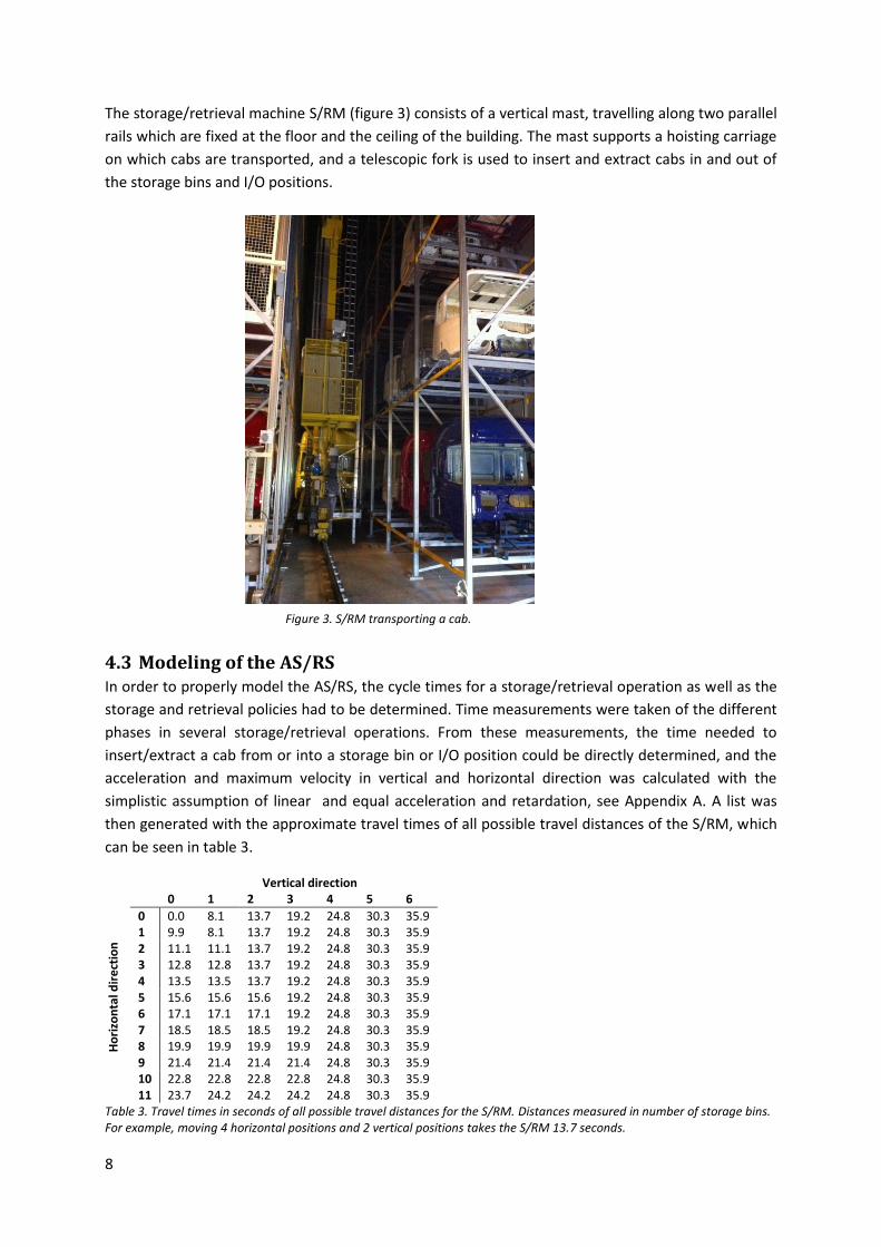
The storage/retrieval machine S/RM (figure 3) consists of a vertical mast, travelling along two parallel

rails which are fixed at the floor and the ceiling of the building. The mast supports a hoisting carriage

on which cabs are transported, and a telescopic fork is used to insert and extract cabs in and out of

the storage bins and I/O positions.

4.3 Modeling of the AS/RS In order to properly model the AS/RS, the cycle times for a storage/retrieval operation as well as the

storage and retrieval policies had to be determined. Time measurements were taken of the different

phases in several storage/retrieval operations. From these measurements, the time needed to

insert/extract a cab from or into a storage bin or I/O position could be directly determined, and the

acceleration and maximum velocity in vertical and horizontal direction was calculated with the

simplistic assumption of linear and equal acceleration and retardation, see Appendix A. A list was

then generated with the approximate travel times of all possible travel distances of the S/RM, which

can be seen in table 3.

Vertical direction

Ho

rizo

nta

l dir

ect

ion

0 1 2 3 4 5 6

0 0.0 8.1 13.7 19.2 24.8 30.3 35.9 1 9.9 8.1 13.7 19.2 24.8 30.3 35.9 2 11.1 11.1 13.7 19.2 24.8 30.3 35.9 3 12.8 12.8 13.7 19.2 24.8 30.3 35.9 4 13.5 13.5 13.7 19.2 24.8 30.3 35.9 5 15.6 15.6 15.6 19.2 24.8 30.3 35.9 6 17.1 17.1 17.1 19.2 24.8 30.3 35.9 7 18.5 18.5 18.5 19.2 24.8 30.3 35.9 8 19.9 19.9 19.9 19.9 24.8 30.3 35.9 9 21.4 21.4 21.4 21.4 24.8 30.3 35.9 10 22.8 22.8 22.8 22.8 24.8 30.3 35.9 11 23.7 24.2 24.2 24.2 24.8 30.3 35.9

Table 3. Travel times in seconds of all possible travel distances for the S/RM. Distances measured in number of storage bins. For example, moving 4 horizontal positions and 2 vertical positions takes the S/RM 13.7 seconds.

Figure 3. S/RM transporting a cab.

9

Storage policy

The AS/RS always stores cabs in the lowest vertical level possible and as close to the output position

as possible. The reason for this is that vertical travel of the S/RM is much slower than that of

horizontal travelling, as can be seen in table 3. If the S/RM is to move 4 or more vertical position, the

travelling time will always be decided by the time for vertical travel regardless of the horizontal

distance the S/RM has to travel.

Order policy

The order policy of the AS/RS is of first-come, first-served type. Whenever an order arrives to the

AS/RS it is placed in a queue, and when the AS/RS becomes idle it checks if there are any orders in

this queue. If there are orders in this queue, it serves the order that first arrived to the queue.

Sequencing

When retrieving cabs from the AS/RS, two set of parameters are taken into account: Planned

sequence and spacing constraints. The retrieval procedure used today is as follows:

1. All cabs available in the AS/RS are sorted based on the planned sequence.

2. A number (usually 16) of the cabs with the least time until due date are then chosen for retrieval.

3. The list of cabs chosen for retrieval is then re-arranged in order to minimize the number of

violated spacing constraints. This is done by going through the list one cab at a time and calculating

the cost for violating the spacing constraints on the cabs in front of that particular cab. All the cabs

further down the list is then investigated in order to find the optimal cab to take over the position of

the cab currently being investigated. A more detailed description of this algorithm is found in

Appendix D.

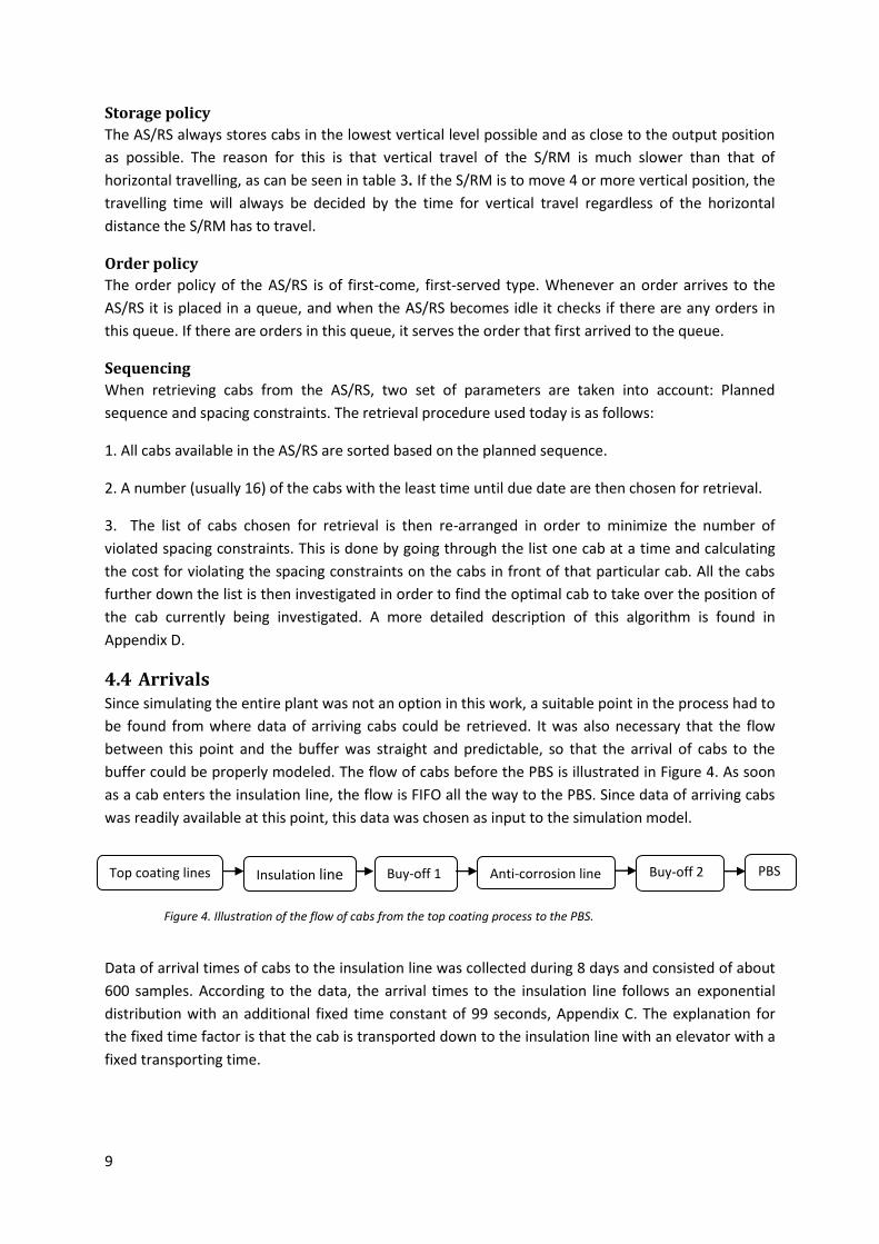
4.4 Arrivals Since simulating the entire plant was not an option in this work, a suitable point in the process had to

be found from where data of arriving cabs could be retrieved. It was also necessary that the flow

between this point and the buffer was straight and predictable, so that the arrival of cabs to the

buffer could be properly modeled. The flow of cabs before the PBS is illustrated in Figure 4. As soon

as a cab enters the insulation line, the flow is FIFO all the way to the PBS. Since data of arriving cabs

was readily available at this point, this data was chosen as input to the simulation model.

Data of arrival times of cabs to the insulation line was collected during 8 days and consisted of about

600 samples. According to the data, the arrival times to the insulation line follows an exponential

distribution with an additional fixed time constant of 99 seconds, Appendix C. The explanation for

the fixed time factor is that the cab is transported down to the insulation line with an elevator with a

fixed transporting time.

Insulation line Anti-corrosion line Top coating lines Buy-off 2 Buy-off 1

Figure 4. Illustration of the flow of cabs from the top coating process to the PBS.

PBS

10

-800 -600 -400 -200 0 200 4000

200

400

600

800

1000

1200

Sequence deviation (positions from planned sequence)

Num

ber

of

cabs

-800 -600 -400 -200 0 200 4000

200

400

600

800

1000

1200

Sequence deviation (positions from planned sequence)

Num

ber

of

cabs

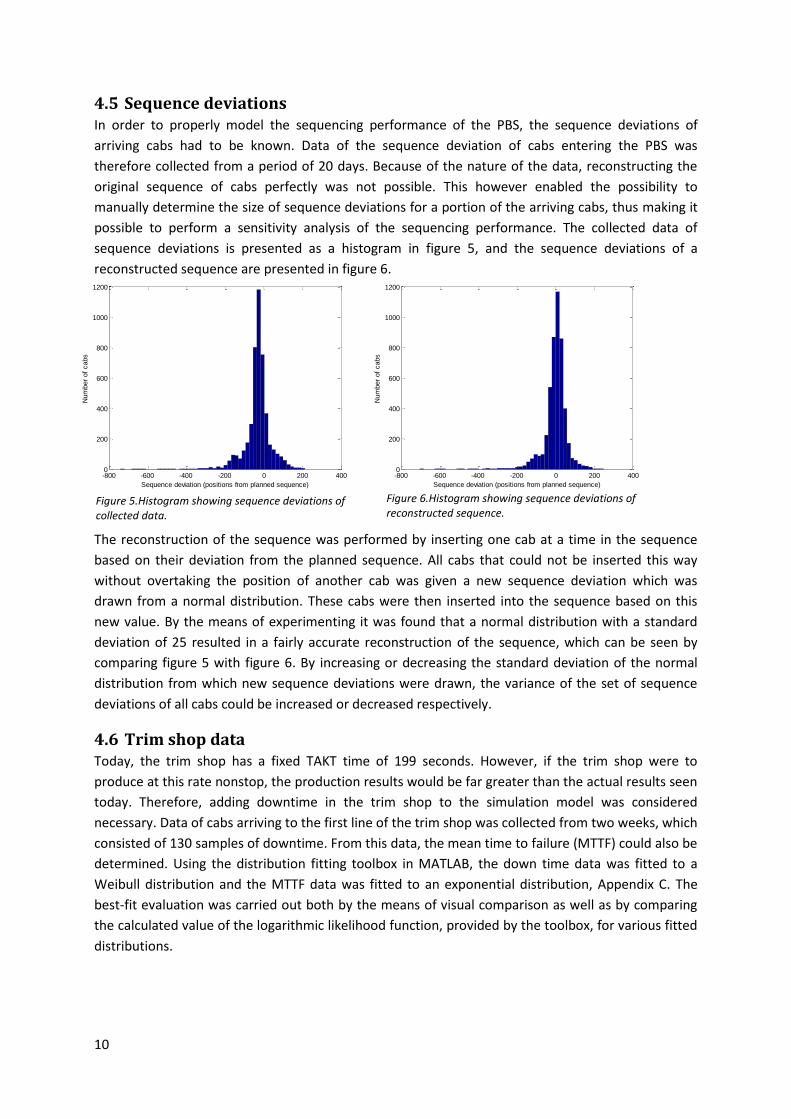
4.5 Sequence deviations In order to properly model the sequencing performance of the PBS, the sequence deviations of

arriving cabs had to be known. Data of the sequence deviation of cabs entering the PBS was

therefore collected from a period of 20 days. Because of the nature of the data, reconstructing the

original sequence of cabs perfectly was not possible. This however enabled the possibility to

manually determine the size of sequence deviations for a portion of the arriving cabs, thus making it

possible to perform a sensitivity analysis of the sequencing performance. The collected data of

sequence deviations is presented as a histogram in figure 5, and the sequence deviations of a

reconstructed sequence are presented in figure 6.

The reconstruction of the sequence was performed by inserting one cab at a time in the sequence

based on their deviation from the planned sequence. All cabs that could not be inserted this way

without overtaking the position of another cab was given a new sequence deviation which was

drawn from a normal distribution. These cabs were then inserted into the sequence based on this

new value. By the means of experimenting it was found that a normal distribution with a standard

deviation of 25 resulted in a fairly accurate reconstruction of the sequence, which can be seen by

comparing figure 5 with figure 6. By increasing or decreasing the standard deviation of the normal

distribution from which new sequence deviations were drawn, the variance of the set of sequence

deviations of all cabs could be increased or decreased respectively.

4.6 Trim shop data Today, the trim shop has a fixed TAKT time of 199 seconds. However, if the trim shop were to

produce at this rate nonstop, the production results would be far greater than the actual results seen

today. Therefore, adding downtime in the trim shop to the simulation model was considered

necessary. Data of cabs arriving to the first line of the trim shop was collected from two weeks, which

consisted of 130 samples of downtime. From this data, the mean time to failure (MTTF) could also be

determined. Using the distribution fitting toolbox in MATLAB, the down time data was fitted to a

Weibull distribution and the MTTF data was fitted to an exponential distribution, Appendix C. The

best-fit evaluation was carried out both by the means of visual comparison as well as by comparing

the calculated value of the logarithmic likelihood function, provided by the toolbox, for various fitted

distributions.

Figure 5.Histogram showing sequence deviations of collected data.

Figure 6.Histogram showing sequence deviations of reconstructed sequence.

11

4.7 Production Schedule The trim shop is operated in two shifts while the shops in the base process are operated in three.

Also, all shops have different working schedules for different days of the week. The result of this is

that up to ten percent more cabs than the average production rate are produced on a day with the

most working hours. In order to simulate the maximum load on the PBS, the working schedule of

Mondays was chosen to be used in simulation, both for the paint shop and trim shop, Appendix B.

Because of the low manpower during the night shift, the TAKT time during the day is different from

the TAKT time during the night. However, the planning department has defined production goals,

specifying that 216 cabs should be produced on Mondays during the day shifts and 44 during the

night shift, resulting in a total of 260 cabs.

If the night shift in the paint shop was to be fully manned, and the TAKT time during the night equal

to the TAKT time during the day, a weekly average production rate of 280 cabs / day would be

possible. This is also the specified maximum capacity of the plant today.

In the trim shop, the weekly average production rate is only 235 cabs / day. The difference between

the production rate of the paint shop and the trim shop is caused by some cabs not entering the trim

shop, for example cabs destined for special assembly. Approximately 3.3 percent of the cabs

produced in the paint shop never enter the trim shop. These cabs exit the paint shop right before the

point where cabs are transported to the PBS.

The Monday production goal in the trim shop is 254 cabs which based on the effective working time

would result in a mean production time of 212 seconds. However, because of downtime in the

process, the fixed TAKT time in the trim shop is set to 199 seconds. Since the actual production

results sometimes exceeds the production goals, the production rate that the PBS has to be able to

handle in simulations was defined as 10 % more than the average production rate.

12

5. Throughput analysis The first part of the analysis focuses on the throughput of the PBS. As a first step, the performance of

the existing system is investigated. Solutions are then presented and analyzed step by step for the

investigated production rates. In the second part, an analytical approach is used to investigate the

capacity requirements of the PBS for different production rates.

5.1 Performance analysis of the AS/RS The first step in the analysis was to determine the maximum performance of the existing system. In

order to do so, a model of the AS/RS was first implemented in MATLAB.

The store and retrieval policies, as well as the travelling times of the S/RM and the times for picking

and storing a cab was modeled as described in chapter 3.3. The production rate of today was then

simulated with the buffer level initiated to 90 % of maximum capacity. Simulations showed that the

cycle time of the S/RM followed a normal distribution with a mean cycle time of 93.5 seconds and a

standard deviation of 10 seconds. According to the maintenance department, the average cycle time

of the S/RM is 1.5 minutes, which indicates the validity of the model.

By knowing the cycle time of the S/RM, it is possible to calculate the maximum number of cabs that

the AS/RS can handle during one day of production. The theoretical maximum production rate can

then be approximated by taking into account the production schedule as well as the difference in

production pace during the day and night shift, as stated in 3.7.

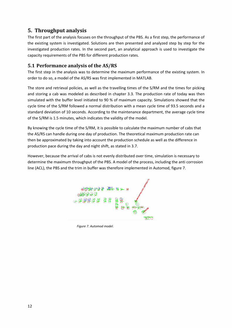
However, because the arrival of cabs is not evenly distributed over time, simulation is necessary to

determine the maximum throughput of the PBS. A model of the process, including the anti corrosion

line (ACL), the PBS and the trim in buffer was therefore implemented in Automod, figure 7.

Figure 7. Automod model.

13

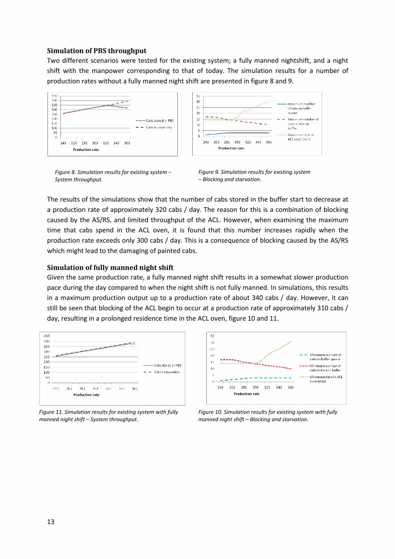
Simulation of PBS throughput

Two different scenarios were tested for the existing system; a fully manned nightshift, and a night

shift with the manpower corresponding to that of today. The simulation results for a number of

production rates without a fully manned night shift are presented in figure 8 and 9.

The results of the simulations show that the number of cabs stored in the buffer start to decrease at

a production rate of approximately 320 cabs / day. The reason for this is a combination of blocking

caused by the AS/RS, and limited throughput of the ACL. However, when examining the maximum

time that cabs spend in the ACL oven, it is found that this number increases rapidly when the

production rate exceeds only 300 cabs / day. This is a consequence of blocking caused by the AS/RS

which might lead to the damaging of painted cabs.

Simulation of fully manned night shift

Given the same production rate, a fully manned night shift results in a somewhat slower production

pace during the day compared to when the night shift is not fully manned. In simulations, this results

in a maximum production output up to a production rate of about 340 cabs / day. However, it can

still be seen that blocking of the ACL begin to occur at a production rate of approximately 310 cabs /

day, resulting in a prolonged residence time in the ACL oven, figure 10 and 11.

Figure 8. Simulation results for existing system – System throughput.

Figure 9. Simulation results for existing system – Blocking and starvation.

Figure 11. Simulation results for existing system with fully manned night shift – System throughput.

Figure 10. Simulation results for existing system with fully manned night shift – Blocking and starvation.

14

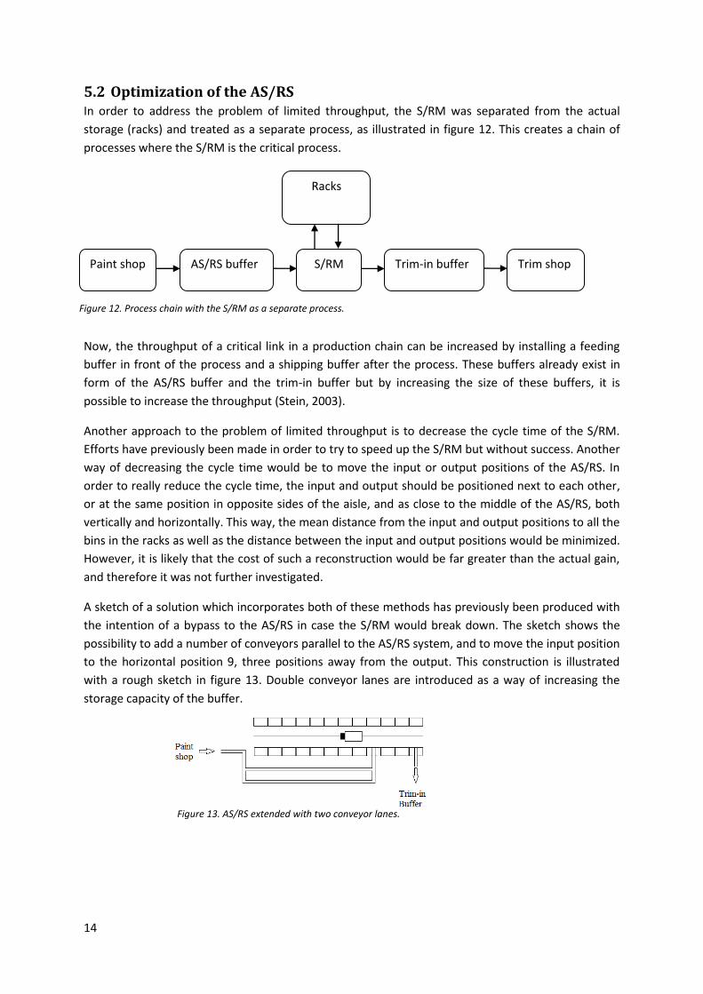
5.2 Optimization of the AS/RS In order to address the problem of limited throughput, the S/RM was separated from the actual

storage (racks) and treated as a separate process, as illustrated in figure 12. This creates a chain of

processes where the S/RM is the critical process.

Now, the throughput of a critical link in a production chain can be increased by installing a feeding

buffer in front of the process and a shipping buffer after the process. These buffers already exist in

form of the AS/RS buffer and the trim-in buffer but by increasing the size of these buffers, it is

possible to increase the throughput (Stein, 2003).

Another approach to the problem of limited throughput is to decrease the cycle time of the S/RM.

Efforts have previously been made in order to try to speed up the S/RM but without success. Another

way of decreasing the cycle time would be to move the input or output positions of the AS/RS. In

order to really reduce the cycle time, the input and output should be positioned next to each other,

or at the same position in opposite sides of the aisle, and as close to the middle of the AS/RS, both

vertically and horizontally. This way, the mean distance from the input and output positions to all the

bins in the racks as well as the distance between the input and output positions would be minimized.

However, it is likely that the cost of such a reconstruction would be far greater than the actual gain,

and therefore it was not further investigated.

A sketch of a solution which incorporates both of these methods has previously been produced with

the intention of a bypass to the AS/RS in case the S/RM would break down. The sketch shows the

possibility to add a number of conveyors parallel to the AS/RS system, and to move the input position

to the horizontal position 9, three positions away from the output. This construction is illustrated

with a rough sketch in figure 13. Double conveyor lanes are introduced as a way of increasing the

storage capacity of the buffer.

Paint shop S/RM

Racks

AS/RS buffer Trim-in buffer Trim shop

Figure 13. AS/RS extended with two conveyor lanes.

Figure 12. Process chain with the S/RM as a separate process.

15

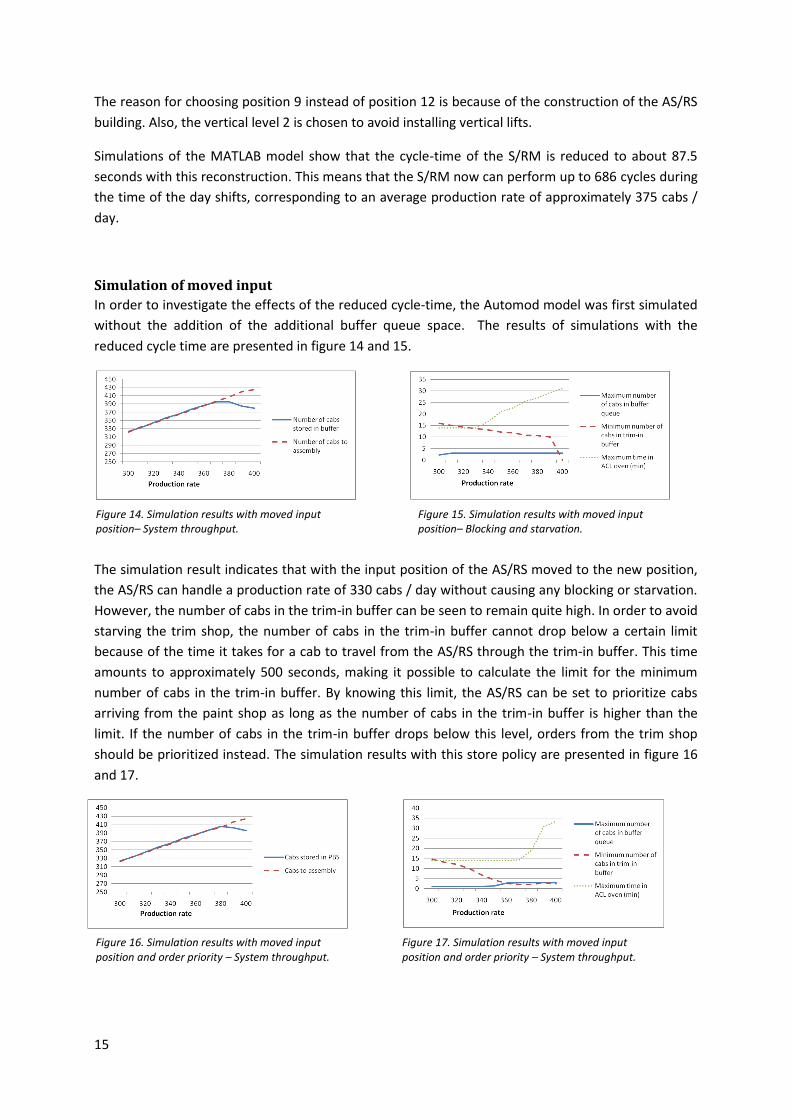
The reason for choosing position 9 instead of position 12 is because of the construction of the AS/RS

building. Also, the vertical level 2 is chosen to avoid installing vertical lifts.

Simulations of the MATLAB model show that the cycle-time of the S/RM is reduced to about 87.5

seconds with this reconstruction. This means that the S/RM now can perform up to 686 cycles during

the time of the day shifts, corresponding to an average production rate of approximately 375 cabs /

day.

Simulation of moved input

In order to investigate the effects of the reduced cycle-time, the Automod model was first simulated

without the addition of the additional buffer queue space. The results of simulations with the

reduced cycle time are presented in figure 14 and 15.

The simulation result indicates that with the input position of the AS/RS moved to the new position,

the AS/RS can handle a production rate of 330 cabs / day without causing any blocking or starvation.

However, the number of cabs in the trim-in buffer can be seen to remain quite high. In order to avoid

starving the trim shop, the number of cabs in the trim-in buffer cannot drop below a certain limit

because of the time it takes for a cab to travel from the AS/RS through the trim-in buffer. This time

amounts to approximately 500 seconds, making it possible to calculate the limit for the minimum

number of cabs in the trim-in buffer. By knowing this limit, the AS/RS can be set to prioritize cabs

arriving from the paint shop as long as the number of cabs in the trim-in buffer is higher than the

limit. If the number of cabs in the trim-in buffer drops below this level, orders from the trim shop

should be prioritized instead. The simulation results with this store policy are presented in figure 16

and 17.

Figure 16. Simulation results with moved input position and order priority – System throughput.

Figure 17. Simulation results with moved input position and order priority – System throughput.

Figure 14. Simulation results with moved input position– System throughput.

Figure 15. Simulation results with moved input position– Blocking and starvation.

16

These results show that with the input position moved to the new location, and with this new store

policy, a production rate of 370 cabs / day can be handled without adding extra positions to the

buffer queue or trim-in buffer. This means that all the added extra space in the buffer queue can be

used as extra buffer space, instead of having to be free in order to accumulate blocking caused by the

PBS.

5.3 Parallel selectivity bank If the production rate is to be further increased to levels up to 410 or even 490 cabs / day, the single

AS/RS alone will not be able to achieve necessary throughput without significant modifications. Also,

which will be discussed in section 5, the size of the buffer will have to be significantly increased.

Obvious solutions to these problems would be to either construct a new parallel AS/RS, or expand

the current system with a new aisle and S/RM. However, such constructions are very expensive,

mainly due to the large building required.

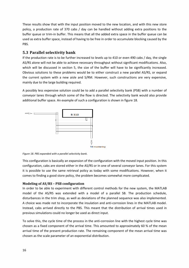
A possibly less expensive solution could be to add a parallel selectivity bank (PSB) with a number of

conveyor lanes through which some of the flow is directed. The selectivity bank would also provide

additional buffer space. An example of such a configuration is shown in figure 18.

Figure 18. PBS expanded with a parallel selectivity bank.

This configuration is basically an expansion of the configuration with the moved input position. In this

configuration, cabs are stored either in the AS/RS or in one of several conveyor lanes. For this system

it is possible to use the same retrieval policy as today with some modifications. However, when it

comes to finding a good store policy, the problem becomes somewhat more complicated.

Modeling of AS/RS – PSB configuration

In order to be able to experiment with different control methods for the new system, the MATLAB

model of the AS/RS was extended with a model of a parallel SB. The production schedule,

disturbances in the trim shop, as well as deviations of the planned sequence was also implemented.

A choice was made not to incorporate the insulation and anti-corrosion lines in the MATLAB model.

Instead, cabs arrived directly to the PBS. This meant that the distribution of arrival times used in

previous simulations could no longer be used as direct input.

To solve this, the cycle time of the process in the anti-corrosion line with the highest cycle time was

chosen as a fixed component of the arrival time. This amounted to approximately 60 % of the mean

arrival time of the present production rate. The remaining component of the mean arrival time was

chosen as the scale parameter of an exponential distribution.

17

The model was validated without the PSB to make sure that the output of simulations in terms of

throughput and correctness of sequence of cabs sent to the trim shop corresponded to the company

data. It was then simulated with different sizes of the PSB, and different policies for storage and

retrieval was evaluated.

Retrieval policy

The retrieval policy has two main objectives:

Minimize violations of spacing constraints

Minimize deviations of the planned sequence

Both of these objectives were handled well by the currently used retrieval policy, and thus, it was

decided that this policy was to be used in the new system. However some modifications had to be

done to the old retrieval policy. The main difference now was that it had to be assured that the order

in which cabs were retrieved from the selectivity bank would not be in conflict with the order in

which they were arranged in the conveyor lanes.

The new retrieval policy can be described as follows:

1. All cabs that are stored in the AS/RS are placed in a list and then sorted in order of planned

sequence.

2. Each cab in the selectivity bank is inserted in the list based on their planned sequence, but not

higher than cabs positioned ahead on the same conveyor lane.

3. A number of N cabs positioned highest in the list are then chosen for retrieval.

4. The list of cabs chosen for retrieval is then re-arranged using the same algorithm as before with

the addition of one extra step, see Algorithm 1, Appendix D.

Store policy

The two main objectives of the store policy is to:

Minimize deviations from the planned sequence by storing an arriving cab in an appropriate

position.

Minimize the flow of cabs through the AS/RS.

From experiments with the simulation model it could be seen that the location of cabs in the

selectivity bank were relatively unimportant for attaining few constraint violations. However, if the

deviations from the planned sequence were to be minimized, the location of cabs in the selectivity

bank is critical. For example, if a cab which is already late for assembly is positioned behind a cab

which has arrived early in a conveyor lane, the cab which is already late will become ever more so.

Besides minimizing deviations from the planned sequence, a large part of the flow of cabs had to be

directed through the selectivity bank. If the flow through the AS/RS becomes too large, significant

blocking of the ACL line or starvation of the trim shop might occur.

The main problem when trying to find a good store policy which handles both of these objectives is

the large variations in the arriving cabs deviations from the planned sequence. This results in that the

two objectives becomes very much in conflict with each other.

18

0 10 20 30 40 50 60 70 800

20

40

60

80

100

120

140

160

Time (h)

Num

ber

of

cabs

Cabs in AS/RS

Cabs in queue

Cabs in SB

Choice of conveyor lane

Before the decision is made of whether to store an arriving cab in the AS/RS or the selectivity bank,

the selectivity bank is investigated in order to find the most suitable conveyor lane in which to store

the arriving cab. The method which was used was to calculate a cost based on the difference in

planned sequence between the arriving cab and the cabs at the rear of each conveyor lane. A more

detailed description is found in Appendix D.

Choice of storage system

With the goal of fulfilling both of the two main objectives of the store policy, a number of different

methods for deciding where to store arriving cabs was created and tested. When evaluating the

different methods, one very simple approach seemed to be quite effective. This method looks at the

cost calculated when searching for the best suited conveyor lane. It then specifies that if this cost is

less than a predefined limit ( ), then the arriving cab can be stored in the selected lane in the

selectivity bank.

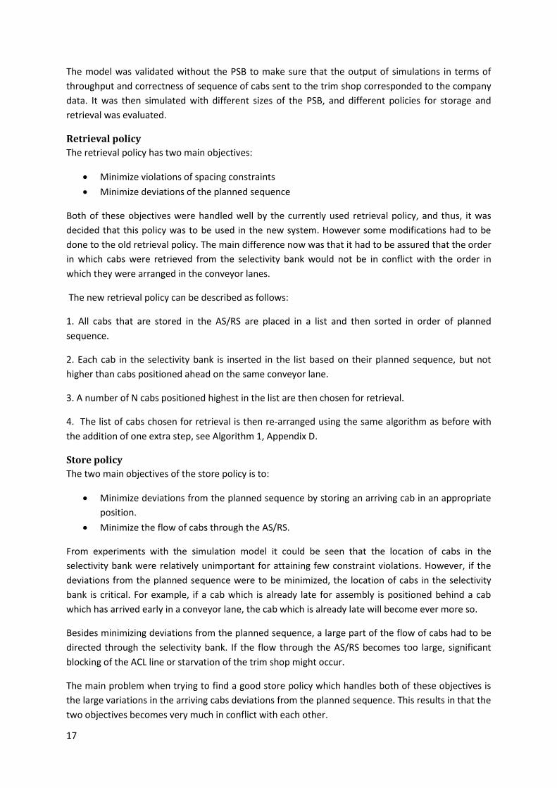
Simulation of AS/RS – PSB configuration

The buffer levels during a three day simulation of a production rate of 410 cabs / day, and with a

4*10 selectivity bank, using the described policies are presented in figure 19.

During the simulation, queue build up can be seen to occur at a few occasions. One of the reasons for

this is that is fixed. Because of the large variations of the sequence deviations of arriving cabs, the

fixed value of results in that there are times when very few cabs are stored in the SB. Another

reason is that most cabs during the night shift are stored in the AS/RS. Generally, most of these cabs

are scheduled within a confined sequence window, resulting in a large number of consecutive cabs

being retrieved from the AS/RS during a period of time the next day. Even if many cabs are stored in

the selectivity bank during this period, the selectivity bank will eventually fill up, with the

consequence of blocking the ACL line.

The solution to this problem is to keep the number of cabs in the selectivity bank relatively low

during the day so that it can be filled up during the night. In order to do so and still handle the main

objectives, a new control method was developed. This method seeks to keep the number of cabs in

the selectivity bank as close to a predefined number as possible during the day by constantly

adjusting the value of the cost limit based on the flow of cabs. The control method is explained in

more detail in Appendix D.

Figure 19. Simulation results with the PBS expanded with a 4*10 selectivity bank using a fixed-limit control method for a production rate of 410 cabs / day.

19

0 10 20 30 40 50 60 70 800

20

40

60

80

100

120

140

160

Time (h)N

um

ber

of

cabs

Cabs in AS/RS

Cabs in queue

Cabs in SB

0 10 20 30 40 50 60 70 800

20

40

60

80

100

120

140

160

Time (h)

Num

ber

of

cabs

Cabs in AS/RS

Cabs in queue

Cabs in SB

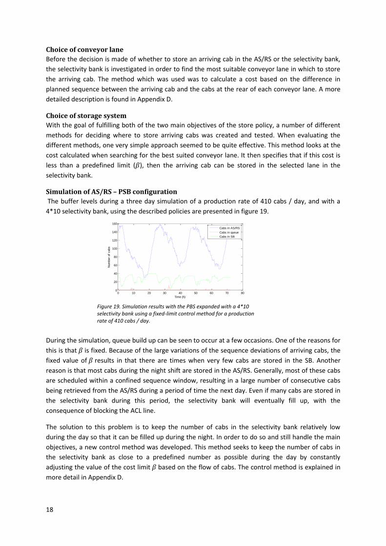
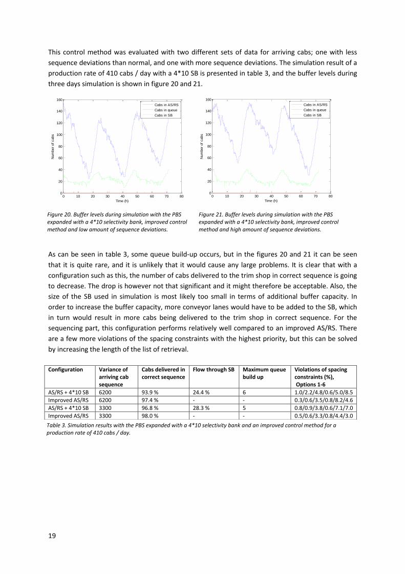
This control method was evaluated with two different sets of data for arriving cabs; one with less

sequence deviations than normal, and one with more sequence deviations. The simulation result of a

production rate of 410 cabs / day with a 4*10 SB is presented in table 3, and the buffer levels during

three days simulation is shown in figure 20 and 21.

As can be seen in table 3, some queue build-up occurs, but in the figures 20 and 21 it can be seen

that it is quite rare, and it is unlikely that it would cause any large problems. It is clear that with a

configuration such as this, the number of cabs delivered to the trim shop in correct sequence is going

to decrease. The drop is however not that significant and it might therefore be acceptable. Also, the

size of the SB used in simulation is most likely too small in terms of additional buffer capacity. In

order to increase the buffer capacity, more conveyor lanes would have to be added to the SB, which

in turn would result in more cabs being delivered to the trim shop in correct sequence. For the

sequencing part, this configuration performs relatively well compared to an improved AS/RS. There

are a few more violations of the spacing constraints with the highest priority, but this can be solved

by increasing the length of the list of retrieval.

Configuration Variance of arriving cab sequence

Cabs delivered in correct sequence

Flow through SB Maximum queue build up

Violations of spacing constraints (%), Options 1-6

AS/RS + 4*10 SB 6200 93.9 % 24.4 % 6 1.0/2.2/4.8/0.6/5.0/8.5

Improved AS/RS 6200 97.4 % - - 0.3/0.6/3.5/0.8/8.2/4.6

AS/RS + 4*10 SB 3300 96.8 % 28.3 % 5 0.8/0.9/3.8/0.6/7.1/7.0

Improved AS/RS 3300 98.0 % - - 0.5/0.6/3.3/0.8/4.4/3.0

Table 3. Simulation results with the PBS expanded with a 4*10 selectivity bank and an improved control method for a production rate of 410 cabs / day.

Figure 20. Buffer levels during simulation with the PBS expanded with a 4*10 selectivity bank, improved control method and low amount of sequence deviations.

Figure 21. Buffer levels during simulation with the PBS expanded with a 4*10 selectivity bank, improved control method and high amount of sequence deviations.

20

0 10 20 30 40 50 60 70 800

20

40

60

80

100

120

140

Time (h)

Num

ber

of

cabs

Cabs in AS/RS

Cabs in queue

Cabs in SB

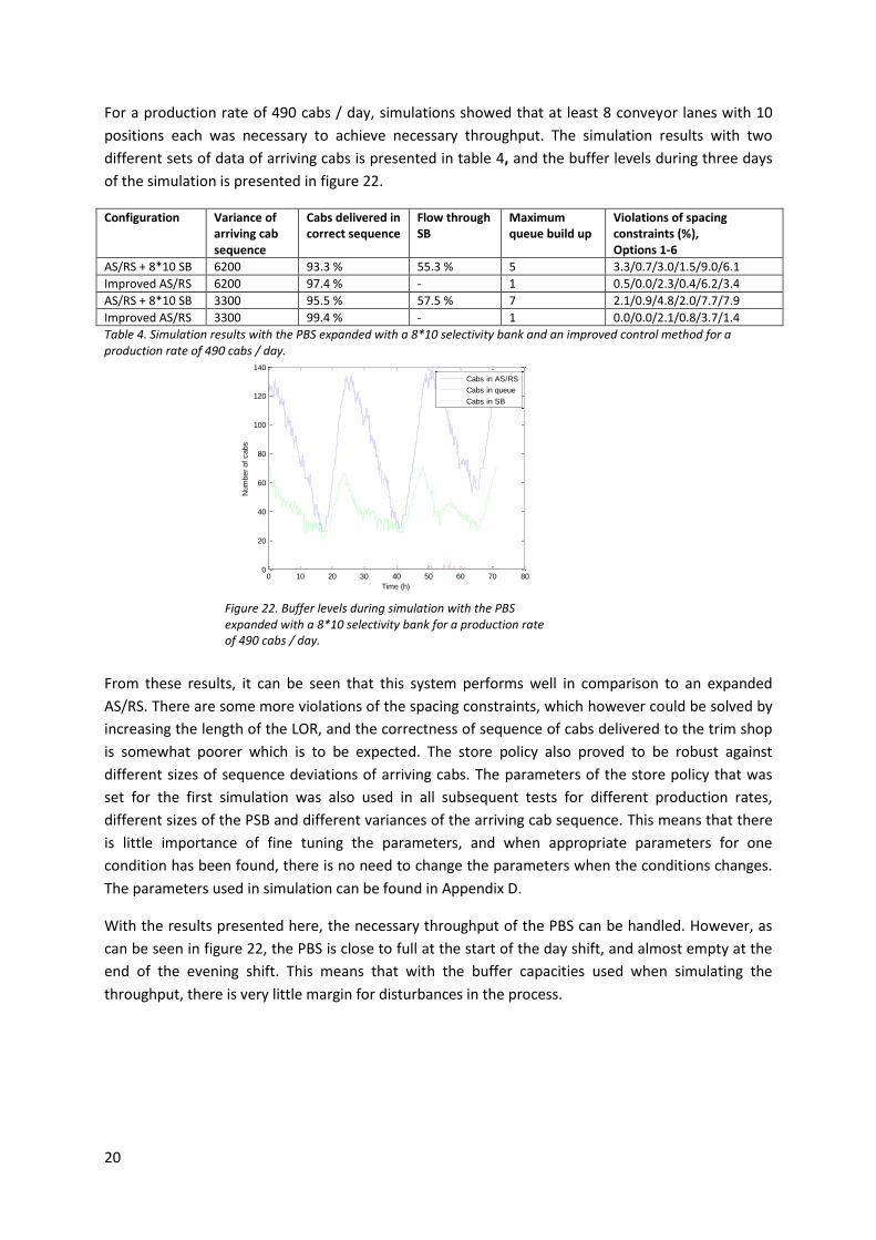
For a production rate of 490 cabs / day, simulations showed that at least 8 conveyor lanes with 10

positions each was necessary to achieve necessary throughput. The simulation results with two

different sets of data of arriving cabs is presented in table 4, and the buffer levels during three days

of the simulation is presented in figure 22.

Configuration Variance of arriving cab sequence

Cabs delivered in correct sequence

Flow through SB

Maximum queue build up

Violations of spacing constraints (%), Options 1-6

AS/RS + 8*10 SB 6200 93.3 % 55.3 % 5 3.3/0.7/3.0/1.5/9.0/6.1

Improved AS/RS 6200 97.4 % - 1 0.5/0.0/2.3/0.4/6.2/3.4

AS/RS + 8*10 SB 3300 95.5 % 57.5 % 7 2.1/0.9/4.8/2.0/7.7/7.9

Improved AS/RS 3300 99.4 % - 1 0.0/0.0/2.1/0.8/3.7/1.4

Table 4. Simulation results with the PBS expanded with a 8*10 selectivity bank and an improved control method for a production rate of 490 cabs / day.

From these results, it can be seen that this system performs well in comparison to an expanded

AS/RS. There are some more violations of the spacing constraints, which however could be solved by

increasing the length of the LOR, and the correctness of sequence of cabs delivered to the trim shop

is somewhat poorer which is to be expected. The store policy also proved to be robust against

different sizes of sequence deviations of arriving cabs. The parameters of the store policy that was

set for the first simulation was also used in all subsequent tests for different production rates,

different sizes of the PSB and different variances of the arriving cab sequence. This means that there

is little importance of fine tuning the parameters, and when appropriate parameters for one

condition has been found, there is no need to change the parameters when the conditions changes.

The parameters used in simulation can be found in Appendix D.

With the results presented here, the necessary throughput of the PBS can be handled. However, as

can be seen in figure 22, the PBS is close to full at the start of the day shift, and almost empty at the

end of the evening shift. This means that with the buffer capacities used when simulating the

throughput, there is very little margin for disturbances in the process.

Figure 22. Buffer levels during simulation with the PBS expanded with a 8*10 selectivity bank for a production rate of 490 cabs / day.

21

6. Buffer capacity The PBS in focus in this thesis has three main objectives; Handle the different working hours in the

paint shop and trim shop, handle disturbances in the process, and restore the planned sequence of

cabs. It also has a fourth objective which is to handle the lead times for material logistics in the trim

shop.

The demands on necessary buffer space that follows from the first objective can be derived by simply

calculating the number of cabs that is to be produced in the paint shop during the night. With the

working schedules used today, and with a fully manned night shift, this amount to approximately 28

% of all cabs produced during one day.

When investigating the need of buffer space to handle disturbances, all factors which affect the

buffer level of the PBS has to be taken into account. Some of these are:

Downtimes and low utilization of resources in the paint shop.

Cabs having to be repaired or repainted.

Very few or very many of the painted cabs are sent to other destinations, for example special

assembly, and thus not entering the PBS.

More or less stop time than normal in the assembly lines.

Disturbances earlier in the process, for example in the body shop or primer process.

Active decisions taken by the management, for example overtime.

6.1 Difficulties with simulation When determining appropriate buffer space for an in-process buffer, simulation is often a valuable

tool. However, there are some cases when simulation is not appropriate. For example when the

system behavior is too complex or cannot be defined, the model cannot be validated, or when the

problem can be solved analytically (Nelson, Banks, & Nicol, 2000). In some ways, simulation of the

PBS relate to all three of these situations.

For the production rates of 410 and 490 cabs / day, it is unknown what modifications will have to be

made in the process and what effect these modifications will have. This of course makes it difficult to

validate any models of these scenarios, but it might still be possible to simulate such scenarios by

making reasonable assumptions.

The main problem however when trying to investigate the necessary buffer capacity is that the

buffer level is highly influenced by operative decisions made by the management. In the real world,

the reason for any larger disturbance in the process is generally known. This means that decision of

countermeasures, i.e. overtime, can be taken based on knowledge of the disturbance. For example, if

a robot breaks down on the main paint line it is possible to predict the size of the disturbance (time

before the robot is fixed) and take appropriate countermeasures in order to reduce the effect of the

disturbance.

In simulations on the other hand, disturbances are generated by random numbers without any

underlying cause. This means that rules for calling overtime can only be defined based on the

simulation outcome.

22

6.2 Buffer levels Today, the specified normal buffer level after the night shift, including the trim-in buffers 19

positions, is specified to 140-175 cabs. If the buffer level drops below 140, a decision is taken of

whether to call overtime in the paint shop. The reason for this level being so high is because of the

large sequence deviations of cabs leaving the paint shop, but as a consequence, the trim shop rarely

experience starvation.

If the upper buffer limit is exceeded, cabs can be transported to an external storage area located

outside the factory building for temporary storage. However, because the cabs have to be taken out

of the building and transported by truck to this storage area, this is not considered to be an optimal

solution. Also, when the upper buffer limit is reached, it is up to the management to decide if the

extra storage area should be used or if production should be stopped.

Some buffer space in the in-house buffer is always left empty in case cabs that are late for assembly

were to arrive from the paint shop.

6.3 Statistical analysis With the assumption that the availability of all resources in the process will remain the same in the

future, it is possible to approximate the necessary buffer capacity of future production rates by

determining necessary buffer space for the current production rate. In order to do so, two different

approaches were used;

Observed buffer levels

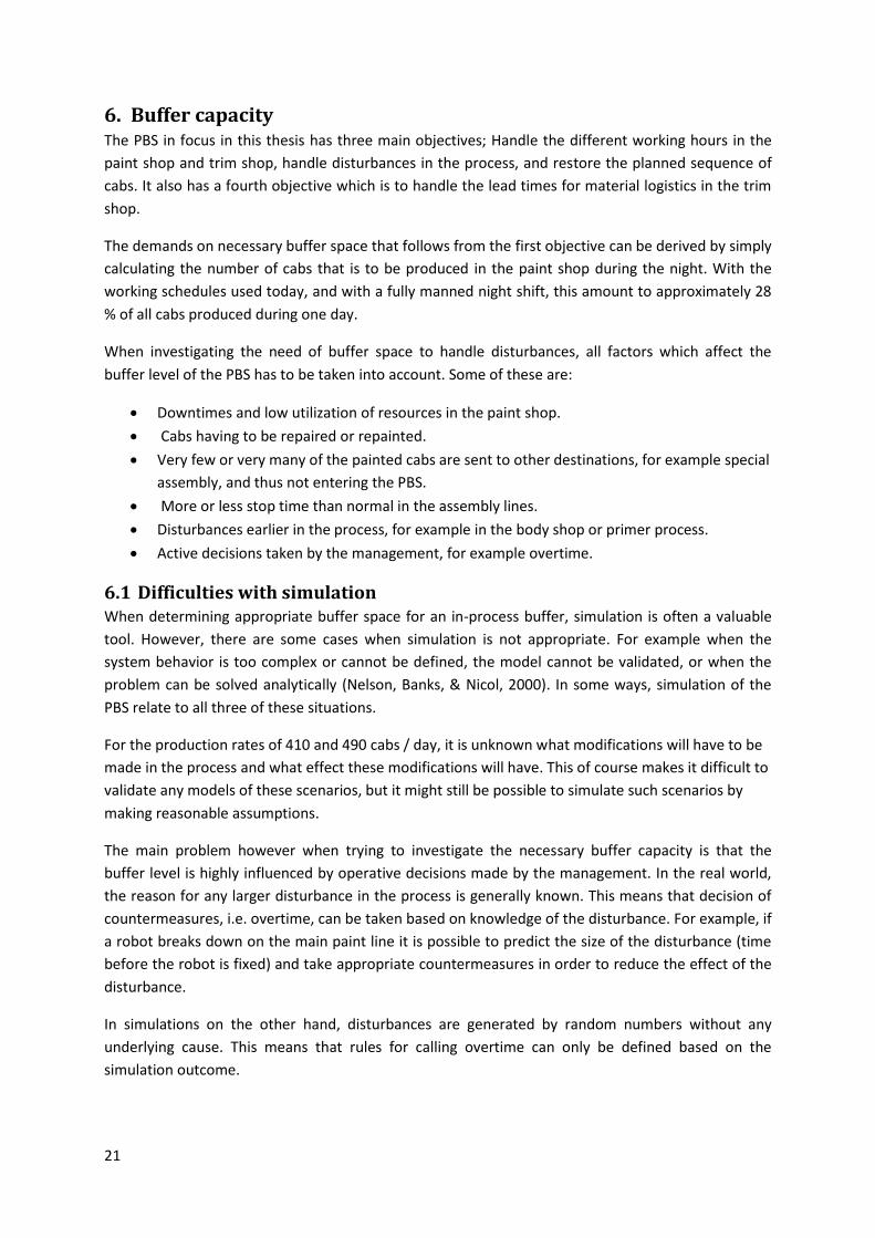
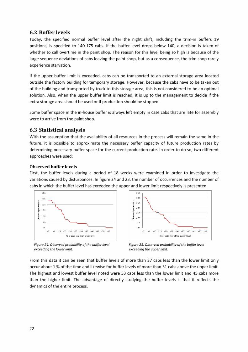
First, the buffer levels during a period of 18 weeks were examined in order to investigate the

variations caused by disturbances. In figure 24 and 23, the number of occurrences and the number of

cabs in which the buffer level has exceeded the upper and lower limit respectively is presented.

From this data it can be seen that buffer levels of more than 37 cabs less than the lower limit only

occur about 1 % of the time and likewise for buffer levels of more than 31 cabs above the upper limit.

The highest and lowest buffer level noted were 53 cabs less than the lower limit and 45 cabs more

than the higher limit. The advantage of directly studying the buffer levels is that it reflects the

dynamics of the entire process.

Figure 24. Observed probability of the buffer level exceeding the lower limit.

Figure 23. Observed probability of the buffer level exceeding the upper limit.

23

Disturbance probability

The goal with the second approach was to calculate the probability of buffer level variations of

different sizes based on statistics of production outcome.

Data of the achieved production result in percentage of the planned production goals was collected

from a period of five months. These data were then fitted to a normal and Weibull distribution for

the paint shop and trim shop respectively. With these distributions, the probability that a buffer level

variation is larger than a given value could be calculated, see Appendix E.

However, in order to determine necessary buffer space to handle disturbances, it is necessary to also

look at variations over a period of two days. The reason for this is that one days notice is needed in

order to call overtime.

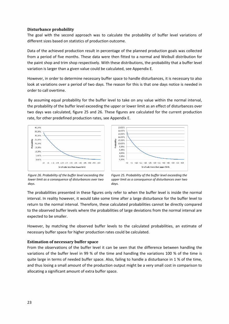
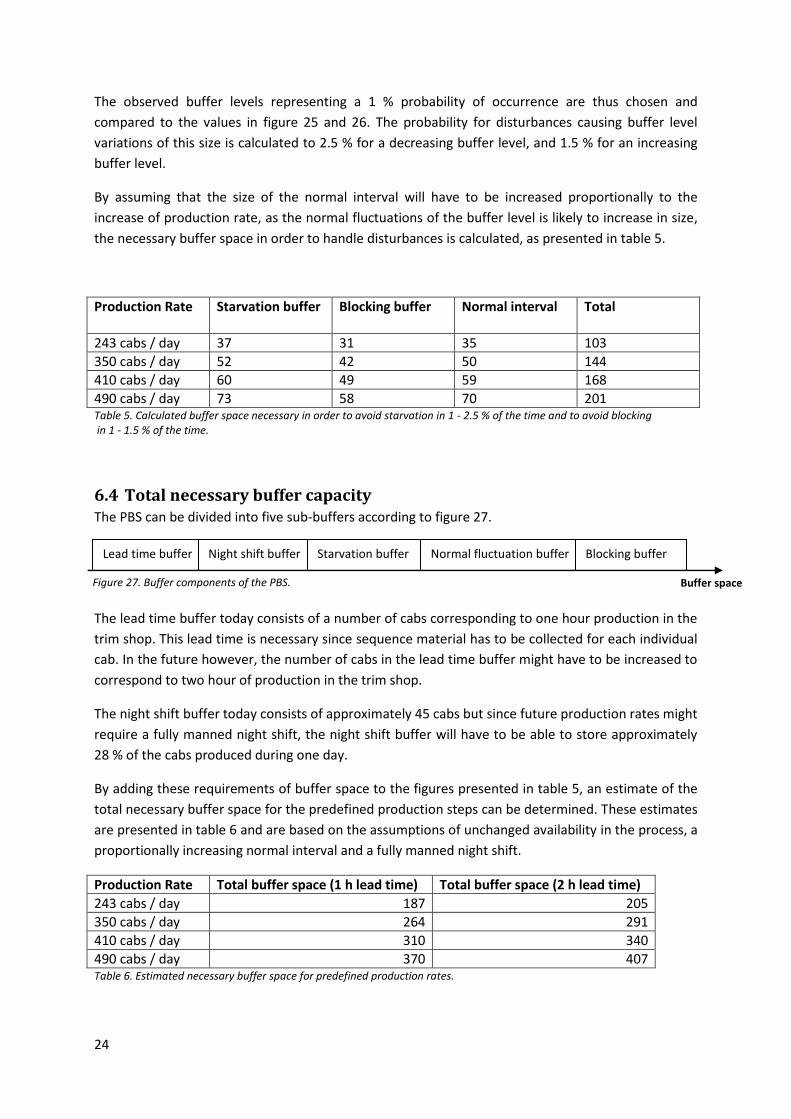
By assuming equal probability for the buffer level to take on any value within the normal interval,

the probability of the buffer level exceeding the upper or lower limit as an effect of disturbances over

two days was calculated, figure 25 and 26. These figures are calculated for the current production

rate, for other predefined production rates, see Appendix E.

The probabilities presented in these figures only refer to when the buffer level is inside the normal

interval. In reality however, it would take some time after a large disturbance for the buffer level to

return to the normal interval. Therefore, these calculated probabilities cannot be directly compared

to the observed buffer levels where the probabilities of large deviations from the normal interval are

expected to be smaller.

However, by matching the observed buffer levels to the calculated probabilities, an estimate of

necessary buffer space for higher production rates could be calculated.

Estimation of necessary buffer space

From the observations of the buffer level it can be seen that the difference between handling the

variations of the buffer level in 99 % of the time and handling the variations 100 % of the time is

quite large in terms of needed buffer space. Also, failing to handle a disturbance in 1 % of the time,

and thus losing a small amount of the production output might be a very small cost in comparison to

allocating a significant amount of extra buffer space.

Figure 26. Probability of the buffer level exceeding the lower limit as a consequence of disturbances over two days.

Figure 25. Probability of the buffer level exceeding the upper limit as a consequence of disturbances over two days.

24

The observed buffer levels representing a 1 % probability of occurrence are thus chosen and

compared to the values in figure 25 and 26. The probability for disturbances causing buffer level

variations of this size is calculated to 2.5 % for a decreasing buffer level, and 1.5 % for an increasing

buffer level.

By assuming that the size of the normal interval will have to be increased proportionally to the

increase of production rate, as the normal fluctuations of the buffer level is likely to increase in size,

the necessary buffer space in order to handle disturbances is calculated, as presented in table 5.

Production Rate Starvation buffer Blocking buffer

Normal interval Total

243 cabs / day 37 31 35 103

350 cabs / day 52 42 50 144

410 cabs / day 60 49 59 168

490 cabs / day 73 58 70 201 Table 5. Calculated buffer space necessary in order to avoid starvation in 1 - 2.5 % of the time and to avoid blocking in 1 - 1.5 % of the time.

6.4 Total necessary buffer capacity The PBS can be divided into five sub-buffers according to figure 27.

The lead time buffer today consists of a number of cabs corresponding to one hour production in the

trim shop. This lead time is necessary since sequence material has to be collected for each individual

cab. In the future however, the number of cabs in the lead time buffer might have to be increased to

correspond to two hour of production in the trim shop.

The night shift buffer today consists of approximately 45 cabs but since future production rates might

require a fully manned night shift, the night shift buffer will have to be able to store approximately

28 % of the cabs produced during one day.

By adding these requirements of buffer space to the figures presented in table 5, an estimate of the

total necessary buffer space for the predefined production steps can be determined. These estimates

are presented in table 6 and are based on the assumptions of unchanged availability in the process, a

proportionally increasing normal interval and a fully manned night shift.

Production Rate Total buffer space (1 h lead time) Total buffer space (2 h lead time)

243 cabs / day 187 205

350 cabs / day 264 291

410 cabs / day 310 340

490 cabs / day 370 407 Table 6. Estimated necessary buffer space for predefined production rates.

Buffer space

Lead time buffer Night shift buffer Starvation buffer Normal fluctuation buffer Blocking buffer

Figure 27. Buffer components of the PBS.

25

These calculations presented here are based solely on a statistical analysis. However, for

disturbances in the trim shop, it is not simply a question of the size of disturbances, but also a

question of how the plant is operated. Since Scania has a policy of client-driven production, one

might argue that the paint shop should stop producing if there no longer is a demand of cabs from

the trim shop. However, this might result in both the trim shop and the paint shop having to call

overtime, instead of just the trim shop. Still, based on operating principles it is possible to choose not

to incorporate (or reduce) the buffer space dedicated to handle disturbances in the trim shop, thus

reducing the total buffer space needed.

In the presented calculations of total necessary buffer space, no respect has been given to the

resequencing of cabs. This might cause problems at the end of the evening shift when the buffer

level is at its lowest point. If the paint shop has experienced disturbances, there might be very few

cabs in the buffer to choose between, resulting in a poor sequence to the trim shop. It might

therefore be of interest to consider allocating additional buffer space for this purpose. On the other

hand, in the event of large disturbances in the process, a poor sequence might be acceptable.

26

7. Conclusions It has been shown in this work that it is theoretically possible to increase the throughput of the PBS

without having to expand the current AS/RS, and that it is possible to do so in a number of steps in

which the throughput could be increased gradually to meet the production volume. It was also

shown that with the presented solutions, the sequencing performance, both in terms of minimizing

spacing constraints and following the planned sequence, would not be significantly reduced.

However, the main solution presented is based on storing cabs in conveyor lanes. The disadvantage

with such a storage system compared to an AS/RS is that the footprint becomes very large. And even

though the sizes needed for such a system in order to increase the throughput might be competitive

to expanding the current AS/RS, it is unlikely that it would be beneficial or even possible to construct

a conveyor based system large enough to provide enough buffer space for the predefined future

production volume of 490 cabs / day.

An example where a large 15-lane selectivity bank was chosen as PBS instead of an AS/RS can be

found at GM Holden (Kline Jr, 2000). The reason for choosing a selectivity bank in this example

however was mainly due to the fact that the building required to house the bank already existed, and

the objective of the PBS was not so much to provide buffer space as to provide high throughput and

sequencing possibilities.

In the final chapter, it was shown that given an unchanged availability in the process, a fully manned

night shift and with the operating procedure of today, a production rate of 490 cabs / day requires at

least that the amount of buffer space in the PBS is doubled.

27

8. Discussion The analysis of necessary buffer space showed that with the given assumptions, the buffer space

would have to be increased proportionally to an increase of the production rate. Approximately half

of the necessary buffer space follows from the demand of lead time and from the night shift in the

paint shop and can hardly be questioned.

The other half on the other side comes from the need to handle disturbances and is exposed to a

number of uncertainties. For example, both engineers and management at the company doubt that

the size of disturbances will increase proportional to the increased production rate. Also, the analysis

used a purely statistical approach where both the paint shop and trim shop were black-boxed. This

means that dynamics of the system was not taken into account. In order to be able to make a better

estimation of necessary buffer space, the change of size and frequency of disturbances in the process

for higher production rates should be investigated. Simulation of the entire process might be a good

way to achieve this.

Finally, before any decision is taken on expanding the PBS, an economical analysis of course has to be

performed. For example, the cost of creating extra buffer space should be weighed against the cost

of having to stop the production. As a support in this work, the calculated probabilities of the buffer

level exceeding the normal interval might be useful. These are presented in Appendix E for all

predefined production rates.

28

References Boysen, N., Scholl, A., & Woppere, N. (n.d.). Resequencing of Mixed-Model Assembly Lines: Survey

and Research Agenda.

Grinstead, C. M., & Snell, L. J. (1997). Introduction to Probability. United States of America: American

Mathematical Society.

Kline Jr, S. R. (2000, October). Maximizing Paint Shop Efficiency - GM Holden. Automotive Finishing .

Moon, D. H., Song, C., & Ha, J. H. (2005, November). A Dynamic Algorithm for the Control of

Automotive Painted Body Storage. SIMULATION , pp. 773-787.

Nelson, B. L., Banks, J., & Nicol, D. M. (2000). Discrete-event system simulation. Prentice Hall.

Ribeiro, L., Barata, J., & Sousa, P. (2009). An Algorithm for Management of Automotive Buffers with

Drawers. 2009 IEEE International Symposium on Assembly and Manufacturing , Suwon, Korea.

Scaniakoncernen. (2011, 05 19). Retrieved from http://www.scania.se/om-scania/scaniakoncernen/

Stein, E. R. (2003). Re-Engineering the manufacturing system - Applying the theory of constraints.

New York: Marcel Dekker.

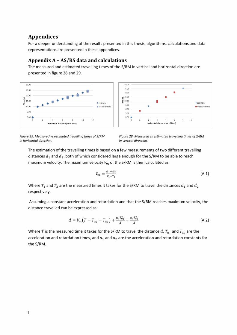
i

Appendices For a deeper understanding of the results presented in this thesis, algorithms, calculations and data

representations are presented in these appendices.

Appendix A – AS/RS data and calculations The measured and estimated travelling times of the S/RM in vertical and horizontal direction are

presented in figure 28 and 29.

The estimation of the travelling times is based on a few measurements of two different travelling

distances and both of which considered large enough for the S/RM to be able to reach

maximum velocity. The maximum velocity of the S/RM is then calculated as:

(A.1)

Where and are the measured times it takes for the S/RM to travel the distances and

respectively.

Assuming a constant acceleration and retardation and that the S/RM reaches maximum velocity, the

distance travelled can be expressed as:

(A.2)

Where is the measured time it takes for the S/RM to travel the distance , and

are the

acceleration and retardation times, and and are the acceleration and retardation constants for

the S/RM.

Figure 29. Measured vs estimated travelling times of S/RM in horizontal direction.

Figure 28. Measured vs estimated travelling times of S/RM in vertical direction.

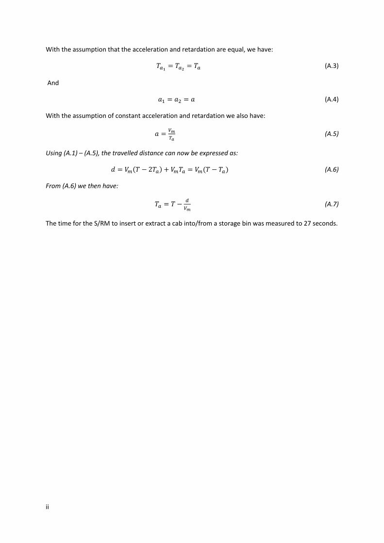
ii

With the assumption that the acceleration and retardation are equal, we have:

(A.3)

And

(A.4)

With the assumption of constant acceleration and retardation we also have:

(A.5)

Using (A.1) – (A.5), the travelled distance can now be expressed as:

(A.6)

From (A.6) we then have:

(A.7)

The time for the S/RM to insert or extract a cab into/from a storage bin was measured to 27 seconds.

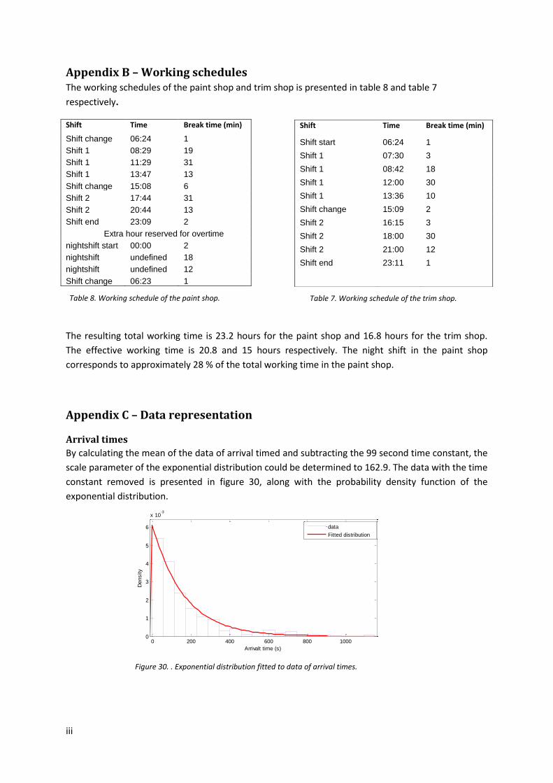
iii

0 200 400 600 800 10000

1

2

3

4

5

6

x 10-3

Arrivalt time (s)

Density

data

Fitted distribution

Appendix B – Working schedules The working schedules of the paint shop and trim shop is presented in table 8 and table 7

respectively.

Shift Time Break time (min)

Shift change 06:24 1

Shift 1 08:29 19

Shift 1 11:29 31

Shift 1 13:47 13

Shift change 15:08 6

Shift 2 17:44 31

Shift 2 20:44 13

Shift end 23:09 2

Extra hour reserved for overtime

nightshift start 00:00 2

nightshift undefined 18

nightshift undefined 12

Shift change 06:23 1

The resulting total working time is 23.2 hours for the paint shop and 16.8 hours for the trim shop.

The effective working time is 20.8 and 15 hours respectively. The night shift in the paint shop

corresponds to approximately 28 % of the total working time in the paint shop.

Appendix C – Data representation

Arrival times

By calculating the mean of the data of arrival timed and subtracting the 99 second time constant, the

scale parameter of the exponential distribution could be determined to 162.9. The data with the time

constant removed is presented in figure 30, along with the probability density function of the

exponential distribution.

Shift Time Break time (min)

Shift start 06:24 1

Shift 1 07:30 3

Shift 1 08:42 18

Shift 1 12:00 30

Shift 1 13:36 10

Shift change 15:09 2

Shift 2 16:15 3

Shift 2 18:00 30

Shift 2 21:00 12

Shift end 23:11 1

Figure 30. . Exponential distribution fitted to data of arrival times.

Table 8. Working schedule of the paint shop. Table 7. Working schedule of the trim shop.

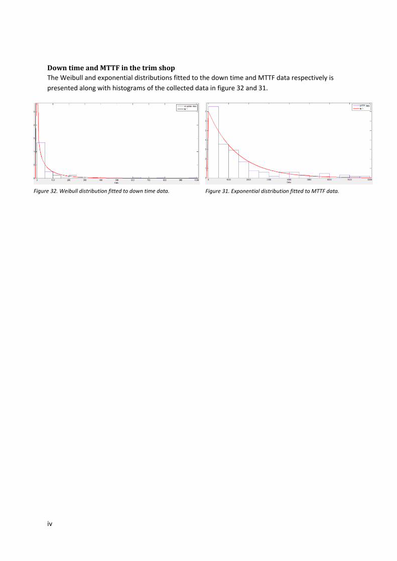
iv

Down time and MTTF in the trim shop

The Weibull and exponential distributions fitted to the down time and MTTF data respectively is

presented along with histograms of the collected data in figure 32 and 31.

Figure 32. Weibull distribution fitted to down time data. Figure 31. Exponential distribution fitted to MTTF data.

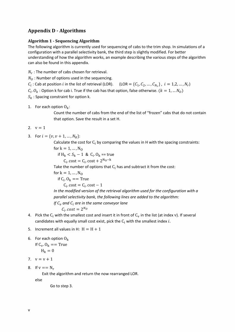
v

Appendix D - Algorithms

Algorithm 1 - Sequencing Algorithm

The following algorithm is currently used for sequencing of cabs to the trim shop. In simulations of a configuration with a parallel selectivity bank, the third step is slightly modified. For better understanding of how the algorithm works, an example describing the various steps of the algorithm can also be found in this appendix.

: The number of cabs chosen for retrieval.

: Number of options used in the sequencing.

: Cab at position in the list of retrieval (LOR). (LOR , )

: Option k for cab i. True if the cab has that option, false otherwise.

: Spacing constraint for option k.

1. For each option :

Count the number of cabs from the end of the list of “frozen” cabs that do not contain

that option. Save the result in a set H.

2.

3. For :

Calculate the cost for by comparing the values in H with the spacing constraints:

for

if & == true

Take the number of options that has and subtract it from the cost:

for

if

In the modified version of the retrieval algorithm used for the configuration with a

parallel selectivity bank, the following lines are added to the algorithm:

If and are in the same conveyor lane

4. Pick the with the smallest cost and insert it in front of in the list (at index ). If several

candidates with equally small cost exist, pick the with the smallest index .

5. Increment all values in H:

6. For each option

If

7. 8. If

Exit the algorithm and return the now rearranged LOR.

else

Go to step 3.

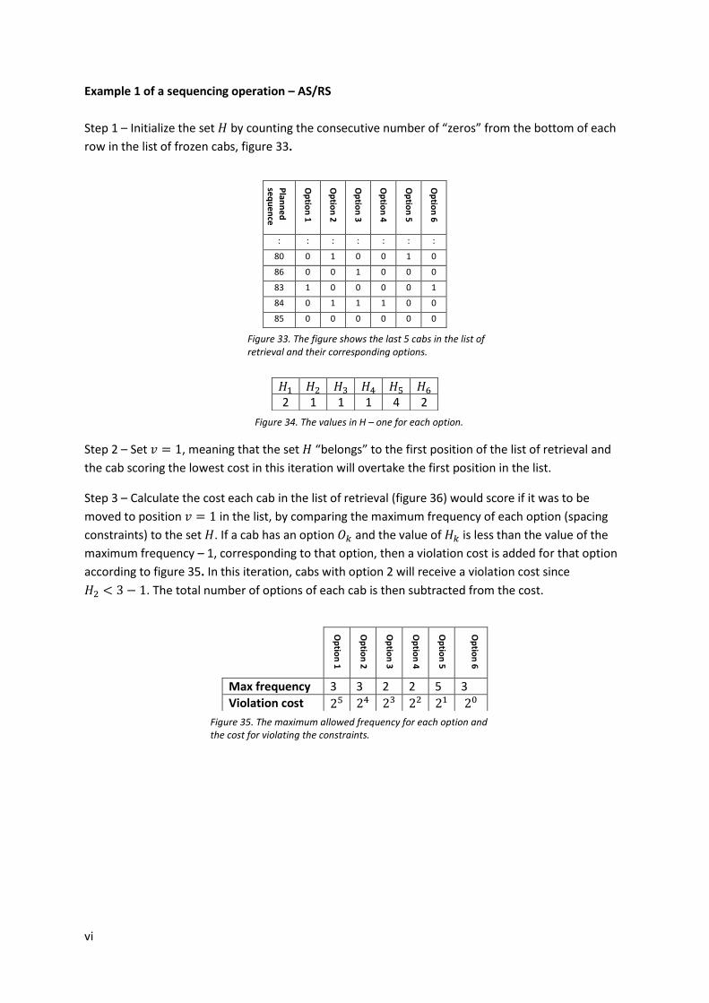
vi

Example 1 of a sequencing operation – AS/RS

Step 1 – Initialize the set by counting the consecutive number of “zeros” from the bottom of each

row in the list of frozen cabs, figure 33.

Step 2 – Set , meaning that the set “belongs” to the first position of the list of retrieval and

the cab scoring the lowest cost in this iteration will overtake the first position in the list.

Step 3 – Calculate the cost each cab in the list of retrieval (figure 36) would score if it was to be

moved to position in the list, by comparing the maximum frequency of each option (spacing

constraints) to the set . If a cab has an option and the value of is less than the value of the

maximum frequency – 1, corresponding to that option, then a violation cost is added for that option

according to figure 35. In this iteration, cabs with option 2 will receive a violation cost since

. The total number of options of each cab is then subtracted from the cost.

Plan

ne

d

seq

ue

nce

Op

tion

1

Op

tion

2

Op

tion

3

Op

tion

4

Op

tion

5

Op

tion

6

: : : : : : :

80 0 1 0 0 1 0

86 0 0 1 0 0 0

83 1 0 0 0 0 1

84 0 1 1 1 0 0

85 0 0 0 0 0 0

Figure 33. The figure shows the last 5 cabs in the list of retrieval and their corresponding options.

2 1 1 1 4 2

Figure 34. The values in H – one for each option.

Op

tion

1

Op

tion

2

Op

tion

3

Op

tion

4

Op

tion

5

Op

tion

6

Max frequency 3 3 2 2 5 3

Violation cost

Figure 35. The maximum allowed frequency for each option and the cost for violating the constraints.

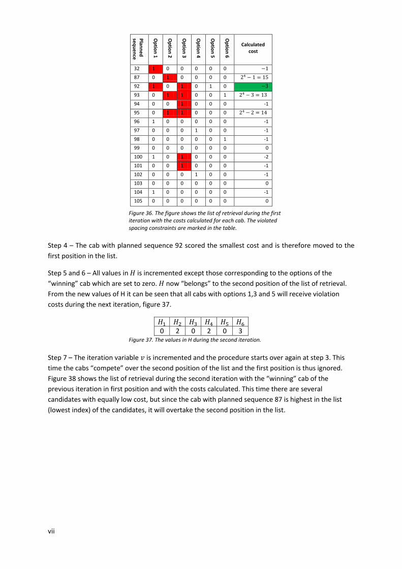
vii

Step 4 – The cab with planned sequence 92 scored the smallest cost and is therefore moved to the

first position in the list.

Step 5 and 6 – All values in is incremented except those corresponding to the options of the

“winning” cab which are set to zero. now “belongs” to the second position of the list of retrieval.

From the new values of H it can be seen that all cabs with options 1,3 and 5 will receive violation

costs during the next iteration, figure 37.

0 2 0 2 0 3

Step 7 – The iteration variable is incremented and the procedure starts over again at step 3. This

time the cabs “compete” over the second position of the list and the first position is thus ignored.

Figure 38 shows the list of retrieval during the second iteration with the “winning” cab of the

previous iteration in first position and with the costs calculated. This time there are several

candidates with equally low cost, but since the cab with planned sequence 87 is highest in the list

(lowest index) of the candidates, it will overtake the second position in the list.

Plan

ne

d

seq

ue

nce

Op

tion

1

Op

tion

2

Op

tion

3

Op

tion

4

Op

tion

5

Op

tion

6

Calculated

cost

32 1 0 0 0 0 0

87 0 1 0 0 0 0

92 1 0 1 0 1 0

93 0 1 1 0 0 1

94 0 0 1 0 0 0 -1

95 0 1 1 0 0 0

96 1 0 0 0 0 0 -1

97 0 0 0 1 0 0 -1

98 0 0 0 0 0 1 -1

99 0 0 0 0 0 0 0

100 1 0 1 0 0 0 -2

101 0 0 1 0 0 0 -1

102 0 0 0 1 0 0 -1

103 0 0 0 0 0 0 0

104 1 0 0 0 0 0 -1

105 0 0 0 0 0 0 0

Figure 36. The figure shows the list of retrieval during the first iteration with the costs calculated for each cab. The violated spacing constraints are marked in the table.

Figure 37. The values in H during the second iteration.

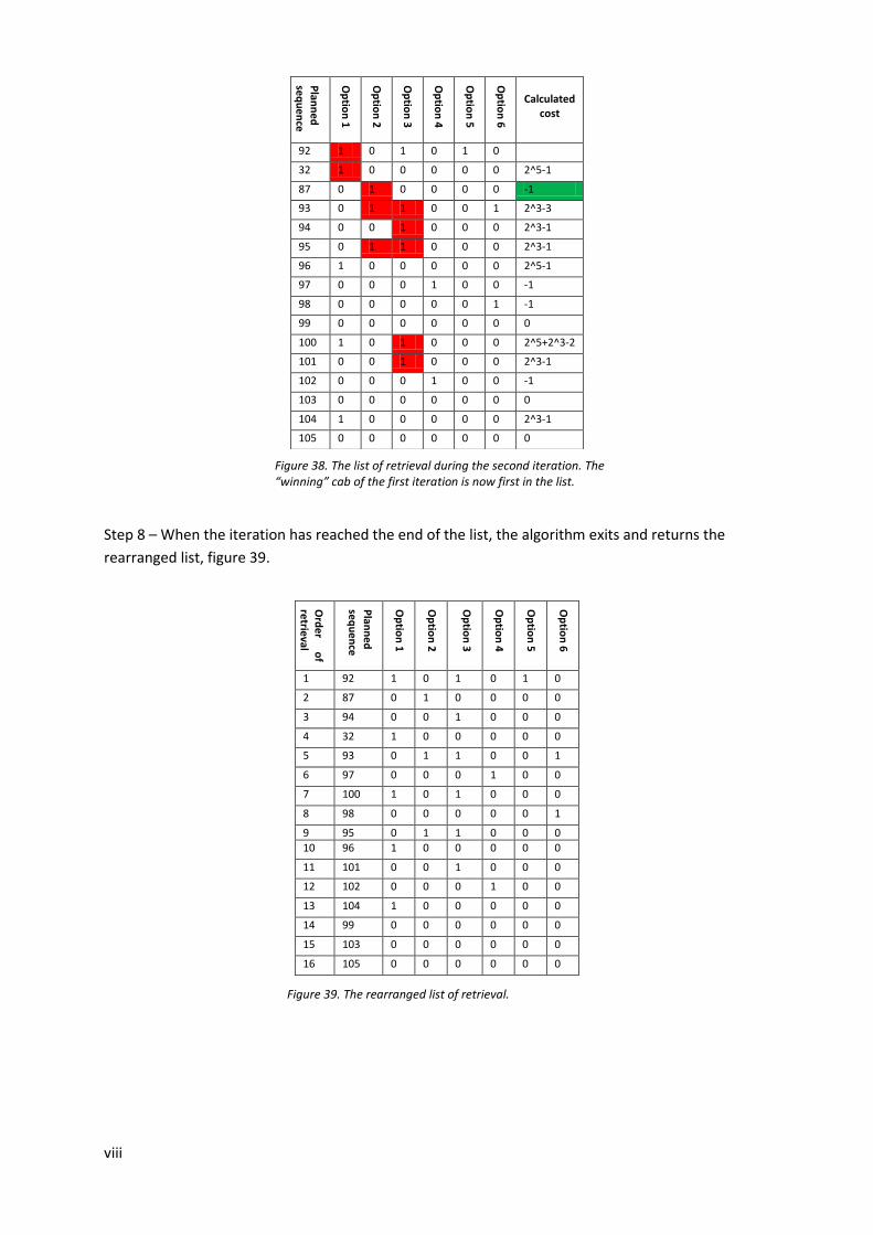
viii

Step 8 – When the iteration has reached the end of the list, the algorithm exits and returns the

rearranged list, figure 39.

Plan

ne

d

seq

ue

nce

Op

tion

1

Op

tion

2

Op

tion

3

Op

tion

4

Op

tion

5

Op

tion

6

Calculated

cost

92 1 0 1 0 1 0

32 1 0 0 0 0 0 2^5-1

87 0 1 0 0 0 0 -1

93 0 1 1 0 0 1 2^3-3

94 0 0 1 0 0 0 2^3-1

95 0 1 1 0 0 0 2^3-1

96 1 0 0 0 0 0 2^5-1

97 0 0 0 1 0 0 -1

98 0 0 0 0 0 1 -1

99 0 0 0 0 0 0 0

100 1 0 1 0 0 0 2^5+2^3-2

101 0 0 1 0 0 0 2^3-1

102 0 0 0 1 0 0 -1

103 0 0 0 0 0 0 0

104 1 0 0 0 0 0 2^3-1

105 0 0 0 0 0 0 0

Figure 38. The list of retrieval during the second iteration. The “winning” cab of the first iteration is now first in the list.

Ord

er

of

retrie

val

Plan

ne

d

seq

ue

nce

Op

tion

1

Op

tion

2

Op

tion

3

Op

tion

4

Op

tion

5

Op

tion

6

1 92 1 0 1 0 1 0

2 87 0 1 0 0 0 0

3 94 0 0 1 0 0 0

4 32 1 0 0 0 0 0

5 93 0 1 1 0 0 1

6 97 0 0 0 1 0 0

7 100 1 0 1 0 0 0

8 98 0 0 0 0 0 1

9 95 0 1 1 0 0 0

10 96 1 0 0 0 0 0

11 101 0 0 1 0 0 0

12 102 0 0 0 1 0 0

13 104 1 0 0 0 0 0

14 99 0 0 0 0 0 0

15 103 0 0 0 0 0 0

16 105 0 0 0 0 0 0

Figure 39. The rearranged list of retrieval.

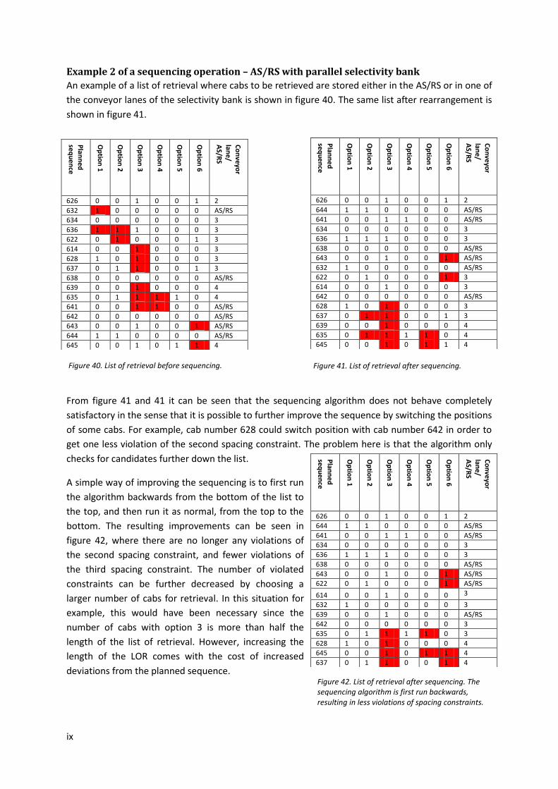
ix

Example 2 of a sequencing operation – AS/RS with parallel selectivity bank

An example of a list of retrieval where cabs to be retrieved are stored either in the AS/RS or in one of

the conveyor lanes of the selectivity bank is shown in figure 40. The same list after rearrangement is

shown in figure 41.

From figure 41 and 41 it can be seen that the sequencing algorithm does not behave completely

satisfactory in the sense that it is possible to further improve the sequence by switching the positions

of some cabs. For example, cab number 628 could switch position with cab number 642 in order to

get one less violation of the second spacing constraint. The problem here is that the algorithm only

checks for candidates further down the list.

A simple way of improving the sequencing is to first run

the algorithm backwards from the bottom of the list to

the top, and then run it as normal, from the top to the

bottom. The resulting improvements can be seen in

figure 42, where there are no longer any violations of

the second spacing constraint, and fewer violations of

the third spacing constraint. The number of violated

constraints can be further decreased by choosing a

larger number of cabs for retrieval. In this situation for

example, this would have been necessary since the

number of cabs with option 3 is more than half the

length of the list of retrieval. However, increasing the

length of the LOR comes with the cost of increased

deviations from the planned sequence.

Plan

ne

d

seq

ue

nce

Op

tion

1

Op

tion

2

Op

tion

3

Op

tion

4

Op

tion

5

Op

tion

6

Co

nve

yor

lane

/ A

S/RS

626 0 0 1 0 0 1 2

632 1 0 0 0 0 0 AS/RS

634 0 0 0 0 0 0 3

636 1 1 1 0 0 0 3

622 0 1 0 0 0 1 3

614 0 0 1 0 0 0 3

628 1 0 1 0 0 0 3

637 0 1 1 0 0 1 3

638 0 0 0 0 0 0 AS/RS

639 0 0 1 0 0 0 4

635 0 1 1 1 1 0 4

641 0 0 1 1 0 0 AS/RS

642 0 0 0 0 0 0 AS/RS

643 0 0 1 0 0 1 AS/RS

644 1 1 0 0 0 0 AS/RS

645 0 0 1 0 1 1 4

Plan

ne

d

seq

ue

nce

Op

tion

1

Op

tion

2

Op

tion

3

Op

tion

4

Op

tion

5

Op

tion

6

Co

nve

yor

lane

/ A

S/RS

626 0 0 1 0 0 1 2

644 1 1 0 0 0 0 AS/RS

641 0 0 1 1 0 0 AS/RS

634 0 0 0 0 0 0 3

636 1 1 1 0 0 0 3

638 0 0 0 0 0 0 AS/RS

643 0 0 1 0 0 1 AS/RS

632 1 0 0 0 0 0 AS/RS

622 0 1 0 0 0 1 3

614 0 0 1 0 0 0 3

642 0 0 0 0 0 0 AS/RS

628 1 0 1 0 0 0 3

637 0 1 1 0 0 1 3

639 0 0 1 0 0 0 4

635 0 1 1 1 1 0 4

645 0 0 1 0 1 1 4

Plan

ne

d

seq

ue

nce

Op

tion

1

Op

tion

2

Op

tion

3

Op

tion

4

Op

tion

5

Op

tion

6

Co

nve

yor

lane

/ A

S/RS

626 0 0 1 0 0 1 2

644 1 1 0 0 0 0 AS/RS

641 0 0 1 1 0 0 AS/RS

634 0 0 0 0 0 0 3

636 1 1 1 0 0 0 3

638 0 0 0 0 0 0 AS/RS

643 0 0 1 0 0 1 AS/RS

622 0 1 0 0 0 1 AS/RS

614 0 0 1 0 0 0 3

632 1 0 0 0 0 0 3

639 0 0 1 0 0 0 AS/RS

642 0 0 0 0 0 0 3

635 0 1 1 1 1 0 3

628 1 0 1 0 0 0 4

645 0 0 1 0 1 1 4

637 0 1 1 0 0 1 4

Figure 40. List of retrieval before sequencing. Figure 41. List of retrieval after sequencing.

Figure 42. List of retrieval after sequencing. The sequencing algorithm is first run backwards, resulting in less violations of spacing constraints.

x

Algorithm 2 - Algorithm for choosing conveyor lane

The following algorithm is used in simulation for selecting a conveyor lane for storing an arriving cab.

– Difference between the scheduled sequence position of the cab to be stored and the rearmost

cab in lane :

– The cab to be stored is scheduled for assembly work cycles earlier than the rearmost

cab.

– The cab to be stored is scheduled for assembly work cycles later than the rearmost cab.

– User defined parameter

– Maximum capacity of lane .

– Number of cabs in lane .

– Number of lanes in the selectivity bank.

1. If there is an empty lane

Cost = 0

Choose the empty lane for storing the cab and exit the algorithm.

2. .

3. If

Else

4. If AND

Cost = tempcost

k = i

5. If

Choose lane k for storing the cab and exit the algorithm. The Cost variable is also returned.

Else

Go to step 3.

Several values of the parameter were tested in simulations. It was then set to 0.5 which resulted in

a good balance between deviations of the planned sequence to the trim shop and flow of cabs

through the selectivity bank.

xi

Control Method The control method described here is used in simulations to determine if a cab should be stored in

the AS/RS or the selectivity bank. Every time a cab is stored or retrieved from the buffer, the

parameter is updated using (D.5) – (D.9). When a cab arrives to the buffer, the cost calculated in

algorithm 2 is compared to . If the calculated cost is smaller than , the cab is stored in the chosen

lane in the selectivity bank. Otherwise it is stored in the AS/RS.

In the PBS, there are two main events occurring which are triggered from outside the PBS and

therefore considered uncontrollable in this thesis. These are when cabs enter the PBS and when cabs

are retrieved from the PBS. This control method is only used when a cab enters the PBS and

therefore this event is used as the time instant, denoted k.

The number of cabs stored in the selectivity bank during a time of can be expressed as:

(D.1)

The number of cabs retrieved from the selectivity bank during a time of can be expressed as:

(D.2)

The change in the number of cabs in the selectivity bank can then be expressed as

(D.3)

Using a proportional control approach, we can based on the desired buffer level , express a desired

change of the buffer level of the selectivity bank as:

(D.4)

Where is a gain parameter.

From (D.3) and (D.4) we get the desired input to the selectivity bank .

(D.5)

The control variable is then updated by comparing the desired input with the desired

input and using an appropriate value on the step size :

(D.6)

In order to avoid negative or too small values as well as too large values of beta, limits are also

defined for according to:

(D.7)

xii

By using the control method described above during the day and evening shifts, the number of cabs

in the selectivity bank during the start of the night shift should be approximately equal to .

During the night shift it is desirable that the selectivity bank is filled up at an even pace so that it gets

full at approximately the same time as the night shift ends.

The desired input to the selectivity bank during the night shift thus becomes:

(D.8)

Where is the estimated number of cabs to be produced during the night shift and is the

total capacity of the selectivity bank.

In order to avoid large queue build-up, the reference level is increased proportionally to the number

of cabs currently in queue according to:

(D.9)

Where is the number of cabs waiting in queue to the PBS and is a gain parameter.

Parameters used in simulation:

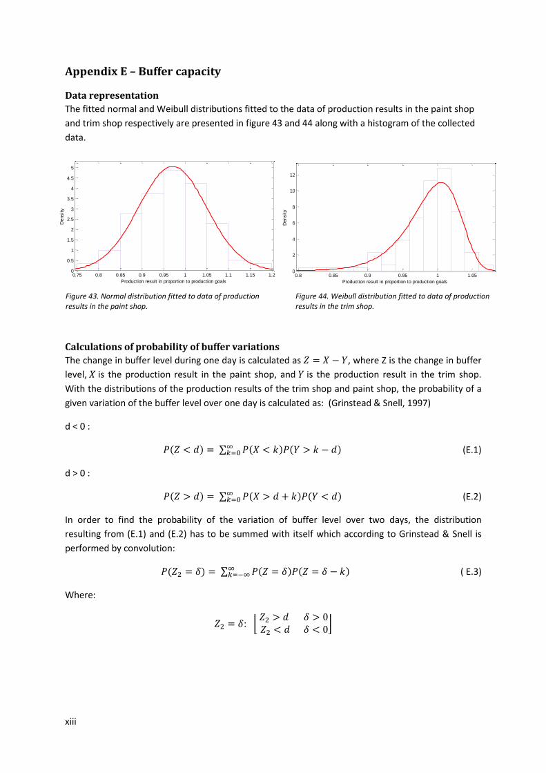
xiii

0.8 0.85 0.9 0.95 1 1.050

2

4

6

8

10

12

Density

Production result in proportion to production goals

Ptrim data

fit 1

0.75 0.8 0.85 0.9 0.95 1 1.05 1.1 1.15 1.20

0.5

1

1.5

2

2.5

3

3.5

4

4.5

5

Density

Production result in proportion to production goals

Ppaint data

fit 1

Appendix E – Buffer capacity

Data representation

The fitted normal and Weibull distributions fitted to the data of production results in the paint shop

and trim shop respectively are presented in figure 43 and 44 along with a histogram of the collected

data.

Calculations of probability of buffer variations

The change in buffer level during one day is calculated as , where Z is the change in buffer

level, is the production result in the paint shop, and is the production result in the trim shop.

With the distributions of the production results of the trim shop and paint shop, the probability of a

given variation of the buffer level over one day is calculated as: (Grinstead & Snell, 1997)

d < 0 :

(E.1)

d > 0 :

(E.2)

In order to find the probability of the variation of buffer level over two days, the distribution

resulting from (E.1) and (E.2) has to be summed with itself which according to Grinstead & Snell is

performed by convolution:

( E.3)

Where:

:

Figure 43. Normal distribution fitted to data of production results in the paint shop.

Figure 44. Weibull distribution fitted to data of production results in the trim shop.

xiv

The probability that the upper or lower buffer limit is exceeded by number of cabs is given by:

d < 0:

(E.4)

d > 0:

(E.5)

Where is the number of cabs in the normal interval.

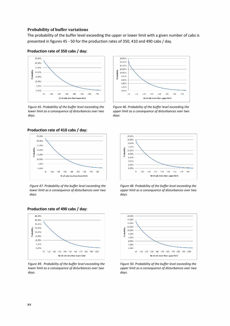
xv

Probability of buffer variations

The probability of the buffer level exceeding the upper or lower limit with a given number of cabs is

presented in figures 45 - 50 for the production rates of 350, 410 and 490 cabs / day.

Production rate of 350 cabs / day:

Production rate of 410 cabs / day:

Production rate of 490 cabs / day:

Figure 45. Probability of the buffer level exceeding the lower limit as a consequence of disturbances over two days.

Figure 46. Probability of the buffer level exceeding the upper limit as a consequence of disturbances over two days.

Figure 47. Probability of the buffer level exceeding the lower limit as a consequence of disturbances over two days.

Figure 48. Probability of the buffer level exceeding the upper limit as a consequence of disturbances over two days.

Figure 49. Probability of the buffer level exceeding the lower limit as a consequence of disturbances over two days.

Figure 50. Probability of the buffer level exceeding the upper limit as a consequence of disturbances over two days.