Analysis of a new dimension-wise splitting iteration …gander/Preprints/DSSR.pdfAnalysis of a new dimension-wise splitting iteration with selective relaxation 3 A different idea is

BIT manuscript No.(will be inserted by the editor)

Analysis of a new dimension-wise splitting iteration withselective relaxation for saddle point problems

Martin J. Gander · Qiang Niu · Yingxiang Xu

Received: date / Accepted: date

Abstract We propose a new Dimension-wise Splitting with Selective Relaxation(DSSR) method for saddle point systems arising from the discretization of the incom-pressible Navier-Stokes equations. Using Fourier analysis, we determine the optimalchoice of the relaxation parameter that leads to the best performance of the iterativemethod for the Stokes and the steady Oseen equations. We also explore numericallythe influence of boundary conditions on the optimal choice of the parameter, the useof inner and outer iterations, and the performance for a lid driven cavity flow.

Keywords splitting iterations · optimized relaxation parameter · Stokes · Oseen

Mathematics Subject Classification (2000) 65F10 · 65N22

1 Introduction

We consider the steady incompressible Navier-Stokes equations

−ν∆u+u ·∇u+∇p = f, in Ω ,∇ ·u = 0, in Ω ,

u = g, on ∂Ω ,(1.1)

M.J. GanderSection de Mathematiques, Universite de Geneve, 2-4 rue du Lievre, CP 64, CH-1211, Geneva, Switzer-land. E-mail: [email protected]

Q. NiuDepartment of Mathematical Sciences, Xi’an Jiaotong-Liverpool University, Suzhou 215123, China. E-mail: [email protected], partially supported by NSFC-11301420

Y. XuCorresponding author. School of Mathematics and Statistics, Northeast Normal University, Changchun130024, China. E-mail: [email protected], partially supported by NSFC-11201061, 11471047,11271065, CPSF-2012M520657 and the Science and Technology Development Planning of Jilin Province20140520058JH

2 Martin J. Gander et al.

where u is the velocity field, p is the pressure, ν is the given kinematic viscositydetermined by the fluid (ν is inversely proportional to the Reynolds number), and thedomain Ω is an open bounded domain in R2 (or R3).

Equation (1.1) is nonlinear because of the transport term u ·∇u. A popular strat-egy for dealing with this nonlinearity is to use a relaxation for the nonlinear term: find(uk, pk) with an initial guess on the velocity field u0 satisfying ∇u0 = 0 by solving

−ν∆uk +uk−1 ·∇uk +∇pk = f, in Ω ,∇ ·uk = 0, in Ω ,

uk = g, on ∂Ω .(1.2)

Discretizing equation (1.2) using a finite element or finite difference method leads toa so-called saddle point problem

Hz = b, (1.3)

where in 2D

H =

A1 0 BT1

0 A2 BT2

−B1 −B2 0

and z =(

up

),

and H is a sparse matrix in Rn×n, b ∈ Rn is the right hand side that depends on thegiven data f and g, and we are solving for the unknown z ∈ Rn.

Problem (1.3) is a typical saddle point problem, which arises also in many otherapplications throughout computational science and engineering, and the iterative so-lution of such problems has been the focus of intense research efforts, see for examplethe review [10]. In addition to the block preconditioners based on approximate com-mutators [15,18] and least squares [16], one of the successful iterative methods forsolving saddle point problems is the Hermitian and skew-Hermitian splitting (HSS)method invented by Bai, Golub and Ng [5], where the system matrix H is split intoits Hermitian and non-Hermitian parts, and then an ADI like iterative scheme is used,solving only Hermitian and skew-Hermitian problems, and a relaxation parameter α

is introduced to obtain rapid convergence. Like all stationary iterative methods, HSSalso defines naturally a preconditioner that can be used to accelerate a Krylov method.

A substantial development followed this seminal work, with an important focuson how one should choose the relaxation parameter α to get fast convergence for agiven class of problems. For example, Bai, Golub and Li [3] optimized the spectralradius of the iteration matrix and obtained an eigenvalue-based optimized relaxationparameter α∗. In [2], the authors proposed a new variant of HSS called acceleratedHermitian and skew-Hermitian splitting (AHSS), which improved the HSS methodby introducing an extra relaxation parameter in order to shift the non-Hermitian partdifferently. These two parameters were then optimized for performance, and the op-timal choice was shown to be related to the singular values of a certain matrix arisingin the iteration. A more concrete estimate was given by Bai [1] with an analysis atthe continuous level, by optimizing an approximation of the spectral radius of the it-eration matrix, which leads to quasi-optimal parameters. The main difficulty in theseapproaches based on the matrix H itself is to obtain the estimates on the quantities onwhich the optimized relaxation parameter depends on.

Analysis of a new dimension-wise splitting iteration with selective relaxation 3

A different idea is to relate the iteration back to the underlying physical operator,from which the matrix H was obtained by discretization. This was proposed by Benzi,Gander and Golub [9], where the HSS iteration was related back to the underlyingLaplace operator written in mixed form. This can be achieved using Fourier analysis,and can lead to accurate predictions for the optimized relaxation parameter. Thisanalysis also revealed a new feature of HSS, when used as a preconditioner for aKrylov method: instead of minimizing the spectral radius, a different choice of therelaxation parameter leads to two very small and tight clusters in the spectrum of theHSS preconditioned operator, which then leads to convergence in two iterations whensolving the preconditioned system using a Krylov method. Fourier analysis can thusbe very helpful for understanding the performance of iterative methods, see also [19,21,20,7,22,23,8].

More recently, new stationary iterative methods were proposed for saddle pointproblems. In particular, Benzi and Guo [11] proposed the dimensional splitting pre-conditioner for saddle point problems arising from the discretization of the Navier-Stokes equation, where there is also a relaxation parameter, but the optimization prob-lem was not addressed. Benzi et al. [12] proposed a further variant called RelaxedDimensional Factorization (RDF) preconditioner, directly to be used with a Krylovmethod. They did consider the optimization of the relaxation parameter, but withoutstudying the preconditioner as a stationary iterative method.

In this paper, we present and analyze a new method based on a Dimension-wiseSplitting with Selective Relaxation (DSSR) that can be used both as an iterative solverand a preconditioner for a Krylov method, see also [14]. We prove first that the DSSRiteration converges unconditionally for any relaxation parameter α > 0 when themethod is applied to the 2D Stokes problem. We also show how Fourier analysiscan be used to optimize the relaxation parameter of the method, both to minimizethe spectral radius and to form tight clusters in the spectrum of the preconditionedoperator. We find that the optimal choice for the relaxation parameter α is inverselyproportional to the viscosity ν , and with this choice the convergence rates are robustin ν . We then extend our results to the 3D Stokes and Oseen equations. Using numer-ical experiments, we illustrate that the theoretically optimized parameters are stillasymptotically optimal and robust also in the presence of Dirichlet boundary condi-tions, where the Fourier analysis is not valid any more. We also show numericallythat DSSR is competitive with RDF, which was recently shown to outperform manyother preconditioners, and test the use of inexact inner solves, which leads to innerand outer iterations.

2 Dimension-wise splitting with selective relaxation (DSSR)

The dimension-wise splitting with selective relaxation is based on the decompositionof the system matrix in (1.3) into H = H1 +H2 [11,12], where

H1 =

A1 0 BT1

0 0 0−B1 0 0

and H2 =

0 0 00 A2 BT

20 −B2 0

. (2.1)


To add a relaxation parameter θ , we define the diagonal matrices

E1 := diag(0, I,θ I) and E2 := diag(I,0,(1−θ)I)

with 0 < θ < 1, where the block sizes of the zero matrices 0 and the identity matricesI correspond to the block sizes of the submatrices in (2.1).

We can thus define two splittings of the system matrix H with further relaxationparameter α > 0,

H = (αE1 +H1)− (αE1−H2) and H = (αE2 +H2)− (αE2−H1).

Note here that both

αE1 +H1 =

A1 0 BT1

0 αI 0−B1 0 αθ I

and αE2 +H2 =

αI 0 00 A2 BT

20 −B2 α(1−θ)I

are nonsingular matrices, provided that the boundary conditions imposed on the ve-locity components lead to invertible discrete Laplace operators. The DSSR algorithmconsists of the alternating solution between these two splittings: given an initial guessz0 = (u0, p0), the iteration computes a sequence of approximations zk defined by

(αE1 +H1)zk+ 12 = (αE1−H2)zk +b,

(αE2 +H2)zk+1 = (αE2−H1)zk+ 12 +b.

(2.2)

The DSSR algorithm can be rewritten in fixed point form by eliminating the interme-diate vector zk+ 1

2 , and we obtain

zk+1 = Mα zk +Nα b, (2.3)

whereMα = (αE2 +H2)

−1(αE2−H1)(αE1 +H1)−1(αE1−H2)

andNα = (αE2 +H2)

−1[(αE2−H1)(αE1 +H1)−1 + I].

Theorem 2.1 The fixed point z∗ of (2.3) is solution to (1.3).

Proof It is easy to verify by a direct calculation that

αH = α(H1 +H2)= (αE1 +H1)(αE2 +H2)− (αE2−H1)(αE1−H2)= (αE1 +H1)(αE2 +H2)− (αE2−H1)(αE1 +H1)(αE1 +H1)

−1(αE1−H2)= (αE1 +H1)(αE2 +H2)− (αE1 +H1)(αE2−H1)(αE1 +H1)

−1(αE1−H2).

Multiplying this equation by (αE2 +H2)−1(αE1 +H1)

−1 from the left on both sidesyields

α(αE2 +H2)−1(αE1 +H1)

−1H = I−Mα .

We can now multiply both sides from the right by the fixed point vector z∗ of theiteration (2.3), and obtain

α(αE2+H2)−1(αE1+H1)

−1Hz∗ = (αE2+H2)−1((αE2−H1)(αE1+H1)

−1+ I)b.


Now since the right hand side of this equation satisfies

(αE2 +H2)−1((αE2−H1)(αE1 +H1)

−1 + I)b= (αE2 +H2)

−1((αE2−H1)(αE1 +H1)−1 +(αE1 +H1)(αE1 +H1)

−1)b= (αE2 +H2)

−1(αE1 +αE2)(αE1 +H1)−1b

= α(αE2 +H2)−1(αE1 +H1)

−1b,

we obtain the desired result Hz∗ = b, which concludes the proof.

The DSSR iteration (2.2) can also be rewritten in correction form, namely

zk+1 = zk +P−1α rk, rk = b−Hzk,

where Pα := 1α(αE1 +H1)(αE2 +H2). Note that Mα = I−P−1

α H. In addition, weknow that using a Krylov subspace method to accelerate the convergence of the DSSRiteration is equivalent to the application of the Krylov subspace method to the precon-ditioned system P−1

α Hz = P−1α b in the case of left preconditioning, or to HP−1

α y = b,y = Pα z for right preconditioning.

3 Convergence analysis of DSSR at the continuous level

It is well known that the iterative scheme (2.2) converges for any initial guess z0,if the spectral radius of Mα is strictly less than one, ρ(Mα) < 1. In order to obtainfast convergence, the parameters θ and α should be chosen to make the spectralradius small. This is in general a difficult problem at the linear algebra level. One canhowever optimize the parameters in the method using the fact that the matrices arediscretizations of underlying differential operators, see e.g. [9].

3.1 Analysis of DSSR for the Stokes equation in 2D

We start by considering the Stokes equation in the unbounded domain R2,

−ν∆u+∂x p = f1,−ν∆v+∂y p = f2,

∂xu+∂yv = 0.(3.1)

From the analysis in Appendix A we see that for the Stokes problem, i.e. without theadvection term, the best parameter choice for θ is θ = 1

2 , and we thus only have oneparameter left to optimize. Writing the Stokes equation (3.1) in matrix form yields−ν∆ 0 ∂x

0 −ν∆ ∂y∂x ∂y 0

uvp

=

f1f20

.

Following the approach in [9], we take a Fourier transform in both the x and y direc-tions and obtain for each Fourier mode (k1,k2) the linear systemν(k2

1 + k22) 0 ik1

0 ν(k21 + k2

2) ik2ik1 ik2 0

uvp

=

f1f20

.


This has the great advantage that we can now study the performance of the DSSRalgorithm for each Fourier mode separately. Note however that this neglects bound-ary conditions in the analysis, which we will see play a certain role as well for theiteration.

The Fourier transformed linear operator H corresponding to the Stokes equation(3.1) is thus given by

H =

ν(k21 + k2

2) 0 ik10 ν(k2

1 + k22) ik2

ik1 ik2 0

,

and we can also write the dimension-wise splitting operators H1 and H2 after theFourier transform,

H1 =

ν(k21 + k2

2) 0 ik10 0 0

ik1 0 0

and H2 =

0 0 00 ν(k2

1 + k22) ik2

0 ik2 0

.

Thus, the Fourier transformed iteration matrix of the DSSR algorithm is given by

Mα = (αE2 + H2)−1(αE2− H1)(αE1 + H1)

−1(αE1− H2),

with E1 = diag(0,1,1/2) and E2 = diag(1,0,1/2). The eigenvalues of the Fouriertransformed iteration matrix Mα can now simply be calculated, and we get

λ1,2(k1,k2) = 0, λ3(k1,k2) =αν(k2

1 + k22)−2k2

1

αν(k21 + k2

2)+2k21· αν(k2

1 + k22)−2k2

2

αν(k21 + k2

2)+2k22.

Thus the spectral radius of Mα is given by

ρ(k1,k2,ν ,α) = |λ3(k1,k2)|.

Note that ρ depends only on k21 and k2

2, and thus it is sufficient to analyze the algorithmfor positive Fourier frequencies k1,k2 > 0. A direct calculation shows that

liminfk1,k2→0

λ3(k1,k2) =αν−2αν +2

= liminfk1,k2→∞

λ3(k1,k2).

Together with the fact that ρ(k1,k2,ν ,α) < 1 for any fixed k1,k2, we thus arrive atthe following convergence theorem.

Theorem 3.1 The DSSR iteration (2.2) applied to a consistently discretized versionof the Stokes problem (3.1) on an unbounded domain converges for any α > 0, pro-vided the mesh size is small enough.

To optimize the performance of the DSSR iteration, we need to choose the re-laxation parameter α to minimize the maximum of the spectral radius ρ(k1,k2,ν ,α)over all Fourier frequencies (k1,k2), which means that we have to solve the min-maxproblem

minα>0

maxk1,k2>0

ρ(k1,k2,ν ,α). (3.2)


Theorem 3.2 The parameter value α∗ =√

3ν

solves the min-max problem (3.2), andthe corresponding optimized spectral radius of Mα satisfies

maxk1,k2>0

ρ(k1,k2,ν ,α∗) =

2−√

32+√

3.

Proof A direct calculation shows that

∂λ3

∂k1=− 32k1k2

2αν(k41− k4

2)

(αν(k21 + k2

2)+2k22)

2(αν(k21 + k2

2)+2k21)

2 , (3.3)

which is positive for 0 < k1 < k2, and negative for k1 > k2 > 0. Similarly we obtainthat

∂λ3

∂k2=

32k2k21αν(k4

1− k42)

(αν(k21 + k2

2)+2k22)

2(αν(k21 + k2

2)+2k21)

2 , (3.4)

which is positive for k1 > k2 > 0, and negative for 0 < k1 < k2. We therefore obtainthat at the zero of the two functions (3.3) and (3.4), k1 = k2, the function λ3 attainsits maximum. Inserting k1 = k2 shows that the maximum value of λ3 is given byλ3(k1,k1) =

(αν−1αν+1

)2, independently of k1.

Since ∂λ3∂k1

> 0 for k1 < k2, λ3 is monotonically increasing in k1 for k1 ∈ (0,k2),

and since ∂λ3∂k2

> 0 for k2 < k1, λ3 is monotonically increasing in k2 for k2 ∈ (0,k1).Thus, limk1→0 λ3 =

αν−2αν+2 = limk2→0 λ3 is a potential minimum of λ3 for k1,k2 > 0.

Next, since ∂λ3∂k1

< 0 for k1 > k2, λ3 is monotonically decreasing in k1 for k1 > k2,

and since ∂λ3∂k2

< 0 for k2 > k1, λ3 is monotonically decreasing in k2 for k2 > k1. Thuslimk1→∞ λ3 =

αν−2αν+2 = limk2→∞ λ3 is another potential minimum of λ3 for k1,k2 > 0.

We therefore see that ρ(k1,k2,ν ,α) has two potential extrema:∣∣αν−2

αν+2

∣∣ when k1

or k2 tend to 0 or ∞, and(

αν−1αν+1

)2 for k1 = k2.We show below that solving the equi-oscillation equation gives the best choice,(

αν−1αν +1

)2

=

∣∣∣∣αν−2αν +2

∣∣∣∣ =⇒ α∗ =

√3

ν, (3.5)

with the corresponding spectral radius maxk1,k2>0 ρ(k1,k2,ν ,α) = 2−√

32+√

3≈ 0.0718.

To prove that α∗ given in (3.5) indeed solves the min-max problem (3.2), note that(αν−1αν+1

)2 is monotonically increasing in α for α ∈ ( 1ν,∞), and thus α > α∗ would

lead to a larger spectral radius for Mα . Similarly, αν−2αν+2 is monotonically decreasing

in α for 2/ν > α > 0, and thus α < α∗ would lead to a larger spectral radius for Mα ,which concludes the proof.

If DSSR is used as a preconditioner for a Krylov subspace method, one can usethe same relaxation parameter α∗ from (3.5) that was optimized for the stationaryiteration, since minimizing the spectral radius corresponds to clustering the eigenval-ues of the preconditioned operator around 1. However for DSSR there exists also adifferent option: one can form two tight separate clusters with an appropriate choiceof the optimization parameter α , as we show next.


Lemma 3.1 The eigenvalues λ3(k1,k2) for k1,k2 > 0 are real and contained in theinterval T =

(αν−2αν+2 ,(

αν−1αν+1 )

2].

Proof This result follows directly from the proof of Theorem 3.2.

Note that the length of the interval T , which is given by 4(αν+1)2(αν+2) > 0 tends to

zero as αν tends to infinity.

Lemma 3.2 There exists a polynomial p2(x) of order 2 which satisfies p2(0) = 1,p2(1) = 0 and on the shifted interval Ts =

(1− αν−2

αν+2 ,1− (αν−1αν+1 )

2]

maxx∈Ts|p2(x)| ≤ q2(α,ν),

where

q2(α,ν) =(αν)3−4(αν)2 +5(αν)−2

2(αν)5 +4(αν)4−5(αν)3−12(αν)2−3(αν)−2

=1

2(αν)2 +O(1

(αν)3 ). (3.6)

Proof We assume that the polynomial p2(x) has the form p2(x) = 1+bx+cx2, sinceit satisfies p2(0) = 1. Using the condition p2(1) = 0 we get

1+b+ c = 0. (3.7)

Since this polynomial is convex, it will attain on the interval Ts its maximum on theleft end point 1− (αν−1

αν+1 )2 and its minimum on the right end point 1− αν−2

αν+2 . Thussetting the absolute values of p2(x) at 1− (αν−1

αν+1 )2 and 1− αν−2

αν+2 equal, together with(3.7), we can derive the values of b and c, and thus the polynomial p2(x). We thereforeobtain the maximum value of p2(x) on the interval to be

p2

(1−(

αν−1αν +1

)2)

=(αν)3−4(αν)2 +5(αν)−2

2(αν)5 +4(αν)4−5(αν)3−12(αν)2−3(αν)−2.

Expanding in αν for αν large we find (3.6), which concludes the proof.

Since the DSSR preconditioned Stokes system is diagonalizable with an orthogonalbasis, we get a convergence theorem for GMRES with p2(x) as residual polynomial:

Theorem 3.3 GMRES applied to the preconditioned fixed point system (I−Mα)z =Nα b from (2.3) converges in the case of a fine enough discretized Stokes system (3.1)on an unbounded domain in at most two iteration steps to a given small tolerance τ

if the optimized parameter α∗ satisfies q2(α∗) = τ , which implies asymptotically that

α∗ ≈ 1ν

√1

2τ.

One can also estimate the decay of a higher order residual polynomial, for exampleof degree three:


Lemma 3.3 There exists a polynomial p3(x) of order 3 which satisfies p3(0) = 1,p3(1) = 0 and on the shifted interval Ts

maxx∈Ts|p3(x)| ≤ q3(α,ν),

where q3(α,ν) is explicitly known and has the asymptotic expansion q3(α,ν) =1

8(αν)4 +O(

1(αν)5

).

Proof Similar to the proof of Lemma 3.2 we assume that the polynomial p3(x) hasthe form p3(x) = 1+bx+ cx2 +dx3. Since we require p3(1) = 0 we get

1+b+ c+d = 0. (3.8)

Denote by x1 = 1− (αν−1αν+1 )

2 and x2 = 1− αν−2αν+2 . Let xm = (x1 + x2)/2. Note that

one can appropriately choose the polynomial p3(x) such that p3(x1) and p3(x2) arepositive and p3(xm) is negative. We then set the absolute values of p3(x) at thesethree points equal, i.e. p3(x1) =−p3(xm) = p3(x2), which, together with (3.8) givesthe expressions of b,c and d, and thus the polynomial p3(x).

A direct calculation shows that the minimum of the polynomial p3(x) is given by

x∗ = c−√

c2−3bd−3d and p3(x∗) = − 1

8(αν)4 +O(

1(αν)5

). Thus we arrive at our result by

noting that p3(x1) = p3(x2) =1

8(αν)4 +O(

1(αν)5

).

Theorem 3.4 For the same configuration as in Theorem 3.3, GMRES converges inat most three steps to a given small tolerance τ if the optimized parameter α satisfies

q3(α) = τ , which means asymptotically α ≈ 1ν

( 18τ

) 14 .

Remark 3.1 This last theorem shows that we do not need to choose the relaxationparameter very big for good performance of GMRES.

3.2 Analysis of DSSR for the Stokes equation in 3D

We now use the techniques from Subsection 3.1 to analyze the performance of DSSRfor the 3D Stokes equation, i.e. the saddle point system (1.3) with

H =

A1 0 0 BT

10 A2 0 BT

20 0 A3 BT

3−B1 −B2 −B3 0

. (3.9)

Using the splitting

H1 =

A1 0 0 BT

10 0 0 00 0 0 0−B1 0 0 0

, H2 =

0 0 0 00 A2 0 BT

20 0 0 00 −B2 0 0

and H3 =

0 0 0 00 0 0 00 0 A3 BT

30 0 −B3 0

,


the DSSR iteration is now a three level iteration,

(αE1 +H1)zk+ 13 = (αE1−H2−H3)zk +b,

(αE2 +H2)zk+ 23 = (αE2−H1−H3)zk+ 1

3 +b,(αE3 +H3)zk+1 = (αE3−H1−H2)zk+ 2

3 +b,(3.10)

where we choose now E1 = diag(0,1,1,1), E2 = diag(1,0,1,1) and E3 = diag(1,1,0,1). In fixed point form, the DSSR iteration reads

zk+1 = Mα zk +Nα b,

where Mα = (αE3 +H3)−1(αE3−H1−H2)(αE2 +H2)

−1(αE2−H1−H3)(αE1 +H1)

−1(αE1−H2−H3) and Nα = (αE3+H3)−1(I+(αE3−H1−H2)(αE2+H2)

−1

(I +(αE2−H1−H3)(αE1 +H1)−1)).

Similar to Theorem 2.1, we can show that the fixed point of the DSSR iteration(3.10) solves the saddle point system (1.3) with the coefficient matrix H given by(3.9). The DSSR iteration (3.10) can also be rewritten in correction form,

zk+1 = zk +P−1α rk, rk = b−Hzk,

where Pα = (αE1+H1)((αE1+H1)+(αE3−H1−H2)(αE2+H2)

−1(α(E1+E2)−H3))−1

(αE3 +H3). Note again that Mα = I−P−1α H.

Similar to the analysis performed in Subsection 3.1, we find that the optimizedrelaxation parameter αopt is given by1

αopt ≈2.0439

ν,

which leads to the maximum of the convergence factor maxρ ≈ 0.0525.

3.3 Analysis of DSSR for the steady Oseen problem

To study the performance of DSSR for the steady Oseen problem (1.2), Fourier anal-ysis cannot be applied directly any more because of the variable coefficients fromthe relaxed advection term. To gain some insight, we assume that uk−1 is a con-stant, uk−1 := (u0,v0). In the implementation, we can then for example use averages,u0 = 1

|Ω |∫

Ωuk−1dxdy and v0 = 1

|Ω |∫

Ωvk−1dxdy in the formula of the optimized re-

laxation parameter αopt we will obtain. We thus consider the steady Oseen problemwith uk−1 = (u0,v0) in the unbounded domain R2,−ν∆ +u0∂x + v0∂y 0 ∂x

0 −ν∆ +u0∂x + v0∂y ∂y∂x ∂y 0

uvp

=

f1f20

.

By a Fourier transform in the x and y directions we obtain as in Subsection 3.1 thetransformed coefficient matrix H, the corresponding iteration matrix Mα with E1 =

1 2.0439 is a root of the polynomial 12x4−36x3 +11x2 +23x+5.


diag(0,1,θ) and E2 = diag(1,0,1−θ), and thus the eigenvalues of Mα , which areλ1,2(k1,k2) = 0 and

λ3(k1,k2) =αν((θ −1)(k2

1 + k22)+ i(θ −1)(k1u0 + k2v0)

)+ k2

1

αν((θ −1)(k2

1 + k22)+ i(θ −1)(k1u0 + k2v0)

)− k2

2·

αν(θ(k21 + k2

2)+ iθ(k1u0 + k2v0))− k22

αν(θ(k2

1 + k22)+ iθ(k1u0 + k2v0)

)+ k2

1.

The spectral radius of Mα is thus given by

ρ(k1,k2,ν ,α,θ) = |λ3(k1,k2)|,

and to optimize the parameters α and θ , we then need to solve the min-max problem

minα>0,0<θ<1

max(k1,k2)∈K

ρ(k1,k2,ν ,α,θ), (3.11)

where K = [k1,min,k1,max]× [k2,min,k2,max] is the frequency domain involved in thecalculation. When a uniform grid is used with mesh size h, k1,min and k2,min can beestimated by π and k1,max and k2,max by π/h, see for example [19,20,22,23].

A similar analysis as in Subsection 3.1 shows that the min-max problem (3.11) issolved by the solution (αopt ,θopt ) of the equi-oscillation equations

limk2→∞

ρ(k1,min,k2,ν ,α,θ) = limk1→∞

ρ(k1,k2,min,ν ,α,θ) = ρ(k1,min,k2,min,ν ,α,θ).

Solving these equations shows that θopt = 1/2 and

αopt =

√2k1,mink2,min

√k1,mink2,minT1 +(k2

1,min + k22,min)

√T2

(k1,minu0 + k2,minv0)√

T3)(3.12)

with T1 = 2(k1,minu0+k2,minv0)2−(k2

1,min+k22,min)

2ν2, T2 = 4(k1,minu0+k2,minv0)4+

4(k41,min + k4

2,min)(k1,minu0 + k2,minv0)2ν2 + k2

1,mink22,min(k

21,min + k2

2,min)2ν4 and T3 =

(k1,minu0 +k2,minv0)2 +(k2

1,min +k22,min)

2ν2, and the associated maximum of the con-vergence factor ρ is given by

max(k1,k2)∈K

ρ(k1,k2,ν ,αopt ,θopt) =

∣∣∣∣αoptν−2αoptν +2

∣∣∣∣ .This expression is of the same form as in the case of the Stokes equation, but with adifferent optimized relaxation parameter αopt . Expanding αopt in ν for ν small gives

αopt =C1 +C2ν2 +O(ν4),

where the constants C1 and C2 depend on k1,min, k2,min, u0 and v0 only. This revealsthat for a small viscosity ν the Oseen problem is harder to solve with DSSR than theStokes problem.


Remark 3.2 The relaxation parameter θ does not appear in the resulting maximum ofthe convergence factor, and one might wonder what it is useful for. To investigate this,we analyzed the DSSR iteration without the parameter θ , i.e. with E1 = diag(0,1,1)and E2 = diag(1,0,1). The optimized parameter α∗ we then get is related to theearlier one including θ by the relation α∗ = 1

2 αopt , which leads to the maximum

of the convergence factor maxρ =∣∣∣α∗ν−1

α∗ν+1

∣∣∣, the same value as in the case whereθopt = 1/2 is applied. The convergence factor is not improved, as expected, but therelation between α∗ and 1

2 αopt shows that including the relaxation parameter θ inthe optimization increases the region of the relaxation parameter that leads to bestperformance. This also holds for the 2D Stokes problem.

4 Numerical experiments

In this section we test DSSR numerically. We discretize the Stokes and Oseen prob-lems using the marker and cell (MAC) method invented by Harlow and Welch [24],see also [28] and the independent work by Lebedev [25]. All the experiments are runon a MacBook Pro with a 2.4 GHz Intel Core i5 CPU (dual core) and 8GB memory,and except for Subsection 4.4, backslash in Matlab is used to solve the inner linearsystems. In our Fourier analysis, we did not consider usual boundary conditions forthe Stokes problem, since we used an unbounded domain. To illustrate the accuracyof our analysis, we first solve the Stokes equations with periodic boundary condi-tions, and then study numerically the influence of Dirichlet boundary conditions onour optimization results. We then also test the performance of DSSR for steady Oseenproblems and investigate the use of inexact inner solvers to further improve the per-formance for large scale linear systems. We also compare the DSSR method with theRDF preconditioner, which was shown to be better than many other state-of-the-artpreconditioners [12], such as the pressure convection diffusion preconditioner PCD,the modified version mPCD and the least squares commutator preconditioner LSC,see [18].

4.1 Stokes equation with periodic boundary conditions

In this subsection, we consider the Stokes equation (3.1) on the unit square and alsothe 3D version on the unit cube with periodic boundary conditions. This problem issingular, also after the discretization with the MAC scheme. In 2D, there are threedifferent eigenvectors associated with the zero eigenvalue, corresponding to constantvalues of u, v, and p. One way to deal with these singularities would be to use specialvariants of GMRES, see for example [13] and in particular [26]. Since the singularmodes are however explicitly known, we just remove them from the operators byprojection in our experiments when needed.

We plot the spectrum of the iteration matrix Mα in Figure 4.1, both for the 2Dand 3D case. We clearly see the value 1 in the spectrum, stemming from the singularmodes. If we neglect this value and draw the spectral radius for the remaining eigen-


0 0.2 0.4 0.6 0.8 1−0.1

0

0.1

Real

Ima

gin

ary

0 0.2 0.4 0.6 0.8 1−0.1

0

0.1

Real

Ima

gin

ary

Fig. 4.1 The spectrum of the iteration matrix Mα for the periodic case with viscosity ν = 0.01. Top: 2DStokes with α = α∗ from Theorem 3.2 and mesh size h = 1/40. Bottom: 3D Stokes with α = αopt andmesh size h = 1/10.

ν 1 0.1 0.01 0.001 0.00012D spectral radius 0.0718 0.0718 0.0718 0.0718 0.07183D spectral radius 0.0525 0.0525 0.0525 0.0525 0.0525

Table 4.1 The spectral radius of the iteration matrix Mα versus the viscosity ν , for 2D Stokes with α =α∗

from Theorem 3.2 and mesh size h = 1/40, for 3D Stokes with α = αopt and mesh size h = 1/10.

values, we find in 2D 0.0718, as predicted in Theorem 3.2 by the formula 2−√

32+√

3, and

in 3D we get 0.0525, also as predicted.To study how robust the DSSR method is with the optimized choice of the re-

laxation parameter, we show in Table 4.1 the spectral radii, by removing again thesingular modes giving the eigenvalue 1, when ν is becoming smaller and smaller. Weclearly see that the spectral radius does not depend on ν with the optimal choice ofthe relaxation parameter, and thus the method is robust2.

We next show in Figure 4.2 how the different choice of α from Theorem 3.3permits the formation of two clusters in the spectrum of the preconditioned operator.We see that the eigenvalues form two tight clusters when α becomes large, which canbe advantageous for Krylov methods, and confirms our theoretical results based onFourier analysis.

4.2 Stokes equation with Dirichlet boundary conditions

We now study numerically the more realistic case of the Stokes equation (3.1) withhomogeneous Dirichlet boundary conditions. This operator is again singular, withthe constant pressure mode being an eigenvector with zero eigenvalue, also after thediscretization with the MAC scheme. We again remove this mode by projection whenneeded in the DSSR iteration.

We show the spectrum of the iteration matrix Mα on the left of Figure 4.3 with

2 We thank an anonymous referee for pointing out that in the Stokes case, ν could actually be scaledout of the problem.


0 0.2 0.4 0.6 0.8 1−0.1

0

0.1

Real

Imagin

ary

0 0.2 0.4 0.6 0.8 1−0.1

0

0.1

Real

Imagin

ary

0 0.2 0.4 0.6 0.8 1−0.1

0

0.1

Real

Imagin

ary

0 0.2 0.4 0.6 0.8 1−0.1

0

0.1

Real

Imagin

ary

0 0.2 0.4 0.6 0.8 1−0.1

0

0.1

Real

Imagin

ary

0 0.2 0.4 0.6 0.8 1−0.1

0

0.1

Real

Imagin

ary

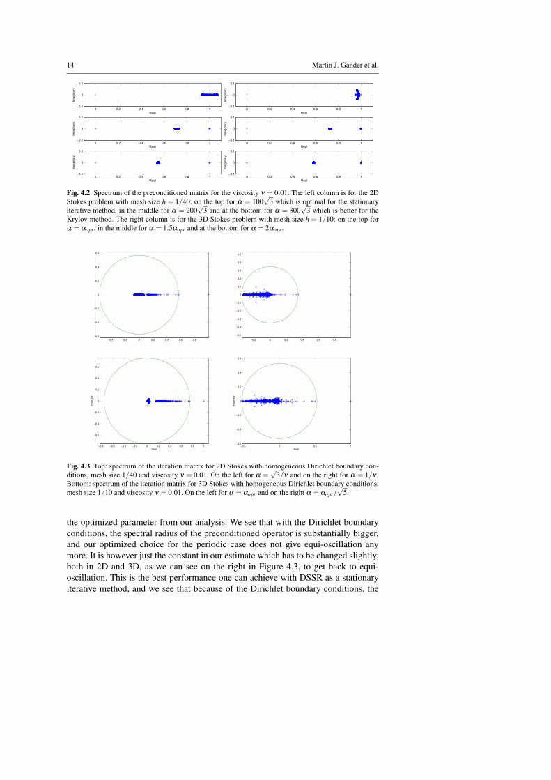
Fig. 4.2 Spectrum of the preconditioned matrix for the viscosity ν = 0.01. The left column is for the 2DStokes problem with mesh size h = 1/40: on the top for α = 100

√3 which is optimal for the stationary

iterative method, in the middle for α = 200√

3 and at the bottom for α = 300√

3 which is better for theKrylov method. The right column is for the 3D Stokes problem with mesh size h = 1/10: on the top forα = αopt , in the middle for α = 1.5αopt and at the bottom for α = 2αopt .

−0.4 −0.2 0 0.2 0.4 0.6 0.8

−0.6

−0.4

−0.2

0

0.2

0.4

0.6

−0.2 0 0.2 0.4 0.6 0.8

−0.5

−0.4

−0.3

−0.2

−0.1

0

0.1

0.2

0.3

0.4

0.5

−0.8 −0.6 −0.4 −0.2 0 0.2 0.4 0.6 0.8 1

−0.6

−0.4

−0.2

0

0.2

0.4

0.6

Real

Ima

gin

ary

−0.5 0 0.5 1−0.6

−0.4

−0.2

0

0.2

0.4

0.6

Real

Ima

gin

ary

Fig. 4.3 Top: spectrum of the iteration matrix for 2D Stokes with homogeneous Dirichlet boundary con-ditions, mesh size 1/40 and viscosity ν = 0.01. On the left for α =

√3/ν and on the right for α = 1/ν .

Bottom: spectrum of the iteration matrix for 3D Stokes with homogeneous Dirichlet boundary conditions,mesh size 1/10 and viscosity ν = 0.01. On the left for α = αopt and on the right α = αopt/

√5.

the optimized parameter from our analysis. We see that with the Dirichlet boundaryconditions, the spectral radius of the preconditioned operator is substantially bigger,and our optimized choice for the periodic case does not give equi-oscillation anymore. It is however just the constant in our estimate which has to be changed slightly,both in 2D and 3D, as we can see on the right in Figure 4.3, to get back to equi-oscillation. This is the best performance one can achieve with DSSR as a stationaryiterative method, and we see that because of the Dirichlet boundary conditions, the


ν 1 0.1 0.01 0.001 0.0001α =√

3/ν 0.5694 0.5694 0.5694 0.5694 0.5694α = 1/ν 0.3492 0.3492 0.3492 0.3492 0.3492

Table 4.2 The spectral radius of the iteration matrix Mα versus the viscosity ν for 2D Stokes and meshsize h = 1/40.

0 50 100 150 200 250 300 35010

15

20

25

30

35

40

α

itera

tions

0 50 100 150 200 250 300 350 400 450 5007.5

8

8.5

9

9.5

10

10.5

11

11.5

12

12.5

α

itera

tions

Fig. 4.4 Number of iterations for 2D Stokes required by the stationary iterative DSSR method (left) andusing DSSR as a preconditioner for GMRES (right) with α = 1/ν (the red star) compared to α =

√3/ν

(the black circle), as well as other choices of the relaxation parameters. The mesh size is h = 1/80 and theviscosity ν = 0.01.

performance will be slower than in the case of periodic boundary conditions or on anunbounded domain.

To investigate if the dependence on ν of the optimized parameter based on Fourieranalysis remains correct also with Dirichlet boundary conditions, and if the DSSRmethod is robust in ν in that case, we show for the fixed mesh size h = 1/40 inTable 4.2 the spectral radii (removing again the pressure mode with eigenvalue 1)depending on a diminishing viscosity ν . We observe again that the spectral radiusdoes not depend on ν for both the optimal choice of the relaxation parameter α∗ =√

3/ν based on Fourier analysis, and the choice with the smaller constant chosenbased on our numerical experiments, α = 1/ν . In both cases, DSSR is a robust solverwhen the viscosity becomes small, and similar results are obtained in 3D.

We next test if the numerically chosen constant α = 1/ν is indeed optimal forDirichlet boundary conditions. To this end, we vary the relaxation parameter α for2D Stokes with 16 samples and calculate for each α the number of iterations requiredby the stationary iterative DSSR method, and using DSSR as preconditioner for GM-RES, see Figure 4.4. This shows that with Dirichlet boundary conditions, the choiceα = 1/ν (the red star) is indeed optimal, and better than our prediction α =

√3/ν

(the black circle) based on Fourier analysis, which could not take Dirichlet boundaryconditions into account.

We next investigate if it is also possible in the case of Dirichlet boundary con-ditions to form two clusters in the spectrum, see Figure 4.5. We observe again thatthe eigenvalues form two clusters, but with the Dirichlet conditions, it is not possibleany more to make the second cluster as tight as we want, and thus the Krylov methodwill not become a direct solver in the presence of Dirichlet conditions. However, one


0 0.2 0.4 0.6 0.8 1 1.2 1.4−0.1

0

0.1

0 0.2 0.4 0.6 0.8 1 1.2 1.4−0.1

0

0.1

0 0.2 0.4 0.6 0.8 1 1.2 1.4−0.1

0

0.1

Imagin

ary

0 0.2 0.4 0.6 0.8 1 1.2 1.4−0.1

0

0.1

0 0.2 0.4 0.6 0.8 1 1.2 1.4−0.1

0

0.1

0 0.2 0.4 0.6 0.8 1 1.2 1.4−0.1

0

0.1

Real

0 0.5 1 1.5−0.1

0

0.1

0 0.5 1 1.5−0.1

0

0.1

0 0.5 1 1.5−0.1

0

0.1

Imagin

ary

0 0.5 1 1.5−0.1

0

0.1

0 0.5 1 1.5−0.1

0

0.1

Real

Fig. 4.5 Left: spectrum of the DSSR preconditioned matrix for 2D Stokes with homogeneous Dirich-let boundary conditions and mesh size h = 1/40 and viscosity ν = 0.01. From the top to bottomα = 100,200,300,400,500,1000. Right: spectrum of the preconditioned matrix for 3D Stokes with homo-geneous Dirichlet boundary condition for mesh size h = 1/10 and viscosity ν = 0.01. From top to bottomα = αno,2αno,4αno,8αno and 16αno with αno = αopt/

√5.

2D Stokes equation: h 1/20 1/40 1/80 1/160 1/320DSSR α = 1/ν 12 12 13 13 14

DSSR α =√

3/ν 20 20 22 23 23DSSRGMRES α = 1/ν 8 8 8 8 9

DSSRGMRES α =√

3/ν 8 8 9 9 93D Stokes equation: h 1/20 1/30 1/40 1/50 1/60

DSSR α = αopt/√

5 22 23 23 24 24DSSR α = αopt 47 49 50 51 51

DSSRGMRES α = αopt/√

5 11 11 11 12 12DSSRGMRES α = αopt 12 12 12 13 13

Table 4.3 Number of iterations required by DSSR for homogeneous Dirichlet conditions for ν = 0.01.

can still benefit from this observation: increasing α does not remarkably result in theincrease of iteration counts for large α , see the right plot in Figure 4.4.

We finally show the number of iterations required by the stationary iterative DSSRmethod, as well as using DSSR as a preconditioner for GMRES in Table 4.3. Wesee that the iteration number does not depend on the mesh size, as predicted by theFourier analysis.

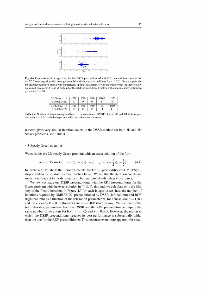
We now compare DSSR with the RDF preconditioner [12]. In Figure 4.6 wesee that for the 2D Stokes problem the spectrum of the DSSR preconditioned ma-trix with the numerically best parameter 1/ν clustered the eigenvalues much fartherfrom the zero eigenvalues than the RDF preconditioned one with experimentally op-timal parameter, which is good for Krylov type solvers. The parameter α∗ from theFourier analysis for the DSSR preconditioner leads to similar result as the RDF pre-conditioner. In Table 4.4 we show the number of iterations required by the RDF pre-conditioner for 2D and 3D Stokes problems with homogeneous Dirichlet boundaryconditions and the viscosity ν = 0.01, where the relaxation parameter is numericallyoptimized. We see that the RDF preconditioner with the numerically optimized pa-


0 0.2 0.4 0.6 0.8 1 1.2 1.4−0.1

−0.05

0

0.05

0.1

0 0.2 0.4 0.6 0.8 1 1.2 1.4−0.1

−0.05

0

0.05

0.1

Imagin

ary

0 0.2 0.4 0.6 0.8 1 1.2 1.4−0.1

−0.05

0

0.05

0.1

Real

Fig. 4.6 Comparison of the spectrum for the DSSR preconditioned and RDF preconditioned matrix forthe 2D Stokes equation with homogeneous Dirichlet boundary conditions for ν = 0.01. On the top for theDSSR preconditioned matrix with numerically optimal parameter 1/ν , in the middle with the theoreticallyoptimized parameter α∗ and at bottom for the RDF preconditioned matrix with experimentally optimizedparameter α = 28.

2D Stokes h 1/20 1/40 1/80 1/160 1/320RDFGMRES 8 9 9 9 93D Stokes h 1/20 1/30 1/40 1/50 1/60RDFGMRES 10 11 11 11 11

Table 4.4 Number of iterations required by RDF preconditioned GMRES for the 2D and 3D Stokes equa-tion with ν = 0.01, with the experimentally best relaxation parameter.

rameter gives very similar iteration counts to the DSSR method for both 2D and 3DStokes problems, see Table 4.3.

4.3 Steady Oseen equation

We consider the 2D steady Oseen problem with an exact solution of the form

u = sinπxsinπy, v = x(1− x)y(1− y), p = (x− 12)(y− 1

2). (4.1)

In Table 4.5, we show the iteration counts for DSSR preconditioned GMRES(20)stopped when the relative residual reaches 1e−6. We see that the iteration counts arerobust with respect to mesh refinement, but increase slowly when ν decreases.

We next compare our DSSR preconditioner with the RDF preconditioner for theOseen problem with the exact solution in (4.1). To this end, we calculate only the fifthstep of the Picard iteration. In Figure 4.7 for each integer α we show the number ofiterations required by GMRES(20) preconditioned by DSSR (left column) and RDF(right column) as a function of the relaxation parameter α , for a mesh size h = 1/80and the viscosity ν = 0.05 (top row) and ν = 0.005 (bottom row). We see that for thebest relaxation parameters, both the DSSR and the RDF preconditioners require thesame number of iterations for both ν = 0.05 and ν = 0.005. However, the region inwhich the DSSR preconditioner reaches its best performance is substantially widerthan the one for the RDF preconditioner. This becomes even more apparent for small


ν = 0.5

Picard Iteration h = 1/20 h = 1/40 h = 1/80 h = 1/1601 10 10 10 102 8 9 9 93 5 5 5 54 2 2 2 25 0 0 0 0

ν = 0.05

1 9 9 10 102 11 11 11 113 9 9 9 94 7 7 7 75 6 6 6 6

ν = 0.005

1 9 9 10 102 21 20 19 193 20 19 18 184 21 19 18 185 19 16 16 16

Table 4.5 Iteration counts for the DSSR preconditioned Oseen problem with exact solution (4.1) for dif-ferent values of the viscosity ν . For the first step we solve a steady Stokes problem with α = 1/ν and inthe following steps the Fourier analyzed relaxation parameter αopt from (3.12) is applied.

4 6 8 10 12 14 16 18 20 22 24 268.5

9

9.5

10

10.5

11

11.5

12

12.5

13

Ite

ratio

ns

α

0 2 4 6 8 10 128.5

9

9.5

10

10.5

11

11.5

12

12.5

13

Ite

ratio

ns

α

15 20 25 30 35 40 45 50 5516.5

17

17.5

18

18.5

19

19.5

20

20.5

21

21.5

22

α

Ite

ratio

ns

8 10 12 14 16 18 20 22 2415.5

16

16.5

17

17.5

18

18.5

19

α

Ite

ratio

ns

Fig. 4.7 Number of iterations required by preconditioned GMRES(20) for the fifth step of a Picard itera-tion for the steady Oseen problem with mesh size h = 1/80 as a function of the relaxation parameter. Theleft column is for the DSSR preconditioner, where the red star indicates the position of the Fourier analysispredicted parameter αopt given by (3.12). The right column is for the RDF preconditioner. The top rowcorresponds to the viscosity ν = 0.05 and the bottom row is for ν = 0.005.


h 1/20 1/30 1/40 1/50 1/60

EXACT

αopt 12 12 12 13 13CPU 2.6347 20.2395 135.0461 620.8271 1786.7771

αopt/√

5 11 11 11 12 12CPU 2.3534 20.7897 110.8607 592.6696 1662.2182

ILU-GMRES

αopt 17 18 18 17 17CPU 0.7925 3.1885 8.1035 15.7264 35.0197

αopt/√

5 15 15 16 16 17CPU 0.6836 2.6189 6.7926 14.5837 31.2215

ILU-PCG

αopt 19 19 18 17 17CPU 0.7018 2.5171 6.4408 11.5749 21.2642

αopt/√

5 15 16 15 15 16CPU 0.6807 2.1094 5.1505 9.7508 18.3849

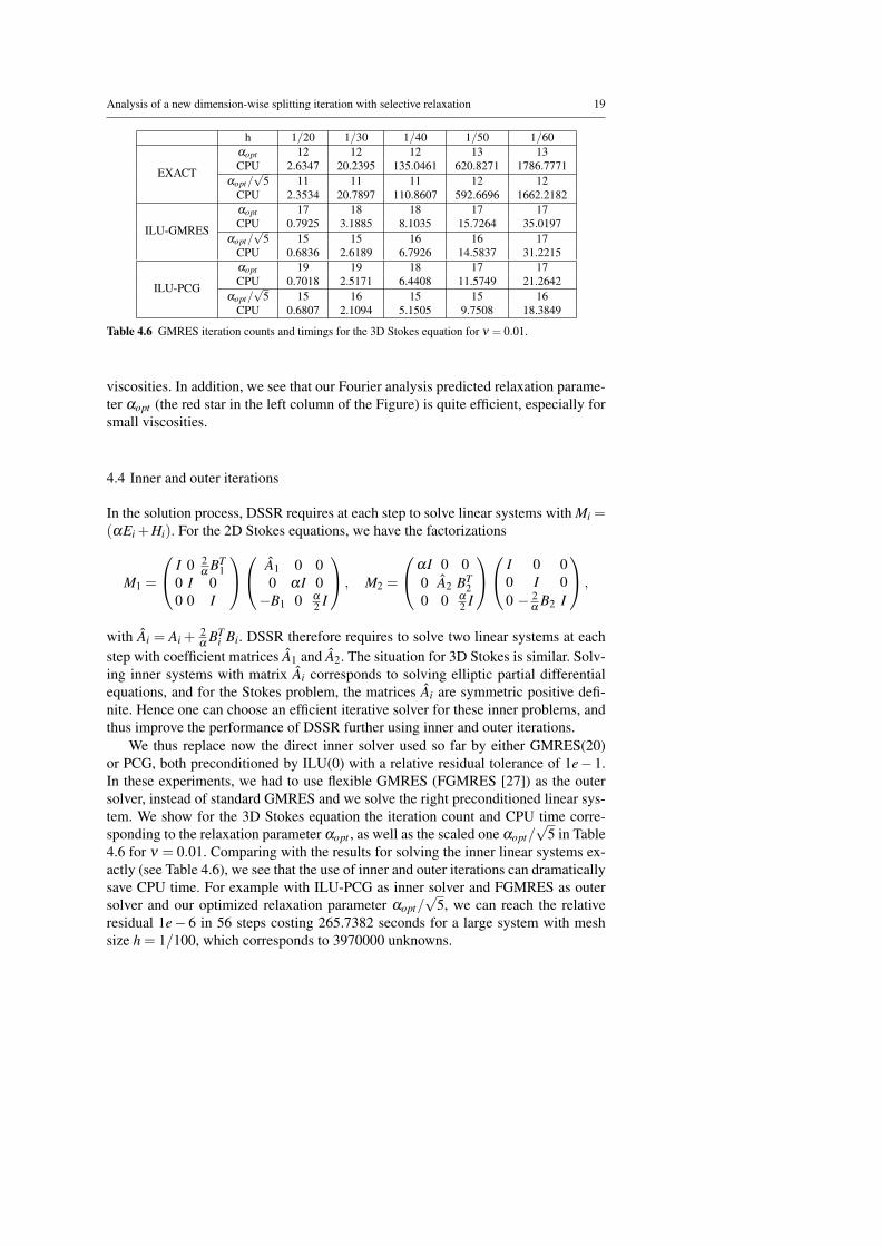
Table 4.6 GMRES iteration counts and timings for the 3D Stokes equation for ν = 0.01.

viscosities. In addition, we see that our Fourier analysis predicted relaxation parame-ter αopt (the red star in the left column of the Figure) is quite efficient, especially forsmall viscosities.

4.4 Inner and outer iterations

In the solution process, DSSR requires at each step to solve linear systems with Mi =(αEi +Hi). For the 2D Stokes equations, we have the factorizations

M1 =

I 0 2α

BT1

0 I 00 0 I

A1 0 00 αI 0−B1 0 α

2 I

, M2 =

αI 0 00 A2 BT

20 0 α

2 I

I 0 00 I 00 − 2

αB2 I

,

with Ai = Ai +2α

BTi Bi. DSSR therefore requires to solve two linear systems at each

step with coefficient matrices A1 and A2. The situation for 3D Stokes is similar. Solv-ing inner systems with matrix Ai corresponds to solving elliptic partial differentialequations, and for the Stokes problem, the matrices Ai are symmetric positive defi-nite. Hence one can choose an efficient iterative solver for these inner problems, andthus improve the performance of DSSR further using inner and outer iterations.

We thus replace now the direct inner solver used so far by either GMRES(20)or PCG, both preconditioned by ILU(0) with a relative residual tolerance of 1e− 1.In these experiments, we had to use flexible GMRES (FGMRES [27]) as the outersolver, instead of standard GMRES and we solve the right preconditioned linear sys-tem. We show for the 3D Stokes equation the iteration count and CPU time corre-sponding to the relaxation parameter αopt , as well as the scaled one αopt/

√5 in Table

4.6 for ν = 0.01. Comparing with the results for solving the inner linear systems ex-actly (see Table 4.6), we see that the use of inner and outer iterations can dramaticallysave CPU time. For example with ILU-PCG as inner solver and FGMRES as outersolver and our optimized relaxation parameter αopt/

√5, we can reach the relative

residual 1e− 6 in 56 steps costing 265.7382 seconds for a large system with meshsize h = 1/100, which corresponds to 3970000 unknowns.


50 100 150 200 250 300 350 400

15

20

25

30

35

40

α

Itera

tion

50 100 150 200 250 300 350 4004

5

6

7

8

9

10

11

α

CP

U T

ime

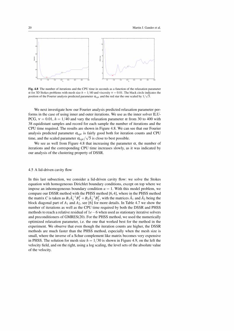
Fig. 4.8 The number of iterations and the CPU time in seconds as a function of the relaxation parameterα for 3D Stokes problems with mesh size h = 1/40 and viscosity ν = 0.01. The black circle indicates theposition of the Fourier analysis predicted parameter αopt and the red star the one scaled by 1/

√5.

We next investigate how our Fourier analysis predicted relaxation parameter per-forms in the case of using inner and outer iterations. We use as the inner solver ILU-PCG, ν = 0.01, h = 1/40 and vary the relaxation parameter α from 30 to 400 with38 equidistant samples and record for each sample the number of iterations and theCPU time required. The results are shown in Figure 4.8. We can see that our Fourieranalysis predicted parameter αopt is fairly good both for iteration counts and CPUtime, and the scaled parameter αopt/

√5 is close to best possible.

We see as well from Figure 4.8 that increasing the parameter α , the number ofiterations and the corresponding CPU time increases slowly, as it was indicated byour analysis of the clustering property of DSSR.

4.5 A lid-driven cavity flow

In this last subsection, we consider a lid-driven cavity flow: we solve the Stokesequation with homogeneous Dirichlet boundary conditions, except on top where weimpose an inhomogeneous boundary condition u = 1. With this model problem, wecompare our DSSR method with the PHSS method [6,4], where in the PHSS methodthe matrix C is taken as B1A−1

1 BT1 +B2A−1

2 BT2 , with the matrices A1 and A2 being the

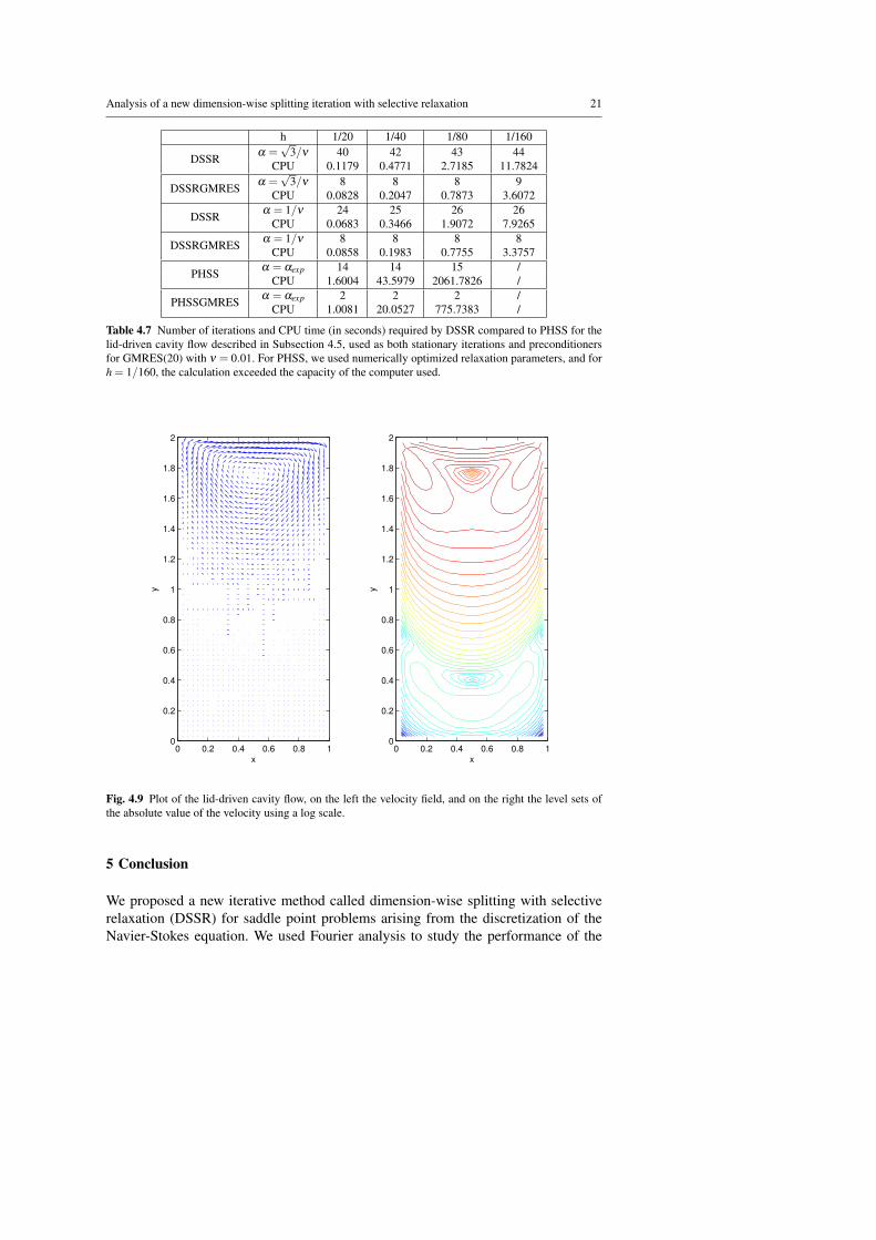
block diagonal part of A1 and A2, see [6] for more details. In Table 4.7 we show thenumber of iterations as well as the CPU time required by both the DSSR and PHSSmethods to reach a relative residual of 1e−6 when used as stationary iterative solversand preconditioners of GMRES(20). For the PHSS method, we used the numericallyoptimized relaxation parameter, i.e. the one that worked best for the method in theexperiment. We observe that even though the iteration counts are higher, the DSSRmethods are much faster than the PHSS method, especially when the mesh size issmall, where the inverse of a Schur complement like matrix becomes very expensivein PHSS. The solution for mesh size h = 1/30 is shown in Figure 4.9, on the left thevelocity field, and on the right, using a log scaling, the level sets of the absolute valueof the velocity.


h 1/20 1/40 1/80 1/160

DSSR α =√

3/ν 40 42 43 44CPU 0.1179 0.4771 2.7185 11.7824

DSSRGMRES α =√

3/ν 8 8 8 9CPU 0.0828 0.2047 0.7873 3.6072

DSSR α = 1/ν 24 25 26 26CPU 0.0683 0.3466 1.9072 7.9265

DSSRGMRES α = 1/ν 8 8 8 8CPU 0.0858 0.1983 0.7755 3.3757

PHSS α = αexp 14 14 15 /CPU 1.6004 43.5979 2061.7826 /

PHSSGMRES α = αexp 2 2 2 /CPU 1.0081 20.0527 775.7383 /

Table 4.7 Number of iterations and CPU time (in seconds) required by DSSR compared to PHSS for thelid-driven cavity flow described in Subsection 4.5, used as both stationary iterations and preconditionersfor GMRES(20) with ν = 0.01. For PHSS, we used numerically optimized relaxation parameters, and forh = 1/160, the calculation exceeded the capacity of the computer used.

0 0.2 0.4 0.6 0.8 10

0.2

0.4

0.6

0.8

1

1.2

1.4

1.6

1.8

2

x

y

x

y

0 0.2 0.4 0.6 0.8 10

0.2

0.4

0.6

0.8

1

1.2

1.4

1.6

1.8

2

Fig. 4.9 Plot of the lid-driven cavity flow, on the left the velocity field, and on the right the level sets ofthe absolute value of the velocity using a log scale.

5 Conclusion

We proposed a new iterative method called dimension-wise splitting with selectiverelaxation (DSSR) for saddle point problems arising from the discretization of theNavier-Stokes equation. We used Fourier analysis to study the performance of the


DSSR iterative method applied to the Stokes and Oseen problems, and obtained opti-mized relaxation parameters, which capture correctly the dependence on the viscosityν also in cases where Fourier analysis is not applicable. The numerical observationthat for the Stokes problem with Dirichlet conditions, the optimized relaxation pa-rameter should be scaled by 1/

√3 in 2D and 1/

√5 in 3D is intriguing, and merits

further investigation.With the asymptotically optimal relaxation parameter, DSSR is robust in the mesh

size h and in ν as well. We have also observed numerically that the performance ofDSSR is comparable to the performance of RDF, but DSSR is more robust in the re-laxation parameter α , and we have an analytical formula for it. The numerical obser-vation that PHSS preconditioned GMRES converges in two steps in our experimentsdeserves further investigation.

A Optimizing θ in DSSR for the Stokes problem

In this appendix we show that θ = 1/2 is the best parameter value for DSSR when applied to the 2D Stokesproblem. Using Fourier analysis as in Subsection 3.1 for the Stokes equation (3.1) with

E1 = diag(0,1,θ), E2 = diag(1,0,1−θ),

one can compute the eigenvalues of the iteration matrix Mα , and we get λ1,2(k1,k2) = 0 and

λ3(k1,k2,θ) =(ανθ(k2

1 + k22)− k2

2)(αν(1−θ)(k21 + k2

2)− k21)

(ανθ(k21 + k2

2)+ k21)(αν(1−θ)(k2

1 + k22)+ k2

2).

We then find

limk2→0|λ3(k1,k2,θ)|=

∣∣∣∣αν(θ −1)θ −θ +1αν(θ −1)θ −θ

∣∣∣∣=: ρ10(α,ν ,θ),

limk2→0|λ3(k1,k2,θ)|=

∣∣∣∣ αν(θ −1)θ +θ

αν(θ −1)θ +θ −1

∣∣∣∣=: ρ20(α,ν ,θ).

It is easy to verify that ρ10 decreases monotonically in θ , ρ20 increases monotonically in θ for θ ∈(0,1) and θ = 1/2 solves ρ10 = ρ20. Thus, if θ 6= 1/2 we would find a spectral radius of Mα withmaxk1 ,k2 ρ(k1,k2,ν ,α) ≥ maxρ10,ρ20 > ρ10(α,ν , 1

2 ), which shows that θ = 1/2 is the best value forthe relaxation parameter θ introduced in Section 2.

Acknowledgment

The authors would like to thank the organizing committee for the wonderful conference NASC2014, wherethe authors met each other and started their collaboration on this interesting topic. They are also very thank-ful for the constructive comments of the anonymous referees, which substantially enhanced the content andstructure of this manuscript.

References

1. Bai, Z.-Z.: Optimal parameters in the HSS-like methods for saddle-point problems. Numer. LinearAlgebra Appl. 16(6), 447–479 (2009)

2. Bai, Z.-Z., Golub, G.H.: Accelerated Hermitian and skew-Hermitian splitting iteration methods forsaddle-point problems. IMA J. Numer. Anal. 27(1), 1–23 (2007)

3. Bai, Z.-Z., Golub, G.H., Li, C.-K.: Optimal parameter in Hermitian and skew-Hermitian splittingmethod for certain two-by-two block matrices. SIAM J. Sci. Comput. 28(2), 583–603 (2006)


4. Bai, Z.-Z., Golub, G.H., Li, C.-K.: Convergence properties of preconditioned Hermitian and skew-Hermitian splitting methods for non-Hermitian positive semidefinite matrices. Math. Comp.76(257),287–298(2007)

5. Bai, Z.-Z., Golub, G.H., Ng, M.K.: Hermitian and skew-Hermitian splitting methods for non-Hermitian positive definite linear systems. SIAM J. Matrix Anal. Appl. 24(3), 603–626 (2003)

6. Bai, Z.-Z., Golub, G.H., Pan, J.-Y.: Preconditioned Hermitian and skew-Hermitian splitting methodsfor non-Hermitian positive semidefinite linear systems. Numer. Math. 98(1), 1–32(2004)

7. Bennequin, D., Gander, M.J., Halpern, L.: A homographic best approximation problem with applica-tion to optimized Schwarz waveform relaxation. Math. Comp. 78(265), 185–223 (2009)

8. Bennequin, D., Gander, M.J., Gouarin, L., Halpern, L.: Optimized Schwarz waveform relaxation foradvection reaction diffusion equations in two dimensions. Numer. Math. (to appear 2016)

9. Benzi, M., Gander, M.J., Golub, G.H.: Optimization of the Hermitian and skew-Hermitian splittingiteration for saddle-point problems. BIT 43(5), 881–900 (2003)

10. Benzi, M., Golub, G.H., Liesen, J.: Numerical solution of saddle point problems. Acta Numer. 14(1),1–137 (2005)

11. Benzi, M., Guo, X.-P.: A dimensional split preconditioner for Stokes and linearized Navier-Stokesequations. Appl. Numer. Math. 61(1), 66–76 (2011)

12. Benzi, M., Ng, M.K., Niu, Q., Wang, Z.: A relaxed dimensional factorization preconditioner for theincompressible Navier-Stokes equations. J. Comput. Phys. 230(16), 6185–6202 (2011)

13. Brown, P.N., Walker, H.F.: GMRES on (nearly) singular systems. SIAM J. Matrix Anal. Appl. 18(1),37–51 (1997)

14. Cao, Y., Du, J., Niu, Q.: Shift-splitting preconditioners for saddle point problems. J. Comput. Appl.Math. 272, 239–250 (2014)

15. Elman, H.C., Howle, V.E., Shadid, J., Shuttleworth, R., Tuminaro, R.S.: Block preconditioners basedon approximate commutators. SIAM J. Sci. Comput. 27(5), 1651–1668 (2006)

16. Elman, H.C., Howle, V.E., Shadid, J., Silvester, D.J., Tuminaro, R.S.: Least squares preconditionersfor stabilized discretizations of the Navier-Stokes equations. SIAM J. Sci. Comput. 30(1), 290–311(2007)

17. Elman, H.C., Ramage, A., Silvester, D.J.: Algorithm 866: IFISS, a Matlab toolbox for modellingincompressible flow, ACM Trans. Math. Soft. 33(2), 14(2007)

18. Elman, H.C., Tuminaro, R.S.: Boundary conditions in approximate commutator preconditioners forthe Navier-Stokes equations. Electron. Trans. Numer. Anal. 35, 257–280 (2009)

19. Gander, M.J.: Optimized Schwarz methods. SIAM J. Numer. Anal. 44(2), 699–731 (2006)20. Gander, M.J.: Schwarz methods over the course of time. ETNA 31, 228–255 (2008)21. Gander, M.J., Halpern, L.: Optimized Schwarz waveform relaxation for advection reaction diffusion

problems. SIAM J. Numer. Anal. 45(2), 666–697 (2007)22. Gander, M.J., Xu, Y.: Optimized Schwarz methods for circular domain decompositions with overlap.

SIAM J. Numer. Anal. 52(4), 1981–2004 (2014)23. Gander, M.J., Xu, Y.: Optimized Schwarz methods with nonoverlapping circular domain decomposi-

tion. Math. Comp. (to appear 2016)24. Harlow, F.H., Welch, J.E.: Numerical calculation of time-dependent viscous incompressible flow of

fluid with free surface. Physics of fluids 8(12), 2182–2189 (1965)25. Lebedev, V.I.: Difference analogues of orthogonal decompositions, basic differential operators and

some boundary problems of mathematical physics. I. USSR Computational Mathematics and Mathe-matical Physics 4(3), 69–92 (1964)

26. Reichel, L., Ye, Q.: Breakdown-free GMRES for singular systems. SIAM J. Matrix Anal. Appl. 26(4),1001–1021 (2005)

27. Saad, Y.: Iterative Methods for Sparse Linear Systems, SIAM, 2003.28. Welch, J.E., Harlow, F.H., Shannon, J.P., Daly, B.J.: The MAC method-a computing technique for

solving viscous, incompressible, transient fluid-flow problems involving free surfaces. Tech. Rep.,Los Alamos Scientific Lab., Univ. of California, N. Mex. (1965)

Documents

Analysis of a new dimension-wise splitting iteration …gander/Preprints/DSSR.pdfAnalysis of a new dimension-wise splitting iteration with selective relaxation 3 A different idea is