ANALYSIS OF A MULTI TYPE SERVICE OF A NON- MARKOVIAN …

Advances and Applications in Mathematical Sciences Volume 20, Issue 6, April 2021, Pages 975-1001 © 2021 Mili Publications

2010 Mathematics Subject Classification: 05C78.

Keywords: breakdown, delay time, optional vacation.

Received December 10, 2019; Accepted May 15 2020

ANALYSIS OF A MULTI TYPE SERVICE OF A NON-

MARKOVIAN QUEUE WITH BREAKDOWN, DELAY TIME

AND OPTIONAL VACATION

P. MANOHARAN and K. SANKARA SASI

Department of Mathematics

Annamalai University

Annamalainagar-608 002, India

E-mail: [email protected]

[email protected]

Abstract

We consider an 1GM queuing system with k-types of service, random breakdowns, delay

times for repairs to start and a second optional vacation. All arriving customers may choose

either of type j services with probability jp where

k

jj kjp

1.,,3,2,1,1 When the

system becomes empty, the server goes for regular vacation and at the end of the first vacation

the server may take a second optional vacation with .1 pro bability , otherwise he

remains in the system with probability. The system may breakdown at random, its repairs do

not start immediately and there is a delay time. The delay times and the repair times follow a

general distribution. Using supplementary variable technique, we derive the probability

generating function for the number of customers in the system, the average number of

customers in the system and the average waiting time of customers in the system. Particular

case is deduced to check the validity of the present model with already existing models.

Numerical examples are also provided.

1. Introduction

In many examples such as production system, bank services, computer

and communication networks, besides feedback the system have vacation.

Vacation queues with different vacation policies including Bernoulli

schedules, assuming a single vacation policy or multiple vacation policy have


Advances and Applications in Mathematical Sciences, Volume 20, Issue 6, April 2021

976

been studied by many researchers. Levy and Yechiali [12], Fuhrman [9],

Doshi [7] and [8], Keilson and Servi [11], Baba [1], Cramer [6], Borthakur and

Chaudhury [3], Madan [13], [14] and [15], Choi and Park [5], Takagi [18] and

[19], Rosenberg and Yechiali [17] ,Chaudhury [4], Badamchi Zadeh and

Shankar [2] and many others have studied vacation queues with different P.

Manoharan and K. Sankara Sasi vacation policies. Madan and Chaudhury

[16] have studied a single server queue with two phase of heterogeneous

service under Bernoulli schedule and a general vacation time. In this system,

without feedback, the server after completing the service can take vacation

with probability or remain in the system with probability 1 Madan

and Anabosi [15] have studied a single server queue with optional server

vacations based on Bernoulli schedules and a single vacation policy. In this

system, without feedback, the server provides two types of heterogeneous

exponential service and a customer may choose either type of service.

Moreover, the server after completing the service can take vacation with

probability or remain in the system with probability .1

In this paper, we consider an 1GM queuing system with k-types of

service, random breakdowns, delay times for repairs to start and a second

optional vacation. Using supplementary variable technique, we derive the

probability generating function for the number of customers in the system,

the average number of customers in the system and the average waiting time

of customers in the system. The paper is organaized as follows. In section two

the model is described. In section three the distribution of the system is

obtained. In section four the performance measures are calculated. In section

five a particular case is discussed. In section six numerical illustrations are

presented.

2. Model Description

The arrival follows Poisson distribution with mean arrival rate .0

The server provides k-types of service to all arriving customers. Customer

may choose either of type j services with probability jp where

k

j jp1

.1

The service times follows a general distribution, with distribution function

xB j and density function xb j for .,,2,1 kj Further it is assumed

ANALYSIS OF A MULTI TYPE SERVICE OF


977

that dxxj is the conditional probability of completion of the jth service

given that the elapsed service time is x, so that

xB

xbdxx

j

j

j

1

(1)

and therefore

.,,2,1,0

kjexxb

x

j dtt

jj

We assume that the services are mutually independent of each other. Let

kjcBEsBc

jj ,,2,1,1,, denote the Laplace-Stieltjes Transform

(LST) and finite moments of service times respectively. Thus the total time

required by the server to complete a service cycle which may be called as

modified service period is given by

.yprobabilitwith

yprobabilitwith

yprobabilitwith

22

11

kk pB

pB

pB

B

The system may breaks down at random, and the breakdowns are

assumed to occur according to a Poisson stream with mean breakdown rate

.0 Further we assume that once the system breaks down, the customer

whose service is interrupted, comes back to the head of the queue. Once the

system breaks down, its repairs do not start immediately and there is a delay

time. The delay times follow a general (arbitrary) distribution with

distribution function xS and density function .xs Let xdxv be the

conditional probability of a completion of the delay process given that the

delay time is x, so that

xS

xsdxxv

1 (2)

and hence

.0

xdttv

exvxs

Further, the repair times follow a general distribution with distribution

function xG and density function .xg Further it is assumed that dxx

is the conditional probability of the completion of the repair process given



978

that the elapsed repair time is x, so that

xG

xgdxx

1 (3)

and hence

.0

xdtt

exxg

Whenever the system becomes empty, the server goes for a first phase of

regular vacation (FRV) of random length .1V Let xV1 and xv1

respectively denote the distribution function and density function of the first

vacation time. At the end of FRV, the server may take a second optional

vacation (SOV) with probability , otherwise he remains in the system with

probability 1 until a new customer arrives. Let xV 2 and xv 2

respectively denote the distribution function and density function for the SOV

time. Further it is assumed that dxxv i is the conditional probability of the

completion of the ith vacation given that the elapsed vacation time is x, so that

xV

xvdxxv

i

ii

1 (4)

and hence

.2,1;0

iexvxv

x

i dttv

ii

It is also assumed that the vacation times 1V and 2V are mutually

independent of each other having LSTs sV i and finite moments,

.2,1,1, ikVEk

i Thus the total time required to complete the

vacation cycle, which may be called as modified vacation period is given by

.1yprobabilitwith

yprobabilitwith

1

21

V

VV

V

3. System size Distribution

We set up the steady state equations for the stationary queue size

distribution by treating elapsed service time, delay time, repair time, FRV

time and SOV time as supplementary variables. Using these equations, we



979

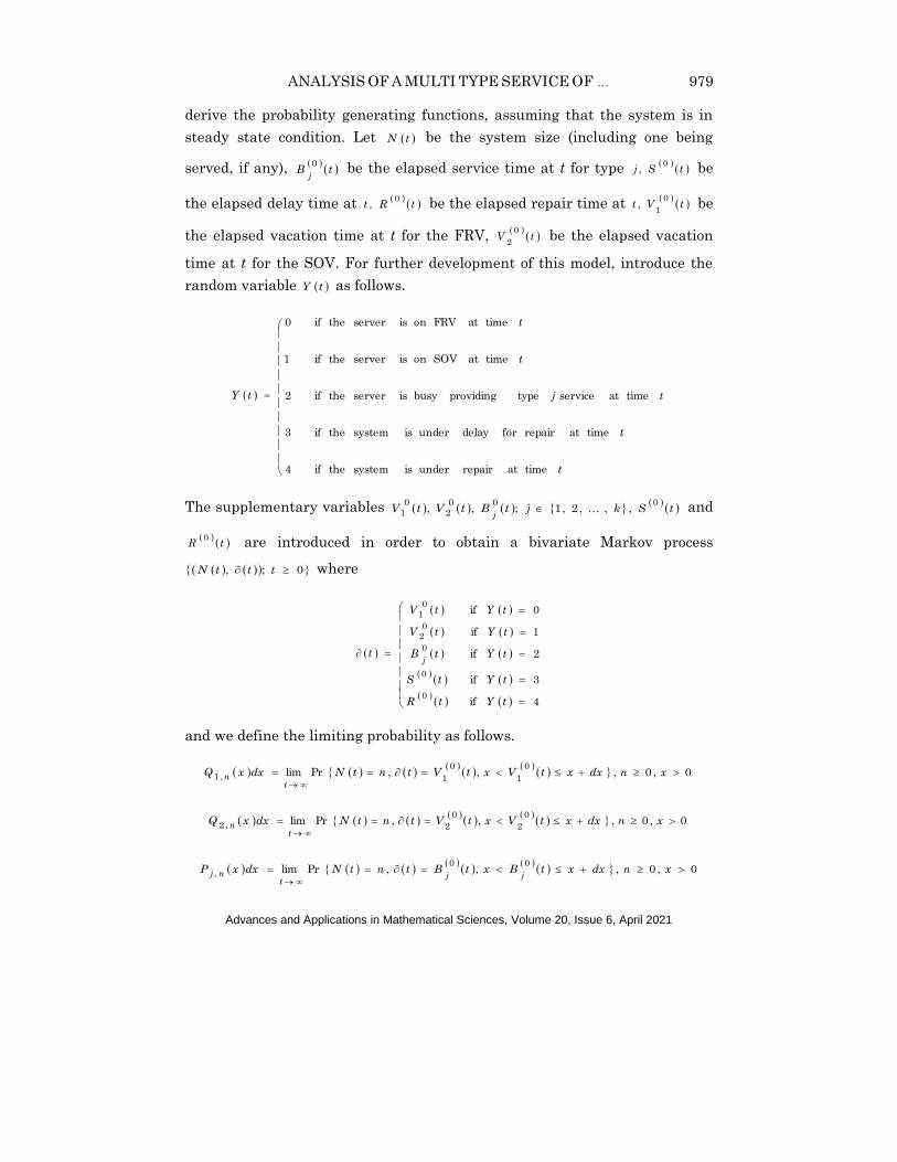
derive the probability generating functions, assuming that the system is in

steady state condition. Let tN be the system size (including one being

served, if any), tB

j

0 be the elapsed service time at t for type tSj

0, be

the elapsed delay time at tRt

0, be the elapsed repair time at

tVt

0

1, be

the elapsed vacation time at t for the FRV,

tV0

2 be the elapsed vacation

time at t for the SOV. For further development of this model, introduce the

random variable tY as follows.

t

t

tj

t

t

tY

time atrepair under is system the if4

time atrepair for delayunder is system the if3

time at service typeproviding busy isserver the if2

time at SOVon isserver the if1

time at FRV on isserver the if0

The supplementary variables

tSkjtBtVtVj

0002

01 ,,,2,1;,, and

tR

0 are introduced in order to obtain a bivariate Markov process

0;, tttN where

4if

3if

2if

1if

0if

0

0

0

02

0

1

tYtR

tYtS

tYtB

tYtV

tYtV

tj

and we define the limiting probability as follows.

0,0,,,Prlim0

1

0

1,1

xndxxtVxtVtntNdxxQt

n

0,0,,,Prlim0

2

0

2,2

xndxxtVxtVtntNdxxQt

n

0,0,,,Prlim00

,

xndxxtBxtBtntNdxxPjj

tnj



980

0,0,,,Prlim00

xndxxtSxtStntNdxxDt

n

.0,0,,,Prlim00

xndxxtRxtRtntNdxxRt

n

Further it is assumed that ,1,00;1,00 SSBB jj

1,00 RR and are continuous at ,0x where 1,00 ii VV

are distribution functions for kj ,,2,1 and 2,1i so that,

xG

xdGdxx

xS

xdSdxxv

xB

xdBdxx

j

j

j

11

;1

and

.

1 xV

xdVdxxv

i

ii

The differential-difference equations governing the system are

kjnxPxPxxPdx

dnjnjjnj ,,2,1,1,1,,, (5)

kjxPxxPdx

dnjjj ,,2,1,0,0, (6)

1,1 nxDxDxvxDdx

dnnn (7)

0,00 xxDdx

d (8)

1,1 nxRxRxxRdx

dnnn (9)

,000 xRxxRdx

d (10)

1,1,1,11,1 nxQxQxvxQdx

dnnn (11)

00,110,1 xQxvxQdx

d (12)

1,1,2,22,2 nxQxQxvxQdx

dnnn (13)



981

,00,220,2 xQxvxQdx

d (14)

k

m

mm dxxxRdxxxPQ

10

00

0,0,1 1

0 0

20,210,1 dxxvxQdxxvxQ (15)

where

.0

0,10,1

dxxQQ

The boundary conditions are

0,10,1 0 QQ (16)

1,00,1 nQ n (17)

0

1,1,2 0,0 ndxxvxQQ nn (18)

k

m

jmmjj dxxxRpdxxxPpP

10 0

11,0, 0

0

11,11 dxxvxQpp jj

0

11,2 ,,2,1 kjdxxvxQp j (19)

k

m

njmnmjnj dxxxRpdxxxPpP

10 0

11,, 0

0

11,11 dxxvxQp nj

0

11,2 ,,2,1 kjdxxvxQp nj (20)



982

k

m

nmn ndxxPD

10

1, 1,0 (21)

000 D (22)

0

1,0 ndxxxDR nn (23)

000 R (24)

and the normalizing condition is

10

1 10

,

n

n

n m

nm dxxRdxxP

0

2

10

,

10

.1

n i

ni

n

n dxxQdxxD (25)

For ,2,1;,,2,1,1;0 ikjzx we define the following

Probability Generating Functions

00

,

0

, ,;,0;,

n

jjnjn

n

jnjn

j dxzxPzPxPzzPxPzzxP

0

00

,;0,0;, dxzxDzDDzzDxDzzxD

n

nn

n

nn

0

00

,;,0;, dxzxRzRxRzzRxRzzxR

n

nn

n

nn

0

0

,

0

, .,;0,0;, dxzxQzQQzzQxQzzxQ i

n

inin

n

inin

i

Multiplying equation (5) by nz and summing from 1n to ∞ and adding

the resultant with equation (6), we get



983

zxzPzxPxzxPdx

djjjj ,,,

.

,

,

xzzxP

zxPdx

d

jj

j

Integrating the above equation with respect to x between 0 and x, we get

.,0

,0

x

j dttxz

j

je

zP

zxP

From equation (1)

.,,2,1,

1kj

tB

tbdtt

j

j

j


.,,2,1,10

kjxBe j

dttx

j

(26)

Using equation (26) in (25), we get

.,,2,1;1,0, kjexBzPzxPxz

jjj

(27)

Multiplying equation (7) by nz and summing from 1n to ∞ and adding the

resultant with equation (8), we get

zxzDzxDxvzxDdx

d,,,

xvz

zxD

zxDdx

d

,

,


.,0

, 0

xdttvxx

ezD

zxD (28)

From equation (2)

.

1 ts

tsdttv



984


.10

xSe

xdttv

(29)


.1,0,xz

exSzDzxD

(30)

Multiplying equation (9) by nz and summing from 1n to ∞ and adding the

resultant with equation (10), we get

zxRzzxRxzxRdx

d,,,

.

,

,

xzzxR

zxRdx

d


.,0

, 0

xdttxx

ezR

zxR (31)

From equation (3)

.

1 tG

tgdtt


.10

xGe

xdtt

(32)


.1,0,xz

exGzRzxR

(33)



.1,0, 121xx

exVzQzxQ

(34)




985


.1,0, 222xz

exVzQzxQ

(35)

Multiplying equation (17) by nz and summing from 1n to ∞ and using

equation (16), we get

.,0 0,11 QzQ (36)

Multiplying equation (18) by nz and summing from 0n to ∞, we get

.,0,0 112 zVzQzQ (37)

Multiplying equation (20) by 1nz and summing from 1n to ∞ and adding

with z times equation (19), we get

k

m

jmmjj dxxzxRpdxxzxPpzzP

100

,,,0

.,,10

0,1220

11

QpdxxvzxQdxxvzxQp jj (38)


.,0

1

k

m

m zPzzD (39)


0

,,0 dxxvzxDzR (40)

Multiplying equation (27) by xj and integrating over 0 to ∞, we get

.,,3,2,1,,0,0

kjzBzPdxxzxP jjjj

(41)

Multiplying equation (30) by xv and integrating over 0 to ∞, we get



986

.,0,0

zSzDdxxvzxD

(42)

Multiplying equation (33) by x and integrating over 0 to ∞, we get

.,0,0

zGzRdxxzxR

(43)

Multiplying equation (34) by xv1 and integrating over 0 to ∞, we get

.,0, 110

11 zVzQdxxvzxQ

Multiplying equation (35) by xv 2 and integrating over 0 to ∞, we get

.,0, 220

22 zVzQdxxvzxQ

(44)

Integrating equation (27) between 0 and ∞, we get

.,,3,2,1,

1,0 kj

zBzPzP

j

jj

(45)

Integrating equation (9.30) between 0 and ∞, we get

.

1,0

z

zSzDzD (46)


.

1,0

z

zGzRzR (47)


.

1,0

111

z

zVzQzQ (48)


.

1,0

2111

z

zVzVzQzQ (49)



987

Using equations (41) to (44) in equation (38), we get

k

m

m

k

m

jmmjj zGzSzPzpzBzPpzzP

11

.,0,0

.11 0,112 QzVzVp j (50)

Put 1j and 1k in equation (50), we get

zD

QzVzVzpzP

1

0,1121

1

11,0

(51)

where

zzBpzzzD 111

.zGzzSzGzzS

Putting 1j and 2k in equation (50), we get

0,13122111 ,0,0 QzzApzAzPpzAzP (52)

where

zzBpzzzA 111

zGzzSzGzzS

zGzzSzzBzA

22

zGzzS

.11 123

zVzVzA

Putting 2j and 2k in equation (50), we get

0,13221212 ,0,0 QzBpzBzPpzBzP (53)

where

zzBpzzzB 221

zGzzSzGzzS



988

zGzzSzzBzB

12

zGzzS

.11 123

zVzVzB


zBzAppzBzA

zBzAzBzApQzpzP

222111

133220,11

1 ,0

(54)

where

zzzBzAzBzAp 13322

11 12

zVzV (55)

zzzzzBAppzBzA 222111

zzBp 11

zGzSzzGzzS

zzBp 22

.zGzSzzGzzS (56)

Using equations (55) and (56) in equation (54), we get

zD

QxVzVzpzP

2

0,1121

1

11,0

(57)

where

zzBpzBpzzzD 22112

.zGzSzzGzSz


zBzAppzBxA

zAzBzAzBpQzpzP

222111

133210,12

2 ,0

(58)



989

.11 1213321

zVzVzzzAzBzAzBp (59)


.

11,0

2

0,1122

2zD

QxVzVzpzP

(60)

From equations (51), (54) and (60), we get

,

11,0

2

0,112

zD

QxVzVzpzP

j

j

kj ,,2,1 (61)

where

zGzzSzzzzD

3

k

m

mm zGzazSzBp

1

zDz

QzB

zVzVzp

zPj

j

j3

0,1

12

1

11

,

111

3

0,112

zD

QzBzVzVp jj

.,,2,1 kj (62)


k

m

mz

zSzpz

z

zSzDzD

1

11,0

zDz

zVzVzSz

3

12 111



990

k

m

mm QzBp

1

0,1 .1 (63)

Using equations (39), (40), (42) and (62) in equation (47), we get

zDz

zVzVzSzGzzR

3

12 111

k

m

mm QzBp

1

0,1 .1 (64)


.

1

1

0,11

1 Qz

zVzQ

(65)


.

1

1

0,121

2 Qz

zVzVzQ

(66)

Adding equations (62) to (64), we get

k

m

m QzD

zNzRzRzDzP

1

0,14

1 (67)

where

zuzuzuzN 3211

11 121

zVzVzu

zSzGzzzu

12

k

m

mm zBpzu

1

3 1

.34 zDzzD

At zuz 1,1 becomes



991

010011 121

VVu

000112

SGzu

k

m

mm

k

m

mm BpBpu

11

3 111

.01111 3211 uuuN (68)

Differentiating zN 1 with respect to z, we get 11 N and 1"1N as

01111,11111 321323211 uuuuuuuuN

111121111 "32323"21"1 uuuuuuuN

111111112 32"132321 uuuuuuuu

.1112 321 uuu (69)

Differentiating zu1 with respect to z, we get 11 u as

000011 12121

VVVVu

.21 VEVE (70)

Differentiating zu 2 with respect to z, we get 12 u as

000000112

SGSGSGu

.1 SEGE (71)

Using equations (68), (70) and (71) in equation (69), we get

.1121

1

212

"1

k

m

mm BpSEGEVEVEN

At zDz 3,1 and zD 4 becomes

k

m

mm GSBpGSD

1

3 000001

.0011 34 DD



992

Differentiating zD 4 with respect to z, we get 14 D as

001011 334 DDD (72)

Differentiating zD with respect to z, we get 1"D as

.1212011 33"3"4 DDDD (73)

Differentiating zD 3 with respect to z, we get 13 D as

.111

11

3

k

m

mm

k

m

mm BpBpGESED (74)


.1121

11

"4

k

m

mm

k

m

mm BpBpGESED

Putting 1z in equation (67), we get

k

m

m QD

NRDP

1

0,14

1

0

0

1

1111 for m.

Using L’Hospital’s rule, we get

k

m

m QD

NRDP

1

0,14

1

0

0

1

1111 for m.

Again using L’Hospital’s rule, we get

k

m

m QD

NRDP

1

0,1"4

"1

1

1111

.

11

11

0,1

11

1

21

Q

BpBpSEGE

BpSEGEVEVE

k

m

mm

k

m

mm

k

m

mm

Adding equations (65) and (66), we get



993

0,1

1221

1

11Q

z

zVzVzQzQ

0

0121 QQ for m.

So after using L’Hospital’s rule, we get

0,1

121221

1

1Q

zVzVzVzVzQzQ

.11 0,12121 QVEVEQQ (75)

Using the fact that

k

m m QQQRDP1 211 ,1211111 we get

210,1

VEVE

zXQ

(76)

where,

1zX (77)

where

.

11

1

1

k

m

mm

k

m

mm

Bp

BpGESE

(78)


210,1

1

VEVEQ

(79)

and SES

0 is the mean of delay time, SEG

0 is the mean of

repair time, 2211 0,0 VEVVEV are the mean of vacation times

of FRV and SOV respectively. 0,1Q is the steady state probability that the

system is idle due to server’s vacation. Also we have ,1 which is the

stability condition under which steady state solution exists.



994

0,1

1

21 QzD

zNzQzQzRzDzPzP

k

m

m

zGzzzVzVzN

111 12

zzzBpzS

k

m

jj

1

1

zGzzSz

k

m

mm zGzzSzBp

1

zSzzGzzzVzV

11 12

k

m

mm zSzzGzzzBp

1

k

m

mm zGzzSzzBpzzz

1

zGzzS

zzzVzV

1111 12

k

m

mm zzzBp

1

1

,21 zuzu

where

11 121

zVzVzu

k

m

mm zBpzzu

1

2 1

zDzD 3



995

zP is the probability generating function for the number of customers in

the queue.

4. Performance Measures

Let qL and L denote the steady state average queue size and system size

respectively.

Then

1

0,1

1

zz

q QzD

zN

dx

dzP

dx

dL

010011 121

VVu

k

m

mm

k

m

mm BpBpu

11

2 111 (80)

0111 21 uuN

k

m

mm GSBpGSD

1

3 000001

011 3 DD

0,1Q

zD

zN

dz

dL q

at 1z

0,12

Q

zD

zDzNzNzD at 1z

0,12

1

1111Q

D

DNND

0,12

1

1"11"1Q

D

DNND

.

12

1"11"10,12

Q

D

DNND

(81)

Differentiating zN with respect to z, we get 1N as



996

11111 2121 uuuuN

.11 21 uu (82)

Differentiating zN with respect to z, we get 1"N as

11112111" "21212" uuuuuuN

.11211 212"1 uuuu (83)

Differentiating zu1 with respect to z, we get 11 u as

0000011 122111

VVVVVu

.21 VEVE (84)

Differentiating zu1 with respect to z, we get 1"1u as

.21 212

22

12

"1 VEVEVEVEu (85)

Differentiating zu 2 with respect to z, we get 12 u as

k

m

mm Bpu

1

2 11 (86)


.1

1

21

k

m

mm BpVEVEN

Using equations (80), (84), (85) and (86) in equation (83), we get

k

m

mm BpVEVEVEVEN

1

212

22

12

21"

.12 21

1

VEVEBp

k

m

mm

Differentiating zD with respect to z, we get zD as



997

zDzD 3

11 3 DD (87)

zDzD "3"

11" "3DD (88)


.111

11

2

k

m

jj

k

m

mm BpBpGESED

Differentiating zD 3 with respect to z, we get 1"3D as

k

m

mm GESEBpD

1

2"3 1221

22

1 1

2212 GEGESESEBpBp

k

m

k

m

mmmm

.12

1

GESEBp

k

m

mm

(89)


k

m

mm

k

m

mm BpGESEBpD

11

221221"

22

1

2 GEGESESEBp

k

m

mm

GESEBp

k

m

mm

1

12

where 2

22

122

,,, VEVEGESE are the second moments of delay, repair,

FRV and SOV time respectively. L can be obtained using the relation



998

. qLL Using Little’s formula, we obtain ,qW the average waiting time

in the queue and W, the average waiting time in the system, as

q

q

LW and

LW respectively.

5. Particular case

If there is only one service 1k and no breakdown 0 then, we

get

211

12 111

VEVEzBz

zVzVzP

which coincides with the probability generating function obtained by Gautam

Choudhury irrespective of the notations used.

6. Numerical illustration

To illustrate the effect of some parameters on the system performance

measures, we present a numerical example by considering service times and

vacation times as exponentially distributed as follows.

Assuming the values 12,9,3.0,5.0,2.0,3 21321 pppk

1,5,55.0,5.1 21 vvv for the parameters, subject to the stability

condition and varying the values of from 0.43 to 0.53 in steps of 0.01 and

from 1 to 2 in steps of 0.1 we have calculated the values of ,qL the

corresponding graph is drawn in figure 1. From figure-1, one can notice that

the surface displays an upward trend as expected for increasing value of the

arrival rate and SOV probability against the average queue size .qL



999

Figure-1.

We consider service times and vacation times are distributed as Erlang-2

distribution. Assuming the values ,7,3.0,5.0,2.0,3 1321 pppk

1,5,51,1,5,8 2132 vvv for the parameters, subject to the

stability condition and varying the values of from 0.21 to 0.28 in steps of

0.01 and from 1 to 1.14 in steps of 0.02 we have calculated the values of ,qL

the corresponding graph is drawn in Figure-2. From Figure-2, we see that the

surface displays an upward trend as expected for increasing values of the

arrival rate and SOV probability against the average queue size .qL

Figure-2.



1000

References

[1] Y. Baba, On the 1GMX queue with vacation time, Operation Research Letters 5

(1986), 93-98.

[2] A. Badamchi Zadeh and G. H. Shankar, A two phase queue system with Bernoulli

feedback and Bernoulli schedule server vacation, Information and Management Sciences

19 (2008), 329-338.

[3] A. Borthakur and G. Chaudhury, On a batch arrival Possion queue with generalised

vacation, Sankhya Ser.B 59 (1997), 369-383.

[4] G. Chaudhury, An 1GMX queueing system with a set up period and a vaction period,

Questa 36 (2000), 23-28.

[5] B. D. Choi and K. K. Park, The 1GM retrial queue with Bernoulli schedule, Queueing

Systems 7 (1990), 219-228.

[6] M. Cramer, Stationary distributions in a queueing system with vaction times and limited

service, Queueing Systems 4 (1989), 57-68.

[7] B. T. Doshi, Queueing systems with vacations-a survey, Queueing Systems 1 (1986), 29-

66.

[8] B. T. Doshi, Conditional and unconditional distributions for 1GM type queues with

server vacation, Questa 7 (1990), 229-252.

[9] S. Fuhrmann, A note on the 1GM queue with server vactions, Questa 31 (1981), 13-

68.

[10] B. R. K. Kashyap and M. L. Chaudhry, An introduction to Queueing theory, Kingston,

Ontario, 1988.

[11] J. Keilson and L. D. Servi, Oscillating random walk models for 1GG vacation systems

with Bernoulli schedules, Journal of Applied Probability 23 (1986), 790-802.

[12] Y. Levi and U. Yechilai, An sMM queue with server vactions, Infor. 14 (1976), 153-

163.

[13] K. C. Madan, On a 1bMMX queueing system with general vacation times,

International Journal of Information and Management Sciences 2 (1991), 51-61.

[14] K. C. Madan, An 1GM queue with optional deterministic server vacations, Metron, 7

(1999), 83-95. 1GM Feedback queue with two types of service 33

[15] K. C. Madan and R. F. Anabosi, A single server queue with two types of service,

Bernoulli schedule server vacations and a single vacation policy, Pakistan Journal of

Statistics 19 (2003), 331-342.

[16] K. C. Madan and G. Choudhury, A two stage arrival queueing system with a modified

Bernoulli schedule vacation under N-policy, Mathematical and Computer Modelling 42

(2005), 71-85.



1001

[17] E. Rosenberg and U. Yechiali, The 1GMX queue with single and multiple vacations

under LIFO service regime, Operation Research Letters 14 (1993), 171-179.

[18] H. Takagi, Queueing Analysis: A foundation of performance evalution, Vol 1, North

Holland, Amsterdam, 1993.

[19] H. Takagi, Time dependent process of 1GM vacation models with exhaustive service,

Journal of Applied Probability 29 (1992), 418-429.

Documents

ANALYSIS OF A MULTI TYPE SERVICE OF A NON- MARKOVIAN …