Analysis of a 1950-1999 simulation Analysis of a 1950-1999 simulation with prognostic ozone in ARPEGE-Climatwith prognostic ozone in ARPEGE-Climat

Jean-François Royer, Hubert Teysseidre, Jean-François Royer, Hubert Teysseidre, Hervé Douville, Sophie TytecaHervé Douville, Sophie Tyteca

Meteo-France, CNRM, ToulouseMeteo-France, CNRM, Toulouse

• Importance of ozone• Overview the ARPEGE-Climat ozone parameterization• Presentation of the forced simulation• Mean seasonal cycle• Interannual variability• Reproduction of the ozone hole• Conclusions and perspectives

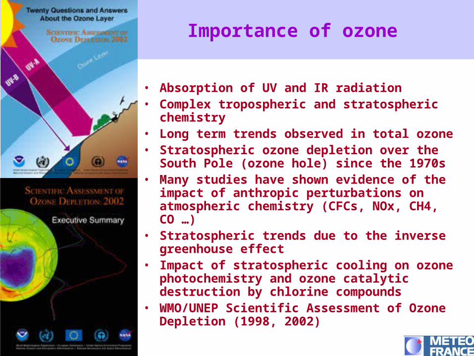
Importance of ozone

• Absorption of UV and IR radiation• Complex tropospheric and stratospheric chemistry• Long term trends observed in total ozone• Stratospheric ozone depletion over the South Pole

(ozone hole) since the 1970s• Many studies have shown evidence of the impact of

anthropic perturbations on atmospheric chemistry (CFCs, NOx, CH4, CO …)

• Stratospheric trends due to the inverse greenhouse effect

• Impact of stratospheric cooling on ozone photochemistry and ozone catalytic destruction by chlorine compounds

• WMO/UNEP Scientific Assessment of Ozone Depletion (1998, 2002)

Purpose of the presentation

• To document the capacity the ARPEGE-Climat GCM, that includes a ozone as a prognostic variable with a simple parameterization of its photochemistry, to reproduce the main characteristics of ozone distribution

• To evaluate its capacity at simulating its observed long term evolution in response to SST, greenhouse gas forcing, and changing composition of the atmosphere

• To identify the impact and signature of anthropic perturbations on the evolution of the ozone layer

Description of the simulations

• ARPEGE-Climat version 3

• Dynamics and resolution:• Semi-lagrangian version with ozone transport• T63 linear grid (128x64 points)• 45 levels in the vertical

• Physical parameterizations• State-of-the-art GCM physics (convective and large-scale

precipitation, interactive clouds, turbulence, land surface processes ISBA)

• ECMWF (Fouquart, Morcrette) radiation scheme (every 3 hours) with major greenhouse gases (CO2, CH4, N20, O3, CFC-11 and CFC-12)

• Sulfate Aerosols: direct and indirect effects (Boucher and Lohman parameterization implemented by Hu RM et al 2002)

• prognostic computation of ozone concentration

The forced simulation

• Aerosols concentrations (J Penner)• The sea surface temperatures (SSTs) are specified according to the

observed monthly means (Reynolds analyses) over the period 1960-2000

• Ozone transport and simplified photochemistry • Derived from the 2D zonal model MOBIDIC

– (MOdel of BI-DImensional Chemistry)

300

310

320

330

340

350

360

370

1950 1960 1970 1980 1990 2000

Year

pp

mv

CO2

1100

1200

1300

1400

1500

1600

1700

1800

1950 1960 1970 1980 1990 2000

Year

pp

bv

CH4

280

290

300

310

320

1950 1960 1970 1980 1990 2000

Year

pp

bv

N2O

0

100

200

300

400

500

600

700

1950 1960 1970 1980 1990 2000

Year

pp

tv

CFC11 CFC12*

•50 year simulation starting in 1950 •Observed GHGs:

•CO2•CH4•N2O•CFC11•CFC12+(others)

Climate statistics

MOBIDICMOBIDICStratosphericStratospheric

chemistrychemistry

Observed SSTs(monthly-mean)

Sea-ice

ISBALand surface

CO2 CH4N2O CFCs

ZonalAverages(10 years)

ARPEGE-ClimatAGCM

Cl

Zonal-mean coefficients for O3 parameterization

Aerosols

The 2D photochemical model MOBIDIC[Cariolle, CNRM, 1984 ; Teyssèdre, UPS, 1994]

• 2 dimensions (latitude, pressure)

• thermodynamical forcings from ARPEGE-Climat (T, v*, w*, Kyy, Kyz, Kzz)

• stratospheric chemistry : 56 species, 175 reactions

• studies of atmospheric impact (supersonic aircraft)

for ozone linear parametrisation :

• chemical equilibrium => (P-L) ; rO3 ; T ;

• +/- 10% perturbation => new equilibrium : (P-L) / rO3 ; (P-L) / T ;

(P-L) /

linearised ozone chemistry[Cariolle and Déqué, JGR, 1986]

rO3 / t = (P-L)

+ (rO3 - rO3

) (P-L) / rO3

+ (T – T) (P-L) / T

+ ( – ) (P-L) /

- Khet (Cly (year))2 rO3

from 3D GCM from 2D photochemical model ( , p)

(P-L) : ozone production-loss term rO3 : ozone mixing ratio

T : temperature : ozone column above gridpoint

Khet : heterogeneous chemistry Cly (year) : total chlorine for given year

(P-L)

rO3 (P-L) / rO3

T (P-L) / T

(P-L) /

Khet (T 195 K under sunlight conditions)

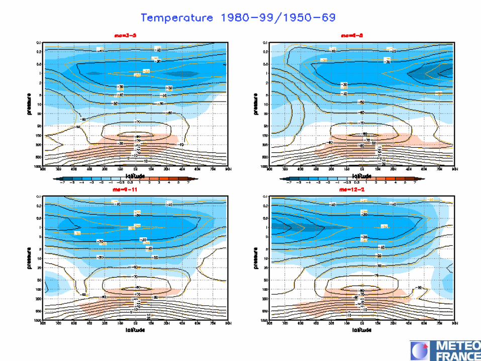
Validation of the resultsComparison of the climate of the 60s and 90s

• Maps of the differences between 20-year mean simulated distributions for two different periods

– 1950-1969

– 1980-1999• Total ozone column (DU= Dobson Units ~ mm O3 at STP)

• Ozone concentration (volume mixing ratio in ppmv)

•Validation of the ozone distribution

–Comparison with UGAMP 5-year ozone climatology 1985-1989

Monthly, 2.5° x 2.5°, 47 levels(Li and Shine, 1995)

Available at BADC

Ozone column (DU) 1985-1989

UGAMP ARPEGE-Climat

Septembre

March

300 400

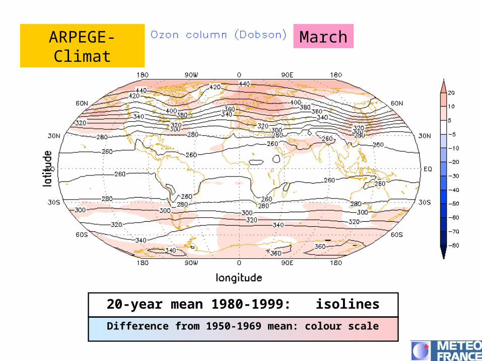
ARPEGE-Climat March

Difference from 1950-1969 mean: colour scale

20-year mean 1980-1999: isolines

Ozone over NH

ARPEGE-Climat

Difference from 1950-1969 mean: colour scale

20-year mean 1980-1999: isolines

September

SPSeptember

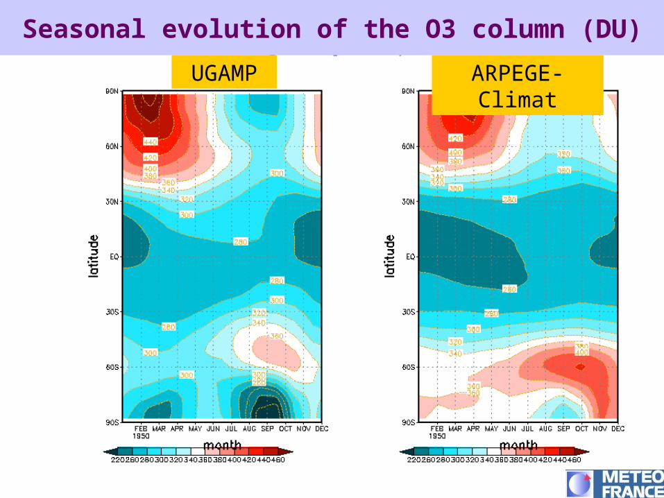
Seasonal evolution of the O3 column (DU)

UGAMP ARPEGE-Climat

Ozone

Difference from 1950-1969 mean: colour scale

20-year mean 1980-1999: isolines

Vertical distribution of O3 concentration (ppmv) 1985-1989

UGAMP ARPEGE-Climat

Annual mean

Seasonal evolution at 10 hPa

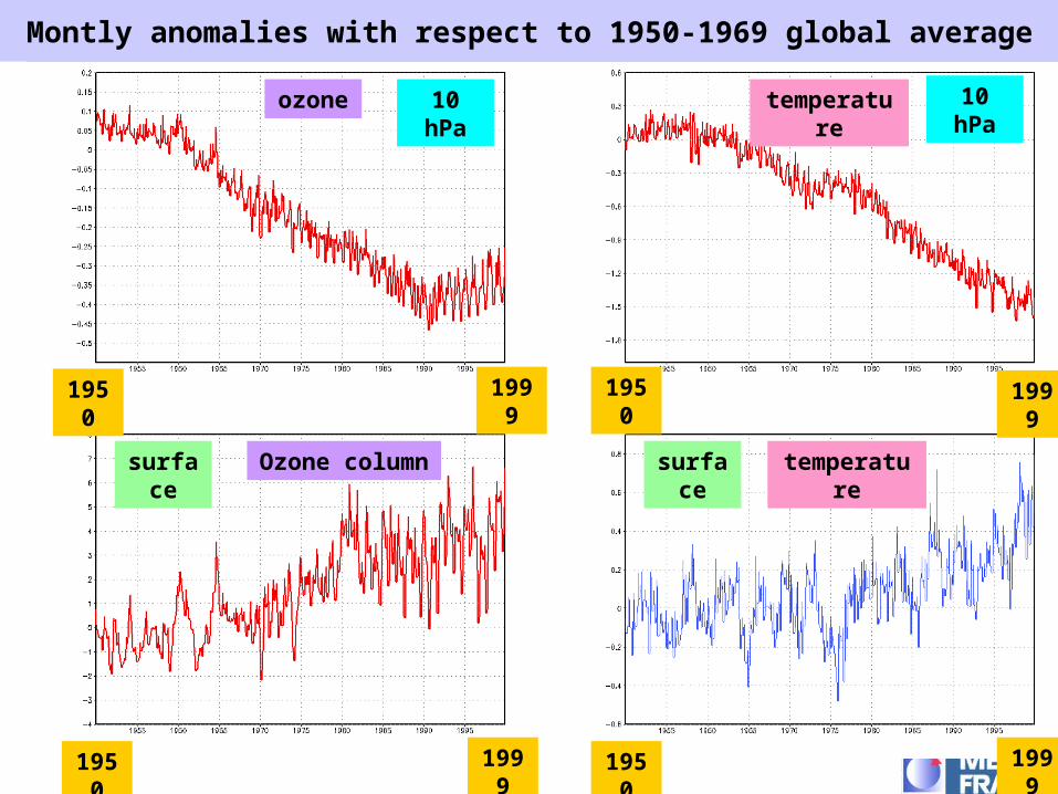
1950 19501999 1999

10 hPa 10 hPa

surface surface

ozone

Ozone column temperature

temperature

Montly anomalies with respect to 1950-1969 global averageMontly anomalies with respect to 1950-1969 global average

1950 19501999 1999

Monthly anomaly with respect to 1950-1969 averagefor ozone column (DU) over South Pole (80-90°S)

Conclusions

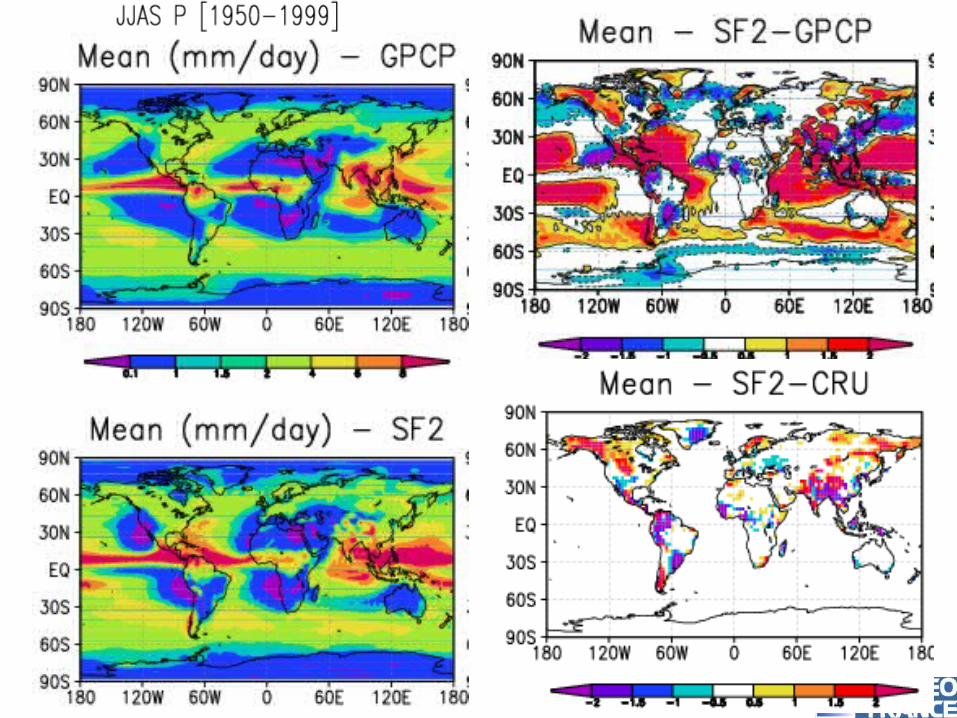
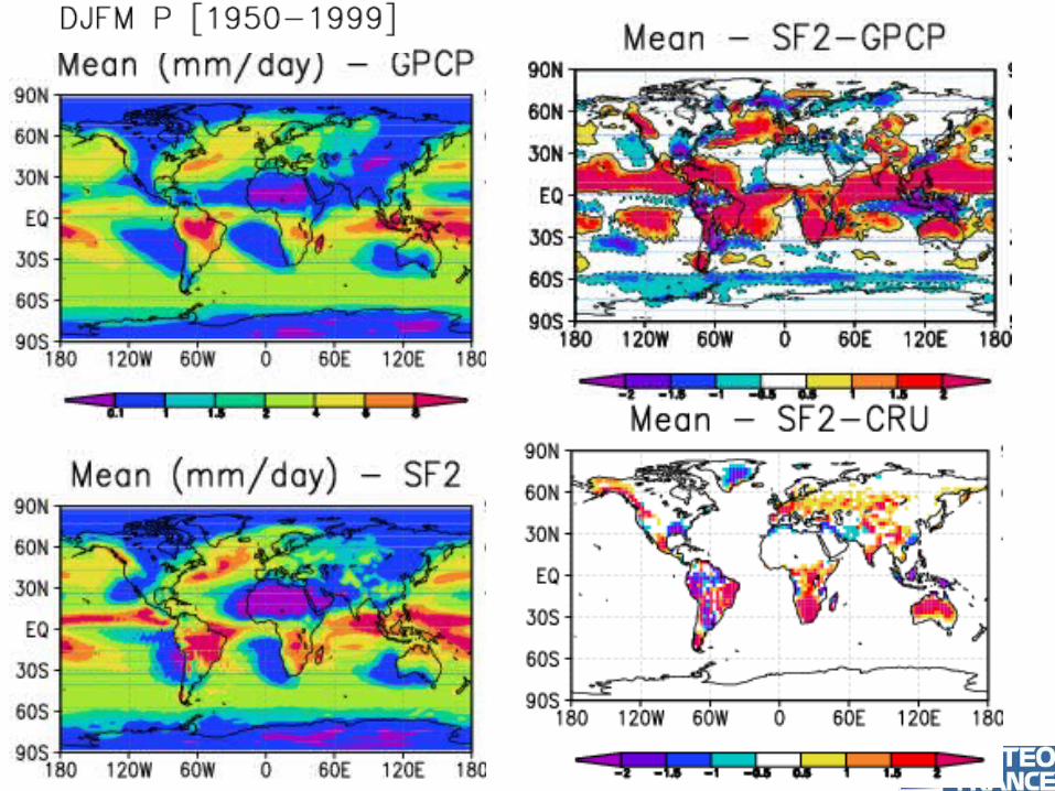
• The ozone transport and simple parameterization of its sources and sinks is able to reproduce the geographical and seasonal distribution patterns of total ozone column

• The vertical distribution of ozone in the stratosphere is simulated realistically

• In response to the increase of CFCs the model simulates a reduction of ozone in the upper stratosphere due to its increased destruction by released chlorine

• This leads to a cooling in the upper stratosphere due to the reduction of UV absorption

• However due to the tropospheric response the total ozone column increases slightly, which is not in agreement with observations

Conclusions (2)

• The heterogeneous chemistry parameterization is able to reproduce the destruction of ozone by PSCs in the South Polar vortex at the begining of Austral spring

• Though the structure of the simulated ozone hole is realistic its intensity is too weak

• Need to revise and adjust the destruction coefficient for heterogeneous chemistry to improve the efficiency of the parameterization in future C20C simulations