Lynchburg CollegeDigital Showcase @ Lynchburg College

Undergraduate Theses and Capstone Projects

Spring 5-1-2018

Analysis of 2016-17 Major League Soccer SeasonData Using Poisson Regression with Rian d. campbellLynchburg College, campbell_i@lynchburg.edu

Follow this and additional works at: https://digitalshowcase.lynchburg.edu/utcp

Part of the Analysis Commons, Applied Statistics Commons, Databases and Information SystemsCommons, Multivariate Analysis Commons, and the Statistical Models Commons

This Thesis is brought to you for free and open access by Digital Showcase @ Lynchburg College. It has been accepted for inclusion in UndergraduateTheses and Capstone Projects by an authorized administrator of Digital Showcase @ Lynchburg College. For more information, please contactdigitalshowcase@lynchburg.edu.

Recommended Citationcampbell, ian d., "Analysis of 2016-17 Major League Soccer Season Data Using Poisson Regression with R" (2018). UndergraduateTheses and Capstone Projects. 59.https://digitalshowcase.lynchburg.edu/utcp/59

i

Analysis of 2016-17 Major League Soccer Season Data Using Poisson

Regression with R

Ian Campbell

Senior Honors Project

Submitted in partial fulfillment of the graduation requirements of the

Westover Honors Program

Westover Honors Program

May 2018

____________________________

Dr. Bahaeddine Taoufik

____________________________

Dr. Kevin Peterson

____________________________

Dr. Nancy Cowden

ii

Abstract

To the outside observer, soccer is chaotic with no given pattern or scheme to

follow, a random conglomeration of passes and shots that go on for 90 minutes. Yet, what

if there was a pattern to the chaos, or a way to describe the events that occur in the game

quantifiably. Sports statistics is a critical part of baseball and a variety of other of today’s

sports, but we see very little statistics and data analysis done on soccer. Of this research,

there has been looks into the effect of possession time on the outcome of a game, the

difference in passing 5 minutes before and after a goal occurred, and very little else. In

this paper, I present an approach to analyze how in game variables contribute to scoring,

and which are more significant to the other. I illustrate the utility of my methods by

applying it to data from the 2016-2017 Major League Soccer (MLS) season collected by

americansocceranalysis.com. This data includes passes, shots on goals, goals themselves,

assists, touch percentage, and much more. By analyzing this data with the statistics

software R and with the use of some descriptive statistics results, boxplots, histograms,

etc. we were able to get multiple representations of how the game is played through

Poisson equations. I explore the concept of separate styles of game play and how the

effect of in game variables changes with these separate styles. The overall goal though is

to find results and hopefully spark an interest into further research and data analysis for

the beautiful game.

iii

Table of Contents Introduction………………………………………………………………............. 1

Literature Review………………………………………………………………… 2

Preliminary Data…………………………………………………………………. 4

Preliminary Results……………………………………………………………… 6

Poisson Distribution……………………………………………………………. 12

Data Analysis …………………………………………………………………... 20

R Analysis……………………………………………………………………….. 24

Adjusted Model…………………………………………………………………. 27

Conclusion ……………………………………………………………………... 34

1

Introduction

Statistics is a branch of the sciences that deals with the collection, analysis, and

interpretation of data. Some believe statistics is a branch of mathematics, but although

statistics depend on mathematics like many other disciplines, math is just a tool used to

solve statistical problems. In today’s world, we wake up and benefit immediately from

daily statistics; we see averages for polls on the news, rainfall on the weather channel,

and hear about our average commute to work over the radio. With so many facets of life

benefitting from statistics, perhaps sports, in general and baseball in particular, have seen

the greatest gain from its use. Every aspect of a baseball player’s profile is defined by

statistics. Whether it’s a pitcher and his earned run average (ERA) that describes how

good he is, or a batter and his weighted on-base average (wOBA) that takes into account

his hits and weights homeruns more than first base hits, players are evaluated by their

stats. Numbers have always dictated baseball, and although sports like football and

basketball don’t see the same dependence on statistics as baseball does, they still receive

statistical support. Yet while these sports receive attention, the most popular sport in the

world is largely ignored by statistical evaluation. Although soccer is not as popular in the

United States as the rest are, the sport could still benefit from the use of statistics. By

evaluating passing schemes, shot patterns, and the overall run of play, statistics could

help coaches identify the aspects of their team's game that could use the most

improvement and what the team already does best; statistical analysis could also help

individual players identify what needs work and what does not. For us as fans, it could

help with winning invaluable arguments against rival fans and maybe help us make a

couple of bucks on the side.

2

As a fan of soccer, the idea of developing a predictive model was immediately

interesting to me. I was interested in using descriptive variables of two teams to create a

model that would predict the outcome of a matchup based on previous results. This

model, if accurate enough, would force teams to improve more effectively, evolving their

game to be less predictable and more innovative. If this trend continued, in the end, the

model would be obsolete, but the goal would be achieved: improving the game of soccer.

Literature Review

Undoubtedly the world’s most popular sport, soccer has seen a considerable

popularity increase in the United States in recent years. However, in a country whose

sports are analyzed all the way down to how many practice swings a batter takes, we

have yet to see the same level of analytics applied to soccer. Analyses that exist right now

for soccer mostly consist of summary statistics, i.e. game-related statistics like goals

scored on each side, possession rates, shots, etc. [1]. These analyses try to distinguish La

Liga (the top professional league in Spain) winning teams from the drawing or losing

ones by use of game-related statistics [5]. Ultimately, Brooks and Kerr took individual

game variables and clustered them together to devise a singular, classifying value. This

value was then compared to other teams’ values, and the results showed that teams are

capable of being characterized by in-game statistics with 70% accuracy. Such analysis is

important because it compares multiple variables, but the model can be improved to

greater than 70% accuracy. Other research done on the Spanish Premier League looked at

which of the game-related statistics allowed us to discriminate among winning, drawing,

and losing teams [7]. We saw that game statistics combined do have a correlation among

3

teams, and now we are able to see which of these factors have the most effect on this

correlation. According to Madarame the biggest distinction in team statistics was that

winning teams made more shots and shots on goal than other teams [7]. Even further,

winning teams were more efficient with shooting as well as passing. What this shows us

is that the most telling attribute of a team is the number of shots they take and how

efficient they are with the shots. This isn't all that surprising, but it certainly wasn't

obvious before evaluating the data. In other terms, we can tell who the better teams are by

looking at the number of goals they score.

Among the research that has been done outside the typical in-game summary

statistics, statistical analysis on the number of goals each team scores is the next most

common measure. They are mostly founded on the number of goals scored or conceded

by each team, and using statistical analysis to show that teams that have been higher

scorers in the past have a greater likelihood of scoring in the future. Sheehan used data

from the English Premier League to this extent, comparing past goals of each team to

build a model that predicts future goal counts [11]. His model confirmed several

important features like home advantage, meaning teams play better (scores more goals) at

home, offensive strengths of each team, and opposition quality. The critical part of

Sheehan’s analysis was his use of the Poisson distribution. A Poisson distribution is a

discrete probability distribution that describes the probability of the number of events

occurring with a specific time period, with the key being the assumption that the number

of events is independent of time [4]. Although Sheehan’s analysis was able to produce a

fairly accurate model for predicting game outcomes, Poisson distributions benefit from a

large number of events, in this case, goals. However, because soccer is a very low-

4

scoring sport, Sheehan was not able to take advantage of this. Using a Poisson

distribution for something like basketball would be much more useful. With the same

concept in mind, a Poisson distribution was applied to the NBA to see if an appropriate

model could be created [8]. What the authors found was that the Poisson distribution was

incredibly accurate, as predicted by the increased number of event occurrences, but only

for a period of time. This is because, in basketball, points made and time are not

independent. As the game nears the end, team game plans change depending on the score,

and points become less frequent, causing the Poisson model to fail. Regardless of this

outcome, it shows us the power of Poisson distribution and its predictive capabilities.

Despite low numbers of scoring events in soccer, there are variables that can be

best used to predict outcomes of games; passing proves to be another key variable, along

with goals scored. Analyses on passing are very limited but include passes per game, pass

locations per game, and passing styles. One analysis shows that teams can be

characterized by where on the pitch they attempt a pass, and teams can be identified by

the number and style of these passes [1]. Using these variables, Brooks and Kerr were

able to achieve a mean accuracy of 87% on predicting which team was which solely

based on passing. Here you need some specific statement about what your project set out

to do. This Project set out to differentiate itself from the previous studies by looking at

input instead of output. By reviewing how goals are scored we can have a better

understanding as how to change and alter the period leading up to a goal to increase the

output. Thus using the statistical software R we were given the opportunity to do just

that. R has the power to evaluate large data sets with methods and equations in an easier,

more condensed, and comprehensible way than other software programs.

5

Preliminary Data

The dataset used in this project was a compilation of player and team statistics,

consisting of variables like shots on goal, passes, and time played for the players and

goals for/against and passes per game for the teams. The data collected originated from

the Major League Soccer (MLS) 2016-2017 season, and although it is very extensive and

consists of 674 of data points, it did not include everything that I needed.

Table 1. Individual player statistics, displaying a sample of the entire data set for

individual player stats.

Players were sorted alphabetically by last name, with their position labeled for

clarification, but sorted by the "Team Cat" column. Each team was given a categorical

variable, i.e., 1 for Chicago Fire and 18 for Real Salt Lake. On top of this, each player

was sorted by position (“Pos. Cat.” column), with “1” referring to an attacking player,

“2” a midfielder, and “3” a defender. For Table 1 the columns in white represent the

original data set, while the ones in yellow are indicators for data columns I created.

Categorical variables were added to compare goals, touch percentage, and assists

between each position as well as each team. "Key Outcomes" in Table 1 refers to a

combination of shots, goals, assists, and key passes, all values that are considered a good

result in the run of play. It is important to note that for key outcomes, I considered shots

and goals equivalent, as well as key passes (passes that led to shots) and assists as

6

equivalent because we cannot account for the skill of the goalkeeper, thus, all of those

events could have been goals or assists if it was a different player.

Table 2. Player Passing Location Data-Sample of the dataset containing passing locations

for individual players.

The second part of the data set included passes made by each player in different

parts of the field. “a.Passes” refers to the attacking third, “m.Passes” the middle, and

“d.Passes” the defense, where “t.Passes” is the total number of passes made by that

player. Originally, this was a part of another data set but was pasted into the first data set

to make it easier to compare variables.

Preliminary Results

Initial research centered on learning the statistical software, R. The software was

critical in the analysis as it allowed for visual representation of the data through

descriptive statistics. Histograms and boxplots played a key role in early analysis,

showing relationships between players, teams, and different positions. Using R to review

the data from Table 1, descriptive statistic tools allowed us to compare our data to data

used in other research and confirm that patterns were similar.

We started by displaying the number of goals for every player in Major League

Soccer using histograms. Doing so showed the distribution of goals, the number of goals

7

with the greatest frequency, and the outliers, i.e., the best goal scorer and how much he

differed from the normal, scoring population.

Figure 1: Key Outcome Distribution-This histogram describes the distribution of key

outcomes per player.

Figure 1 told us that the data are significantly right-skewed, which makes sense:

only the very best players can achieve such high goal values, and there are few superstars

capable of that. We also saw that the maximum number of key outcomes is nearly 200,

whereas the most populated goal range is between 10 and 20. Figure 1 provided a visual

0

20

40

60

0 50 100 150 200

Goals

Co

unt

0

20

40

60

count

Histogram for All Key Outcomes For 2017 MLS PLayers

8

that allowed insight into the players but does not give many other details. Hence, we

sought for further specification on the data presented in Fig. 1. To do this, I included the

categorical variables highlighted in yellow for Table 1. In adding the categorical values

for the players, I opted to not include goalkeepers because many of them have no key

outcomes at all but do have the most playing time, thus skewing the data further. After

categorizing each player, I compared each position’s key outcomes in a series of box

plots to see the difference between the distribution, mean, and outliers of each position.

Figure 2: Key Outcomes Boxplot Distribution-The colored portion of the box plots

indicate the inner 50% of each distribution, while the line is the median of each, and the

dots indicate the outliers.

Interestingly, we see that what would be expected for each position and their key

outcomes. Strikers score the most, then midfield, and finally defenders. What may not be

0

25

50

75

100

125

150

175

200

Attack Mid−Field Defense

Position

Key O

utc

om

es

position

Attack

Mid−Field

Defense

0.7

0.7

Boxplot of mean Key Outcomes per Position

9

an obvious assumption is the distribution for the defenders. We see in Fig. 2 that,

although the median key outcomes for defenders is lower than both midfield and attack,

defenders have a tighter middle range of goals scored, meaning they are more consistent.

Figure 2 also tells us that midfielders may be the most influential position on the field

when it comes to scoring. By looking at the middle range of goals, we see that

midfielders are more consistent than strikers and only have a slightly smaller median.

Furthermore, we know that some of the outliers for midfield are comparable to the

outliers of the strikers.

In order to make a predictive model, it is necessary to look at the distribution of

goals over time for each team. Thus, I created a data set that takes each game played by a

team and counts the number of goals against and goals for, as well as the number of

passes completed, and difference of the number of passes between each team for that

particular game.

10

Table 3. Team Data Per Game-Sample of in game statistics per game for each team

With this data we can see any correlation between the number of passes and the

number of goals or a win. Using R, I displayed the data presented in Table 3 using

separated box plots similar to Fig. 2.

11

Figure 3: Passes Boxplot Distribution-Boxplots show that that there does exist a

difference between number of passes and game outcome.

What we noted was that the average difference in passes per game is higher in

games when teams win than it is when teams lose. By looking at the difference of passes

instead of just normal passes, we can see if teams that are winning also pass more. From

Fig. 3 it is evident that the average for the win is above 0, and the average for the loss is

below zero, meaning that, on average for each winning team, they are passing more than

their opponents. With this outcome, we can apply our understanding to the goals scored

for each team and use it in the Poisson model.

12

With the final direction of the analysis slightly convoluted, I took multiple

approaches to using descriptive statistics with the data. Among these, I compared the best

the worst teams in the MLS and examined the goals scored and conceded.

Figure 4: Best vs. Worst Teams Boxplot Distribution-In this boxplot, looking from left to

right, the first three teams are the best and the last three are the worst.

The best teams in the MLS for the 2016-2017 season were Atlanta United (ATL),

New York FC (NYFC), and Toronto FC (TOR). The worst were the Colorado Rapids

(COL), D.C United (DC), and LA Galaxy (LA). The plot in Fig. 4 shows that each of the

best teams share the attribute that they typically scored more than they conceived, with

each mean goals-for higher than the goals-against mean. For the worst teams, apart from

the Colorado Rapids, the mean of the goals-for was lower than the mean goals-against.

13

After this, I investigated the Poisson distribution as it described the probability of

finding exactly x events in a given period of time, as long as the events occur

independently at a constant rate. Poisson regression is used to predict a dependent

variable that consists of "count data" given one or more independent variables, hence an

excellent model for soccer data.

Poisson Distribution

Named after a French mathematician, Simeon Denis Poisson, the Poisson

distribution is a discrete probability distribution that expresses the probability of a given

number of events occurring in a fixed interval of time or space. For instance, an

individual keeping track of the amount of mail they receive each day may notice that he

receives an average number of four letters per day. If receiving any particular piece of

mail does not affect the arrival times of future pieces of mail, i.e., if pieces of mail from a

wide range of sources arrive independently of one another, then a reasonable assumption

is that the number of pieces of mail received in a day obeys a Poisson distribution.

𝑓(𝑘; 𝜆) = Pr(𝑋 = 𝑘) =𝜆𝑘𝑒−𝜆

𝑘! (1)

Where a discrete random variable X is said to follow a Poisson distribution with

the expected number of occurrences λ>0, if, for k=1,2, 3,… the probability mass function

is given by equation (1) above, where e is Euler's number. The Poisson distribution can

be applied to systems with a large number of possible events, each of which is rare. The

Poisson distribution can answer the question of how many such events can happen in a

fixed time interval, i.e., how many goals will happen in a 90-minute soccer match. For

the use of Poisson, a few assumptions about the dataset are needed.

14

Assumption #1: The dependent variable consists of count data, and count variables

require integer data that must be zero or greater.

Assumption #2: The dataset must have one or more independent variables which can be

measured on a continuous, ordinal or nominal/dichotomous scale.

Assumption #3: The observations are independent. This means that each observation is

independent of the other observations; that is, one observation cannot provide any

information on another observation. This is a critical assumption.

Assumption #4: The mean and variance of the independent variables are the same.

Figure 5: Poisson Example-This figure shows the similarities between an actual

distribution and a predicted distribution when it follows a Poisson distribution.

15

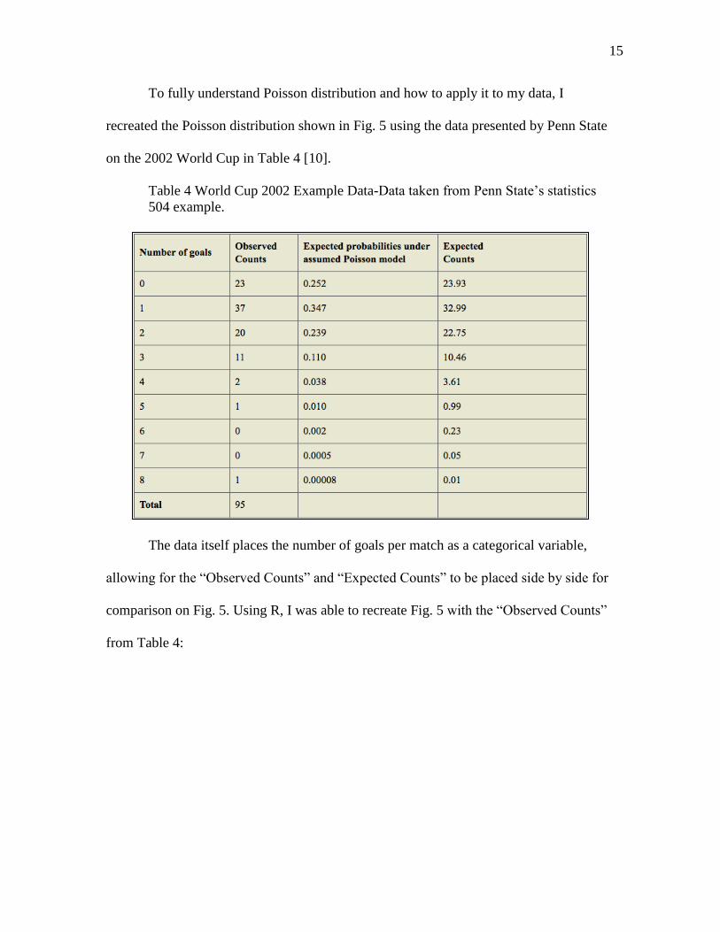
To fully understand Poisson distribution and how to apply it to my data, I

recreated the Poisson distribution shown in Fig. 5 using the data presented by Penn State

on the 2002 World Cup in Table 4 [10].

Table 4 World Cup 2002 Example Data-Data taken from Penn State’s statistics

504 example.

The data itself places the number of goals per match as a categorical variable,

allowing for the “Observed Counts” and “Expected Counts” to be placed side by side for

comparison on Fig. 5. Using R, I was able to recreate Fig. 5 with the “Observed Counts”

from Table 4:

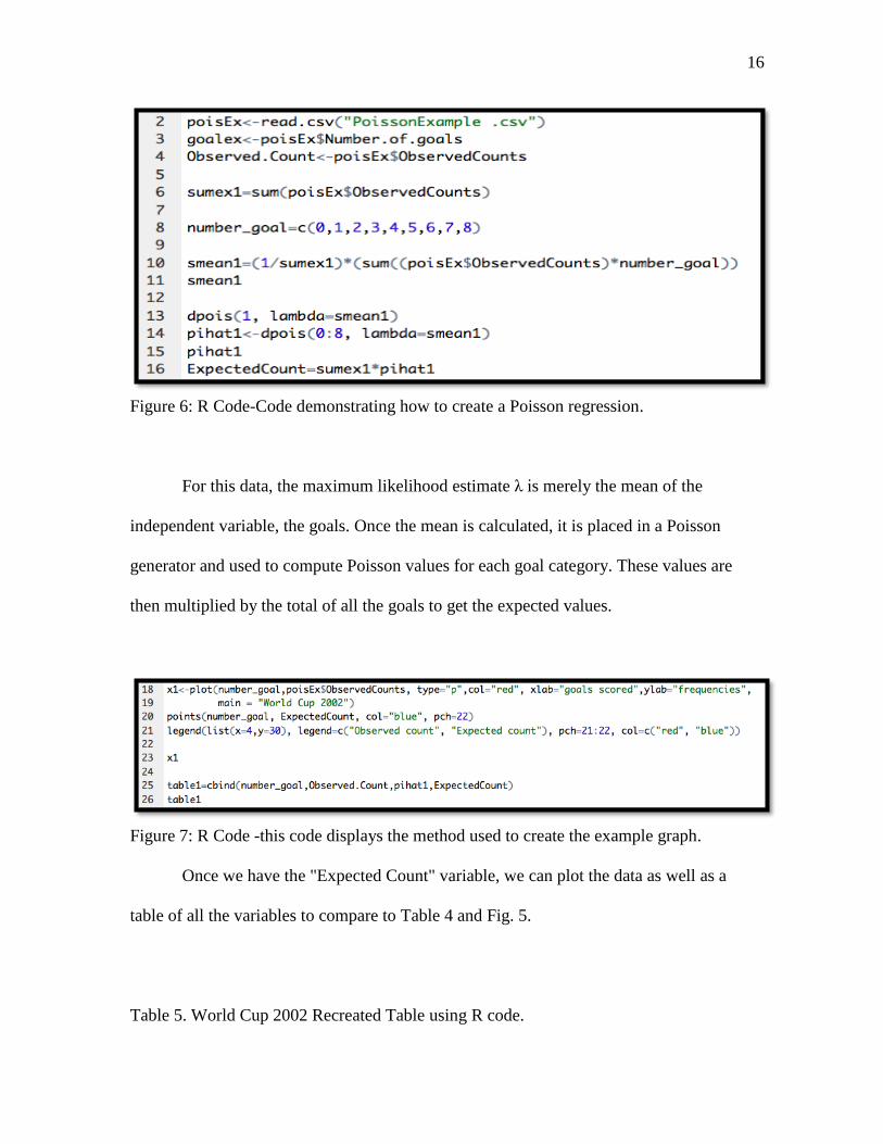
16

Figure 6: R Code-Code demonstrating how to create a Poisson regression.

For this data, the maximum likelihood estimate λ is merely the mean of the

independent variable, the goals. Once the mean is calculated, it is placed in a Poisson

generator and used to compute Poisson values for each goal category. These values are

then multiplied by the total of all the goals to get the expected values.

Figure 7: R Code -this code displays the method used to create the example graph.

Once we have the "Expected Count" variable, we can plot the data as well as a

table of all the variables to compare to Table 4 and Fig. 5.

Table 5. World Cup 2002 Recreated Table using R code.

17

If we compare Tables 4 and 5, we see that the values are exactly the same; the

same applied to Figs. 5 and 6, meaning that I was successfully able to recreate the code

and can, therefore, apply it to my data. Remember that in Poisson it is important to have

the mean and variance of the variable you are using be the same. For this data, the mean

was equal to 1.39, and the variance was equal to 1.65; these values will be important later

on.

18

Figure 8: Recreated World Cup 2002 Plot -This figure compares the example Poisson

data to show the similarities.

MLS 2016-17 Poisson

Since I was successfully able to create the code for Poisson distributions in R, I

applied it to the data presented in Table 6. I first organized the data in Table 1 to a format

similar to that of Table 4 in order to use the code from the example data.

19

Table 6. MLS 2016-2017 Poisson Data-MLS Poisson table using the same methods used

to create Table 5.

At first glance, we see that the “Expected Counts” are similar to the “Observed

Counts,” a good initial indication towards a successful Poisson. Next, we apply the code

to plot and fit the data from Table 6:

Figure 9: This figure shows the code used to recreate the plot shown in Fig. 8.

Then, to visualize the data better, I utilized the R package "GGplot2," to display

the results in a more elegant manner.

20

Figure 10: R Code-The result of the code shown in Fig. 9.

Much like the data displayed in Fig. 6, we see that the "Actual" and the "Poisson"

distributions are incredibly similar, thus leading us to believe that it follows a Poisson

distribution. As stated earlier, the mean and the variance have to be the same in order to

follow a Poisson distribution. So, when we look at the mean and variance, the mean is

equal to 1.48 and the variance 1.62. From the World Cup 2002 example we saw that the

difference between the mean and the variance was 0.27, yet for our data, the difference is

only 0.14. So the data presented here is closer to Poisson than the example but still

violates the assumption of the mean and variance being the same, and since the variance

is more significant than the mean, we have a case of over-dispersion. In order to solve the

issue of over-dispersion, we used the quasi-Poisson model , which is specifically

designed for over-dispersion count data.

21

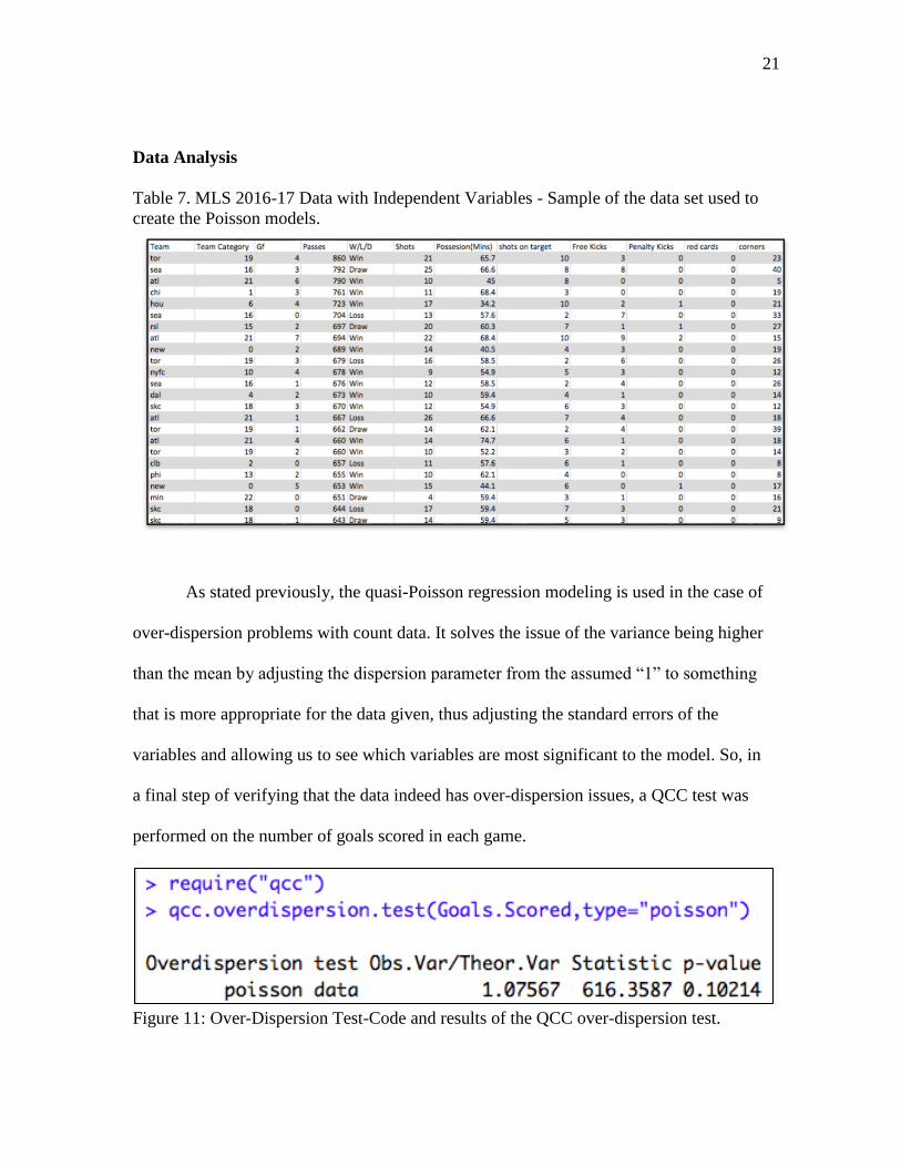
Data Analysis

Table 7. MLS 2016-17 Data with Independent Variables - Sample of the data set used to

create the Poisson models.

As stated previously, the quasi-Poisson regression modeling is used in the case of

over-dispersion problems with count data. It solves the issue of the variance being higher

than the mean by adjusting the dispersion parameter from the assumed “1” to something

that is more appropriate for the data given, thus adjusting the standard errors of the

variables and allowing us to see which variables are most significant to the model. So, in

a final step of verifying that the data indeed has over-dispersion issues, a QCC test was

performed on the number of goals scored in each game.

Figure 11: Over-Dispersion Test-Code and results of the QCC over-dispersion test.

22

The resulting output shows that the p-value is greater than 0.05, meaning that the

data does have over-dispersion issues. With this confirmed, we could finally run the

regression on the number of goals scored in a game. For this regression, I chose eight

different independent variables, shown in Table 7, that I believed would have a

significant effect on the response variable, number of goals. These variables included

passes made (Passes), the amount of time that team possessed the ball during the 90-

minute game (Possesion.Rate), the number of red cards that team received during that

game (Red.Cards), the number of corners taken (Corners), the amount of free kicks taken

(Free.Kicks), the number of penalty kicks taken (Penalty.Kicks), the number of shots

taken (Shots), and the number of shots on target (SoT). Just to clarify, free kicks are those

taken outside the 18-yard box on the opponents’ side of the field, where the defenders are

allowed to stand in front of the ball to obstruct the shooter’s shot, making it harder to

score. Penalty kicks are taken inside the opponents’ 18-yard box, on the 12-yard marker

and is an unobstructed shot between the shooter and the goalkeeper. Also, for this

regression, shots were those that were taken with the intent to score but didn’t always

find the frame of the goal. Shots on target is a subcategory of shots and are those that are

within the frame of the goal, so the categories were treated as two separate variables.

23

Figure 12: Comparison of the distribution of equation variables.

24

As seen in Fig. 8, each variable has few outliers and is either right skewed or normally

distributed. So, with these, I first tested the regression with a normal Poisson distribution

using the code shown below in Fig.13 to see the results before adjusting to the quasi-

Poisson model.

Figure 13: R CodeInitial code used for the Poisson model demonstrating its use.

As can be seen at the bottom of the output, the dispersion parameter is taken to be

1, meaning that it is assuming that the mean and variance are the same, which we've

shown is not the case. Despite this, we still get an interesting look at the variables; on the

right-hand side of the table, the stars indicate the significance of each variable, the more

stars meaning greater significance. These results tell us that before any adjustments are

made, passes, shots, shots-on-target and penalty kicks are the most significant, with free

kicks and red cards as the least significant.

25

R Analysis

Figure 14: R Code-Output of code utilizing quasi-Poisson methods.

What we noticed first is that the dispersion parameter is different; it has been

estimated by R to make the data fit the regression better, thus making the standard errors

modified, specifically, decreasing them. Next, we see that the significance has increased

on all variables except red cards, showing us that they do not affect the goals scored in a

game. This is an astonishing result indeed. Red cards indicate when a person is thrown

out of the game, and in soccer, once a person receives a red card, the team they belong to

is not allowed to replace that person on the field, meaning they are playing a man down, a

definite advantage to the other team. So that would lead me to believe that once a team

receives a red card, their chances to score decrease, but after reviewing the games where

red cards were given out, many of them occurred toward the end of the game. Thus, I

drew the assumption that, because they happened at the end of the game, there was not a

26

significant amount of time for the other team to take advantage of the man down,

therefore rendering the red card a moot point to the score, as shown in the regression.

Also, even though its significance increased, the free kicks variable still does not have

that much effect on the response variable. With this said, we removed both of the

insignificant variables to build the final quasi-Poisson model.

Figure 15: R Code-Adjusted quasi-Poisson model after removing insignificant variables.

The final model indicated that all variables included in the regression were

significant to the model. To better understand what this information means, we can

display it as a linear equation (2).

27

[

ln(𝑦ˆ1)⋮⋮

ln(𝑦ˆ574)

] = [

1 𝑋1,1 𝑋1,2 𝑋1,3 𝑋1,4 𝑋1,5 𝑋1,6

⋮ ⋮ ⋮ ⋮ ⋮ ⋮ ⋮⋮ ⋮ ⋮ ⋮ ⋮ ⋮ ⋮1 𝑋574,1 𝑋574,2 𝑋574,3 𝑋574,4 𝑋574,5 𝑋574,6

]

[ 𝑏0

𝑏1

𝑏2

𝑏3

𝑏4

𝑏5

𝑏6]

(2)

Here, y indicates the goals scored, with the subscript of y indicating the game

number. The variables are denoted as X, with the first number of the subscript being the

game number and the second being the variable number. The estimation coefficients from

the table produced by R are denoted as b, with the subscript being the variable it is related

to. If we wanted to express this equation regarding any single game, it would be as

follows (3):

ln(𝑦ˆ𝑖) = 𝑏0 + 𝑏1𝑋𝑖,1 + 𝑏2𝑋𝑖,2 + 𝑏3𝑋𝑖,3 + 𝑏4𝑋𝑖,4 + 𝑏5𝑋𝑖,5 + 𝑏6𝑋𝑖,6 (3)

Then, if we substitute the variables and estimations from our model, we get our final

equation (4):

ln(𝐺𝑜𝑎𝑙𝑠𝑆𝑐𝑜𝑟𝑒𝑑) = −2.92𝑒−1 + 1.64𝑒−3(𝑃𝑎𝑠𝑠𝑒𝑠) − 1.39𝑒−2(𝑃𝑜𝑠𝑠𝑒𝑠𝑖𝑜𝑛) +

3.81𝑒−2(𝑆ℎ𝑜𝑡𝑠) + 6.23𝑒−2(𝑆𝑜𝑇) − 1.88𝑒−2(𝐶𝑜𝑟𝑛𝑒𝑟𝑠) + 3.24𝑒−1(𝑃𝑒𝑛𝑎𝑙𝑡𝑦𝐾𝑖𝑐𝑘𝑠)

(4)

This equation (4) may at first seem like a mess of numbers, but let me explain what it all

means. If you were to choose one variable and increase it by one unit, i.e., one pass or

one minute of play, while holding all other variables the constant, then if bk>0 for that

variable, there will be an (𝑒𝑏𝑘 − 1)𝑥100% increase on the number of goals scored, y.

Likewise if bk<0 there will be a (1 − 𝑒𝑏𝑘)𝑥100% decrease in the number of goals

scored. For example, for each penalty kick that is taken, a team increases their chance of

28

scoring by 38.38%, while for each minute of possession a team has, their chance of

scoring decreases by 1.38%.

Adjusted Model

As this model serves as a good descriptor of what happens in a soccer game,

solely based off of intuition, it is inherently wrong. For those who are not familiar with

the game of soccer, a penalty kick is highly skewed to be in the favor of the shooter to

score, but let’s review the facts. The shooter is positioned 36 feet from the goal, with the

goal itself being 8 feet tall and 24 feet wide. The average shot speed is around 70 miles

per hour, meaning that it reaches the goal line in about 0.7 seconds, while the average

time it takes the goalkeeper to reach either goal post is 0.6 seconds, meaning that

ultimately the goalie has to make an educated guess. All this put together means that,

barring a shot off-target, the shooter should score a vast majority of the time. So I say the

model is inherently wrong because, as it suggests with the 38.38% increase in the chance

of scoring, the odds are in the favor of the goalkeeper, which as shown, is not the case.

When reviewing the data, in particular the instances where penalties were present,

two realizations were made. First, the sample size is comparably small, consisting of 73

games out of the 574. Second, these 73 games only included penalty kicks that were

scored, not those that were saved as well. Thus, a new data set was created that only

consisted of those games where a penalty kick was taken, including scores and saves,

resulting in a data set with 94 entries.

Table 8. Penalty Kick Data Set-Sample of the data set representing only the games with

penalty kicks taken, the highlighted section representing the target variable.

29

Using this data set, the same method of analysis was conducted to ensure that it

was appropriate for the model. Following the assumptions of Poisson, a QCC test for

over-dispersion was again used to ensure that the data followed the quasi-Poisson model.

Figure 16: Penalty Kick QCC Test Results-R code summarizing the results of the QCC

over-dispersion test.

With a p-value greater than 0.05, the results of the QCC test indicate that the new

data set is indeed over-dispersed, and since the new dataset is a subset of the original, it

satisfies the other three assumptions of the Poisson model, meaning that we are able to

apply the quasi-likelihood model. By following equations 2 and 3, we can apply the code

used in Fig. 15 to the new dataset, with only the final eight variables

30

Figure 17: Penalty Kick Analysis -Output of quasi-Poisson model as applied to the

penalty kicks

Compared to the original analysis, the significance of each value is considerably

less, except for the penalty kicks, which actually increased. We can only speculate on the

cause of the decreases in the significance values, one such speculation is the fact that

these games are different from a normal soccer match. By this I mean for games that

involve penalty kicks, there are significantly more fouls and cards given, meaning that

the games are far more aggressive and, from a player’s point of view, focused less on the

actual soccer aspect of the game. As we can see, the most significant variable is penalty

kicks, with a p-value far less than 0.05, followed by shots on target. Despite having p-

31

values greater than 0.05 and since the model is not representative of the entire set,

variables like shots and corners cannot be excluded from the analysis because we have

already determined that they are significant to the set as a whole. They also provide a

look at what is not significant to games where penalty kicks are present. The important

part of this analysis comes at the bottom of the estimation column in Fig. 18. As

mentioned, this part of the analysis focused on fixing the problem of the low-estimation

coefficient for the penalty kicks corresponding to 38.38%.

ln(𝐺𝑜𝑎𝑙𝑠𝑆𝑐𝑜𝑟𝑒𝑑) = −1.49𝑒−1 + 1.34𝑒−3(𝑃𝑎𝑠𝑠𝑒𝑠) − 2.32𝑒−2(𝑃𝑜𝑠𝑠𝑒𝑠𝑖𝑜𝑛) +

8.17𝑒−3(𝑆ℎ𝑜𝑡𝑠) + 7.77𝑒−2(𝑆𝑜𝑇) − 2.76𝑒−3(𝐶𝑜𝑟𝑛𝑒𝑟𝑠) + 5.95𝑒−1(𝑃𝑒𝑛𝑎𝑙𝑡𝑦𝐾𝑖𝑐𝑘𝑠)

(5)

What equation (5) tells us is that, for those games involving penalty kicks taken,

the chance of scoring increases by 81%; this is calculated using (𝑒𝑏𝑘 − 1)𝑥100% where

bk is the estimated coefficient for penalty kicks (0.595). An 81% increase in the chance of

scoring for every penalty kick taken is a value that makes more sense to me as a player.

This new value takes the favor out of the goalkeeper’s hands and puts it back into the

shooter’s, as it should be.

32

Table 9. MLS 2016-17 dataset excluding penalty kicks.

Since it is evident that games involving penalty kicks and games not involving

penalty kicks are different, its essential to analyze the data set comprising the remaining

482 games where there were no penalty kicks taken. Shown in Table 9, the dataset used

for this distribution has all the same variables, but as shown by the highlighted column,

none of the games had penalty kick occurrences. Since this is another subset of the

original dataset, the first three assumptions about the Poisson regression are met. The last

is met through another QCC over-dispersion test.

Figure 18: QCC Test For Non-Penalty Kick Games-R code summarizing the results of

the QCC over-dispersion test.

With a p-value greater than 0.05 we see that this data is over-dispersed as well,

meaning that we are able to use the quasi-Poisson model. Therefore, we can apply

equations 2 and 3 as well as the code from Fig. 15 to this alternative data set.

33

Figure 19: No Penalty Kick Analysis -Output of quasi-Poisson model as applied to the

non-penalty kick dataset.

As shown in Fig. 19, once the penalty kick variable is removed from the model,

the estimation coefficients and the significance values of the other variables change. The

most significant of these is shots on target, which makes sense considering it was the

second most-significant variable in the original model. Compared to the penalty kick

model, we see a greater emphasis on passes, shots, shots on target, and corners, all

aspects of the game that can be attributed more to actual playing than the aggressive

rugby-style of soccer that was seen with the penalty kick games. The changed estimation

coefficients and significance values also emphasize the differences in game play between

the two distinct types of soccer games. The only insignificant variable, with a p-value

greater than 0.05, is possession rate. This indicates that in the typical game possession

34

does not have an effect on scoring goals; if a team has the ball longer or shorter than the

other, it doesn’t mean that much to the game outcome.

Conclusion

The goal of this project was to offer non-obvious insights into the game of soccer

by using descriptive statistics and analysis in R. This goal was achieved by using Poisson

regression to build models that take in-game variables like shots and passes and places

them into an equation that describes the chances each one offers a team a goal. These

models not only allow me to see what happens to the opportunity of scoring based on

different values for different variables and how significant each one is to scoring but also

indicates how the style of play differs depending on the type of game that is being played.

Based on the significance values computed by R, we see the relative importance of

generating more shots on target and passes for games that do not involve penalty kicks, as

well as possessing the ball and playing aggressively in the box off corners and penalty

kicks for the games do involve penalty kicks.

Moving forward, considering the model shows that an appropriate application of

R and Poisson regression can lead to interesting insights into soccer, I wish to develop the

model further to include other variables. The differences between the two models speaks

to the variability of soccer and that, even though both models serve as good descriptors,

there is always room for improvement. Since each data set is a partial representation of

the original, it can be assumed that it can be further broken down to be more accurate and

provide a better understanding of soccer as a whole. Perhaps breaking down the models

further to include categorical variables like home (home=1) and away (away=0) could

provide a look at how teams play depending on where they are playing. However, soccer

35

is a very complicated sport with ever-changing tactics and situations. Changing the model

to be more team-specific may improve the model to account for an individual team's

characteristics, as it may be the case that a team prefers to possess the ball more, or they

prefer to pass less and attempt more concise attack strategies. Doing this would also

allow us to compare teams and get a more in-depth look at the difference between the

best teams and the worst teams. Lastly, considering this is a more causal model, by this I

mean it's looking the statistics for that game and telling us what the score should have

been based off those variables. It would be interesting to construct a predictive model

using logistic regression that would take the data from previous games and produce a

binary response (1 or 0) that would be a prediction for winning (1) or not winning (0).

Further investigation into this model might show how useful this type of statistical

analysis is to the game of soccer and spark an interest in better understanding this

beautiful game.

36

References

1. Brooks, J., Kerr, M., & Guttag, J. (2016, June 20). Using machine learning to draw

inferences from pass location data in soccer. Vol. 9, Pg. 338-349.

2. Groot, L., & Zoutenbier, M. (2014). The most salient matches in the history of premier

league football. International Journal of the History of Sport, 31(17), 2101-2120.

3. Keller, J. B. (1994). A characterization of the Poisson distribution and the probability

of winning a game. The American Statistician, (4), 294.

4. Lago-Peñas, C., Lago-Ballesteros, J., Dellal, A., & Gómez, M. (2010). Game-related

statistics that discriminated winning, drawing and losing teams from the Spanish

soccer league. Journal of Sports Science & Medicine, 9(2), 288-293.

5. Liu, H., Gomez, M., Lago-Peñas, C., & Sampaio, J. (2015). Match statistics related to

winning in the group stage of 2014 Brazil FIFA World Cup. Journal of Sports

Sciences, 33(12), 1205-1213.

6. Madarame, H. (2017). Game-related statistics which discriminate between winning and

losing teams in Asian and European men's basketball championships. Asian Journal

of Sports Medicine, 8(2), 1-6.

7. Martín-González, J. M., de Saá Guerra, Y., García-Manso, J. M., Arriaza, E., &

Valverde-Estévez, T. (2016). The Poisson model limits in NBA basketball:

Complexity in team sports. Physica A: Statistical Mechanics and its

Applications, 464, 182-190.

37

8. Moura, F. A., Martins, L. E. B., & Cunha, S. A. (2014). Analysis of football game-

related statistics using multivariate techniques. Journal of Sports Sciences, 32(20),

1881-1887.

9. Pennsylvania State University. “2.3.1 - Poisson Sampling.” 2.3.1 - Poisson Sampling

STAT 504, onlinecourses.science.psu.edu/stat504/node/57

10. Sheehan, D. (2017, June 4). Predicting football results with statistical modeling.

Retrieved from https://dashee87.github.io/football/python/predicting-football-

results-with-statistical-modelling/