Embed Size (px)
Citation preview

Modeling, Identification and Control, Vol. 32, No. 1, 2011, pp. 35–45, ISSN 1890–1328
Analysis, Modeling and Simulation of MechatronicSystems using the Bond Graph Method
A. Alabakhshizadeh 1 Y. Iskandarani 2 G. Hovland 2 O. M. Midtgard 1
1Renewable Energy Group, Faculty of Engineering and Science, University of Agder, N-4898 Grimstad, Norway.E-mail: abozar.alabakhshizadeh, [email protected]
2Mechatronics Group, Faculty of Engineering and Science, University of Agder, N-4898 Grimstad, Norway. E-mail:yousef.iskandarani, [email protected]
Abstract
The Bond Graph is the proper choice of physical system used for: (i) Modeling which can be applied tosystems combining multidisciplinary energy domains, (ii) Analysis to provide a great value proposition forfinding the algebraic loops within the system enabling the process of troubleshooting and eliminating thedefects by using the proper component(s) to fix the causality conflict even without being acquainted inthe proper system, and (iii) Simulation facilitated through derived state space equations from the BondGraph model is solved using industrial simulation software, such as 20-Sim, www.20sim.com.
The Bond Graph technique is a graphical language of modeling, in which component energy portsare connected by bonds that specify the transfer of energy between system components. Following a briefintroduction of the Bond Graph methodology and techniques, two separate case studies are comprehen-sively addressed. The first case study is a systematic implementation of a fourth order electrical systemand conversion to mechanical system while the second case study presents modeling of the DielectricElectro Active Polymer (DEAP) actuator. Building the systematic Bond Graph of multifaceted systemand ease of switching between different domains are aims of the first case study while the second studyshows how a complex mechatronic system could be analyzed and built by the Bond Graph. The respectiveBond Graphs in each case is evaluated in the light of mathematical equations and simulations. Excellentcorrelation has been achieved between the simulation results and proper system equations.
Keywords: 20-Sim tool, Bond graph, Casual stroke, Dielectric electro active polymers (DEAP), Pushactuator
1 Introduction
The Bond Graph is an abstract representation of a sys-tem where a collection of components interact witheach other through energy ports and are placed inthe system where energy is exchanged Wong and Rad(1998). The Bond Graph is a graphical method tomodeling and simulation of multi-domain dynamic sys-tems, in which component energy ports are connectedby bonds that specify the transfer of energy betweensystem components. Power, the rate of energy trans-
port between components, is the universal currency ofphysical system Gawthrop and Bevan (2007).
The Bond Graph may be used to model energytransformation across many energy domains includ-ing electrical, mechanical (translation and rotation),hydraulic, thermal, magnetics and chemical. TheBond Graph energy domains for different disciplinesare shown in Table 1.
The Bond Graph takes into consideration both topo-logical and computational structure of multi-domaindynamic systems, while most other graphical tech-
doi:10.4173/mic.2011.1.3 c© 2011 Norwegian Society of Automatic Control
Modeling, Identification and Control
Table 1: Identification of variables Pedersen and Engja (2001)
Energy domain Effort (e) Flow (f) Momentum (p) Displacement (q)
Electrical Voltage [V] Current [A] Flux linkage [Vs] Charge [C]Mechanicaltranslation
Force [N] Velocity [m/s]Linear momentum
[kgm/s]Distance [m]
Mechanicalrotation
Torque [Nm]Angular velocity
[rad/s]Angular
momentum [Nms]Angle [rad]
Hydraulic Pressure [Pa]Volume flow rate
[m3/s]
Pressuremomentum
[N/m2s]Volume [m3]
Thermal Temperature [K] Entropy flow [J/s] - Entropy [J]
MagneticMagneto motive
force [A]Flux rate [Wb/s] - Flux [Wb]
ChemicalChemical potential
[J/mol]Rate of reaction
[mol/s]-
Advancement ofReaction [mol]
niques preserve only topological or computationalstructure. For instance, a circuit diagram reflects thetopological structure of the system while a signal flowgraph and block diagram are used for computationalstructure of the system. These methods are not al-ways applicable to different multi-domain systems; e.g.a circuit diagram is used only for electrical systems.
Some of the advantages of the Bond Graph methodemphasized in the literature are information aboutconstrained states, algebraic loops, and the benefitsand consequences of potential approximations and sim-plifications. Moreover, due to causality assignmentthe method gives the possibility of localization ofstate variables, a tool for finding and removing alge-braic loops and achieving a well-behaved mathematicalmodel. The Bond Graph provides information regard-ing the structural properties of the system, in termsof controllability and observability. Altogether, it isideally suited for modeling and simulation of mecha-tronic systems Khurshid and Malik (2007), Romanet al. (2010).
Although the Bond Graph technique has been in-vented by Professor H. M. Paynter at MIT, approx-imately six decades ago, still it has not been one ofthe main tools for modeling systems. Here, in this pa-per, the Bond Graph technique is introduced, for thefirst time, to the Modeling, Identification and Control(MIC) community. After 30 years of publication, not asingle paper about the Bond Graph has been publishedin MIC.
The paper is organized as follows: (i) Fundamen-tals of the Bond Graph is presented. (ii) Case studyI “Fourth Order Electrical System” is introduced andanalyzed using the Bond Graph and equations are ex-tracted. Then conversion from electrical to mechani-cal domain is accomplished, and the results are proved
with simulation software. (iii) Case study II “DielectricElectro Active Polymer Actuator” is presented, gov-erning equations are derived and explained. The BondGraph model is constructed, and simulation results areshown to match well with the governing output of theequations.
2 Fundamentals of the Bond Graph
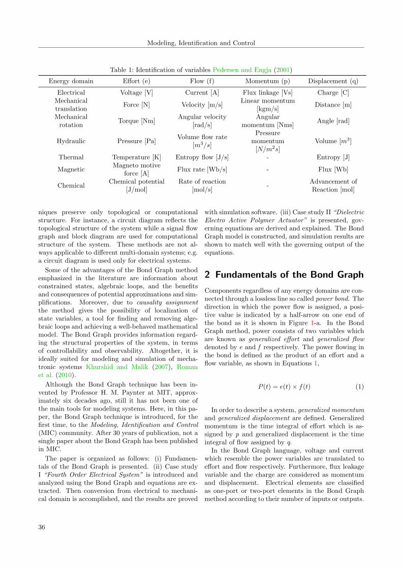
Components regardless of any energy domains are con-nected through a lossless line so called power bond. Thedirection in which the power flow is assigned, a posi-tive value is indicated by a half-arrow on one end ofthe bond as it is shown in Figure 1-a. In the BondGraph method, power consists of two variables whichare known as generalized effort and generalized flowdenoted by e and f respectively. The power flowing inthe bond is defined as the product of an effort and aflow variable, as shown in Equations 1,
P (t) = e(t)× f(t) (1)
In order to describe a system, generalized momentumand generalized displacement are defined. Generalizedmomentum is the time integral of effort which is as-signed by p and generalized displacement is the timeintegral of flow assigned by q.
In the Bond Graph language, voltage and currentwhich resemble the power variables are translated toeffort and flow respectively. Furthermore, flux leakagevariable and the charge are considered as momentumand displacement. Electrical elements are classifiedas one-port or two-port elements in the Bond Graphmethod according to their number of inputs or outputs.
36
A. Alabakhshizadeh et.al, “Mechatronic Systems Modeling using Bond Graph Method”
Figure 1: (a) Sign convention on the power bond. (b)Notation convention for effort and flow re-spect to the indicated causality on a bond
Meaning that, each bond represents two connectionsin the electrical system. For instance resistor, induc-tor, capacitor and sources are considered as one-portelement while transformer is categorized as two-portelement. The common electrical elements and theirrespective Bond Graph and constitutive relations aresummarized in Table 2.
Table 2: Common electrical elements and their properBond Graph indicators and relations
Commonelectricalelements
Bond Graphelement
Constitutiverelations
Voltagesource
See e = e(t)
Currentsource
Sf f
f = f(t)
ResistorefR e = ϕR(f)
e = Rf
InductorefI p = ϕI(f)
p = If
CapacitorefC q = ϕC(e)
q = Ce
Transformere1f1
TFe2f2
e1 = e2mf1m = f2
Gyratore1f1
GYe2f2
e1 = f2rf1r = e2
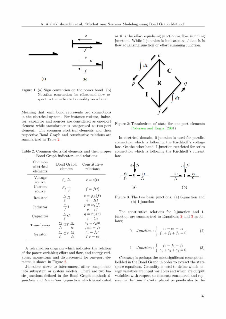
A tetrahedron diagram which indicates the relationof the power variables; effort and flow, and energy vari-ables; momentum and displacement for one-port ele-ments is shown in Figure 2.
Junctions serve to interconnect other componentsinto subsystem or system models. There are two ba-sic junctions defined in the Bond Graph method; 0-junction and 1-junction. 0-junction which is indicated
as 0 is the effort equalizing junction or flow summingjunction. While 1-junction is indicated as 1 and it isflow equalizing junction or effort summing junction.
Figure 2: Tetrahedron of state for one-port elementsPedersen and Engja (2001)
In electrical domain, 0-junction is used for parallelconnection which is following the Kirchhoff’s voltagelaw. On the other hand, 1-junction restricted for seriesconnection which is following the Kirchhoff’s currentlaw.
Figure 3: The two basic junctions. (a) 0-junction and(b) 1-junction
The constitutive relations for 0-junction and 1-junction are summarized in Equations 2 and 3 as fol-lows;
0− Junction :
e1 = e2 = e3
f1 + f2 + f3 = 0(2)
1− Junction :
f1 = f2 = f3
e1 + e2 + e3 = 0(3)
Causality is perhaps the most significant concept em-bedded in the Bond Graph in order to extract the statespace equations. Causality is used to define which en-ergy variables are input variables and which are outputvariables with respect to elements considered and rep-resented by causal stroke, placed perpendicular to the
37
Modeling, Identification and Control
bond at one of its ends. The causal stroke indicatesthe direction of the effort and flow. The direction ofthe causal stroke is independent of the power direction,which is shown in Figure 1-b.
The possible causalities and their respective relationsfor each electrical element are indicated in Table 3.According to Table 3, both voltage and current sourceshave a constant causality while the rest of the elementscould vary between integral and derivative causality.However, the most desirable causality of the storageelements is the integral causality.
Table 3: Common electrical elements and their properBond Graph indicators and causal relations
Commonelectricalelements
BondGraph
element
Causalrelations
Voltagesource
Se | e(t) = given
Currentsource
Sf | f(t) = given
Resistor| R| R
e = ϕR(f)f = ϕ−1
R(e)
Inductor| I| I
e = ddt [ϕI(f)]
f = ϕ−1I (∫edt)
Capacitor| C| C
e = ϕ−1C (∫fdt)
f = ddt [ϕC(e)]
Transformer| TF || TF |
e1 = me2, f2 = mf1e2 = e1
m , f1 = f2m
Gyrator| GY || GY |
e1 = rf2e2 = rf1f1 = ( 1
r )e2f2 = ( 1
r )e1
3 Case Study I
3.1 Electrical Model and Reduced BondGraph Model
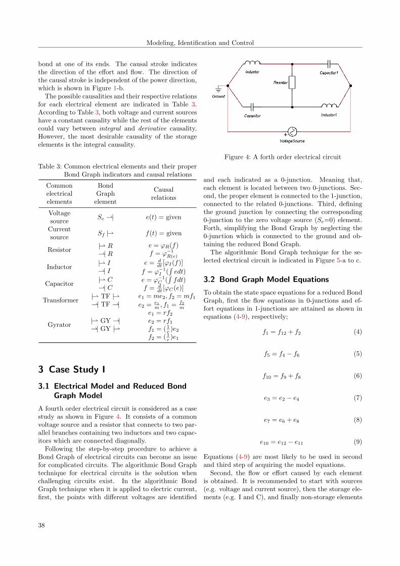
A fourth order electrical circuit is considered as a casestudy as shown in Figure 4. It consists of a commonvoltage source and a resistor that connects to two par-allel branches containing two inductors and two capac-itors which are connected diagonally.
Following the step-by-step procedure to achieve aBond Graph of electrical circuits can become an issuefor complicated circuits. The algorithmic Bond Graphtechnique for electrical circuits is the solution whenchallenging circuits exist. In the algorithmic BondGraph technique when it is applied to electric current,first, the points with different voltages are identified
Figure 4: A forth order electrical circuit
and each indicated as a 0-junction. Meaning that,each element is located between two 0-junctions. Sec-ond, the proper element is connected to the 1-junction,connected to the related 0-junctions. Third, definingthe ground junction by connecting the corresponding0-junction to the zero voltage source (Se=0) element.Forth, simplifying the Bond Graph by neglecting the0-junction which is connected to the ground and ob-taining the reduced Bond Graph.
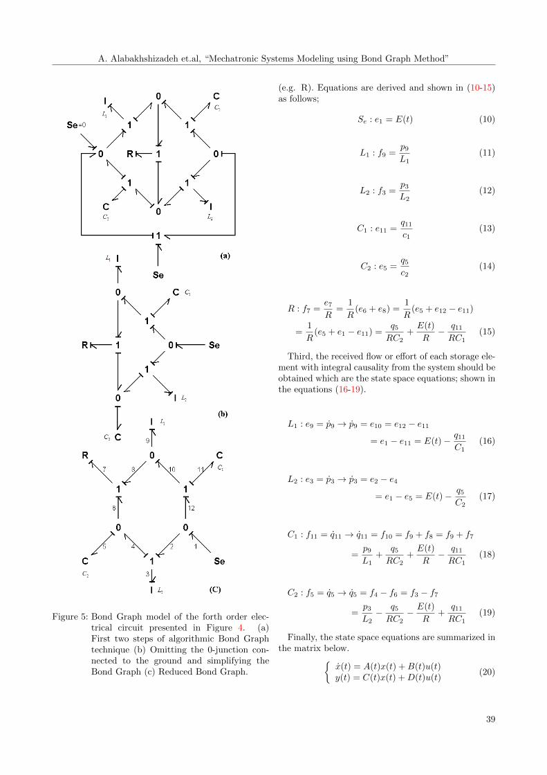
The algorithmic Bond Graph technique for the se-lected electrical circuit is indicated in Figure 5-a to c.
3.2 Bond Graph Model Equations
To obtain the state space equations for a reduced BondGraph, first the flow equations in 0-junctions and ef-fort equations in 1-junctions are attained as shown inequations (4-9), respectively;
f1 = f12 + f2 (4)
f5 = f4 − f6 (5)
f10 = f9 + f8 (6)
e3 = e2 − e4 (7)
e7 = e6 + e8 (8)
e10 = e12 − e11 (9)
Equations (4-9) are most likely to be used in secondand third step of acquiring the model equations.
Second, the flow or effort caused by each elementis obtained. It is recommended to start with sources(e.g. voltage and current source), then the storage ele-ments (e.g. I and C), and finally non-storage elements
38
A. Alabakhshizadeh et.al, “Mechatronic Systems Modeling using Bond Graph Method”
Figure 5: Bond Graph model of the forth order elec-trical circuit presented in Figure 4. (a)First two steps of algorithmic Bond Graphtechnique (b) Omitting the 0-junction con-nected to the ground and simplifying theBond Graph (c) Reduced Bond Graph.
(e.g. R). Equations are derived and shown in (10-15)as follows;
Se : e1 = E(t) (10)
L1 : f9 =p9L1
(11)
L2 : f3 =p3L2
(12)
C1 : e11 =q11c1
(13)
C2 : e5 =q5c2
(14)
R : f7 =e7R
=1
R(e6 + e8) =
1
R(e5 + e12 − e11)
=1
R(e5 + e1 − e11) =
q5RC2
+E(t)
R− q11RC1
(15)
Third, the received flow or effort of each storage ele-ment with integral causality from the system should beobtained which are the state space equations; shown inthe equations (16-19).
L1 : e9 = p9 → p9 = e10 = e12 − e11
= e1 − e11 = E(t)− q11C1
(16)
L2 : e3 = p3 → p3 = e2 − e4
= e1 − e5 = E(t)− q5C2
(17)
C1 : f11 = q11 → q11 = f10 = f9 + f8 = f9 + f7
=p9L1
+q5RC2
+E(t)
R− q11RC1
(18)
C2 : f5 = q5 → q5 = f4 − f6 = f3 − f7
=p3L2− q5RC2
− E(t)
R+
q11RC1
(19)
Finally, the state space equations are summarized inthe matrix below.
x(t) = A(t)x(t) +B(t)u(t)y(t) = C(t)x(t) +D(t)u(t)
(20)
39
Modeling, Identification and Control
p9p3q11q5
=
0 0 − 1
C10
0 0 0 − 1C2
1L1
0 − 1RC1
1RC2
0 1L2
1RC1
− 1RC2
.
p9p3q11q5
+
111R− 1
R
E(t) (21)
e7 =[
0 0 − 1C1
− 1C2
]·
p9p3q11q5
+ E(t) (22)
3.3 Electrical to Mechanical SystemConversion
As mentioned, the main value proposition of the BondGraph technique is its multi-domain characteristics. Inorder to have equivalent systems in different domains,first the Bond Graph should be sketched. Having theBond Graph, it is easy to switch between domains.
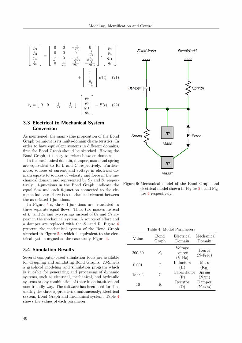
In the mechanical domain, damper, mass, and springare equivalent to R, I, and C respectively. Further-more, sources of current and voltage in electrical do-main equate to sources of velocity and force in the me-chanical domain and represented by Sf and Se respec-tively. 1-junctions in the Bond Graph, indicate theequal flow and each 0-junction connected to the ele-ments indicates there is a mechanical element betweenthe associated 1-junctions.
In Figure 5-c, three 1-junctions are translated tothree separate equal flows. Thus, two masses insteadof L1 and L2 and two springs instead of C1 and C2 ap-pear in the mechanical system. A source of effort anda damper are replaced with the Se and R. Figure 6presents the mechanical system of the Bond Graphsketched in Figure 5-c which is equivalent to the elec-trical system argued as the case study, Figure 4.
3.4 Simulation Results
Several computer-based simulation tools are availablefor designing and simulating Bond Graphs. 20-Sim isa graphical modeling and simulation program whichis suitable for generating and processing of dynamicsystems, such as electrical, mechanical, and hydraulicsystems or any combination of these in an intuitive anduser-friendly way. The software has been used for sim-ulating the three approaches simultaneously; Electricalsystem, Bond Graph and mechanical system. Table 4shows the values of each parameter.
Figure 6: Mechanical model of the Bond Graph andelectrical model shown in Figure 5-c and Fig-ure 4 respectively.
Table 4: Model Parameters
ValueBondGraph
ElectricalDomain
MechanicalDomain
200-60 Se
Voltagesource(V-Hz)
Fource(N-Freq)
0.001 IInductors
(H)Mass(Kg)
1e-006 CCapacitance
(F)Spring(N/m)
10 RResistor
(Ω)Damper(N.s/m)
40

A. Alabakhshizadeh et.al, “Mechatronic Systems Modeling using Bond Graph Method”
Figure 7, shows the simulation results for threeequivalent systems. Voltage applied to the resistor inelectrical model, force applied the damper in the me-chanical model, and R in the Bond Graph model aresketched.
The simulation results show that the obtained BondGraph and mechanical system are equivalent with theelectrical system.
4 Case Study II
4.1 Dielectric Electro Active PolymerActuator
Danfoss PolyPower A/S has been researching into thetechnology of the DEAP for a number of years, usingsmart compliant electrode technology Benslimane et al.(2002) in conjunction with a silicon elastomer WackerChemie AG (2011). So far the company has concen-trated on developing an automatic manufacturing fa-cility for their PolyPower material as well as designingand fabricating PolyPower actuators. Two actuatortypes currently exist; a pre-strained ‘pull’-type actu-ator and a core free tubular ‘push’ actuator with nopre-strain. The surface structure and the electrodes ontheir DEAP film are corrugated. The corrugation al-low the elastomer and the electrodes to be compliant inone direction and stiff in the other direction. Applyingvoltage between the electrodes results in electrostaticforces and contraction between the electrodes. The re-sulting stress from the electro static forces causes theelastomer to elongate in one direction.
A large number of different types of DEAP actuatorshave been demonstrated so far. Most notable examplesinclude planar devices, rolls, tubes, stacks, diaphragmsand extenders. Of the range of DEAP-based actuatorsthat currently exists those having a cylindrical configu-ration (rolls and tubes) are among the most promisingand important. This kind of device was proposed forthe first time by Pelrine et al. (2001), who called it atube actuator. The basic principle of the tube actua-tor is that by applying a voltage to two compliant elec-trodes attached to the internal and external surfaces ofa thin-walled cylindrical dielectric elastomer tube, thetube wall will squeeze, causing an axial elongation.
The spring roll actuator Pelrine et al. (2001), Ash-ley (2003) is perhaps currently the most advancedcylinder-type design for achieving large activationforces with dielectric elastomers. The actuator is com-prised of a bidirectionally pre-stretched and double-side-coated dielectric film wrapped around an elasticcoil spring. The interface for the external fixing of theactuator is made from two threaded rods, which arescrewed from both sides into the coil spring. In or-
der to transmit the forces from the dielectric film tothe spring, the rolled film is glued to the treaded rods.This actuator elongates in the axial direction when avoltage is applied and contracts back to its originallength when deactivated. Elongations up to 26% andforces up to 15 N were achieved at 2500V. This designwas chosen for the dielectric actuators to be used inan arm wrestling robot where 256 spring roll actuatorswith 12 mm outer radius were used.
The actuating performances of the elastomeric di-electric materials, used as electromechanical polymertransducers, have been assessed and continuously im-proved over the last few years so that devices made ofDEAP today represent one of the best smart materialtechnologies using polymer actuation.
This work investigates the PolyPower DEAP actua-tor modeling using the Bond Graph method. The BondGraph representation of the DEAP based actuator isan alternative for the better known block diagram andsignal flow Graph with a major difference of having abidirectional physical energy exchange in between eachof the Bond Graph elements. The work will provide aninsight into (i) the state-of-art Bond Graph modelingof the DEAP push actuator and (ii) the simulation toshow the actuator performances. The following objec-tives are addressed:
• An introduction to the governing equations whichare used for modeling the DEAP push actuator.
• The Bond Graph model of the DEAP actuator.
• The simulations showing (i) Force-Voltage, (ii)Stroke-Voltage and (iii) Force-Stroke relations.
4.2 Governing Equations
Figure 8-a shows the push actuator which is producedby rolling a long laminated sheet of Electro ActivePolymer ‘EAP’ material resulting into multi ‘cylindri-cal’ hollow tube as shown in Figure 8-b.
Figure 8: (a) The DEAP push actuator, (b) (i) Innerand outer pressure when electric field applied(ii) Resultant longitudinal pressure.
These actuators are envisaged to be used as hy-draulic type positioning devices. To model the force
41

Modeling, Identification and Control
Figure 7: Simulation results: Resistor Voltage in Electrical Model (Top), Damper Force in Mechanical Model(Middle), R element effort in Bond Graph (Bottom).
characteristics of the actuator the rolled single EAPlaminated sheet will be approximated as a number ofconcentric cylinders, within the outer and inner radiiof the tubular actuator. Each ‘cylinder’ in the actuatorcontributes to the total force provided by the actuator.Since each cylinder has different geometrical dimen-sion, each of them will contribute a different force tothe overall force ‘Fa’ Iskandarani (2008) which is foundto be:
Fa =ε0 · εr · y · U2
z0(23)
Where ε0 and εr are the dielectric and relative con-stants, y ; the width of the DEAP sheet, z0; the originalthickness, and U ; is the applied voltage.
An applied electrical potential, of opposite signs, oneach of the actuator’s electrodes will cause the elec-trodes to attract each other compressing the cylinderswall thickness. The compression of the wall thicknessresults in elongation of the cylinder as shown in Fig-ure 8-b. The electromechanical model of the strain’S ’ of a cylindrical EAP actuator Iskandarani (2008) isfound to be:
S =2 · ν · FaY ·A
(24)
Where ν and Y represent the Poisson’s ratio andYoung’s modulus of the material and A represents thecross sectional area for the used sheet of material. Theeffective stroke ∆L can be found as follows:
∆L = S · x (25)
Where x is the total length of the actuator and canbe found by summing active and passive length.
It is assumed that the concentric cylinders whichcompose the push actuator are perfectly in contactwith each other such that the outer radius of one cylin-der is equal to the inner radius of the next one. The in-ner and outer circumferences of each cylinder are forcein the material when it is extended. This elastic forceacts in the opposite direction to the actuator force.Since the actuator has to compress the passive part, asshown in Figure 9-a and Figure 9-b, before moving theload it looses some force.
The effective force of a cylindrical EAP actuator con-taining passive parts as shown by Wissler et al. (2007)is reduced as a function of the ratio of the active lengthto the total length as shown in the formula below.
Fe = Fa
(La
La + Lp
)(26)
where Fe is the effective force, La and Lp are activeand the passive actuator length respectively.
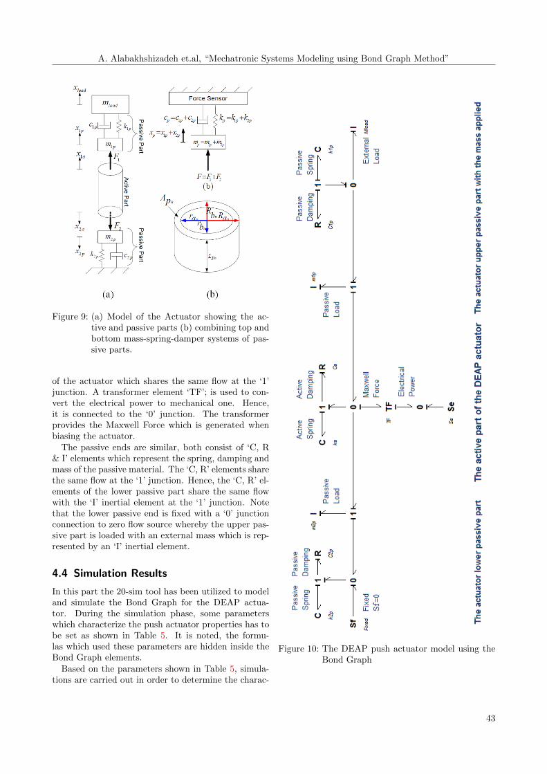
4.3 DEAP with Bond Graph
The graphical representation of the DEAP push actua-tor as shown in Figure 10 has been successfully imple-mented using the Bond Graph. The model has beenimplemented and simulated using the 20-sim software.In the Bond Graph model, the actuator is divided intothree different parts; two passives and one active. Theactive part of the actuator consists of (i) ‘C’; the ac-tive spring component and (ii) ‘R’; the active damping
42
A. Alabakhshizadeh et.al, “Mechatronic Systems Modeling using Bond Graph Method”
Figure 9: (a) Model of the Actuator showing the ac-tive and passive parts (b) combining top andbottom mass-spring-damper systems of pas-sive parts.
of the actuator which shares the same flow at the ‘1’junction. A transformer element ‘TF’; is used to con-vert the electrical power to mechanical one. Hence,it is connected to the ‘0’ junction. The transformerprovides the Maxwell Force which is generated whenbiasing the actuator.
The passive ends are similar, both consist of ‘C, R& I’ elements which represent the spring, damping andmass of the passive material. The ‘C, R’ elements sharethe same flow at the ‘1’ junction. Hence, the ‘C, R’ el-ements of the lower passive part share the same flowwith the ‘I’ inertial element at the ‘1’ junction. Notethat the lower passive end is fixed with a ‘0’ junctionconnection to zero flow source whereby the upper pas-sive part is loaded with an external mass which is rep-resented by an ‘I’ inertial element.
4.4 Simulation Results
In this part the 20-sim tool has been utilized to modeland simulate the Bond Graph for the DEAP actua-tor. During the simulation phase, some parameterswhich characterize the push actuator properties has tobe set as shown in Table 5. It is noted, the formu-las which used these parameters are hidden inside theBond Graph elements.
Based on the parameters shown in Table 5, simula-tions are carried out in order to determine the charac-
Figure 10: The DEAP push actuator model using theBond Graph
43
Modeling, Identification and Control
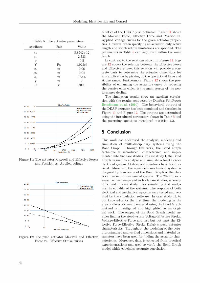
Table 5: The actuator parameters
Attribute Unit Value
ε0 - 8.8542e-12εr - 2.733ν - 0.5Y Pa 1.925e6xa m 0.06xb m 0.04z0 m 75e-6y m 7U V 3000
Figure 11: The actuator Maxwell and Effective Forcesand Position vs. Applied voltage
Figure 12: The push actuator Maxwell and EffectiveForce vs. Effective Stroke curves
teristics of the DEAP push actuator. Figure 11 showsthe Maxwell Force, Effective Force and Position vs.Applied Voltage curves for the given actuator proper-ties. However, when specifying an actuator, only activelength and width within limitations are specified. Theparameters in Table 5 can vary, even within the samebatch.
In contrast to the relations shown in Figure 11, Fig-ure 12 shows the relation between the Effective Forceand Effective Stroke; this relation will provide a con-crete basis to determine the actuator dimensions forany application by picking up the operational force andstroke range. Furthermore, Figure 12 shows the pos-sibility of enhancing the actuators curve by reducingthe passive ends which is the main reason of the per-formance decline.
The simulation results show an excellent correla-tion with the results conducted by Danfoss PolyPowerBenslimane et al. (2010). The behavioral outputs ofthe DEAP actuator has been simulated and sketched inFigure 11 and Figure 12. The outputs are determinedusing the introduced parameters shown in Table 5 andthe governing equations introduced in section 4.2.
5 Conclusion
This work has addressed the analysis, modeling andsimulation of multi-disciplinary systems using theBond Graph. Through this work, the Bond Graphtechnique is introduced, characterized and imple-mented into two case studies. In case study I, the BondGraph is used to analyze and simulate a fourth orderelectrical system. State-space equations have been de-rived. Moreover, the equivalent mechanical system isdesigned by conversion of the Bond Graph of the elec-trical circuit to mechanical system. The 20-Sim soft-ware has been employed in both case studies, wherebyit is used in case study I for simulating and verify-ing the equality of the systems. The response of bothelectrical and mechanical systems were tested and ver-ified by the simulation software. In case study II, toour knowledge for the first time, the modeling in thearea of dielectric smart material using the Bond Graphmethod is investigated and highlighted as an origi-nal work. The output of the Bond Graph model en-ables finding the steady-state Voltage-Effective Stroke,Voltage-Effective Force and last but not least the Ef-fective Force-Effective Stroke DEAP’s push actuatorcharacteristics. Throughout the modeling of the actu-ator, standard and verified dimensions and material pa-rameters have been used for finding the actuator char-acteristics. Moreover, data is collected from practicalexperimentations and used to verify the Bond Graphmodel which concludes accurate correlation.
44
A. Alabakhshizadeh et.al, “Mechatronic Systems Modeling using Bond Graph Method”
Acknowledgment
The work was carried out at the premises of the Univer-sity of Agder, Grimstad. At the University of Agder,appreciative acknowledgments to Professor EmeritusHallvard Engja for his introductory course about theBond Graph as well as for many discussions and benefi-cial advices about modeling multi-disciplinary systems.
References
Ashley, S. Artificial muscles. Scientific Ameri-can, 2003. URL www.scientificamerican.com/
article.cfm?id=artificial-muscles.
Benslimane, M., Gravesen, P., and Sommer-Larsen, P.Mechanical properties of dielectric elastomers withsmart metallic compliant electrodes. In Proc. ofSPIE Int Soc. Opt. Eng. pages 150–157, 2002.
Benslimane, M., Kiil, H., and Tryson, M. Dielec-tric electro-active polymer push actuators: perfor-mance and challenges. Polymer International, 2010.59(3):415–421.
Gawthrop, P. and Bevan, G. Bond-graph modeling.IEEE Control Systems Magazine, 2007. 27:24–45.doi:10.1109/MCS.2007.338279.
Iskandarani, Y. Mechanical energy harvesting of di-electric electrical activated polymers. Thesis Report,University of Southern Denmark, 2008.
Khurshid, A. and Malik, M. A. Bond graph mod-eling and simulation of impact dynamics of a carcrash. In Intl. Bhurban Conf. on Applied Sci-ences & Technology, IBCAST. pages 63–67, 2007.doi:10.1109/INMIC.2003.1416738.
Pedersen, E. and Engja, H. Mathematical modelingand simulation of physical system. Lecture Notes,NTNU, Trondheim, 2001.
Pelrine, R., Kornbluh, R., Eckerle, J., Jeuck, P., Oh, S.,Pei, Q., and Stanford, S. Dielectric elastomers: gen-erators mode fundamentals and its applications. InProc. SPIE conference on Electroactive Power Actu-ators and Devices. San Diego, pages 148–156, 2001.
Roman, M., Selisteanu, D., Bobasu, E., and Sendrescu,D. Bond graph modeling of a baker’s yeast biopro-cess. In Intl. Conf. on Modelling, Identification andControl (ICMIC). pages 82–87, 2010.
Wacker Chemie AG. Elastosil RT. In Datasheet 625.2011. URL www.wacker.com.
Wissler, M., Mazza, E., and Kovacs, G. Elec-tromechanical coupling in cylindrical dielectric elas-tomer actuators. Proc. SPIE 6524, 652409, 2007.doi:10.1117/12.714946.
Wong, Y. and Rad, A. Bond graph simulations of elec-trical systems. In Energy Management and PowerDelivery. Proceedings of EMPD ’98. pages 133–138,1998. doi:10.1109/EMPD.1998.705489.
45