Embed Size (px)
Citation preview
ANALYSIS, DESIGN AND IMPLEMENTATION OFA COMMUNICATIONS SIMULATOR FOR
AERONAUTIC APPLICATIONS
Andrés Ferreiro González
Master’s Thesis presented to the
Telecommunications Engineering School
Master’s Degree in Telecommunications Engineering
Supervisors
José Antonio Rodríguez Negro
Jorge Munir El Malek Vázquez
2017

Analysis, design and implementation
of a Communications Simulator for
aeronautic applications.
Master’s Thesis presented to the
Telecommunications Engineering School
Master’s Degree in Telecommunications Engineering
Andrés Ferreiro González
Supervisors:
José Antonio Rodríguez Negro
Jorge Munir El Malek Vázquez
2017


Analysis, design and implementation
of a Communications Simulator for
aeronautic applications.
Master’s Thesis presented to the
Telecommunications Engineering School
Master’s Degree in Telecommunications Engineering
Andrés Ferreiro González
Supervisors
José Antonio Rodríguez Negro
Jorge Munir El Malek Vázquez
2017
Developed under the Educational Cooperation Agreement at Galician Research and
Development Center in Advanced Telecommunications (GRADIANT).


Analysis, design and implementation of a Communications Simulator for aeronautic applications
University of Vigo 2017 i
Analysis, design and implementation of a Communications
Simulator for aeronautic applications.
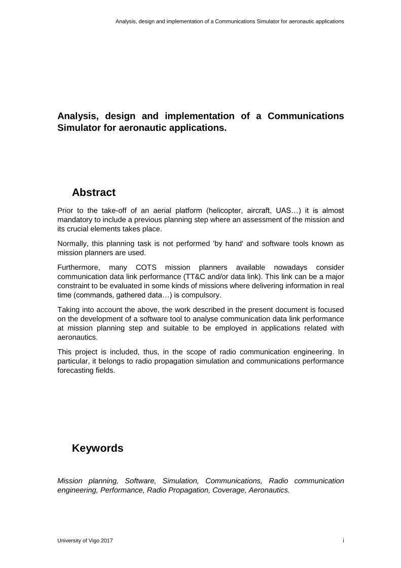
Abstract
Prior to the take-off of an aerial platform (helicopter, aircraft, UAS…) it is almost
mandatory to include a previous planning step where an assessment of the mission and
its crucial elements takes place.
Normally, this planning task is not performed 'by hand' and software tools known as
mission planners are used.
Furthermore, many COTS mission planners available nowadays consider
communication data link performance (TT&C and/or data link). This link can be a major
constraint to be evaluated in some kinds of missions where delivering information in real
time (commands, gathered data…) is compulsory.
Taking into account the above, the work described in the present document is focused
on the development of a software tool to analyse communication data link performance
at mission planning step and suitable to be employed in applications related with
aeronautics.
This project is included, thus, in the scope of radio communication engineering. In
particular, it belongs to radio propagation simulation and communications performance
forecasting fields.
Keywords
Mission planning, Software, Simulation, Communications, Radio communication
engineering, Performance, Radio Propagation, Coverage, Aeronautics.

Analysis, design and implementation of a Communications Simulator for aeronautic applications
University of Vigo 2017 iii
Acknowledgements
A realización deste proxecto supón tamén a última etapa dun período de seis anos
formándome na universidade, seis anos cargados de coñecementos, experiencias e,
sobre todo, persoas que fixeron posible que sexa quen son hoxe e que chegase ata
aquí. Con estas palabras pretendo dar as gracias a todas aquelas persoas que teñen
formado parte da miña vida nestes anos.
En primeiro lugar, gustaríame agradecer á miña familia polo esforzo que supuxo que
leve seis anos estudando na universidade así como polo apoio incondicional na decisión
de adicarme á enxeñaría de Telecomunicacións.
Despois disto, non podo esquecer á xente que estivo aí todo este tempo, e que segue
a estalo a día de hoxe, a familia que se escolle: todos os meus amigues, esa xente que
fixo máis levadeiro o camiño e que me acompañou nel, facendo que os baches doesen
menos e os éxitos fosen máis doces.
Por outro lado, tamén me gustaría dar as gracias a todos os mestres que ó longo destes
anos conseguiron, dun xeito ou doutro, que crecese como persoa e ampliase os meus
coñecementos en ámbitos que van máis aló do puramente académico. Tampouco podo
deixar de lembrarme de todas as persoas que formaron parte da D.AA.T. estes anos,
posto que xunto a eles puiden comprender mellor o funcionamento interno dun centro
universitario (neste caso a EET) e aplicar ditos coñecementos para defender os dereitos
dos alumnos. A súa labor permitiu axudar a moitas persoas no ámbito da Escola, e non
podo máis que desexarlles o mellor ós integrantes actuais e ós que están por vir, porque
estou seguro de que seguirán a facelo.
Ademáis, non podo deixar de lembrar aquí a todas as persoas que forman parte de
Gradiant. Dende o Director da Área de Comunicacións Avanzadas, que me deu a
oportunidade de formar parte do equipo, a todas as persoas que o forman por estar
sempre dispostas a ensinar e a inverter o seu tempo comigo así como a todo o Centro
en xeral por facerme sentir un máis dende o primeiro día.
Xa rematando, gustaríame agradecer ós meus titores neste proxecto (Jorge Munir El-
Malek Vázquez e José Antonio Rodríguez Negro) pola confianza depositada, os
consellos, o apoio e o tempo adicados.
Finalmente, pero non por iso menos importante, gustaríame agradecer á miña parella
por toda a paciencia, comprensión e apoio ó longo destes dous anos.

Analysis, design and implementation of a Communications Simulator for aeronautic applications
University of Vigo 2017 Page | 1
Table of Contents
ABSTRACT ................................................................................................................... I
KEYWORDS ................................................................................................................. I
ACKNOWLEDGEMENTS............................................................................................ III
INDEX OF FIGURES .................................................................................................... 3
INDEX OF TABLES...................................................................................................... 5
INDEX OF EQUATIONS ............................................................................................... 7
ACRONYMS ................................................................................................................. 9
SYMBOLS .................................................................................................................. 11
1. INTRODUCTION .................................................................................................... 13
OVERVIEW ......................................................................................................... 13 OBJECTIVES ....................................................................................................... 13 SCOPE............................................................................................................... 13 DOCUMENT ORGANIZATION ................................................................................. 14
2. ANALYSIS OF THE STATE OF THE ART ............................................................. 15
SOFTWARE SIMULATION TOOLS .......................................................................... 15 2.1.1. Mission Planners ........................................................................................ 15 2.1.2. Radio propagation simulators ..................................................................... 19 2.1.3. All-in-one software tools ............................................................................. 30
RADIO PROPAGATION MODELLING ........................................................................ 32 2.2.1. Initial considerations .................................................................................. 32 2.2.2. Consolidated propagation models .............................................................. 33 2.2.3. Academic review ........................................................................................ 38
DIGITAL TERRAIN MODELS .................................................................................. 40 2.3.1. Initial considerations .................................................................................. 40 2.3.2. Reviewed Digital Terrain Models ................................................................ 40 2.3.3. Complements to Digital Terrain Models ..................................................... 43
INTERFERENCE ANALYSIS ................................................................................... 43 2.4.1. Parametric analysis .................................................................................... 43 2.4.2. Statistical analysis ...................................................................................... 44 2.4.3. Further considerations ............................................................................... 44
ANTENNA RADIATION PATTERNS .......................................................................... 45 WEATHER FORECASTING .................................................................................... 45
2.6.1. Rain attenuation modelling ......................................................................... 45 2.6.2. Sources of meteorological information ....................................................... 46
CONCLUSIONS DRAWN OF THE STATE OF THE ART ................................................ 47
3. DESIGN OF THE APPLICATION ........................................................................... 49
REQUIREMENTS ................................................................................................. 49 3.1.1. Functional requirements ............................................................................. 49 3.1.2. Non-Functional requirements ..................................................................... 50
DECISION MAKING .............................................................................................. 51 3.2.1. Selected propagation model....................................................................... 51
Analysis, design and implementation of a Communications Simulator for aeronautic applications
Page | 2 University of Vigo 2017
3.2.2. Selected Digital Terrain Model ................................................................... 52 3.2.3. Selected modes of operation...................................................................... 52 3.2.4. Selected functionalities .............................................................................. 53 3.2.5. Structure of the simulator ........................................................................... 61
APPROACH TO DESIGN PROCESS ......................................................................... 65 3.3.1. Steps of design process ............................................................................. 65
4. IMPLEMENTATION OF THE PROTOTYPE AND VERIFICATION PROCESS ...... 67
SELECTED IMPLEMENTATION LANGUAGE .............................................................. 67 I/O SUMMARY .................................................................................................... 68
4.2.1. Defined Inputs ............................................................................................ 68 4.2.2. Defined outputs .......................................................................................... 70
IMPLEMENTATION PROCESS ................................................................................ 70 4.3.1. Introduction to implementation process ...................................................... 70 4.3.2. Main window .............................................................................................. 71 4.3.3. Point to Point Mode .................................................................................... 72 4.3.4. Route Mode ............................................................................................... 73 4.3.5. Area mode ................................................................................................. 73 4.3.6. Satellite Mode ............................................................................................ 74 4.3.7. Antenna radiation pattern import window ................................................... 74 4.3.8. Radio Modem Import window ..................................................................... 75 4.3.9. Extra graphs .............................................................................................. 75 4.3.10. Warning auxiliary windows ....................................................................... 75
DEPLOYMENT ANALYSIS ...................................................................................... 75 PERFORMANCE MEASUREMENT ........................................................................... 75 IMPLEMENTATION TESTING AND VERIFICATION ...................................................... 76
5. CONCLUSIONS ..................................................................................................... 79
6. FUTURE LINES OF DEVELOPMENT .................................................................... 81
UPGRADES OVER EXISTING FEATURES ................................................................. 81 NEW FEATURES .................................................................................................. 82
6.2.1. Functional Features ................................................................................... 82 6.2.2. Operational Features ................................................................................. 82
7. REFERENCES ....................................................................................................... 85
ANNEXES .................................................................................................................. 89
ANNEX I: PERFORMANCE MEASUREMENT TESTS RAW DATA .......................... 91
Analysis, design and implementation of a Communications Simulator for aeronautic applications
University of Vigo 2017 Page | 3
Index of Figures
Fig. 1. Evolution of mission planners developed by Boeing along time [4]. .................. 16 Fig. 2. UgCS Mission Planner architecture diagram [9]. .............................................. 18 Fig. 3. Predicted WNYE-DT signal strength contours with color key displayed in Google
Earth [12]. ................................................................................................................... 20 Fig. 4. Point to point path profile generated with SPLAT [12]. ..................................... 21 Fig. 5. Pathloss 5 point to point analysis window [17]. ................................................. 24 Fig. 6. Pathloss 5 multi-location analysis window [17]. ................................................ 25 Fig. 7. PlotPath sample window showing inputs and display of path profile [18]. ......... 26 Fig. 8. Probe4 Graphic User Interface [19]. ................................................................. 27 Fig. 9. OpenGL 3D engine for Terrain-3D [20]. ........................................................... 28 Fig. 10. TIREM flow chart diagram [39]. ...................................................................... 37 Fig. 11. Example of interference parametric analysis. ................................................. 44 Fig. 12. Initial position of the aerial platform antenna. ................................................. 57 Fig. 13. Initial position of the base station antenna. ..................................................... 58 Fig. 14. Three axis rotation matrices. .......................................................................... 58 Fig. 15. Main window layout. ....................................................................................... 62 Fig. 16. Point to Point mode window layout. ................................................................ 63 Fig. 17. Route and Area mode window layout. ............................................................ 63 Fig. 18. Satellite mode window layout. ........................................................................ 64 Fig. 19. Simulator's command line version internals’ structure. ................................... 64 Fig. 20. Incremental implementation procedure flow diagram. .................................... 71 Fig. 21. Simulator’s main window. ............................................................................... 72 Fig. 22. Point to point mode after execution. ............................................................... 72 Fig. 23. Simulator's route mode after execution. ......................................................... 73 Fig. 24. Generated KML file for area mode displayed in Google Earth [69] . ............... 73 Fig. 25. Simulator's satellite mode results display after execution. .............................. 74 Fig. 26. Auxiliary window for importing base station's 3D antenna radiation pattern. ... 74

Analysis, design and implementation of a Communications Simulator for aeronautic applications
University of Vigo 2017 Page | 5
Index of Tables
Table 1. Summary of reviewed propagation simulators. .............................................. 19 Table 2. Summary of reviewed all-in-one tools............................................................ 32 Table 3. Parameter comparison table for some of the different propagation models
analised. ..................................................................................................................... 38 Table 4. Communications Simulator minimum functional requirements. ..................... 50 Table 5. Communications Simulator minimum non-functional requirements. .............. 51 Table 6. Inputs defined for Simulator’s point to point, route and area modes. ............. 69 Table 7. Inputs defined for Simulator's satellite mode. ................................................ 69 Table 8. Outputs definition for Simulator's point to point, route and area modes. ........ 70 Table 9. Outputs definition for Simulator's satellite mode. ........................................... 70 Table 10. Requirements review chart. ......................................................................... 77 Table 11. Performance analysis raw data for simulator’s command line version (one run).
................................................................................................................................... 91 Table 12.Performance analysis raw data for simulator’s GUI version (one run). ......... 91 Table 13. Performance analysis raw data for simulator’s command line version with no
real time rain calculations (Ten runs). ......................................................................... 92 Table 14. Performance analysis raw data for simulator’s command line version with real
time rain calculations (Ten runs). ................................................................................ 93

Analysis, design and implementation of a Communications Simulator for aeronautic applications
University of Vigo 2017 Page | 7
Index of Equations
Eq. 1. Friis Free Space Losses. .................................................................................. 53 Eq. 2. Cross-over distance. ......................................................................................... 53 Eq. 3. Equations for Two-Ray Friis model approximation calculations. ....................... 54 Eq. 4. Equation for Link budget calculations. .............................................................. 54 Eq. 5. Equation for received power calculations. ......................................................... 54 Eq. 6. Noise level calculations. ................................................................................... 54 Eq. 7. SNR estimation equation. ................................................................................. 54 Eq. 8. Check of LoS conditions. .................................................................................. 55 Eq. 9. 1st Fresnel zone radius calculation equation. ................................................... 55 Eq. 10. Doppler shift calculations for static transmitter. ............................................... 55 Eq. 11. Shannon-Hartley channel’s capacity theorem ................................................. 56 Eq. 12. Equation used in Transmission Rate estimation. ............................................ 56 Eq. 13. Transformation of Cartesian coordinates by using rotation matrices. .............. 58

Analysis, design and implementation of a Communications Simulator for aeronautic applications
University of Vigo 2017 Page | 9
Acronyms
3GPP 3rd Generation Partnership Project 3GPP2 3rd Generation Partnership Project 2
AP Aerial Platform API Application Programming Interface ASC ASCII Esri Grid Data
ASTER Advanced Spaceborne Thermal Emission and Reflection Radiometer BS Base Station
COTS Commercial Of-The-Shelf CRC Cyclic Redundancy Check CSV Comma Separated Values DB DataBase
DEM Digital Elevation Model DSM Digital Surface Model DTM Digital Terrain Model ETRS European Terrestrial Reference System
ETRS89 European Terrestrial Reference System 1989 GIS Geographical Information System GUI Graphical User Interface GSM Global System for Mobile communications
H Horizontal HTTP Hypertext Transfer Protocol ITU International Telecommunications Union
ITU-R International Telecommunications Union, Radio communications section ITWOM Irregular Terrain With Obstructions Model JSON JavaScript Object Notation KML Keyhole Markup Language
LHCP Left Handed Circular Polarization LiDAR Light Detection and Ranging or Laser Imaging Detection and Ranging
LoS Line of Sight LTE Long Term Evolution MP Mission Planner
MPS Mission Planning Systems MSL Mean Sea Level NAD North American Datum
NASA North American Space Agency NLoS Non Line of Sight OSM Open Street Map PFPS Portable Flight Planning System PLF Polarization Loss Factor RAM Random Access Memory RF Radio Frequency
RHCP Right handed Circular Polarization SAR Search and Rescue SaaS Software as a Service SDK Software Development Kit SINR Signal to Noise plus Interference Ratio SNR Signal to Noise Ratio SoA State of the Art SOA Service Oriented Architecture
SPLAT RF Signal Propagation, Loss and Terrain SRTM Shuttle Radar Topography Mission TIREM Terrain Integrated Rough Earth Model

Analysis, design and implementation of a Communications Simulator for aeronautic applications
Page | 10 University of Vigo 2017
UAV Unmanned Air Vehicle UHF Ultra High Frequency
USGS United States Geographical Survey UTM Universal Transverse Mercator
V Vertical VHF Very High Frequency VOR VHF Omni Directional Radio Range WCS World Coverage Server WGS World Geodetic System WMS Web Map Service WWS World Wind Server
Analysis, design and implementation of a Communications Simulator for aeronautic applications
University of Vigo 2017 Page | 11
Symbols
𝛂𝐠𝐫𝐨𝐮𝐧𝐝 Elevation angle between the horizontal of the transmitter and an arbitrary path point.
Deg.
𝜶𝒕𝒙−𝒓𝒙 Elevation angle of the receiver as seen by the transmitter under LoS assumption
Deg.
𝐁𝐖 Bandwidth MHz
𝐜 Speed of light m/s
𝑪𝑯𝒄𝒂𝒑 Estimated Channel Capacity Mbps
𝒅 Distance km
𝒅𝒔 Distance to initial path’s point from the nth point km
𝒅𝒆 Distance to final path’s point from the nth point km
𝒅𝒄 Cross-over distance km
𝑫𝒔 Doppler Shift Hz
𝜼 Computation efficiency points/s
𝒇 Frequency MHz
𝐹𝑟𝑐𝑙𝑒𝑎𝑟 Fresnel Clearance %
𝑭𝒓𝒙 Receiver Noise Figure dB
𝑮𝒓𝒙 Receiver gain dB
𝑮𝒕𝒙 Transmitter gain dB
𝒌𝒃𝒐𝒍𝒕𝒛 Boltzmann constant J/K
𝝀 Wavelength m
𝑳𝒆𝒙𝒕𝒓𝒂 Extra losses dB
𝑳𝒇𝒔 Free Space Losses dB
𝑳𝑳𝒊𝒏𝒌 Link budget (losses) dB
𝑳𝒎𝒐𝒅𝒆𝒍 Model losses dB
𝑳𝒓𝒙 Receiver losses dB
𝑳𝒕𝒙 Transmitter losses dB
𝑴 Number of symbols in constellation units
𝑵𝒔 Noise level dBm
𝒑𝒍𝒇 Polarization Loss Factor dB
𝑹𝒙𝒑𝒐𝒘𝒆𝒓 Received power dBm
𝑻𝒙𝒑𝒐𝒘𝒆𝒓 Transmitted power dBm
𝑻𝒙𝒓𝒂𝒕𝒆 Transmission rate Mbps
𝑺𝑵𝑹𝒆𝒔𝒕 Estimated SNR level dBm
𝒗𝒓𝒆𝒍 Relative aerial platform speed m/s

Analysis, design and implementation of a Communications Simulator for aeronautic applications
University of Vigo 2017 Page | 13
1. Introduction
Overview
Nowadays, many commercial available mission planners, used to plan aeronautic
missions in a step prior to take off, take into account communication data link
performance.
The inputs for these kind of software tools are variables like terrain profile in the mission
area, weather forecasts, potential threats or similar ones that can influence in the
success or the failure of the mission if they are not well identified and evaluated.
Taking into account the available data inputs, mission planers can determine the optimal
route according to predefined parameters for the flight and some other constraints to be
taken into account in order to fulfil the mission.
Considering that communication data link performance could be decisive to fulfil a
mission in some cases (such as scenarios where Real Time data acquisition or event
based decision making are mandatory), this project is focused on designing and
developing a software tool to model, forecast and evaluate communication data
link performance along the flight of an aerial platform before its take off considering
different configuration parameters such as flight altitude, flight speed, planned route,
transmission power, antenna’s gain and more.
This configuration parameters can be combined and used as inputs to radio propagation
models that provide information about the radio channel state.
Objectives
The main objectives of this Master’s Thesis are presented below:
The first objective has been to analyse SoA and understand if there were similar
approaches to the topic. Multiple commercial software solutions have been gathered and
analysed as well as research reports and papers related to this topic in order to study
the different elements that needed to be addressed in order to being able to develop a
suitable application.
The second objective, when the initial analysis ended, was focused on establishing
the main functional and technical features of the tool including inputs & outputs as
well as its graphical interface. This implied to go beyond the previous analysis, searching
for information about how things could be done in order to give the desired functionalities
to the developed tool.
At last, the third objective was to implement the simulation tool with its selected
functionalities, making use of the information gathered previously as well as with some
continuous research on solving the issues happened during implementation step.
Scope
The scope of this Master’s Thesis is to design and develop a software tool able to
model communication data link performance in a complex environment, aiding in the
decisions prior to the start of an aerial platform’s mission.

Analysis, design and implementation of a Communications Simulator for aeronautic applications
Page | 14 University of Vigo 2017
This software tool will make use of radio propagation models and terrain elevation data
to obtain information related with datalink performance.
Document organization
In the following paragraphs, the structure of this document will be presented.
After this introductory Introduction, the analysis of the State of the Art of the different
topics involved in this work (software simulation tools, radio propagation modelling…)
can be found in Chapter 2.
Chapter 3 addresses the design process of the application, highlighting some
relevant parts of it. Among them are the requirements imposed to the application and the
decision making process prior to the beginning of the implementation (elements to be
included, structure of the application and so on).
After that, the implementation process is shown in Chapter 4. In addition, the
performed steps in order to test and validate the functionality of the application are
included in this chapter as well.
Chapters 5 and 6 present the Conclusions drawn at the end of the project and the
Future Lines of Development related to the development of the application.
At last, Chapter 7 shows the Bibliography and References employed during this
project.
Annexes:
Annex I: performance measurement tests raw data.
Analysis, design and implementation of a Communications Simulator for aeronautic applications
University of Vigo 2017 Page | 15
2. Analysis of the state of the art
This Chapter focuses on the analysis of several concepts related with the state of the art
of the topic. This analysis has been summarized in the following sections which each
one of them focused in a particular field of interest.
Software Simulation Tools
Being the design, implementation and development of a communications simulator for
aeronautical applications one of the main goals of this project, the first step seems to be
taking a look at what are the existing solutions in the market, what benefits does they
offer and the associated costs of them. Below are the most relevant alternatives that has
been found.
In order to establish a classification, three categories are set.
2.1.1. Mission Planners
The different tools (applications) available in nowadays in the scope of management of
aerial platforms (mainly UAVs or fleets, but its usage may be extended to any other kind
of aeronautic device), whether document management (logs, briefing / debriefing, etc.)
or more oriented to the preparation and / or mission execution belong to this first
subsection.
Portable Flight Planning Software (PFPS)
The Portable Flight Planning Software, or PFPS, [1] is an integrated suite of PC-based
mission planning tools using a common graphical user interface. PFPS is installable on
any Windows 2000 or XP PC. It displays standard digital maps and produces user-
customizable kneeboard cards, combat mission folders, and data transfers to compatible
digital transfer devices. The PFPS software uses an implementation of the client-server
data model to provide a shared view of the mission route to software components. The
PFPS Route Server synchronizes the different PFPS components so that changes made
to the route by one PFPS application are passed to all other components. This allows
the operator to perform multiple operations on the same routes without re-entering data.
The PFPS software suite includes FalconView, Combat Flight Planning Software
(CFPS), Combat Weapon Delivery Software (CWDS), Combat Air Drop Planning
Software (CAPS), and several other software packages built by different software
contractors.
This is a software developed for United States military forces.
Mission Planning Systems (MPS)
The Mission Planning Systems (MPS) program [2] is a collaborative program with the
Army and Navy to leverage technical solutions and business practices for all Department
of Defense (DoD) platforms. It provides automated mission planning tools and support
for fixed and rotary wing aircraft and guided munitions. It will replace two closed
Analysis, design and implementation of a Communications Simulator for aeronautic applications
Page | 16 University of Vigo 2017
architecture legacy mission planning systems (Unix-based MPS (Unix-MPS) and the PC-
based Portable Flight Planning Software (PFPS)), with a single multi-service open
architecture system more commonly referred to as the Joint Mission Planning System
(JMPS). MPS will compress the mission planning cycle by providing an improved
integrated planning environment, reducing the time required to respond to changing
situations and urgent needs such as striking time sensitive/critical targets and conducting
combat search and rescue. MPS, whose development has not ended [3], will deliver
significant benefits to command and control performance by enhancing information
superiority for the warfighter and by providing unique capabilities in support of both
precision engagement and dominant maneuver. Additionally, elements of Mission
Planning Systems will be utilized to continue the development of a Joint Precision Airdrop
System (JPADS) in conjunction with the Army.
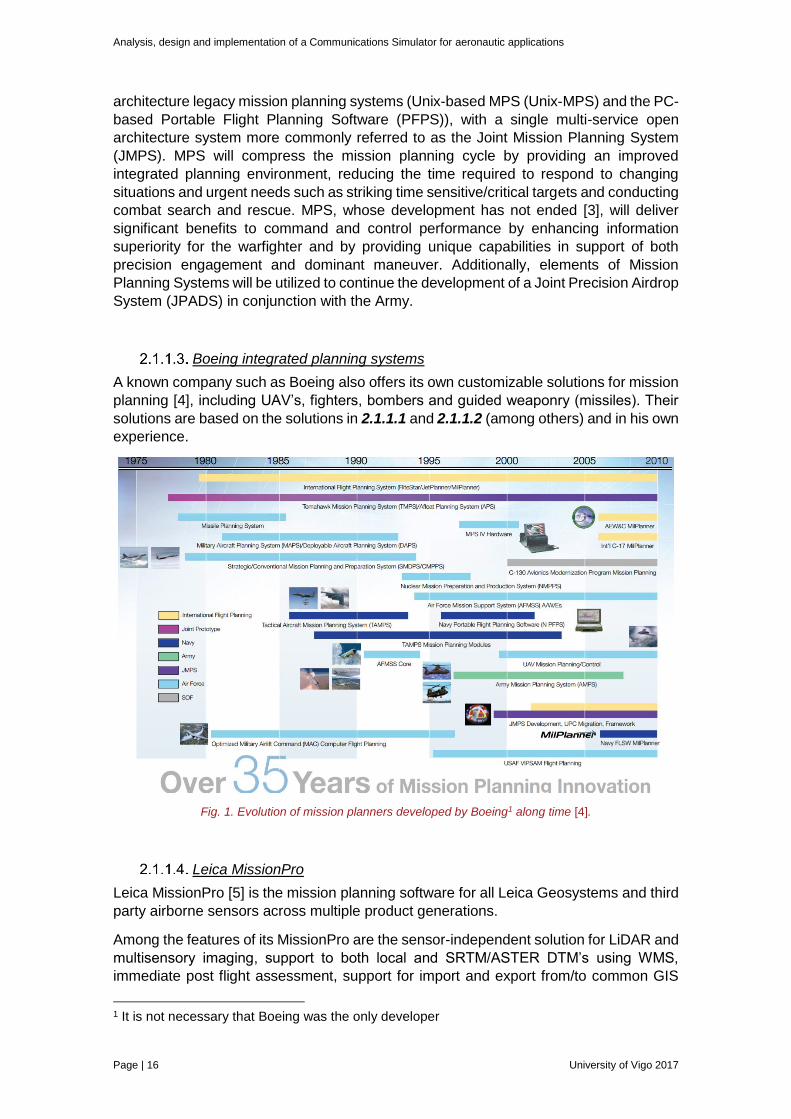
Boeing integrated planning systems
A known company such as Boeing also offers its own customizable solutions for mission
planning [4], including UAV’s, fighters, bombers and guided weaponry (missiles). Their
solutions are based on the solutions in 2.1.1.1 and 2.1.1.2 (among others) and in his own
experience.
Fig. 1. Evolution of mission planners developed by Boeing1 along time [4].
Leica MissionPro
Leica MissionPro [5] is the mission planning software for all Leica Geosystems and third
party airborne sensors across multiple product generations.
Among the features of its MissionPro are the sensor-independent solution for LiDAR and
multisensory imaging, support to both local and SRTM/ASTER DTM’s using WMS,
immediate post flight assessment, support for import and export from/to common GIS
1 It is not necessary that Boeing was the only developer
Analysis, design and implementation of a Communications Simulator for aeronautic applications
University of Vigo 2017 Page | 17
file formats, graphical evaluation and flight comparison with the original plan and the
capability to use a 3D virtual globe view to perform plan analysis.
In addition, it also offers support for project management by providing a scalable
database architecture in SQL.
Leica Geosystems is part of Hexagon [6], a global provider of information technologies
across geospatial and industrial enterprise applications.
SE7EN: Mission Planner
SE7EN: Mission Planner [7] is an interactive touch optimized digital sand table that gives
military and disaster-response mission planners the power to create, plan, and fully
manage missions and logistical routing in a collaborative geospatial environment. It
provides step-by-step walkthroughs or full playbacks and keeps track of altitude for
relative views during mission play through.
It also supports support the WMS Interface Standard, which lets you choose details from
many different geospatial databases to add to your maps, such as temperature, weather
conditions, cloud cover, and others.
This is a special case because it is not a mission planning tool restricted only to
aeronautic applications. Instead of this, it can be used to plan land, air or sea missions
(or any combination of them).
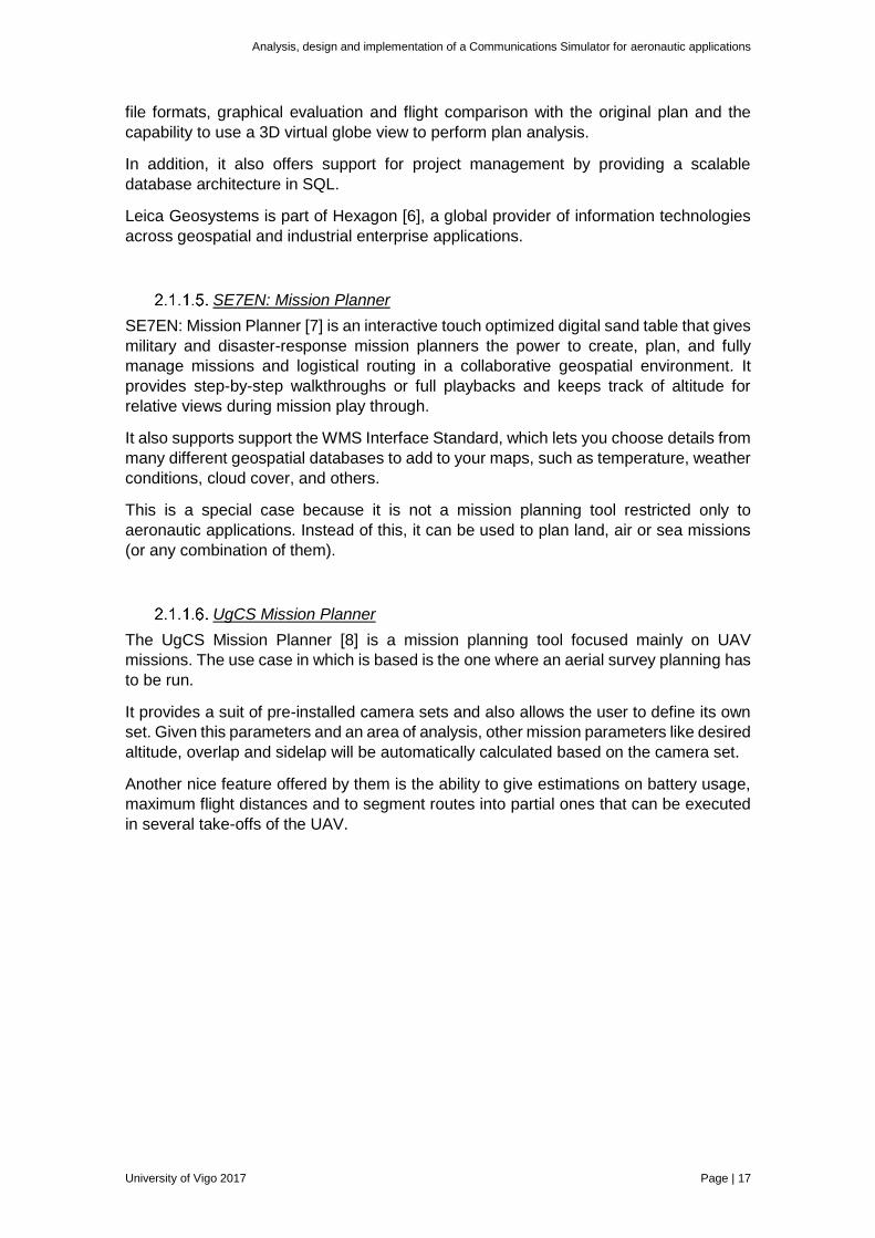
UgCS Mission Planner
The UgCS Mission Planner [8] is a mission planning tool focused mainly on UAV
missions. The use case in which is based is the one where an aerial survey planning has
to be run.
It provides a suit of pre-installed camera sets and also allows the user to define its own
set. Given this parameters and an area of analysis, other mission parameters like desired
altitude, overlap and sidelap will be automatically calculated based on the camera set.
Another nice feature offered by them is the ability to give estimations on battery usage,
maximum flight distances and to segment routes into partial ones that can be executed
in several take-offs of the UAV.
Analysis, design and implementation of a Communications Simulator for aeronautic applications
Page | 18 University of Vigo 2017
Fig. 2. UgCS Mission Planner architecture diagram [9].
It supports the use of DTM’s and in-flight telemetry display including battery level, GPS
signal quality, course and heading, flight speed and more.
In addition to the previous features, an SDK suitable for building custom client
applications (written in C#) is provided.
SkySense BVLOS Planner
The SkySense’s BVLOS Planner [10] is a mission planning tool that will be Open Source
(it seems to be still under development and on its website can only be requested 'early
access').
Analysis, design and implementation of a Communications Simulator for aeronautic applications
University of Vigo 2017 Page | 19
Mission Planner
Mission Planner [11] is a full-featured ground station application for the ArduPilot open
source autopilot project. It is a free, open-source, community-supported application
developed by Michael Oborne for the open-source APM autopilot project.
It also provides a tool for creating automated missions that will run when the ArduPilot is
set to AUTO mode.
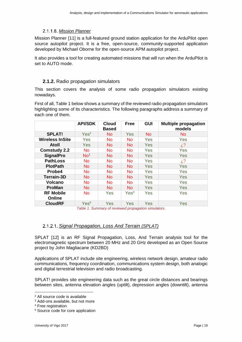
2.1.2. Radio propagation simulators
This section covers the analysis of some radio propagation simulators existing
nowadays.
First of all, Table 1 below shows a summary of the reviewed radio propagation simulators
highlighting some of its characteristics. The following paragraphs address a summary of
each one of them.
API/SDK Cloud Based
Free GUI Multiple propagation models
SPLAT! Yes2 No Yes No No
Wireless InSite Yes No No Yes Yes
Atoll Yes No No Yes ¿?
Comstudy 2.2 No No No Yes Yes
SignalPro No3 No No Yes Yes
PathLoss No No No Yes ¿?
PlotPath No No No Yes Yes
Probe4 No No No Yes Yes
Terrain-3D No No No Yes Yes
Volcano No No No Yes Yes
ProMan No No No Yes Yes
RF Mobile Online
No Yes Yes4 Yes Yes
CloudRF Yes5 Yes Yes Yes Yes Table 1. Summary of reviewed propagation simulators.
Signal Propagation, Loss And Terrain (SPLAT)
SPLAT [12] is an RF Signal Propagation, Loss, And Terrain analysis tool for the electromagnetic spectrum between 20 MHz and 20 GHz developed as an Open Source project by John Magliacane (KD2BD)
Applications of SPLAT include site engineering, wireless network design, amateur radio communications, frequency coordination, communications system design, both analogic and digital terrestrial television and radio broadcasting.
SPLAT! provides site engineering data such as the great circle distances and bearings between sites, antenna elevation angles (uptilt), depression angles (downtilt), antenna
2 All source code is available 3 Add-ons available, but not more 4 Free registration 5 Source code for core application
Analysis, design and implementation of a Communications Simulator for aeronautic applications
Page | 20 University of Vigo 2017
height above mean sea level, antenna height above average terrain, bearings and distances to known obstructions based on USGS and SRTM elevation data, path loss and field strength based on the Longley Rice Irregular Terrain as well as the new Irregular Terrain With Obstructions (ITWOM v3.0) model, and minimum antenna height requirements needed to establish line-of-sight communication paths and Fresnel Zone clearances absent of obstructions due to terrain.
SPLAT produces reports, graphs, and highly detailed and carefully annotated topographic maps depicting line-of-sight paths, path loss, field strength and expected coverage areas of transmitters and repeater systems.
When performing line-of-sight analysis in situations where multiple transmitter or repeater sites are employed, it determines individual and mutual areas of coverage within the network specified.
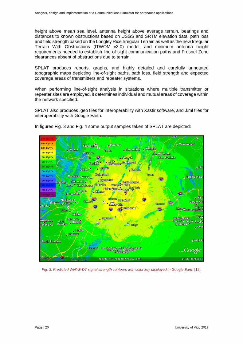
SPLAT also produces .geo files for interoperability with Xastir software, and .kml files for interoperability with Google Earth.
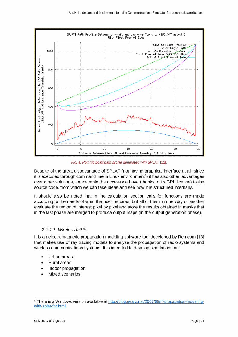
In figures Fig. 3 and Fig. 4 some output samples taken of SPLAT are depicted:
Fig. 3. Predicted WNYE-DT signal strength contours with color key displayed in Google Earth [12].
Analysis, design and implementation of a Communications Simulator for aeronautic applications
University of Vigo 2017 Page | 21
Fig. 4. Point to point path profile generated with SPLAT [12].
Despite of the great disadvantage of SPLAT (not having graphical interface at all, since
it is executed through command line in Linux environment6) it has also other advantages
over other solutions, for example the access we have (thanks to its GPL license) to the
source code, from which we can take ideas and see how it is structured internally.
It should also be noted that in the calculation section calls for functions are made
according to the needs of what the user requires, but all of them in one way or another
evaluate the region of interest pixel by pixel and store the results obtained in masks that
in the last phase are merged to produce output maps (in the output generation phase).
Wireless InSite
It is an electromagnetic propagation modeling software tool developed by Remcom [13]
that makes use of ray tracing models to analyze the propagation of radio systems and
wireless communications systems. It is intended to develop simulations on:
Urban areas.
Rural areas.
Indoor propagation.
Mixed scenarios.
6 There is a Windows version available at http://blog.gearz.net/2007/09/rf-propagation-modeling-with-splat-for.html
Analysis, design and implementation of a Communications Simulator for aeronautic applications
Page | 22 University of Vigo 2017
This tool has an API that allows users to develop custom applications and use Remcom’s
integrated propagation models in it.
For the development of applications that have their own graphical interface and
visualization tools and integrate InSite content, the calculation engine is available as a
library with API in C++.
InSite provides geometric data of cities, terrain, vegetation, soil types and objects that
can be edited and manipulated, as well as import of terrain elevation files, humidity,
objects and his other supported data types.
The application is able to model parameters like received power, path losses, delay
dispersion, electric field (magnitude and phase), estimated BER and C/I ratio, Doppler
Shift…
Among its suggested applications, they were found relevant the analysis of coverage of
base stations, the simulation effects of shadowing and multipath produced by buildings
and/or terrain and the analysis of communications with terrestrial and / or aerial moving
vehicles.
Atoll
Developed by Forsk, Atoll [14] is a Windows tool for the design and optimization of
wireless networks that focuses on 3GPP and 3GPP2 and allows working on multi-
technology networks including small cells and integrated WiFi.
It allows its operators to automate planning and automation processes using SOA-based
scripting (Service Oriented Architectures).
It incorporates its own GIS specifically designed for use in the context of wireless
communications networks and also has support for web map services, GIS and online
maps such as Bing, Google Earth and OSM as well as integration with SOA
architectures.
In addition, it has a C++ SDK that allows the implementation of extra functional modules
such as new propagation models.
Atoll seems to be more focused on the field of telephony networks. Unlike other software
packages, its added value seems to be its very determined scope instead of offering
versatility.
Comstudy 2.2
Developed by RadioSoft, ComStudy [15] is a software tool designed for Microsoft
Windows offering a simplicity level such as to be used by beginners but powerful enough
to be exploited by professionals of radio communication engineering.
Its graphical interface integrates analysis of coverage and location for AM, FM, TV, point-
to-point and point-to-multipoint communications and for terrestrial mobile services.
It allows the measurement of field strength and transmission matrices (cells containing
signal level information) and makes use of its own terrain data.
Analysis, design and implementation of a Communications Simulator for aeronautic applications
University of Vigo 2017 Page | 23
As inputs, it allows to introduce characteristics of transmitter and receiver and known
system losses, select a propagation model and specify size and resolution of the matrix.
SignalPro
Developed by EDX, SignalPro [16] is a graphical RF network planning tool that supports
frequencies in the 30 MHz-100 GHz range and provides indoor, outdoor and mixed
propagation models (though it seems specialized in urban models) both standard and
proprietary.
Its functionality can be expanded through a series of official add-ons but it does not have
an API to develop on it.
Over propagation models can be adjusted to higher environmental and reliability
parameters as well as adding trees, buildings and other obstacles.
Among its capabilities are to present a number of parameters’ estimations on interactive
2D and 3D maps. Some of them are listed below:
Line of Sight area.
Channel losses.
Field strength.
Received power.
Estimated BER.
Required antenna height to have LOS conditions.
C / (I + N) ratio.
Link availability percentage.
Delay dispersion.
PathLoss
Developed by Contract Telecommunication Engineering, PathLoss [17] is a graphical
software tool that performs coverage analysis and communication data link performance
in the field of radio wave propagation. The variables considered by the software are listed
below:
Rain models.
Fresnel Zone clearance.
Interferences.
Terrain elevation profile.
Atmospheric absorption.
Multipath.
Diffraction losses.
Buildings profiles and heights.
Terrain usage.
Provides support for exporting data in several formats that are compatible with Google
Earth, MapInfo and ERSI and generates the following types of outputs:
Thematic maps in 2D and 3D (customizable in terms of colour, legend and
information shown).
Graphics.
Analysis, design and implementation of a Communications Simulator for aeronautic applications
Page | 24 University of Vigo 2017
Written reports.
CSV files.
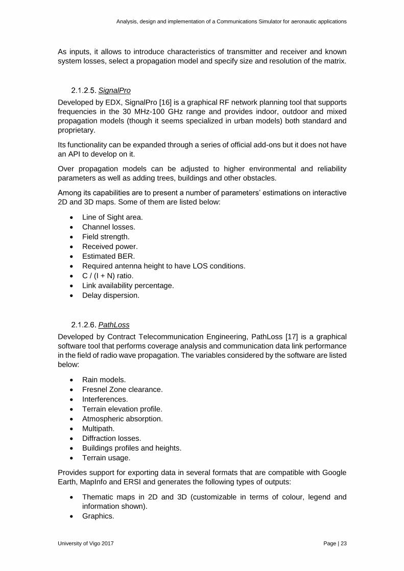
It seems to be one of the most complete tools and its last release, dated 2015, suggest
a relatively continuous support and maintenance. However, it seems that in this case the
propagation model is fixed and cannot be selected among several ones as in previous
cases, but there is no detailed information about that
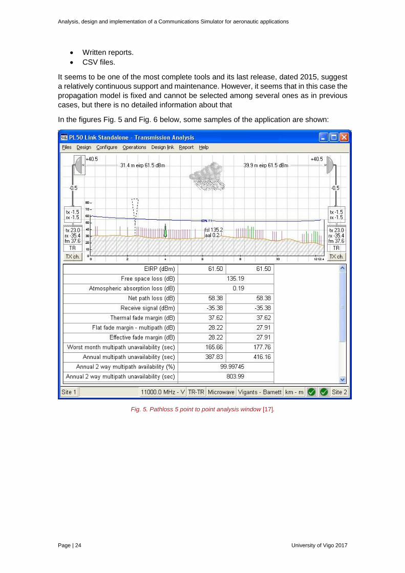
In the figures Fig. 5 and Fig. 6 below, some samples of the application are shown:
Fig. 5. Pathloss 5 point to point analysis window [17].
Analysis, design and implementation of a Communications Simulator for aeronautic applications
University of Vigo 2017 Page | 25
Fig. 6. Pathloss 5 multi-location analysis window [17].
PlotPath
Developed by V-Soft Communications, PlotPath [18] is presented as a software tool for
analysis of radio paths considering terrain elevation data from various sources (housed
in its own database) and displaying the results in 2D graphics and text outputs.
The frequencies available to be studied range from 22 MHz to 35 GHz and it also
considers the effects of Earth’s curvature and Fresnel Zones.
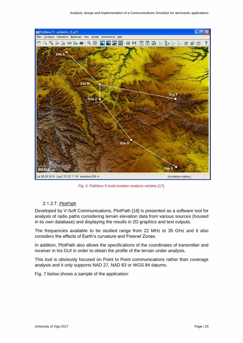
In addition, PlotPath also allows the specifications of the coordinates of transmitter and
receiver in his GUI in order to obtain the profile of the terrain under analysis.
This tool is obviously focused on Point to Point communications rather than coverage
analysis and it only supports NAD 27, NAD 83 or WGS 84 datums.
Fig. 7 below shows a sample of the application:
Analysis, design and implementation of a Communications Simulator for aeronautic applications
Page | 26 University of Vigo 2017
Fig. 7. PlotPath sample window showing inputs and display of path profile [18].
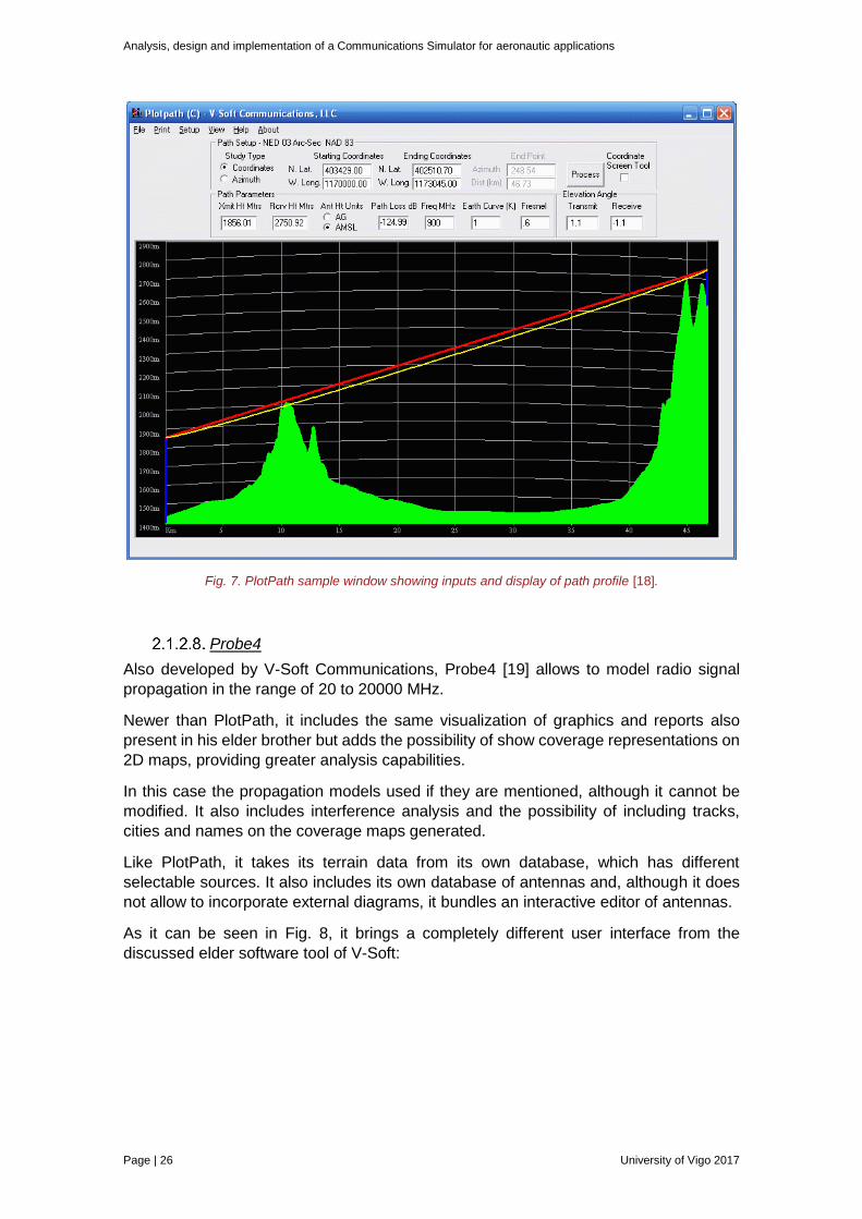
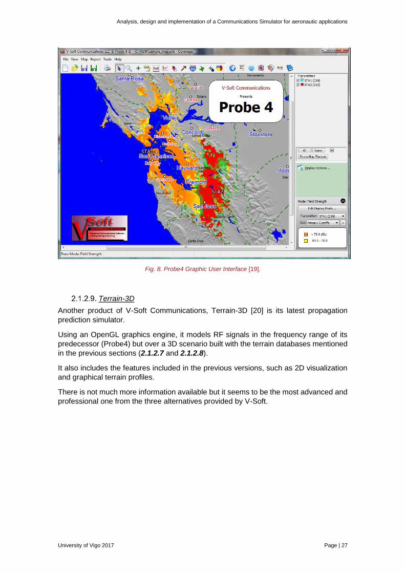
Probe4
Also developed by V-Soft Communications, Probe4 [19] allows to model radio signal
propagation in the range of 20 to 20000 MHz.
Newer than PlotPath, it includes the same visualization of graphics and reports also
present in his elder brother but adds the possibility of show coverage representations on
2D maps, providing greater analysis capabilities.
In this case the propagation models used if they are mentioned, although it cannot be
modified. It also includes interference analysis and the possibility of including tracks,
cities and names on the coverage maps generated.
Like PlotPath, it takes its terrain data from its own database, which has different
selectable sources. It also includes its own database of antennas and, although it does
not allow to incorporate external diagrams, it bundles an interactive editor of antennas.
As it can be seen in Fig. 8, it brings a completely different user interface from the
discussed elder software tool of V-Soft:
Analysis, design and implementation of a Communications Simulator for aeronautic applications
University of Vigo 2017 Page | 27
Fig. 8. Probe4 Graphic User Interface [19].
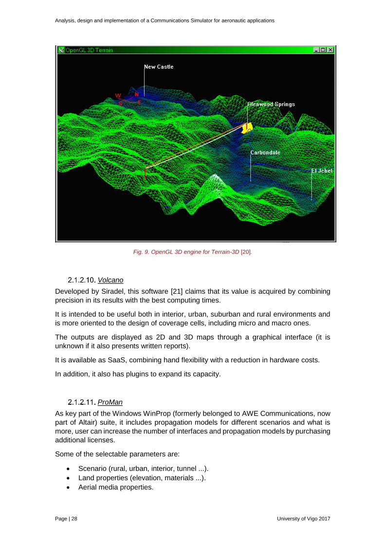
Terrain-3D
Another product of V-Soft Communications, Terrain-3D [20] is its latest propagation
prediction simulator.
Using an OpenGL graphics engine, it models RF signals in the frequency range of its
predecessor (Probe4) but over a 3D scenario built with the terrain databases mentioned
in the previous sections (2.1.2.7 and 2.1.2.8).
It also includes the features included in the previous versions, such as 2D visualization
and graphical terrain profiles.
There is not much more information available but it seems to be the most advanced and
professional one from the three alternatives provided by V-Soft.
Analysis, design and implementation of a Communications Simulator for aeronautic applications
Page | 28 University of Vigo 2017
Fig. 9. OpenGL 3D engine for Terrain-3D [20].
Volcano
Developed by Siradel, this software [21] claims that its value is acquired by combining
precision in its results with the best computing times.
It is intended to be useful both in interior, urban, suburban and rural environments and
is more oriented to the design of coverage cells, including micro and macro ones.
The outputs are displayed as 2D and 3D maps through a graphical interface (it is
unknown if it also presents written reports).
It is available as SaaS, combining hand flexibility with a reduction in hardware costs.
In addition, it also has plugins to expand its capacity.
ProMan
As key part of the Windows WinProp (formerly belonged to AWE Communications, now
part of Altair) suite, it includes propagation models for different scenarios and what is
more, user can increase the number of interfaces and propagation models by purchasing
additional licenses.
Some of the selectable parameters are:
Scenario (rural, urban, interior, tunnel ...).
Land properties (elevation, materials ...).
Aerial media properties.
Analysis, design and implementation of a Communications Simulator for aeronautic applications
University of Vigo 2017 Page | 29
Area of simulation.
Propagation model.
Desired results (from a list).
Transmitter and receiver parameters (antennas’ height, cables’ losses, gains,
antennas’ radiation patterns).
The results are presented by using 2D and 3D maps as well as with written reports and
all the operations can be handled through its built in GUI.
This interface also allows the user to add:
Masks and filters on specific areas.
Evaluation along user-defined paths.
Differences between predictions and measurement results.
Extra layers with data drawn by the user.
And another nice feature available is the capability of exporting maps to other formats
(Google Earth’s .kml, for example).
Its functionality can be extended with other modules of the suite (such as AMan, for
design of antenna radiation patterns) and through a serie of modules that increase the
available propagation models and the networks’ types available to be designed.
RF Mobile Online
This tool, developed by Roger Coudé [22] offers the integration of RF propagation
modelling software with a web platform (it runs as a free tool under previous registration).
It is limited to studies on amateur radio frequency bands and takes into account data of:
Tx power.
Transmitter line losses.
Gain, type, azimuth and height of transmitter antenna.
Transmitter and receiver location.
Elevation data of path between transmitter and receiver.
Gain, type, azimuth and height of transmitter antenna.
Receiver’s sensitivity.
Percentage of time in which the signal must be above a certain threshold.
It makes combined use of three propagation models to estimate the results of analysis.
Other information:
Multiplatform (runs from browser).
Simplified data entry.
Availability of the latest terrain data.
Multithread (two threads per user).
Download generated data to local environment.
Performed studies are saved on its server.
Analysis, design and implementation of a Communications Simulator for aeronautic applications
Page | 30 University of Vigo 2017
CloudRF
This propagation simulation software [23] is based on SPLAT [12] implementation, which
has been included along with more parameters, more propagation models and multi-
threading capabilities.
Like RF Mobile Online, it is intended to be used as a web service, although with fewer
restrictions than this one.
Given its Open Source approach, access to the complete code of the application is
provided. It can be downloaded from git and has to be considered that is designed to be
deployed in a Linux environment. Among the considered data it can be highlighted:
High resolution 3D terrain data available.
3D antenna radiation patterns available.
Consideration of atmospheric and environmental variables.
Many deterministic and empirical models of propagation available.
Other relevant data:
500 km radius of maximum analysis.
Multi-link analysis.
Development API.
Export data to KML, KMZ, SHP and GTIFF.
Global coverage.
2.1.3. All-in-one software tools
The scope of this section is to analyse the existing all-in-one solutions which cover both
mission planning and communication data link performance simulation.
Systems ToolKit (STK)
Developed by AGI, STK [24] is a free simulation software that offers the possibility of
modelling a huge amount of parameters related to both manned and unmanned aircraft
missions. Its most remarkable features include:
Scope and performance of sensors.
Flight conditions.
Characterization of the interaction of multiple aircrafts.
Payload modelling.
Security Validation in Mission Parameters.
Intercommunication between Earth’s base stations and satellites.
Despite the fact that in order to enhance tool’s performance with a more powerful
functionality in the field of communication data link performance simulations it is
advisable to use one of its official plugins (all available through purchase), the
'Communications' plugin [25].
Through this plugin transmitters, receivers (which can be integrated into aircraft models,
ships, vehicles ...) and a wide variety of atmospheric models and terrain can be modelled,
allowing a complete link analysis and availability estimation.
Analysis, design and implementation of a Communications Simulator for aeronautic applications
University of Vigo 2017 Page | 31
STK-Comm takes into account parameters selectable by the user as:
Propagation model (urban and non-urban).
Rain model.
Absorption model.
Multi-beam modelling.
Interference analysis.
Antenna pattern (allows the use of user-imported ones).
Pre-reception and pre-demodulation gains.
Post-transmission gain.
Modulation scheme used.
System noise temperature.
Since the free ‘base’’ version, the obtained results are displayed in 2D or 3D maps in the
application’s own GUI along with the digital terrain models available in its database.
AeroTrackCOM
Developed by Integrasys, it [26] is a commercial simulation software oriented to both
military and civilian applications that allows to configure an UAV prior to a mission paying
attention in its capacity, the communication data link performance and link budget during
its course.
The application models:
Satellite links.
Sensor equipment, satellites and terrestrial infrastructures.
Allows the importation of radiation patterns of antennas.
Interferences.
Influence of meteorology.
There is not much more information regarding this simulator.
Common Open Mission Management Command and Control
(ICOMC2)
Developed by Insitu, ICOMC2 is a software tool [27] that allows to control multiple UAVs
with a single base station and a single operator.
Through its 'RF Link Analysis' Plugin [28], the capability off taking into account variations
of the terrain as well as certain atmospheric conditions (and its effect over
communications) to be able to know in advance the conditions of mission and to
anticipate to the potential problems is provided.
There is not much more information available about this software.
Analysis, design and implementation of a Communications Simulator for aeronautic applications
Page | 32 University of Vigo 2017
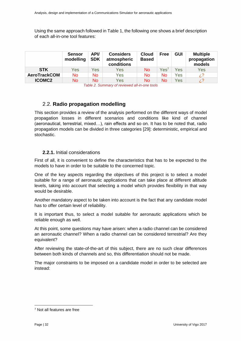
Using the same approach followed in Table 1, the following one shows a brief description
of each all-in-one tool features:
Sensor modelling
API/SDK
Considers atmospheric conditions
Cloud Based
Free GUI Multiple propagation
models
STK Yes Yes Yes No Yes7 Yes Yes
AeroTrackCOM No No Yes No No Yes ¿?
ICOMC2 No No Yes No No Yes ¿? Table 2. Summary of reviewed all-in-one tools
Radio propagation modelling
This section provides a review of the analysis performed on the different ways of model
propagation losses in different scenarios and conditions like kind of channel
(aeronautical, terrestrial, mixed…), rain effects and so on. It has to be noted that, radio
propagation models can be divided in three categories [29]: deterministic, empirical and
stochastic.
2.2.1. Initial considerations
First of all, it is convenient to define the characteristics that has to be expected to the
models to have in order to be suitable to the concerned topic.
One of the key aspects regarding the objectives of this project is to select a model
suitable for a range of aeronautic applications that can take place at different altitude
levels, taking into account that selecting a model which provides flexibility in that way
would be desirable.
Another mandatory aspect to be taken into account is the fact that any candidate model
has to offer certain level of reliability.
It is important thus, to select a model suitable for aeronautic applications which be
reliable enough as well.
At this point, some questions may have arisen: when a radio channel can be considered
an aeronautic channel? When a radio channel can be considered terrestrial? Are they
equivalent?
After reviewing the state-of-the-art of this subject, there are no such clear differences
between both kinds of channels and so, this differentiation should not be made.
The major constraints to be imposed on a candidate model in order to be selected are
instead:
7 Not all features are free
Analysis, design and implementation of a Communications Simulator for aeronautic applications
University of Vigo 2017 Page | 33
Altitude range for which it has been tested / intended
This is important because it is the true fact that will determinate if a model is suitable or
not for airborne applications.
If a model claims to be adequate for a certain altitude, then is reasonable to assume that
all signal impairments that can happen within this altitude range are taken into account
in some way.
Frequency range for which it has been tested / intended
That is another relevant aspect, because of the need to cover a wide spectrum of
possible applications without having knowledge a priori of its operational frequencies.
As broader the frequency range that has been considered within a model as good for
developing a simulator which covers a wide number of use cases will be.
Source of the model (ITU, National Governments, private corporations…)
The owner of the model, or maybe the organization behind its development, is important
because of its relationship with reliability.
For example, a model published in an ITU Recommendation is intended to be reliable
enough to be used while another found in an internet personal blog shall not offer the
same confidence level.
Implementation ease
As has been set in the introduction of the objectives of this project (1.2), one of them is
to design and develop the simulation tool with limited time for do it, so a trade-off between
reliability/accuracy and implementation ease must be considered.
2.2.2. Consolidated propagation models
This subsection addresses both those models produced by International Organizations
(like ITU) and those that are widely used worldwide.
International Telecommunication Union
Recommendation ITU-R P.2001-2
This Recommendation [30], published in July 2015, provides a general purpose semi-
empirical8 propagation model with the following characteristics:
Frequency range of 30 to 50000 MHz.
Distances from 39 to at least 1000 km.
Valid for model basic transmission losses not exceeded in any percentage of time
of an average year (from 0.001 to 99.999 %).
8 Since it combines measurements data with stochastics 9 There is no lower limit, but for smaller distances the clutter effect (buildings, trees, etc.) tend to dominate, unless the antennas are at enough height to ensure an unobstructed path.
Analysis, design and implementation of a Communications Simulator for aeronautic applications
Page | 34 University of Vigo 2017
The height of the antennas cannot be zero, but this method is intended to be
reliable for heights up to 8000 meters above sea level.
From the range of parameters that can be taken into account while modelling radio
channel propagation losses, this Recommendation considers:
Terrain elevation profile.
Link frequency.
Polarization of the antennas.
Transmitter position.
Receiver position.
Antenna’s height.
Percentage of the average for what the calculated transmission losses shall not
be exceeded.
Gains of transmitter and receiver antennas.
It also uses values and constants (conductivity, rainfall parameters, etc.) recommended
by the ITU that can be easily customized if data of the area to be evaluated are available.
Some of these conditions and parameters considered in this model of propagation are:
Weather conditions derived from models provided by the ITU.
Refractivity of the first km of atmosphere.
Refractivity in the first 65 meters of atmosphere.
Rainfall parameters.
Geometry of Earth's effective radius.
Radio horizon boundary parameters.
Factor of 'plain' of the road followed by lightning.
Tropospheric scatter.
Gaseous absorption.
Basic transmission losses in free space.
Diffraction losses produced by knife edge obstacles.
The proposed method is decomposed into 4 sub-models of which each one takes into
account different sets of propagation mechanisms. These sub-models can be combined
to present the final result of basic transmission losses (taking into account some
particular statistics of each sub-model).
Recommendation ITU-R p.2041-0
This Recommendation [31] provides an empirical model to obtain the total attenuation
on a link between an aerial platform and the surface of the Earth (or between an aerial
platform and space).
It makes multiple references to the other ITU-R Recommendations which are
complementary used for its calculations, and it takes into account the following
phenomena:
Attenuation due to rain with a fixed probability.
Gas attenuation.
Attenuation due to clouds.
Fading due to tropospheric scintillation.
These prediction methods can be used to predict the worst case or average link
availability for any applicable elevation profile and elevation angle.
Analysis, design and implementation of a Communications Simulator for aeronautic applications
University of Vigo 2017 Page | 35
Recommendation ITU-R P.528-3
This empirical propagation model provided by ITU [32] is valid for studying the
propagation of the aeronautical mobile and aeronautical radio navigation services in the
VHF, UHF and centimetre (125-15500 MHz) bands.
It contains a method based data interpolation from a series of curves to obtain the basic
transmission losses in ground-air, ground-satellite, air-air, air-satellite and satellite-
satellite links.
The data used are the distance between antennas, their heights above mean sea level,
frequency and percentage of time.
It also allows, with a series of higher data (transmitted power, transmitting antenna gain
and receiving antenna gain) to obtain the expected protection ratio or the desired /
interfering signal ratio exceeded in the receiver 95% of the time.
To perform these calculations it assumes a flat Earth model, with a coefficient of the
earth's fictive radius K of 4/3; it also uses constants for medium terrain, horizontal
polarization, isotropic antennas, and long-term power fade statistics in a temperate
continental climate.
The values of these curves sums the attenuation due to the atmospheric absorption to
the attenuation corresponding to the losses of propagation in free space.
In the area 'near' the radio electric horizon, they are obtained by calculating the values
of the transmission loss according to the laws of geometric optics, in order to take into
account the interference between the direct ray and a reflected ray at the surface of the
Earth .
The formula used to calculate short-term fading includes field reflection and tropospheric
propagation over multiple paths.
The algorithms used to generate the curves the model provides are presented in [33].
There, the so called IF77 propagation model is described for the prediction of basic
transmission losses.
The validity of this method is restricted to the range of 0.1-20 GHz for antennas of more
than half a meter and in scenarios in which the radio horizon has a lower elevation than
the highest antenna.
It is a similar model to the Longley-Rice propagation model (implemented by many
propagation simulation software tools described in 2.1.2) especially designed for
obtaining attenuation / distance curves calculated for Line of Sight (LoS), diffraction and
scatter, which are combined in transition regions. The model includes tolerance for the
incorporation of:
Mean curvature of the rays.
Horizon Effects.
Long term power fading.
Radiation pattern of the antenna (single elevation) in each terminal.
Multipath by surface reflections.
Tropospheric multipath.
Atmospheric absorption.
Ionospheric scintillation.
Rain attenuation.
Analysis, design and implementation of a Communications Simulator for aeronautic applications
Page | 36 University of Vigo 2017
State of the sea.
Divergence Factors.
Very high antennas.
Recommendation ITU-R P.525-2
This Recommendation [34] takes provides formulae for the computing of Free Space
Losses without considering any other phenomenon (like diffraction, rain attenuation,
scattering, multipath ...).
Recommendation ITU-R P.618-12
Taking into consideration the possibility of the aerial platform to communicate with the
space through satellite link, this Recommendation [35] has also been reviewed. It
includes propagation data and prediction methods necessary for the design of Earth-
Space telecommunications links and considers:
Attenuation of atmospheric gases.
Attenuation by clouds and rain.
Loss for 'Beam Spreading'.
Tropospheric scintillation and multipath.
Faraday rotation.
Group Delay.
Ionospheric absorption.
Ionospheric scintillation.
In addition, in Recommendations ITU-R P.681-9 [36] and ITU-R P.682-3 [37] provide
propagation data which may be useful to model Earth-Space mobile telecommunication
systems for land and aeronautical links respectively.
Other widely used models
Irregular Terrain Model
This semi-empirical model [38], also known as Longley-Rice propagation model, is a
widely used propagation losses model in the range of 20-20000 MHz.
It has two modes, the area prediction mode and the point-to-point mode. In the first one,
it uses empirical medians of the terrain profile conditions while in the point-to-point case
it employs terrain data directly.
In the case of LoS trajectories, the attenuation is calculated based on the two-ray theory
and an extrapolated diffraction attenuation value.
It is intended for use in the following conditions (from the original 1968 publication):
Frequency: 20-20000 MHz (in the original publication this range is extended from
20-40000 MHz but many of the software packages that incorporate it fall within
this range).
Antenna height: 0.5-3000 m.
Distance: 1-2000 km.
Surface refractivity: 250-400 N-units.
It takes into account models such as multiple knife-edge and rounded edge diffraction
as well as atmospheric attenuation, tropospheric propagation modes, terrain data,
Analysis, design and implementation of a Communications Simulator for aeronautic applications
University of Vigo 2017 Page | 37
antenna polarization, climate and atmospheric stratification and many more, with most
of them based on experimental measurements.
Terrain Integrated Rough Earth Model (TIREM)
After having found an official US DoD paper [39] detailing the procedures and model
under which TIREM is developed its way of operating can be guessed. It is important to
say that this is the de facto standard for the US federal government and its army in the
field of electromagnetic propagation study and is also used in civil applications like STK
[40].
After performing an initial analysis of the document, it seems that all the equations, data
and elements necessary for the development and implementation of this model are
present, as well as a series of criteria and guides for their application in function of the
obtained results in certain predetermined calculations (what phenomena to take into
account for model losses as a function of LoS / NLoS conditions, frequency ...).
However, more exhaustive review has revealed that certain data come from external
sources that are classified.
Several similarities have been found between this model and others from ITU, but not so
many as to affirm that the results produced would be the same.
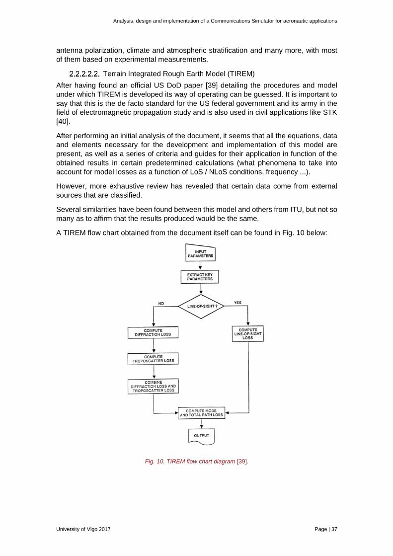
A TIREM flow chart obtained from the document itself can be found in Fig. 10 below:
Fig. 10. TIREM flow chart diagram [39].
Analysis, design and implementation of a Communications Simulator for aeronautic applications
Page | 38 University of Vigo 2017
TIREM model takes into account the following propagation effects:
Free Space Losses.
Reflection.
Propagation by surface wave.
Diffraction.
Propagation by tropospheric scattering.
Atmospheric absorption.
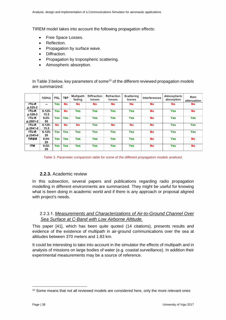
In Table 3 below, key parameters of some10 of the different reviewed propagation models
are summarized:
Table 3. Parameter comparison table for some of the different propagation models analised.
2.2.3. Academic review
In this subsection, several papers and publications regarding radio propagation
modelling in different environments are summarized. They might be useful for knowing
what is been doing in academic world and if there is any approach or proposal aligned
with project's needs.
Measurements and Characterizations of Air-to-Ground Channel Over
Sea Surface at C-Band with Low Airborne Altitude.
This paper [41], which has been quite quoted (14 citations), presents results and
evidence of the existence of multipath in air-ground communications over the sea at
altitudes between 370 meters and 1.83 km.
It could be interesting to take into account in the simulator the effects of multipath and in
analysis of missions on large bodies of water (e.g. coastal surveillance). In addition their
experimental measurements may be a source of reference.
10 Some means that not all reviewed models are considered here, only the more relevant ones
Analysis, design and implementation of a Communications Simulator for aeronautic applications
University of Vigo 2017 Page | 39
Channel models for aeronautical and low elevation radio links
In this document [42], despite being a bit outdated ( it does not take into account the ITU-
R recommendations p.2001-2 and ITU-R p.528-3 as updated propagation models)
shows the existent problems in modelling air attenuation and the rain attenuation
following the existing Recommendations.
It also mentions methods (some developed by ONERA) for the prediction of these
phenomena, as well as scintillation and multipath.
Modelling air-to-ground path loss for low altitude platforms in urban
environments
This paper [43] develops a simulation scenario of radio links in urban areas, describing
the phenomena and parameters to consider when estimating propagation losses in
environments like this.
It bases its data on randomly generated cities using Matlab for geometry and external
data for the different materials that would form the buildings (concrete, crystal ...).
The results’ validation is performed by comparison with results obtained by Wireless
InSite [13] software, with apparently very satisfactory results.
The UAV Low Elevation Propagation Channel in Urban Areas:
Statistical Analysis and Time-Series Generator
This paper [44] show the approach, beginning and initial results [45] of a propagation
measurement campaign in urban environments intended to obtain useful data for their
use in electromagnetic propagation modelling systems.
Aeronautical channel modelling at VHF-band
In the articles found in [46] and [47], different scenarios are presented, or rather different
stages of the same scenario, in which an aircraft is found throughout a mission (flight,
landing, taxi…)
In addition to this, they also characterize some of the phenomena that must be taken into
account or that are dominant in relation to degradations in signal propagation.
All this is focused from a rather statistical point of view that does not take into account
the geometry of each possible realization of the scenarios considered, but is based on
mathematical models, from which link quality parameters like BER can be obtained.
Analysis, design and implementation of a Communications Simulator for aeronautic applications
Page | 40 University of Vigo 2017
Digital Terrain Models
This section covers the different digital terrain elevation models evaluated for being used
in the simulator, the meaning of some if its parameters and characteristics and some
criteria to evaluate them and select the most suitable for the application.
2.3.1. Initial considerations
In order to select an appropriate Digital Terrain Model, is important to pay attention to certain elements that could result being highly troublesome in the next steps of this project (particularly during software implementation). First of all, the selected Digital Terrain Model has to be accessible via http connection or some similar protocol. The main reason supporting this is that there is a limited amount of time to spend in developing the simulator, and by obtaining data via the internet relief us from having to develop a database to store the selected DTM. Moreover, this web connection must support programmatic queries instead of selecting the desired data from a graphical web interface. This will allow the simulator to load the desired DTM without requesting the operator to previously visit a webpage and download the desired data (use of the DTM become transparent to end user). Last but not least, another key aspect which has to be considered to select a proper DTM
is the model's resolution11. Even though radio propagation should not fluctuate much in
few meters, the presence of obstructions surely will affect in a significant way to
communications performance. Therefore, getting better model's resolution will result in
better characterized communication data link performance.
2.3.2. Reviewed Digital Terrain Models
FalconView
FalconView [48] is a Microsoft Windows based mapping application (used by US military)
that displays various types of maps and geographically referenced overlays. Many map
types are supported, but the primary ones of interest to most users are aeronautical
charts, satellite images, and elevation maps. FalconView also supports a large number
of overlay types that can be displayed and printed over any map background. The current
overlay set is oriented toward mission planning and includes many overlays targeted
toward aviators and aviation support personnel as well as overlays of interest to ground
and maritime operators. Additionally, FalconView is used as an on board moving-map
display on several aeronautic platforms. FalconView is an integral part of the Portable
Flight Planning Software (PFPS), and various FalconView components are also being
adapted to the new Joint Mission Planning System (JMPS) environment.
Nevertheless, this is a proprietary software that is not available to be used neither by
students nor companies as it is restricted to U.S. Government and Military.
11 Understand resolution as the capability of distinguishing between many adjacent geographical shapes (mountains, hills, gorges...).
Analysis, design and implementation of a Communications Simulator for aeronautic applications
University of Vigo 2017 Page | 41
NASA WorldWindServer
Free server provided by NASA [49] that has different resources available for download
through queries to the server and that presents / displays integration with many
languages / platforms like Java, Android, Matlab and many more. The maps and
resolutions available for DTMs are the following:
SRTM30 with Bathymetry12 (900m) merged with global ASTER (30m)
Date: --
Coverage: global
Resolution: mixed (900, 30 m)
USGS NED 30m
Date: 2001 (initial, then updates)
Coverage: mainland USA, Alaska, Hawaii and Puerto Rico
Resolution: 30 m
ScankortElevationsDenmarkDSM
Date: 2009
Coverage: Denmark
Resolution: -
ScankortElevationsDenmarkDTM
Date: 2009
Coverage: Denmark
Resolution: 1.6 m / px
Aster_30m
Date: 2000 - present day
Coverage: 83 degrees north ~ 83 degrees south
Resolution: 30 m
SRTM30 with Bathymetry (900m) merged with global ASTER (30m) and
USGS NED (10m)
Date:--
Coverage: global
Resolution: mixed (900, 30, 10 m)13
SRTM30 with Bathymetry (900m) merged SRTM3 V4.1 (90m) and USGS
NED (10m)
Date: --
Coverage: global
Resolution: mixed (900, 90, 10 m)
SRTM30 with Bathymetry (900m) merged SRTM3 V4.1 (90m) and USGS
NED (30m)
Date: --
12 Bathymetry: measurements on water masses depth. 13 ‘Mixed’ resolution means that model’s resolution vary for different locations. For example, a global DTM with 900 m resolution can has 90 m resolution in Spain if the Government promotes a measurement campaign and then gives the obtained results to NASA.
Analysis, design and implementation of a Communications Simulator for aeronautic applications
Page | 42 University of Vigo 2017
Coverage: global
Resolution: mixed (900, 90, 30 m)
SRTM3 V4.1
Date: 2000 (update 2008) - best version available
Coverage: global
Resolution: 90 m
SRTM30 Plus
Date: 2000 (updates until 2014)
Coverage: global
Resolution: 900 m
USGS NED 10m
Date: 2001 (initial, then updates)
Coverage: mainland USA, Alaska, Hawaii and Puerto Rico
Resolution: 10 m
Google Maps API
This alternative [50] is attractive because of the large amount of data that Google handles
and its integration with Google Maps via API.
Its resolution is updated frequently and today is over 30 meters in the worst case. The
main drawback of Google Maps API is the limitation in number of queries to the database
for free development plan, beyond which it is necessary to request a payment plan.
Maps provided by Spanish ‘Instituto Geográfico Nacional’
Through its web portal [51] maps of the whole Spanish territory with resolutions of 200,
25 and 5 meters can be obtained.
The biggest problem is that because of how they are structured, their method of
downloading via web portal instead of server and their data format does not fit the
preliminary requirements imposed.
However, it is possible to obtain elevation data through requests to its WCS server [52].
The maximum resolution of these models is 25 meters, with coverage throughout the
national territory (including the Canary Islands). It allows specifying the coordinates of
the area to be obtained, the sampling period and the type of file to be obtained (.asc or
.gtiff).
Data are available in both UTM coordinates as latitude and longitude, using the ETRS89
datum14.
14 Which is compatible with WGS-84 world datum.
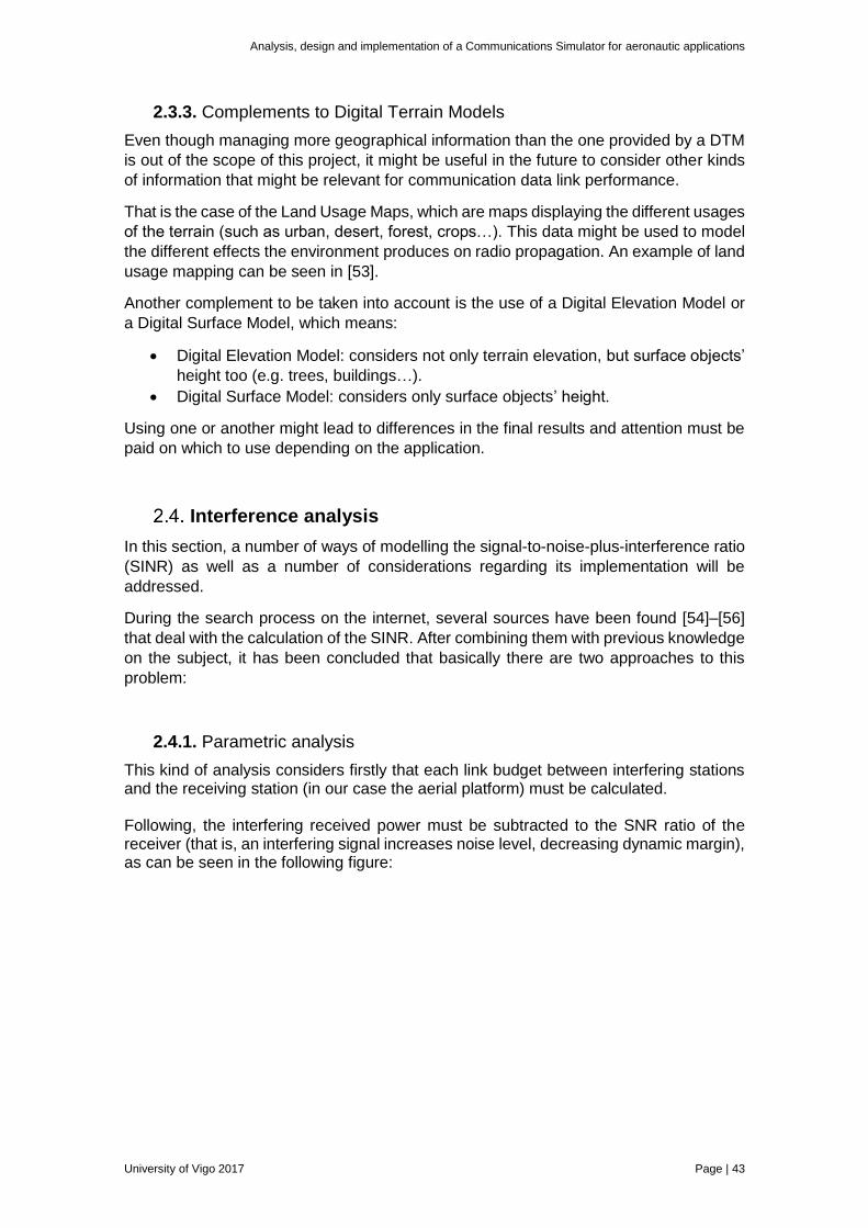
Analysis, design and implementation of a Communications Simulator for aeronautic applications
University of Vigo 2017 Page | 43
2.3.3. Complements to Digital Terrain Models
Even though managing more geographical information than the one provided by a DTM
is out of the scope of this project, it might be useful in the future to consider other kinds
of information that might be relevant for communication data link performance.
That is the case of the Land Usage Maps, which are maps displaying the different usages
of the terrain (such as urban, desert, forest, crops…). This data might be used to model
the different effects the environment produces on radio propagation. An example of land
usage mapping can be seen in [53].
Another complement to be taken into account is the use of a Digital Elevation Model or
a Digital Surface Model, which means:
Digital Elevation Model: considers not only terrain elevation, but surface objects’
height too (e.g. trees, buildings…).
Digital Surface Model: considers only surface objects’ height.
Using one or another might lead to differences in the final results and attention must be
paid on which to use depending on the application.
Interference analysis
In this section, a number of ways of modelling the signal-to-noise-plus-interference ratio
(SINR) as well as a number of considerations regarding its implementation will be
addressed.
During the search process on the internet, several sources have been found [54]–[56]
that deal with the calculation of the SINR. After combining them with previous knowledge
on the subject, it has been concluded that basically there are two approaches to this
problem:
2.4.1. Parametric analysis
This kind of analysis considers firstly that each link budget between interfering stations and the receiving station (in our case the aerial platform) must be calculated. Following, the interfering received power must be subtracted to the SNR ratio of the receiver (that is, an interfering signal increases noise level, decreasing dynamic margin), as can be seen in the following figure:
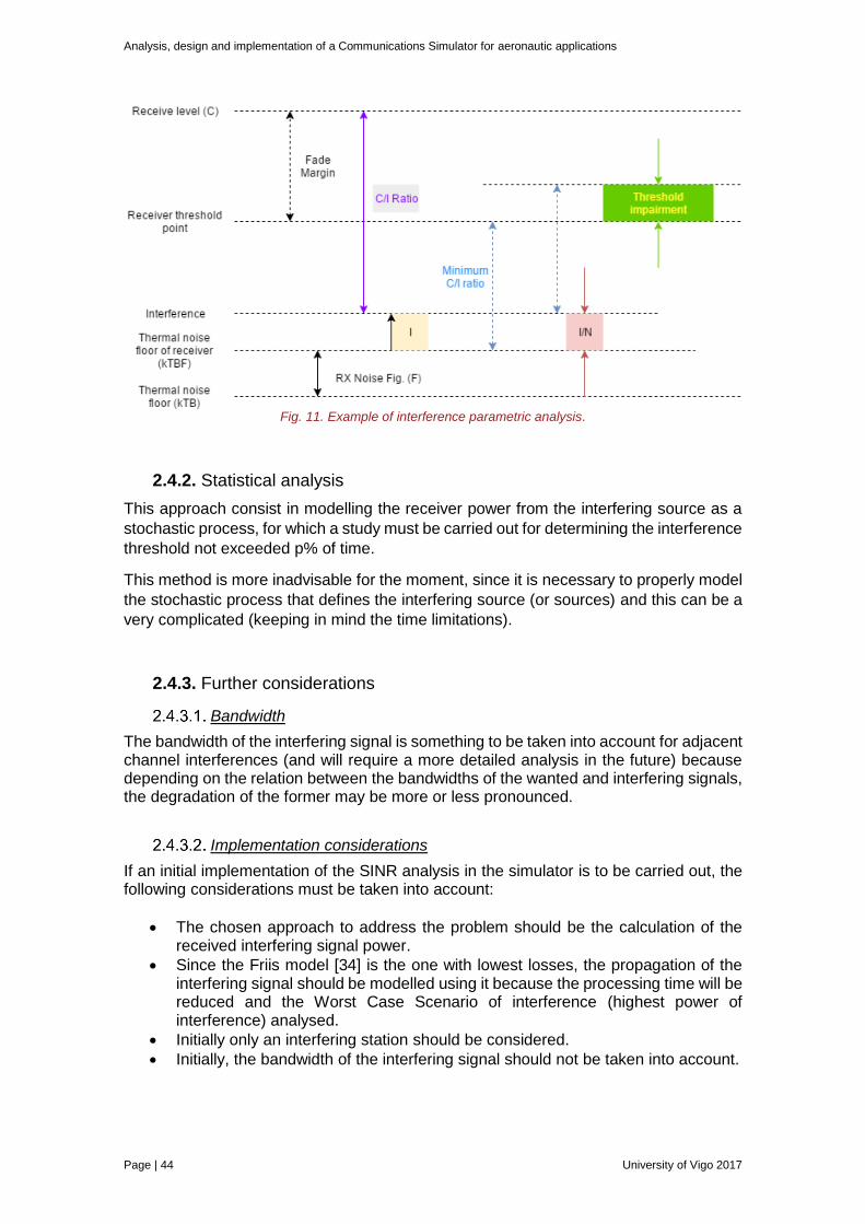
Analysis, design and implementation of a Communications Simulator for aeronautic applications
Page | 44 University of Vigo 2017
Fig. 11. Example of interference parametric analysis.
2.4.2. Statistical analysis
This approach consist in modelling the receiver power from the interfering source as a
stochastic process, for which a study must be carried out for determining the interference
threshold not exceeded p% of time.
This method is more inadvisable for the moment, since it is necessary to properly model
the stochastic process that defines the interfering source (or sources) and this can be a
very complicated (keeping in mind the time limitations).
2.4.3. Further considerations
Bandwidth
The bandwidth of the interfering signal is something to be taken into account for adjacent channel interferences (and will require a more detailed analysis in the future) because depending on the relation between the bandwidths of the wanted and interfering signals, the degradation of the former may be more or less pronounced.
Implementation considerations
If an initial implementation of the SINR analysis in the simulator is to be carried out, the following considerations must be taken into account:
The chosen approach to address the problem should be the calculation of the received interfering signal power.
Since the Friis model [34] is the one with lowest losses, the propagation of the interfering signal should be modelled using it because the processing time will be reduced and the Worst Case Scenario of interference (highest power of interference) analysed.
Initially only an interfering station should be considered.
Initially, the bandwidth of the interfering signal should not be taken into account.
Analysis, design and implementation of a Communications Simulator for aeronautic applications
University of Vigo 2017 Page | 45
Antenna radiation patterns
As it is known, an antenna does not radiate the same amount of signal over all directions,
since it follows what is called a radiation pattern [58], [59]. This phenomenon is relevant
because the gain of the antennas will be higher or lower as a function of the angle
between transmitter and receiver as a consequence off this pattern not being constant
for all directions.
Moreover, it also has to be considered the fact that at least one of the antennas (the one
placed in the aerial vehicle) will be moving, so the gain with which the signal will be
received will vary with time because of the changes in the angle between transmitter and
receiver (that, as it was said, affects the radiation pattern of both antennas).
It can be concluded that to consider the radiation pattern along a mission's path would
lead to more accurate models and thus, better mission planning.
As can be seen in [57], there are many ways to define radiation pattern files, being one
of the most common approaches to define it as a tuple of vectors following:
Vector A: antenna radiation pattern values (natural units or dB).
Vector B: vector of azimuth angle values for which the value of the radiation
pattern has been computed (degrees).
In order to consider 3D antenna radiation patterns, a third vector has to be defined:
Vector C: vector of elevation angle values for which the value of the radiation
pattern has been computed (degrees).
If necessary, some resources useful to get antenna radiation patterns are available in
[58]–[60].
Weather Forecasting
This section evaluates the considered options for adding real-time weather information
at mission area to the simulator as well as obtaining an estimate of the rain attenuation
in a mission scenario.
2.6.1. Rain attenuation modelling
In this case, the use of the rainfall model provided by the ITU in Recommendation ITU-
R p. 838-3 [61].
This model obtains an attenuation coefficient in dB / km that models the attenuation due
to rainfall as a function of the intensity of the precipitation (mm / h) and the signal
frequency ([30] shows how can be applied for frequencies below 1 GHz).
Knowing also the percentage of the route affected by the rain (or otherwise, the distance
travelled by the signal over the rain) the additional attenuation in dB can be obtained.
Therefore, it is necessary to have a source of meteorological information that not only
provides the intensity of the same, but also of its location.
Analysis, design and implementation of a Communications Simulator for aeronautic applications
Page | 46 University of Vigo 2017
2.6.2. Sources of meteorological information
In order to obtain meteorological information in Galicia region, the public Meteogalicia
API [62] can be used.
It allows direct queries to its server and returns the sky state and accumulated
precipitation during the last hour (in mm / h), which makes it a viable alternative for the
initial development of this functionality.
It has a basic spatial resolution of 4 km (which can be reduced to 1 if latitudes and
longitudes are previously discriminated to see if they fall in the ‘Rías Baixas’ or in the
‘Norte de Galicia’ regions) and a temporary resolution of one hour.
The only restriction to the use of this service is to have a free key that can be requested
by email.
In the request it can be included:
Weather information status: (SUNNY, HIGH_CLOUDS, PARTLY_CLOUDS,
OVERCAST, CLOUDY, FOG, SHOWERS, OVERCAST_AND_SHOWERS,
INTERMITENT_SNOW, DRIZZLE, RAIN, SNOW, STORMS, MIST, FOG_BANK,
MID_CLOUDS, WEAK_RAIN, WEAK_SHOWERS, STORM_THEN_CLOUDY,
MELTED_SNOW, RAIN_HAIL)
Rainfall rate in the last hour by location for up to 20 pairs of longitude and latitude
coordinates separated by ';'.
As optional parameters: output format of the requested data (.html, .gml, .kml or
.json), the model to be obtained, the grid and the time range.
It has to be remarked that in this case there is a lack of depth in the analysis but assuming
that this is a first version of the simulator, only managing data of Galicia region would be
enough.
Analysis, design and implementation of a Communications Simulator for aeronautic applications
University of Vigo 2017 Page | 47
Conclusions drawn of the state of the art
To conclude with this Chapter, several conclusions can be drawn regarding the multiple
topics or fields that has been addressed.
Firstly, it has to be noted the fact that many commercial available mission planning
software tools consider communication data link performance in their pre-mission
analysis (for example Integrasys’s AeroTrackCOM and Insitu’s ICOMC2) as was stated
in both the Abstract and the Introduction of this document.
Furthermore, reader may has had realised that most of them are intended to be used in
military applications and that for civil aircrafts flying between VOR’s, mission planning
should not be so critical. Well, while it is true commercial aviation is based on highly
controlled flight paths is a fact, there are plenty of other applications and scenarios where
paths are no so well controlled, for example: SAR operations, firefighting, surveillance
operations, aerial surveying missions and many more.
Moreover, there are not many radio propagation simulators designed for this purpose,
being the sole exception AGI’s STK software, which seems to integrate many of the
features that others lack.
At last, regarding the other elements analysed along this chapter, many considerations
has already been stated in its own sections. However, it has to be noted that all of them
might be useful, in a higher or lesser extent, for the development of a simulator intended
to be a useful tool in the future.

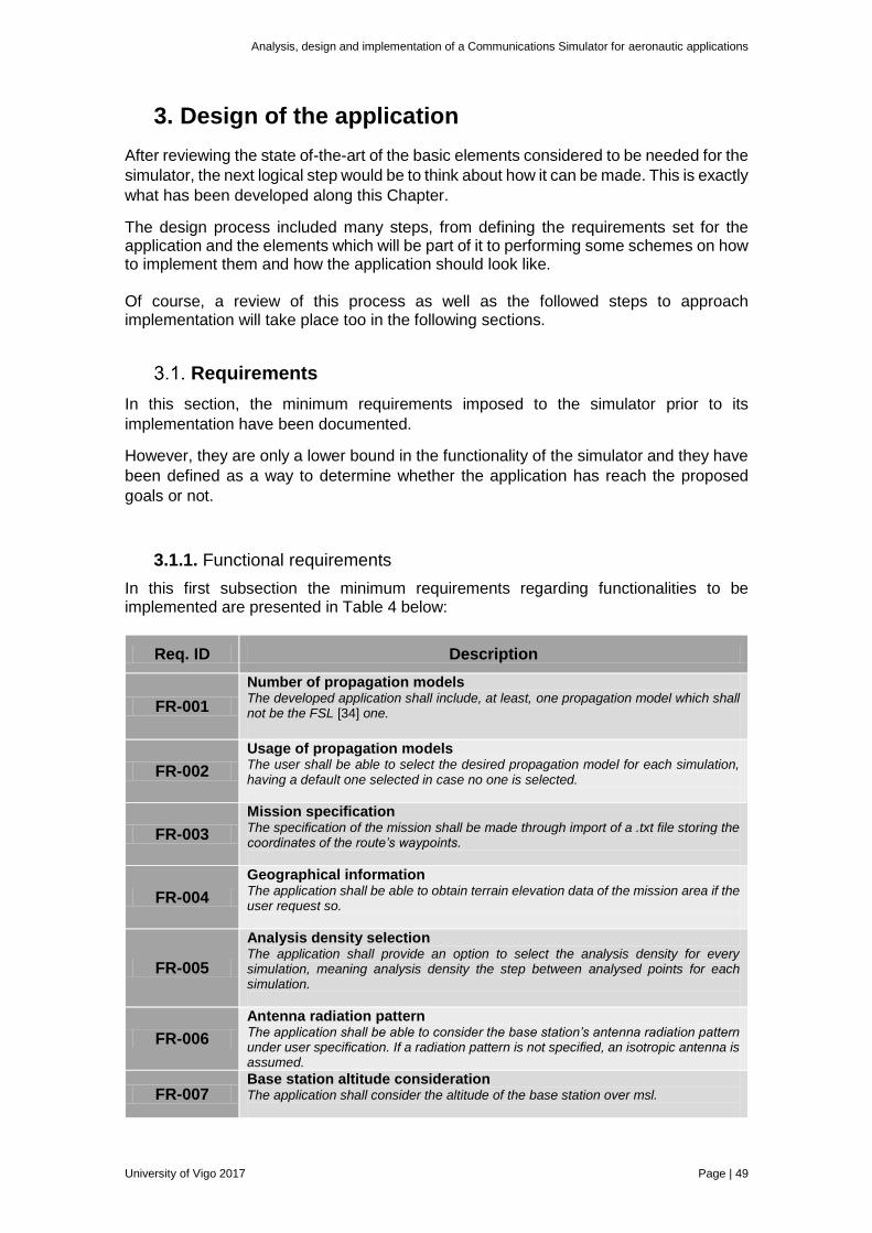
Analysis, design and implementation of a Communications Simulator for aeronautic applications
University of Vigo 2017 Page | 49
3. Design of the application
After reviewing the state of-the-art of the basic elements considered to be needed for the
simulator, the next logical step would be to think about how it can be made. This is exactly
what has been developed along this Chapter.
The design process included many steps, from defining the requirements set for the application and the elements which will be part of it to performing some schemes on how to implement them and how the application should look like. Of course, a review of this process as well as the followed steps to approach implementation will take place too in the following sections.
Requirements
In this section, the minimum requirements imposed to the simulator prior to its
implementation have been documented.
However, they are only a lower bound in the functionality of the simulator and they have
been defined as a way to determine whether the application has reach the proposed
goals or not.
3.1.1. Functional requirements
In this first subsection the minimum requirements regarding functionalities to be implemented are presented in Table 4 below:
Req. ID Description
FR-001
Number of propagation models The developed application shall include, at least, one propagation model which shall not be the FSL [34] one.
FR-002
Usage of propagation models The user shall be able to select the desired propagation model for each simulation, having a default one selected in case no one is selected.
FR-003
Mission specification The specification of the mission shall be made through import of a .txt file storing the coordinates of the route’s waypoints.
FR-004
Geographical information The application shall be able to obtain terrain elevation data of the mission area if the user request so.
FR-005
Analysis density selection The application shall provide an option to select the analysis density for every simulation, meaning analysis density the step between analysed points for each simulation.
FR-006
Antenna radiation pattern The application shall be able to consider the base station’s antenna radiation pattern under user specification. If a radiation pattern is not specified, an isotropic antenna is assumed.
FR-007 Base station altitude consideration The application shall consider the altitude of the base station over msl.
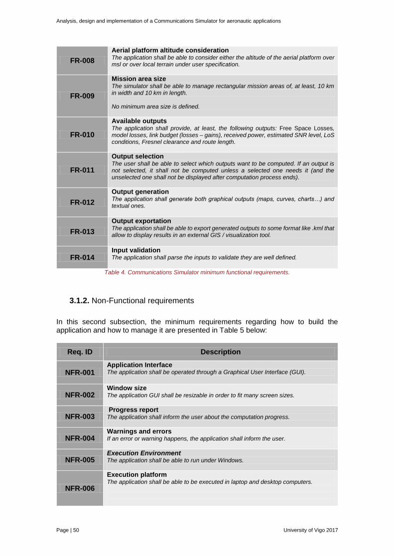
Analysis, design and implementation of a Communications Simulator for aeronautic applications
Page | 50 University of Vigo 2017
FR-008
Aerial platform altitude consideration The application shall be able to consider either the altitude of the aerial platform over msl or over local terrain under user specification.
FR-009
Mission area size The simulator shall be able to manage rectangular mission areas of, at least, 10 km in width and 10 km in length. No minimum area size is defined.
FR-010
Available outputs
The application shall provide, at least, the following outputs: Free Space Losses, model losses, link budget (losses – gains), received power, estimated SNR level, LoS conditions, Fresnel clearance and route length.
FR-011
Output selection The user shall be able to select which outputs want to be computed. If an output is not selected, it shall not be computed unless a selected one needs it (and the unselected one shall not be displayed after computation process ends).
FR-012
Output generation The application shall generate both graphical outputs (maps, curves, charts…) and textual ones.
FR-013
Output exportation The application shall be able to export generated outputs to some format like .kml that allow to display results in an external GIS / visualization tool.
FR-014 Input validation The application shall parse the inputs to validate they are well defined.
Table 4. Communications Simulator minimum functional requirements.
3.1.2. Non-Functional requirements
In this second subsection, the minimum requirements regarding how to build the application and how to manage it are presented in Table 5 below:
Req. ID Description
NFR-001 Application Interface The application shall be operated through a Graphical User Interface (GUI).
NFR-002 Window size The application GUI shall be resizable in order to fit many screen sizes.
NFR-003 Progress report The application shall inform the user about the computation progress.
NFR-004 Warnings and errors If an error or warning happens, the application shall inform the user.
NFR-005 Execution Environment The application shall be able to run under Windows.
NFR-006
Execution platform
The application shall be able to be executed in laptop and desktop computers.
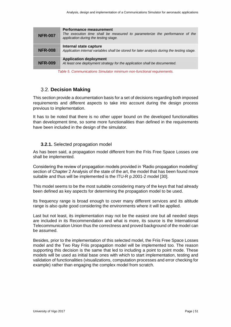
Analysis, design and implementation of a Communications Simulator for aeronautic applications
University of Vigo 2017 Page | 51
NFR-007
Performance measurement The execution time shall be measured to parameterize the performance of the application during the testing stage.
NFR-008 Internal state capture Application internal variables shall be stored for later analysis during the testing stage.
NFR-009 Application deployment At least one deployment strategy for the application shall be documented.
Table 5. Communications Simulator minimum non-functional requirements.
Decision Making
This section provide a documentation basis for a set of decisions regarding both imposed
requirements and different aspects to take into account during the design process
previous to implementation.
It has to be noted that there is no other upper bound on the developed functionalities
than development time, so some more functionalities than defined in the requirements
have been included in the design of the simulator.
3.2.1. Selected propagation model
As has been said, a propagation model different from the Friis Free Space Losses one shall be implemented. Considering the review of propagation models provided in ‘Radio propagation modelling’ section of Chapter 2 Analysis of the state of the art, the model that has been found more suitable and thus will be implemented is the ITU-R p.2001-2 model [30]. This model seems to be the most suitable considering many of the keys that had already been defined as key aspects for determining the propagation model to be used. Its frequency range is broad enough to cover many different services and its altitude range is also quite good considering the environments where it will be applied. Last but not least, its implementation may not be the easiest one but all needed steps are included in its Recommendation and what is more, its source is the International Telecommunication Union thus the correctness and proved background of the model can be assumed. Besides, prior to the implementation of this selected model, the Friis Free Space Losses model and the Two Ray Friis propagation model will be implemented too. The reason supporting this decision is the same that led to including a point to point mode. These models will be used as initial base ones with which to start implementation, testing and validation of functionalities (visualizations, computation processes and error checking for example) rather than engaging the complex model from scratch.
Analysis, design and implementation of a Communications Simulator for aeronautic applications
Page | 52 University of Vigo 2017
3.2.2. Selected Digital Terrain Model
The DTM provided by 'Instituto Geográfico Nacional', with a base accuracy of 25 meters, available data of all Spain and capability to serve HTTP queries fits the needs of the project. With reasons provided, the Digital Terrain Model which will be queried has been selected. The main implementation workload for this element will be to develop a method to automatically generate the queries, to send them to the server and also to process and use the received data.
3.2.3. Selected modes of operation
At this point, it has been decided to implement four different modes of operation:
Point to Point Mode
Route Mode
Area Prediction Mode
Satellite Mode In the following paragraphs, this four modes will be described including also the given reasons to implement each one of them.
Point to Point Mode
This mode consists in compute the link budget between two points, transmitter and
receiver, not considering that receiver will be moving.
The main reason behind the decision of implementing this mode is the will to have a
‘quick’ test mode over which to implement the different propagation models and
functionalities the Simulator will have in an easier way than to implement the route mode
from scratch.
The other modes are developed taking this one as their basis.
In addition, as can be found on section ‘Radio propagation simulators’ from Chapter
2Analysis of the state of the art, this mode is a common tool in radio network planning,
so this can be seen as an added value for this or other related projects, being useful
when a simple link state should be evaluated.
Route Mode
This is one of the main modes of the simulator (and a minimum requirement too). Given
the location of the base station and the path followed by the aerial platform, an analysis
on the communications’ link state along all route will be performed.
Area Prediction Mode
This mode, derived from the previous one, assumes a known base station location and
an area where the aerial platform shall be, without having knowledge on the exact path
followed by it.
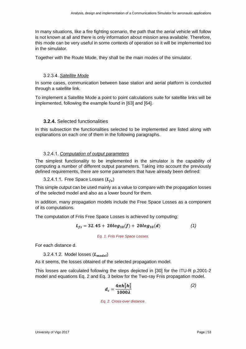
Analysis, design and implementation of a Communications Simulator for aeronautic applications
University of Vigo 2017 Page | 53
In many situations, like a fire fighting scenario, the path that the aerial vehicle will follow
is not known at all and there is only information about mission area available. Therefore,
this mode can be very useful in some contexts of operation so it will be implemented too
in the simulator.
Together with the Route Mode, they shall be the main modes of the simulator.
Satellite Mode
In some cases, communication between base station and aerial platform is conducted
through a satellite link.
To implement a Satellite Mode a point to point calculations suite for satellite links will be
implemented, following the example found in [63] and [64].
3.2.4. Selected functionalities
In this subsection the functionalities selected to be implemented are listed along with explanations on each one of them in the following paragraphs.
Computation of output parameters
The simplest functionality to be implemented in the simulator is the capability of computing a number of different output parameters. Taking into account the previously defined requirements, there are some parameters that have already been defined:
Free Space Losses (𝑳𝒇𝒔)
This simple output can be used mainly as a value to compare with the propagation losses
of the selected model and also as a lower bound for them.
In addition, many propagation models include the Free Space Losses as a component
of its computations.
The computation of Friis Free Space Losses is achieved by computing:
𝑳𝒇𝒔 = 𝟑𝟐. 𝟒𝟓 + 𝟐𝟎𝒍𝒐𝒈𝟏𝟎(𝒇) + 𝟐𝟎𝒍𝒐𝒈𝟏𝟎(𝒅) (1)
Eq. 1. Friis Free Space Losses.
For each distance d.
Model losses (𝑳𝒎𝒐𝒅𝒆𝒍)
As it seems, the losses obtained of the selected propagation model.
This losses are calculated following the steps depicted in [30] for the ITU-R p.2001-2
model and equations Eq. 2 and Eq. 3 below for the Two-ray Friis propagation model.
𝒅𝒄 =𝟒𝝅𝒉𝟏
𝟐𝒉𝟐𝟐
𝟏𝟎𝟎𝟎𝝀
(2)
Eq. 2. Cross-over distance.
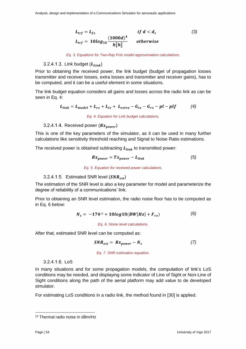
Analysis, design and implementation of a Communications Simulator for aeronautic applications
Page | 54 University of Vigo 2017
𝑳𝒕𝒓𝒇 = 𝑳𝒇𝒔 𝒊𝒇 𝒅 < 𝒅𝒄
𝑳𝒕𝒓𝒇 = 𝟏𝟎𝒍𝒐𝒈𝟏𝟎
(𝟏𝟎𝟎𝟎𝒅)𝟒
𝒉𝟏𝟐𝒉𝟐
𝟐 𝒐𝒕𝒉𝒆𝒓𝒘𝒊𝒔𝒆
(3)
Eq. 3. Equations for Two-Ray Friis model approximation calculations.
Link budget (𝑳𝑳𝒊𝒏𝒌)
Prior to obtaining the received power, the link budget (budget of propagation losses
transmitter and receiver losses, extra losses and transmitter and receiver gains), has to
be computed, and it can be a useful element in some situations.
The link budget equation considers all gains and losses across the radio link as can be
seen in Eq. 4:
𝑳𝒍𝒊𝒏𝒌 = 𝑳𝒎𝒐𝒅𝒆𝒍 + 𝑳𝒓𝒙 + 𝑳𝒕𝒙 + 𝑳𝒆𝒙𝒕𝒓𝒂 − 𝑮𝒕𝒙 − 𝑮𝒓𝒙 − 𝒑𝒍 − 𝒑𝒍𝒇 (4)
Eq. 4. Equation for Link budget calculations.
Received power (𝑹𝒙𝒑𝒐𝒘𝒆𝒓)
This is one of the key parameters of the simulator, as it can be used in many further
calculations like sensitivity threshold reaching and Signal to Noise Ratio estimations.
The received power is obtained subtracting 𝑳𝒍𝒊𝒏𝒌 to transmitted power:
𝑹𝒙𝒑𝒐𝒘𝒆𝒓 = 𝑻𝒙𝒑𝒐𝒘𝒆𝒓 − 𝑳𝒍𝒊𝒏𝒌 (5)
Eq. 5. Equation for received power calculations.
Estimated SNR level (𝑺𝑵𝑹𝒆𝒔𝒕)
The estimation of the SNR level is also a key parameter for model and parameterize the
degree of reliability of a communications’ link.
Prior to obtaining an SNR level estimation, the radio noise floor has to be computed as
in Eq. 6 below:
𝑵𝒔 = −𝟏𝟕𝟒15 + 𝟏𝟎𝒍𝒐𝒈𝟏𝟎(𝑩𝑾[𝑯𝒛] + 𝑭𝒓𝒙)
(6)
Eq. 6. Noise level calculations.
After that, estimated SNR level can be computed as:
𝑺𝑵𝑹𝒆𝒔𝒕 = 𝑹𝒙𝒑𝒐𝒘𝒆𝒓 − 𝑵𝒔
(7)
Eq. 7. SNR estimation equation.
LoS
In many situations and for some propagation models, the computation of link’s LoS
conditions may be needed, and displaying some indicator of Line of Sight or Non-Line of
Sight conditions along the path of the aerial platform may add value to de developed
simulator.
For estimating LoS conditions in a radio link, the method found in [30] is applied.
15 Thermal radio noise in dBm/Hz
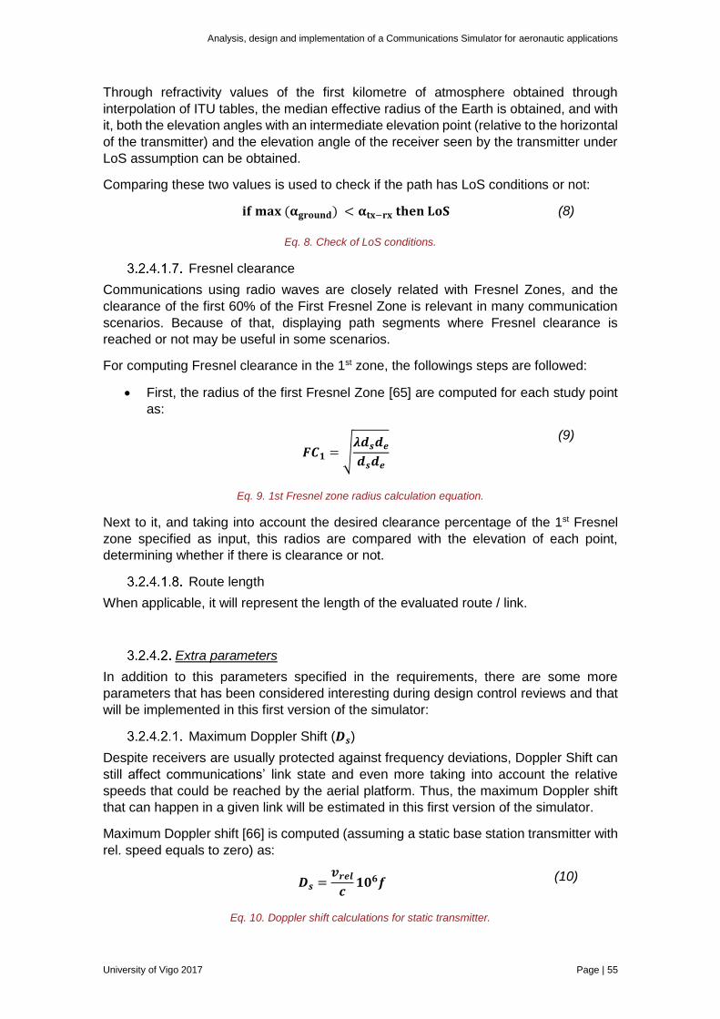
Analysis, design and implementation of a Communications Simulator for aeronautic applications
University of Vigo 2017 Page | 55
Through refractivity values of the first kilometre of atmosphere obtained through
interpolation of ITU tables, the median effective radius of the Earth is obtained, and with
it, both the elevation angles with an intermediate elevation point (relative to the horizontal
of the transmitter) and the elevation angle of the receiver seen by the transmitter under
LoS assumption can be obtained.
Comparing these two values is used to check if the path has LoS conditions or not:
𝐢𝐟 𝐦𝐚𝐱 (𝛂𝐠𝐫𝐨𝐮𝐧𝐝) < 𝛂𝐭𝐱−𝐫𝐱 𝐭𝐡𝐞𝐧 𝐋𝐨𝐒 (8)
Eq. 8. Check of LoS conditions.
Fresnel clearance
Communications using radio waves are closely related with Fresnel Zones, and the
clearance of the first 60% of the First Fresnel Zone is relevant in many communication
scenarios. Because of that, displaying path segments where Fresnel clearance is
reached or not may be useful in some scenarios.
For computing Fresnel clearance in the 1st zone, the followings steps are followed:
First, the radius of the first Fresnel Zone [65] are computed for each study point
as:
𝑭𝑪𝟏 = √𝝀𝒅𝒔𝒅𝒆
𝒅𝒔𝒅𝒆
(9)
Eq. 9. 1st Fresnel zone radius calculation equation.
Next to it, and taking into account the desired clearance percentage of the 1st Fresnel
zone specified as input, this radios are compared with the elevation of each point,
determining whether if there is clearance or not.
Route length
When applicable, it will represent the length of the evaluated route / link.
Extra parameters
In addition to this parameters specified in the requirements, there are some more
parameters that has been considered interesting during design control reviews and that
will be implemented in this first version of the simulator:
Maximum Doppler Shift (𝑫𝒔)
Despite receivers are usually protected against frequency deviations, Doppler Shift can
still affect communications’ link state and even more taking into account the relative
speeds that could be reached by the aerial platform. Thus, the maximum Doppler shift
that can happen in a given link will be estimated in this first version of the simulator.
Maximum Doppler shift [66] is computed (assuming a static base station transmitter with
rel. speed equals to zero) as:
𝑫𝒔 =𝒗𝒓𝒆𝒍
𝒄𝟏𝟎𝟔𝒇 (10)
Eq. 10. Doppler shift calculations for static transmitter.
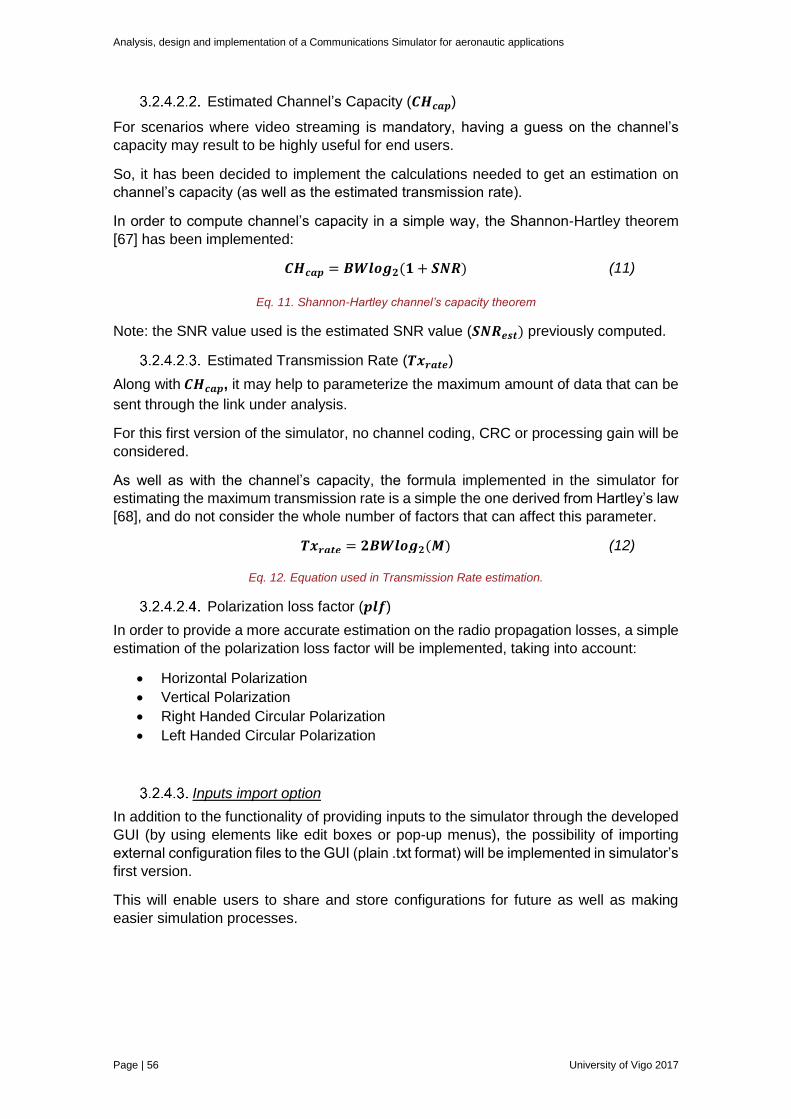
Analysis, design and implementation of a Communications Simulator for aeronautic applications
Page | 56 University of Vigo 2017
Estimated Channel’s Capacity (𝑪𝑯𝒄𝒂𝒑)
For scenarios where video streaming is mandatory, having a guess on the channel’s
capacity may result to be highly useful for end users.
So, it has been decided to implement the calculations needed to get an estimation on
channel’s capacity (as well as the estimated transmission rate).
In order to compute channel’s capacity in a simple way, the Shannon-Hartley theorem
[67] has been implemented:
𝑪𝑯𝒄𝒂𝒑 = 𝑩𝑾𝒍𝒐𝒈𝟐(𝟏 + 𝑺𝑵𝑹) (11)
Eq. 11. Shannon-Hartley channel’s capacity theorem
Note: the SNR value used is the estimated SNR value (𝑺𝑵𝑹𝒆𝒔𝒕) previously computed.
Estimated Transmission Rate (𝑻𝒙𝒓𝒂𝒕𝒆)
Along with 𝑪𝑯𝒄𝒂𝒑, it may help to parameterize the maximum amount of data that can be
sent through the link under analysis.
For this first version of the simulator, no channel coding, CRC or processing gain will be
considered.
As well as with the channel’s capacity, the formula implemented in the simulator for
estimating the maximum transmission rate is a simple the one derived from Hartley’s law
[68], and do not consider the whole number of factors that can affect this parameter.
𝑻𝒙𝒓𝒂𝒕𝒆 = 𝟐𝑩𝑾𝒍𝒐𝒈𝟐(𝑴) (12)
Eq. 12. Equation used in Transmission Rate estimation.
Polarization loss factor (𝒑𝒍𝒇)
In order to provide a more accurate estimation on the radio propagation losses, a simple
estimation of the polarization loss factor will be implemented, taking into account:
Horizontal Polarization
Vertical Polarization
Right Handed Circular Polarization
Left Handed Circular Polarization
Inputs import option
In addition to the functionality of providing inputs to the simulator through the developed
GUI (by using elements like edit boxes or pop-up menus), the possibility of importing
external configuration files to the GUI (plain .txt format) will be implemented in simulator’s
first version.
This will enable users to share and store configurations for future as well as making
easier simulation processes.
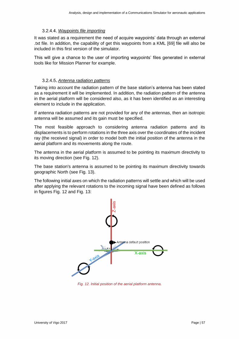
Analysis, design and implementation of a Communications Simulator for aeronautic applications
University of Vigo 2017 Page | 57
Waypoints file importing
It was stated as a requirement the need of acquire waypoints’ data through an external
.txt file. In addition, the capability of get this waypoints from a KML [69] file will also be
included in this first version of the simulator.
This will give a chance to the user of importing waypoints’ files generated in external
tools like for Mission Planner for example.
Antenna radiation patterns
Taking into account the radiation pattern of the base station’s antenna has been stated
as a requirement it will be implemented. In addition, the radiation pattern of the antenna
in the aerial platform will be considered also, as it has been identified as an interesting
element to include in the application.
If antenna radiation patterns are not provided for any of the antennas, then an isotropic
antenna will be assumed and its gain must be specified.
The most feasible approach to considering antenna radiation patterns and its
displacements is to perform rotations in the three axis over the coordinates of the incident
ray (the received signal) in order to model both the initial position of the antenna in the
aerial platform and its movements along the route.
The antenna in the aerial platform is assumed to be pointing its maximum directivity to
its moving direction (see Fig. 12).
The base station's antenna is assumed to be pointing its maximum directivity towards
geographic North (see Fig. 13).
The following initial axes on which the radiation patterns will settle and which will be used
after applying the relevant rotations to the incoming signal have been defined as follows
in figures Fig. 12 and Fig. 13:
Fig. 12. Initial position of the aerial platform antenna.
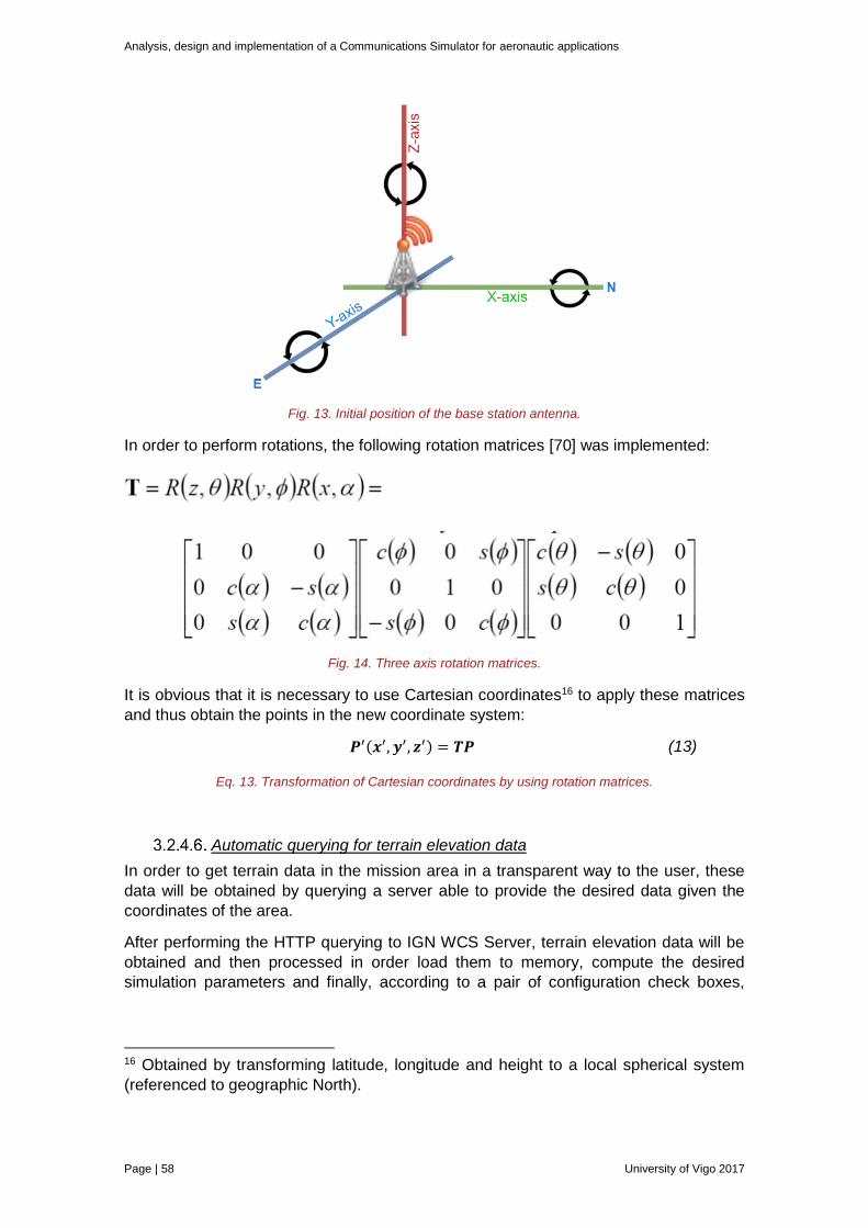
Analysis, design and implementation of a Communications Simulator for aeronautic applications
Page | 58 University of Vigo 2017
Fig. 13. Initial position of the base station antenna.
In order to perform rotations, the following rotation matrices [70] was implemented:
Fig. 14. Three axis rotation matrices.
It is obvious that it is necessary to use Cartesian coordinates16 to apply these matrices
and thus obtain the points in the new coordinate system:
𝑷′(𝒙′, 𝒚′, 𝒛′) = 𝑻𝑷 (13)
Eq. 13. Transformation of Cartesian coordinates by using rotation matrices.
Automatic querying for terrain elevation data
In order to get terrain data in the mission area in a transparent way to the user, these
data will be obtained by querying a server able to provide the desired data given the
coordinates of the area.
After performing the HTTP querying to IGN WCS Server, terrain elevation data will be
obtained and then processed in order load them to memory, compute the desired
simulation parameters and finally, according to a pair of configuration check boxes,
16 Obtained by transforming latitude, longitude and height to a local spherical system
(referenced to geographic North).
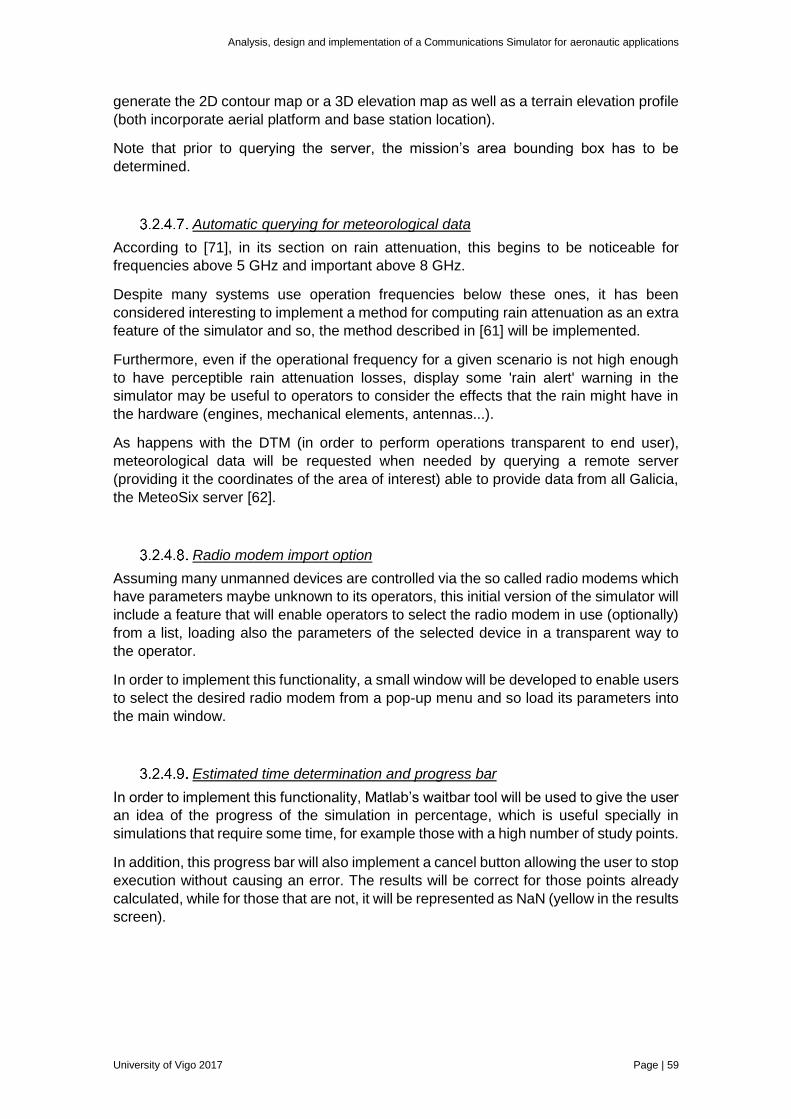
Analysis, design and implementation of a Communications Simulator for aeronautic applications
University of Vigo 2017 Page | 59
generate the 2D contour map or a 3D elevation map as well as a terrain elevation profile
(both incorporate aerial platform and base station location).
Note that prior to querying the server, the mission’s area bounding box has to be
determined.
Automatic querying for meteorological data
According to [71], in its section on rain attenuation, this begins to be noticeable for
frequencies above 5 GHz and important above 8 GHz.
Despite many systems use operation frequencies below these ones, it has been
considered interesting to implement a method for computing rain attenuation as an extra
feature of the simulator and so, the method described in [61] will be implemented.
Furthermore, even if the operational frequency for a given scenario is not high enough
to have perceptible rain attenuation losses, display some 'rain alert' warning in the
simulator may be useful to operators to consider the effects that the rain might have in
the hardware (engines, mechanical elements, antennas...).
As happens with the DTM (in order to perform operations transparent to end user),
meteorological data will be requested when needed by querying a remote server
(providing it the coordinates of the area of interest) able to provide data from all Galicia,
the MeteoSix server [62].
Radio modem import option
Assuming many unmanned devices are controlled via the so called radio modems which
have parameters maybe unknown to its operators, this initial version of the simulator will
include a feature that will enable operators to select the radio modem in use (optionally)
from a list, loading also the parameters of the selected device in a transparent way to
the operator.
In order to implement this functionality, a small window will be developed to enable users
to select the desired radio modem from a pop-up menu and so load its parameters into
the main window.
Estimated time determination and progress bar
In order to implement this functionality, Matlab’s waitbar tool will be used to give the user
an idea of the progress of the simulation in percentage, which is useful specially in
simulations that require some time, for example those with a high number of study points.
In addition, this progress bar will also implement a cancel button allowing the user to stop
execution without causing an error. The results will be correct for those points already
calculated, while for those that are not, it will be represented as NaN (yellow in the results
screen).
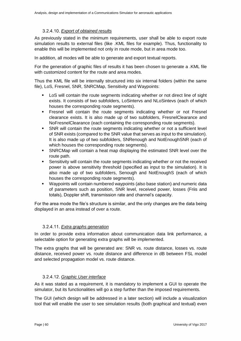
Analysis, design and implementation of a Communications Simulator for aeronautic applications
Page | 60 University of Vigo 2017
Export of obtained results
As previously stated in the minimum requirements, user shall be able to export route
simulation results to external files (like .KML files for example). Thus, functionality to
enable this will be implemented not only in route mode, but in area mode too.
In addition, all modes will be able to generate and export textual reports.
For the generation of graphic files of results it has been chosen to generate a .KML file
with customized content for the route and area modes.
Thus the KML file will be internally structured into six internal folders (within the same
file), LoS, Fresnel, SNR, SNRCMap, Sensitivity and Waypoints:
LoS will contain the route segments indicating whether or not direct line of sight
exists. It consists of two subfolders, LoSintervs and NLoSintevs (each of which
houses the corresponding route segments).
Fresnel will contain the route segments indicating whether or not Fresnel
clearance exists. It is also made up of two subfolders, FresnelClearance and
NoFresnelClearance (each containing the corresponding route segments).
SNR will contain the route segments indicating whether or not a sufficient level
of SNR exists (compared to the SNR value that serves as input to the simulation).
It is also made up of two subfolders, SNRenough and NotEnoughSNR (each of
which houses the corresponding route segments).
SNRCMap will contain a heat map displaying the estimated SNR level over the
route path.
Sensitivity will contain the route segments indicating whether or not the received
power is above sensitivity threshold (specified as input to the simulation). It is
also made up of two subfolders, Senough and NotEnoughS (each of which
houses the corresponding route segments).
Waypoints will contain numbered waypoints (also base station) and numeric data
of parameters such as position, SNR level, received power, losses (Friis and
totals), Doppler shift, transmission rate and channel’s capacity.
For the area mode the file’s structure is similar, and the only changes are the data being
displayed in an area instead of over a route.
Extra graphs generation
In order to provide extra information about communication data link performance, a
selectable option for generating extra graphs will be implemented.
The extra graphs that will be generated are: SNR vs. route distance, losses vs. route
distance, received power vs. route distance and difference in dB between FSL model
and selected propagation model vs. route distance.
Graphic User interface
As it was stated as a requirement, it is mandatory to implement a GUI to operate the
simulator, but its functionalities will go a step further than the imposed requirements.
The GUI (which design will be addressed in a later section) will include a visualization
tool that will enable the user to see simulation results (both graphical and textual) even
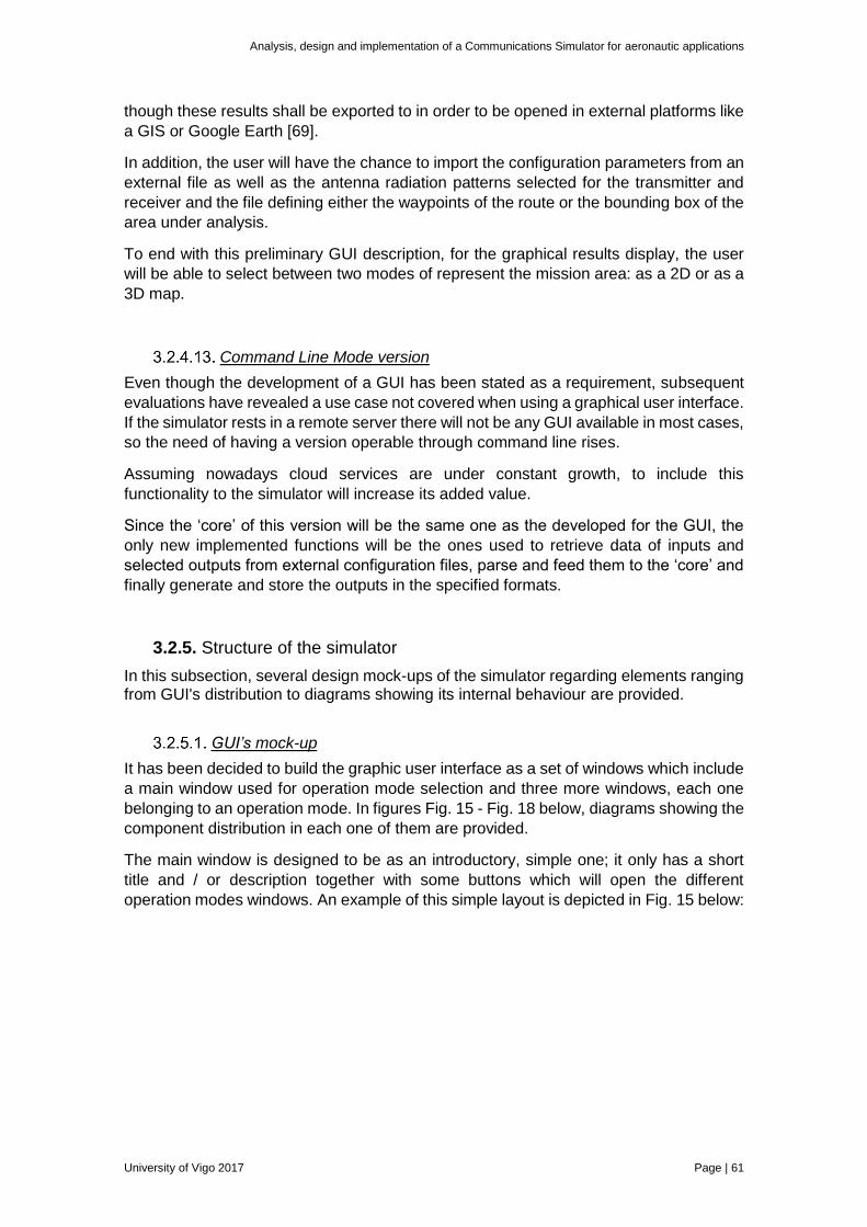
Analysis, design and implementation of a Communications Simulator for aeronautic applications
University of Vigo 2017 Page | 61
though these results shall be exported to in order to be opened in external platforms like
a GIS or Google Earth [69].
In addition, the user will have the chance to import the configuration parameters from an
external file as well as the antenna radiation patterns selected for the transmitter and
receiver and the file defining either the waypoints of the route or the bounding box of the
area under analysis.
To end with this preliminary GUI description, for the graphical results display, the user
will be able to select between two modes of represent the mission area: as a 2D or as a
3D map.
Command Line Mode version
Even though the development of a GUI has been stated as a requirement, subsequent
evaluations have revealed a use case not covered when using a graphical user interface.
If the simulator rests in a remote server there will not be any GUI available in most cases,
so the need of having a version operable through command line rises.
Assuming nowadays cloud services are under constant growth, to include this
functionality to the simulator will increase its added value.
Since the ‘core’ of this version will be the same one as the developed for the GUI, the
only new implemented functions will be the ones used to retrieve data of inputs and
selected outputs from external configuration files, parse and feed them to the ‘core’ and
finally generate and store the outputs in the specified formats.
3.2.5. Structure of the simulator
In this subsection, several design mock-ups of the simulator regarding elements ranging from GUI's distribution to diagrams showing its internal behaviour are provided.
GUI’s mock-up
It has been decided to build the graphic user interface as a set of windows which include
a main window used for operation mode selection and three more windows, each one
belonging to an operation mode. In figures Fig. 15 - Fig. 18 below, diagrams showing the
component distribution in each one of them are provided.
The main window is designed to be as an introductory, simple one; it only has a short
title and / or description together with some buttons which will open the different
operation modes windows. An example of this simple layout is depicted in Fig. 15 below:
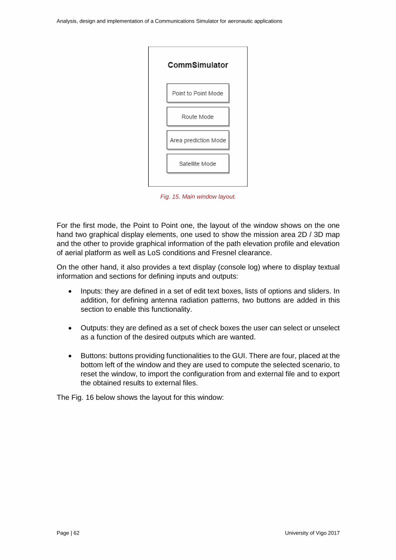
Analysis, design and implementation of a Communications Simulator for aeronautic applications
Page | 62 University of Vigo 2017
Fig. 15. Main window layout.
For the first mode, the Point to Point one, the layout of the window shows on the one
hand two graphical display elements, one used to show the mission area 2D / 3D map
and the other to provide graphical information of the path elevation profile and elevation
of aerial platform as well as LoS conditions and Fresnel clearance.
On the other hand, it also provides a text display (console log) where to display textual
information and sections for defining inputs and outputs:
Inputs: they are defined in a set of edit text boxes, lists of options and sliders. In
addition, for defining antenna radiation patterns, two buttons are added in this
section to enable this functionality.
Outputs: they are defined as a set of check boxes the user can select or unselect
as a function of the desired outputs which are wanted.
Buttons: buttons providing functionalities to the GUI. There are four, placed at the
bottom left of the window and they are used to compute the selected scenario, to
reset the window, to import the configuration from and external file and to export
the obtained results to external files.
The Fig. 16 below shows the layout for this window:
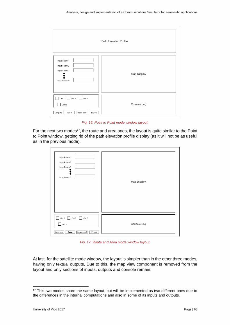
Analysis, design and implementation of a Communications Simulator for aeronautic applications
University of Vigo 2017 Page | 63
Fig. 16. Point to Point mode window layout.
For the next two modes17, the route and area ones, the layout is quite similar to the Point
to Point window, getting rid of the path elevation profile display (as it will not be as useful
as in the previous mode).
Fig. 17. Route and Area mode window layout.
At last, for the satellite mode window, the layout is simpler than in the other three modes,
having only textual outputs. Due to this, the map view component is removed from the
layout and only sections of inputs, outputs and console remain.
17 This two modes share the same layout, but will be implemented as two different ones due to the differences in the internal computations and also in some of its inputs and outputs.
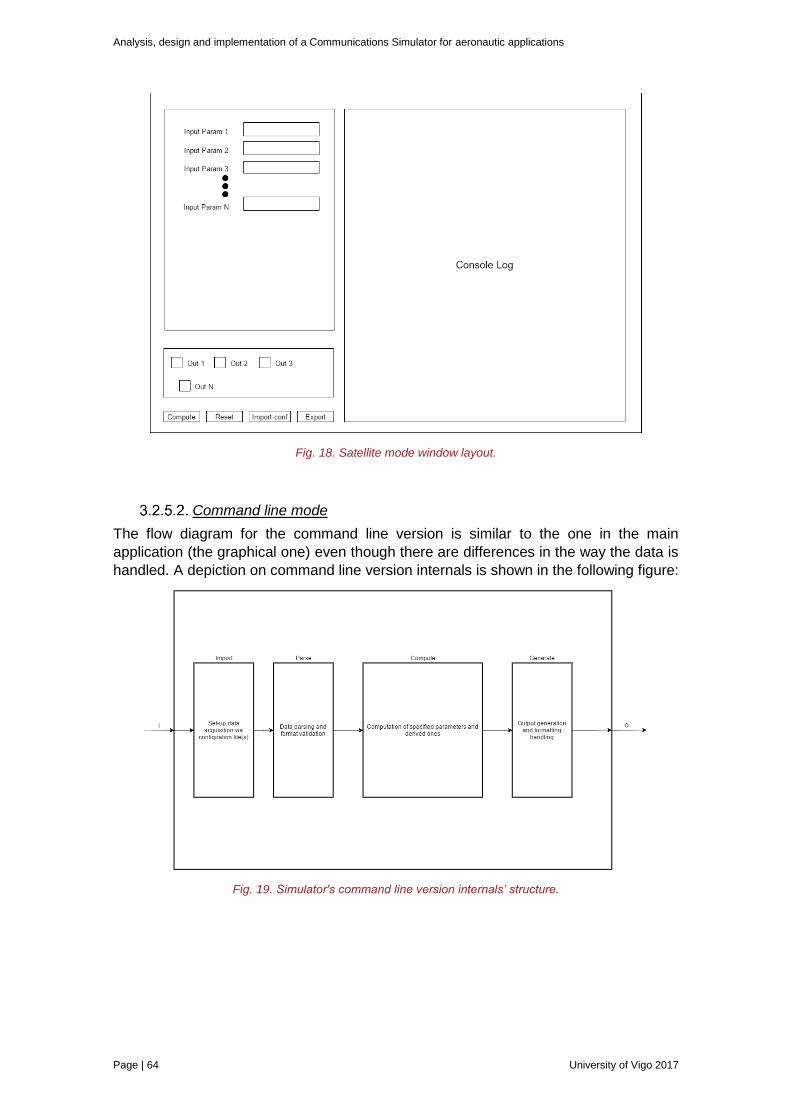
Analysis, design and implementation of a Communications Simulator for aeronautic applications
Page | 64 University of Vigo 2017
Fig. 18. Satellite mode window layout.
Command line mode
The flow diagram for the command line version is similar to the one in the main
application (the graphical one) even though there are differences in the way the data is
handled. A depiction on command line version internals is shown in the following figure:
Fig. 19. Simulator's command line version internals’ structure.

Analysis, design and implementation of a Communications Simulator for aeronautic applications
University of Vigo 2017 Page | 65
Approach to design process
This section aims to provide a brief description on project's design process, enabling the
reader to know its basis.
Among the tasks carried out, the following may be included:
To select the candidate functionalities to be implemented.
To define the different operation modes of the simulator, considering the different
applications that can be covered by each one.
To choose the Digital Terrain Model which better fits project's needs.
To generate the layouts of the different window(s) that integrate the GUI.
To plan the flow diagrams of the different operation modes.
To provide the reasons supporting the decisions of the previous elements
To write all information relevant to design process.
3.3.1. Steps of design process
In the following paragraphs, a short description on the followed steps during the design
process is provided.
Step 0: to establish the minimum requirements imposed to the developed
application.
Step 1: to manage all available information (collected in the state of the art) of a
particular field and determine what extra features to include in the simulator and
how to implement the finally selected ones.
Step 2: to document and to reason why the selected element(s) in Step 1 has
(have) to be included.
Step 3: to evaluate taken decisions, to consider modifications and to perform
them in some cases.
Step 4: to repeat Steps 1, 2 and 3 for all information fields available.
Step 5: design the different mode's windows.
Step 6 final review of design, just before to begin the implementation's process.

Analysis, design and implementation of a Communications Simulator for aeronautic applications
University of Vigo 2017 Page | 67
4. Implementation of the prototype and verification
process
This 4th Chapter presents the implementation process of the simulator, as well as the
followed verification process.
Several topics are addressed in the sections below, ranging from a description on the
programming language selected, a summary of the inputs and outputs defined for the
simulator and the implementation process itself to a short review on the verification and
testing of the simulator.
Selected implementation language
Since the design process was independent of the used programming language, here a
short discussion on the different programming languages available prior to selection of
the implementation language takes place.
In first instance it was considered the possibility of developing the simulator on Matlab,
but now it is time to justify this decision and to check if there are better alternatives, the
pros and cons of each one.
Although it is true that some of the commercial software analysed previously based their
implementation in C++, it is necessary to say that in this case (quite computational load,
handling of large amounts of data and cumbersome formulas) may not be the best
alternative to begin the development, not so for a possible later development.
Moreover, since many GIS [72], [73] nowadays support the integration of Python-based
plugins it might be also a good approach for a commercial version of the simulator. This
would relieve many tasks related with visualization and data representation but the main
drawback is the time needed to learn about the interaction of this platforms with Python
and the limitations on the functionalities that can be implemented, which both have not
been determined.
In this aspect Matlab is harmed, especially by the lack of ability to create an application
not dependent on the program's work environment or its calculation engine.
However, regarding the current situation: being in a development stage (having limited
time) it has been considered that the use of Matlab is the best option due to the large
number of Built-in18 functions that it provides through its core and that can be expanded
by multiple Toolboxes if needed.
Taking into account the previous statements, as well as its easy management of data
structures (arrays, matrices, structures...) the decision become, a priori, more correct
always bearing in mind the need to port the code sooner or later if the development of
the simulator keeps going further steps.
18 It is necessary to take into account 'the shadows' behind these tools: when porting the code to another language, with every built-in function which have been used, harder the process will be because it will be needed to begin from scratch with them instead of simply translating them.
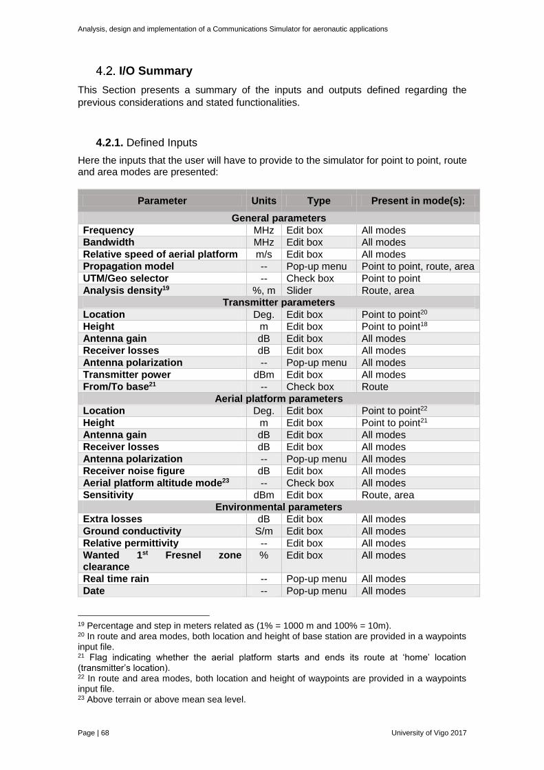
Analysis, design and implementation of a Communications Simulator for aeronautic applications
Page | 68 University of Vigo 2017
I/O Summary
This Section presents a summary of the inputs and outputs defined regarding the
previous considerations and stated functionalities.
4.2.1. Defined Inputs
Here the inputs that the user will have to provide to the simulator for point to point, route and area modes are presented:
Parameter Units Type Present in mode(s):
General parameters
Frequency MHz Edit box All modes
Bandwidth MHz Edit box All modes
Relative speed of aerial platform m/s Edit box All modes
Propagation model -- Pop-up menu Point to point, route, area
UTM/Geo selector -- Check box Point to point
Analysis density19 %, m Slider Route, area
Transmitter parameters
Location Deg. Edit box Point to point20
Height m Edit box Point to point18
Antenna gain dB Edit box All modes
Receiver losses dB Edit box All modes
Antenna polarization -- Pop-up menu All modes
Transmitter power dBm Edit box All modes
From/To base21 -- Check box Route
Aerial platform parameters
Location Deg. Edit box Point to point22
Height m Edit box Point to point21
Antenna gain dB Edit box All modes
Receiver losses dB Edit box All modes
Antenna polarization -- Pop-up menu All modes
Receiver noise figure dB Edit box All modes
Aerial platform altitude mode23 -- Check box All modes
Sensitivity dBm Edit box Route, area
Environmental parameters
Extra losses dB Edit box All modes
Ground conductivity S/m Edit box All modes
Relative permittivity -- Edit box All modes
Wanted 1st Fresnel zone clearance
% Edit box All modes
Real time rain -- Pop-up menu All modes
Date -- Pop-up menu All modes
19 Percentage and step in meters related as (1% = 1000 m and 100% = 10m). 20 In route and area modes, both location and height of base station are provided in a waypoints input file. 21 Flag indicating whether the aerial platform starts and ends its route at ‘home’ location (transmitter’s location). 22 In route and area modes, both location and height of waypoints are provided in a waypoints input file. 23 Above terrain or above mean sea level.
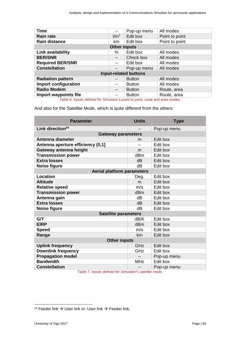
Analysis, design and implementation of a Communications Simulator for aeronautic applications
University of Vigo 2017 Page | 69
Time -- Pop-up menu All modes
Rain rate l/m2 Edit box Point to point
Rain distance km Edit box Point to point
Other inputs
Link availability % Edit box All modes
BER/SNR -- Check box All modes
Required BER/SNR -- Edit box All modes
Constellation -- Pop-up menu All modes
Input-related buttons
Radiation pattern -- Button All modes
Import configuration -- Button All modes
Radio Modem -- Button Route, area
Import waypoints file -- Button Route, area Table 6. Inputs defined for Simulator’s point to point, route and area modes.
And also for the Satellite Mode, which is quite different from the others:
Parameter Units Type
Link direction24 -- Pop-up menu
Gateway parameters
Antenna diameter m Edit box
Antenna aperture efficiency (0,1] -- Edit box
Gateway antenna height m Edit box
Transmission power dBm Edit box
Extra losses dB Edit box
Noise figure dB Edit box
Aerial platform parameters
Location Deg. Edit box
Altitude m Edit box
Relative speed m/s Edit box
Transmission power dBm Edit box
Antenna gain dB Edit box
Extra losses dB Edit box
Noise figure dB Edit box
Satellite parameters
G/T dB/K Edit box
EIRP dBm Edit box
Speed m/s Edit box
Range km Edit box
Other inputs
Uplink frequency GHz Edit box
Downlink frequency GHz Edit box
Propagation model -- Pop-up menu
Bandwidth MHz Edit box
Constellation -- Pop-up menu Table 7. Inputs defined for Simulator's satellite mode.
24 Feeder link User link or: User link Feeder link.
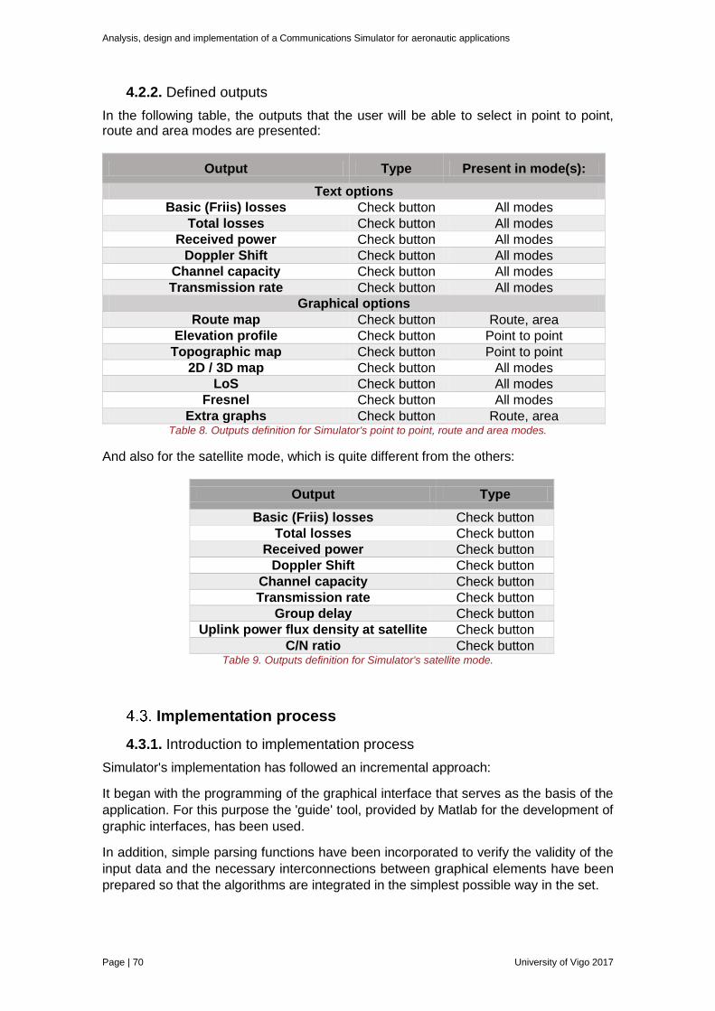
Analysis, design and implementation of a Communications Simulator for aeronautic applications
Page | 70 University of Vigo 2017
4.2.2. Defined outputs
In the following table, the outputs that the user will be able to select in point to point, route and area modes are presented:
Output Type Present in mode(s):
Text options
Basic (Friis) losses Check button All modes
Total losses Check button All modes
Received power Check button All modes
Doppler Shift Check button All modes
Channel capacity Check button All modes
Transmission rate Check button All modes
Graphical options
Route map Check button Route, area
Elevation profile Check button Point to point
Topographic map Check button Point to point
2D / 3D map Check button All modes
LoS Check button All modes
Fresnel Check button All modes
Extra graphs Check button Route, area Table 8. Outputs definition for Simulator's point to point, route and area modes.
And also for the satellite mode, which is quite different from the others:
Output Type
Basic (Friis) losses Check button
Total losses Check button
Received power Check button
Doppler Shift Check button
Channel capacity Check button
Transmission rate Check button
Group delay Check button
Uplink power flux density at satellite Check button
C/N ratio Check button Table 9. Outputs definition for Simulator's satellite mode.
Implementation process
4.3.1. Introduction to implementation process
Simulator's implementation has followed an incremental approach:
It began with the programming of the graphical interface that serves as the basis of the
application. For this purpose the 'guide' tool, provided by Matlab for the development of
graphic interfaces, has been used.
In addition, simple parsing functions have been incorporated to verify the validity of the
input data and the necessary interconnections between graphical elements have been
prepared so that the algorithms are integrated in the simplest possible way in the set.
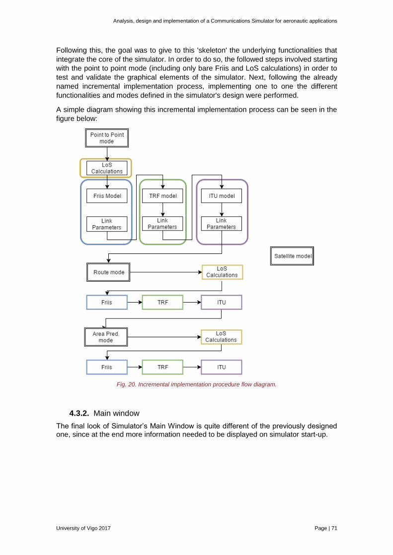
Analysis, design and implementation of a Communications Simulator for aeronautic applications
University of Vigo 2017 Page | 71
Following this, the goal was to give to this 'skeleton' the underlying functionalities that
integrate the core of the simulator. In order to do so, the followed steps involved starting
with the point to point mode (including only bare Friis and LoS calculations) in order to
test and validate the graphical elements of the simulator. Next, following the already
named incremental implementation process, implementing one to one the different
functionalities and modes defined in the simulator's design were performed.
A simple diagram showing this incremental implementation process can be seen in the
figure below:
Fig. 20. Incremental implementation procedure flow diagram.
4.3.2. Main window
The final look of Simulator’s Main Window is quite different of the previously designed one, since at the end more information needed to be displayed on simulator start-up.
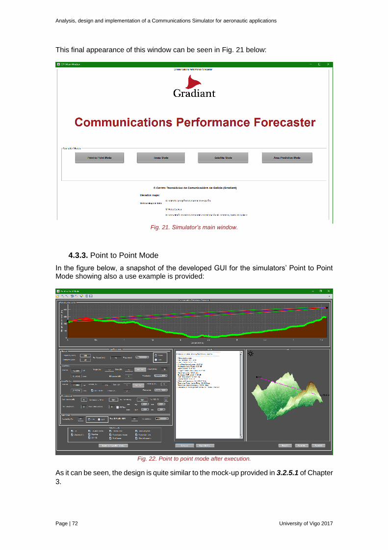
Analysis, design and implementation of a Communications Simulator for aeronautic applications
Page | 72 University of Vigo 2017
This final appearance of this window can be seen in Fig. 21 below:
Fig. 21. Simulator’s main window.
4.3.3. Point to Point Mode
In the figure below, a snapshot of the developed GUI for the simulators’ Point to Point Mode showing also a use example is provided:
Fig. 22. Point to point mode after execution.
As it can be seen, the design is quite similar to the mock-up provided in 3.2.5.1 of Chapter
3.
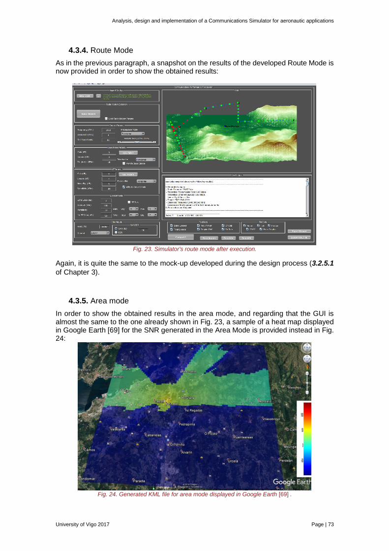
Analysis, design and implementation of a Communications Simulator for aeronautic applications
University of Vigo 2017 Page | 73
4.3.4. Route Mode
As in the previous paragraph, a snapshot on the results of the developed Route Mode is now provided in order to show the obtained results:
Fig. 23. Simulator's route mode after execution.
Again, it is quite the same to the mock-up developed during the design process (3.2.5.1
of Chapter 3).
4.3.5. Area mode
In order to show the obtained results in the area mode, and regarding that the GUI is almost the same to the one already shown in Fig. 23, a sample of a heat map displayed in Google Earth [69] for the SNR generated in the Area Mode is provided instead in Fig. 24:
Fig. 24. Generated KML file for area mode displayed in Google Earth [69] .
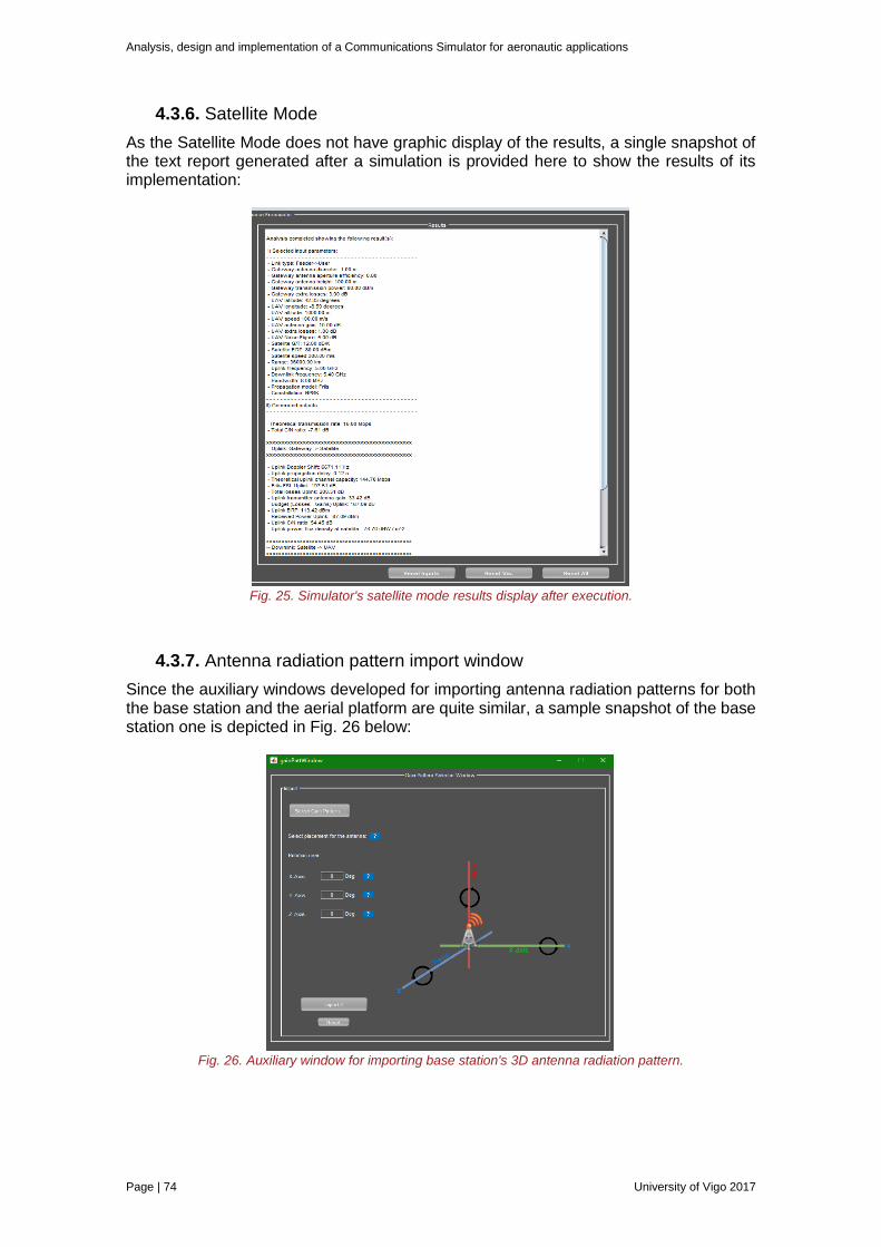
Analysis, design and implementation of a Communications Simulator for aeronautic applications
Page | 74 University of Vigo 2017
4.3.6. Satellite Mode
As the Satellite Mode does not have graphic display of the results, a single snapshot of the text report generated after a simulation is provided here to show the results of its implementation:
Fig. 25. Simulator's satellite mode results display after execution.
4.3.7. Antenna radiation pattern import window
Since the auxiliary windows developed for importing antenna radiation patterns for both the base station and the aerial platform are quite similar, a sample snapshot of the base station one is depicted in Fig. 26 below:
Fig. 26. Auxiliary window for importing base station's 3D antenna radiation pattern.
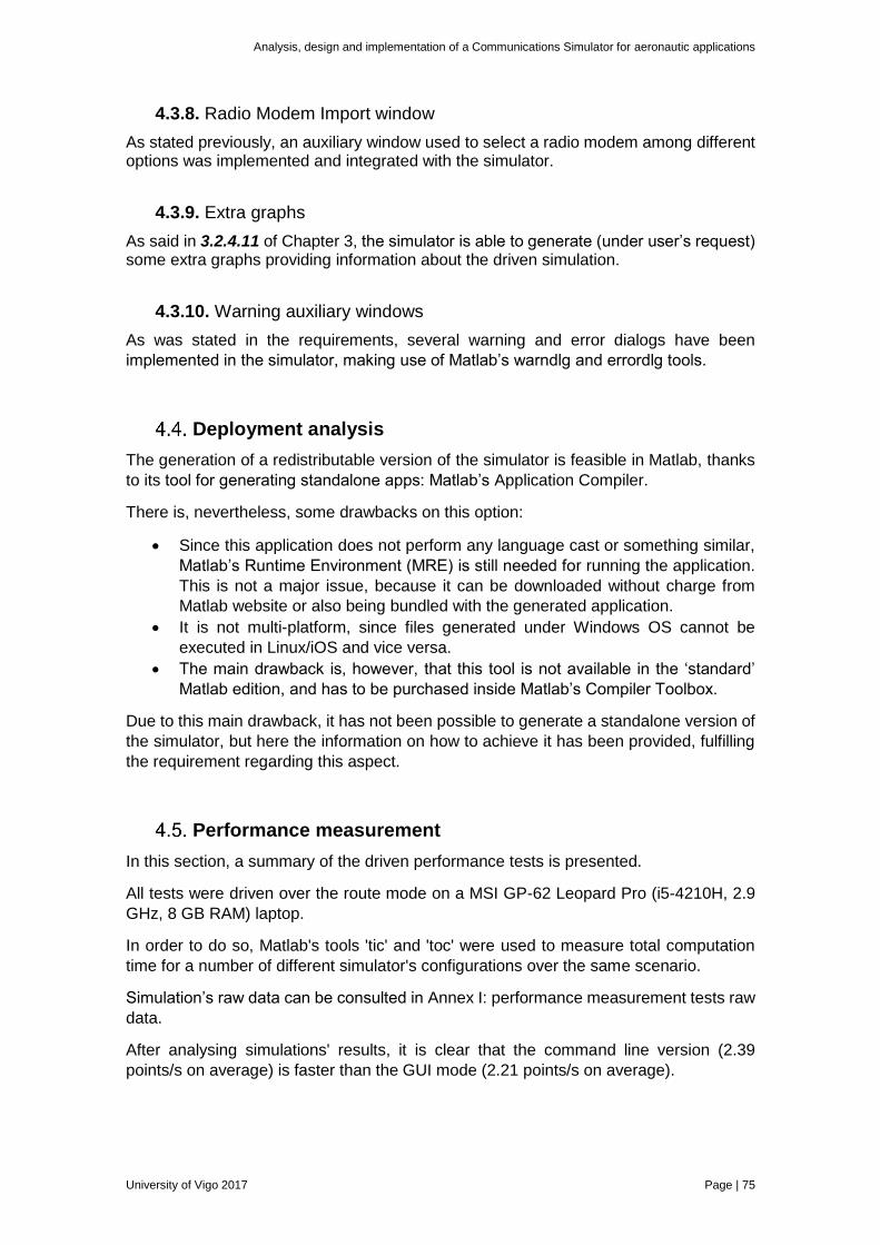
Analysis, design and implementation of a Communications Simulator for aeronautic applications
University of Vigo 2017 Page | 75
4.3.8. Radio Modem Import window
As stated previously, an auxiliary window used to select a radio modem among different options was implemented and integrated with the simulator.
4.3.9. Extra graphs
As said in 3.2.4.11 of Chapter 3, the simulator is able to generate (under user’s request) some extra graphs providing information about the driven simulation.
4.3.10. Warning auxiliary windows
As was stated in the requirements, several warning and error dialogs have been
implemented in the simulator, making use of Matlab’s warndlg and errordlg tools.
Deployment analysis
The generation of a redistributable version of the simulator is feasible in Matlab, thanks
to its tool for generating standalone apps: Matlab’s Application Compiler.
There is, nevertheless, some drawbacks on this option:
Since this application does not perform any language cast or something similar,
Matlab’s Runtime Environment (MRE) is still needed for running the application.
This is not a major issue, because it can be downloaded without charge from
Matlab website or also being bundled with the generated application.
It is not multi-platform, since files generated under Windows OS cannot be
executed in Linux/iOS and vice versa.
The main drawback is, however, that this tool is not available in the ‘standard’
Matlab edition, and has to be purchased inside Matlab’s Compiler Toolbox.
Due to this main drawback, it has not been possible to generate a standalone version of
the simulator, but here the information on how to achieve it has been provided, fulfilling
the requirement regarding this aspect.
Performance measurement
In this section, a summary of the driven performance tests is presented.
All tests were driven over the route mode on a MSI GP-62 Leopard Pro (i5-4210H, 2.9
GHz, 8 GB RAM) laptop.
In order to do so, Matlab's tools 'tic' and 'toc' were used to measure total computation
time for a number of different simulator's configurations over the same scenario.
Simulation’s raw data can be consulted in Annex I: performance measurement tests raw
data.
After analysing simulations' results, it is clear that the command line version (2.39
points/s on average) is faster than the GUI mode (2.21 points/s on average).
Analysis, design and implementation of a Communications Simulator for aeronautic applications
Page | 76 University of Vigo 2017
It should be noted here that time measurements have been made exclusively over
computation's functions, leaving without measure the needed time to represent the
generated information.
In the case of considering extra attenuation due to real time rain (querying to MeteoSix
server) it is observed that the efficiency falls in some cases noticeably, but on average
not more than 0.04 points/s.
However it has to be noted that this is a first implementation of the software in which not
all the possible care when programming has been taken, sacrificing efficiency to
development’s ease. Future versions of the software, which may include migrations to
other languages, could achieve greater efficiencies, which have already been improved
from the initial 1.75 points/s (in a previous development version not covered in the
performance study).
Implementation testing and verification
In this section, the followed testing methods are presented.
While undergoing its implementation, many of its components have been properly tested
and validated prior to adding them to Simulator's core .The elements tested
independently was:
Graphical interface connections.
DTM data loading.
Propagation models' sub routines.
Propagation models.
Output parameters coherence validation.
Meteorological information querying.
Data import functions.
Data display functions.
Output generation functions.
Input parsing functions.
Antenna radiation pattern gain computations.
Event handling (user actions, errors, warnings…).
Warning and error display checks.
After finishing application's implementation, several tests were conducted over to ensure
its proper operation. The main way to perform tests was conducted in the way below:
1. A number of mission's routes were defined in MP.
2. Several sets of input parameters (with different operational frequencies,
bandwidth, gains/antenna radiation patterns, availability percentages...) was set
in different external configuration files.
3. Test executions were conducted combining waypoints' files and configuration's
files available.
Although no field measurements were performed to validate simulations' results, the
underlying objective was to test the coherence of the performed estimations (for
example: ‘ITU’s propagation model should not provide lesser attenuation than Friis one’
or: ‘the heat map in in the generated KML shall not leave uncovered areas at mission
site’) and identify bugs to be tracked and fixed.
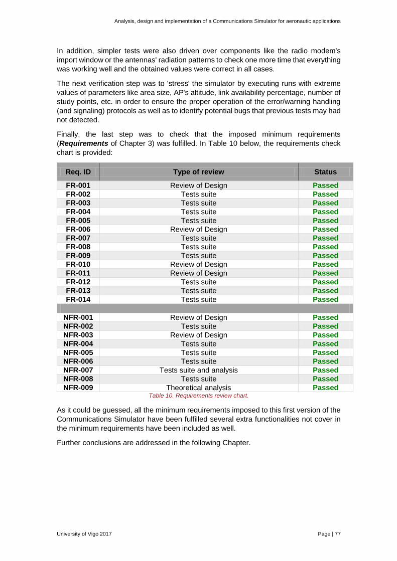
Analysis, design and implementation of a Communications Simulator for aeronautic applications
University of Vigo 2017 Page | 77
In addition, simpler tests were also driven over components like the radio modem's
import window or the antennas' radiation patterns to check one more time that everything
was working well and the obtained values were correct in all cases.
The next verification step was to 'stress' the simulator by executing runs with extreme
values of parameters like area size, AP's altitude, link availability percentage, number of
study points, etc. in order to ensure the proper operation of the error/warning handling
(and signaling) protocols as well as to identify potential bugs that previous tests may had
not detected.
Finally, the last step was to check that the imposed minimum requirements
(Requirements of Chapter 3) was fulfilled. In Table 10 below, the requirements check
chart is provided:
Req. ID Type of review Status
FR-001 Review of Design Passed
FR-002 Tests suite Passed
FR-003 Tests suite Passed
FR-004 Tests suite Passed
FR-005 Tests suite Passed
FR-006 Review of Design Passed
FR-007 Tests suite Passed
FR-008 Tests suite Passed
FR-009 Tests suite Passed
FR-010 Review of Design Passed
FR-011 Review of Design Passed
FR-012 Tests suite Passed
FR-013 Tests suite Passed
FR-014 Tests suite Passed
NFR-001 Review of Design Passed
NFR-002 Tests suite Passed
NFR-003 Review of Design Passed
NFR-004 Tests suite Passed
NFR-005 Tests suite Passed
NFR-006 Tests suite Passed
NFR-007 Tests suite and analysis Passed
NFR-008 Tests suite Passed
NFR-009 Theoretical analysis Passed Table 10. Requirements review chart.
As it could be guessed, all the minimum requirements imposed to this first version of the
Communications Simulator have been fulfilled several extra functionalities not cover in
the minimum requirements have been included as well.
Further conclusions are addressed in the following Chapter.

Analysis, design and implementation of a Communications Simulator for aeronautic applications
University of Vigo 2017 Page | 79
5. Conclusions
This project has required to deal with different technical issues such as: radio
propagation models, Digital Terrain Models, meteorological data acquisition, geography
and so on. Its development led to the following conclusions:
There are many commercially available software tools which model radio
propagation. Some of them are suitable to be used in aeronautic
applications.
The most common results provided by these kind of tools are graphical
displays of information and data reports. Among the modelled parameters are
the Signal to Noise Ratio and the sensitivity. Many of them make use of Digital
Terrain Models together with radio propagation models to perform its
estimations.
There are many different radio propagation models available, several
standardized by organizations like ITU. Each one takes into account a number
of different propagation mechanisms. Depending on how results are obtained,
they can be divided in deterministic, empirical, and stochastic models.
There is no clear difference between aerial and terrestrial channel. Thus, the
relevant parameters to consider the use of a radio propagation model in
aeronautic applications are frequency, altitude and range for which they are
intended.
There are different Digital Terrain Models with different degrees of
resolution available. In addition, some consider height of terrain’s surface
objects as well.
Interferences are a complex impairment to communication data link
performance that require a deep characterization in order to be modelled.
Rain attenuation on radio propagation has to be considered for frequencies
above 5 GHz.
To take into account antennas’ radiation patterns has a huge impact in the
estimated signal level at the receiver.
The following scenarios have been identified as significant ones where to
forecast communication data link performance: point to point link, route, area
and satellite link.
Taking into account the State of the Art, the following parameters have been
identified as useful to model communication data link performance: Link
Budget, LoS conditions, Fresnel Clearance, Signal to Noise Ratio, Sensitivity,
Doppler Shift, Channel Capacity and Transmission Rate.

Analysis, design and implementation of a Communications Simulator for aeronautic applications
Page | 80 University of Vigo 2017
The simulator has been implemented in Matlab due to its flexibility,
capabilities and development ease. Its integrated ‘guide’ tool has been used
to generate Simulator’s Graphical User Interface as well.
Functional and performance tests have been performed to check the
coherence of the performed estimations and to identify bugs to be tracked and
fixed.
In the following Chapter, last of this document, several future lines of development
which have already been identified are addressed to complement these drawn
conclusions, including both some upgrades over existent functionalities and new
features.
Analysis, design and implementation of a Communications Simulator for aeronautic applications
University of Vigo 2017 Page | 81
6. Future lines of development
The considered future lines of development can be divided into two main blocks:
developing new features and upgrade existing ones, including corrections, refactoring
and optimisation.
Related with this two blocks, perform a set of field tests in order to compare
Simulator’s estimations with real measurements might be one of the best actions to
take in the future. This would provide a way to determine the reliability of the Simulator
and so identify the need of adjusting different elements of it (ranging from propagation
models to antennas' gains calculations among others).
Upgrades over existing features
Among the existing features, further development could be performed in order to
provide improvements in functionality and added value to users:
Aerial platform's flight dynamics might be taken into account since the AP
perform turns in pitch and roll which can affect to the gain value of the antennas
(the angles of view change with every turn). This would enable to model in a more
realistic way the effects of the antennas, which not irradiate the same amount of
signal in all directions.
Porting the application to another language / platform might improve its
performance, since there are several available options which are more powerful
(in terms of performance) and easier to deploy to end user than Matlab. A
discussion regarding the different considered programming languages is already
available in 4.1 although it might be expanded in the future.
Regarding functionalities which have a range of possible upgrades, more
propagation models might be explored in order to be added to Simulator’s
Satellite Mode, enhancing its current capabilities.
Having in mind 2.3.3, to evaluate in the future the possibility of take into account
surface objects' height (trees, buildings...) might be interesting. In case of
feasibility, a DEM could be implemented or a DSM could be added to the already
available DTM, which would even better because that would let the user choose
whether to consider surface objects' height or not.
The effect of input parameters like conductivity or permittivity (and perhaps
some others) might be evaluated and, based on the obtained results remove
them from the inputs' list, relieving the user to specify them and simplifying the
operation of the simulator. Of course, the parameters still would be considered,
but in a transparent way to end user (for example, getting their values from
several internal lists which would provide values for different locations).
Relying on external services such as the IGN WCS server [53] or the MeteoSix
[62] server is a potential source of issues. Servers' maintenance shutdowns,
changes in the way the data are accessed and failures due to overload may led
Analysis, design and implementation of a Communications Simulator for aeronautic applications
Page | 82 University of Vigo 2017
into not delivering the needed reliability level, depending on the final usage of the
simulator.
Since these impairments are expected to happen in some queries to servers
without previous notice, the approach to resolve this issue might be to search
again in order to find better conditioned servers or to develop a dedicated
server for storing application data.
New features
6.2.1. Functional Features
Regarding new functionalities, the following ones might increase the number of use cases for which the Simulator is suitable to be used:
Increase the number of radio propagation models available might enable the
Simulator to increase the number of use cases for which is intended. Adding more
radio propagation models would lead to an increment of usability, because of the
wider number of scenarios and environments which could be modelled. Taken to
the limit, a high number of models might be implemented being each one focused
on a particular scenario.
Related with the last paragraph, the influence of more meteorological
phenomena in communications might be evaluated and modelled (if found
non-negligible) in order to provide attenuation values and enhance the way these
are displayed in the GUI. This development line is open also to find environmental
conditions that could potentially affect a radio signal and to implement models
which enable the Simulator to forecast the identified ones.
Furthermore, it might to be considered the possibility of taking into account
terrain's kind and / or usage and autonomously determine some environment
and / or transmission parameters (conductivity, refractivity, extra losses...)
derived from it. This would be conditioned to a study which should be carried out
regarding the trade-off between complexity and degree of improvement over
estimations.
Additionally, as covered in the state of-the-art analysis, it could be taken into
account the effect of interferences over a communications' link, perhaps using
the considerations in 2.4.3 as a starting point and then further developing them
until a more realistic interference modelling process was achieved.
6.2.2. Operational Features
Thinking now in operational features, or more likely, underlying features transparent
to application's users, several steps might be taken in the future:
First of all, (and in a related way with application migration to another language /
platform) enable multi-threading computation would lead in a huge increment
of performance, since computation time would be reduced.
Analysis, design and implementation of a Communications Simulator for aeronautic applications
University of Vigo 2017 Page | 83
Moreover, considering the possibility of building posterior Simulator's versions in
a cloud based architecture could increase both its performance and its
protection against piracy and unauthorized use as well as decrease development
ease (if, for example a cross-platform application has to be developed), thus this
option should be studied in the future.
Last but not least, as has been already commented in 2.3.3, to integrate the
developed functionalities with an already existent GIS or mission planner
would enable end user to operate an already optimised graphical tool, enabling
easier operation of the simulator25 and avoiding of the implementation and
optimisation of these tools by project's developers.
25 For example, enabling to specify waypoints, base station location, mission area…in an easier way (graphically dragging and dropping the mouse) than the actual one (through files).

Analysis, design and implementation of a Communications Simulator for aeronautic applications
University of Vigo 2017 Page | 85
7. References
[1] “PFPS: Portable Flight Planning System.” [Online]. Available: https://www.falconview.org/trac/FalconView/wiki/PFPS.
[2] Global Security, “Mission Planning System (MPS),” Air Force Programs, 2010.
[3] Defense technical Information Center, “Mission Description and Budget Item Justification (for MPS),” 2012.
[4] Boeing, “MISSION PLANNING SYSTEMS: Delivering a Full Range of Integrated Planning Services,” Commercial Brochure. [Online]. Available: http://www.boeing.com/assets/pdf/defense-space/support/training/product_cards/MissionPlanning.pdf.
[5] Leica Geosystems, “Leica MissionPro Flight Planning Software,” MissionPro Product Brochure. [Online]. Available: http://leica-geosystems.com/products/airborne-systems/software/leica-missionpro.
[6] “Hexagon AB – Global provider of information technologies for industrial and geospatial applications | Hexagon.” [Online]. Available: http://hexagon.com/.
[7] Telos, “SE7EN: Mission Planner,” Product Brochure. [Online]. Available: https://www.telos.com/wp-content/uploads/2015/10/Telos-SE7EN-Mission-Planner-brochure.pdf.
[8] UgCS, “Mission planner,” Product brochure. [Online]. Available: https://www.ugcs.com/en/features/mission-planner-and-drone-control.
[9] UgCS, “UgCS SDK.” [Online]. Available: https://www.ugcs.com/en/page/sdk.
[10] Skysense, “Skysense Planner.” [Online]. Available: http://www.skysense.co/planner-launch.
[11] M. Oborne, “Mission Planner documentation.” [Online]. Available: http://ardupilot.org/planner/.
[12] John Magliacane, “SPLAT! A Terrestrial RF Path Analysis Application For Linux/Unix.” [Online]. Available: http://www.qsl.net/kd2bd/splat.html.
[13] Remcom, “InSite: Wireless EM Propagation Software.” [Online]. Available: https://www.remcom.com/wireless-insite-em-propagation-software/.
[14] Forsk, “Atoll - Radio planning software.” [Online]. Available: http://www.forsk.com/atoll/.
[15] RadioSoft, “Comstudy 2.2: Radio Propagation Software.” [Online]. Available: http://rad.radiosoft.com/.
[16] EDX Wireless, “SignalPro.” [Online]. Available: http://edx.com/products/edx-signalpro/.
[17] Contract Telecomunication Engineering, “Pathloss 5 - Microwave Radio Link Design and Planning Software.” [Online]. Available: http://www.pathloss.com/index.php#!p5prod.
[18] V-Soft Communications, “PlotPath – Broadcast Engineering, Signal Propagation, and FCC Allocation Software.” [Online]. Available: http://www.v-soft.com/plotpath.
[19] V-Soft Communications, “Probe 4: RF Propagation Prediction Software,” Product Brochure. [Online]. Available: http://www.v-soft.com/wp-
Analysis, design and implementation of a Communications Simulator for aeronautic applications
Page | 86 University of Vigo 2017
content/uploads/2011/11/Probe4_Brochure.pdf.
[20] V-Soft Communications, “Terrain-3D – Broadcast Engineering, Signal Propagation, and FCC Allocation Software.” [Online]. Available: http://www.v-soft.com/terrain-3d.
[21] Siradel, “Volcano: Best-in-class radio propagation models.” [Online]. Available: https://www.siradel.com/software/connectivity/volcano-software/.
[22] Roger Coudé, “Radio Mobile Online - Online RF propagation simulation software.” [Online]. Available: http://radiomobileonline.pe1mew.nl/?About_Radio_Mobile_Online.
[23] Farrant Consulting, “Cloud RF: Open source propagation modelling cloud tool.” [Online]. Available: https://cloudrf.com/open source.
[24] AGI, “STK - software to model, analyze and visualize space, defense and intelligence systems.” [Online]. Available: http://www.agi.com/solutions/main.aspx/id/uav-and-aircraft-missions.
[25] AGI, “STK - STK Communications & STK Radar.” [Online]. Available: http://help.agi.com/stk/index.htm#comm/CommRadar.htm%3FTocPath%3DSTK%7CAdd-on%2520Modules%7CCommunications%2520%2526%2520Radar%7C_____0.
[26] Integrasys, “AeroTrackCOM.” [Online]. Available: http://www.integrasys-space.com/#!services/c9kl.
[27] Insitu, “Insitu Common Open Mission Management Command and Control (ICOMC2).” [Online]. Available: https://insitu.com/information-delivery/command-and-control/icomc2.
[28] Insitu, “ICOMC2 - RFLA Plug-in.” [Online]. Available: https://insitu.com/information delivery/command-and-control/icomc2/icomc2-rfla.
[29] G. Sati and S. Singh, “A REVIEW ON OUTDOOR PROPAGATION MODELS IN RADIO COMMUNICATION,” Int. J. Comput. Eng. Sci. ©IJCES ISSN, vol. 4, no. 2, pp. 2231–6590, 2014.
[30] ITU-R, “A general purpose wide-range terrestrial propagation model in the frequency range 30 MHz to 50 GHz,” Recomm. ITU-R p.2001-2, 2015.
[31] ITU-R, “Prediction of path attenuation on links between an airborne platform and Space and between an airborne platform and the surface of the Earth,” Recomm. ITU-R P.2041-0, 2013.
[32] ITU-R, “Propagation curves for aeronautical mobile and radionavigation services using the VHF, UHF and SHF bands,” Recomm. ITU-R P.528-3, 2012.
[33] ITU-R, “Defining propagation model for Recommendation ITU-R P.528-3,” 2015.
[34] ITU-R, “Calculation of Free-Space Attenuation,” Recomm. ITU-R P.525-2, vol. 1, no. 2, pp. 2–4, 1994.
[35] ITU-R, “Propagation data and prediction methods required for the design of Earth-space telecommunication systems,” Recomm. ITU-R P.618-12, 2015.
[36] ITU-R, “Propagation data required for the design of Earth-space land mobile telecommunication systems,” Recomm. ITU-R P.681-9, pp. 681–9, 2016.
[37] ITU-R, “Propagation data required for the design of Earth-space aeronautical
Analysis, design and implementation of a Communications Simulator for aeronautic applications
University of Vigo 2017 Page | 87
mobile telecommunication systems,” Recomm. ITU-R P.682-3 , 2012.
[38] P. L. Longley, A G., and Rice, “Prediction of Tropospheric Radio Transmission Loss Over Irregular Terrain; A Computer Method,” ESSA Tech. Rep., vol. ERL 79-IT, 1968.
[39] D. E. and W. Kuebler, “TIREM/SEM HANDBOOK,” in Electromagnetic Compatibility Analysis Center, no. MARCH 1994, 1986.
[40] AGI, “STK - Using the Terrain Integrated Rough Earth Model (TIREM).” [Online]. Available: http://help.agi.com/stk/index.htm#training/tirem.htm.
[41] Y. S. Meng and Y. H. Lee, “Measurements and Characterizations of Air-to-Ground Channel Over Sea Surface at C-Band With Low Airborne Altitudes,” IEEE Trans. Veh. Technol., vol. 60, no. 4, pp. 1943–1948, May 2011.
[42] D. Vanhoenacker-Janvier, P. Bouchard, L. E. Bråten, V. Fabbro, C. Kourogiorgas, and D. Rogers, “Channel models for aeronautical and low elevation radio links,” Antennas and Propagation (EuCAP), 2013 7th European Conference on. IEEE, pp. 3184–3186, 2013.
[43] A. Al-Hourani, S. Kandeepan, and A. Jamalipour, “Modeling air-to-ground path loss for low altitude platforms in urban environments,” in 2014 IEEE Global Communications Conference, 2014, pp. 2898–2904.
[44] M. Simunek, F. P. Fontan, and P. Pechac, “The UAV Low Elevation Propagation Channel in Urban Areas: Statistical Analysis and Time-Series Generator,” IEEE Trans. Antennas Propag., vol. 61, no. 7, pp. 3850–3858, Jul. 2013.
[45] J. Zelený, F. Pérez-Fontán, and P. Pechač, “Initial Results from a measurement campaign for low elevation angle links in different environments,” 2015 9th European Conference on Antennas and Propagation (EuCAP). IEEE, pp. 1–4, 2015.
[46] P. Hoeher and E. Haas, “Aeronautical channel modeling at VHF-band,” in Gateway to 21st Century Communications Village. VTC 1999-Fall. IEEE VTS 50th Vehicular Technology Conference (Cat. No.99CH36324), 1999, vol. 4, pp. 1961–1966 vol.4.
[47] E. Haas, “Aeronautical channel modeling,” IEEE Trans. Veh. Technol., vol. 51, no. 2, pp. 254–264, Mar. 2002.
[48] Georgia Tech Research Institute, “FalconView,” FalconView Wiki. [Online]. Available: https://www.falconview.org/trac/FalconView.
[49] NASA, “NASA World Wind Server Homepage.” [Online]. Available: https://worldwind.arc.nasa.gov/.
[50] Google, “Google Maps API | Google Developers.” [Online]. Available: https://developers.google.com/maps/?hl=es-419.
[51] G. de E. Ministerio de Fomento, “Instituto Geográfico Nacional.” [Online]. Available: http://www.ign.es/ign/main/index.do.
[52] G. de E. Misterio de Fomento, “Infraestructura de Datos Espaciales Española - Estándar de interfaz.”
[53] G. de E. Ministerio de Fomento, “Instituto Geográfico Nacional - Infraestructura de datos espaciales.” [Online]. Available: http://www.ign.es/web/ign/portal/ide-area-nodo-ide-ign.
Analysis, design and implementation of a Communications Simulator for aeronautic applications
Page | 88 University of Vigo 2017
[54] ITU-R, “Prediction procedure for the evaluation of interference between stations on the surface of the Earth at frequencies above about 0.1 GHz,” Rec. ITU-R P.452-16 , 2015.
[55] Prapun Suksompong, “2.2 Co-Channel Interference,” ECS455.
[56] Danny W.H. Tham, “Carrier to Interference (C/I ratio) Calculations,” ITU Reg. Radiocommun. Semin. Asia, 2014.
[57] Amphenol Antennas, “Atenna Pattern Files extensions.” [Online]. Available: http://www.amphenol-antennas.com/Pattern-Files.aspx.
[58] Sinclair Technologies, “Antenna Pattern Files.” [Online]. Available: http://www.sinctech.com/resources/technical-documents/antenna-pattern-files/.
[59] Matlab, “Antenna Toolbox.” [Online]. Available: https://es.mathworks.com/products/antenna.html.
[60] Radio Frequency Systems, “Microwave Antenna Patterns.” [Online]. Available: http://www.rfsworld.com/microwave-antenna-patterns,81,1.html.
[61] ITU-R, “Specific attenuation model for rain for use in prediction methods,” Rec. ITU-R p.838-3, 2005.
[62] MeteoGalicia, “API do MeteoSIX v3.” [Online]. Available: http://servizos.meteogalicia.gal/api_manual/gl/index.html.
[63] SatSig, “Satellite Link Budget Calculator.” [Online]. Available: http://www.satsig.net/linkbugt.htm.
[64] IDC Technologies, “3.11 The Uplink,” Eng. course.
[65] IDC Technologies, “Fresnel Zones,” Eng. course.
[66] T. S. Duffy, “Section 22: the Doppler effect for EM Waves,” in Electromagnetic Propagation, 2010.
[67] Univerity of St. Andrews [GB], “Shannon’s Equation and Channel Capacity.” [Online]. Available: https://www.st-andrews.ac.uk/~www_pa/Scots_Guide/iandm/part8/page1.html. [Accessed: 21-Apr-2017].
[68] J. (John) Dunlop and D. G. (D. G. Smith, Telecommunications engineering. Stanley Thornes, 1998.
[69] “Keyhole Markup Language | Google Developers.” [Online]. Available: https://developers.google.com/kml/?csw=1. [Accessed: 04-Jun-2017].
[70] F.Hugo Ramírez Leyva, “Robótica: Modelado de cinemática de robots,” UTM.
[71] ITU-R, “Propagation data and prdiction methods required for the design of terrestrial line of sight systems,” Rec. ITU-R p.530-16.
[72] ArcGIS Community, “Python for ArcGIS | ArcGIS Resource Center.” [Online]. Available: http://resources.arcgis.com/es/communities/python/.
[73] QGIS, “Building a Python extension — QGIS Tutorials and Tips.” [Online]. Available: https://www.qgistutorials.com/es/docs/building_a_python_plugin.html.
Analysis, design and implementation of a Communications Simulator for aeronautic applications
University of Vigo 2017 Page | 89
Annexes

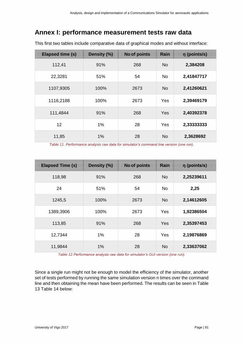
Analysis, design and implementation of a Communications Simulator for aeronautic applications
University of Vigo 2017 Page | 91
Annex I: performance measurement tests raw data
This first two tables include comparative data of graphical modes and without interface:
Elapsed time (s) Density (%) No of points Rain η (points/s)
112,41 91% 268 No 2,384208
22,3281 51% 54 No 2,41847717
1107,9305 100% 2673 No 2,41260621
1116,2188 100% 2673 Yes 2,39469179
111,4844 91% 268 Yes 2,40392378
12 1% 28 Yes 2,33333333
11,85 1% 28 No 2,3628692
Table 11. Performance analysis raw data for simulator’s command line version (one run).
Elapsed Time (s) Density (%) No of points Rain η (points/s)
118,98 91% 268 No 2,25239611
24 51% 54 No 2,25
1245,5 100% 2673 No 2,14612605
1389,3906 100% 2673 Yes 1,92386504
113,85 91% 268 Yes 2,35397453
12,7344 1% 28 Yes 2,19876869
11,9844 1% 28 No 2,33637062
Table 12.Performance analysis raw data for simulator’s GUI version (one run).
Since a single run might not be enough to model the efficiency of the simulator, another
set of tests performed by running the same simulation version n times over the command
line and then obtaining the mean have been performed. The results can be seen in Table
13 Table 14 below:
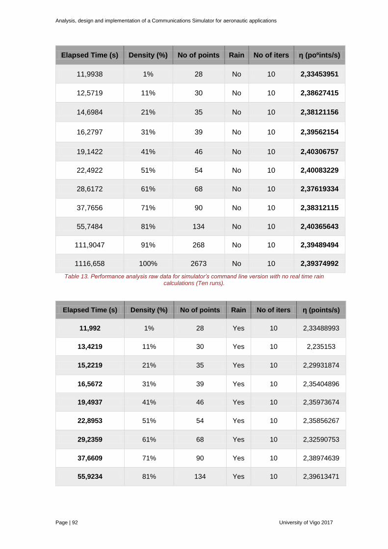
Analysis, design and implementation of a Communications Simulator for aeronautic applications
Page | 92 University of Vigo 2017
Elapsed Time (s) Density (%) No of points Rain No of iters η (poºints/s)
11,9938 1% 28 No 10 2,33453951
12,5719 11% 30 No 10 2,38627415
14,6984 21% 35 No 10 2,38121156
16,2797 31% 39 No 10 2,39562154
19,1422 41% 46 No 10 2,40306757
22,4922 51% 54 No 10 2,40083229
28,6172 61% 68 No 10 2,37619334
37,7656 71% 90 No 10 2,38312115
55,7484 81% 134 No 10 2,40365643
111,9047 91% 268 No 10 2,39489494
1116,658 100% 2673 No 10 2,39374992
Table 13. Performance analysis raw data for simulator’s command line version with no real time rain calculations (Ten runs).
Elapsed Time (s) Density (%) No of points Rain No of iters η (points/s)
11,992 1% 28 Yes 10 2,33488993
13,4219 11% 30 Yes 10 2,235153
15,2219 21% 35 Yes 10 2,29931874
16,5672 31% 39 Yes 10 2,35404896
19,4937 41% 46 Yes 10 2,35973674
22,8953 51% 54 Yes 10 2,35856267
29,2359 61% 68 Yes 10 2,32590753
37,6609 71% 90 Yes 10 2,38974639
55,9234 81% 134 Yes 10 2,39613471

Analysis, design and implementation of a Communications Simulator for aeronautic applications
University of Vigo 2017 Page | 93
110,9875 91% 268 Yes 10 2,41468634
1128,35 100% 2673 Yes 10 2,36894581
Table 14. Performance analysis raw data for simulator’s command line version with real time rain calculations (Ten runs).