Analysis and Visualization of Electromagnetic Situation

Analysis and Visualization of Electromagnetic Situation Based on Raster Database

Hanyan Huang*, Mingshan Shao, Hua Zhang and Yulan Chen Wuhan Mechanical Technology College, Wuhan, Hubei, China, 430075

*Corresponding author

Abstract—It is with great significance to improve the speed of analysis and visualization of electromagnetic situation. However, The calculation amount of wave propagation involving numbers of radiation sources to form the electromagnetic situation is very large, and directly calculation is time-consuming. In this paper, the raster database is introduced into the calculation and storage of electromagnetic situation. Then, the corresponding isoline tracing algorithm for regular raster structure is given, as well as the isoline smoothing and filling algorithm. At last, the calculation efficiency of the developed method is compared with the previous method under the same electromagnetic environment. In the developed system the calculation time can be shortened from more than 17 hours to 20 minutes, and 100 radiation sources in the application scenario can be calculated and visualized in 1 minute. All of this show that the electromagnetic situation raster database can significantly improve the system running speed and the data application efficiency.

Keywords-electromagnetic situation; raster database; isoline tracing; visualization; electromagnetic field intensity

I. INTRODUCTION

Electromagnetic environment perception is the foundation of all actions in electronic warfare, and it is also the key to gain advantages in fighting for the electromagnetic control [1]. Visualization is an indispensable man-machine communication step in the process of electromagnetic situational perception. Based on the 3-layers electromagnetic situational perception model developed by Endsley including situational factors of extraction, situation understanding and situation forecast, the visualization layer is added by [2]. Situational analysis and visualization functions are included in some spectrum management tool, such as WRAP developed by LuBo in Sweden, the U.S. military’s SPECTRUM XXI and CJSMPT, AREPS[3][4] etc. The functions of analysis and visualization of the calculation results, statistical and display the situation occupation by 2-dimensions are partly included in these tools. The domestic research about electromagnetic situational perception and visualization is mainly around adding maps, improving the speed and efficiency[5][6]. The basic idea is using the wave propagation model considering the factors such as terrain, weather to calculate the electromagnetic field intensity of each discrete point, and then generate the Delaunay triangulation with its node denoting the discrete point coordinates and field intensity value, then lastly generate electromagnetic situation maps by isoline tracing. The

electromagnetic distribution situation, isoline, propagation path, and other forms of electromagnetic environment visualization are implemented in paper [7]. He Jun[8] proposed an improved pushing algorithm to construct the Delaunay triangulation network, and thus improved the generation speed of two-dimensional electromagnetic situation maps. As using GIS map function can simplify the battlefield electromagnetic environment visualization module[9]. In this paper, the raster database is introduced into the calculation of electromagnetic situation to carry forward the visual intuitive of the geographic raster data, at the same time significantly improve the system running speed and the data application efficiency..

II. ELECTROMAGNETIC CALCULATION MODEL AND

CALCULATION EFFICIENCY ANALYSIS

There are three sub-problems need to solve to describe the electromagnetic environment based on radiation source perception: 1) modeling with frequency equipment; 2) wave propagation calculation based on the geographic information system; 3) electromagnetic description model of situational elements.

A. Parameter Model Of Frequency Equipment

According to the radiation and receiving properties of equipment, the numerical model of frequency equipment is built by the following four sub-models, and accordingly can be used to predict the radio waves propagation and interference of equipment: (1) Basic models of frequency equipment, provide the model parameters including the type, name, name of radar/communication or other frequency equipments. Based on that, the model parameters of transmitter, receiver, antenna can be viewed. (2) Transmitter model, provide transmitter model parameters such as transmission power, upper and lower frequency, channel interval and the signal bandwidth. (3) the receiver model: provide the upper and lower receive frequency, channel spacing, sensitivity, signal bandwidth, and many other receiver model parameters. (4) antenna model: provide model parameters of whip antenna, logarithmic cycles and other types of antenna such as frequency, gain, sidelobe ratio, horizontal vertical direction graph data of the antenna. The E-R diagram for equipment model is shown in FIGURE I. The accuracy of electromagnetic environment analysis and visualization depends largely on the accuracy and authenticity of the frequency equipment model. It is necessary to modify the existing antenna model and propagation model according to the

Modeling, Simulation and Optimization Technologies and Applications (MSOTA 2016)

Copyright © 2016, the Authors. Published by Atlantis Press. This is an open access article under the CC BY-NC license (http://creativecommons.org/licenses/by-nc/4.0/).

Advances in Computer Science Research, volume 58

388

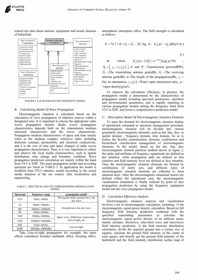
related test data about stations, equipment and actual situation of battlefield.

Parameter relationship of equipment

Main information of

antennaantenna numberantenna nameLower FrequencyUpper frequency gain sidelobe ratio, horizontal direction graph dataVertical direction graph data……

Basic information of

equipment

equipment numberEquipment typeequipment nameMain functionTransceiver categoriesUsing condition mobility remarks……

Main information of

receiver

receiver numberreceiver name upper frequencylower frequency channel spacingsensitivity3dB bandwidth for high frequency20dB bandwidth for high frequency3dB bandwidth for mid frequency20dB bandwidth for mid frequencyNoise figureSignal to noise ratio……

Main information of

Transmitter

Transmittor numberTransmission nametransmission power,Average powerfrequency upperfrequency lower channel interval 3dB bandwidth20dB bandwidth……

FIGURE I. E-R DIAGRAM FOR EQUIPMENT MODEL

B. Calculating Model Of Wave Propagation

Electromagnetic situation is calculated based on the calculation of wave propagation of radiation sources within a designated area. It is important to choose the appropriate radio waves propagation models. Radio waves propagation characteristics depends both on the transmission medium structural characteristic and the waves characteristic. Propagation medium characteristics of space and time mainly refers to the medium complex refractive index including dielectric constant, permeability and electrical conductivity, and it is the root of time and space changes of radio waves propagation characteristics. Thus, it is very important to collect and observe the local media characteristics, such as spatial distribution, time change and boundary condition. Wave propagation prediction calculation are mainly within the band from VLF to EHF. The main propagation model and according spectrum are listed in TABLE I. In application the model is modified from ITU's statistics model according to the actual media situation of the our country after localization and engineering.

TABLE I. SPECTRUM AND ITS CORRESPONDING PROPAGATION MODEL

Spectrum frequency range propagation model

VLF 9kHz -30kHz Waveguide mode, ground wave, the

sky wave

LF 30kHz -300kHz Ground wave, the sky wave MF 300kHz -3000kHz

HF 3MHz-30MHz

VHF 30MHz-300MHz Space wave, diffraction, troposcatter, line of sight, etc UHF 300MHz-3000MHz

SHF 3GHz-30GHz Line-of-sight

EHF 30GHz-100GHz Take Line-of-sight propagation for example, the main

effects considered includes multipath effect, focusing effect,

atmospheric absorption effect. The field strength is calculated as follows:

74.7 20 log ( )t t r s gE P G G d E p A (dBμV/m )

In which 10( ) 2.6 1 log 50dsE p e p ,

g o wA d and tP --Transmission power(dBW),

tG --The transmitting antenna gain(dB), rG --The receiving

antenna gain(dB), d--The length of the propagation(dB), o --

Dry air attenuation, w --Water vapor attenuation ratio, -

-vapor density(g/m3).

To improve the calculation efficiency, in practice, the propagation model is determined by the characteristics of propagation model including spectrum parameters, operation and environmental parameters, and is rapidly matching to various propagation models among the frequency band form VLF to EHF, and forms a comprehensive prediction model.

C. Description Model Of Electromagnetic Situation Elements

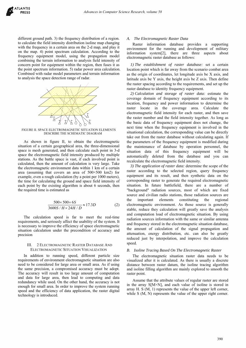
To meet the demand for electromagnetic situation display of operational command or spectrum management personnel, electromagnetic situation will be divided into various granularity electromagnetic elements, such as dot, line, face, or spatial domain , frequency domain, time domain, So as to realize the flexible customization, dynamic combination and hierarchical classification management of electromagnetic elements. In the model, based on the dot, line, face electromagnetic element partition method shown in figure 2, the entity and attributes of frequency equipments are defined as dot situation, while propagation path are defined as line situation and field intensity level are defined as face situation. Then the electromagnetic situation elements are formed by combination of entity sets, and different types of electromagnetic situation elements are collected to form situation layer. After the electromagnetic situational factors are defined within the operational area, the electromagnetic visualization simulation is finally realized by point to face propagation prediction by using the frequency equipment model and the wave propagation model.

D. Calculation Efficiency Analysis

Electromagnetic situation analysis and visualization involves a lot of electromagnetic calculation, including: 1) the electromagnetic signal power density calculation. Based on full frequency field intensity prediction combined with the specified transmitting parameters to calculate the electromagnetic signal power density of an arbitrary point, mainly includes: shortwave, ultra-short wave and microwave field intensity prediction. 2) the field intensity distribution calculation. divide the regional ground into a certain size of squares, calculate the ground field intensity of the center of each square, and thereby get the ground field intensity of the battlefield and the field intensity distribution isoline map of


389

different ground path. 3) the frequency distribution of a region. to calculate the field intensity distribution isoline map changing with the frequency in a certain area on the 2-d map, and play it on the map. 4) point spectrum calculation. According to the frequency equipment model, using the propagation model combining the terrain information to analysis field intensity of concern point for equipment within the region, then fuses it as the point spectrum information. 5) radar power area calculation. Combined with radar model parameters and terrain information to analysis the space detection range of radar.

FIGURE II. SPACE ELECTROMAGNETIC SITUATION ELEMENTS

DESCRIBE THE SCHEMATIC DIAGRAM

As shown in figure II, to obtain the electromagnetic situation of a certain geographical area, the three-dimensional space is mesh generated, and then calculate each point in 3-d space the electromagnetic field intensity produced by multiple stations. As the battle space is vast, if each involved point is calculated, then the amount of calculation is very large. Take the electromagnetic environment data within 1 km of a certain area (assuming that covers an area of 500×500 km2) for example, even a rough calculation (by a point per 1000 meters), the time for calculating the ground and space field intensity of each point by the existing algorithm is about 6 seconds, then the required time is estimated as

500 500 617.3

3600 / 24 /

SD

S H H D

The calculation speed is far to meet the real-time requirements, and seriously affect the usability of the system. It is necessary to improve the efficiency of space electromagnetic situation calculation under the precondition of accuracy and precision

III. 2 ELECTROMAGNETIC RASTER DATABASE AND

ELECTROMAGNETIC SITUATION VISUALIZATION

In addition to running speed, different particle size requirements of environment electromagnetic situation are also need to be considered for large area or small area. As if using the same precision, a compromised accuracy must be adopt. The accuracy will result in too large amount of computation and data for large area, then lead to computing and data redundancy while used. On the other hand, the accuracy is not enough for small area. In order to improve the system running speed and the efficiency of data application, the raster digital technology is introduced.

A. The Electromagnetic Raster Data

Raster information database provides a supporting environment for the running and development of military information system[2], there are three aspects about electromagnetic raster database as follows:

1) The establishment of raster database: set a certain location point which is far away from the scenario combat area as the origin of coordinates, let longitude axis be X axis, and latitude axis be Y axis, the height axis be Z axis. Then define the raster spacing according to the requirements, and set up the raster database to identity frequency equipment.

2) Calculation and storage of raster data: estimate the coverage domain of frequency equipment according to its location, frequency and power information to determine the raster locate in the coverage area. Calculate the electromagnetic field intensity for each raster, and then save the raster number and the field intensity together. As long as the basic data of frequency equipment does not change, the next time when the frequency equipment is involved in the situational calculation, the corresponding value can be directly take out from the raster database without calculating again. If the parameters of the frequency equipment is modified during the maintenance of database by operation personnel, the situation data of this frequency equipment will be automatically deleted from the database and you can recalculate the electromagnetic field intensity.

3) The application of raster data: determine the scope of the raster according to the selected region, query frequency equipment and its result, and then synthetic data on the corresponding raster to generate the required electromagnetic situation. In future battlefield, there are a number of "background" radiation sources, most of which are fixed source and civilian radio stations, those radiation sources are the important elements constituting the regional electromagnetic environment. As those source is generally stable, reduce they calculation will greatly save the analysis and computation load of electromagnetic situation. By using radiation sources information with the same or similar antenna and frequency stored in the electromagnetic situation database, the amount of calculation of the signal propagation and attenuation, energy distribution, etc. can also be greatly reduced just by interpolation, and improve the calculation speed.

B. Isoline Tracing Based On The Electromagnetic Raster

The electromagnetic situation raster data needs to be visualized after it is calculated. As there is usually a discrete distance between raster datum, the isoline tracing algorithm and isoline filling algorithm are mainly explored to smooth the raster point.

Assume that the attribute values of regular raster are stored in the array S[M×N], and each value of isoline is stored in array H. S (M, 1) represents the value of the upper left corner, while S (M, N) represents the value of the upper right corner.


390

The basic process of tracing a space isoline in a regular raster structure[10] is as follows:

1) Step1 search a starting point of an isoline Firstly extract an attribute values of an isoline from the

array H, and set it as 'H . Then compare it with the attribute values of M×N raster nodes to decide if there is an isoline pass through the side of the raster. Only when the value of 'H is between the attribute values of the two adjacent raster points, the isoline pass through that edge. The judgment method is

if ' '( ( , ) ) ( ( , 1) ) 0S i j H S i j H , the isoline cross the lateral edge;

if ' '( ( , ) ) ( ( 1, ) ) 0S i j H S i j H , the isoline cross the longitudinal edge.

judge all of the raster points in the scope, when there is an isoline cross the points (i, j) and (i+1, j), let logic array UNUSED(i, j) be 1, conversely be 0.

O A

B C

T O A

B C

T

O A

B C

T

O A field intensitu Za)

B C

T H

Zb H>Zc Zb,Zc H

Zc H Zb

O A

B C

T

H Zb,Zc

O A

B C

T

（a）

（b）

（c）

FIGURE III. DIAGRAM FOR ISOLINE TRACING ALGORITHM

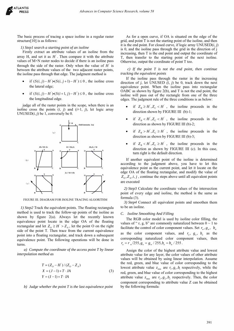
1) Step2 Track the equivalent points. The floating rectangula method is used to track the follow-up points of the isoline as shown by figure 2(a). Always let the recently known equivalence point locate in the edge OA of the floating rectangular and let '

O AZ H Z , let the point O on the right side of the point T. Then trace from the current equivalence point into a floating rectangular, and track down a subsequent equivalence point. The following operations will be done in turns.

a) Compute the coordinate of the access point T by linear interpolation method as

'( ) / ( )

( 1)

( 1)

O O AT Z H Z Z

X J T JA

Y I T IA

b) Judge whether the point T is the last equivalence point

As for a open curve, if OA is situated on the edge of the grid, and point T is not the starting point of the isoline, and then it is the end point. For closed curve, if logic array UNUSED(i, j) is 0, and the isoline pass through the grid in the direction of j increasing, then T is the end point and output the coordinate of T, then transfer to the starting point of the next isoline. Otherwise, output the coordinate of point T too.

c) If the point T is not the end point, then continue tracking the equivalent points

If the isoline pass through the raster in the increasing direction of j, let UNUSED (i, j) be 0, track down the next equivalence point. When the isoline pass into rectangular OABC as shown by figure 2(b), and T is not the end point, the isoline will pass out of the rectangle from one of the three edges. The judgment rule of the three conditions is as below:

if ' ',B CZ H Z H , the isoline proceeds in the direction shown by FIGURE III (b)-1;

if ' ',B CZ H Z H , the isoline proceeds in the direction as shown by FIGURE III (b)-2;

if ' ',B CZ H Z H , the isoline proceeds in the direction as shown by FIGURE III (b)-3;

if ' ',B CZ H Z H , the isoline proceeds in the direction as shown by FIGURE III (c). In this case, turn right is the default direction.

If another equivalent point of the isoline is determined according to the judgment above, you have to let this equivalence point as the current point, and let it locate on the edge OA of the floating rectangular, and modify the value of

, , ,O AZ Z i j , continue the steps above until all equivalent points are executed

2) Step3 Calculate the coordinate values of the intersection point of every edge and isoline, the method is the same as formula (3).

3) Step4 Connect all equivalent points and smoothen them to be an isoline.

C. Isoline Smoothing And Filling

The RGB color model is used by isoline color filling, the values of “ r, g, b” are commonly naturalized between 0 ~ 1 to facilitate the control of color component values. Set , ,w w wr g b

as the color component values, and , ,o o or g b as the corresponding naturalized color component values, then

/255, / 255, / 255o w o w o wr r g g b b .

Assign the color of the highest attribute value and lowest attribute value for any layer, the color values of other attribute values will be obtained by using linear interpolation. Assume the red, green, and blue value of color corresponding to the lowest attribute value minz are 1 1 1, ,r g b respectively, while the red, green, and blue value of color corresponding to the highest attribute value maxz are 2 2 2, ,r g b respectively. Then, the color component corresponding to attribute value Z can be obtained by the following formula:


391

1 2 1 min max min

1 2 1 min max min

1 2 1 min max min

( ) ( ) / ( )

( ) ( ) / ( )

( ) ( ) / ( )

r r r r z z z z

g g g g z z z z

b b b b z z z z

By isoline tracing algorithm and isoline filling algorithm, the color transition of the generated electromagnetic situation maps is smooth.

IV. CALCULATION EXAMPLE AND COMPUTATIONAL

EFFICIENCY ANALYSIS

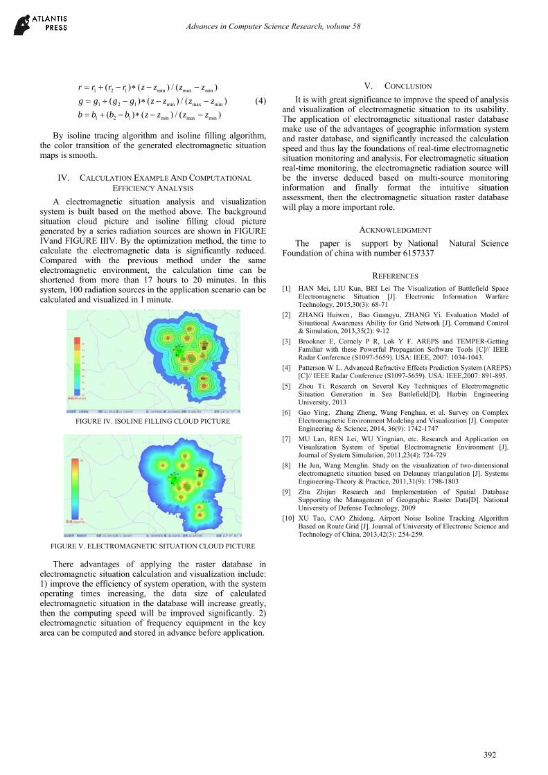
A electromagnetic situation analysis and visualization system is built based on the method above. The background situation cloud picture and isoline filling cloud picture generated by a series radiation sources are shown in FIGURE IVand FIGURE IIIV. By the optimization method, the time to calculate the electromagnetic data is significantly reduced. Compared with the previous method under the same electromagnetic environment, the calculation time can be shortened from more than 17 hours to 20 minutes. In this system, 100 radiation sources in the application scenario can be calculated and visualized in 1 minute.

FIGURE IV. ISOLINE FILLING CLOUD PICTURE

FIGURE V. ELECTROMAGNETIC SITUATION CLOUD PICTURE

There advantages of applying the raster database in electromagnetic situation calculation and visualization include: 1) improve the efficiency of system operation, with the system operating times increasing, the data size of calculated electromagnetic situation in the database will increase greatly, then the computing speed will be improved significantly. 2) electromagnetic situation of frequency equipment in the key area can be computed and stored in advance before application.

V. CONCLUSION

It is with great significance to improve the speed of analysis and visualization of electromagnetic situation to its usability. The application of electromagnetic situational raster database make use of the advantages of geographic information system and raster database, and significantly increased the calculation speed and thus lay the foundations of real-time electromagnetic situation monitoring and analysis. For electromagnetic situation real-time monitoring, the electromagnetic radiation source will be the inverse deduced based on multi-source monitoring information and finally format the intuitive situation assessment, then the electromagnetic situation raster database will play a more important role.

ACKNOWLEDGMENT

The paper is support by National Natural Science Foundation of china with number 6157337

REFERENCES [1] HAN Mei, LIU Kun, BEI Lei The Visualization of Battlefield Space

Electromagnetic Situation [J]. Electronic Information Warfare Technology, 2015,30(3): 68-71

[2] ZHANG Huiwen，Bao Guangyu, ZHANG Yi. Evaluation Model of Situational Awareness Ability for Grid Network [J]. Command Control & Simulation, 2013,35(2): 9-12

[3] Brookner E, Cornely P R, Lok Y F. AREPS and TEMPER-Getting Familiar with these Powerful Propagation Software Tools [C]// IEEE Radar Conference (S1097-5659). USA: IEEE, 2007: 1034-1043.

[4] Patterson W L. Advanced Refractive Effects Prediction System (AREPS) [C]// IEEE Radar Conference (S1097-5659). USA: IEEE,2007: 891-895.

[5] Zhou Ti. Research on Several Key Techniques of Electromagnetic Situation Generation in Sea Battlefield[D]. Harbin Engineering University, 2013

[6] Gao Ying，Zhang Zheng, Wang Fenghua, et al. Survey on Complex Electromagnetic Environment Modeling and Visualization [J]. Computer Engineering ＆ Science, 2014, 36(9): 1742-1747

[7] MU Lan, REN Lei, WU Yingnian, etc. Research and Application on Visualization System of Spatial Electromagnetic Environment [J]. Journal of System Simulation, 2011,23(4): 724-729

[8] He Jun, Wang Menglin. Study on the visualization of two-dimensional electromagnetic situation based on Delaunay triangulation [J]. Systems Engineering-Theory & Practice, 2011,31(9): 1798-1803

[9] Zhu Zhijun Research and Implementation of Spatial Database Supporting the Management of Geographic Raster Data[D]. National University of Defense Technology, 2009

[10] XU Tao, CAO Zhidong. Airport Noise Isoline Tracking Algorithm Based on Route Grid [J]. Journal of University of Electronic Science and Technology of China, 2013,42(3): 254-259.


392

Documents

Analysis and Visualization of Electromagnetic Situation