Analysis and optimization of physical models for HIL ...l2ep.univ-lille1.fr/hil2016/presentations/2.1-HIL-16.pdf · Analysis and optimization of physical models for HIL simulation

Restricted © Siemens AG 2014 All rights reserved. Smarter decisions, better products.

Analysis and optimization of physical

models for HIL simulation

Mathieu Dutré - Application Specialist MBSE

2015-04-15

Restricted © Siemens AG 2014 All rights reserved.

Page 2 Siemens PLM Software

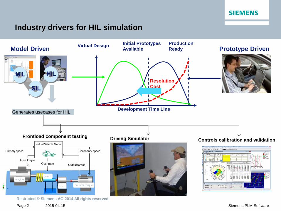
Industry drivers for HIL simulation

Controls calibration and validation Driving Simulator Frontload component testing

Model Driven Prototype Driven Virtual Design

Production

Ready

Initial Prototypes

Available

Development Time Line

Resolution

Cost

Generates usecases for HIL

2015-04-15



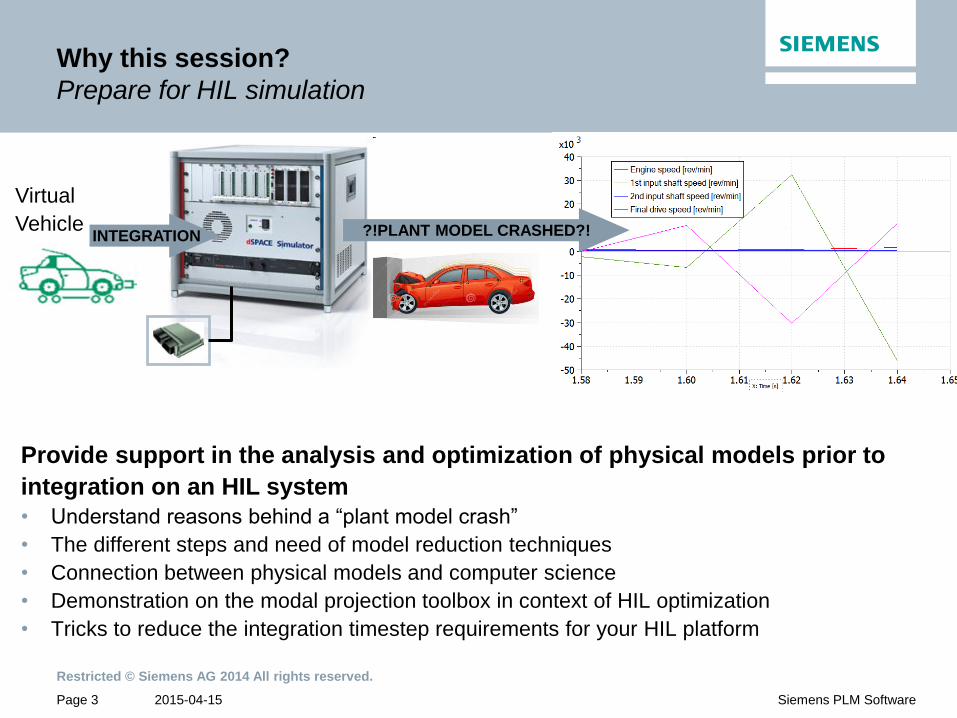
Why this session?

Prepare for HIL simulation

Provide support in the analysis and optimization of physical models prior to

integration on an HIL system

• Understand reasons behind a “plant model crash”

• The different steps and need of model reduction techniques

• Connection between physical models and computer science

• Demonstration on the modal projection toolbox in context of HIL optimization

• Tricks to reduce the integration timestep requirements for your HIL platform

INTEGRATION ?!PLANT MODEL CRASHED?!

Virtual

Vehicle

2015-04-15



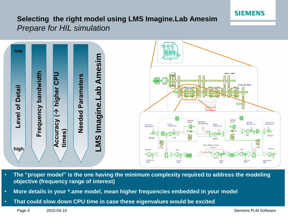
Selecting the right model using LMS Imagine.Lab Amesim


low

high LM

S Im

ag

ine

.La

b A

me

sim

• The “proper model” is the one having the minimum complexity required to address the modeling

objective (frequency range of interest)

• More details in your *.ame model, mean higher frequencies embedded in your model

• That could slow down CPU time in case these eigenvalues would be excited

2015-04-15



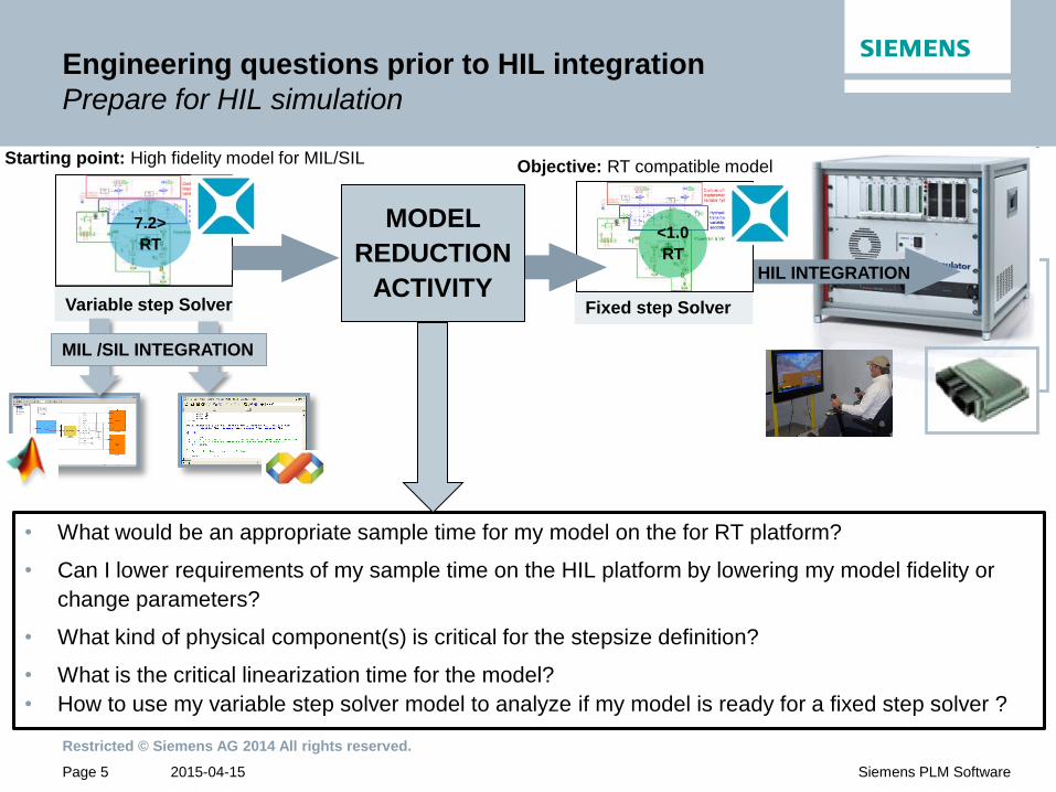
Engineering questions prior to HIL integration


• What would be an appropriate sample time for my model on the for RT platform?

• Can I lower requirements of my sample time on the HIL platform by lowering my model fidelity or

change parameters?

• What kind of physical component(s) is critical for the stepsize definition?

• What is the critical linearization time for the model?

• How to use my variable step solver model to analyze if my model is ready for a fixed step solver ?

HIL INTEGRATION

Fixed step Solver Variable step Solver

7.2>

RT <1.0

RT

MODEL

REDUCTION

ACTIVITY

Starting point: High fidelity model for MIL/SIL Objective: RT compatible model

MIL /SIL INTEGRATION

2015-04-15



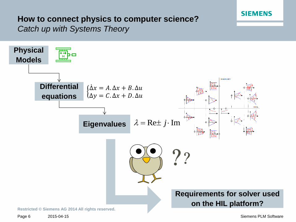
How to connect physics to computer science?

Catch up with Systems Theory

Physical

Models

Differential

equations

Eigenvalues

Requirements for solver used

on the HIL platform?

Δ 𝑥 = 𝐴. Δ𝑥 + 𝐵. Δ𝑢Δ𝑦 = 𝐶. Δ𝑥 + 𝐷. Δ𝑢

ImRe j

2015-04-15



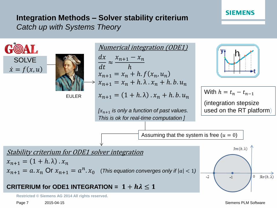
Integration Methods – Solver stability criterium


With ℎ = 𝑡𝑛 − 𝑡𝑛−1

(integration stepsize

used on the RT platform)

Assuming that the system is free (𝑢 = 0)

SOLVE

𝑥 = 𝑓 𝑥, 𝑢

Numerical integration (ODE1)

𝑑𝑥

𝑑𝑡≈𝑥𝑛+1 − 𝑥𝑛

ℎ

𝑥𝑛+1 = 𝑥𝑛 + ℎ. 𝑓 𝑥𝑛, 𝑢𝑛 𝑥𝑛+1 = 𝑥𝑛 + ℎ. λ . 𝑥𝑛 + ℎ. 𝑏. 𝑢𝑛

𝑥𝑛+1 = 1 + ℎ. λ . 𝑥𝑛 + ℎ. 𝑏. 𝑢𝑛

[𝑥𝑛+1 is only a function of past values.

This is ok for real-time computation ]

EULER

Stability criterium for ODE1 solver integration

𝑥𝑛+1 = 1 + ℎ. λ . 𝑥𝑛

𝑥𝑛+1 = 𝑎. 𝑥𝑛 Or 𝑥𝑛+1 = 𝑎𝑛. 𝑥0 (This equation converges only if 𝑎 < 1)

CRITERIUM for ODE1 INTEGRATION = 𝟏 + 𝒉𝝀 ≤ 𝟏

h

2015-04-15



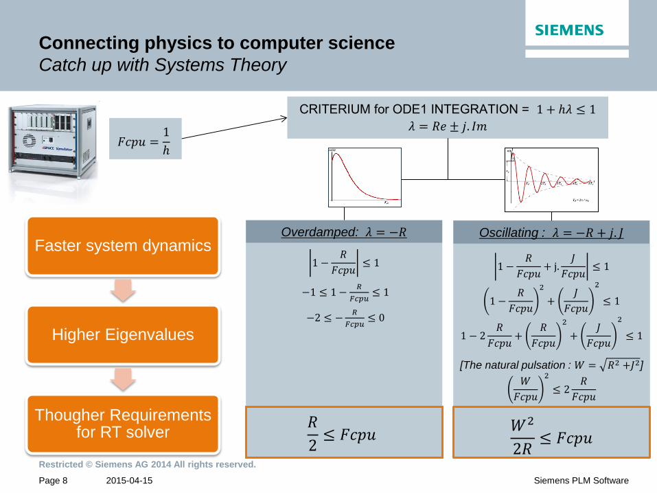
Connecting physics to computer science


1 −𝑅

𝐹𝑐𝑝𝑢+ j.

𝐽

𝐹𝑐𝑝𝑢≤ 1

1 −𝑅

𝐹𝑐𝑝𝑢

2

+𝐽

𝐹𝑐𝑝𝑢

2

≤ 1

1 − 2𝑅

𝐹𝑐𝑝𝑢+

𝑅

𝐹𝑐𝑝𝑢

2

+𝐽

𝐹𝑐𝑝𝑢

2

≤ 1

[The natural pulsation : 𝑊 = 𝑅2 +𝐽2]

𝑊

𝐹𝑐𝑝𝑢

2

≤ 2𝑅

𝐹𝑐𝑝𝑢

𝐹𝑐𝑝𝑢 =1

ℎ

CRITERIUM for ODE1 INTEGRATION = 1 + ℎ𝜆 ≤ 1

𝜆 = 𝑅𝑒 ± 𝑗. 𝐼𝑚

1 −𝑅


−1 ≤ 1 −𝑅


−2 ≤ −𝑅


Faster system dynamics

Higher Eigenvalues

Thougher Requirements for RT solver

Oscillating : 𝜆 = −𝑅 + 𝑗. 𝐽 Overdamped: 𝜆 = −𝑅

𝑅

2≤ 𝐹𝑐𝑝𝑢

𝑊2

2𝑅≤ 𝐹𝑐𝑝𝑢

2015-04-15



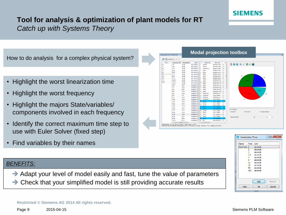
Tool for analysis & optimization of plant models for RT


Adapt your level of model easily and fast, tune the value of parameters

Check that your simplified model is still providing accurate results

Modal projection toolbox

How to do analysis for a complex physical system?

• Highlight the worst linearization time

• Highlight the worst frequency

• Highlight the majors State/variables/

components involved in each frequency

• Identify the correct maximum time step to

use with Euler Solver (fixed step)

• Find variables by their names

BENEFITS:

2015-04-15



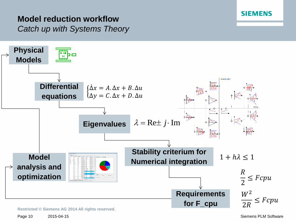
Model reduction workflow


Physical

Models

Differential

equations

Eigenvalues

Requirements

for F_cpu

Model

analysis and

optimization

Stability criterium for

Numerical integration

Δ 𝑥 = 𝐴. Δ𝑥 + 𝐵. Δ𝑢Δ𝑦 = 𝐶. Δ𝑥 + 𝐷. Δ𝑢

𝑅

2≤ 𝐹𝑐𝑝𝑢

𝑊2

2𝑅≤ 𝐹𝑐𝑝𝑢

ImRe j

1 + ℎ𝜆 ≤ 1

2015-04-15



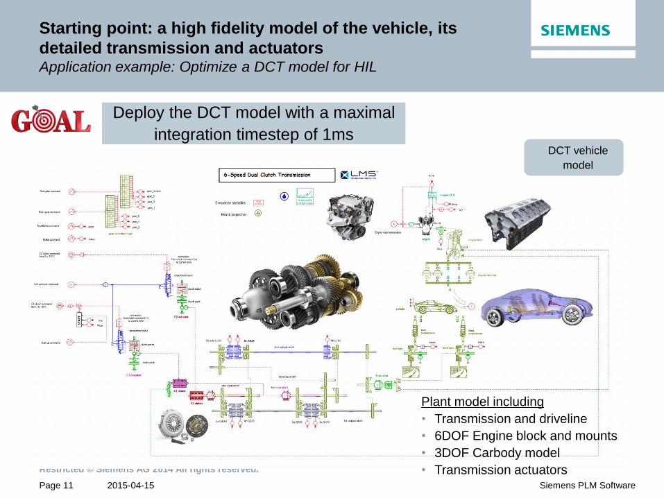
Starting point: a high fidelity model of the vehicle, its

detailed transmission and actuators Application example: Optimize a DCT model for HIL

DCT vehicle

model

Plant model including

• Transmission and driveline

• 6DOF Engine block and mounts

• 3DOF Carbody model

• Transmission actuators

Deploy the DCT model with a maximal

integration timestep of 1ms

2015-04-15



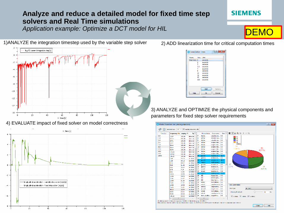
Analyze and reduce a detailed model for fixed time step solvers and Real Time simulations Application example: Optimize a DCT model for HIL

1)ANALYZE the integration timestep used by the variable step solver 2) ADD linearization time for critical computation times

3) ANALYZE and OPTIMIZE the physical components and

parameters for fixed step solver requirements

4) EVALUATE impact of fixed solver on model correctness

DEMO

2015-04-15



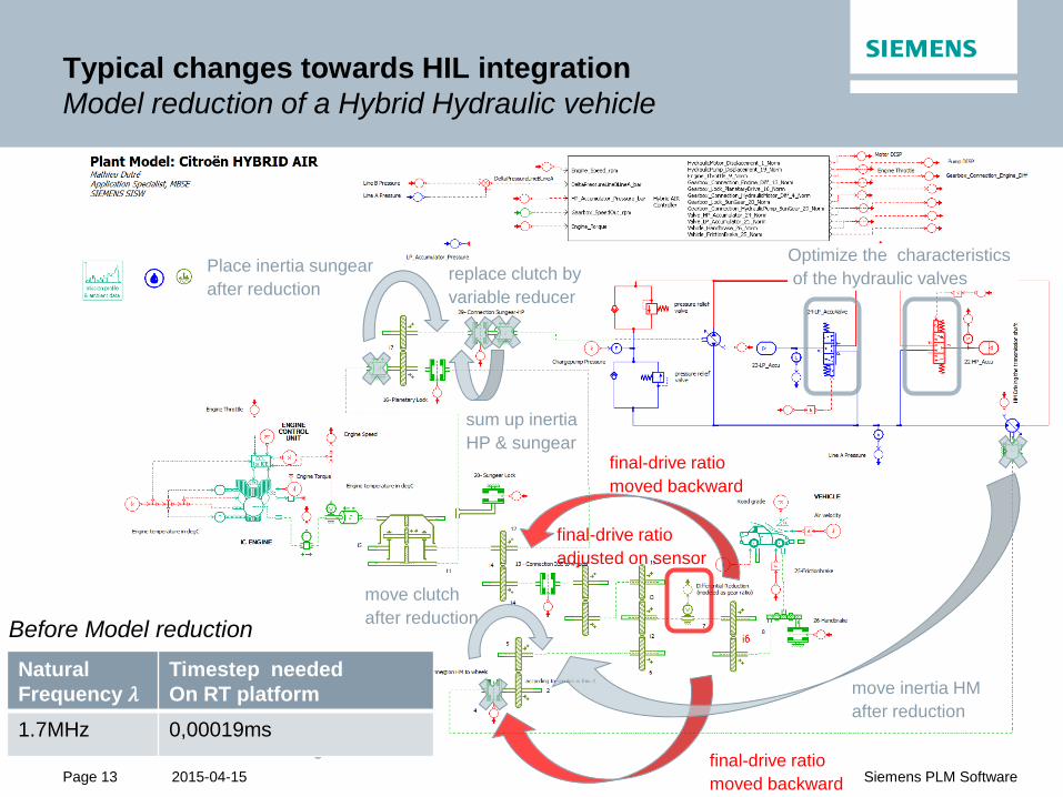
Typical changes towards HIL integration

Model reduction of a Hybrid Hydraulic vehicle

Place inertia sungear

after reduction

sum up inertia

HP & sungear

replace clutch by

variable reducer

move inertia HM

after reduction

move clutch

after reduction

final-drive ratio

moved backward

final-drive ratio

moved backward

final-drive ratio

adjusted on sensor

Optimize the characteristics

of the hydraulic valves

Natural

Frequency 𝜆

Timestep needed

On RT platform

1.7MHz 0,00019ms

Before Model reduction

2015-04-15



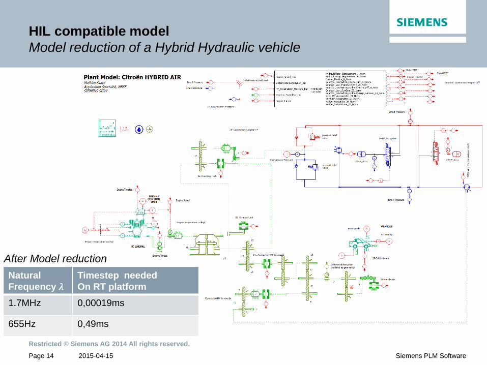
HIL compatible model

Model reduction of a Hybrid Hydraulic vehicle

After Model reduction

Natural

Frequency 𝜆

Timestep needed

On RT platform

1.7MHz 0,00019ms

655Hz 0,49ms

2015-04-15



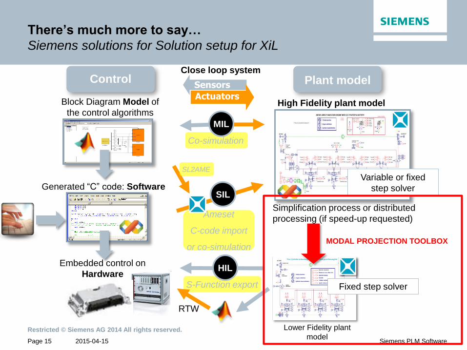
There’s much more to say…

Siemens solutions for Solution setup for XiL

Close loop system

Sensors

Actuators Block Diagram Model of

the control algorithms High Fidelity plant model

Variable or fixed

step solver

Control

Lower Fidelity plant

model

Fixed step solver

Simplification process or distributed

processing (if speed-up requested)

Embedded control on

Hardware

Generated “C” code: Software

Co-simulation

MIL

Plant model

Ameset

C-code import

or co-simulation

SL2AME

SIL

S-Function export

RTW

HIL

MODAL PROJECTION TOOLBOX

2015-04-15



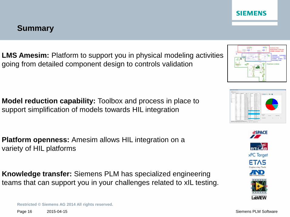
Summary

LMS Amesim: Platform to support you in physical modeling activities

going from detailed component design to controls validation

Model reduction capability: Toolbox and process in place to

support simplification of models towards HIL integration

Platform openness: Amesim allows HIL integration on a

variety of HIL platforms

Knowledge transfer: Siemens PLM has specialized engineering

teams that can support you in your challenges related to xIL testing.

Restricted © Siemens AG 2014 All rights reserved. Smarter decisions, better

products.

Thank you! Questions?

Mathieu DUTRE

Application Specialist, MBSE

[email protected]

+32472409225

mailto:[email protected]

Documents

Analysis and optimization of physical models for HIL ...l2ep.univ-lille1.fr/hil2016/presentations/2.1-HIL-16.pdf · Analysis and optimization of physical models for HIL simulation