Embed Size (px)
Citation preview

Analysis and Numerical Investigation ofDynamic Models for Liquid Chromatography
Dissertation
zur Erlangung des akademischen Grades
doctor rerum naturalium
(Dr. rer. nat.)
von MS Math. Shumaila Javeed
geb. am 29. Januar 1985 in Rawalpindi, Pakistan
genehmigt durch die Fakultat fur Mathematik
der Otto-von-Guericke-Universitat Magdeburg
Gutachter:
Prof. Dr. Gerald Warnecke
Prof. Dr. Thomas Sonar
Eingereicht am: 19.11.2012
Verteidigung am: 25.06.2013


AbstractIn this work models capable to describe non-reactive and reactive liquid chromatography
are investigated numerically and theoretically. These models have a wide range of industrial
applications e.g. to produce pharmaceuticals, food ingredients, and fine chemicals. Two
established models of liquid chromatography, the equilibrium dispersive model and the
lumped kinetic model, are analyzed using Dirichlet and Robin boundary conditions to solve
the column balances. The models consist of systems of convection-diffusion-reaction partial
differential equations with dominating convective terms coupled via differential or algebraic
equations. The Laplace transformation is used to solve them analytically for the special case
of single component linear adsorption. Statistical moments of step responses are calculated
and compared with numerical predictions generated by using the methods studied in this
thesis for both sets of boundary conditions. For nonlinear adsorption isotherms, only
numerical techniques provide solutions. However, the strong nonlinearities of realistic
thermodynamic functions and the stiffness of reaction terms pose major difficulties for the
numerical schemes. For this reason, computational efficiency and accuracy of numerical
methods are of large relevance and a focus of this work. Another goal is to analyze the
influence of temperature gradients on reactive liquid chromatography, which are typically
neglected in theoretical studies. By parametric calculations the influence of temperature
gradients on conversion and separation processes during reactive liquid chromatography are
analyzed systematically. Additionally, the complex coupling of concentration and thermal
fronts is illustrated and key parameters influence the reactor performance are identified.
Two numerical schemes, namely the finite volume scheme of Koren and the discontinuous
Galerkin finite element method, are applied to numerically approximate the models con-
sidered. These schemes give a high order accuracy on coarse grids, resolve sharp fronts,
and avoid numerical diffusion and dispersion. Several case studies to analyze non-reactive
and reactive liquid chromatographic processes are carried out. The results of the suggested
numerical methods are validated qualitatively and quantitatively against some finite vol-
ume schemes from the literature. The results achieved verify that the proposed methods
are robust and well suited for dynamic simulations of chromatographic processes.


ZusammenfassungIn dieser Arbeit geht es um die numerische und theoretische Untersuchung von Modellen,
welche die reaktive und die nichtreaktive Flussig-Chromatographie beschreiben. Diese
Modelle finden in einem großen Rahmen industrielle Anwendungen, z.B. bei der Pro-
duktion von Arzneimitteln, Nahrungsmitteln und Feinchemikalien. Zwei gangige Mod-
elle der Flussig-chromatographie, das “Equilibrium Dispersive Model” und das “Lumped
Kinetic Model”, werden mit Hilfe der von Dirichlet- und Robin-Randbedingungen unter-
sucht. Die Modelle bestehen aus Systemen von partiellen Differentialgleichungen, welche
die Konvektions-Diffusions-Reaktion sprozesse beschreiben, bei denen der konvektive Term
dominiert und die mit Differentialgleichungen oder algebraischen Gleichungen gekoppelt
werden. Um diese modellgleichungen analytisch fur den Spezialfall der linearen Adsorption
von Einzelkomponenten zu losen, wird die Laplace-Transformation benutzt. Dabei werden
die statistischen Momente der Ubergangsfunktion berechnet und mit den numerischen Vo-
raussagen verglichen, die mit Hilfe der hier untersuchten Methoden fur beide Randbedin-
gungen gewonnen wurden. Fur nichtlinearen Adsorptionsisothermen konnen Losungen nur
mit numerischen Methoden gewonnen werden. Die starke Nichtlinearitat von realen ther-
modynamischen Funktionen und die Steifigkeit der Reaktionsterme stellen im Allgemeinen
eine große Schwierigkeit fur numerischen Methoden dar. Aus diesem Grund stehten die
Effizienz bei der Berechnung sowie die Genauigkeit der numerischen Methoden im Fokus
dieser Arbeit. Ein weiteres Ziel ist die Analyse des Einflusses von Temperaturgradienten auf
die reaktive Flussig-chromatographie, welcher bicher in theoretischen Arbeiten nur selten
betrachtet werden. Mit Hilfe von parametrischen Berechnungen wurde der Einfluss von
Temperaturgradienten auf Konversions- und Seperationsprozesse, die wahrend der reak-
tiven Flussigchromatographie stattfinden, systematisch untersucht. Zusatzlich wird die
komplexe Kopplung von Konzentrations- und Warmefronten erklart und es die werden
Parameter identifiziert, die einen wesentlichen Einfluss auf die Reaktorleistung haben.
Zwei numerische Methoden, die Finite Volumenmethode von Koren und die diskontinuier-
liche Galerkin-Finite-Elementemethode, werden hier vorgeschlagen, um die betrachteten

Modellgleichungen numerisch zu approximieren. Diese Methoden erlauben eine hohe Genau-
igkeit auf groben Gittern, losen scharfe Fronten auf und vermeiden numerische Diffu-
sion und Dispersion. Es wurden verschiedene Fallstudien durchgefuhrt, um reaktive und
nichtreaktive chromatographische Prozesse zu analysieren. Die mit den hier vorgeschlage-
nen Methoden erreichten Ergebnisse wurden qualitativ und quantitativ im Vergleich mit
von Resultaten der Finiten-Volumen-Methoden aus der Literatur validiert. Die Ergeb-
nisse zeigen, dass die hier vorgeschlagenen Methoden robust und gut geeignet sind fur die
dynamische Simulation von chromatographischen Prozessen.
Acknowledgments
This thesis originated during my tenure as a Research Scholar at the Max Planck Institute
for Dynamics of Complex Technical Systems in Magdeburg, Germany.
First and foremost, I am grateful to my supervisor Prof. Gerald Warnecke who always
encouraged me and gave me remarkable suggestions and invaluable supervision throughout
my thesis work. His advices, constructive criticism and kind behavior have always been
the driving force towards the successful completion of research projects.
I am highly indebted to Prof. Andreas Seidel-Morgenstern, who gave me a chance to work
at the Max Planck Institute Magdeburg and to utilize its excellent research platform. His
valuable advice, kind attitude, constant encouragement, technical discussions have helped
me immensely to improve my research capabilities and to finish the doctoral studies in an
adequate time.
I am pleased to acknowledge my deepest gratitude to Prof. Shamsul Qamar for his guid-
ance, constructive criticism and valuable suggestions during this thesis project.
This thesis would not have been possible without the funding from the International Max
Planck Research School, Magdeburg and the state of Saxony-Anhalt. I am also grateful to
Dr. Jurgen Koch and Dr. Barbara Witter for the support they provided.
I would like to express my heart-felt sense of gratitude to my grandfather Muhammad
Basharat Kiyani (Late). To obtain a PhD degree was my grandfather’s dream for me from
my early childhood. He was the driving force behind my every endeavor throughout my
life. I can never thank him rightfully for his countless love, giving me confidence and high
aims regarding my studies.
I thank my parents, especially my mother, for instilling in me the qualities of integrity and
willingness to always pursue more knowledge. Her endless support, care, and friendship,
are something immeasurable. Thanks to her for bearing my absence, during my stay in
Germany just for my desire to study abroad.
To you my loving brother Wajahat Kiyani, my source of inspiration, my light in the dark.
Thanks for your support, love and extreme desire to complete this degree.


Contents
1 Introduction 1
1.1 Overview . . . . . . . . . . . . . . . . . . . . . . . . . . . . . . . . . . . . 1
1.2 Early development of chromatography . . . . . . . . . . . . . . . . . . . . 4
1.3 Problems and motivation . . . . . . . . . . . . . . . . . . . . . . . . . . . . 4
1.4 Outline of the thesis . . . . . . . . . . . . . . . . . . . . . . . . . . . . . . 9
2 Theory of Chromatography 12
2.1 Overview . . . . . . . . . . . . . . . . . . . . . . . . . . . . . . . . . . . . 12
2.2 Model parameters . . . . . . . . . . . . . . . . . . . . . . . . . . . . . . . . 13
2.2.1 Column porosities . . . . . . . . . . . . . . . . . . . . . . . . . . . . 13
2.2.2 Efficiency . . . . . . . . . . . . . . . . . . . . . . . . . . . . . . . . 15
2.2.3 Adsorption isotherms . . . . . . . . . . . . . . . . . . . . . . . . . . 16
2.3 Continuous chromatographic models . . . . . . . . . . . . . . . . . . . . . 17
2.3.1 The ideal model . . . . . . . . . . . . . . . . . . . . . . . . . . . . . 18
2.3.2 The equilibrium dispersive model (EDM) . . . . . . . . . . . . . . . 19
2.3.3 The lumped kinetic model (LKM) . . . . . . . . . . . . . . . . . . . 19
2.3.4 The general rate model (GRM) . . . . . . . . . . . . . . . . . . . . 20
3 Numerical Schemes 23
3.1 The FVMs formulation for FBCR models . . . . . . . . . . . . . . . . . . . 23
3.2 The DG method formulation for FBCR models . . . . . . . . . . . . . . . 29
ix

x CONTENTS
4 Analytical Solution and Moment Analysis for Linear Models 36
4.1 The lumped kinetic model (LKM) . . . . . . . . . . . . . . . . . . . . . . . 36
4.2 Analytical solutions of EDM and LKM for linear isotherm . . . . . . . . . 37
4.2.1 Analytical solution of EDM . . . . . . . . . . . . . . . . . . . . . . 37
4.2.2 Analytical solution of LKM . . . . . . . . . . . . . . . . . . . . . . 39
4.3 Reduced EDM and LKM: Moment models . . . . . . . . . . . . . . . . . . 40
4.4 Numerical test problems . . . . . . . . . . . . . . . . . . . . . . . . . . . . 43
4.5 Conclusion . . . . . . . . . . . . . . . . . . . . . . . . . . . . . . . . . . . . 51
5 Numerical Solutions of Linear and Non-Linear Chromatographic Models 55
5.1 Numerical test problems . . . . . . . . . . . . . . . . . . . . . . . . . . . . 56
5.1.1 Non-reactive single-component elution . . . . . . . . . . . . . . . . 57
5.1.2 Non-reactive binary elution . . . . . . . . . . . . . . . . . . . . . . 63
5.1.3 Three-component elution . . . . . . . . . . . . . . . . . . . . . . . 72
5.1.4 Four-component reactive elution . . . . . . . . . . . . . . . . . . . . 79
5.2 Conclusion . . . . . . . . . . . . . . . . . . . . . . . . . . . . . . . . . . . . 85
6 Thermal Effects in Reactive Liquid Chromatography 86
6.1 The non-isothermal chromatographic reactor model . . . . . . . . . . . . . 87
6.2 Formulation of numerical scheme . . . . . . . . . . . . . . . . . . . . . . . 91
6.3 Consistency tests for validation . . . . . . . . . . . . . . . . . . . . . . . . 95
6.3.1 Identity of integrated extents of reaction . . . . . . . . . . . . . . . 95
6.3.2 Integrated energy balance considering the extent of reaction . . . . 96
6.4 Demonstrations of thermal effects . . . . . . . . . . . . . . . . . . . . . . . 97
6.4.1 Trivial limiting cases . . . . . . . . . . . . . . . . . . . . . . . . . . 97
6.4.2 Non-trivial test problems . . . . . . . . . . . . . . . . . . . . . . . . 98
6.5 Conclusion . . . . . . . . . . . . . . . . . . . . . . . . . . . . . . . . . . . . 112
7 Summary and Conclusions 113

CONTENTS xi
A Mathematical Derivations 117
B Nomenclature 124
Bibiliography 126
Curriculum Vitae 138


List of Tables
3.1 Different flux limiters used in (3.20). . . . . . . . . . . . . . . . . . . . . . 28
4.1 Analytically determined moments for EDM and LKM. . . . . . . . . . . . 42
4.2 Parameters for Section 4.4. . . . . . . . . . . . . . . . . . . . . . . . . . . . 45
4.3 Errors and CPU times at 50 grid points. . . . . . . . . . . . . . . . . . . . 45
4.4 Errors and CPU times at 100 grid points. . . . . . . . . . . . . . . . . . . . 46
5.1 Section 5.1.1 (Linear isotherm): L1-errors and CPU times of schemes. . . . 59
5.2 Section 5.1.1 (Linear isotherm): L1-errors and EOC of the DG scheme. . . 59
5.3 Section 5.1.1 (Linear isotherm): L1-errors and EOC of the Koren scheme. . 60
5.4 Section 5.1.1 (Linear isotherm): EOC of schemes for Dapp = 0.002 m2/s. . 60
5.5 Section 5.1.1 (Linear isotherm): EOC of schemes for Dapp = 2× 10⁻⁵ m2/s. 60
5.6 Section 5.1.1 (Nonlinear isotherm): L1-errors and CPU times of schemes. . 62
5.7 Section 5.1.2 (case 2): Inlet and initial conditions for problems. . . . . . . . 69
5.8 Section 5.4: Temperature dependent reaction and adsorption parameters. . 83
6.1 Problem 1: Isothermal case study. . . . . . . . . . . . . . . . . . . . . . . . 100
6.2 Problem 2: Influence of the enthalpy of reaction ∆HA,i = 0, EA = 60 kJ/mol.102
6.3 Problem 3: Influence of enthalpy of adsorption ∆HR = 0, EA = 60 kJ/mol.. 104
6.4 Problem 4a: Influence of both enthalpies of reaction and adsorption. . . . . 107
xiii
List of Figures
1.1 Principle of non-reactive and reactive liquid chromatography. . . . . . . . . 3
2.1 Left: linear isotherm, right: nonlinear isotherm. . . . . . . . . . . . . . . . 17
3.1 Cell centered finite volume grid. . . . . . . . . . . . . . . . . . . . . . . . . 24
3.2 Grids near the boundaries. . . . . . . . . . . . . . . . . . . . . . . . . . . . 28
4.1 Comparison of different numerical schemes for LKM. . . . . . . . . . . . . 46
4.2 Dispersion and mass transfer effects. . . . . . . . . . . . . . . . . . . . . . 47
4.3 Comparison of analytical and numerical solutions for Dirichlet conditions. . 48
4.4 Comparison of analytical and numerical solutions for Danckwerts conditions. 48
4.5 Effect of boundary conditions for different values of Peclet number. . . . . 49
4.6 First moments µ1 of EDM and LKM for different flow rates u. . . . . . . . 52
4.7 Second moments µ′
2 for both models, analytical versus numerical results. . 52
4.8 Third moments µ′
3 for both models, analytical versus numerical results. . . 53
5.1 Section 5.1.1 (linear): Comparison of schemes for single component. . . . . 61
5.2 Section 5.1.1 (nonlinear): Comparison of schemes for single component. . . 62
5.3 Section 5.1.1 (nonlinear): Errors at different number of mesh points. . . . . 63
5.4 Section 5.1.2 (case 1): Two-component elution with linear isotherm. . . . . 64
5.5 Section 5.1.2 (case 2a): Riemann problem leads to the S2 − C1 solution. . . 67
5.6 Section 5.1.2 (case 2a): A comparison of the DG and Koren schemes. . . . 68
5.7 Section 5.1.2 (case 2b): Riemann problem leads to the C2 − S1 solution. . . 68
5.8 Section 5.1.2 (case 2c): Riemann problem leads to the C2 − C1 solution. . . 69
xiv

LIST OF FIGURES xv
5.9 Section 5.1.2 (case 2d): Riemann problem leads to the C2 − C1 solution. . 70
5.10 Section 5.1.2 (case 2e): Riemann problem leads to the S2 − S1 solution. . . 70
5.11 Section 5.1.2 (case 2f): Riemann problem leads to the delta-shocks. . . . . 71
5.12 Section 5.1.2 (case 2f): Delta-shocks for different theoretical plate numbers. 71
5.13 Section 5.1.3: 3-component isothermal reactive elution with linear isotherm. 74
5.14 Section 5.1.3: Representation of the operating line. . . . . . . . . . . . . . 76
5.15 Section 5.1.3: Formation of displacement train with cin1 = cin2 = cind = 1 g/l. 77
5.16 Section 5.1.3: A comparison of the DG and Koren schemes. . . . . . . . . . 78
5.17 Section 5.1.3: Displacement chromatography with cind = 0.5 g/l. . . . . . . . 80
5.18 Section 5.1.3: Displacement chromatography with cind = 0.1 g/l. . . . . . . . 80
5.19 Section 5.1.3: A schematic diagram of counter-current adsorption process. . 81
5.20 Section 5.1.3: Displacement chromatography on counter-current bed. . . . 82
5.21 Section 5.1.4: 4-component linear reactive elution at different temperatures. 84
5.22 Section 5.1.4: 4-component nonlinear elution at temperature T = 318. . . . 84
6.1 Trivial limiting case study with ∆HA,i = 0 for i=A,B,C, kfor(Tref) = 0. . . . 99
6.2 Limiting case: Temperature transients for three inlet values. . . . . . . . . 99
6.3 Problem 1: Isothermal case, ∆HA,i = 0, ∆HR = 0. . . . . . . . . . . . . . . 101
6.4 Problem 2: Influence of the enthalpy of reaction, ∆HA,i = 0, for i=A,B,C. . 103
6.5 Problem 3: Influence of enthalpies of adsorption, ∆HR = 0. . . . . . . . . . 105
6.6 Problem 4a: Influence of both enthalpies of reaction and adsorption. . . . . 107
6.7 Problem 4a: Influence of activation energy on the process. . . . . . . . . . 108
6.8 Problem 4b: Enthalpy of adsorption (componentwise). . . . . . . . . . . . 110
6.9 Problem 5: Influence of dispersion terms. . . . . . . . . . . . . . . . . . . . 111


Chapter 1
Introduction
This chapter presents a general overview regarding chromatographic separation processes
and limitations of existing numerical techniques for chromatographic models capable to
describe front propagation phenomena taking place in chromatographic columns. In ad-
dition, numerical solution techniques, such as finite-difference, finite-element and finite
volume methods are briefly reviewed and basic requirements on the quality of numerical
solutions are discussed. Moreover, a short summary of recent relevant results related to
the topic of this work and an outline of the thesis are presented.
1.1 Overview
The separation and purification of components of a mixture are highly important for several
industries. Examples are related to the production of pharmaceuticals, food, and fine
chemicals. Chromatography is one of the most versatile separation techniques widely used
for analysis and purification of multi-component mixtures that are difficult to separate
by conventional separation processes, such as distillation or extraction. Chromatography
is successfully applied to perform numerous complex separation processes, such as the
separation of enantiomers and the isolation from fermentation broths of proteins. It has
a potential to provide the required purities and offers high yield at reasonable production
rates. Chromatography is in particular effective for difficult separation tasks when high
purity products are demanded. The technology has gained immense industrial popularity
1

2 Chapter 1. Introduction
in the past few decades [30].
Reactive chromatography can be an attractive technique to effectively reduce the number
of units and enhance the performance of processes providing pure reaction products. In
reactive chromatography, chemical reactions and chromatographic separation of the prod-
ucts take place simultaneously in the column. This principle is comparable to reactive
distillation, reactive extraction or reactive absorption [85]. The concept is particularly
advantageous to perform equilibrium limited reversible reactions due to the separation
based shifting of chemical equilibrium allowing to improve conversion, yield and separation
efficiency. The reactive chromatography reduces capital investment, energy and operat-
ing costs, equipment sizes and waste. It improves selectivity, purity, and productivity.
Despite several theoretical investigations of reactive chromatography, accurate databases
and models are still lacking for broader commercialization. There are several reviews
available describing the principle and a few applications of chromatographic reactors, e.g.
[4, 24, 25, 80, 102]. The motivation of most current research works is to provide more
profound insight into all aspects for identifying fields of application and for scaling up the
process to industrial relevant sizes.
Chromatographic separation is based on different adsorptivities of the mixture components
to a specific adsorbent which is fixed in a chromatographic column. The simplest process
is batch chromatography involving a single packed column charged with pulses of feed
solution. The injected mixtures are carried through the column by a continuously flowing
desorbent. The components to be separated now move with different velocities in the
column due to their specific affinities with the solid phase. A low retained component
exits the column earlier than a more retained one and, hence, separation is achieved. The
illustration of the chromatography principle is given in Figure 1.1.
Chromatographic reactors were patented in the early 60’s, see e.g. [18, 26, 55]. A packed
bed chromatographic reactor (FBCR) is defined by Langer [47] as a “chromatographic
column in which a solute or several solutes are intentionally converted, either partially or
totally, to products during their residence in the column. The solute reactant or reactant
mixture is injected into the chromatographic reactor as a pulse. Both conversion to product

1.1. Overview 3
space
Co
ncen
tration
Separated componentsDesorbent
Column filled with stationary phase
DetectorPump
Injection(Reactant)
A+B+CA B+C
Figure 1.1: A schematic illustration of the principle of non-reactive and reactive liquidchromatography.
and separation take place in the course of passage through the column; the device is truly
both a reactor and a chromatograph”.
The basic concept of fixed-bed chromatographic reactors can be easily illustrated by con-
sidering a single chromatographic column in which a reversible reaction of the type A
B+C takes place. In reactive chromatography, rectangular pulses of reactant A are peri-
odically fed into the inert carrier stream instead of injecting mixtures in process used just
for separation. Thus, reactant A is transported through the column packed and reacts to
form the products B and C eventually supported by catalytic effects of the solid phase.
Different affinities of components B and C produce different migration velocities of the
products, which leads to their separation, suppresses the backward reaction and provides
high conversion of reactant A at the column outlet, see Figure 1.1. A very favorable situa-
tion exists for this type of reaction, when A elutes between the products B and C. Complete
conversion of A is possible provided the residence in the column is long enough.

4 Chapter 1. Introduction
1.2 Early development of chromatography
Techniques affiliated to chromatography have long been practiced to purify substances, for
instance to purify dyes from plant extracts. The Russian chemist and botanist Michael
Tswett [96, 97] first used the word chromatography to describe the separation of plant
pigments. In his experiment, he used a vertical glass column packed with adsorptive mate-
rials, as alumina or silica. Afterwards, he injected a solution of plant pigments at the upper
end of the column and washed the column with an organic solvent. As a result, a series of
colored pigment bands appeared in the column, separated by regions free from pigments.
Due to these color bands, he named this method chromatography which means color writ-
ing, deduced from the Greek for color-chroma and for write-graphein. His work was largely
ignored until the work of Kuhn et al. [44] on the separation of plant pigments and the
first book published by Zechmeister and Cholnoky [106] on chromatography. The modern
form of chromatography came up in the 1940s and 1950s. A breakthrough in partition
chromatography is due to the work of Martin [57] and related to the subsequent devel-
opment of different chromatography methods such as, paper chromatography, gas-solid
and gas-liquid chromatography and various techniques of column liquid chromatography.
Further advances constantly improved the performance of chromatography and promoted
application for the separation of many complex mixtures.
1.3 Problems and motivation
Mathematical modeling has gained an immense importance in chemical process engineer-
ing. Various mathematical models, defined as an abstraction of the physical world are
developed, considering different levels of complexity to describe the processes. Due to the
exponential increase of computing power in terms of memory size and speed, numerical
simulation has increasingly become a very prominent approach to solve complex practical
problems in engineering and science. Numerical simulation provides an alternative tool
for scientific investigations instead of carrying out expensive, time-consuming or even dan-
gerous experiments in laboratories. The numerical tools are often more valuable than the

1.3. Problems and motivation 5
conventional experimental methods in terms of providing more profound insights and com-
plete information that cannot be directly measured or observed [30, 81].
Standard chromatographic models contain systems of convection-diffusion partial differen-
tial equations with dominating convective terms, coupled with some algebraic equations.
Analytical solutions can be obtained in the Laplace domain for linear models. If no ana-
lytical inversion could be performed, the numerical inversion can be used to generate the
corresponding time domain solutions. Moment analysis is an effective strategy for deducing
important information about the retention equilibrium and mass transfer kinetics in the
column. Such a moment analysis approach has been found frequently instructive in the
literature [30, 41, 42, 43, 62, 63, 64, 65, 76, 82, 87]. The Laplace transformation can be
used as a basic tool to obtain moments. The numerical inverse Laplace transformation of
the equations provides complete elution profiles. The retention equilibrium-constant and
parameters of the mass transfer kinetics in the column are related more simply just to the
moments of these profiles available from the Laplace domain solution.
For nonlinear chromatographic models, analytical solutions cannot be derived. For that
reason, numerical simulations are needed to predict the dynamic behavior of chromato-
graphic columns. Therefore, computational efficiency and accuracy of a numerical method
are of large relevance. However, accurate numerical solutions are difficult to obtain due to
the strong nonlinearity introduced typically by the underlying thermodynamic algebraic
functions (adsorption isotherms). Steep concentration fronts and shock layers may occur
due to the convection dominated partial differential equations (PDEs) of chromatographic
models and, hence, efficient numerical methods are required to obtain accurate and phys-
ically realistic solutions. Moreover, the simulation of reactive chromatography is also a
challenging task for a numerical scheme because of stiffness of the reactive source terms.
These stiff terms may produce rapid variations in the solution and can render numeri-
cal methods unstable, unless the time step sizes are sufficiently small. Thus, an efficient
and accurate numerical technique is needed to avoid excessive dissipation, incorrect phase
speeds, spurious oscillations, and to capture sharp discontinuities of the elution profiles.
Thus, much effort has been invested already to develop appropriate numerical schemes for

6 Chapter 1. Introduction
producing efficient and accurate solutions [30, 51, 84, 89].
Generally, three well-known classes of discretization methods can be used to simulate pro-
cesses, namely the finite difference methods (FDMs), the finite elements methods (FEMs)
and the finite volume methods (FVMs) [30]. In the method of finite differences, the model
equations are approximated by finite difference formulas and different orders of accuracies
can be achieved. An efficient algorithm named as Godunov-Rouchon [75], employs back-
ward difference for the advective term and forward differences for time evolution to solve
the model equations. This algorithm gives more reliable results for single components with
refined specific meshes than for multi-component systems using averaged meshes. More-
over, implementation of the Godunov-Rouchon algorithm in gradient-elution or in reactive
chromatography is not very convenient. In general, classical FDMs may fail at shock
discontinuities because of non-uniqueness of the solution.
Finite element methods are one of the prominent and highly effective techniques for ob-
taining approximate solutions to a wide variety of complex computational problems. The
term finite element was first coined by Clough in 1960 [8]. The first book on the FEMs
by Zienkiewicz and Chung was published in 1967 [109]. In the early 1960s, FEMs received
widespread glory and have been employed to solve a large variety of transport problems
arising in nearly every scientific and engineering problems e.g. solid mechanics, fluids flow,
heat problems, dynamics and electrostatic problems. These methods, e.g. the orthogonal
collocation finite element method (OCFEM), were already applied in the field of chro-
matography [6, 54]. FEMs are more accurate than the finite difference approach, but they
are computationally expensive, and not necessarily conservative locally. Moreover, such
methods are unable to suppress numerical oscillations in convection dominated problems.
To deal with such problems, stabilization procedures e.g. Galerkin/Least-square (GLS)
and Streamline-Upwind/Petrov-Galerkin (SUPG) can be used to eliminate overshoots and
undershoots produced by the convective term [32, 33].
The finite volume methods are well known in the computational dynamics field [20, 46,
50, 66, 68, 94]. They refer to small volumes surrounding the nodal points in the domain
and are capable of enforcing the integral form of conservation laws on each discretized cell.

1.3. Problems and motivation 7
The FVMs were originally developed for nonlinear hyperbolic equations and are natural
candidates to numerically approximate such chromatographic models. The schemes give
high order accuracy on coarse grids, resolve sharp discontinuities, and avoid numerical dis-
persion which may lead to incorrect solutions [50]. FVMs, which preserve such properties,
were already applied to simulate different chromatographic processes [16, 51, 60, 103]. In
this thesis, we applied the finite volume method of Koren to chromatographic models and
validated the results with some existing finite volume schemes in the literature [34].
Discontinuous Galerkin (DG) methods belong to the class of finite element methods (FEMs)
which have several advantages over finite difference methods (FDMs) and finite volume
methods (FVMs). For instance, they inherit geometrical flexibility of FVMs and FEMs,
retain the conservation properties of FVMs, and possess the high-order properties of FEMs.
Therefore, DG-methods are locally conservative, stable, and high order accurate. These
methods satisfy the total variation boundedness (TVB) property that guarantees the pos-
itivity of the schemes [9, 11, 12, 108]. Positivity is the most common and fundamental
mathematical requirement in physical models. In our case, concentrations are non-negative
by their nature and their approximations should be non-negative as well. However, nu-
merical solutions of scientific models often generate negative and thus meaningless values.
This may happen even when the numerical method is stable and highly accurate. In fact,
the tendency to produce negative values may, paradoxically, increase with the order of
accuracy of the numerical discretization. Loss of positivity may cause a computation to
fail or produce meaningless results, especially conservation of mass can not be achieved. In
contrast to high order FDMs and FVMs, DG-methods require a simple treatment of the
boundary conditions in order to achieve high order accuracy uniformly. Moreover, DG-
methods allow discontinuous approximations and produce block-diagonal mass matrices
that can be easily inverted through algorithms of low computational cost. These methods
incorporate the idea of numerical fluxes and slope limiters in a very natural way to avoid
spurious oscillations (wiggles), which usually occur due to shocks, discontinuities or sharp
changes in the solution.
The Discontinuous Galerkin finite element method was initially introduced by Reed and

8 Chapter 1. Introduction
Hill [71] for solving neutron transport equations. Afterwards, various DG-methods were
developed and formulated by Cockburn and Shu for nonlinear hyperbolic system in a series
of papers, see for example [9, 11, 12, 13]. DG-methods are being applied in the main stream
of computational fluid dynamic models [1, 2, 3, 7, 14, 31]. The DG-methods are versatile,
flexible, and have intrinsic stability making them suitable for convection dominated prob-
lems. The stability is an intrinsic property of the method to keep the solution bounded, i.e.
numerical errors (roundoff due to finite precision of computers) which are generated during
the solution of discretized equations should not be magnified. The numerical solution itself
should remain uniformly bounded. The DG-methods can be efficiently applied to partial
differential equations (PDEs) of all kinds, including equations whose type changes within
the computational domain. They were not applied to chromatographic models up to now.
In this work, the Runge-Kutta discontinuous Galerkin (RKDG) method is proposed to
solve the chromatographic processes [35].
Apart from the above mentioned numerical methods a commercial software, named gPROMS
(generalized Process Modeling System) based on difference or orthogonal collocation finite
element methods, is quite common in the chromatography community. This software is able
to solve several chemical processes, but coarse mesh points produce physically unrealistic
numerical oscillations near steep adsorption fronts and refined meshes increase the compu-
tational time [50, 61, 95]. Moreover as a black box solver, it is difficult to make changes
according to the problems requirement in the software. Therefore, search for an efficient
and accurate numerical method is imperative for the correct prediction of chromatographic
fronts with reliable accuracy and low computational time.
In this thesis, different numerical schemes are implemented and analyzed for reactive
chromatographic models. Another focus is theoretical modeling and simulation of non-
isothermal reactive liquid chromatography. Thermal effects are widely discussed in the
case of gas phase reactions in solid packings [21, 27, 40, 104, 105]. In reactive liquid
chromatography, thermal effects are typically not considered and modeling of the process
assumes that effects of heats of sorption and reaction are negligible. Only very few con-
tributions considering thermal effects can be found in the literature [77, 78, 79, 90]. The

1.4. Outline of the thesis 9
purpose of this work is to quantify how temperature gradients can influence conversion
and separation in reactive liquid chromatography. Additionally, the coupling of concentra-
tion and thermal fronts should be illustrated and key parameters influencing the reactor
performance should be identified.
Non-isothermal reactive chromatography can be described by a convection dominated sys-
tem of nonlinear convection-diffusion-reaction type partial differential equations and al-
gebraic equations describing thermodynamic and kinetic phenomena. The corresponding
systems have to be solved numerically because analytical solutions cannot be obtained in
such situations. The simulation of non-isothermal reactive chromatography is a challeng-
ing task for a numerical scheme due to the nonlinearity of the convection-dominated mass
and energy balance equations and because of stiffness of the reactive source terms. Finite
volume schemes were already applied in the chromatographic field [16, 34, 51, 60, 103], but
were never implemented to the complex non-isothermal reactive chromatographic model
considered in this work. This study is an effort to provide more profound insights into
various aspects of non-isothermal reactive chromatography and to contribute to improve
the performance of the process, so that it can be further developed and scaled up.
1.4 Outline of the thesis
The contents of the thesis are arranged in the following manner:
In Chapter 2, the theoretical basis related to chromatography is presented. Moreover,
different chromatographic models with model parameters and adsorption isotherms are
briefly described.
In Chapter 3, a high resolution finite volume scheme is applied for solving chromatographic
models. The third order accuracy of the finite volume scheme is verified by using Taylor
expansion of the solution. To suppress the numerical oscillations and preserve the mono-
tonicity of the scheme a minmod limiter is used. Moreover, the total variation bounded
Runge-Kutta DG-scheme is implemented for the numerical approximation of chromato-
graphic models. The scheme employs a DG-method in the axial-coordinate that converts

10 Chapter 1. Introduction
the given PDE to a system of ordinary differential equations (ODEs). The resulting ODE-
system is then solved by using explicit and nonlinearly stable high order Runge-Kutta
method.
In Chapter 4, the equilibrium dispersive and a non-equilibrium adsorption lumped kinetic
model are solved analytically for linear isotherm. For this purpose, the Laplace transfor-
mation is utilized as a basic tool to transform the PDEs of the models for linear isotherms
to ODEs. The corresponding analytical solutions of EDM and LKM are obtained along
with Dirichlet and Robin boundary conditions (BCs). If no analytical inversion could be
performed, the numerical inversion is used to generate the time domain solution for differ-
ent types of boundary conditions. To analyze the considered linear models, the moment
method is employed to get expressions for retention times, band broadenings and front
asymmetries. In this thesis, a method for describing chromatographic peaks by means of
statistical moments is used and the central moments up to third order are calculated and
compared with numerically obtained moments.
Chapter 5 presents several test problems of isothermal non-reactive and reactive chro-
matographic processes under linear and nonlinear conditions. For linear models, analytical
solutions are obtained in Chapter 4, while for nonlinear models, only numerical techniques
provide solutions. Test Problems are numerically approximated by using the proposed
numerical schemes. The performance of the suggested methods is validated against avail-
able analytical solutions and some other flux-limiting schemes given in the literature. The
case studies include single-component elution, two-component elution, and displacement
chromatography on non-movable (fixed) and movable (counter-current) beds. Moreover,
practical examples of reactive chromatography are also discussed.
Chapter 6 is focused on modeling and simulation of non-isothermal reactive liquid chro-
matography [36]. The model is formed by a system of convection-diffusion-reaction partial
differential equations. To solve this problem, a flux-limiting semi-discrete high resolu-
tion finite volume scheme of Koren [39] is proposed for the numerical approximation of
non-isothermal reactive chromatographic models. The scheme discretizes the model in
axial-coordinate only, while keeps the time variable continuous. The suggested scheme

1.4. Outline of the thesis 11
is found to be second to third order accurate analytically and numerically in our earlier
work of this dissertation on dispersive chromatographic models [34]. Several challenging
case studies are carried out which elucidate the effect of several sources for non-isothermal
behavior. The numerical results were evaluated critically by performing consistency tests
evaluating both mass and energy balances including considerations of limiting cases, which
can be theoretically predicted.
Finally, Chapter 7 is dedicated to the conclusion, remarks and future prospectives of our
research work.
At the end of the thesis we put an appendix. Appendix A presents the derivation of first
three moments for equilibrium dispersive and lumped kinetic models using Dricihlet and
Robin boundary conditions. Appendix B provides a notation for this work.
Most of the content of this thesis is already published in several research journals.
Chapter 3 and 4 consist of
1. Javeed, S., Qamar, S., Ashraf, W., Warnecke, G., Seidel-Morgenstern, A., 2013. Analy-
sis and numerical investigation of two dynamic models of liquid chromatography. Chemical
Engineering Science 90, 17-31.
Chapter 5 summarizes the manuscripts
2. Javeed, S., Qamar, S., Seidel-Morgenstern, A., Warnecke, G., 2011. Efficient and accu-
rate numerical simulation of nonlinear chromatographic processes. Computer & chemical
Engineering 35, 2294-2305.
3. Javeed, S., Qamar, S., Seidel-Morgenstern, A., Warnecke, G., 2011. A discontinuous
Galerkin method to solve chromatographic models. Journal of Chromatography A 1218,
7137-7146.
The results presented in Chapter 6 appeared already in
4. Javeed, S., Qamar, S., Seidel-Morgenstern, A., Warnecke, G., 2012. Parametric study
of thermal effects in reactive liquid chromatography. Chemical Engineering Journal 191,
426-440.
Note that the material for this thesis has been taken from the above mentioned publications
without putting the corresponding text passages in quotation marks.

Chapter 2
Theory of Chromatography
Mathematical models of chromatographic processes are required to predict the migration
behavior of the components in the columns filled with the stationary phases. This chapter
briefly introduces chromatographic standard models describing the process on different
levels of complexity. Moreover, model parameters and adsorption isotherms are introduced.
2.1 Overview
The chromatographic standard models can be mainly divided into three categories, such
as the discrete plate models, continuous models using differential equations and statistical
variants [28].
The plate models equally divide the column length L into a finite number of well mixed
equilibrium stages or theoretical plates, in which the mobile phase is passing through each of
these stages after equilibrium is accomplished. The important examples of plate models are
the continuous plate model proposed by Martin and Synge [57] and the discontinuous plate
model by Craig [15]. In these models, axial dispersion is described by using the number
of theoretical plates and mass transfer effects are typically ignored. The chromatographic
solution profiles of both models are the same for a sufficiently high number of theoretical
plates.
Another prominent modeling approach is the use of continuous models. This approach is
based on differential mass balances of each solute in slices of the column, that leads to a
12

2.2. Model parameters 13
set of partial differential equations. Afterwards, there is a need to find the mathematical
solution of the set of partial differential equations to describe the chromatographic behavior
in a column. Continuous models are further classified into many categories depending on
different levels of complexity of describing the mass transfer and partition processes. Var-
ious mathematical models are available in the literature for understanding and analyzing
dynamic composition fronts in chromatographic columns. The most important of these
models are the general rate model, the lumped kinetic model, the equilibrium-dispersive
model, and the ideal model of chromatography.
The third approach to modeling is a microscopic statistical method for chromatography.
The corresponding models deal with the probability density function for solute molecules
in time and space. An entire discussion on this topic is beyond the scope of this work. For
more details, the readers are referred to consult [19, 81].
2.2 Model parameters
This section focuses on the parameters entering into the chromatographic model equations
presented in the next section. Firstly, the porosity and the efficiency of a column related
to the apparent dispersion coefficient are explained. Afterwards, the adsorption isotherms
are discussed.
2.2.1 Column porosities
The chromatographic column is packed with porous particles. The volume of a column
vcol can be divided into an interstitial volume of mobile phase vm and a stationary phase
volume vst. The stationary phase volume vst can be further divided into two sub-volumes,
such as the solid volume vs and the intraparticle volume of the pores vpore. Thus, the total
volume of the column becomes
vcol = vm + vs + vpore. (2.1)
14 Chapter 2. Theory of Chromatography
On the basis of these volumes two types of porosities, the interstitial porosity ǫint and the
total porosity ǫ can be formulated as
Interstitial porosity: ǫint =vmvcol
, (2.2)
Total porosity: ǫ =vm + vpore
vcol. (2.3)
The volume of a column is given as
vcol =πd2
4L, (2.4)
where, d is diameter of a column, while L represents the length of a column. The interstitial
porosity ǫint is relevant for large molecules, while for small molecules the total porosity ǫ
can be considered. The total porosity can be estimated from the formula given below
ǫ =t0V
vcol, (2.5)
where V is the actual volumetric flow rate of the mobile phase. The t0 denotes the dead
time of the column and can be calculated from the ratio of first and zeroth moments of an
elution profile of a non retained component after a pulse injection is
t0 =
∫∞
0ctdt
∫∞
0cdt
. (2.6)
In this work, the total porosity, c.f. Eq. (2.5), was taken into account.
The Phase ratio (F): The ratio between the volume fractions of the columns which are
occupied by the stationary vst and the mobile phases vm. Using the total porosity ǫ, it is
defined as
F =1− ǫ
ǫ. (2.7)
Linear velocity (u): The linear (or interstitial) velocity u can be calculated from the
subsequent formula, provided the volumetric flow rate V and the total porosity ǫ are
constant.
u =V
ǫπd2
4
. (2.8)

2.2. Model parameters 15
2.2.2 Efficiency
The efficiency of a column is related to the number of theoretical plates Nt. This number
is related to the height equivalent to a theoretical plate (HETP) as
HETP =L
Nt. (2.9)
The number of theoretical plates or HETP can be measured by the statistical moment
method from measured elution profiles. The n-th moment of the chromatographic band
profile denoted by C(x, t) at the exit of column bed of length x = L is
Mn =
∫ ∞
0
C(x = L, t) tndt. (2.10)
The n-th initial normalized moment is
µn =
∫∞
0C(x = L, t) tndt
∫∞
0C(x = L, t)dt
. (2.11)
The second central moment or the variance can be defined as
σ2 = µ′
2 =
∫∞
0C(x = L, t) (t− µ1)
2dt∫∞
0C(x = L, t)dt
. (2.12)
The number Nt can be obtained by considering the first normalized moment µ1 (c.f. Eq.
(2.11)), and the second central moment µ′
2 or variance (σ2) (c.f. Eq. (2.12)), as
Nt =µ21
σ2. (2.13)
For uniformly packed columns with incompressible fluid flow and for an analytical peak
with near Gaussian shape, Nt can be estimated easily as
Nt = 5.54
(tRw1/2
)2
, (2.14)
where tR is the first initial moment of the component peak or the retention time of the
elution profile. Further, w1/2 is the peak width at half height. A dispersion coefficient Dapp
is related for efficient columns to the number of theoretical plates Nt by
Dapp =Lu
2Nt. (2.15)

16 Chapter 2. Theory of Chromatography
The HETP is a function of linear velocity u and can be correlated by the Van Deemter
equation which can be expressed as (e.g. in [98])
HETP = A+B
u+ Cu. (2.16)
In the above equation, A is the eddy diffusion term, B is the axial diffusion term and C is
the mass transfer resistance term. The first term A is influenced by packing imperfections
and by the particle size distributions. The second term B represents the axial diffusion of
the molecules, which can be usually ignored provided the velocity is high enough. The last
term represents a linear dependence with interstitial velocity, where C takes into account
mass transfer resistances, which are unavoidable at very high velocities.
2.2.3 Adsorption isotherms
Isotherms provide thermodynamic information for designing a chromatographic separation
processes and are important to accurately predict the development of concentration profiles
in the column. The adsorption isotherm is the equilibrium relationship between the solute
molecules in the mobile phase and the molecules adsorbed on the surface of the stationary
phase at a constant temperature. This functional relationship is essential to describe the
interactions between the components in the mixture to be separated. By evaluating the
shape of the isotherm, one can distinguish between linear chromatography and nonlinear
chromatography.
In linear chromatography, the equilibrium isotherm is defined by a linear equation given as
q∗i = aici , i = 1, 2, · · · , Nc , (2.17)
where the ai are Henry’s coefficients and Nc represent the number of components in the
sample.
In nonlinear chromatography, the equilibrium relationship between the liquid phase and
solid phase concentrations is nonlinear. A nonlinear effect occurs in most applications of
preparative chromatography. Many nonlinear adsorption isotherm models are available in
the literature, namely Langmuir, Bilangmuir, Freudlich, and Flower models [30]. Nonlinear

2.3. Continuous chromatographic models 17
0 0.5 1 1.5 20
0.5
1
1.5
2
concentration [g/l]
q* [g
/l]
linear isotherm
0 0.5 1 1.5 20
0.05
0.1
0.15
0.2
0.25
concentration [g/l]q*
[g/l]
nonlinear isotherm
Figure 2.1: Left: linear isotherm, right: nonlinear isotherm.
isotherm can have various complex forms. A special case of convex isotherm is the Langmuir
adsorption isotherm, defined for multiple component mixtures as
q∗i =aici
1 +Nc∑
j=1
bjcj
, i = 1, 2, · · · , Nc , (2.18)
where, the ai represent again the Henry’s coefficients and the bj quantify the nonlinearity of
the single component isotherms. For demonstration, plots of linear and nonlinear isotherms
for a single component with a = 1 and b = 4 are displayed in Figure 2.1. At very low
concentrations, the isotherm behaves linearly due to the vanishing influence of the second
term in the denominator of Eq. (2.18), while in case of higher concentrations, the influence
of this denominator becomes significant causing the nonlinearity.
2.3 Continuous chromatographic models
This part explains four well established models of chromatographic columns, namely the
ideal model, the equilibrium-dispersive model, the lumped kinetic model, and the general
rate model of chromatography. These models can be used for both linear and nonlinear
chromatography. All considered models were derived exploiting several basic assumptions
which are listed as follows

18 Chapter 2. Theory of Chromatography
1. The chromatographic process is isothermal.
2. The bed is homogeneous and the packing material used in the stationary phase is
made of porous spherical particles of uniform size.
3. Radial concentration gradients in the column can be neglected.
4. Axial dispersion occurs, and causes band broadening.
5. The mobile phase is considered to be incompressible. This holds for liquid chro-
matography.
6. There is no interaction between the solvent (mobile) and the solid (stationary) phase.
2.3.1 The ideal model
The ideal model assumes that the column has an infinite efficiency. It means that the
axial dispersion is negligible i.e., Dapp = 0, and the thermodynamic equilibrium is achieved
instantaneously. The one dimensional mass balance equation for incompressible fluid and
the isotherm are given as
∂ci∂t
+F∂q∗i∂t
+ u∂ci∂z
= 0 , i = 1, 2, · · · , Nc , (2.19)
q∗i = f (ci) . (2.20)
In the above equations, Nc represents the number of mixture components in the sample,
ci denotes the i-th liquid phase concentration, q∗i is the i-th solid concentration, c.f. Eq.
(2.18), u is the interstitial velocity, F = (1− ǫ)/ǫ is the phase ratio based on the porosity
ǫ ∈]0, 1[, t is time, and z stands for the axial-coordinate. This model provides a first
estimation of the concentration profiles but cannot predict accurately the elution profiles
for low-efficiency columns. In such situations, the contributions of the mass transfer kinetics
and axial dispersion become eminent.
2.3. Continuous chromatographic models 19
2.3.2 The equilibrium dispersive model (EDM)
The equilibrium dispersive model still assumes that the mass transfer is of infinite rate.
Moreover, all contributions due to non-equilibrium and axial dispersion are aggregated into
the corresponding apparent (lumped) dispersion coefficient Dapp. The mass balance equa-
tion of the multi-component equilibrium dispersive model for a fixed bed chromatography
column is written as
∂ci∂t
+ F∂q∗i∂t
+ u∂ci∂z
= Dapp,i∂2ci∂z2
, i = 1, 2, · · · , Nc . (2.21)
Here, Dapp,i represents the i-th apparent axial dispersion coefficient. The EDM predicts the
chromatographic profiles accurately when the column efficiency is high and small particles
are used as the stationary phase in the column. The mass balance equation of the multi-
component fixed-bed chromatographic reactor (FBCR) model adds a reaction term and is
given as
∂ci∂t
+ F∂q∗i∂t
+ u∂ci∂z
= Dapp,i∂2ci∂z2
+ Fνir , i = 1, 2, · · · , Nc , (2.22)
where, r is the rate of the reaction, and the νi are the corresponding stoichiometric coef-
ficients of the components. Note that, the stoichiometric coefficients νi are negative for
reactants and positive for products.
For convenience, the source term in Eq. (2.22) can be re-written as
∂ci∂t
+ F∂q∗i∂t
+ u∂ci∂z
= Dapp,i∂2ci∂z2
+Qi(t, z, c) , i = 1, 2, · · · , Nc . (2.23)
The source term Qi(t, z, c) will be explicitly defined in the test problems discussed in
Chapter 5.
2.3.3 The lumped kinetic model (LKM)
The lumped kinetic model incorporates with the rate of variation of the local concentration
of solute in the stationary phase and local deviation from equilibrium concentrations. The
model lumps the contribution of internal and external mass transport resistances into a

20 Chapter 2. Theory of Chromatography
mass transfer coefficient k. The one-dimensional mass balance laws of a multi-component
LKM are expressed as
∂ci∂t
+ u∂ci∂z
= Di∂2ci∂z2
−kiǫ(q∗i − qi) , (2.24)
∂qi∂t
=ki
1− ǫ(q∗i − qi) , (2.25)
q∗i = f (ci) , i = 1, 2, · · · , Nc . (2.26)
This simple model accounts for the mass transfer kinetics and is more exact than the
equilibrium dispersive model.
2.3.4 The general rate model (GRM)
The GRM considers several contributions of mass transfer kinetics occurring in chromatog-
raphy. As there are several ways to describe these effects, there are many versions of this
model. Usually, axial dispersion, the mass transfer between mobile and stationary phase
and intraparticle the pore diffusion are included in the equations. Also possible limited
rates of adsorption-desorption are often still ignored. The GRM contains two mass balance
equations for the solute, one for inside the particles, and the other for outside the particles.
The mass balance for a fluid percolating through a bed of spherical particles of radius RP
is given as
ǫ∂ci∂t
+ u∂ci∂z
= ǫDi∂2ci∂z2
− (1− ǫ) kexp,iaP × (ci − cP,i(r = RP )) , (2.27)
where, cP,i is the concentration in the particle pores, kexp is the external mass transfer
coefficient, and aP represents the external surface area of the adsorbent particles. The
mass balance inside the particles can be given by
ǫP∂cP,i∂t
+ (1− ǫP )∂q∗i∂t
= Deff,i1
r2∂
∂r
(
r2∂cP,i∂r
)
, (2.28)
where, ǫP is the internal porosity of the particles and theDeff ,i are the effective pore diffusion
coefficients. In principle the GRM has the potential to achieve an accurate description of
chromatographic profiles. However, the implementation and the computation of the GRM

2.3. Continuous chromatographic models 21
is rather expensive and requires many input parameters. Therefore, simplified versions of
the GRM, namely the LKM and the EDM are usually applied to simulate chromatographic
separation processes. For this reason, in this dissertation, the lumped kinetic and the
equilibrium dispersive models are our main concern.
To solve the related mass balance equations given above, appropriate initial and boundary
conditions have to be specified to close the model formulations.
The Initial conditions:
The initial conditions for the liquid phase concentrations typically assume not preloaded
columns as
ci(0, z) = ciniti = ci,0(z), i = 1, 2, · · · , Nc . (2.29)
The corresponding initial conditions used in LKM for fully regenerated columns are given
as
ci(0, z) = 0, qi(0, z) = 0, i = 1, 2, · · · , Nc . (2.30)
Two types of boundary conditions are applied to solve the above second order PDE models.
Boundary conditions of type I: Dirichlet boundary conditions
The Dirichlet boundary conditions at the column inlet is
ci|z=0 = cini (t, 0) = ci,0, i = 1, 2, · · · , Nc . (2.31a)
One useful and realistic outlet condition is
ci(∞, t) = 0, i = 1, 2, · · · , Nc . (2.31b)
Boundary conditions of type II: Robin type boundary conditions
The following more accurate inlet boundary conditions is typically used for models con-
taining dispersion terms [17, 83]. This Robin type of boundary conditions are known in
chemical engineering as Danckwerts conditions
ci|z=0 = ci,0 +Di
u
∂c
∂z
∣∣∣∣z=0
i = 1, 2, 3, · · · , Nc. (2.32a)
22 Chapter 2. Theory of Chromatography
These inlet conditions are usually applied together with the following outlet conditions
∂ci(L, t)
∂z= 0. (2.32b)
Other boundary conditions can also be used to solve the model equations introduced above.
In this thesis, the lumped kinetic model and the equilibrium dispersive model are used
due to their relative simplicity and their demonstrated strength [37]. The finite volume
method of Koren and the discontinuous Galerkin method, presented in the next chapter,
are proposed to numerically approximate these chromatographic models.

Chapter 3
Numerical Schemes
Several numerical schemes have been used in the literature for the approximation of chro-
matographic models [30, 75]. This chapter presents the derivation of two numerical meth-
ods for solving fixed-bed chromatographic reactive (FBCR) models. In section 1, a high
resolution finite volume scheme introduced by Koren [39] is applied for the numerical ap-
proximation of the reactive chromatographic model. In section 2, a discontinuous Galerkin
method is derived for the numerical simulation of reactive chromatographic model.
3.1 The FVMs formulation for FBCR models
This section contains the derivation of the finite volume method of Koren to solve equilib-
rium dispersive model with reaction. The scheme is second to third order accurate in the
axial-coordinate. The order of the scheme is verified analytically during the derivation of
the scheme. For simplicity, a single component equilibrium dispersive model equation with
reaction term, c.f. Eq. (2.23), is taken into account
∂c
∂t+ F
∂q∗
∂t+ u
∂c
∂z= Dapp
∂2c
∂z2+Q(t, z, c) . (3.1)
In the Eq. (3.1), Q(t, z, c) denotes the reaction or source term which will be explicitly
defined in the test problems. If the source or reaction term set equal to zero, i.e. Q(t, z, c) =
0, then Eq. (3.1) leads to the equilibrium dispersive model (c.f. Eq. (2.21)).
23

24 Chapter 3. Numerical Schemes
Let us define w := w(c) = c+ Fq∗(c) and f(c) = uc, the above equation becomes
∂w
∂t+
∂f(c)
∂z= Dapp
∂2c
∂z2+Q(t, z, c) . (3.2)
Before applying the proposed numerical scheme to Eq. (3.2), it is required to discretize
the computational domain. Let N represents the number of discretization points and
(zj− 12)j∈1,··· ,N+1 are partitions of the given interval [0, L]. For each j = 1, 2, · · · , N , ∆z
is a constant width of each mesh interval, zj denote the cell centers, and zj± 12refer to the
cell boundaries, (c.f. Figure 3.1). We assign,
z1/2 = 0 , zN+1/2 = L , zj+1/2 = j ·∆z , for j = 1, 2, · · ·N . (3.3)
Moreover,
zj = (zj−1/2 + zj+1/2)/2 and ∆z = zj+1/2 − zj−1/2 =L
N + 1. (3.4)
zj−1 zj zj+1
zj− 12
zj+ 12
z
Figure 3.1: Cell centered finite volume grid.
Let Ij :=[zj−1/2, zj+1/2
]for i ≥ 1. The cell averaged initial data w0(z) in each cell is given
as
wj(0) =1
∆z
∫
Ij
w0(z) dz , for j = 1, 2, · · ·N . (3.5)
By integrating Eq. (3.2) over the interval Ij =[zj−1/2, zj+1/2
], we obtain
∫
Ij
∂w
∂tdz = −
(
fj+ 12− fj− 1
2
)
+Dapp
((∂c
∂z
)
j+1/2
−
(∂c
∂z
)
j−1/2
)
+
∫
Ij
Q(t, z, c) dz .
(3.6)

3.1. The FVMs formulation for FBCR models 25
In each Ij , the averaged values of the conservative variable w(t) are given as
wj := wj(t) =1
∆z
∫
Ij
w(t, z) dz . (3.7)
Therefore, by using Eq. (3.7) in Eq. (3.6), the following semi-discrete scheme is obtained
dwj
dt= −
fj+ 12− fj− 1
2
∆z+
Dapp
∆z
((∂c
∂z
)
j+ 12
−
(∂c
∂z
)
j− 12
)
+Qj j = 1, 2, · · ·N . (3.8)
Here, N represents the number of mesh points in the domain of computations and differ-
ential terms in the diffusion part can be approximated as
(∂c
∂z
)
j± 12
= ±
(cj±1 − ci
∆z
)
. (3.9)
The next step is to approximate the convective fluxes, fj± 12, in Eq. (3.8) and different
approximations give different numerical schemes. Let us exploit the following inequalities
u > 0 and f > 0.
First order scheme: In this case, the fluxes are approximated as
fj+ 12= fj = (uc)j , fj− 1
2= fj−1 = (uc)j−1 . (3.10)
This approximation gives a first order accurate scheme in the axial-direction.
High resolution schemes: To achieve higher order accuracy, a piecewise interpolation
polynomial can be used, such as
fj+ 12= fj +
1 + κ
4(fj+1 − fj) +
1− κ
4(fj − fj−1) , κ ∈ [−1, 1] . (3.11)
Similarly, fj− 12can be written as
fj− 12= fj−1 +
1 + κ
4(fj − fj−1) +
1− κ
4(fj−1 − fj−2) , κ ∈ [−1, 1] , (3.12)
where, the parameter κ is selected from the interval [−1, 1]. Here, κ = −1 and κ = 1
give second order central schemes, while other values of κ ∈ (−1, 1) give one sided upwind
schemes. Basically, van Leer [100] is the pioneer of κ interpolation schemes.
Truncation error: The following definition is utilized for evaluating the truncation error.

26 Chapter 3. Numerical Schemes
Definition: The truncation error in the interval Ωj is a residual that remains after sub-
stituting the exact solution wj into Eq. (3.8) as
τj(t) :=dwj
dt+
fj+ 12− fj− 1
2
∆z−
Dapp
∆z
((∂c
∂z
)
j+ 12
−
(∂c
∂z
)
j− 12
)
−Qj . (3.13)
Let τ (t) := [τ1(t), τ2(t), · · · , τN (t)]T . The scheme (3.8) is called consistent of order p∗ if,
for ∆z → 0,
‖τ (t)‖ := O(∆zp∗) (3.14)
uniformly for all t. Here, ‖ · ‖ denotes a vector norm in RN .
Let ct :=∂c∂t, fz :=
∂f∂z
and similarly the higher order derivatives. The Taylor expansions of
Eqs. (3.11) and (3.12) at point zj give after some manipulations,
f(t, zj+ 12) =f(t, zj) +
∆z
2(fz)(t, zj) +
κ∆z2
2 · 2!(fzz)(t, zi)
+∆z3
2 · 3!(fzzz)(t, zj) +
κ∆z4
2 · 4!(fzzzz)(t, zj) +O(∆z5) ,
f(t, zj− 12) =f(t, zi)−
∆z
2(fz)(t, zj) +
κ∆z2
2 · 2!(fzz)(t, zj)
+
(
1−3
2κ
)∆z3
3!(fzzz)(t, zj) +
(
−3 −7
2κ
)∆z4
4!(fzzzz)(t, zj) +O(∆z5) .
By putting the above expressions in Eq. (3.13), we get after using Eq. (3.2)
τj(t) :=dw(t, zj)
dt+f(t, zj+ 1
2)− f(t, zj− 1
2)
∆z−
Dapp
∆z
((∂c
∂z
)
j+ 12
−
(∂c
∂z
)
j− 12
)
−Qj
=wt(t, zj) + fz(t, zj)−Dappczz(t, zj)−Qj︸ ︷︷ ︸
=0
+
(3
2κ−
1
2
)∆z2
3!fzzz(t, zi)
+Dapp∆z2
12czzzz(t, zj) +O(∆z3) (3.15)
=
(3
2κ−
1
2
)∆z2
3!fzzz(t, zj)−Dapp
∆z2
12czzzz(t, zj) +O(∆z3) .
For κ = 13
(
1 +Dappczzzz(t,zi)fzzz(t,zi)
)
, one gets a third order accurate scheme, i.e. ‖τ (t)‖ =
O(∆z3). The disadvantage of this κ value is its comparative computational difficulty in
calculating the termczzzz(t,zj)
fzzz(t,zj), especially in the case of difficult flux functions. One can

3.1. The FVMs formulation for FBCR models 27
avoid this problem by considering a higher influence of the advection term as compared
to the dispersion term and can choose κ = 13. This selection of κ is also suitable for the
approximation of current advection dominated dispersive model. However, this assumption
will affect the accuracy of the scheme when the model is diffusion dominated.
Koren scheme: Here, κ = 13is chosen which is third order accurate when there is no
flux-limiting as shown above. For this choice of κ, Eq. (3.11) becomes
fj+ 12= fj +
1
2
(1
3+
2
3
fj+1 − fjfj − fj−1
)
(fj − fj−1) . (3.16)
However, such approximations of flux terms may give negative solutions due to oscillations
in regions of strong variations. To deal with such problems, Koren [39] has used the
following Sweby-type flux-limiter [88],
fj+ 12= fj +
1
2φ(
rj+ 12
)
(fj − fj−1) , (3.17)
where, rj+ 12is the ratio of consecutive flux gradients
rj+ 12=
fj+1 − fj + η
fj − fj−1 + η. (3.18)
Here, η ≈ 10−10 is used to avoid division by zero and the limiting function φ is given as
φ(rj+ 12) = max
(
0,min
(
2rj+ 12,min
(1
3+
2
3rj+ 1
2, 2
)))
. (3.19)
Due to flux-limiting, the above scheme is second to third order accurate [39]. The scheme
gives third order accuracy for a convection dominated equilibrium dispersive model and
gives second order accuracy for a model with very small dispersion coefficient, i.e. when the
model tends to equilibrium case. The same behavior of the scheme is numerically verified
in a test problem.
Other flux-limiting schemes: Several other flux-limiting schemes are available in the
literature. These schemes are different because they involve different flux-limiting functions
[74, 100]. In these schemes, κ = −1 is used in Eqs. (3.11) and (3.12) to obtain fluxes at
the cell boundaries. For example, a limited flux at the right boundary of cell Ij is given as
fj+ 12= fj +
1
2ϕ(
θj+ 12
)
(fj+1 − fj) . (3.20)

28 Chapter 3. Numerical Schemes
Table 3.1: Different flux limiters used in (3.20).Flux limiter Formula
van Leer ([100]) ϕ(r) = |r|+r1+|r|
Superbee ([74]) ϕ(r) = max (0,min(2r, 1),min(r, 2))Minmod ([74]) ϕ(r) = max (0,min(1, r))MC ([100]) ϕ(r) = max
(0,min
(2r, 1
2(1 + r), 2
))
In similar manner, the left cell-boundary flux can be approximated. Here, θj+ 12is the ratio
of consecutive flux gradients
θj+ 12=
fj − fj−1 + η
fj+1 − fj + η. (3.21)
A few well known flux limiters are selected in this study which are listed in Table 3.1. The
efficiency and accuracy of the Koren scheme will be analyzed against these schemes for
selected test problems.
Scheme strategy at the boundaries: The approximations (3.17) and (3.20) are not ap-
plicable to the boundary intervals. Let us consider the left boundary with inflow boundary
condition. The position of the interval face z 12and inflow boundary are identical. However,
z0 is not known, therefore Eqs. (3.17) and (3.20) are not applicable at z 32. To overcome
this problem, the first order approximation (3.10) can be practiced at the cell interfaces z 32
and zN+ 12. Let f in indicates the injected flux, then
f 12= f in , f 3
2= f1, fN+ 1
2= fN . (3.22)
z1 z2 zN−1 zN
z 12
z 32
zN− 12
zN+ 12
z z
a. Inflow. b. Outflow.
Figure 3.2: Grids near the boundaries.
The fluxes at other cell interfaces can be computed by using Eqs. (3.17) or (3.20). However,
the use of a first order scheme in the boundary intervals would not effect the global accuracy
of the method.

3.2. The DG method formulation for FBCR models 29
At each time step, the liquid concentration c is needed for updating the values of isotherm
q∗(c) and flux f(c) = uc. However, Eq. (3.8) gives the updated values of wj(t) = cj(t) +
Fq∗j (c) in each mesh interval Ωj . Therefore, the chain rule can be used in Eq. (3.8) which
gives for j = 1, 2, · · · , N
dcjdt
= −
(
1 + F
(dq∗
dc
)
j
)−1 [fj+ 1
2− fj− 1
2
∆z−
Dapp
∆z
((∂c
∂z
)
j+ 12
−
(∂c
∂z
)
j− 12
)
−Qj
]
.
(3.23)
The resulting system of ODEs can be solved by using any standard ODE-solver. In this
dissertation, the Runge-Kutta 45 method was used to solve the ODE-system, c.f. Eq.
(3.23).
3.2 The DG method formulation for FBCR models
In this section, the TVB Runge-Kutta DG-scheme of Cockburn [9] and Qiu et al. [70] is
implemented for solving the FBCR model given in Eq. (3.1). Firstly, we suitably rewrite
the original system as a degenerate (transformed) first-order system to obtain the weak
formation for deriving the numerical scheme. Then, the TVB Runge-Kutta DG-scheme is
applied in axial-coordinate that converts the given PDE to an ODE-system. The resulting
ODE-system is approximated by using the TVB Runge-Kutta method. For convenience,
one-component FBCR model is considered and is given as
∂c
∂t+ F
∂q∗
∂t+ u
∂c
∂z= Dapp
∂2c
∂z2+Q(t, z, c) . (3.24)
Let us re-write the above equation as
∂
∂t(c+ Fq∗(c)) +
∂
∂z
(
uc−Dapp∂c
∂z
)
= Q(t, z, c) (3.25)
and define
w(c) := c+ Fq∗(c) , g(c) :=√
Dapp∂c
∂z, f(c, g) := uc−
√
Dappg(c) . (3.26)

30 Chapter 3. Numerical Schemes
Then, Eq. (3.25) changes to the following system of PDEs
∂w
∂t= −
∂f
∂z+Q(t, z, c) , (3.27)
g =√
Dapp∂c
∂z. (3.28)
The axial-length variable z is discretized as follows. For j = 1, 2, 3, ....N , let zj+ 12be the
cell partitions, Ij =]zj− 12, zj+ 1
2[ be the domain of cell j, ∆zj = zj+ 1
2− zj− 1
2be the width
of cell j, and I = UIj be the partition of the whole domain. We seek an approximate
solution wh(t, z) to w(t, z) such that for each time t ∈ [0, T ], wh(t, z) belongs to the finite
dimensional space
Vh =v ∈ L1(I) : v|Ij ∈ P p(Ij), j = 1, 2, 3, ....N
, (3.29)
where P p(Ij) denotes the set of polynomials of degree up to p defined on the cell Ij . Note
that in Vh, the functions are allowed to have jumps at the cell interface zj+ 12. In order
to determine the approximate solution wh(t, z), a weak formulation is needed. To obtain
weak formulation, Eqs. (3.27) and (3.28) are multiplied by an arbitrary smooth function
v(z) followed by integration by parts over the interval Ij , we get
∫
Ij
∂w(t, z)
∂tv(z)dz =−
(
f(cj+ 12, gj+ 1
2)v(zj+ 1
2)− f(cj− 1
2, gj− 1
2)v(zj− 1
2))
+
∫
Ij
(
f(c, g)∂v(z)
∂z+Q(t, z, c)v(z)
)
dz, (3.30)
∫
Ij
g(c)v(z)dz =√
Dapp
(
cj+ 12v(zj+ 1
2)− cj− 1
2v(zj− 1
2))
−√
Dapp
∫
Ij
c(z)∂v(z)
∂zdz.
(3.31)
One way to implement (3.29) is to choose Legendre polynomials, Pl(z), of order l as local
basis functions. In this case, the L2-orthogonality property of Legendre polynomials can
be exploited, namely
1∫
−1
Pl(s)Pl′(s) =
(2
2l + 1
)
δll′ . (3.32)

3.2. The DG method formulation for FBCR models 31
For each z ∈ Ij , the solution wh and gh can be expressed as
wh(t, z) =
p∑
l=0
w(l)j ϕl(z) , gh(ch(t, z)) =
p∑
l=0
g(l)j ϕl(z), (3.33)
where
ϕl(z) = Pl (2(z − zj)/∆zj)) , l = 0, 1, ..., p. (3.34)
If p = 0 the approximate solution wh uses the piecewise constant basis functions, if p = 1
the linear basis functions are used, and so on. In this thesis the linear basis functions were
taken into account, therefore l = 0, 1.
By using Eqs. (3.32)-(3.34), it is easy to verify that
w(l)j (t) =
2l + 1
∆zj
∫
Ij
wh(t, z)ϕl(z)dz , g(l)j (t) =
2l + 1
∆zj
∫
Ij
gh(ch)ϕl(z)dz . (3.35)
Then, the smooth function v(z) can be replaced by the test function ϕl ∈ Vh and the
exact solutions w and g by the approximate solutions wh and gh. Moreover, the function
f(cj+ 12, gj+ 1
2) = f(c(t, zj+ 1
2), g(cj+ 1
2)) is not defined at the cell interface zj+ 1
2. Therefore,
it has to be replaced by a numerical flux that depends on two values of ch(t, z), at the
discontinuity, i.e.,
f(cj+ 12, gj+ 1
2) ≈ hj+ 1
2= h(c−
j+ 12
, c+j− 1
2
) . (3.36)
As g := g(c), it can be dropped from the arguments of h for simplicity. Here,
c−j+ 1
2
:= ch(t, z−j+ 1
2
) =
p∑
l=0
c(l)j ϕl(zj+ 1
2) , c+
j− 12
:= ch(t, z+j− 1
2
) =
p∑
l=0
c(l)j ϕl(zj− 1
2) . (3.37)
Using the above definitions, the weak formulations (3.30) and (3.31) simplify to
dw(l)j (t)
dt=−
2l + 1
∆zj
(
hj+ 12ϕl(zj+ 1
2)− hj− 1
2ϕl(zj− 1
2))
+2l + 1
∆zj
∫
Ij
(
f(ch, gh)dϕl(z)
dz+Q(t, z, c)ϕl(z)
)
dz , (3.38)
g(l)j (t) =
2l + 1
∆zj
√
Dapp
cj+ 1
2ϕl(zj+ 1
2)− cj− 1
2ϕl(zj− 1
2)−
∫
Ij
ch(t, z)dϕl(z)
dzdz
. (3.39)

32 Chapter 3. Numerical Schemes
At each time step, the liquid concentration c is needed for updating the values of the
isotherm q∗(c) and flux f(c, g(c)). However, Eq. (3.38) gives the updated values of wj =
cj(t) +Fq∗j (c) in each mesh interval Ij. Therefore, the chain rule can be used in Eq. (3.38)
and the system of ordinary differential equations in terms of cj can be obtained. Thus, the
scheme in Eqs. (3.38) and (3.39) takes the following form
dc(l)j (t)
dt= −
(
1 + F
(dq∗
dc
)(l)
j
)−12l + 1
∆zj
[
hj+ 12ϕl(zj+ 1
2)− hj− 1
2ϕl(zj− 1
2)]
+
(
1 + F
(dq∗
dc
)(l)
j
)−12l + 1
∆zj
∫
Ij
(
f(ch, gh)dϕl(z)
dz+Q(t, z, c)ϕl(z)
)
dz ,
(3.40)
g(l)j (t) =
2l + 1
∆zj
√
Dapp
cj+ 1
2ϕl(zj+ 1
2)− cj− 1
2ϕl(zj− 1
2)−
∫
Ij
ch(t, z)dϕl(z)
dzdz
. (3.41)
The initial data for the above system are given as, c.f. Eq. (3.35),
c(l)j (0) =
2l + 1
∆zj
∫
Ij
c(0, z)ϕl(z)dz , g(l)j (0) = g(c
(l)j (0)) . (3.42)
It remains to choose the appropriate numerical flux function h. The above equation defines
a monotone scheme if the numerical flux function h(a, b) is consistent, h(c, c) = f(c, g(c)),
and satisfies the Lipschitz continuity condition, i.e. h(a, b) is a non-decreasing function of
its first argument and non-increasing function of its second argument. In other words, a
scheme is called monotone if it preserves the monotonicity of the numerical one-dimensional
solution when passing from one time step to another. The following numerical fluxes are
available in the literature, that satisfy the above mentioned properties [46, 50, 107].
(i) The Godunov flux:
hG(a, b) =
mina≤n≤b f(n, g(n)) if a ≤ b,maxa≥n≥b f(n, g(n)) if a > b.
(3.43)
(ii) The Lax-Friedrichs flux:
hLF (a, b) =1
2[f(a, g(a)) + f(b, g(b))− C(b− a)], C = max
inf n0(x)≤s≤supn0(x)|f ′(s, g(s))| .(3.44)

3.2. The DG method formulation for FBCR models 33
(iii) The Local Lax-Friedrichs flux:
hLLF (a, b) =1
2[f(a, g(a)) + f(b, g(b))− C(b− a)], (3.45)
C = maxmin (a,b)≤s≤max (a,b)
|f ′(s, g(s))| . (3.46)
(iv) The Roe flux with ‘entropy fix’:
hR(a, b) =
f(a, g(a)), if f ′(n, g(n)) ≥ 0 for n ∈ [min(a, b),max(a, b)] ,f(b, g(b)), if f ′(n, g(n)) ≤ 0 for n ∈ [min(a, b),max(a, b)] ,
hLLF (a, b) otherwise .(3.47)
In this thesis, we used the Local Lax-Friedrich flux for the investigated models. The Gauss-
Lobatto quadrature rule of order 10 was used to approximate the integral terms appearing
on the right-hand-side of (3.40) and (3.41).
In order to achieve the total variation stability, some limiting procedure has to be intro-
duced. For that purpose, it is needed to modify c±j+ 1
2
in (3.36) by some local projection.
For more details, readers are referred to see e.g. [9]. To this end, we write (3.37) as
c−j+ 1
2
= c(0)j + cj , c+
j− 12
= c(0)j − cj , (3.48)
where
cj =
p∑
l=1
c(l)j ϕl(zj+ 1
2) cj = −
p∑
l=1
c(l)j ϕl(zj− 1
2) . (3.49)
In this study, we consider the linear basis functions, therefore l=0,1. In above equation,
when p = 0, cj = cj = 0 and when p = 1, cj = cj = 6c(1)j etc.
Next, cj and cj can be modified as
c(mod)j = mm
(
cj ,∆+c(0)j ,∆−c
(0)j
)
, c(mod)j = mm
(
cj ,∆+c(0)j ,∆−c
(0)j
)
, (3.50)
where, ∆± := ±(cj±1 − cj) and mm is the usual minmod function defined as
mm(a1, a2, a3) =
s · min1≤i≤3
|ai| if sign(a1) = sign(a2) = sign(a3) = s ,
0 otherwise .(3.51)
Then, Eq. (3.48) modifies to
c−(mod)
j+ 12
= c(0)j + c
(mod)j , c
+(mod)
j− 12
= c(0)j − c
(mod)j (3.52)

34 Chapter 3. Numerical Schemes
and replace (3.36) by
hj+ 12= h(c
−(mod)
j+ 12
, c+(mod)
j− 12
) . (3.53)
This local projection limiter does not affect the accuracy in the smooth regions and conver-
gence can be achieved without oscillations near shocks, see e.g. [9]. Finally, a Runge-Kutta
method that maintains the TVB property of the scheme is needed to solve the resulting
ODE-system. Let us rewrite Eqs. (3.40) and (3.41) in a concise form as
dchdt
= Lh(ch, t) . (3.54)
Then, the r-order TVB Runge-Kutta method can be used to approximate Eq. (3.54)
(ch)p =
p−1∑
l=0
[αpl(ch)
(l) + βpl∆tLh((ch)(l), ts + dl∆t)
], p = 1, 2, · · · , r , (3.55)
where based on Eq. (3.42)
(ch)(0) = (ch)
s , (ch)(r) = (ch)
s+1 . (3.56)
where, s is the s-th time step. For second order TVB Runge-Kutta method the coefficient
are given as (e.g. [9])
α10 = β10 = 1 , α20 = α21 = β21 =1
2, β20 = 0; d0 = 0 , d1 = 1 . (3.57)
While, for the third order TVB Runge-Kutta method the coefficient are given as
α10 = β10 = 1 , α20 =3
4, β20 = 0 , α21 = β21 =
1
4, α30 =
1
3
β30 = α31 = β31 = 0 , α32 = β32 =2
3; d0 = 0 , d1 = 1 , d2 =
1
2. (3.58)
The CFL condition is given as, [9],
∆t ≤
(1
2p+ 1
)
min
(
1 + F
(dq
dc
)(0)
j
)
min
(∆zju
,∆z2j2Dapp
)
, (3.59)
where, p = 1, 2 for second and third order schemes, respectively.

3.2. The DG method formulation for FBCR models 35
Boundary conditions: Let us put the boundary at z− 12= 0. The left boundary condition
given by Eqs. (2.32a) and (2.32b) can be implemented as
c−− 1
2
(t) = c(0)0 +
D
u
c(0)1 − c
(0)0
∆z, (3.60)
c(mod)0 = mm
(
c0,∆+c(0)0 , 2
(
c(0)0 − cin
))
, c(mod)0 = mm
(
c0,∆+c(0)0
)
. (3.61)
Outflow boundary condition is used on the right end of the column, c(l)N+1 = c
(l)N .
In the following chapters, the above models and corresponding numerical schemes will be
used for the simulation of selected chromatographic processes and operation regimes. Re-
turning to the main chromatographic models considered in this work, namely the EDM
and the LKM, can be further classified into two sub-models, i.e., the isotherm function
q∗i = f (ci), depending on the thermodynamic properties. The first simpler case is related
to linear isotherm, Eq. (2.17). In such situations, there exist the possibility to solve the
equation of the EDM and LKM analytically. This will be demonstrated in Chapter 4.
In this chapter, also reduced models based on the statistical moments will be introduced
and provided analytically. The analytical solution give the opportunity for critical valida-
tion of the numerical predictions using the schemes discussed in the current chapter. The
second, more difficult sub-model corresponds to nonlinear isotherm Eq. (2.18). In case
of nonlinear isotherm, no analytical solution can be acquired. Therefore, a validation of
numerical schemes can be done only by comparing with predictions of the schemes. In
Chapter 5, schemes are applied to numerically approximate multi-component nonlinear
chromatographic model equations. The numerical schemes once validated for single com-
ponent linear adsorption in Chapter 4, are seen as powerful tools to simulate a wide range
of processes, c.f. Chapter 5.

Chapter 4
Analytical Solution and MomentAnalysis for Linear Models
This chapter is concerned with the analytical solution of two established models for sim-
ulating liquid chromatographic processes namely, the equilibrium dispersive and lumped
kinetic models. The models are analyzed using Dirichlet and Robin boundary conditions
for linear isotherms. The Laplace transformation is applied to solve these models analyti-
cally for single component adsorption under linear conditions. Statistical moments of step
responses are calculated and compared with the numerical predictions for both types of
boundary conditions.
4.1 The lumped kinetic model (LKM)
The mass balance law of a single component LKM is expressed as
∂c
∂t+ u
∂c
∂z= D
∂2c
∂z2−
k
ǫ(q∗ − q) , (4.1)
∂q
∂t=
k
1− ǫ(q∗ − q) . (4.2)
The three characteristic times in the model Eqs. (4.1)-(4.2) are defined as
τC =L
u, τD =
D
u2, τMT =
1
k. (4.3)
The ratios of these characteristic times provide dimensionless quantities as
τ1 =τCτD
=Lu
D, τ2 =
τCτMT
=Lk
u. (4.4a)
36

4.2. Analytical solutions of EDM and LKM for linear isotherm 37
Here, τ1 typically is frequently called the Peclet number Pe
Pe = τ1 =Lu
D, (4.4b)
where L denotes the length of the column.
For diluted systems or small concentrations, linear isotherms is used and is defined as
q∗ = ac . (4.5)
The equilibrium dispersive model (EDM)-a limiting case of LKM
The basic assumption of EDM is that the kinetics of mass transfer in the chromatographic
column and the kinetics of adsorption-desorption are faster. In Eqs. (4.1) and (4.2), k is
the mass transport coefficient. As the value of k becomes larger, i.e. k → ∞, the model
Eqs. (4.1)-(4.2) change to the equilibrium dispersive model(∂q∂t
= ∂q∗
∂t
)as given below
∂c
∂t+ F
∂q∗
∂t+ u
∂c
∂z= Dapp
∂2c
∂z2. (4.6)
Here, F is the phase ratio related to porosity, i.e. F = 1−ǫǫ, Dapp is the apparent dispersion
coefficient related to the Peclet number by Pe = Lu/Dapp.
4.2 Analytical solutions of EDM and LKM for linear
isotherm
In this section, single component (Nc = 1) linear chromatographic models are considered.
Analytical solutions are derived in a Laplace domain for linear isotherms (Eq. (4.5)) with
Dirichlet (Eq. (2.31a)) and Danckwerts (Eq. (2.32a)) inlet boundary conditions. To simplify
the notations, we consider c(x, t) = c1(x, t).
4.2.1 Analytical solution of EDM
The Laplace transformation is defined as
C(x, s) =
∞∫
0
e−stc(x, t)dt, s > 0. (4.7)

38 Chapter 4. Analytical Solution and Moment Analysis for Linear Models
After normalizing Eq. (4.6) by defining
x = z/L Pe = Lu/Dapp (4.8)
and by applying the Laplace transformation Eq. (4.7) to Eq. (4.6) with Nc = 1 and cinit(t =
0, z) = 0, we obtaind2C
dx2− Pe
dC
dx− sPe
L
u(1 + aF )C = 0 . (4.9)
The solution of this equation is given as
C(x, s) = A exp(λ1x) +B exp(λ2x), (4.10)
λ1,2 =Pe
2∓
1
2
√
Pe2 + 4PeL
u(1 + aF )s . (4.11)
After applying the Dirichlet boundary conditions in Eqs. (2.31a) and (2.31b), the values
of A and B are given as
A =c0s, B = 0. (4.12)
Then, Eq. (4.10) takes the following simple form
C(x, s) =c0sexp
(
Pe
2−
1
2
√
Pe2 + 4PeL
u(1 + aF )s
)
x. (4.13)
The solution in the time domain c(x, t), can be obtained by using the exact formula for
the back transformation as
c(x, t) =1
2π i
γ+i∞∫
γ−i∞
etsC(x, s)ds , (4.14)
where, γ is a real constant that exceeds the real part of all singularities of C(x, s). On
applying Eq. (4.14) to Eq. (4.13), we obtain
c(x, t) =c02erfc
√
Pe
2
L/u(1 + aF )x− t√
Lut(1 + aF )
+c02exp(xPe)erfc
√
Pe
2
L/u(1 + aF )x+ t√
Lut(1 + aF )
,
(4.15)
where, erfc denotes the complementary error function.
4.2. Analytical solutions of EDM and LKM for linear isotherm 39
If we consider the second set of boundary conditions given by Eqs. (2.32a) and (2.32b), the
values of A and B take the following forms
A =c0s
λ2 exp(λ2)
(1− λ1
Pe)λ2 exp(λ2)− (1− λ2
Pe)λ1 exp(λ1)
, (4.16)
B =−c0s
λ1 exp(λ1)
(1− λ1
Pe)λ2 exp(λ2)− (1− λ2
Pe)λ1 exp(λ1)
. (4.17)
With these values A and B, the back transformation of Eq. (4.10) is not doable analytically.
However, well established numerical inverse Laplace transformation could be used to get
c(x, t). In this work, the Fourier series approximation of Eq. (4.14) is used [73].
4.2.2 Analytical solution of LKM
After applying the Laplace transformation to the single component LKM with Dirichlet
boundary conditions, The Eqs. (4.1) and (4.2) take the forms
d2C
∂x2− Pe
dC
dx−
PeL
uCs−
L2
ǫDakC +
L2
ǫDkQ = 0, (4.18)
sQ =k
1− ǫ(aC − Q) ⇒ Q =
ka(1−ǫ)
s+ k(1−ǫ)
C. (4.19)
On putting the value of Q in Eq. (4.18), we obtain
d2C
∂x2− Pe
dC
dx− Pe
L
uCs−
L2
ǫDakC +
L2
ǫD
k2a(1−ǫ)
s+ k(1−ǫ)
C = 0 , (4.20)
or
d2C
∂x2− Pe
dC
dx−
(
PeL
us−
L2
ǫD
k2a(1−ǫ)
s+ k(1−ǫ)
+L2
ǫDak
)
C = 0. (4.21)
Thus, the Laplace domain solution is given as
C(x, s) = A exp(λ1x) +B exp(λ2x), (4.22)
where
λ1,2 =Pe
2∓
√√√√
(Pe
2
)2
+
(
PeL
us−
L2
ǫD
k2a(1−ǫ)
s+ k(1−ǫ)
+L2
ǫDak
)
. (4.23)

40 Chapter 4. Analytical Solution and Moment Analysis for Linear Models
For the simplified boundary conditions, Eqs. (2.31a) and (2.31b), we have again
A =cos, B = 0. (4.24)
Using these values of A and B in Eq. (4.22), we obtain
C(x, s) =cosexp
Pe
2−
√√√√
(Pe
2
)2
+
(
PeL
us−
L2
ǫD
k2a(1−ǫ)
s + k(1−ǫ)
+L2
ǫDak
)
x , (4.25)
or
C(x, s) =cosexp
Pe
2−
1
2
√√√√Pe2 + 4Pe
L
us
(
1 +aF
1 + s(1−ǫ)k
)
x . (4.26)
For sufficiently large values of k in Eq. (4.26), i.e. when k → ∞, the transformed solution
C(x, s) for LKM becomes the solution of EDM given by Eq. (4.13). Once again, the
numerical inverse Laplace transformation is employed to find the original solution c(x, t)
of Eq. (4.26).
For Danckwerts boundary conditions in Eqs. (2.32a) and (2.32b), the solution in the Laplace
domain takes the same form as given by Eq. (4.22). The values of A and B are provided
by Eqs. (4.16) and (4.17), whereas, λ1,2 can be found in Eq. (4.23). The numerical inverse
Laplace transformation was employed to find the original solution c(x, t).
4.3 Reduced EDM and LKM: Moment models
Moment analysis is an effective strategy for deducing important information about the
retention equilibrium and mass transfer kinetics in the column [30, 43, 64, 65, 76, 82, 86].
The Laplace transformation can be used as a basic tool to obtain moments. The numerical
inverse Laplace transformation of the equations provides the optimum solution, but this
solution is not helpful to study the behavior of chromatographic band in the column. The
retention equilibrium-constant and parameters of the mass transfer kinetics in the column
are related to the moments in the Laplace domain. In this section, a method for describing
chromatographic peaks by means of statistical moments is used and the central moments
up to third order are calculated for two sets of boundary conditions. The moment of an

4.3. Reduced EDM and LKM: Moment models 41
elution profile response to pulse inputs at the exit of chromatographic bed of length x = L
is
µn =
∫ ∞
0
C(x = L, t) tndt. (4.27)
The n-th initial normalized moment is
µn =
∫∞
0C(x = L, t) tndt
∫∞
0C(x = L, t)dt
. (4.28)
The n-th central moment is
µ′
n =
∫∞
0C(x = L, t) (t− µ1)
ndt∫∞
0C(x = L, t)dt
. (4.29)
In this study, the first three moments are calculated for the equilibrium dispersive and
lumped kinetic models. The formulas for the finite moments µ0, µ1, µ′
2, µ′
3 corresponding
to the EDM and LKM with both sets of boundary conditions are given in Table 4.1.
Complete derivations of these moments for EDM and LKM are presented in Appendix A.
It is well known that the first moment µ1 corresponds to the retention time tR. The value
of the equilibrium constant a can be estimated from the slopes of a straight lines, µ1 = tR
over 1/u for constant column length and porosity. It is shown (c.f. Table 4.1) that effects
of longitudinal diffusion are not significant with respect to retention time or first moment.
The second central moment µ2 or the variance of the elution breakthrough curves or peaks
provides significant information related to mass transfer processes in the column. The
quantitative value of µ2 or variance indicates the band broadening or width of breakthrough
curves or peaks and helps to calculate the HETP (height equivalent to theoretical plates).
A zeroth value of third statistical moment µ′
3 designates symmetric curves. Finally, the
third central moment µ′
3 was analyzed which evaluates front asymmetries. The second and
the third central moment for the more general Danckwerts BCs reduce to the moments for
the Dirichlet BCs in case Dapp approaches to zero. A comparison of analytical moments
and numerical moments obtained by the proposed numerical scheme is given in the next
section.

42Chap
ter4.
AnalyticalSolution
andMom
entAnalysisforLinearModels
Table 4.1: Analytically determined moments for EDM and LKM for x = 1 and c0 = 1, µ0 = 1 and µ1 =Lu(1 + aF ).
models and BC’s µ′
2 µ′
3
EDM (Dirichlet) 2LDapp(1+aF )2
u3
12LD2app
u5 (1 + aF )3
EDM (Danckwerts) 2LDapp
u3 (1 + aF )2[
1 + Dapp
Lu
(e−Lu/Dapp − 1
)] 12LD2app(1+aF )3
u5
[(
1 + 2Dapp
Lu
)
e−Lu/Dapp +(
1− 2Dapp
Lu
)]
LKM (Dirichlet) 2LD(1+aF )2
u3 + 1k
(2LaF (1−ǫ)
u
)12LD2
u5 (1 + aF )3 + 1k
(12LD(1+aF )aF (1−ǫ)
u3
)
+ 1k2
(6LaF (1−ǫ)2
u
)
LKM (Danckwerts) 2LDu3 (1 + aF )2
[1 + D
Lu
(e−Lu/D − 1
)]+ 1
k
(2LaFǫ
u
) 12LD2(1+aF )3
u5
[(1 + 2D
Lu
)e−Lu/D +
(1− 2D
Lu
)]
+ 1k
[12LDaF 2ǫ(1+aF )
u3
(DLue−Lu/D + 1− D
Lu
)]
+ 1k2
(6LaF 3ǫ2
u
)
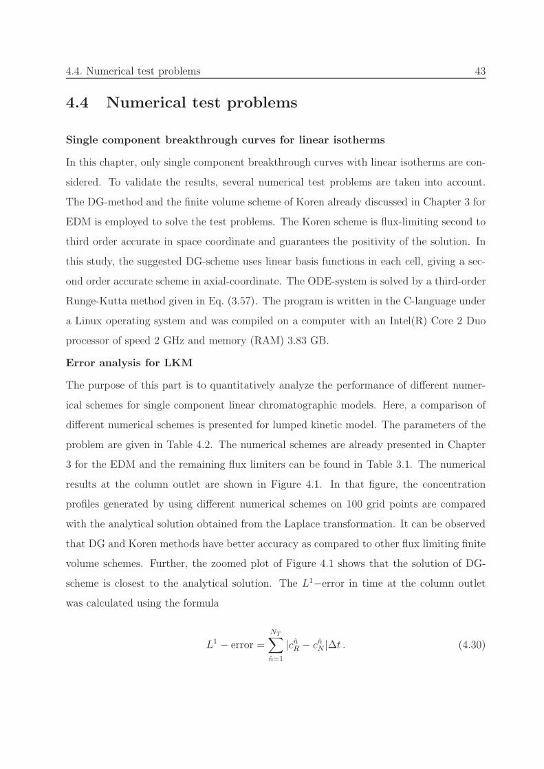
4.4. Numerical test problems 43
4.4 Numerical test problems
Single component breakthrough curves for linear isotherms
In this chapter, only single component breakthrough curves with linear isotherms are con-
sidered. To validate the results, several numerical test problems are taken into account.
The DG-method and the finite volume scheme of Koren already discussed in Chapter 3 for
EDM is employed to solve the test problems. The Koren scheme is flux-limiting second to
third order accurate in space coordinate and guarantees the positivity of the solution. In
this study, the suggested DG-scheme uses linear basis functions in each cell, giving a sec-
ond order accurate scheme in axial-coordinate. The ODE-system is solved by a third-order
Runge-Kutta method given in Eq. (3.57). The program is written in the C-language under
a Linux operating system and was compiled on a computer with an Intel(R) Core 2 Duo
processor of speed 2 GHz and memory (RAM) 3.83 GB.
Error analysis for LKM
The purpose of this part is to quantitatively analyze the performance of different numer-
ical schemes for single component linear chromatographic models. Here, a comparison of
different numerical schemes is presented for lumped kinetic model. The parameters of the
problem are given in Table 4.2. The numerical schemes are already presented in Chapter
3 for the EDM and the remaining flux limiters can be found in Table 3.1. The numerical
results at the column outlet are shown in Figure 4.1. In that figure, the concentration
profiles generated by using different numerical schemes on 100 grid points are compared
with the analytical solution obtained from the Laplace transformation. It can be observed
that DG and Koren methods have better accuracy as compared to other flux limiting finite
volume schemes. Further, the zoomed plot of Figure 4.1 shows that the solution of DG-
scheme is closest to the analytical solution. The L1−error in time at the column outlet
was calculated using the formula
L1 − error =
NT∑
n=1
|cnR − cnN |∆t . (4.30)

44 Chapter 4. Analytical Solution and Moment Analysis for Linear Models
The relative error can be defined as
relative error =
NT∑
n=1
|cnR − cnN |
NT∑
n=1
|cnR|
∆t , (4.31)
where cnR denotes the Laplace solution at the column outlet for time tn and cnN represents
the corresponding numerical solution. Moreover, NT denotes the total number of time
steps and ∆t represents the time step size. Comparisons of L1−errors, relative errors and
computational times of schemes are given in Tables 4.3 and 4.4 for 50 and 100 grid points,
respectively. It can be observed that the DG-scheme produces small errors compared to
the other schemes for both 50 and 100 grid cells, but efficiency (or CPU time) of the Koren
scheme is better than the other schemes for both numbers of grid points. It can be noticed
that relative errors of the DG and Koren schemes are very low for 100 grid points. For that
reason, to achieve acceptable accuracy, 100 mesh points are chosen for further numerical
simulations discussed in this chapter. On the basis of these results, one can conclude that
the DG and Koren methods are optimal choices to approximate chromatographic models.
Therefore, we are relying on the results of the DG scheme for the remaining problems of
this chapter.
Dispersion and mass transfer effects
In this problem, both the single component EDM and LKM models are considered and
compared. The parameters used to solve the model equations are taken from [53] and
are given in Table 4.2. Figure 4.2 (top: left) depicts the dispersion effects of EDM by
considering different values of Dapp or characteristic times τD. It demonstrates that smaller
values of Dapp produce steeper fronts. Figure 4.2 (top: right), shows similar dispersion
effects by varying D as described by the LKM keeping τC = 10 s and τMT = 0.01 s
(k = 100 1/s, τ2 = 103) fixed. The similarity with the corresponding figure for the EDM
is due to the relative large value for k. In Figure 4.2 (bottom: left), different values of the
mass transfer coefficients k for fixed D = 10−5 m2/s (Pe = 104) and τC = 10 s are used for
the LKM. This figure shows that increasing values of k has a similar effects as produced by
decreasing D. In Figure 4.2 (bottom: right), dispersion coefficient D = 10−3 m2/s (Pe =

4.4. Numerical test problems 45
Table 4.2: Parameters for Section 4.4.
Parameters valuesColumn length L = 1.0 m
Porosity ǫ = 0.4Interstitial velocity u = 0.1 m/sCharacteristic time τC = 10 s
Dispersion coefficient for EDM Dapp = 10−4 m2/sPeclet no for EDM τ1 = Pe = 103
Characteristic time for EDM τD = 0.01 sDispersion coefficient for LKM D = 10−5 m2/s
Peclet no for LKM τ1 = Pe = 104
Characteristic time for LKM τD = 0.001 sMass transfer coefficient k = 100 1/s
Characteristic time τMT = 0.01 sDimensionless number τ2 = 103
Concentration at inlet c1,0 = 1.0 g/lAdsorption equilibrium constant a = 0.85
Table 4.3: Errors and CPU times at 50 grid points.
Limiter L1−error Relative error CPU (s)DG Scheme 0.4011 0.0100 5.86
Koren 0.5155 0.0137 4.90Van Leer 0.9324 0.0248 8.26Superbee 1.0732 0.0286 9.34
MC 0.9762 0.0260 8.82
102) is taken into consideration for different values of k. It is evident that even for a large
magnitude of the mass transfer coefficient k, sharp fronts are not possible due to significant
dispersion effects. All trends generated numerically are well-known and realistic for the
adsorption community.
Comparison of analytical and numerical solutions
This part focuses on the comparison of analytical and numerical results from the EDM and
the LKM for both Dirichlet and Danckwerts boundary conditions. In Figure 4.3 (left), the
exact solution obtained for the EDM with Dirichlet boundary conditions is compared with
the numerical Laplace inversion and DG-scheme results. Good agreement of these profiles

46 Chapter 4. Analytical Solution and Moment Analysis for Linear Models
0 0.2 0.4 0.6 0.8 1 1.2 1.4 1.60
0.2
0.4
0.6
0.8
1
1.2
t /µ1
c [g
/l]
Laplace solutionDG−schemeKoren methodVan LeerSuperbeeMC method
0.9 1 1.10
0.2
0.4
0.6
0.8
1
Figure 4.1: Breakthrough curves (BTC) at x = 1. Comparison of different numericalschemes for LKM (c.f. Eq. (4.14) & Eq. (4.25)) with τC = 10 s, τD = 0.01 s (D =10−5 m2/s or τ1 = Pe = 1000) and τMT = 0.01 s (k = 100 1/s or τ2 = 103).
Table 4.4: Errors and CPU times at 100 grid points.
Limiter L1−error Relative error CPU (s)DG Scheme 0.0139 3.71× 10⁻⁴ 8.46
Koren 0.0153 4.08× 10⁻⁴ 7.82Van Leer 0.2255 0.0060 14.90Superbee 0.2966 0.0079 17.73
MC 0.2477 0.0066 14.96
verify the accuracy of numerical Laplace inversion and the proposed numerical scheme.
Moreover, the numerical Laplace inversion technique is found to be a reliable method to
solve such model problems and will be used below in the subsequent case studies. In Figure
4.3 (right), the results of the DG method for the LKM and Dirichlet boundary conditions
are compared with the numerical Laplace inversion solution. No analytical back transform
solution was available for the LKM using Dirichlet boundary conditions. Figures 4.4 (left)
and (right) validate the results of numerical Laplace inversion and the DG-scheme for the
EDM and LKM with Danckwerts boundary conditions, respectively. These profiles show
the high precision of the numerical Laplace inversion technique and the suggested numerical
scheme. Thus, it can also be concluded that the considered numerical Laplace inversion
technique is an effective tool for solving these linear models.

4.4. Numerical test problems 47
0 0.2 0.4 0.6 0.8 1 1.2 1.4 1.6−0.2
0
0.2
0.4
0.6
0.8
1
1.2
t /µ1
c [g
/l]
Dapp
=0
Dapp
=10−5
Dapp
=10−4
Dapp
=10−3
EDM
0 0.2 0.4 0.6 0.8 1 1.2 1.4 1.6−0.2
0
0.2
0.4
0.6
0.8
1
1.2
t /µ1
c [g
/l]
k=100
D=0
D=10−5
D=10−4
D=10−3
LKM
0 0.2 0.4 0.6 0.8 1 1.2 1.4 1.6−0.2
0
0.2
0.4
0.6
0.8
1
1.2
t /µ1
c [g
/l]
D=10−5
k=1k=10k=100k=1000
LKM
0 0.2 0.4 0.6 0.8 1 1.2 1.4 1.6−0.2
0
0.2
0.4
0.6
0.8
1
1.2
t /µ1
c [g
/l]
D=10−3
k=1k=10k=100k=1000
LKM
Figure 4.2: BTC at x = 1. Top (left): Dispersion effects as described by EDM keepingτC = 10 s constant and varying τD (or Dapp), top(right): dispersion effects for LKMkeeping τC = 10 s and τMT = 0.01 s (k = 100 1/s or τ2 = 103) constant, and varying τD(or D), bottom (left): mass transfer effects for LKM taking τC = 10 s, τD = 0.001 s (D =10−5 m2/s or τ1 = Pe = 104) and varying τMT (or k), bottom (right): mass transfer effectstaking τC = 10 s, τD = 0.1 s (D = 10−3 m2/s orPe = 102) and varying τMT (or k).

48 Chapter 4. Analytical Solution and Moment Analysis for Linear Models
0 0.2 0.4 0.6 0.8 1 1.2 1.4 1.6−0.2
0
0.2
0.4
0.6
0.8
1
1.2
t /µ1
c [g
/l]
EDM with Dirichlet BCs
Analytical solutionLaplace numerical inversionDG−scheme
0 0.2 0.4 0.6 0.8 1 1.2 1.4 1.6−0.2
0
0.2
0.4
0.6
0.8
1
1.2
t /µ1
c [g
/l]
LKM with Dirichlet BCs
Laplace numerical inversionDG−scheme
Figure 4.3: BTC at x = 1. EDM predictions using Dirichlet boundary conditions (2.31a),left: comparison of analytical solution (c.f. Eq. (4.15)), Laplace numerical inversion andDG-method solutions with τC = 10 s, τD = 0.02 s (Dapp = 2 × 10⁻⁴ m2/s orPe =500). LKM predictions using Dirichlet boundary conditions (2.31a), right: comparisonof Laplace numerical inversion and DG-scheme solutions with τC = 10 s, τD = 0.01 s (D =10−4m2/s orPe = 1000) and τMT = 0.0667 s (k = 15 1/s or τ2 = 150).
0 0.2 0.4 0.6 0.8 1 1.2 1.4 1.6−0.2
0
0.2
0.4
0.6
0.8
1
1.2EDM with Danckwerts BCs
t /µ1
c [g
/l]
Laplace numerical inversionDG−scheme
0 0.2 0.4 0.6 0.8 1 1.2 1.4 1.6−0.2
0
0.2
0.4
0.6
0.8
1
1.2LKM with Danckwerts BCs
t /µ1
c [g
/l]
Laplace numerical inversionDG−scheme
Figure 4.4: BTC at x = 1. EDM predictions using Danckwerts boundary conditions(2.32a), left: comparison of Laplace numerical inversion and DG-method solutions withτC = 10 s, τD = 0.02 s (Dapp = 2 × 10⁻⁴ m2/s orPe = 500). LKM predictions usingDanckwerts boundary conditions (2.32a), right: comparison of Laplace numerical inversionand DG-scheme solutions with τC = 10 s, τD = 0.01 s (D = 10−4m2/s orPe = 1000) andτMT = 0.0667 s (k = 15 1/s or τ2 = 150).

4.4. Numerical test problems 49
0 0.2 0.4 0.6 0.8 1 1.2 1.4 1.60
0.1
0.2
0.3
0.4
0.5
0.6
0.7
0.8
0.9
1
t /µ1
c [g
/l]
Dirichlet BCs with Pe=1Danckwerts BCs with Pe=1Dirichlet BCs with Pe=2Danckwerts BCs with Pe=2Dirichlet BCs with Pe=10Danckwerts BCs with Pe=10
EDM
0 0.2 0.4 0.6 0.8 1 1.2 1.4 1.60
0.1
0.2
0.3
0.4
0.5
0.6
0.7
0.8
0.9
1
t /µ1
c [g
/l]
Dirichlet BCs with Pe=1Danckwerts BCs with Pe=1Dirichlet BCs with Pe=2Danckwerts BCs with Pe=2Dirichlet BCs with Pe=10Danckwerts BCs with Pe=10
LKM
Figure 4.5: BTC at x = 1. Effect of boundary conditions for different values of Pecletnumber. Symbols are used for Dirichlet BCs (2.31a) and solid lines for Danckwerts BCs(2.32a), left: EDM with τC = 10 s, and Pe or τD varies, right: LKM with τC = 10 s,τMT = 0.01 s (k = 100 1/s or τ2 = 103) and Pe or τD varies.
Effect of boundary conditions
This part is concerned with analyzing effects of boundary conditions. For the sake of gener-
ality, the Peclet number, c.f. Eq. (4.8), is taken as parameter, while τ2 = 103 (τMT = 0.01 s)
and τC = 10 s are assumed to be constant for this problem. The results shown in Fig-
ure 4.5 illustrate the importance of using more accurate Danckwerts boundary conditions
for chromatographic model equations, in the case of relatively small Peclet numbers, e.g.
Pe < 10. For such values, there are visible differences between the results obtained by
using Dirichlet and Danckwerts boundary conditions. On the basis of these results, one
can conclude that the implementation of Dirichlet boundary conditions is not adequate for
large dispersion coefficients. For large values of Peclet number (Pe >> 10) or small axial
dispersion coefficients as typically encountered in chromatographic columns well packed
with small particles, there is no difference between Dirichlet and Danckwerts boundary
conditions. The described behavior was observed in the solutions of both EDM and LKM.
Discussion on analytically and numerically determined moments
In this part, the results regarding the theoretical (analytical) and numerical moments are
discussed. The analytical moments are calculated by the formulas presented in Table 4.1
50 Chapter 4. Analytical Solution and Moment Analysis for Linear Models
and in Appendix A. In this work, only step inputs are taken into account. In contrast
to Eq. (4.29), the formulas given below use derivatives to approximate the moments and
transform the step response to a pulse response which is the requirement for finite results of
numerical integration. The simulated moments are obtained from our proposed numerical
methods by using the following formulas for the first normalized, second central and third
central moments, respectively:
µ1 =
∫∞
0dC(x=1,t)
dttdt
∫∞
0dC(x=1,t)
dtdt
, µ′
2 =
∫∞
0dC(x=1,t)
dt(t− µ1)
2dt∫∞
0dC(x=1,t)
dtdt
, µ′
3 =
∫∞
0dC(x=1,t)
dt(t− µ1)
3dt∫∞
0dC(x=1,t)
dtdt
.
(4.32)
The trapezoidal rule is applied to approximate the integrals in Eq. (4.32) using C(x = 1, t)
which are obtained by using the proposed numerical scheme. The quantitative comparison
of first moment or (retention time) over the flow rate u for the EDM, LKM and the
analytical formula (c.f. Table 4.1) can be seen in Figure 4.6 (left). The results are in good
agreement with each other, verify the high precision of our numerical results and reveal
the expected linear trends.
For calculations of second moments µ′
2 and third moments µ′
3, the analytical formulas of
Table 4.1 are used.
Matching µ′
2EDM and µ′
2LKM for the Dirichlet boundary conditions generates the following
relationship between Dapp, D and k.
Dapp = D +1
k
(aF (1− ǫ)u2
(1 + aF )2
)
. (4.33)
For a given u, a, F , the above equation can be used to find possible connections between
the kinetic parameters of two models which should provide very similar elution profiles.
For given values of a, F and ǫ (c.f. Table 4.1), along with provided reference values of
u∗ = 0.35 m/s and Dapp = 10−4 m2/s for EDM, D = 5 × 10⁻⁵ m2/s for LKM, we obtain
k = 362 1/s from the formula (4.33). Based on these reference parameters, there is an
infinite number of combinations for k and D. The crossing point mentioned in Figure 4.7
(left) indicates that for this particular value of flow rate u∗, both models produce almost
the same concentration profiles as seen in Figure 4.7 (right). For other than this specific

4.5. Conclusion 51
value of flow rate keeping Dapp, D and k fixed, the results of equilibrium dispersive and
lumped kinetic models deviate from each other because the values of Dapp, D and k are
calculated by using this specific velocity u∗ = 0.35 m/s. This is clearly depicted in Figure
4.7 (right).
The third moment still do not match for both models, even when the second moments are
equalized via Eq. (4.33). This is illustrated in the plot given in Figure 4.8 (left) showing the
third moments µ′3 for different flow rates. In Figure 4.8, the parameters Dapp = 10−3 m2/s
for the EDM and D = 5 × 10⁻⁴ m2/s for the LKM are considered. The value of k in the
LKM was always determined for the specific value of u using Eq. (4.33). A good agreement
between analytical and numerical moments of our proposed numerical scheme guarantees
the high precision of simulation results one more time. It can be observed that EDM
gives large values of µ′3 as compared to LKM. Thus, EDM produces more asymmetry in
the concentration profiles which is illustrated in Figure 4.8 (right). The fronting edge is
steeper and the tailing edge is more disperse for the EDM predictions as a clear indication
of larger asymmetry compared to the LKM predictions (c.f. Figure 4.8 (right)). However,
it is evident that the difference in the profiles of both models are still very small. This
justifies the use of the simpler EDM for linear isotherm involving just one parameter Dapp
as compared to the more complicated LKM which involves two parameters D and k.
4.5 Conclusion
This chapter described analytical and numerical investigations of single component lin-
ear equilibrium dispersive and lumped kinetic models. Two sets of boundary conditions,
namely Dirichlet and Danckwerts conditions were considered. The Laplace transformation
was used as a basic tool to transform the single-component linear sub-model to a linear
ordinary differential equation which is then solved analytically in the Laplace domain. The
inverse numerical Laplace formula was employed to get back the time domain solution due
to the unavailability of an exact solution. A moment analysis of both models was carried
out analytically and numerically for linear isotherms. Good agreement up to third mo-

52 Chapter 4. Analytical Solution and Moment Analysis for Linear Models
0 1 2 3 4 5 6 70
2
4
6
8
10
12
14
16
18
1/u [s/m]
first
mom
ent,
µ 1 [s]
Analytical moments (both EDM and LKM)EDM numerical momentsLKM numerical moments
Figure 4.6: First moments µ1 of EDM and LKM for different flow rates u. For EDM,Eq. (A.6) for analytical & Eq. (4.32) for numerical moments are used, considering Dapp =10−4 m2/s. For LKM, Eq. (A.26) for analytical & Eq. (4.32) for numerical moments areused, considering D = 5× 10⁻⁵ m2/s and k = 30 1/s.
0 10 20 30 40 50 60 700
0.01
0.02
0.03
0.04
0.05
0.06
0.07
0.08
1/u3 [s3/m3]
seco
nd m
omen
ts, µ
’ 2 [s2 ]
Analytical EDM momentsnumerical EDM momentsAnalytical LKM momentsnumerical LKM moments
reference: u*=0.35
0.85 0.9 0.95 1 1.05 1.10
0.2
0.4
0.6
0.8
1
1.2
t /µ1
c [g
/l]
EDM with u*=0.35, m/sLKM with u*=0.35, m/sEDM with u=0.1, m/sLKM with u=0.1, m/s
Figure 4.7: Left: Second moments µ′
2 for both models, analytical versus numerical withDapp = 10−4 m2/s for EDM, D = 5 × 10⁻⁵ m2/s and k = 362 1/s for LKM. Crossingat u∗ = 0.35 m/s. Right: Two predicted breakthrough curves for u∗ = 0.35 m/s andu = 0.1 m/s, respectively.

4.5. Conclusion 53
0 1 2 3 4 5 6 7 8 9 10
x 104
0
2
4
6
8
10
12
14
1/u5 [s5/m5]
third
mom
ents
, µ’ 3 [s
3 ]
Analytical EDM momentsnumerical EDM momentsAnalytical LKM momentsnumerical LKM moments
correspondsto u=0.1, m/s
0.6 0.7 0.8 0.9 1 1.1 1.2 1.3 1.4 1.5 1.60
0.02
0.04
0.06
0.08
0.1
0.12
0.14
t /µ1
dc(x
=1,
t)/d
t
0.6 0.65 0.70
0.005
0.01
EDMLKM
1.35 1.4 1.45 1.50
0.005
0.01
Figure 4.8: Left: Third moments µ′
3. For EDM Dapp = 10−3 m2/s, and for LKM, D =5 × 10⁻⁴ m2/s are used. Moreover, k is adjusted for each u via Eq. (4.33) to match µ
′
2.Danckwerts BCs are taken into account. Right: Illustration of effects of differences inthird moments generated by EDM and LKM for u = 0.1 m/s (corresponding to 1/u5 =105 s5/m5).
ments assures the better accuracy of numerical solutions. The close connection between
EDM and LKM was analyzed for linear isotherms. A concordance formula was derived
and the strength of the simpler EDM was illustrated. On the basis of this result, the
EDM is used to predict the chromatographic profiles in the next chapters of this thesis.
For the numerical solution of the models considered, the DG and the Koren schemes were
applied. The Koren scheme is a flux-limiting scheme in which fluxes are limited by us-
ing a nonlinear minmod limiter. This limiting procedure guarantees the positivity of the
scheme and suppresses the numerical oscillations. The proposed DG-scheme satisfies the
TVB property and gives second order accuracy. The method incorporates the ideas of
numerical fluxes and slope limiters in a very natural way to capture the physically relevant
discontinuities without producing spurious oscillations in their vicinity. The accuracy of
proposed schemes were validated against some flux-limiting finite volume schemes and an-
alytical solutions for linear isotherms. The DG-scheme and the Koren method were found
to be suitable methods for the simulation of linear chromatographic processes in terms of
accuracy and efficiency. Moreover, it seems that the DG-scheme resolves the shocks better

54 Chapter 4. Analytical Solution and Moment Analysis for Linear Models
than the Koren scheme. In the subsequent chapter, numerical schemes are analyzed for
more complicated nonlinear and reactive chromatographic models.

Chapter 5
Numerical Solutions of Linear andNon-Linear Chromatographic Models
In this chapter isothermal non-reactive and reactive liquid chromatographic processes are
numerically investigated. Several test problems are carried out concerning both non-
reactive and reactive liquid chromatographic models under linear and non-linear condi-
tions. For linear models, analytical solution can be derived (c.f. Chapter 4), while for
nonlinear models, only numerical techniques provide solutions. Test Problems are numeri-
cally approximated by using the proposed numerical schemes. The results of the suggested
numerical methods are compared with available analytical solutions and some flux-limiting
finite volume schemes given in the literature. Moreover, the quantitative analysis of se-
lected problems is also presented. The case studies of non-reactive chromatography include
single-component elution, two-component elution, and displacement chromatography on
non-movable (fixed) and movable (counter-current) beds. Afterwards, practical examples
of reactive chromatography are taken into consideration and are compared with the avail-
able analytical as well as experimental results.
The finite volume scheme of Koren [39] and the Runge-Kutta discontinuous Galerkin
method, presented in Chapter 3 for FBCR model, are proposed to numerically approx-
imate the current models. The Koren scheme is a flux-limiting scheme in which fluxes
are limited by using a nonlinear minmod limiter. This limiting procedure guarantees the
positivity of the scheme and hence suppresses the numerical oscillations, usually encoun-
55

56 Chapter 5. Numerical Solutions of Linear and Non-Linear Chromatographic Models
tered in the numerical schemes of second and higher orders. In Chapter 3, the scheme was
shown to be second to third order accurate in space analytically. Therefore, a third order
accurate ordinary differential equation (ODE) solver is needed to make the scheme third
order accurate in space and time.
The Runge-Kutta discontinuous Galerkin method [9, 10, 35] is locally conservative, stable,
and high order accurate. The scheme is second order accurate in the axial coordinate and
satisfy the total variation boundedness (TVB) property. In contrast to high order FDMs
and FVMs, the DG-methods require a simple treatment of the boundary conditions to
achieve high order accuracy uniformly. These methods incorporate the idea of numerical
fluxes and slope limiters in a very natural way to avoid spurious oscillations in the re-
gion of strong variations. The DG-methods can be efficiently applied to partial differential
equations (PDEs) of all kinds, including equations whose type changes within the compu-
tational domain. For the first time, these schemes are applied to chromatographic models
in this dissertation.
Several numerical test problems are carried out. For quantitative analysis and validation,
the results of DG-scheme are compared with some flux-limiting finite volume schemes. In
all numerical test problems, linear basis functions are used in each cell, giving a second
order accurate DG-scheme in the axial-coordinate. The ODEs-system was solved by a
third-order Runge-Kutta method given by Eq. (3.57). Once again, the program is written
in the C-language under a Linux operating system and was compiled on a computer with
an Intel(R) Core 2 Duo processor of speed 2 GHz and memory (RAM) 3.83 GB.
5.1 Numerical test problems
In this section the proposed numerical schemes are applied to simulate different chromato-
graphic elution, such as non-reactive single component elution, non-reactive binary elution,
three component elution and four component reactive elution.

5.1. Numerical test problems 57
5.1.1 Non-reactive single-component elution
Here, we give two case studies with linear and nonlinear isotherms, respectively.
Case 1: Linear isotherm: quantitative analysis of the numerical schemes
The purpose of this case study is to quantitatively analyze the performance of the DG-
scheme and different flux-limiting schemes discussed in Chapter 3. For the numerical
simulation, the FBCR model Eq. (3.1) is considered with a linear isotherm q∗ = ac and
the source term Q(t, z, c) is set equal to zero. It is assumed that the column is partially
pre-loaded in the region z = [0.2, 0.4] by a sinusoidal profile. Thus, we assume the following
initial and boundary conditions
c(0, z) =
sin(π(z − 0.2)/0.2) , 0.2 ≤ z ≤ 0.4 ,0, otherwise
(5.1)
with left boundary condition c(0, t) = 0. The analytical solution for this problem is given
as, e.g. [39],
c(t, z) = 0.5 real (iep[erf(α)− erf(β)]) , (5.2)
where, erf represents the error function and
p = −0.5Dappt( π
0.2
)2
+ iπ
0.2(0.2− z − 0.5t) , (5.3)
α =−0.2 + z − 0.5t
2√0.5Dappt
− iπ
√0.5Dappt
0.2, (5.4)
β =−0.4 + z − 0.5t
2√0.5Dappt
− iπ
√0.5Dappt
0.2. (5.5)
The column length L = 1 cm, a = 1, u = 1 cm/min, ǫ = 0.5, and the simulation time is
0.6min. The L1-errors in the axial-coordinate at the last simulation time is calculated by
using the following formula.
L1-error =N∑
j=1
|cjexact − cjnumeric|∆z , (5.6)
where cjexact denotes the exact solution at the midpoint of each discrete cell and cjnumeric
represents the corresponding numerical solution at the final simulation time. Moreover, N
denotes the number of discretization points and ∆z represents the axial step size.

58 Chapter 5. Numerical Solutions of Linear and Non-Linear Chromatographic Models
Table 5.1 gives a comparison of the L1-errors of different numerical schemes using 100 grid
points and for different values of the dispersion coefficients Dapp. It can be observed that
the DG-scheme gives less errors as compared to the flux-limiting finite volume schemes.
Moreover, the errors produced by the Koren scheme are also less at low computational
cost. Note that the DG-scheme used in this work has second order accuracy, while the
Koren scheme is second to third order accurate. Table 5.2 displays the L1-errors and the
experimental order of convergence (EOC) of the DG-scheme at different grid points and
for different values of Dapp. The EOC of the DG-method is approximately second order,
see Table 5.2. The DG-scheme is more effective for the convection dominated problems
where the dispersion coefficient is very small, for example Dapp = 2 × 10⁻⁵ m2/s. Table
5.3 presents the L1-errors and the EOC of the Koren scheme at different mesh points
for different values of Dapp. The table shows that this flux-limiting scheme is second to
third order accurate. The scheme is third order accurate for the convection dominated
equilibrium dispersive models with influential dispersion coefficient, for example Dapp =
2 × 10⁻³ m2/s, while the scheme is second order accurate when the dispersion coefficient
tends to zero. In other words, by varying the number of grid points, the transition rate
from second to third order slowdowns as the dispersion coefficient tends to zero, see Table
5.3. The same trends were also observed by Koren [39]. Finally, Tables 5.4 and 5.5 show
the EOC of different numerical schemes for Dapp = 0.002 m2/s and Dapp = 2× 10⁻⁵ m2/s,
respectively. It can be observed that the Koren scheme gives a better EOC as compared
to other schemes for Dapp = 0.002 m2/s. The DG-scheme provides a comparatively better
EOC for Dapp = 2 × 10⁻⁵ m2/s. In addition, the EOC of other schemes for Dapp =
0.002 m2/s is larger than the DG-method, but the results of the DG-scheme seems to be
slightly closer to the exact solution.
The left plot in Figure 5.1 shows a comparison of different schemes using 50 gird points.
For 50 grid points or less, the Superbee limiter gives the most resolved solution. However,
over-predictions were observed in the solution for grid point numbers above 50. This
limiter applies minimum limiting and maximum steepening. Therefore, it suffers from
excessive sharpening of slopes which results in over-predictions in the solution as depicted

5.1. Numerical test problems 59
Table 5.1: Section 5.1.1 (Linear isotherm): L1-errors and CPU times of schemes at 100mesh points considering different dispersion coefficients Dapp [m2/s]. Parameters are givenin text.
Limiter L1−errors CPU (s)Dapp 0.002 0.0002 2× 10⁻⁵ 2× 10⁻⁶ 0.002
First order 0.04021 0.05303 0.06547 0.05486 0.43DG 0.0009 0.0018 0.0028 0.0030 0.64
Koren 0.00083 0.00278 0.00405 0.00416 0.56van Leer 0.00271 0.00574 0.00675 0.00680 0.56Superbee 0.00336 0.00379 0.00460 0.00475 0.88Minmod 0.00619 0.01079 0.01175 0.01180 1.45MC 0.00227 0.00419 0.00499 0.00503 0.62
Table 5.2: Section 5.1.1 (Linear isotherm): L1-errors and EOC of the DG scheme consid-ering different mesh points N .
N Dapp = 0.002m2/s Dapp = 0.0002m2/s Dapp = 0.00002m2/sL1-errors EOC L1-errors EOC L1-errors EOC
50 0.0028 0.0062 0.0090100 9.31× 10⁻⁴ 1.60 0.0018 1.78 0.0028 1.68200 3.38× 10⁻⁴ 1.46 2.69× 10⁻⁴ 2.73 6.40× 10⁻⁴ 2.13400 1.07× 10⁻⁴ 1.66 6.94× 10⁻⁵ 1.96 1.34× 10⁻⁴ 2.26800 3.05× 10⁻⁵ 1.81 2.24× 10⁻⁵ 1.63 2.43× 10⁻⁵ 2.47
in the right zoomed plot of Figure 5.1. For that reason, more errors were produced by the
Superbee limiter and the convergence rate is very low in Tables 5.1 and 5.5, respectively.
Moreover, the computational cost for the Superbee limiter is higher than the other schemes.
The backward difference method takes the minimum computational time but gives a very
diffusive solution which is far away from the analytical solution. The computational cost
of the van Leer limiter is comparable to the DG and Koren schemes, however its solution
is less resolved. The remaining two limiters have a higher computational cost and lower
accuracy. From the above observations, one can conclude that the DG and Koren schemes
are better choices for solving linear chromatographic models.

60 Chapter 5. Numerical Solutions of Linear and Non-Linear Chromatographic Models
Table 5.3: Section 5.1.1 (Linear isotherm): L1-errors and EOC of the Koren scheme.
N Dapp = 0.002m2/s Dapp = 0.0002m2/s Dapp = 0.00002m2/sL1-error EOC L1-error EOC L1-error EOC
50 0.0065 0.0107 0.0114100 8.31× 10⁻⁴ 2.97 0.0028 1.93 0.004 1.51200 1.02× 10⁻⁴ 3.03 5.64× 10⁻⁴ 2.30 0.0011 1.86400 1.15× 10⁻⁵ 3.15 9.76× 10⁻⁵ 2.53 2.90× 10⁻⁴ 1.93800 1.98× 10⁻⁶ 2.53 1.32× 10⁻⁵ 2.89 6.21× 10⁻⁵ 2.20
Table 5.4: Section 5.1.1 (Linear isotherm): EOC of schemes for Dapp = 0.002 m2/s.
Mesh points N Koren DG van Leer Superbee Minmood MC50100 2.97 1.60 2.08 0.67 1.81 1.92200 3.03 1.46 2.06 1.34 1.99 1.93400 3.15 1.66 2.04 1.86 2.03 1.98800 2.53 1.81 2.02 1.97 2.02 1.99
Table 5.5: Section 5.1.1 (Linear isotherm): EOC of schemes for Dapp = 2× 10⁻⁵ m2/s.
Mesh points N Koren DG van Leer Superbee Minmood MC50100 1.51 1.68 1.52 0.69 1.52 1.45200 1.86 2.13 1.54 1.54 1.14 1.65400 1.93 2.26 1.67 1.67 1.43 1.49800 2.20 2.47 1.70 1.13 1.52 1.52
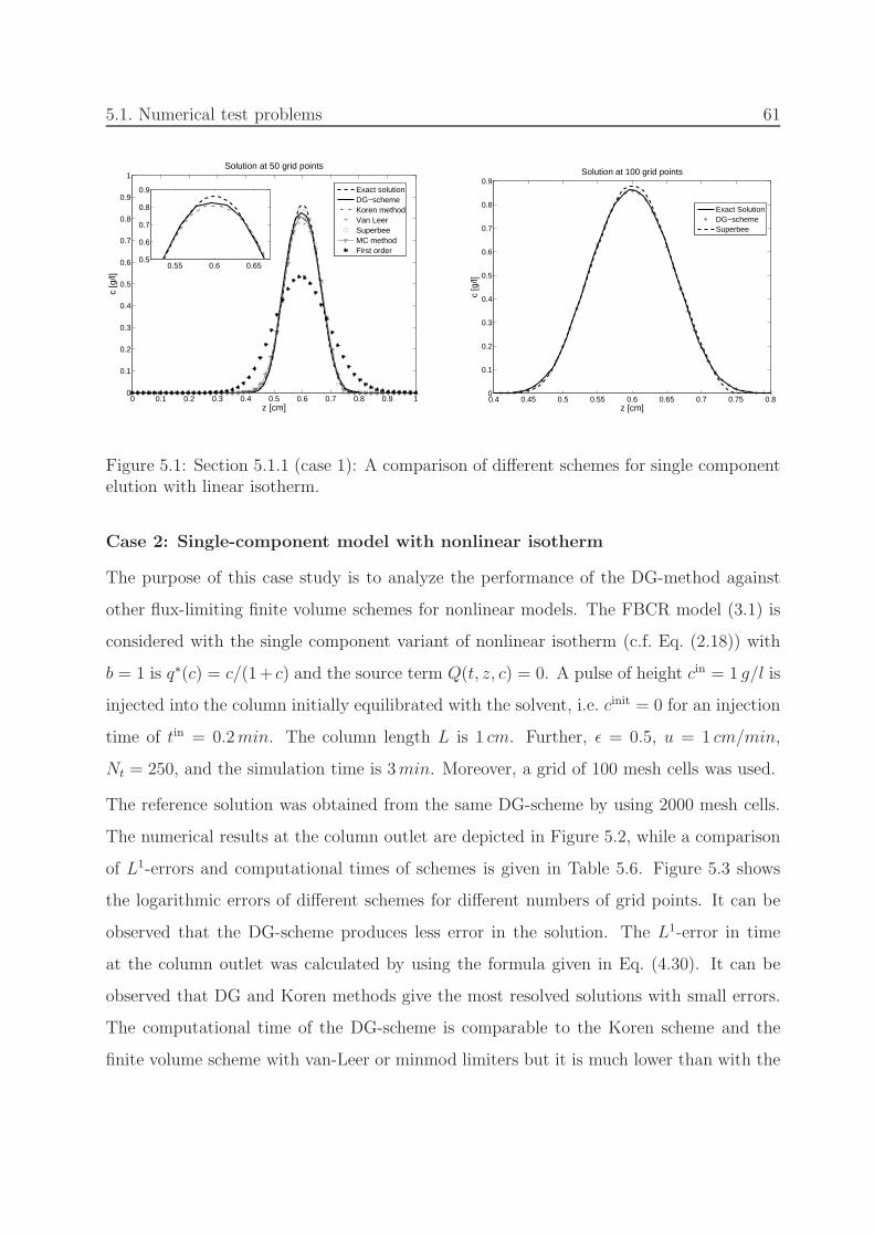
5.1. Numerical test problems 61
0 0.1 0.2 0.3 0.4 0.5 0.6 0.7 0.8 0.9 10
0.1
0.2
0.3
0.4
0.5
0.6
0.7
0.8
0.9
1Solution at 50 grid points
z [cm]
c [g
/l]
Exact solutionDG−schemeKoren methodVan LeerSuperbeeMC methodFirst order
0.55 0.6 0.650.5
0.6
0.7
0.8
0.9
0.4 0.45 0.5 0.55 0.6 0.65 0.7 0.75 0.80
0.1
0.2
0.3
0.4
0.5
0.6
0.7
0.8
0.9Solution at 100 grid points
z [cm]
c [g
/l]
Exact SolutionDG−schemeSuperbee
Figure 5.1: Section 5.1.1 (case 1): A comparison of different schemes for single componentelution with linear isotherm.
Case 2: Single-component model with nonlinear isotherm
The purpose of this case study is to analyze the performance of the DG-method against
other flux-limiting finite volume schemes for nonlinear models. The FBCR model (3.1) is
considered with the single component variant of nonlinear isotherm (c.f. Eq. (2.18)) with
b = 1 is q∗(c) = c/(1+ c) and the source term Q(t, z, c) = 0. A pulse of height cin = 1 g/l is
injected into the column initially equilibrated with the solvent, i.e. cinit = 0 for an injection
time of tin = 0.2min. The column length L is 1 cm. Further, ǫ = 0.5, u = 1 cm/min,
Nt = 250, and the simulation time is 3min. Moreover, a grid of 100 mesh cells was used.
The reference solution was obtained from the same DG-scheme by using 2000 mesh cells.
The numerical results at the column outlet are depicted in Figure 5.2, while a comparison
of L1-errors and computational times of schemes is given in Table 5.6. Figure 5.3 shows
the logarithmic errors of different schemes for different numbers of grid points. It can be
observed that the DG-scheme produces less error in the solution. The L1-error in time
at the column outlet was calculated by using the formula given in Eq. (4.30). It can be
observed that DG and Koren methods give the most resolved solutions with small errors.
The computational time of the DG-scheme is comparable to the Koren scheme and the
finite volume scheme with van-Leer or minmod limiters but it is much lower than with the

62 Chapter 5. Numerical Solutions of Linear and Non-Linear Chromatographic Models
Table 5.6: Section 5.1.1 (Nonlinear isotherm): L1-errors and CPU times of schemes.
Limiter L1−errors CPU (s)N = 50 N = 100 N = 200 N = 50 N = 100 N = 200
DG Scheme 0.0186 0.0063 0.0040 0.23 0.50 1.93Koren 0.0497 0.0225 0.0102 0.22 0.42 1.62
van Leer 0.0586 0.0271 0.0124 0.21 0.41 1.54Superbee 0.0582 0.0281 0.0131 0.34 0.61 2.01
MC 0.0589 0.0276 0.0126 0.26 0.32 1.76Minmod 0.0645 0.0287 0.0125 0.22 0.48 1.57
First order 0.1146 0.0724 0.0415 0.12 0.14 0.70
1 1.5 2 2.5 30
0.1
0.2
0.3
0.4
0.5
0.6
c [g
/l]
solution at the column outlet
t [min]
1.4 1.6 1.8 20.2
0.3
0.4
0.5
referenceDGKorenvan LeerSuperbeeMCminmodfirst order
Figure 5.2: Section 5.1.1 (case 2): A comparison of different schemes for single componentwith nonlinear isotherm.
MC and Superbee limiters. The backward difference scheme has minimal computational
time but gives a very diffusive solution which is far away from the reference solution. The
above observations lead us to the conclusion that DG and Koren schemes are better choices
for solving such nonlinear models.
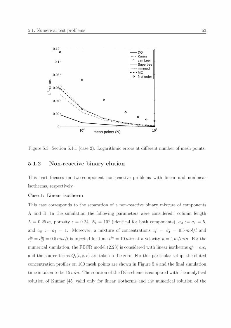
5.1. Numerical test problems 63
102
103
0
0.02
0.04
0.06
0.08
0.1
0.12
mesh points (N)
L1 −er
rors
DGKorenvan LeerSuperbeeminmodMCfirst order
Figure 5.3: Section 5.1.1 (case 2): Logarithmic errors at different number of mesh points.
5.1.2 Non-reactive binary elution
This part focuses on two-component non-reactive problems with linear and nonlinear
isotherms, respectively.
Case 1: Linear isotherm
This case corresponds to the separation of a non-reactive binary mixture of components
A and B. In the simulation the following parameters were considered: column length
L = 0.25m, porosity ǫ = 0.24, Nt = 104 (identical for both components), aA := a1 = 5,
and aB := a2 = 1. Moreover, a mixture of concentrations cin1 = cinA = 0.5mol/l and
cin2 = cinB = 0.5mol/l is injected for time tin = 10min at a velocity u = 1m/min. For the
numerical simulation, the FBCR model (2.23) is considered with linear isotherms q∗i = aici
and the source terms Qi(t, z, c) are taken to be zero. For this particular setup, the eluted
concentration profiles on 100 mesh points are shown in Figure 5.4 and the final simulation
time is taken to be 15min. The solution of the DG-scheme is compared with the analytical
solution of Kumar [45] valid only for linear isotherms and the numerical solution of the

64 Chapter 5. Numerical Solutions of Linear and Non-Linear Chromatographic Models
0 5 10 150
0.1
0.2
0.3
0.4
0.5
0.6
t [min]
c i [mol
/l]
3.5 4 4.5 50
0.1
0.2
0.3
0.4
0.5
analytical
DG
Koren
component Acomponent B
Figure 5.4: Section 5.1.2 (case 1): Two-component elution with linear isotherm.
Koren scheme.
In Figure 5.4, it can be observed that the DG-scheme solution is bit closer to the analytical
solution and gives the position of the discontinuity more correctly compared to the Koren
scheme.
Case 2: Nonlinear isotherm
The propagation of a two component mixture through a column is simulated without
considering reaction or source terms. In the example process considered, the column is
at a constant initial state corresponding to a specific initial composition. A new state
corresponding to a specific feed composition is generated by injecting a new composition
into the column inlet starting at time t = 0. This setup corresponds to a Riemann problem.
Three different fronts usually appear, such as a rarefaction (continuous), a shock wave
and a semi-shock wave. Shocks are discontinuities in the concentration profile due to
experimental conditions. Across the shock wave the concentration increases, therefore the
shock is a compression wave. A rarefaction wave is an expansion wave in time and refers to
the reduction of concentration or opposite to the compression. The EDM, c.f. Eq. (2.21),

5.1. Numerical test problems 65
with generalized Langmuir adsorption isotherm given in Eq. (2.18) is used for modeling
this process as (e.g. in [58])
q∗i = aici/(1 + p1b1c1 + p2b2c2) , i = 1, 2 . (5.7)
For the less retained component the value of ai is smaller as compared to the more retained
component. In the denominator, the values of p1 and p2 can be ±1. The case of p1 = p2 = 1
represents the standard Langmuir isotherm defined in Eq. (5.7) and the case of p1 = p2 =
−1 refers to be anti-Langmuir isotherm. The other two situations are termed as mixed-
Langmuir isotherms. In this study, exclusively a mixed-Langmuir isotherm with p1 = −1
and p2 = 1, is considered.
Mazzoti [58] has analyzed the equilibrium model where Dapp,i = 0 by using the method
of characteristics. Apart from classical composition fronts, such as rarefaction, shock, and
semi-shock waves, non-classical composition fronts and delta-shocks were observed in the
study. Moreover, the analytical (characteristic) solutions of the equilibrium model were
compared with the numerical solutions of the equilibrium-dispersive model for small values
of the axial dispersion coefficient.
In this work, the results of Mazzotti [58] are numerically verified by solving the equilibrium-
dispersive model with our suggested DG and Koren methods. The test problems show that
these schemes preserve narrow peaks in the concentration profiles and give correct locations
of discontinuities. The proposed schemes are efficient, accurate, and produce low numerical
dissipation and dispersion.
A two-component mixture is considered in which component c1 is less retained as compared
to component c2. Here, c1 illustrates an anti-Langmuir and c2 depicts a Langmuir isotherm.
To non-dimensionalize, Eq. (2.21) can be re-written as
∂(ci +1−ǫǫq∗i )
∂t+ u
∂ci∂z
= Dapp,i∂2ci∂z2
, i = 1, 2 . (5.8)
By multiplying the above equation with equilibrium constant bi, we obtain
∂(cibi +1−ǫǫbiq
∗i )
∂t+ u
∂(bici)
∂z= Dapp,i
∂2(bici)
∂z2, i = 1, 2 . (5.9)

66 Chapter 5. Numerical Solutions of Linear and Non-Linear Chromatographic Models
Let µi := cibi represents the ith dimensionless component of liquid phase and νi :=1−ǫǫbiq
∗i
denotes the ith dimensionless component of solid phase. The dimensionless time and axial
coordinates are given as τ = tu/L and x = z/L, where L is the length of the column.
Moreover, τ and x represents the dimensionless time and axial coordinates, respectively.
Finally, the dimensionless diffusion term is given as χi = Dapp,i/Lu. By using the above
definitions, Eq. (5.9) changes to the following dimensionless form, e.g. [58],
∂(µi + vi)
∂τ+
∂µi
∂x= χi
∂2µi
∂x2, i = 1, 2 . (5.10)
Here, vi = aiµi/(1 − µ1 + µ2) and the small parameter χi are the reciprocal of already
defined Peclet numbers (c.f. Eq. (4.4b)).
To apply the numerical schemes, Eq. (5.10) can be written as
(
I+∂v
∂µ
)∂µ
∂τ+
∂µ
∂x= χ
∂2µ
∂x2, (5.11)
where, I represents the identity matrix, µ = (µ1, µ2)T , v = (v1, v2)
T , ∂v/∂µ and χ is
the Jacobian and diagonal matrices, respectively. The above equation is solved by using
current numerical schemes presented in Chapter 3.
To validate the proposed numerical schemes, several numerical test cases are considered.
A typical Riemann problem for Eq. (5.11) consists of an initial state (µF1 , µ
F2 ) assigned to
x ≥ 0 and τ = 0 and an inlet state (µE1 , µ
E2 ) assigned to x = 0 and τ ≥ 0, both separated
by a jump discontinuity. In all test cases of this part, a1 = 1.5, a2 = 3.0, and the mesh
of 200 cells is selected in the axial direction. The number of theoretical plates is chosen
as Nt = 5000, identical for both components, a typical number provided by commercially
available analytical high performance liquid chromatography (HPLC) columns.
Classical solutions: In this case, we have µF1 < µE
2 and µE1 < µF
2 . Such solutions consist
of three states, i.e the inlet state E on the left, the intermediate state I in the middle
defined by the characteristic parameters, and the initial state F on the right, separated
by two transition waves that can be simple waves or shocks. Four test cases, initially
considered in [58], are reproduced with the suggested numerical schemes. Figures 5.7-5.9
show the results. The initial data for these test problems are given in Table 5.7. Figure

5.1. Numerical test problems 67
x [−]
τ [−
]
solution in the physical plane
0 0.2 0.4 0.6 0.8 10
0.5
1
1.5
2
2.5
3
3.5
4
I
F
E
C1
S2
0 1 2 3 4 50
0.05
0.1
0.15
0.2
0.25
τ [−]
µ i [−]
elution profile at the column outlet
S2
I
C1
F E
comp. 1
comp. 2
Figure 5.5: Section 5.1.2 (case 2a): Riemann problem leads to the S2 − C1 solution,a1 = 1.5, a2 = 3.0, inlet state (µE
1 , µE2 ) = (0.1638, 0.1563), initial state (µF
1 , µF2 ) =
(0.0423, 0.1005), and Nt = 5000 (c.f. Eq. (4.4b)).
5.5 gives a S2 − C1 solution, where S2 and C1 represent the left shock wave and the right
simple wave. For validation, the numerical results of the DG-scheme are compared with the
Koren scheme. The Figure 5.6 depicts that the DG-scheme captures sharp discontinuities
better than the Koren scheme. The reference solution was obtained from the DG-scheme
by considering 2000 mesh cells.
In Figure 5.7, the solution has the form C2−S1, where C2 and S1 represent the left simple
wave and right shock wave, respectively. In Figure 5.8, a C2−C1 solution is given. Finally,
Figure 5.9 gives an S2 − S1 solution. It was found that the numerical results of the DG
and Koren schemes agree well with the results published by Mazzoti [58].
Non classical solutions: In this case, the parameter µ2 associated with one state may be
smaller than the parameter µ1 of the other state, and vice versa, see e.g. [58]. The initial
and inlet conditions are given in Table 5.7. Figure 5.10 shows a continuous non-simple
wave transition. This Riemann solution has the form C2 − Ce − C1, where C2, Ce and C1
correspond to a simple left wave, a non-simple wave transition and a right simple wave,
respectively. The results are similar to those presented by [58]. The Riemann problem in
Figure 5.11 leads to the unusual form of a delta shock solution. The existence of a delta
shock has already been realized experimentally [59]. In this case, the concentration shoots

68 Chapter 5. Numerical Solutions of Linear and Non-Linear Chromatographic Models
0 0.5 1 1.5 2 2.5 3 3.5 4 4.50.04
0.06
0.08
0.1
0.12
0.14
0.16
0.18
0.2
0.22two−component elutions at the column outlet
τ [−]
µ i [−]
referenceDG−schemeKoren
comp. 2
comp.1
Figure 5.6: Section 5.1.2 (case 2a): A comparison of the DG and Koren schemes witha1 = 1.5, a2 = 3.0, inlet state (µE
1 , µE2 ) = (0.1638, 0.1563), initial state (µF
1 , µF2 ) =
(0.0423, 0.1005), and Nt = 5000 (c.f. Eq. (4.4b)).
x [−]
τ [−
]
solution in the physical plane
0 0.2 0.4 0.6 0.8 10
0.5
1
1.5
2
2.5
3
3.5
4
EC
2
I
S1
F
0 1 2 3 4 5
0.05
0.1
0.15
0.2
0.25
τ [−]
µ i [−]
elution profile at the column outlet
EIF
comp. 2
comp. 1
C2
S1
Figure 5.7: Section 5.1.2 (case 2b): Riemann problem leads to the C2 − S1 solution,a1 = 1.5, a2 = 3.0, inlet state (µE
1 , µE2 ) = (0.0451, 0.0476), initial state (µF
1 , µF2 ) =
(0.1818, 0.1142), and Nt = 5000 (c.f. Eq. (4.4b)).

5.1. Numerical test problems 69
x [−]
τ [−
]
solution in the physical plane
0 0.2 0.4 0.6 0.8 10
0.5
1
1.5
2
2.5
3
3.5
4
C2
I
C1
F
E
0 1 2 3 4 50
0.05
0.1
0.15
0.2
0.25
0.3
0.35
τ [−]µ i [−
]
elution profile at the column outlet
I
E
F
C2C
1
comp. 2
comp. 1
Figure 5.8: Section 5.1.2 (case 2c): Riemann problem leads to the C2 − C1 solution,a1 = 1.5, a2 = 3.0, inlet state (µE
1 , µE2 ) = (0.1778, 0.0667), initial state (µF
1 , µF2 ) =
(0.0338, 0.2627), and Nt = 5000 (c.f. Eq. (4.4b)).
Table 5.7: Section 5.1.2 (case 2): Inlet and initial conditions for classical and non-classicalsolutions.
Case Inlet state (µE1 , µ
E2 ) Initial state (µF
1 , µF2 )
a (0.1638,0.1563) (0.0423,0.1005)b (0.0451,0.0476) (0.1818,0.1142)c (0.20551,0.05598) (0.0423,0.1005)d (0.1778,0.0667) (0.0338,0.2627)e (0.0317,0.3016) (0.2051,0.0598)f (0,0.2) (0.45,0.0)
up at the jump discontinuity and behaves like a δ-distribution. The concentration µi = bici
and 1 − µ1 + µ2 profiles are presented along the column at different simulation times. It
can be observed that spikes are growing as they travel with a constant speed. Figure 5.12
gives the concentration profiles at the column outlet for different number of theoretical
plates Nt. It can be seen that delta-shock gains height with the increase in Nt, i.e., with
the decrease in dispersion coefficient χ or Dapp.

70 Chapter 5. Numerical Solutions of Linear and Non-Linear Chromatographic Models
x [−]
τ [−
]
solution in the physical plane
0 0.2 0.4 0.6 0.8 10
0.5
1
1.5
2
2.5
3
3.5
4
E
F
I
S1
S2
0 1 2 3 4 50
0.05
0.1
0.15
0.2
0.25
0.3
0.35
0.4
τ [−]µ i [−
]
elution profile at the column outlet
S1
F E
I
S2
comp. 2
comp.1
Figure 5.9: Section 5.1.2 (case 2d): Riemann problem leads to the C2 − C1 solution,a1 = 1.5, a2 = 3.0, inlet state (µE
1 , µE2 ) = (0.0317, 0.3016), initial state (µF
1 , µF2 ) =
(0.2051, 0.0598), and Nt = 5000 (c.f. Eq. (4.4b)).
x [−]
τ [−
]
solution in the physical plane
0 0.2 0.4 0.6 0.8 10
1
2
3
4
5
6
Ce
C1
C2
E
F
0 1 2 3 4 5 6 70
0.1
0.2
0.3
0.4
0.5
τ [−]
µ i [−]
elution profile at the column outlet
F
comp. 1 C2
Ce
E
C1
comp. 2
Figure 5.10: Section 5.1.2 (case 2e): Riemann problem leads to the S2 − S1 solution,a1 = 1.5, a2 = 3.0, inlet state (µA
1 , µA2 ) = (0.4211, 0.0058), initial state (µB
1 , µB2 ) =
(0.0338, 0.2627), and Nt = 5000 (c.f. Eq. (4.4b)).

5.1. Numerical test problems 71
0 0.2 0.4 0.6 0.8 10
0.5
1
1.5
2
2.5
3
3.5
4
4.5
5
x [−]
µ i [−]
comp. 1comp. 2
τ=3.0
τ=2.5
τ=2.0
τ=1.5
τ=0.5τ=1.0
τ=3.5
0 0.2 0.4 0.6 0.8 10
0.5
1
1.5
2
2.5
3
x [−]
1−µ 1+
µ 2
τ=1.5
τ=2.5τ=3.0
τ=1.0
τ=0.5
τ=2.0
τ=3.5
Figure 5.11: Section 5.1.2 (case 2f): µi = bici and 1 − µ1 + µ2 profiles producing delta-shocks along the column, a1 = 1.5, a2 = 3.0, inlet state (µE
1 , µE2 ) = (0.0, 0.2), initial state
(µF1 , µ
F2 ) = (0.45, 0.0), and Nt = 5000 (c.f. Eq. (4.4b)).
3.6 3.65 3.7 3.750
0.5
1
1.5
2
2.5
3
τ [−]
µ 1 [−]
Nt=10
Nt=102
Nt=103
Nt=104
Nt=105
3.6 3.65 3.7 3.750
0.5
1
1.5
2
2.5
3
3.5
4
4.5
5
τ [−]
µ 2 [−]
Nt=10
Nt=102
Nt=103
Nt=104
Nt=105
Figure 5.12: Section 5.1.2 (case 2f): Delta-shocks for different number of theoretical plateswith a1 = 1.5, a2 = 3.0, inlet state (µE
1 , µE2 ) = (0.0, 0.2), initial state (µF
1 , µF2 ) = (0.45, 0.0).

72 Chapter 5. Numerical Solutions of Linear and Non-Linear Chromatographic Models
5.1.3 Three-component elution
This section consists of three different case studies, such as a reaction C A+B with
linear isotherms, nonlinear displacement chromatography in a (fixed) bed, and displacement
chromatography using a moving bed in counter-current direction.
Case 1: Reaction of the type C A+B with linear adsorption isotherm
In such a reaction, only reactant C is injected to the initially unloaded column, while
components A and B are reaction products. Concentration profiles of A and B are detected
at the column outlet. The FBCR model (2.23) with linear adsorption isotherms q∗i = aici is
considered. Based on conventional laws, the reaction rate can be written by the following
equation [91]
Qi(t, z, c) = νir, where r = khet(q∗C −q∗Aq
∗B
Kheteq
) . (5.12)
Here q∗1 := q∗C , q∗2 := q∗A, and q∗3 := q∗B represent the adsorption isotherms of each compo-
nent, and the sign of the stoichiometric coefficient ν1 := νC is negative, while the signs of
ν2 := νA and ν3 := νB are positive. The heterogeneous equilibrium constant Kheteq cannot be
determined experimentally. For a linear adsorption isotherms, considered here, the chemi-
cal equilibrium constant of the heterogeneously catalyzed reaction Kheteq can be written in
terms of the solid-phase concentrations and the equilibrium constant of the homogeneous
reaction Khomeq as
Kheteq = Khom
eq
aAaBaC
. (5.13)
Substitution of Eq. (5.13) into Eq. (5.12) gives
r = khetaC(cC −cAcBKhom
eq
). (5.14)
In this test problem, the parameters are taken from Tien [92]. Here we take the column
length L = 0.25m, porosity ǫ = 0.25, Nt = 104 (identical for all components), Khomeq = 0.5,
khet = 5000min−1, aC = 3, aA = 5, and aB = 1. Moreover, concentration of reactant C, i.e.
cinC = 0.5mol/l, is injected for 10 min with fluid velocity u = 1m/min. The corresponding

5.1. Numerical test problems 73
concentration profiles of cC , cA and cB are shown in Figure 5.13 (left) at 100 mesh cells.
It can be seen that the DG-scheme resolves the discontinuous profiles better with their
correct position compared to the Koren-scheme. These results are in good agreement
with experimental observations of [92]. Outlet concentration profiles can be conveniently
represented in the so-called hodograph space, see Figure 5.13 (right). Hodograph plots are
very useful especially for illustrating problems of FBCR dynamics [30]. The hodograph plot
often reflects the dynamics of process more clearly than the concentration trajectories. The
following important geometrical condition for total conversion and total separation can be
extracted, “total conversion and total separation in a fixed-bed chromatographic reactor
with pulse injection of the reactant is possible, if the relevant wave solutions through the
origin of the corresponding hodograph plot lie on the pure component axes of the products”
[91]. In this plot the concentrations as dependent variables are plotted against each other.
The vertical thick line P0 − P1 shows the fraction of pure component B, obtained from
the front of the elution profile, whereas the horizontal thick line P0 − P3 represents pure
A, collected from the rear of the elution profile. The other two straight lines P0 − P4
and P0 − P5 refer to Section 5.1.2 (case 1) with linear isotherms. The lines which are
located for the case considered exclusively on the pure component axes (thick lines) prove
the capability to obtain pure components A and B from the rear and front of the elution
profiles, respectively.
Case 2: Non-reactive displacement chromatography with Langmuir isotherm
This case study corresponds to an alternative attractive mode of chromatography, namely
displacement chromatography. Displacement chromatography is a powerful method used
to separate and purify compounds. It can be used to purify metal cations, small organic
molecules, antibiotics, sugars, peptides, proteins, and nucleic acids [23]. This process
follows the idea that one strong component, the displacer, has enough capability to displace
the other components from the stationary phase. In this process a column packed with
a solid material is initially equilibrated with the mobile liquid phase that has no or less
affinity to the solid phase. The sample mixture is then injected into the column occupying
part of the column inlet. Afterwards, a development agent, the so called displacer, is

74 Chapter 5. Numerical Solutions of Linear and Non-Linear Chromatographic Models
0 5 10 150
0.1
0.2
0.3
0.4
t [min]
c i [mol
/l]
13.5 14 14.5
0
0.1
0.2
0.3
0.4
cC
cA
cB
referenceDGKoren
0 0.1 0.2 0.3 0.4 0.5 0.6 0.70
0.1
0.2
0.3
0.4
0.5
0.6
0.7
cC+c
A
c C+
c B
Hodograph
p0
p4
p1
p3
p5
p2
Figure 5.13: Section 5.1.3 (case 1): 3-component isothermal-reactive elution with linearisotherm. Parameters are given in text.
injected into the column. Note that, the displacer should have stronger affinity to the solid
phase as compared to other components in the sample. For a sufficiently long column and
favorably shaped isotherms, the sample components will ultimately transport along the
column to build highly concentrated separated rectangular zones. The series of such zones
is known as displacement train or an isotachic train [23]. The displacement effect reduces
the tailing and simplifies the sample loading. Due to these characteristics, displacement
chromatography could be eventually more attractive compared to elution in preparative
scale chromatography.
For illustration, two solute samples with concentrations cA and cB and a displacer with
concentration cd are considered. The FBCR model (2.23) is used to simulate the process
by taking the source terms Qi(t, z, c) equal to zero. The Langmuir isotherm, c.f. Eq. (2.18),
q∗i =aici
1 +3∑
i=1
bici
, i = 1, 2, 3 (5.15)
were used. In simulation, the following parameters were considered: column diameter d =
0.357 cm, L = 100 cm, porosity ǫ = 0.5, aA = a1 = 4, aB = a2 = 5, ad = a3 = 6, b1 = 4 l/g,
b2 = 5 l/g, and bd = 1 l/g. Moreover, Nt = 104 (identical for all components), and the
volumetric flow rate at the column inlet was V = 1ml/min (u = 19.98 cm/min). In the

5.1. Numerical test problems 75
first simulation study, a pulse of a mixture containing cinA = cin1 = 1 g/l and cinB = cin2 = 1 g/l
is injected for an injection time tin = 0.1min. Then, a displacer with a concentration
cind = 1 g/l is fed continuously into the column for the rest of the simulation time. As
the displacer pushes the mixture, both components start separating. For a sufficiently
long column in the present study, the sample components will fully separate and build
highly concentrated rectangular zones of individual concentrations. It is to be noted that
component 1 is less retained than component 2 and the displacer is characterized by the
highest adsorbability. The numerical results are shown in Figure 5.15 using 200 mesh
cells. The operating line in Figure 5.14, plotted under equilibrium conditions, verifies
that both components have less affinity as compared to the displacer. Consequently, both
components are resolved into consecutive rectangular zones of pure substances after 50 cm
and at simulation time t = 13min, see Figure 5.15. For the numerical approximation of
displacement chromatographic process, both suggested schemes, namely the DG and Koren
methods produce reliable results. Moreover, Figure 5.16 shows that the DG-scheme gives
a better resolution of the rectangular profiles at the discontinuity compared to the Koren
scheme. Therefore, the DG-scheme will be used to simulate the processes in the next case
studies of this part.
In the second simulation study, the injection concentrations of both components are cin1 =
cin2 = 1 g/l and the displacer has a concentration cind = 0.5 g/l. Figure 5.17 shows the
numerical results at 200 mesh points. Figure 5.14 shows that a line drawn from the origin
intersects the isotherm of the component 2 but not the isotherm of the component 1.
Hence, the component 2 forms an equilibrated rectangular pulse, while the component 1,
which is now moving at higher speed fails to do so. This is depicted in Figure 5.17.
In the third simulation study, we consider cind = 0.1 g/l. For this value of displacer con-
centration the isotherm plots of both components are not intersected by the operating
line. As a result, both components do not form a rectangular isotachic train as shown
in Figure 5.18. The results presented in this section are found in good qualitative agree-
ment with concentration profiles typically attained in experimental studies of displacement
chromatography.

76 Chapter 5. Numerical Solutions of Linear and Non-Linear Chromatographic Models
0 0.1 0.2 0.3 0.4 0.5 0.6 0.7 0.8 0.9 10
0.5
1
1.5
2
2.5
3
ci [g/l]
q* [g
/l]
displacercomp. 1comp. 2
operating lines
Figure 5.14: Section 5.1.3 (case 2): Representation of the operating line.
Case 3: Displacement chromatography on movable (counter-current) beds
Moving bed chromatography is a mode in which two phases of the chromatographic system,
the fluid and the solid phases, flow through the column in opposite directions. It is known to
be a versatile technique for separating binary mixtures since the 1960s [5]. This simulated
moving bed concept is now employed in a wide range of applications in the pharmaceutical,
medical as well as cosmetic industries. In this case Eq. (2.21) is replaced by the following
equation
∂ci∂t
+1− ǫ
ǫ
∂q∗i∂t
+ u∂ci∂z
− vsF∂q∗i∂z
= Dapp,i∂2ci∂z2
, i = 1, 2, 3 . (5.16)
Here, vs represents the speed of solid particles forming the diffusion free moving bed. Under
steady state conditions, the solid and liquid concentrations at the column outlet are related
as, c.f. Figure 5.19,
(q∗i,L − q∗i,0)1− ǫ
ǫ=
u
vs(ci,L − ci,0) (5.17)

5.1. Numerical test problems 77
0 20 40 60 80 1000
0.2
0.4
0.6
0.8
1
z [cm]
c i [g/l]
displacercomponent 2component 1
0 2 4 6 8 10 12 14 16 180
0.05
0.1
0.15
0.2
0.25
0.3
0.35
0.4
0.45
0.5
t [min]
conc
entr
atio
n [g
/l]
40 cm 60 cm 80 cm5 cm 20 cm
Figure 5.15: Section 5.1.3 (case 2): Formation of displacement train, ǫ = 0.5, Nt = 104
(c.f. Eq. (4.4b)), a1 = 4, a2 = 5, ad = 6, b1 = 4 l/g, b2 = 5 l/g, and bd = 1 l/g withcin1 = cin2 = cind = 1 g/l and tin = 0.1 min.

78 Chapter 5. Numerical Solutions of Linear and Non-Linear Chromatographic Models
0 20 40 60 80 1000
0.2
0.4
0.6
0.8
1
z [cm]
c i [g/l]
comp. 1comp. 2displacer
75 76 77 78 790
0.05
0.1
DG Koren
Figure 5.16: Section 5.1.3 (case 2): A comparison of the DG and Koren schemes. Formationof displacement train, ǫ = 0.5, Nt = 104 (c.f. Eq. (4.4b)), a1 = 4, a2 = 5, ad = 6, b1 = 4 l/g,b2 = 5 l/g, and bd = 1 l/g with cin1 = cin2 = cind = 1 g/l and tin = 0.1 min.
with boundary conditions
ci,0 = cini , q∗i,L = q∗ini ,dcidz
∣∣∣∣z=L
= 0 ,dq∗idz
∣∣∣∣z=0
= 0 . (5.18)
Here, cini represents the injection concentration of component i at the left boundary z = 0
and q∗ini denotes the corresponding injected solid concentration at z = L. The initial data
are the same as used in the first simulation of fixed-bed displacement chromatography in
the previous part, i.e. the concentrations of both components are cin1 = cin2 = 1 g/l with
the displacer concentration cind = 1 g/l. The numerical results were obtained by using the
DG-scheme using 200 mesh points.
At the start of the process, the solid phase was fixed vs = 0 and a mixture was injected
followed by the displacer. The components along with the displacer started moving in the
column and approached the right end of the column after approximately 5 minutes, see
top plot in Figure 5.20. The isotachic train is not reached yet. This would require more
time and a longer bed. In order to reach this attractive pattern with the given bed length,
a new concept is considered. At time t = 5min, a movement of the solid bed particles was

5.1. Numerical test problems 79
activated directed in the opposite direction while the fluid velocity u was set to zero keeping
Dapp unchanged. Consequently, all concentration fronts started moving back. It took about
4 minutes to approach the left end of the column, see the middle plot in Figure 5.20. Finally,
the movement of the solid bed was stopped and the fluid velocity was re-activated. As a
result, the pulses started moving in the forward direction for 4 more minutes, see bottom
plot in Figure 5.20. These back and forth movements ultimately separated the mixture to
build concentrated rectangular zones and form the isotachic train in the total simulation
time of 13 minutes for the given column length. Note that, simulation times are the same
for both fixed-bed and moving-bed processes. However, the moving-bed process allows to
separate the same feed mixture with a relatively shorter column as compared to the fixed-
bed process shown in Figure 5.15. In the bottom plot of Figure 5.20, we have also plotted
the equilibrium profiles of the fixed-bed over the equilibrium profiles of the counter-current
bed in order to verify that both processes give the same results. In that figure symbols
are used for the fixed-bed profiles of Figure 5.15 and lines represent the counter-current
bed profiles of Figure 5.20. Thus, the described moving-bed process can be very useful to
separate mixtures which are difficult to separate and require long chromatographic columns.
Currently, no experimental data or computational results are available for validation of the
simulation results of this case study. However, the results of our numerical study appear
to be useful for further investigation of such processes.
5.1.4 Four-component reactive elution
This part contains two reactive chromatographic case studies with linear and nonlinear
isotherms, respectively.
Case 1: Isothermal reaction with linear isotherms
In this final test problem, a reaction of type A+B C+D along with the temperature
influence on the process is investigated. The feed composition and the flow rate of mobile
phase are assumed to be constant. The ester hydrolysis, experimentally studied by Tien
[92] and Mai [56] is considered as a practical example. The general reaction mechanism is
ester+water alcohol +acid. In such a reaction, only the reactant A (ester) is injected into

80 Chapter 5. Numerical Solutions of Linear and Non-Linear Chromatographic Models
0 20 40 60 80 100 120 1400
0.1
0.2
0.3
0.4
0.5
z [cm]
c i [g/l]
displacercomponent 2component 1
0 5 10 15 20 250
0.05
0.1
0.15
0.2
0.25
0.3
0.35
0.4
t [min]
c i [g/l]
5 cm 80 cm50 cm25 cm
Figure 5.17: Section 5.1.3 (case 2): Displacement chromatography, ǫ = 0.5, Nt = 104
(c.f. Eq. (4.4b)), a1 = 4, a2 = 5, ad = 6, b1 = 4 l/g, b2 = 5 l/g, and bd = 1 l/g withcin1 = cin2 = 1 g/l and cind = 0.5 g/l.
0 20 40 60 80 100 120 140 160 180 2000
0.05
0.1
0.15
0.2
0.25
z [cm]
c i [g/l]
component 2component 1
displacer
0 5 10 15 20 25 30 350
0.01
0.02
0.03
0.04
0.05
0.06
0.07
0.08
t [min]
c i [g/l]
10 cm 50 cm 95 cm
Figure 5.18: Section 5.1.3 (case 2): Displacement chromatography, ǫ = 0.5, Nt = 104
(c.f. Eq. (4.4b)), a1 = 4, a2 = 5, ad = 6, b1 = 4 l/g, b2 = 5 l/g, and bd = 1 l/g withcin1 = cin2 = 1 g/l, cind = 0.1 g/l.

5.1. Numerical test problems 81
(1− ǫ)vsq∗i,0
ǫuci,0
(1− ǫ)vsq∗i,L
ǫuci,L
q∗ici
z = Lz = 0
Figure 5.19: A schematic diagram of counter-current adsorption process.
the column initially loaded only with component B (water), while component C (alcohol)
and component D (acid) are reaction products. Concentration profiles of C and D are de-
tected at the column outlet. The parameters of reaction equilibrium, reaction kinetics, and
adsorption isotherms are given in Table 5.8. The flow rate is 0.75ml/min, cinA = 0.5mol/l,
cinB = 0 = cinC = cinD, u = 0.0622m/min, ǫ = 0.24, L = 0.25m. The injection volume is
100µl. Initially, the column is equilibrated with water only, i.e. cinitB = 55.525mol/l and
cinitA = cinitC = cinitD = 0. The FBCR model (2.23) with linear adsorption isotherms, q∗i = aici,
is considered. The reaction rate of the heterogeneously catalyzed ester hydrolysis reactions
is described by
Qi(t, z, c) = νir , where r = khetfor (q
∗Aq
∗B −
q∗Cq∗D
Kheteq
). (5.19)
Here, the signs of the stoichiometric coefficients νA and νB are negative, while the signs of
νC and νD are positive. For linear adsorption isotherms, the chemical equilibrium constant
Kheteq can be written in terms of the solid-phase concentrations constant Khom
eq as
Kheteq = Khom
eq
aCaDaAaB
. (5.20)
Substituting of equation (5.20) in (5.19), we get
r = khetfor aAaB(cAcB −
cCcDKhom
eq
). (5.21)
The eluted concentrations of the reaction products C and D are shown in Figure 5.21 using
200 mesh cells. To further analyze the performance of the chromatographic reactors, the

82 Chapter 5. Numerical Solutions of Linear and Non-Linear Chromatographic Models
0 5 10 15 20 25 30 350
0.2
0.4
0.6
0.8
1
1.2
z [cm]
c i [g/l]
t=5 min
comp.1comp. 2displacer
0 5 10 15 20 25 30 350
0.2
0.4
0.6
0.8
1
1.2
z [cm]
c i [g/l]
t=9 min
comp. 1comp. 2displacer
0 5 10 15 20 25 30 350
0.2
0.4
0.6
0.8
1
1.2
z [cm]
c i [g/l]
t=13 min
comp. 1
comp. 2
displacer
Figure 5.20: Section 5.1.3 (case 3): Displacement chromatography on counter-current bed,ǫ = 0.5, Nt = 104 (c.f. Eq. (4.4b)), a1 = 4, a2 = 5, ad = 6, b1 = 4 l/g, b2 = 5 l/g, andbd = 1 l/g, cin1 = cin2 = cind = 1 g/l and tin = 0.1 min.

5.1. Numerical test problems 83
Table 5.8: Section 5.4: Temperature dependent reaction and adsorption parameters.
Temperature ai Nt khetfor Khom
eq
A B C D [1/min]298K 1.110 1 0.723 0.458 783 5.88× 10⁻³ 0.38308K 1.082 1 0.750 0.452 886 23.5× 10⁻³ 0.48318K 1.038 1 0.768 0.445 996.5 41.6× 10⁻³ 0.44328K 0.993 1 0.782 0.425 104 103 0.45
reaction is considered at four different temperatures. The numerical results of the DG-
scheme are also compared with the experimental data of [92]. Except for the porosity,
other model parameters heavily depend on the temperature of the column as given in
Table 5.8. The plots of Figure 5.21 show that component A was converted completely in
all cases, but the separation of products C and D was significantly improved at higher
temperatures. The peak widths are also reduced significantly at higher temperatures. In
agreement with the course of the Henry constants, Table 5.8, the retention times of the
product D have a tendency to decrease with temperature increase, whereas the retention
times of the product C have the opposite tendency. The numerical results were found in
relative good agreement with experimental data from [92].
Case 2: Isothermal reaction with nonlinear isotherm
To extend the previous case study to the nonlinear isotherms of Eq. (2.18), we considered
L = 0.25m, u = 0.1322m/min. The remaining data are given in Table 5.8 at a temperature
of 318K. As Langmuir isotherm parameters were considered as bA = 3 l/mol, bB = 0,
bC = 2 l/mol, bD = 1 l/mol, while the ai are the same as in the linear case. No experimental
data or analytical results are available for this setup. The numerical results of the DG-
scheme shown in Figure 5.22. The typical behavior caused by nonlinear Langmuir isotherms
is observed.

84 Chapter 5. Numerical Solutions of Linear and Non-Linear Chromatographic Models
0 2 4 6 8 10 12 14 16 180
0.005
0.01
0.015
0.02
0.025
0.03
0.035
0.04
t [min]
c i [mol
/l]
lines: numerical, symbols: experimental
cC
cD
T=298K
0 2 4 6 8 10 12 14 16 180
0.01
0.02
0.03
0.04
0.05
0.06
t [min]
c i [mol
/l]
lines: numerical, symbols: experimental
cC
cD
T=308K
0 2 4 6 8 10 12 14 16 180
0.01
0.02
0.03
0.04
0.05
0.06
0.07
0.08
t [min]
c i [mol
/l]
lines: numerical, symbols: experimental
cC
cD
T=318K
0 2 4 6 8 10 12 14 16 180
0.01
0.02
0.03
0.04
0.05
0.06
0.07
0.08
0.09
0.1
t [min]
c i [mol
/l]
lines: numerical, symbols: experimental
cC
cD
T=328K
Figure 5.21: Section 5.1.4 (case 1): 4-component isothermal-reactive elution at differenttemperatures with linear isotherms.
0 2 4 6 8 10 12 14 16 180
0.01
0.02
0.03
0.04
0.05
0.06
0.07
t [min]
c i [mol
/l]
T=318K and Langmuir isotherm
cC
cD
T=318K
Figure 5.22: Section 5.1.4 (case 2): 4-component isothermal-reactive elution at temperatureT = 318 with nonlinear isotherm.

5.2. Conclusion 85
5.2 Conclusion
In this chapter, the discontinuous Galerkin finite element method and the Koren scheme
were implemented for solving isothermal non-reactive and reactive chromatographic mod-
els. The second to third order accuracy of the Koren scheme in axial-coordinate was verified
analytically and numerically. The scheme is a flux-limiting scheme in which fluxes are lim-
ited by using a nonlinear minmod limiter. This limiting procedure guarantees the positivity
of the scheme and suppresses the numerical oscillations. The DG-scheme presented satisfies
the TVB property and gives second order accuracy. The scheme can be easily extended to
higher orders by using high order basis functions and by employing better slope limiters,
for example reconstruction with the WENO limiters [69]. This method incorporates the
ideas of numerical fluxes and slope limiters in a very natural way to capture the physically
relevant discontinuities without producing spurious oscillations in their vicinity. In contrast
to finite volume schemes, the DG-scheme is well suited to handle complicated geometries
and avoids the extension of the mesh stencil that allows the incorporation of boundary
conditions uniformly. The accuracy of the proposed schemes were validated against other
flux-limiting finite volume schemes available in the literature. The numerical test problems
verify that the suggested DG-scheme gives more resolved solutions than the high resolu-
tion scheme of Koren, especially at sharp discontinuities. However, desirable results can
also be obtained by using the Koren scheme and we conclude that both the DG and Ko-
ren schemes are optimal methods for the numerical approximation of linear and nonlinear
chromatographic models. The focus of this chapter was to simulate the dynamic behavior
of isothermal chromatographic processes. In the subsequent chapter, the numerical scheme
is extended to solve the non-isothermal reactive liquid chromatographic model.

Chapter 6
Thermal Effects in Reactive LiquidChromatography
This chapter is focused on modeling and simulation of non-isothermal reactive liquid chro-
matography. The purpose of this study is to quantify how temperature gradients can
influence conversion and separation in reactive liquid chromatography. Additionally, the
coupling of concentration and thermal fronts are illustrated and key parameters influencing
the reactor performance are identified.
Thermal effects are discussed widely in case of gas phase reactions in solid packings [21, 27,
40, 104, 105]. In reactive liquid chromatography, thermal effects are typically not considered
and modeling of the process assumes that effects of heats of sorption and reaction are
negligible. Only very few contributions considering thermal effects can be found in the
literature [77, 78, 79, 90].
Non-isothermal reactive chromatography can be described by a convection dominated sys-
tem of non-linear convection-diffusion-reaction type partial differential equations and al-
gebraic equations describing thermodynamic and kinetic phenomena. The corresponding
systems have to be solved numerically because analytical solutions cannot be obtained. The
simulation of non-isothermal reactive chromatography is a challenging task for a numerical
scheme due to the nonlinearity of the convection-dominated mass and energy balance equa-
tions and because of stiffness of the reactive source terms. These stiff terms may produce
rapid variations in the solution and can render the numerical methods unstable, unless the
86

6.1. The non-isothermal chromatographic reactor model 87
time step size is sufficiently small. Thus, an efficient and accurate numerical technique is
needed to avoid excessive dissipation, incorrect phase speeds, spurious oscillations, and to
capture sharp discontinuities of the elution profiles. In order to solve the current problem,
a high resolution finite volume scheme, already developed for isothermal chromatography
in this thesis, c.f. Chapter 3, is extended to solve the non-isothermal processes. Finite
volume schemes were already applied in the chromatographic field [16, 34, 51, 60, 103], but
were never implemented for the complex non-isothermal reactive chromatographic model
considered in this work.
In this study, a flux-limiting semi-discrete high resolution finite volume scheme of Koren
[39] is proposed for the numerical approximation of non-isothermal reactive chromato-
graphic models. The scheme discretizes the model in axial-coordinate only, while keeps
the time variable continuous. The suggested scheme was found to be second to third order
accurate analytically and numerically in the previous chapter on equilibrium dispersive
chromatographic models. The scheme gives high order accuracy on coarse grids, resolves
sharp discontinuities, and avoids numerical dispersion [49]. Several challenging case studies
are carried out which elucidate the effect of several sources for non-isothermal behavior.
The numerical results were evaluated critically by performing consistency tests evaluat-
ing both mass and energy balances including considerations of limiting cases, which can
be theoretically predicted. The results prove the accuracy of the numerical scheme and
quantify the relevant thermal effects.
6.1 The non-isothermal chromatographic reactor model
This section focuses on mathematical modeling of non-isothermal chromatographic reac-
tors. Mathematically, the non-isothermal single column chromatographic reactor is similar
to a more frequently studied non-isothermal unsteady-state fixed bed reactor [72, 78]. The
model is based on the following basic assumptions:
1. A permanent equilibrium is assumed between stationary and mobile phases at all
positions of the column.

88 Chapter 6. Thermal Effects in Reactive Liquid Chromatography
2. A single reaction takes place exclusively in the solid phase.
3. There are no radial concentration and temperature gradients in the column and a
one dimensional description is used.
4. Only axial dispersion causes band broadening described by Dapp and λax in the mass
and energy balances, respectively.
5. Compressibility of the mobile phase is negligible.
6. There are no interactions between the solvent (carrier) and the solid phase.
7. There is no heat added or removed from the system except via the inlet and outlet
streams, i.e. adiabatic operation.
The classical mass balance equations of the equilibrium dispersive model for a fixed bed
chromatographic column are given as
(
1 + F∂q∗i∂ci
)∂ci∂t
+ u∂ci∂z
= Dapp,i∂2ci∂z2
+ Fνir , i = 1, 2, · · · , Nc , (6.1)
where F is the phase ratio based on the porosity ǫ ∈]0, 1[ and F = 1−ǫǫ, ci is the concentra-
tion of the i-th component in the fluid phase, q∗i is the solid phase equilibrium concentration
of the i-th component, u represents the constant interstitial velocity of the mobile phase,
Dapp,i represents the axial dispersion coefficient of the i-th component, t is the time, and
z is the axial-coordinate along the column. Moreover, r is the rate of the reaction in the
solid phases, the νi are the corresponding stoichiometric coefficients of components and Nc
represents the total number of components. Note that, the stoichiometric coefficients νi
are negative for reactants and positive for products.
If the enthalpy of mixing is neglected, the energy balance for a differential volume element
in an adiabatic chromatographic reactor becomes
(ρLCLp + FρSCS
p)∂T
∂t+ uρLCL
p
∂T
∂z= λax
∂2T
∂z2+ F
Nc∑
i=1
(−∆HA,i)∂q∗i∂t
+ F (−∆HR)r . (6.2)

6.1. The non-isothermal chromatographic reactor model 89
Here ρ represents the density per unit volume, Cp is the heat capacity, and the superscripts
L and S stands for the liquid and solid phases, respectively. The considered density and heat
capacity are not depending on temperature and composition. Moreover, ∆HA,i denotes the
enthalpy of adsorption for the i-th component and ∆HR represents the enthalpy of reaction.
By using the assumptions of non-dispersive and non-reactive chromatography, the propa-
gation velocities of concentration fronts uic and of the thermal front uT can be estimated
from Eqs. (6.1) and (6.2) as:
uic∼=
u
1 + F∂q∗i∂ci
, uT∼=
u
1 + FρSCS
p
ρLCLp
, i = 1, 2, · · · , Nc . (6.3)
The Eq. (6.3) reveals that the propagation velocities uic depend on the corresponding local
slopes of the adsorption isotherms and that the propagation velocity uT is influenced by
the ratio of the volumetric density times heat capacities of solid and liquid phases. For
weakly adsorbed components or small slopes of isotherm∂q∗i∂ci
and for significantly higher
ratio ofρSCS
p
ρLCLp, the velocities of concentration fronts ui
c are higher than the thermal velocity
uT .
For non-reactive chromatography under non-isothermal conditions, it was shown that the
energy balance can be formulated as the Nc + 1-th equation, analogously to the Nc mass
balance equations [72]. This idea can be extended easily to reactive systems if the heat
of reaction is assumed to be an analogue to the Nc + 1 stoichiometric coefficient, i.e.
νNc+1 = −∆HR. Hereby, the energy balance is formulated in a convenient way with
respect to a reference temperature T ref .
Generally, the computer implementation of dimensionless equations is more convenient to
reduce rounding error. The current system can be transformed into a dimensionless form
by introducing the following dimensionless time and axial coordinates
τ = tu/L , x = z/L (6.4)

90 Chapter 6. Thermal Effects in Reactive Liquid Chromatography
and the new variables
νNc+1 = −∆HR, (6.5a)
cNc+1 = ρLCLp (T − T ref), (6.5b)
q∗Nc+1 = ρSCSp (T − T ref) +
Nc∑
i=1
∆HA,iq∗i . (6.5c)
By using the chain rule and Eqs. (6.4) and (6.5), the Eqs. (6.1) and (6.2) can be lumped
together as a single system of Nc + 1 equations:
(
1 + F∂q∗m∂cm
)∂cm∂τ
+ F
Nc+1∑
l=1l 6=m
∂q∗m∂cl
∂cl∂τ
+∂cm∂x
=1
Pe
∂2cm∂x2
+Lνmu
Fr , (6.6)
where m = 1, 2, · · · , Nc + 1. The dimensionless Peclet number Pe is given as
Pem =
PeM = Lu
Dappif m = 1, 2, · · · , Nc ,
P eE =LuρLCL
p
λaxif m = Nc + 1,
(6.7)
where L is the column length and PeM is equal to two times of the frequently used number
of theoretical plates Nt and assumed to be the same for all components.
Now it is required to define Nc + 1 initial and 2(Nc + 1) boundary conditions to close
the model (6.6). For an initially uniformly equilibrated column, the initial and boundary
conditions for the Nc dimensionless mass balance equations of Eq. (6.6) are given as:
cm(0, x) = cinitm , cm(τ, 0) = cinm(t) +L
Pe
∂cm∂x
∣∣∣∣x=0
,∂cm∂x
∣∣∣∣x=1
= 0 , m = 1, 2, · · · , Nc ,
(6.8a)
and the conditions for the Nc + 1-th dimensionless energy balance equation are given as
cNc+1(0, x) = 0 , cNc+1(τ, 0) = T in +L
Pe
∂cNc+1
∂x
∣∣∣∣x=0
,∂cNc+1
∂x
∣∣∣∣x=1
= 0 , (6.8b)
where cinj , Tinit and T in represent the inlet concentrations, initial temperature and tempera-
ture at the column inlet, respectively. In this work, T in, T init and the reference temperature
T ref are taken to be identical.
In this study, for illustration a simple reversible reaction A B+C is considered and
linear adsorption isotherms are assumed. An inert carrier (solvent), present in excess is

6.2. Formulation of numerical scheme 91
transporting the three components through the column. The amount of solute adsorbed
depends on temperature as described by a van’t Hoff type relation using the enthalpy of
adsorption. In the case of a linear adsorption isotherms, the phase equilibrium relations
for components can be written as
q∗i = aici , i = 1, 2, 3 , (6.9a)
with ai = arefi exp
(−∆HA,i
R
(1
T−
1
T ref
))
, i = 1, 2, 3 . (6.9b)
To describe the reaction rate the standard expression for a reversible reaction is applied
using the solid phase concentrations to define the driving force
r = kfor(T )
(
q∗A −q∗Bq
∗C
K∗eq(T )
)
. (6.10a)
The effect of temperature on the chemical reaction rate kfor(T ) is an exponential function
of the absolute temperature as described by the Arrhenius equation using the activation
energy EA
kfor(T ) = kfor(Tref) exp
(−EA
R
(1
T−
1
T ref
))
. (6.10b)
Chemical equilibrium constants K∗eq(T ) depend on the temperature as given below
d lnK∗eq
dT=
∆HR
RT 2. (6.11a)
After integrating the above equation from T ref to T , we obtain another von’t Hoff expression
K∗eq(T ) = K∗
eq(Tref) exp
(−∆HR
R
(1
T−
1
T ref
))
. (6.11b)
This completes the derivation of the model for the non-isothermal chromatographic reactor.
In the next section the flux-limiting finite volume scheme used to solve the model equations
is presented.
6.2 Formulation of numerical scheme
In this section, the high resolution scheme of Koren [39] is described with respect to this
particular problem. It should be noted that Nc = 4 refers to three species A, B and C and

92 Chapter 6. Thermal Effects in Reactive Liquid Chromatography
the fourth pseudo-component which captures the specifics of the energy equation, cf., Eq.
(6.5b). The Eq. (6.6) can be re-written as
J∂c
∂τ+ u
∂c
∂x= P
∂2c
∂x2+Q , (6.12a)
where, J, c, P and Q are given as
J =
1 + F∂q∗1∂c1
F∂q∗1∂c2
F∂q∗1∂c3
F∂q∗1∂c4
F∂q∗2∂c1
1 + F∂q∗2∂c2
F∂q∗2∂c3
F∂q∗2∂c4
F∂q∗3∂c1
F∂q∗3∂c2
1 + F∂q∗3∂c3
F∂q∗3∂c4
F∂q∗4∂c1
F∂q∗4∂c2
F∂q∗4∂c3
1 + F∂q∗4∂c4
, c =
c1c2c3c4
, (6.12b)
P =
1PeM
0 0 0
0 1PeM
0 0
0 0 1PeM
0
0 0 0 1PeE
, Q = Fr
Lν1u
Lν2u
Lν3u
Lν4u
. (6.12c)
Before applying the proposed numerical scheme to Eq. (6.12), it is required to discretize the
computational domain. Let N represents the number of discretization points and the points
(xj− 12), j ∈ 1, · · · , N + 1 be partitions of the interval [0, 1]. For each j = 1, 2, · · · , N , ∆x
is a constant width of each mesh interval. The xj denote the cell centers, and xj± 12refer
to the cell boundaries. We assign
x1/2 = 0 , xN+1/2 = 1 , xj+1/2 = j ·∆x , for j = 1, 2, · · ·N . (6.13)
Moreover, we have
xj = (xj−1/2 + xj+1/2)/2 and ∆x = xj+1/2 − xj−1/2 =1
N + 1. (6.14)
Let Ωj :=[xj−1/2, xj+1/2
]for j ≥ 1. The cell averaged initial data in each cell are given as
cj(0) =1
∆x
∫
Ωj
cinit(x) dx , for j = 1, 2, · · ·N . (6.15)
By integrating Eq. (6.12a) over the interval Ωj =[xj−1/2, xj+1/2
], we obtain
∫
Ωi
J∂c
∂τdx = −u
(
cj+ 12− cj− 1
2
)
+Pj
[(∂c
∂x
)
j+1/2
−
(∂c
∂x
)
j−1/2
]
+
∫
Ωj
Q dx . (6.16)

6.2. Formulation of numerical scheme 93
In each Ωj , the averaged values of the conservative variables c(t) are given as
cj(t) =1
∆x
∫
Ωj
c(t, x) dx . (6.17)
In Eq. (6.17), cj are cell averaged vectors of concentration components, while in Eq. (6.16),
cj± 12are the vectors at the respective cell boundaries. Similarly, the cell-averaged value
of source term Q can be defined. Moreover, the Jacobian matrix J is calculated at the
cell centroid xj . Therefore, by using Eq. (6.17) in Eq. (6.16), the following semi-discrete
scheme is obtained, for each, j = 1, 2, · · · , N ,
Jjdcjdτ
= −u(
cj+ 12− cj− 1
2
)
+Pj
[(∂c
∂x
)
j+1/2
−
(∂c
∂x
)
j−1/2
]
+Qj . (6.18)
The differential terms of the diffusion part can be approximated as
(∂c
∂x
)
j± 12
= ±
(cj±1 − cj
∆x
)
. (6.19)
The next step is to approximate the values for the convective variables at the cell interfaces
cj± 12, in Eq. (6.18). Hereby, different approximations give different numerical schemes.
First order scheme: In this case, the fluxes are approximated as
cj+ 12= cj , cj− 1
2= cj−1 . (6.20)
This approximation gives a first order accurate scheme in the axial-direction.
High resolution schemes: To achieve higher order accuracy, a piecewise interpolation
polynomial can be used, such as
cj+ 12= cj +
1 + κ
4(cj+1 − cj) +
1− κ
4(cj − cj−1) , κ ∈ [−1, 1] . (6.21)
Similarly, cj− 12can be written as
cj− 12= cj−1 +
1 + κ
4(cj − cj−1) +
1− κ
4(cj−1 − cj−2) , κ ∈ [−1, 1] , (6.22)
where the parameter κ is selected from the interval [−1, 1]. For κ = −1, one gets the second
order accurate fully one-sided upwind scheme, and for κ = 1, the standard second order
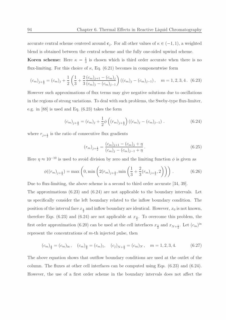
94 Chapter 6. Thermal Effects in Reactive Liquid Chromatography
accurate central scheme centered around cj . For all other values of κ ∈ (−1, 1), a weighted
blend is obtained between the central scheme and the fully one-sided upwind scheme.
Koren scheme: Here κ = 13is chosen which is third order accurate when there is no
flux-limiting. For this choice of κ, Eq. (6.21) becomes in componentwise form
(cm)j+ 12= (cm)j +
1
2
(1
3+
2
3
(cm)j+1 − (cm)j(cm)j − (cm)j−1
)
((cm)j − (cm)j−1) , m = 1, 2, 3, 4 . (6.23)
However such approximations of flux terms may give negative solutions due to oscillations
in the regions of strong variations. To deal with such problems, the Sweby-type flux-limiter,
e.g. in [88] is used and Eq. (6.23) takes the form
(cm)j+ 12= (cm)j +
1
2φ(
(rm)j+ 12
)
((cm)j − (cm)j−1) . (6.24)
where rj+ 12is the ratio of consecutive flux gradients
(rm)j+ 12=
(cm)j+1 − (cm)j + η
(cm)j − (cm)j−1 + η. (6.25)
Here η ≈ 10−10 is used to avoid division by zero and the limiting function φ is given as
φ((rm)j+ 12) = max
(
0,min
(
2(rm)j+ 12,min
(1
3+
2
3(rm)j+ 1
2, 2
)))
. (6.26)
Due to flux-limiting, the above scheme is a second to third order accurate [34, 39].
The approximations (6.23) and (6.24) are not applicable to the boundary intervals. Let
us specifically consider the left boundary related to the inflow boundary condition. The
position of the interval face x 12and inflow boundary are identical. However, x0 is not known,
therefore Eqs. (6.23) and (6.24) are not applicable at x 32. To overcome this problem, the
first order approximation (6.20) can be used at the cell interfaces x 32and xN+ 1
2. Let (cm)
in
represent the concentrations of m-th injected pulse, then
(cm) 12= (cm)in , (cm) 3
2= (cm)1, (cj)N+ 1
2= (cm)N , m = 1, 2, 3, 4. (6.27)
The above equation shows that outflow boundary conditions are used at the outlet of the
column. The fluxes at other cell interfaces can be computed using Eqs. (6.23) and (6.24).
However, the use of a first order scheme in the boundary intervals does not affect the

6.3. Consistency tests for validation 95
global accuracy of the method due to shrinking cell sizes with increasing node numbers.
The efficiency and accuracy of the scheme were thoroughly analyzed in the previous chapter
on isothermal dispersive liquid chromatography.
The above described semi-discrete scheme was programmed in Matlab 7.9.1 software and
the resulting ODE-system was solved by using the built-in Matlab routine ode15s.
6.3 Consistency tests for validation
Currently, not many experimental results are available to quantify non-isothermal reactive
chromatographic processes. Thus, integral consistency tests for mass and energy balance
equations are useful tools to validate numerical results and also the correctness of the
model formulation. Based on such tests, the accuracy of the numerical scheme and the
conservativity of mass and energy balances were evaluated for the considered reversible
chemical reaction A B+C.
6.3.1 Identity of integrated extents of reaction
In a chemical reaction, the changes in mole numbers of the components ni are connected
by the stoichiometry of the reaction. For the considered reversible chemical reaction A
B+C, the integrated extent of reaction ξ should be independent on component and should
follow the subsequent equation
ξ = ninA − nout
A = noutB = nout
C . (6.28)
The single variable ξ describes all the changes in the mole numbers due to the chemical
reaction and nini = cini V
in represents injected moles into the column. In this study, the
inlet concentrations of the products i.e., cinB and cinC were taken to be zero. The symbol V in
denotes the volume injected at the column inlet during the injection time tin.
After solving the PDEs the mole numbers can be calculated at the outlet using the following
equation
nouti = V
∫ t∗
0
ci(t, x = L)dt , i = A,B,C, (6.29)

96 Chapter 6. Thermal Effects in Reactive Liquid Chromatography
where V represents the volumetric flow rate related to u. The above integrals were evalu-
ated for each component using the trapezoidal rule. The integration of the PDEs solution
should be carried sufficiently long to return to the initial state (time t∗).
A standard deviation is calculated for the three values of ξi as
σξ,i[%] = 100×
√∑Nc
i=1(ξi − ξ)2
3, i = A,B,C. (6.30)
Here ξ is the average of ξA, ξB, ξC . This standard deviation should tend to zero if the mass
balances respect stoichiometry.
6.3.2 Integrated energy balance considering the extent of reac-
tion
An energetic evaluation of the process can be made by comparing the enthalpies entering,
∆H in, and leaving, ∆Hout, the system. These enthalpies are
∆H in = ρLcLp V
∫ t∗
0
(T in − T ref)dt , ∆Hout = ρLcLp V
∫ t∗
0
(T (t, x = L)− T ref) dt . (6.31)
For T in = T ref holds ∆H in = 0. In case of a complete adsorption and desorption cycle (t∗
sufficiently long), there will be no overall sorption effect and the following balance equation
can be derived using exclusively the effect of reaction quantified by ∆HR and ξ, e.g. Eq.
(6.30)
∆Hout + (∆HR)ξ = 0 . (6.32)
The fulfillment of Eq. (6.32) is required as a proof of accurate numerical simulations. There
are several sources of numerical errors, such as discretization errors, round off errors, and
errors in the numerical integrations of the outlet profiles, etc. Due to these errors, the right
hand side of Eq. (6.32), called here ∆Herr, might not be exactly zero
∆Herr = ∆Hout + (∆HR)ξ . (6.33)
The smaller the ∆Herr the better is the fulfillment of the joint integral mass and energy
balances. One can expect larger errors in ∆Herr compared to errors in ξ due to the accu-
mulation of all possible errors in this more critical consistency check. A relative percentage

6.4. Demonstrations of thermal effects 97
error in this energy can be given as
EH[%] = 100×
∣∣∣∣
∆Herr
∆HRξ
∣∣∣∣. (6.34)
6.4 Demonstrations of thermal effects
The purpose of this section is to evaluate effects of parameters that influence conversion
and separation in non-isothermal reactive liquid chromatography. Numerical test problems
will explain the coupling between the concentration and thermal fronts in the reactor.
We consider, the reversible reaction AB+C, and linear isotherm with Henry constants
arefA = 1.0, arefB = 0.7 and arefC = 1.3 at reference temperature T ref = 300 K. This means
that the feed component A elutes between the two products B and C. Moreover, a reaction
rate constant kfor(Tref) = 10−4 1/s, a reaction equilibrium constant K∗
eq = 2 mol/l, an
activation energy EA = 60 kJ/mol and density times heat capacities for liquid and solid
phases ρLCLp = ρSCS
p = 4.0 kJ/lK are used for numerical simulations. Further, the column
length is L = 27 cm, the interstitial velocity is u = 0.6240 cm/min, the volumetric flow
rate is V = 0.4980 cm3/min. The phase ratio F = 1.5 corresponds to the external porosity
ǫ = 0.4. A pulse of height cinA = 3 mol/l is injected into the column initially equilibrated
with the solvent, i.e. ciniti = 0 for an injection time tin of 16.68 min corresponding to
a dimensionless injection time τ in of 0.385. In most of the cases, based on preliminary
calculations a final simulation time 174 min is taken into account to assure complete
regeneration. In all test problems, the dimensionless model, Eq. (6.6), is used and the
Koren scheme mostly with 400 mesh cells in axial direction is employed for numerical
simulations. The values for the reaction enthalpy and the adsorption enthalpies were
varied in typical ranges, i.e. ∆HR = [−50, 50] kJ/mol, and ∆HA,i = [−20, 0] kJ/mol.
6.4.1 Trivial limiting cases
At first, some trivial limiting studies are considered for validation.
Case 1: There is no reaction, kfor = 0, and enthalpies of adsorption are negligible, ∆HA,i =
0, in the model Eq. (6.6). Moreover, dispersion effects are ignored by considering both

98 Chapter 6. Thermal Effects in Reactive Liquid Chromatography
Peclet numbers of mass PeM and energy PeE approach to ∞. As a result, reactants would
be not able to convert into the products. The reactant is only transported through the
column and the product components B and C are not formed. The correctly obtained
solution for this particular case is shown in Figure 6.1.
If the enthalpy of reaction is taken to be zero, i.e., ∆HR = 0, then ∆Hout = 0, and no
temperature change can occur as depicted in Figure 6.1 (right).
Case 2: Adiabatic temperature rise
This part evaluates the adiabatic temperature rise. The reactant A is continuously fed with
three different injection concentrations cinA = 3 mol/l, cinA = 6 mol/l and cinA = 12 mol/l
for sufficiently long injection and residence times along with a set of parameters namely,
∆HA,i = 0, ∆HR = −10 kJ/mol, and PeM and PeE approach to∞. The formula describing
the adiabatic temperature rise based on Eqs. (6.1) and (6.2) is
∆Tadabatic =−∆HRc
inA
ρLcLp. (6.35)
For the considered injection concentrations, this formula give the values of ∆Tadabatic as
7.5 K, 15 K and 30 K, respectively. The corresponding temperature profiles together
with selected concentration profiles are shown in Figure 6.2. The figure verifies, that after
complete conversion of the reactant, the predicted temperature profiles indeed attain the
steady maxima and the values of ∆Tadabatic in the figure agree with those obtained from Eq.
(6.35). The slight overshoots in Figure 6.2 are produced by the numerical scheme which
have no physical reason. This completes the discussion of trivial cases.
6.4.2 Non-trivial test problems
Problem 1: Isothermal case:
The purpose of this first study is to analyze the isothermal behavior as well as to quan-
titatively investigate the errors of extent of reaction ξ and conversion. To simulate the
isothermal case, the enthalpies of adsorption, ∆HA,i, and the enthalpy of reaction, ∆HR,
are set equal to zero. Additionally, dispersion effects are neglected by considering both
PeM and PeE approaching ∞. In order to analyze the effect of the adsorption isotherms,

6.4. Demonstrations of thermal effects 99
1 1.5 2 2.5 3 3.5 40
0.5
1
1.5
2
2.5
3
dimensionless time, τ
conc
entr
atio
n [m
ol/l]
1 1.5 2 2.5 3 3.5 4295
296
297
298
299
300
301
302
303
304
305
dimensionless time, τte
mpe
ratu
re [K
]
Figure 6.1: Trivial limiting cases: case 1: ∆HA,i = 0 for i=A,B,C, kfor(Tref) = 0.
1 1.5 2 2.5 3 3.5 4 4.5 5 5.5 6
x 104
295
300
305
310
315
320
325
330
335
time [s]
tem
pera
ture
[K]
cinA
=12 mol/l
cinA
=6 mol/l
cinA
=3 mol/l
1 2 3 4 5 6
x 104
−1
0
1
2
3
4
5
6
7
time [s]
conc
entr
atio
ns [m
ol/l]
concentration transients for cinA
=6 mol/l
A (reactant) B (Product)C (product)
Figure 6.2: Trivial limiting cases: case 2: ∆HA,i = 0 for i=A,B,C, ∆HR = −10 kJ/mol,L = 1.62 m, kfor(T
ref) = 10−4 s−1, left: temperature transients at the column outletfor three inlet concentrations, right: the corresponding concentration transients for cinA =6 mol/l.

100 Chapter 6. Thermal Effects in Reactive Liquid Chromatography
Table 6.1: Problem 1: Isothermal case. Here XA[%] = 100×ninA−nout
A
ninA
.
parameters ξA ξB ξC σξ,i XA ∆Hout
[mol] [mol] [mol] [%] [%] [kJ]ai = 0 -0.0001 −5.7e−27 −1.0675e−10 ≈ 0 -0.0040 0arefi 6= 0 0.0079 0.0080 0.0080 0.0058 31 0
at first the Henry constants ai are put equal to zero for all components, i.e. aA = 0, aB = 0,
and aC = 0. Due to Eq. (6.10a) the reaction rate would also be zero and the reactant A
would not be converted into products and would be just transported along the column.
This behavior can be seen in Figure 6.3 (top). Then we considered the reference Henry
constants in Eq. (6.9) as arefA = 1.0, arefB = 0.7, and arefB = 1.3. The obtained concentration
profiles on 400 mesh points are shown in the Figure 6.3 (middle). They reveal the appear-
ance of components B and C. Furthermore, as expected there is no change in temperature.
Table 6.1, shows the parameters required for the consistency tests described in the previ-
ous section. As required the extents of reactions are independent of the components. The
results for the reference Henry constants reveal significant but incomplete conversion and
separation.
Figure 6.3 (bottom) shows the comparison of results at different mesh points for isothermal
case study, while keeping the other parameters unchanged. The results obtained by consid-
ering 400 and 1000 mesh points are almost same, while the resolution of 100 mesh points
is diffusive. For that reason, 400 mesh points are chosen in the numerical simulations of
this chapter to achieve acceptable accuracy.
Problem 2: Influence of the enthalpy of reaction
This part evaluates the role of the heat of reaction that can be released or consumed when
the chemical reaction takes place. Firstly, an exothermal reaction, ∆HR = −10 kJ/mol,
together with zero adsorption enthalpies, ∆HA,i = 0, are taken into account. It was further
assumed that both Peclet numbers, PeM and PeE are approaching to ∞. The numerical
results using 400 grid cells are shown in Figure 6.4 (top). The results depict the expected
rise in the temperature profile, that improved the conversion slightly to 32 % compared

6.4. Demonstrations of thermal effects 101
0 0.5 1 1.5 2 2.5 3 3.5 40
0.5
1
1.5
2
2.5
3
dimensionless time, τ
conc
entr
atio
n [m
ol/l]
A (reactant)B (product)C (product)
1 1.5 2 2.5 3 3.5 40
0.5
1
1.5
2
2.5
3
dimensionless time, τ
conc
entr
atio
n [m
ol/l]
A (reactant)B (product)C (product)
1.5 2 2.5 3 3.50
0.5
1
1.5
2
2.5
dimensionless time, τ
conc
entr
atio
n [m
ol/l]
solid lines: 1000 mesh pointsdash lines: 400 mesh pointsdash−dot lines: 100 mesh points
Figure 6.3: Problem 1: Isothermal case, ∆HA,i = 0, ∆HR = 0, Henry constants top:ai = 0, for i=A,B,C, middle: arefA = 1.0, arefB = 0.7, arefC = 1.3, bottom: comparison ofdifferent mesh points.

102 Chapter 6. Thermal Effects in Reactive Liquid Chromatography
Table 6.2: Problem 2: ∆HA,i = 0, EA = 60 kJ/mol. Here XA[%] = 100×ninA−nout
A
ninA
.
parameters ξA ξB ξC σξ,i XA ∆Hout ∆Herr EH
[kJ/mol] [mol] [mol] [mol] [%] [%] [kJ] [kJ] [%]∆HR = −10 0.0079 0.0080 0.0080 0.0058 32 0.0801 0.0004 0.49∆HR = −40 0.0119 0.0120 0.0120 0.0058 48 0.4790 0.0015 0.32∆HR = +10 0.0073 0.0074 0.0074 0.0058 29 -0.074 -0.0004 0.53
to the isothermal study 31 %, see Tables 6.1 and 6.2. For a larger enthalpy of reaction,
∆HR = −40 kJ/mol, the simulated results are shown in Figure 6.4 (middle). Due to larger
rise of the temperature profile, conversion of component A further increases to 48 % and
more products B and C can be collected as shown in Figure 6.4 (middle). This trend can
be seen also in Table 6.2. It is straightforward to conclude that increase in magnitude of
the heat of reaction leads to the significant thermal effects. The rise in temperature also
starts to influence the absorptivity of the components, but this is hard to see in Figure 6.4
(middle).
To analyze the influence of an endothermic reaction, the enthalpy of reaction ∆HR =
10 kJ/mol is considered, while keeping other parameters unchanged. The simulated results
are shown in Figure 6.4 (bottom). The corresponding quantitative results can be found in
Table 6.2. The endothermic reaction absorbs heat causing a decline in temperature and
reduction of conversion to 29 %. These calculations allowed to evaluate the consistency
test describes in Section 6.3. The joint error of the integral mass and energy balances,
expressed by the error EH (Eq. (6.34)), is less than 1 %. This again demonstrates the high
precision of the obtained numerical solutions.
Problem 3: Influence of enthalpy of adsorption
This case study refers to the enthalpies of adsorption ∆HA,i for negligible enthalpies of
reaction ∆HR. The chromatographic separation of the products is based on differences in
adsorption strength, that depends on temperature through the enthalpies of adsorption,
∆HA,i. The adsorption equilibrium may change with temperature, depending on the rela-
tive magnitudes of the individual adsorption enthalpies. Note that, enthalpies of adsorption

6.4. Demonstrations of thermal effects 103
1 1.5 2 2.5 3 3.5 40
0.2
0.4
0.6
0.8
1
1.2
1.4
1.6
1.8
2
dimensionless time, τ
conc
entr
atio
n [m
ol/l]
A (reactant)B (product)C (product)
1 1.5 2 2.5 3 3.5 4300
302
304
306
308
310
312
314
316
dimensionless time, τ
tem
pera
ture
[K]
1 1.5 2 2.5 3 3.5 40
0.2
0.4
0.6
0.8
1
1.2
1.4
1.6
1.8
2
dimensionless time, τ
conc
entr
atio
n [m
ol/l]
A (reactant)B (product)C (product)
1 1.5 2 2.5 3 3.5 4300
302
304
306
308
310
312
314
316
dimensionless time, τ
tem
pera
ture
[K]
1 1.5 2 2.5 3 3.5 40
0.5
1
1.5
2
dimensionless time, τ
conc
entr
atio
n [m
ol/l]
A (reactant)B (product)C (product)
1 1.5 2 2.5 3 3.5 4284
286
288
290
292
294
296
298
300
dimensionless time, τ
tem
pera
ture
[K]
Figure 6.4: Problem 2: Influence of the enthalpy of reaction, ∆HA,i = 0, for i=A,B,C, top:∆HR = −10 kJ/mol, middle: ∆HR = −40 kJ/mol, bottom: ∆HR = 10 kJ/mol.

104 Chapter 6. Thermal Effects in Reactive Liquid Chromatography
Table 6.3: Problem 3: ∆HR = 0. Here XA[%] = 100×ninA−nout
A
ninA
.
parameters ξA ξB ξC σξ,i XA ∆Hout
[kJ/mol] [mol] [mol] [mol] [%] [%] [kJ]∆HA,i = −20 0.0098 0.0099 0.0099 0.0058 39 -0.0011∆HA,i = −40 0.0091 0.0092 0.0093 0.0082 37 -0.0015∆HA,i = −60 0.0079 0.0081 0.0079 0.0058 31 0.0011
are generally negative. We considered, ∆HA,i = −20 kJ/mol for all components A, B and
C, ∆HR = 0 and, both PeM and PeE approach to ∞. The corresponding results are
presented in Figure 6.5 (top). The behavior of concentration and temperature profiles are
totally different from the isothermal and the other previously considered cases. The figures
show the direct coupling of thermal and concentration waves and cause self-sharpening
fronts although the adsorption isotherms are linear with respect to concentrations. It
is worthwhile to mention that the adsorption and desorption “peaks” of temperature are
identical in size because the enthalpy of reaction is zero. In order to extend the inves-
tigation of the effect of adsorption enthalpies, we considered also rather larger values of
∆HA,i = −40 kJ/mol and ∆HA,i = −60 kJ/mol, again with ∆HR = 0. The correspond-
ing simulation results can be seen in Figure 6.5 (middle) and (bottom), respectively. The
increase in the magnitude of ∆HA,i, strongly effects the adsorptivity of the components.
The change in adsorptivity causes the differences in the retention times of the components
that lead to significant reductions in conversion and separation, see Figure 6.5 and Table
6.3. The quantitative data presented in Table 6.3 demonstrate one more time the precision
of the numerical calculations.
Problem 4a: Influence of both enthalpies of reaction and adsorption
For the complete description of the non-isothermal chromatographic processes, the ef-
fects of both enthalpies of adsorption and reaction are evaluated. For all three com-
ponents, enthalpies of adsorption ∆HA,i = −20 kJ/mol and the enthalpy of reaction
∆HR = −10 kJ/mol are considered. Furthermore, it is assumed again that the Peclet
numbers PeM and PeE both approach to ∞. The numerical calculations were made again

6.4. Demonstrations of thermal effects 105
1 1.5 2 2.5 3 3.5 4 4.5 50
0.5
1
1.5
2
2.5
dimensionless time, τ
conc
entr
atio
n [m
ol/l]
A (reactant)B (product)C (product)
1 1.5 2 2.5 3 3.5 4 4.5 5285
290
295
300
305
310
315
320
325
dimensionless time, τ
tem
pera
ture
[K]
1 1.5 2 2.5 3 3.5 4 4.5 50
0.5
1
1.5
2
2.5
dimensionless time, τ
conc
entr
atio
n [m
ol/l]
A (reactant)B (product)C (product)
1 1.5 2 2.5 3 3.5 4 4.5 5285
290
295
300
305
310
315
320
325
dimensionless time, τ
tem
pera
ture
[K]
1 1.5 2 2.5 3 3.5 4 4.5 50
0.5
1
1.5
2
2.5
dimensionless time, τ
conc
entr
atio
n [m
ol/l]
A (reactant)B (product)C (product)
1 1.5 2 2.5 3 3.5 4 4.5 5285
290
295
300
305
310
315
320
325
dimensionless time, τ
tem
pera
ture
[K]
Figure 6.5: Problem 3: Influence of enthalpies of adsorption, ∆HR = 0, top: ∆HA,i =−20 kJ/mol, middle: ∆HA,i = −40 kJ/mol, bottom: ∆HA,i = −60 kJ/mol, i=A,B,C.

106 Chapter 6. Thermal Effects in Reactive Liquid Chromatography
using 400 mesh points. The results are shown in Figure 6.6 (top). As an exothermic reac-
tion is taken into account, in total heat is released. Consequently, conversion is improved
as expected. Figure 6.6 (top), shows very different concentration profiles compared to the
isothermal study (Figure 6.3 middle). The temperature profile in Figure 6.6 (top) has
similar temperature excursions as observed in Figure 2 of [78]. Then we considered an en-
dothermic reaction, ∆HR = 10 kJ/mol, while keeping other parameters unchanged. The
results can be seen in Figure 6.6 (bottom). Visibly, the concentration and thermal wave fol-
low the same trends, but the conversion of reactant A is less for the endothermic reaction.
Corresponding simulated results for an exothermic reaction with ∆HR = −50 kJ/mol are
presented in Figure 6.7 (top). The figure depicts again the typical non-linear behavior both
in concentration and temperature profiles. The increase in magnitude of the exothermic
reaction, leads to increase in maximum temperature. Thus, the forward reaction is en-
hanced and the reactant is further converted. The results for an endothermic reaction with
∆HR = 50 kJ/mol are shown in Figure 6.7 (middle). An immense difference can be seen
in the shape of the product peaks in comparison to the corresponding exothermic reaction
of the same magnitude, see Figure 6.7.
Another important parameter that can influence the performance of the chromatographic
reactor is the activation energy, EA. Above exclusively the reference value EA = 60 kJ/mol
was applied. For illustration, we changed this reference value to EA = 100 kJ/mol with
∆HR = −10 kJ/mol and plotted the eluted concentration profiles in Figure 6.7 (bottom)
to compare with the results in Figure 6.6 (top). The simulated results show that more
reactant is converted into products for the higher value of the activation energy and a
higher maximum temperature is reached. The larger value of activation energy leads to a
more pronounced enhancement of the reaction rate due to an increase of the temperature.
The corresponding quantitative values in Table 6.4 elucidating the discussion above.
Problem 4b: Influence of enthalpy of adsorption (componentwise)
In above test problems, the same values of enthalpy of adsorption ∆HA,i were used for all
components. In practice, the enthalpy of adsorption can vary with respect to the compo-
nents. The following cases are investigated to analyze the impact of specific enthalpies of

6.4. Demonstrations of thermal effects 107
Table 6.4: Problem 4a: ∆HA,i = −20 kJ/mol. Here XA[%] = 100×ninA−nout
A
ninA
.
parameters ξA ξB ξC σξ,i XA ∆Hout ∆Herr EH
[kJ/mol] [mol] [mol] [mol] [%] [%] [kJ] [kJ] [%]∆HR = −10, EA = 60 0.0101 0.0102 0.0102 0.0058 40 0.1005 -0.0010 0.98∆HR = +10, EA = 60 0.0096 0.0097 0.0097 0.0058 38 -0.0983 -0.0019 1.98∆HR = −50, EA = 60 0.0112 0.0113 0.0113 0.0058 45 0.5643 6.51e-04 0.12∆HR = +50, EA = 60 0.0086 0.0087 0.0088 0.0082 35 -0.4389 -0.0036 0.82∆HR = −10, EA = 100 0.0124 0.0125 0.0125 0.0058 50 0.1234 -0.0010 0.80
1 1.5 2 2.5 3 3.5 40
0.5
1
1.5
2
2.5
dimensionless time, τ
conc
entr
atio
n [m
ol/l]
A (reactant)B (product)C (product)
1 1.5 2 2.5 3 3.5 4285
290
295
300
305
310
315
320
325
dimensionless time, τ
tem
pera
ture
[K]
1 1.5 2 2.5 3 3.5 40
0.5
1
1.5
2
2.5
dimensionless time, τ
conc
entr
atio
n [m
ol/l]
A (reactant)B (product)C (product)
1 1.5 2 2.5 3 3.5 4285
290
295
300
305
310
315
320
325
dimensionless time, τ
tem
pera
ture
[K]
Figure 6.6: Problem 4a: Influence of both enthalpies of reaction and adsorption, ∆HA,i =−20 kJ/mol, i=A,B,C, top: EA = 60 kJ/mol, ∆HR = −10 kJ/mol, bottom: EA =60 kJ/mol, ∆HR = +10 kJ/mol.

108 Chapter 6. Thermal Effects in Reactive Liquid Chromatography
1 1.5 2 2.5 3 3.5 40
0.5
1
1.5
2
2.5
dimensionless time, τ
conc
entr
atio
n [m
ol/l]
A (reactant)B (product)C (product)
1 1.5 2 2.5 3 3.5 4285
290
295
300
305
310
315
320
325
dimensionless time, τ
tem
pera
ture
[K]
1 1.5 2 2.5 3 3.5 40
0.5
1
1.5
2
2.5
dimensionless time, τ
conc
entr
atio
n [m
ol/l]
A (reactant)B (product)C (product)
1 1.5 2 2.5 3 3.5 4285
290
295
300
305
310
315
320
325
dimensionless time, τ
tem
pera
ture
[K]
1 1.5 2 2.5 3 3.5 40
0.5
1
1.5
2
2.5
dimensionless time, τ
conc
entr
atio
n [m
ol/l]
A (reactant)B (product)C (product)
1 1.5 2 2.5 3 3.5 4285
290
295
300
305
310
315
320
325
dimensionless time, τ
tem
pera
ture
[K]
Figure 6.7: Problem 4a: Influence of both enthalpies of reaction and adsorption, ∆HA,i =−20 kJ/mol, i=A,B,C, top: EA = 60 kJ/mol, ∆HR = −50 kJ/mol, middle: EA =60 kJ/mol, ∆HR = +50 kJ/mol, bottom: EA = 100 kJ/mol, ∆HR = −10 kJ/mol.

6.4. Demonstrations of thermal effects 109
adsorption on the course of the effluent concentration and temperature profiles.
case 1 : ∆HA,A = 0,∆HA,B = −20,∆HA,C = −20 , (6.36a)
case 2 : ∆HA,A = −20,∆HA,B = 0,∆HA,C = −20 , (6.36b)
case 3 : ∆HA,A = −20,∆HA,B = −20,∆HA,C = 0 , (6.36c)
case 4 : ∆HA,A = −30,∆HA,B = −20,∆HA,C = −10 . (6.36d)
In all cases, the reaction enthalpies ∆HR = −10 kJ/mol and the activation energy EA =
60 kJ/mol were considered. The results are shown in Figure 6.8 and are compared with
the reference case where same value of ∆HA,i = 20 kJ/mol was taken into account. The
adsorption equilibrium constants are decreasing with increasing temperature, depending
on the individual adsorption enthalpies. If ∆HA,i = 0, these equilibrium constant are not
effected by temperature. The predicted profiles for all cases in Figure 6.8 together with
Figure 6.6 (top), show the importance of knowing the correct adsorption enthalpies in order
to predict properly concentration and temperature profiles.
Problem 5: Influence of dispersion terms
The last case refers to study the effects of dispersion terms in the model given by Eq.
(6.6). For this, we took ∆HA,i = −20 kJ/mol (i= A,B,C), ∆HR = −10 kJ/mol, and
EA = 60 kJ/mol. We considered the following four cases for different values of Peclet
numbers of PeM and PeE (c.f. Eq. (6.7))
case 1 : PeM = 104, P eE = 104 , (6.37a)
case 2 : PeM = 200, P eE = 0 , (6.37b)
case 3 : PeM = 0, P eE = 200 , (6.37c)
case 4 : PeM = 200, P eE = 200 . (6.37d)
For these particular scenarios, the corresponding results are shown in Figure 6.9. The
larger the PeM numbers the steeper are the profiles. The difference between PeM = 104
and PeE = 200 are still almost negligible. A reduction of PeE appears to be faster causing
band broadening compared to a reduction of PeM, but this effect can be hardly seen in
Figure 6.9 for cases 2 and 3.
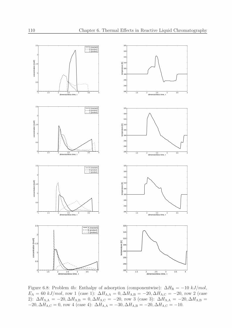
110 Chapter 6. Thermal Effects in Reactive Liquid Chromatography
1 1.5 2 2.5 3 3.5 40
0.5
1
1.5
2
2.5
dimensionless time, τ
conc
entr
atio
n [m
ol/l]
A (reactant)B (product)C (product)
1 1.5 2 2.5 3 3.5 4285
290
295
300
305
310
315
320
325
dimensionless time, τ
tem
pera
ture
[K]
1 1.5 2 2.5 3 3.5 40
0.5
1
1.5
2
2.5
dimensionless time, τ
conc
entr
atio
n [m
ol/l]
A (reactant)B (product)C (product)
1 1.5 2 2.5 3 3.5 4285
290
295
300
305
310
315
320
325
dimensionless time, τ
tem
pera
ture
[K]
1 1.5 2 2.5 3 3.5 40
0.5
1
1.5
2
2.5
dimensionless time, τ
conc
entr
atio
n [m
ol/l]
A (reactant)B (product)C (product)
1 1.5 2 2.5 3 3.5 4285
290
295
300
305
310
315
320
325
dimensionless time, τ
tem
pera
ture
[K]
1 1.5 2 2.5 3 3.5 40
0.5
1
1.5
2
2.5
dimensionless time, τ
conc
entr
atio
n [m
ol/l]
A (reactant)B (product)C (product)
1 1.5 2 2.5 3 3.5 4285
290
295
300
305
310
315
320
dimensionless time, τ
tem
pera
ture
[K]
Figure 6.8: Problem 4b: Enthalpy of adsorption (componentwise): ∆HR = −10 kJ/mol,EA = 60 kJ/mol, row 1 (case 1): ∆HA,A = 0,∆HA,B = −20,∆HA,C = −20, row 2 (case2): ∆HA,A = −20,∆HA,B = 0,∆HA,C = −20, row 3 (case 3): ∆HA,A = −20,∆HA,B =−20,∆HA,C = 0, row 4 (case 4): ∆HA,A = −30,∆HA,B = −20,∆HA,C = −10.

6.4. Demonstrations of thermal effects 111
1 1.5 2 2.5 3 3.5 40
0.5
1
1.5
2
2.5
dimensionless time, τ
conc
entr
atio
n [m
ol/l]
A (reactant)B (product)C (product)
1 1.5 2 2.5 3 3.5 4285
290
295
300
305
310
315
320
325
dimensionless time, τ
tem
pera
ture
[K]
1 1.5 2 2.5 3 3.5 40
0.5
1
1.5
2
2.5
dimensionless time, τ
conc
entr
atio
n [m
ol/l]
A (reactant)B (product)C (product)
1 1.5 2 2.5 3 3.5 4285
290
295
300
305
310
315
320
325
dimensionless time, τ
tem
pera
ture
[K]
1 1.5 2 2.5 3 3.5 40
0.5
1
1.5
2
2.5
dimensionless time, τ
conc
entr
atio
n [m
ol/l]
A (reactant)B (product)C (product)
1 1.5 2 2.5 3 3.5 4285
290
295
300
305
310
315
320
325
dimensionless time, τ
tem
pera
ture
[K]
1 1.5 2 2.5 3 3.5 40
0.5
1
1.5
2
2.5
dimensionless time, τ
conc
entr
atio
n [m
ol/l]
A (reactant)B (product)C (product)
1 1.5 2 2.5 3 3.5 4285
290
295
300
305
310
315
320
325
dimensionless time, τ
tem
pera
ture
[K]
Figure 6.9: Problem 5: Influence of dispersion terms. ∆HA,i = −20 kJ/mol, i=A,B,C,∆HR = −10 kJ/mol, EA = 60 kJ/mol, row 1 (case 1): PeM = 104, P eE = 104 row 2(case 2): PeM = 200, P eE = 0 row 3 (case 3): PeM = 0, P eE = 200, row 4 (case 4):PeM = 200, P eE = 200.

112 Chapter 6. Thermal Effects in Reactive Liquid Chromatography
6.5 Conclusion
In this chapter, reactive liquid chromatography was investigated theoretically considering
thermal effects that originate from heats of reaction and adsorption enthalpies. The sys-
tematic parametric studies carried out demonstrate that the related temperature gradients
can significantly influence the achievable conversion and separation. A high resolution finite
volume method was applied to numerically solve the mass and energy balances describing
this non-isothermal process. The scheme is robust, gives high order accuracy on coarse
grids and resolves sharp discontinuities. In order to verify the numerical results, several
consistency tests related to the mass and energy conservations, and evaluations of trivial
studies are carried out. The results prove the accuracy of the numerical scheme and agree
well with theoretical predictions for limiting cases. The key parameters that influence the
reactor performance were systematically investigated. It was found that the heats of reac-
tion and the enthalpies are the reason for complex concentration and temperature profiles.
It is important to mention, that higher conversion can be achieved under non-isothermal
conditions as compared to isothermal chromatographic reactor operation. It was observed,
that in particular an exothermic heat of reaction can be source for the development of a
positive thermal waves leading to significant improvements in conversion and separation.
The simulation results acquired in this study emphasize the necessity to account in more
detail for thermal effects in reactive liquid chromatography. Further research is required,
to further optimize internal temperature profiles.

Chapter 7
Summary and Conclusions
In this thesis models developed to describe, non-reactive and reactive liquid chromato-
graphic processes under isothermal and non-isothermal conditions were theoretically stud-
ied. Both analytical and numerical investigations were the focus of this work. The equi-
librium dispersive model and the lumped kinetic model were analyzed using Dirichlet and
Robin boundary conditions. These models constitute of systems of convection-diffusion-
reaction partial differential equations with dominating convective terms that are coupled
with differential or algebraic equations.
For linear adsorption isotherms, the Laplace transformation was used to solve analytically
the special case of single-component movements in chromatographic columns. The Laplace
transformation technique has already been used to solve linear chromatographic models
[42, 43]. In this work, statistical moments up to the third order were derived and calculated
for both types of models and boundary conditions.
For nonlinear adsorption isotherms, numerical techniques are the only tool to obtain solu-
tions of the models. However, the strong nonlinearities of realistic thermodynamic func-
tions (isotherms) and the stiffness of reaction terms pose major difficulties for the numerical
schemes. For this reason, computational efficiency and accuracy of numerical methods are
of large relevance. They were a focus of this dissertation. The high resolution finite volume
scheme of Koren [39] and the discontinuous Galerkin finite element method were imple-
mented to solve isothermal non-reactive and reactive chromatographic models. The second
to third order accurate Koren scheme is a flux-limiting finite volume scheme in which fluxes
113

114 Chapter 7. Summary and Conclusions
are limited by using a nonlinear minmod limiter. This limiting procedure guarantees the
positivity of the scheme by suppressing numerical oscillations, usually encountered in the
numerical schemes of second and higher orders. The suggested DG-scheme satisfies the
TVB property and gives second order accuracy. The scheme can be easily extended to
higher orders by using high order basis functions and by employing better slope limiters,
for example reconstruction with the WENO limiters [69]. This method incorporates the
ideas of numerical fluxes and slope limiters in a very natural way to capture the physically
relevant discontinuities without producing spurious oscillations in their vicinity. In contrast
to the finite volume schemes, the DG-scheme is well suited to handle complicated geome-
tries and avoids the extension of mesh stencil that allows the incorporation of boundary
conditions uniformly.
Analytical solutions obtained in the Laplace domain were used to validate the numeri-
cal predictions generated by using proposed schemes. Analytical solutions were obtained
for the single component linear equilibrium dispersive and lumped kinetic models using
Dirichlet and Robin boundary conditions. Statistical moments of step responses were cal-
culated and compared with numerical predictions for both types of models and boundary
conditions. Good agreements up to the third moment were observed which assured the
accuracy of suggested numerical solution techniques. A close connection between equilib-
rium dispersive and lumped kinetic models was pointed out and the strength of the simpler
equilibrium dispersive model for linear isotherm was illustrated.
Available experimental results were also utilized to validate the numerical results. Due to
unavailability of exact nonlinear models solutions, the accuracy of the proposed schemes
were validated against some other flux-limiting finite volume schemes available in the liter-
ature. Both schemes were found to be robust, give a high order accuracy on coarse grids,
and resolve sharp discontinuities. The numerical test problems showed that the suggested
DG-scheme produced slightly more resolved solutions than the high resolution scheme of
Koren, especially at sharp discontinuities. However, desirable results can also be achieved
by using the Koren scheme. On the basis of these results, one can conclude that both DG
and Koren schemes are highly recommendable methods for the numerical approximation

115
of linear and nonlinear chromatographic models. The suggested methods are efficient, ac-
curate, and suited to carry out simulations of dynamic of chromatographic processes in
packed columns.
Another important focus of this dissertation was to analyze thermal effects on reactive
liquid chromatographic process that originate from reaction and adsorption enthalpies.
Through systematic parametric studies, it was shown that temperature gradients can sig-
nificantly influence the achievable conversion and separation. A high resolution finite vol-
ume method was implemented to numerically approximate the coupled mass and energy
balances describing the non-isothermal process. In order to verify the numerical results,
several consistency tests related to mass and energy conservations, and evaluations of triv-
ial studies were carried out. The results proved the accuracy of applied numerical scheme,
the correctness of the model formulation and agreed well with theoretical predictions for
limiting cases. The key parameters that influence the reactor performance were systemati-
cally investigated. It was found that the heats of reaction and the adsorption enthalpies are
the reason for complex concentration and temperature profiles. It is important to mention,
that higher conversion can be achieved in certain cases under non-isothermal conditions
as compared to isothermal chromatographic reactor operation. The simulation results ac-
quired in this study emphasize the necessity to account in more detail for thermal effects
in reactive liquid chromatography. Further work is required, to optimize the reactor by
controlling internal temperature profiles.
The present contribution was based on the numerical approximation of chromatographic
processes occuring in a single column. However, the suggested numerical schemes can
also be used to deal with the non-linearity of more complicated processes, such as multi-
column moving-bed processes and periodic operations. Especially, to develop an efficient
and accurate numerical scheme for the simulated moving bed chromatography process will
be the main focus of our future research work. Being a continuous purification process,
simulated moving bed chromatography has higher outputs and requires less solvent than
conventional batch chromatography.
In this dissertation, the equilibrium dispersive and lumped kinetic models were studied.

116 Chapter 7. Summary and Conclusions
Future research tasks include the extension of our work to more complicated models, such as
the general rate model. The simulation of such more detailed models are quite complicated.
Therefore, further work is required to investigate the model and to search for efficient
and accurate numerical schemes. In addition, the operating conditions for preparative
chromatography, as for any industrial process, must be optimized. Such optimization is
based on thorough understanding of process variables and economics. We will optimize
the non-isothermal process to improve yield, productivity and, ultimately, to reduce the
operational cost. Optimization of this complex process is a challenging task due to the
nonlinearity of chromatographic models and the large number of operating variables. It is
therefore, necessary to use effective mathematical tools as developed in this work to solve
the nonlinear problems.
Finally, it can be concluded that accurate numerical tools are essential to understand and
illustrate complex front propagation phenomena taking place in chromatographic columns.

Appendix A
Mathematical Derivations
Here, we present the complete derivations of the first three moments for both equilibrium
dispersive and lumped kinetic models with Dirichlet and Danckwerts boundary conditions.
Equilibrium dispersive model with Dirichlet boundary conditions
In this part, the moments of equilibrium dispersive model with Dirichlet boundary condi-
tions are derived. By taking x = 1 and c0 = 1, the Eq. (4.13) can be written as
C(x = 1, s) =1
sexp
(
Pe
2−
1
2
√
Pe2 + 4PeL
u(1 + aF )s
)
. (A.1)
With
Pe =Lu
Dapp. (A.2)
We further define
b1 = Pe(1 + aF )L
u. (A.3)
The moment generating property of the Laplace transform is used exploiting (e.g. [99])
µn = (−1)n lims→0
dn(sC)
dsn, n = 0, 1, 2, 3, · · · (A.4)
Thus, the zeroth moment is given as
µ0 = lims→0
sC(x = 1, s) = lims→0
exp
(Pe
2−
1
2
√
Pe2 + 4b1s
)
= 1. (A.5)
The first initial moment can be obtained from Eq. (A.4) as
µ1 = (−1) lims→0
d(sC)
ds= lim
s→0
exp(
Pe2− 1
2
√
Pe2 + 4b1s)
√
Pe2 + 4b1s. (A.6)
117

118 Chapter A. Mathematical Derivations
Thus,
µ1 =b1Pe
=L
u(1 + aF ). (A.7)
The second initial moment can be derived from the relation given in Eq. (A.4) as
µ2 = (−1)2 lims→0
d2(sC)
ds2, (A.8)
where
d2(sC)
ds2=
2b12 exp
(Pe2− 1
2
√
Pe2 + 4b1s)
(Pe2 + 4a1s
)3/2+
b21 exp(
Pe2− 1
2
√
Pe2 + 4b1s)
Pe2 + 4a1s. (A.9)
Thus, the second initial moment is given as
µ2 =b1
2(2 + Pe)
Pe3=
2L
u3Dapp(1 + aF )2 +
L2
u2(1 + aF )2. (A.10)
The second central moment or the variance is given by the following expression
µ′
2 = µ2 − µ12 =
b12
Pe3=
2L
u3Dapp(1 + aF )2. (A.11)
Finally, the third initial moment is again obtained using Eq. (A.4)
µ3 = (−1)3 lims→0
d3(sC)
ds3=
b13
Pe5(6Pe+ 12 + Pe2), (A.12)
or
µ3 =L3
u3(1 + aF )3
(6Dapp
Lu+
12D2app
L2u2+ 1
)
. (A.13)
The third central moment can be calculated from the moments given above using the
subsequent formula
µ′
3 = µ3 − 3µ1µ2 + 2µ13 . (A.14)
Thus
µ′
3 =12LD2
app
u5(1 + aF )3. (A.15)

119
Equilibrium dispersive model with Danckwerts boundary conditions
Here, the moments of the equilibrium dispersive model with Danckwerts boundary condi-
tions are presented.
The zeroth moment is given as
µ0 = lims→0
A exp(λ1x) +B exp(λ2x) = 1. (A.16)
The first initial moment is obtained as
µ1 =b1Pe
=L
u(1 + aF ). (A.17)
The second initial moment is calculated as
µ2 =2b1
2
Pe4
(
−1 + Pe+Pe2
2+ e−Pe
)
, (A.18)
or
µ2 =2D2
app(1 + Fa)2
u4
(
−1 +Lu
Dapp+
L2u2
2D2app
+ e−Lu/Dapp
)
. (A.19)
The second central moment is given as
µ′
2 =2b1
2e−Pe
Pe4(−ePe + ePePe+ 1
)
=2L
u3Dapp(1 + aF )2
(
1 +Dapp
Lu
(e−Lu/Dapp − 1
))
. (A.20)
Lastly, the third initial moment is provided as
µ3 =b1
3
Pe6(−24 + 6Pe+ 6Pe2 + Pe3 + 24e−Pe + 18e−PePe
). (A.21)
The third central moment formula based on (A.14) is given below
µ′
3 =12LD2
app(1 + aF )3
u5
[(
1 +2Dapp
Lu
)
e−Lu/Dapp +
(
1−2Dapp
Lu
)]
. (A.22)
Lumped kinetic model with Dirichlet boundary conditions:
This part presents the moments for the lumped kinetic model with Dirichlet boundary
conditions. For x = 1 and c0 = 1, Eq. (4.25) can be rewritten as
C(x = 1, s) =1
sexp
(
b
2−
1
2
√
b2 + 4a1s−4a2
s+ a3+ 4a4
)
. (A.23)

120 Chapter A. Mathematical Derivations
With
b = Pe =Lu
D, a1 = Pe
L
u, a2 =
L2
ǫD
k2a
(1− ǫ), a3 =
k
(1− ǫ), a4 =
L2ak
ǫD. (A.24)
The zeroth moment is given as
µ0 = lims→0
exp
(
b
2−
1
2
√
b2 + 4a1s−4a2
s+ a3+ 4a4
)
= 1. (A.25)
The first initial moment is calculated as
µ1 = lims→0
4(
a1 +a2
(s+a3)2
)
exp(
b2− 1
2
√
b2 + 4a1s−4a2s+a3
+ 4a4
)
4√
b2 + 4a1s−4a2s+a3
+ 4a4, (A.26)
or
µ1 =a1a3
2 + a2a32b
=L
u(1 + aF ). (A.27)
The second initial moment is again derived using Eq. (A.8) with
d2(sC)
ds2=
4(
a1 +a2
(s+a3)2
)
exp(
b2− 1
2
√
b2 + 4a1s−4a2s+a3
+ 4a4
)
8(
b2 + 4a1s−4a2s+a3
+ 4a4
)3/2
+2 a2 exp
(b2− 1
2
√
b2 + 4a1s− 4 a2s+a3
+ 4a4
)
(
b2 + 4a1s−4a2s+a3
+ 4a4
)1/2
(s+ a3)3
+4(
a1 +a2
(s+a3)2
)
exp(
b2− 1
2
√
b2 + 4a1s−4a2s+a3
+ 4a4
)
16(
b2 + 4a1s−4a2s+a3
+ 4a4
) . (A.28)
Then
µ2 =1
a34b3(2a1
2a34 + 4a1a3
2a2 + 2a22 + 2a2a3b
2 + ba12a3
4 + 2ba1a32a2 + ba2
2), (A.29)
or
µ2 =2LD(1 + aF )2
u3+
1
k
(2LaF (1− ǫ)
u
)
+L2
u2(1 + aF )2. (A.30)
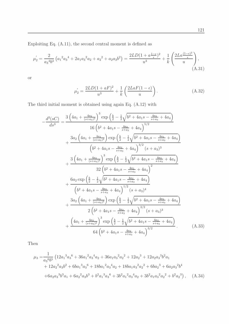
121
Exploiting Eq. (A.11), the second central moment is defined as
µ′
2 =2
a34b3(a1
2a34 + 2a1a3
2a2 + a22 + a2a3b
2)=
2LD(1 + a1−ǫǫ)2
u3+
1
k
(
2La (1−ǫ)2
ǫ
u
)
,
(A.31)
or
µ′
2 =2LD(1 + aF )2
u3+
1
k
(2LaF (1− ǫ)
u
)
. (A.32)
The third initial moment is obtained using again Eq. (A.12) with
−d3(sC)
ds3=
3(
4a1 +4a2
(s+a3)2
)3
exp(
b2− 1
2
√
b2 + 4a1s−4a2s+a3
+ 4a4
)
16(
b2 + 4a1s−4a2s+a3
+ 4a4
)5/2
+3a2
(
4a1 +4a2
(s+a3)2
)
exp(
b2− 1
2
√
b2 + 4a1s−4a2s+a3
+ 4a4
)
(
b2 + 4a1s−4a2s+a3
+ 4a4
)3/2
(s+ a3)3
+3(
4a1 +4a2
(s+a3)2
)3
exp(
b2− 1
2
√
b2 + 4a1s−4a2s+a3
+ 4a4
)
32(
b2 + 4a1s−4a2s+a3
+ 4a4
)2
+6a2 exp
(b2− 1
2
√
b2 + 4a1s−4a2s+a3
+ 4a4
)
(
b2 + 4a1s−4a2s+a3
+ 4a4
)1/2
(s+ a3)4
+3a2
(
4a1 +4a2
(s+a3)2
)
exp(
b2− 1
2
√
b2 + 4a1s−4a2s+a3
+ 4a4
)
2(
b2 + 4a1s−4a2s+a3
+ 4a4
)3/2
(s+ a3)3
+
(
4a1 +4a2
(s+a3)2
)3
exp(
b2− 1
2
√
b2 + 4a1s−4a2s+a3
+ 4a4
)
64(
b2 + 4a1s−4a2s+a3
+ 4a4
)3/2. (A.33)
Then
µ3 =1
a36b5(12a1
3a36 + 36a1
2a34a2 + 36a1a3
2a22 + 12a2
3 + 12a2a33b2a1
+ 12a22a3b
2 + 6ba13a3
6 + 18ba12a3
4a2 + 18ba1a32a2
2 + 6ba23 + 6a2a3
2b4
+6a2a33b3a1 + 6a2
2a3b3 + b2a1
3a36 + 3b2a1
2a34a2 + 3b2a1a3
2a22 + b2a2
3), (A.34)

122 Chapter A. Mathematical Derivations
or
µ3 =L3
u3(1 + aF )3
(6D
Lu+
12D2
L2u2+ 1
)
+6L2(1 + aF )a(1− ǫ)
u3k
(2D
L+
(1− ǫ)u2
Lk(1 + aF )+ u
)
.
(A.35)
Using (A.14), the third central moment is given as
µ′
3 =12LD2
u5(1 + aF )3 +
6L2(1 + aF )aF (1− ǫ)
ku3
(2D
L+
(1− ǫ)u2
Lk(1 + aF )
)
. (A.36)
or
µ′
3 =12LD2
u5(1 + aF )3 +
1
k
(12LD(1 + aF )aF (1− ǫ)
u3
)
+1
k2
(6LaF (1− ǫ)2
u
)
. (A.37)
Lumped kinetic model with Danckwerts boundary conditions
This part discusses the derivation of moments for lumped kinetic model with Danckwerts
boundary conditions.
The zeroth moment is again given as
µ0 = 1. (A.38)
The first initial moment corresponding again to Eq. (A.7)
µ1 =a1a3
2 + a2a32b
=L
u(1 + aF ). (A.39)
The second initial moment is given as
µ2 =e−b
a34b4(4a1a3
2a2 − 2eba12a3
4 + 2ebba22 + ebb2a2
2
− 4eba1a32a2 + 2ebba1
2a34 + ebb2a1
2a34 + 2a2e
ba3b3 + 4ebba1a3
2a2
+2ebb2a12a3
2a2 + 2a12a3
4 + 2a22 − 2beba2
2). (A.40)
The second central moment is defined as, c.f. (A.11),
µ′
2 =2L
u3D(1 + aF )2
(
1 +D
Lu
(e−Lu/D − 1
))
+1
k
(2LaFǫ
u
)
. (A.41)

123
The third initial moment is given as
µ3 =e−b
a36b6(24a1
3a36 + 24a2
3 + 72a12a3
4a2 + 72a1a32a2
2 + 12a22a3b
2 + 18ba13a3
6
+54ba12a3
4a2 + 54ba1a32a2
2 + 6a2eba3
2b5 + 6a13a3
6ebb2 − 12a22eba3b
2 + 12a22eba3b
3
+6ebba13a3
6 + 6a22a3b
4 + ebb3a13a3
6 + 18ba23 + 6ebba2
3 + ebb3a23 − 24eba1
3a36
+6ebb2a23 − 24eba2
3 + 18ebba12a3
4a2 − 12a2eba3
3b2a1 + 12a2eba3
3b3a1 + 18ebba1a32a2
2
+6eba2a33b4a1 + 3ebb3a1
2a34a2 + 3ebb3a1a3
2a22 + 18a1
2a34ebb2a2 + 18a1a3
2ebb2a22
−72eba12a3
4a2 − 72eba1a32a2
2 + 12a2a33b2a1
). (A.42)
The third central moment is using again (A.14) as
µ′
3 =12LD2(1 + aF )3
u5
[(
1 +2D
Lu
)
e−Lu/D +
(
1−2D
Lu
)]
+1
k
[12DLaF 2ǫ(1 + aF )
u3
(D
Lue−Lu/D + 1−
D
Lu
)]
+1
k2
(6LaF 3ǫ2
u
)
. (A.43)

Appendix B
Nomenclatureai Henry constants of component i, [-]b nonlinearity parameter in Eq. (2.18), [l/mol]ci liquid phase concentration of component i, [mol/l]cp concentration in the pores of particles i, [mol/l]Cp heat capacity, [kJ/gK]d column diameter, [m]Dapp apparent dispersion coefficient in EDM [m2/s]D dispersion coefficient in LKM [m2/s]EA activation energy, [kJ/mol]EH a relative percentage error in energy balance, [-]Eξ a relative percentage error in molar concentration ξ, [-]F phase ratio, [-]∆HA enthalpy of adsorption, [kJ/mol]∆HR enthalpy of reaction, [kJ/mol]∆Hout temperature at the column outlet, [kJ ]Ij jth mesh interval, [-]k mass transfer coefficient, [1/s]kfor forward reaction rate constant, [1/s]Keq reaction equilibrium constant, [-]K∗
eq reaction equilibrium constant, [mol/l]L column length, [m]ni molar amount of component i, [mol]Nc number of components, [-]Nt number of theoretical plates, [-]N number of grid cells, [-]Pl Legendre polynomial of order l (−)PeM Peclet number of mass balance, [-]PeE Peclet number of energy balance, [-]q∗i solid phase concentration of component i, [mol/l]r rate of chemical reaction, [mol/ls]R gas constant, 8.314×10⁻³, [kJ/molK]t time, [s]
124

125
Nomenclature (continued)
T pure thermal waveu interstitial velocity, [m/s]V volume, [l]
V volumetric flow rate, [l/s]XA conversion of reactant A, [-]z spatial coordinate, [m]Greek symbols
νi stoichiometric coefficient of component iλ conductivity coefficient, [m2kJ/slK]η very small number∆xj width of mesh interval Ij∆t time stepǫ external porosityξ extent of reaction, [mol]x dimensionless distance, x = z
L
τ dimensionless time, τ = tuL
ρ density, [g/l]φl local basis function of order lµn n-th initial normalized momentµ
′
n n-th central momentSuperscripts
in inlet valueinit initial valueout outlet profileL liquid phasep∗ p* is order of numerical schemeS solid phaseSubscripts
E energyi i is the number of Nc componentsj j is the number of discretized cellsm m is the number of Nc + 1 pseudo-componentsM massAbbreviations
BCs boundary conditionsDG discontinuous GalerkinEDM equilibrium dispersive modelFBCR fixed-bed chromatographic reactorFDMs finite difference methodsFEMs finite element methodsFVMs finite volume methodsLKM lumped kinetic modelODEs ordinary differential equationsPDEs partial differential equationsTVB total variation boundedness

Bibliography
[1] Aizinger, V., Dawson, C., Cockburn, B., Castillo, P., 2000. Local discontinuous
Galerkin method for contaminant transport. Advances in Water Resources 24, 73-87.
[2] Bahhar, A., Baranger, J., Sandri, D., 1998. Galerkin discontinuous approximation of
the transport equation and viscoelastic fluid flow on quadrilaterals. Numerical Meth-
ods of Partial Differential Equations 14, 97-114.
[3] Bassi, F., Rebay, S., 1997. A high-order accurate discontinuous finite element method
for the numerical solution of the compressible Navier-Stokes equations. Journal of
Computational Physics 131, 267-279.
[4] Borren, T., Fricke, J.: Schmidt-Traub, H., (Ed.), 2005. Chromatographic reactors in
preparative chromatography of fine chemicals and pharmaceutical agents, Wiley-VCH
Verlag, Weinheim, 371-395.
[5] Broughton, D.B., 1961. Continuous sorption process employing fixed bed of sorbent
and moving inlets and outlet. US Patent 2, 985, 589.
[6] Carey, G.F., Finlayson, B.A., 1975. Orthogonal collocation on finite elements. Chem-
ical Engineering Science 30, 587-596.
[7] Chen, Z., Cockburn, B., Jerome, J., Shu, C.-W., 1995. Mixed-RKDG finite element
methods for the 2-D hydrodynamic model for semiconductor device simulation. VLSI
Design 3, 145-158.
126

BIBLIOGRAPHY 127
[8] Clough, R.W., 1960. The finite element method in plane stress analysis. Proceedings
of 2nd ASCE conference on Electronic computation, Pittsburgh, PA, September 8-9.
[9] Cockburn, B., Shu, C.-W., 1989. TVB Runge-Kutta local projection discontinuous
Galerkin finite element method for conservation laws II: General framework. Mathe-
matices of computation 52, 411-435.
[10] Cockburn, B., Lin, S.-Y., 1989. TVB Runge-Kutta local projection discontinuous
Galerkin finite element method for conservation laws III: One-dimensional systems.
Journal of Computational Physics 84, 90-113.
[11] Cockburn, B., Hou, S., Shu, C.-W., 1990. TVB Runge-Kutta local projection discon-
tinuous Galerkin finite element method for conservation laws IV: The multidimensional
case. Mathematices of computation 54, 545-581.
[12] Cockburn, B., Shu, C.-W., 1989. The Runge-Kutta discontinuous Galerkin finite ele-
ment method for conservation laws V: Multidimensional systems. Journal of Compu-
tational Physics 141, 199-224.
[13] Cockburn, B., Shu., C.-W., 2001. Runge Kutta discontinuous Galerkin methods for
convection-dominated problems. Journal of Scientific Computing 16, 173-261.
[14] Cockburn, B., Dawson, C., 2002. Approximation of the velocity by coupling discon-
tinuous Galerkin and mixed finite element methods for flow problems. Computational
Geosciences 6, 502-522.
[15] Craig, L.C., 1944. Identification of Small Amounts of Organic Compounds by Dis-
tribution Studies. II. Separation By Counter-current Distribution. Journal of Biology
Chemistry 155, 519-534.
[16] Cruz, P., Santos, J.C., Magalhas, F.D., Mendes, A., 2005. Simulation of separation
processes using finite volume method. Computer & Chemical Engineering Journal 30,
83-98.

128 BIBLIOGRAPHY
[17] Danckwerts, P.V., 1953. Continuous flow systems. Chemical Engineering Science 2,
1-9.
[18] Dinwinddie, J.A., Morgan, W.A., 1961. U.S. Patent 2, 976, 132, to Esso Research and
Engineering Company.
[19] Dondi, F., Remelli, M., 1986. The characteristic function-method in the stochastic-
theory of chromatography. Journal of Physical Chemistry 90, 1885-1891.
[20] Dreyer, W., Qamar, S., 2005. Second order accurate explicit finite volume schemes
for the solution of Boltzmann-Peierls equation. Journal of Applied Mathematics and
Mechnaics 85, 4-22.
[21] Eigenberger, G., Kolios, G., NieKen, U., 2007. Efficient reheating of a reverse-flow
reformer-An experimental study. Chemical Engineering Science 62, 4825-4841.
[22] Felinger, A., Cavazzini, A., Dondi, F., 2004. Equivalence of the microscopic and macro-
scopic models of chromatography: stochastic-dispersive versus lumped kinetic model.
Journal of Chromatography A 1043, 149-157.
[23] Frenz, J., Horvath, C.S., and Horvath (Ed.), 1988. High-performance liquid chro-
matography Advances and Perspectives, vol. 5. Academic Press, New York.
[24] Fricke, J., Schmidt-Traub, H., Kawase, M., 2005. Chromatographic reactor, Ullmann’s
Encyclopedia of Industrial Chemistry, Wiley-VCH Verlag, Weinheim.
[25] Ganetsos, G., Barker, P.E., 1993. Preparative and production scale chromatography,
vol. 61. Marcel Dekker, Inc., New York, 375-523.
[26] Gaziev, G.A., Roginskii, S.Z., Yanovskii, M.J., 1962. U.S.S.R. Patent 149, 398.
[27] Glockler, B., Dieter, H., Eigenberger, G., NieKen, U., 2006. Efficient reheating of a
reverse-flow reformer-An experimental study. Chemical Engineering Science 62, 5638-
5643.

BIBLIOGRAPHY 129
[28] Guiochon, G., 2002. Preparative liquid chromatography. Journal of Chromatography
A 965, 129-161.
[29] Guiochon, G., Lin, B., 2003. Modeling for preparative chromatography, Academic
Press, Amsterdam.
[30] Guiochon, G., Felinger, A., Shirazi, D.G., Katti, A.M., 2006. Fundamentals of prepar-
ative and nonlinear chromatography, 2nd ed., Academic Press imprint of Elsevier,
Boston.
[31] Holik, M., 2009. Application of discontinuous Galerkin method for the simulation of
3D inviscid compressible flows. Proceedings of ALGORITMY 304-312.
[32] Hughes, T.J.R., Brooks, A.N., 1979. A multidimensional upwind scheme with no cross-
wind diffusion. In Hughes, T.J.R., (Ed.), Finite Element Methods for Convection
Dominated Flows, ASME, New York, 19-35.
[33] Hughes, T.J.R., 1995. Multiscale phenomena: Green’s functions, the Dirichlet-to-
Neumann formulation, subgrid scale models, bubbles and the origins of stabilized
methods. Computer Methods in Applied Mechanics and Engineering 127, 387-401.
[34] Javeed, S., Qamar, S., Seidel-Morgenstern, A., Warnecke, G., 2011. Efficient and
accurate numerical simulation of nonlinear chromatographic processes. Computer &
Chemical Engineering 35, 2294-2305.
[35] Javeed, S., Qamar, S., Seidel-Morgenstern, A., Warnecke, G., 2011. A discontinuous
Galerkin method to solve chromatographic models. Journal of Chromatography A
1218, 7137-7146.
[36] Javeed, S., Qamar, S., Seidel-Morgenstern, A., Warnecke, G., 2012. Parametric study
of thermal effects in reactive liquid chromatography. Chemical Engineering Journal
191, 426-440.

130 BIBLIOGRAPHY
[37] Javeed, S., Qamar, S., Seidel-Morgenstern, A., Warnecke, G., 2013. Analysis and
numerical investigation of two dynamic models for liquid chromatography. Chemical
Engineering Science 90, 17-31.
[38] Jeansonne, M.S., Foley, J.P., 1992. Improved equations for the calculation of chro-
matographic figures of merit for ideal and skewed chromatographic peaks. Journal of
Chromatography A 594, 1-8.
[39] Koren, B. 1993. A robust upwind discretization method for advection, diffusion
and source terms. In Vreugdenhil, C.B., Koren, B., (Eds.), Numerical Methods for
Advection-Diffusion Problems, Volume 45 of Notes on Numerical Fluid Mechanics,
Braunschweig: Vieweg Verlag, 117-138.
[40] Kruglov, A., 1994. Methanol synthesis in a simulated countercurrent moving-bed ad-
sorptive catalytic reactor. Chemical Engineering Science 49, 4699-4716.
[41] Kubin, M., 1965. Beitrag zur Theorie der Chromatographie. Collection of Czechoslovak
Chemical Communications 30, 1104-1118.
[42] Kubin, M., 1965. Beitrag zur Theorie der Chromatographie. 11. Einfluss der Diffusion
Ausserhalb und der Adsorption Innerhalb des Sorbens- Korns. Collection of Czechoslo-
vak Chemical Communications 30, 2900-2907.
[43] Kucera, E., 1965. Contribution to the theory of chromatography: Linear non-
equilibrium elution chromatography. Journal of Chromatography A 19, 237-248.
[44] Kuhn, R., Winterstein, A., Lederer, E., 1931. The xaothophylls, Zeitschrift fur Phys-
iologische Chemie 197, 141-160.
[45] Kumar, A., Jaiswal, D.K., Kumar, N., 2009. Analytical solutions of one-dimensional
advection-diffusion equation with variable coefficients in a finite domain. Journal of
Earth System Science 118, 539-549.

BIBLIOGRAPHY 131
[46] Kurganov, A., Tadmor, E., 2000. New High-Resolution Central Schemes for Nonlinear
Conservation Laws and Convection-Diffusion Equations. Journal of Computational
Physics 160, 241-282.
[47] Langer, S.H., Patton, J.E., 1974. Chemical reactor applications of the gas chromato-
graphic column. In Purnell, H., (Ed.), New developments in gas chromatography,
Wiley, New York, 293-373.
[48] Lapidus, L., Amundson, N.R., 1952. Mathematics of adsorption in beds, VI. The effect
of longitudinal diffision in ion exchange and chromatographic columns. The Journal
of Physical Chemistry 56, 984-988.
[49] LeVeque, R.J., 1992. Numerical methods for conservation laws. Birkhauser Verlag,
Bassel, Germany.
[50] LeVeque, R.J., 2003. Finite Volume Methods for Hyperbolic Systems. Cambridge Uni-
versity Press, Cambridge.
[51] Lieres, E.V., Andersson, J., 2010. A fast and accurate solver for the general rate model
of column liquid chromatography. Computer & chemical Engineering 34, 1180-1191.
[52] Lim, Y.I., Jorgen, S.B., 2004. A fast and accurate numerical method for solving simu-
lated moving bed (SMB) chromatographic separation problems. Chemical Engineering
Science 59, 1931- 1947.
[53] Lim, Y.I., Jorgen, S.B., 2009. Performance evaluation of the conservation element and
solution element method in the SMB process simulation. Chemical Engineering and
Processing: Process Intensification 59, 1931- 1947.
[54] Ma, Z., Guiochon, G., 1991. Application of Orthogonal Collocation on Finite Elements
in the Simulation of Non-Linear Chromatography. Computer & chemical Engineering
15, 415-426.
[55] Magee, E.M., 1961. Canadian Patent 631, 882.

132 BIBLIOGRAPHY
[56] Mai, P., Tien, V.D., Mai, K.X., Seidel-Morgenstern, A., 2004. Analysis of heteroge-
neously catalyzed ester hydrolysis performed in a chromatographic reactor and in a
reaction calorimeter. Industrial & Engineering Chemistry Research 43, 4691-4702.
[57] Martin, A.J.P., Synge, R.L.M., 1941. A new form of chromatogram employing two
liquid phases: A theory of chromatography. 2. Application to the micro-determination
of the higher monoamino-acids in proteins. Biochemical Journal 35, 1358-1368.
[58] Mazzotti, M., 2009. Nonclassical composition fronts in nonlinear chromatography:
Delta-shock. Industrial & Engineering Chemistry Research 48, 7733-7752.
[59] Mazzotti, M., Tarafderb, A., Cornela, J., Gritti, F., Guiochon, G., 2010. Experimental
evidence of a delta-shock in nonlinear chromatography. Journal of Chromatography A
1217, 2002-2012.
[60] Medi, B., and Amanullah, M., 2011. Application of a Finite-Volume Method in the
Simulation of Chromatographic Systems: Effects of Flux Limiters. Industrial & Engi-
neering Chemistry Research 50, 1739-1748.
[61] Minceva, M., Pais, L., Rodrigues, A., 2003. Cyclic steady state of simulated mov-
ing bed processes for enantiomers separation. Chemical Engineering and Processing:
Process Intensification 42, 93-104.
[62] Miyabe, K., Guiochon, G., 2000. Influence of the modification conditions of alkyl
bonded ligands on the characteristics of reversed-phase liquid chromatography. Journal
of Chromatography A 903, 1-12.
[63] Miyabe, K., Guiochon, G., 2003. Measurement of the parameters of the mass transfer
kinetics in high performance liquid chromatography. Journal of Separation Science 26,
155-173.
[64] Miyabe, K., 2007. Surface diffusion in reversed-phase liquid chromatography using
silica gel stationary phases of different C1 and C18 ligand densities. Journal of Chro-
matography A 1167, 161-170.

BIBLIOGRAPHY 133
[65] Miyabe, K., 2009. Moment analysis of chromatographic behavior in reversed-phase
liquid chromatography. Journal of Separation Science 32, 757-770.
[66] Qamar, S., Warnecke, G., 2005. A high order kinetic flux-spitting method for the
special relativistic magnetohydrodynamics. Journal of Computational Physics 205,
182-204.
[67] Qamar, S., Warnecke, G., 2006. A space-time conservative method for hyperbolic sys-
tems with stiff and non stiff source terms. Communications in Computational Physics
1, 451-480.
[68] Qamar, S., 2008. Modeling and simulation of population balances for particulate pro-
cesses, Habilitation thesis, Faculty of Mathematics, OVGU, Magdeburg, Germany.
[69] Qiu, J.X., Shu, C.-W., 2004. Hermite WENO schemes and their application as limiters
for Runge-Kutta discontinuous Galerkin method: One dimensional case. Journal of
Computational Physics 193, 115-135.
[70] Qiu, J.X., Khoo, B.C., Shu, C.-W., 2006. A numerical study for the performance of
the Runge-Kutta discontinuous Galerkin method based on different numerical fluxes.
Journal of Computational Physics 212, 540-565.
[71] Reed, W.H., Hill, T.R., 1973. Triangular mesh methods for the neutron transport
equation. Los Alamos Scientific Laboratory Report LA-UR, 73-79.
[72] Rhee, H.-K., Aris, R., Amundson, N.R., 1989. First-order partial differential equations.
Theory and Application of Hyperbolic Systems of Quasilinear Equations, Volume. II.
Prentice-Hall, New Jersey.
[73] Rice, R.G., Do, D.D., 1995. Applied Mathematics and Modeling for Chemical Engi-
neers, New York, Wiley.
[74] Roe, P.L., 1986. Characteristic-based schemes for the Euler equations. Annual Review
of Fluid Mechanics 18, 337-365.

134 BIBLIOGRAPHY
[75] Rouchon, P., Schoenauer, M., Valentin, P., Vidal-Madjar, C., Guiochon, G., 1985.
Theory of propagation of finite concentration bands in gas chromatography. A numer-
ical solution of the ideal problem. Journal of Physical Chemistry 89, 2076-2082.
[76] Ruthven, D. M., 1984. Principles of adsorption and adsorption processes. Wiley-
Interscience.
[77] Sainio, T., 2005. Ion-exchange resins as stationary phase in reactive chromatography.
Acta Universitatis Lappeenrantaensis 218, PhD thesis, Lappeenranta University of
Technology, 2005.
[78] Sainio, T., Kaspereit, M., Kienle, A., Seidel-Morgenstern, A., 2007. Thermal effects
in reactive liquid chromatography. Chemical Engineering Science 62, 5674-5681.
[79] Sainio, T., Zhang, L., Seidel-Morgenstern, A., 2011. Adiabatic operation of chromato-
graphic fixed-bed reactors. Chemical Engineering Journal 168, 861-871.
[80] Sardin, M., Schweich, D., Villermaux J., 1993. Preparative fixed-bed chromatographic
reactor. In Ganetsos, G., Barker, P.E., (Eds.), Preparative and Production Scale Chro-
matography, Marcel Dekker Inc., New York, USA, 477-522.
[81] Schmidt-Traub, H., Schulte, M., Seidel-Morgenstern, A., 2012. Preparative Chro-
matography, Weinheim, Germany: Wiley.
[82] Schneider, P. and Smith, J. M., 1968. Adsorption rate constants from chromatography.
A.I.Ch.E. Journal 14, 762-771.
[83] Seidel-Morgenstern, A., 1991. Analysis of boundary conditions in the axial dispersion
model by application of numerical Laplace inversion. Chemical Engineering Science
46, 2567-2571.
[84] Shipilova, O., Sainio, T., Haario H., 2008. Particle transport method for simulation
of multicomponent chromatography problems. Journal of Chromatography A 1204,
62-71.

BIBLIOGRAPHY 135
[85] Sundmacher, K., Kienle, A., Seidel-Morgenstern, A., 2005. Integrated Chemical Pro-
cesses, Weinheim, Germany, Wiley.
[86] Suzuki, M., Smith, J.M., 1971. Kinetic studies by chromatography. Chemical Engi-
neering Scienece 26, 221-235.
[87] Suzuki, M., 1973. Notes on Determining the Moments of the Impulse Response of the
Basic Transformed Equations. Journal of Chemical Engineering of Japan 6, 540-543.
[88] Sweby, P.K., 1984. High resolution schemes using flux limiters for hyperbolic conser-
vation laws. SIAM Journal on Numerical Analysis 30, 995-1011.
[89] Thiele, A., Falk, T., Tobiska, L., Seidel-Morgenstern, A., 2001. Prediction of elution
profiles in annular chromatography. Journal of Computer & Chemical Engineering 13,
1089-1101.
[90] Tien, V.D., Seidel-Morgenstern, A., 2011. Quantifying Temperature and Flow Rate
Effects on the Performance of a Fixed-bed Chromatographic Reactor. Journal of Chro-
matography A 1218, 8097-8109.
[91] Tien, V.D., Seidel-Morgenstern, A., Gruner, S., Kienle, A., 2005. Analysis of ester
hydrolysis reactions in a chromatographic reactor using equilibrium theory and a rate
model. Industrial & Engineering Chemistry Research 44, 9565-9574.
[92] Tien, V.D., 2007. Analysis of heterogeneously catalyzed ester hydrolysis reactions
in a fixed-bed Chromatographic reactor. PhD thesis, Faculty of Process and System
Engineering, OVGU, Magdeburg, Germany.
[93] Tiselius, A., 1943. Displacement development in adsorption analysis, Arkiv foer Kemi,
Mineralogi och Geologi 16A 194, 1-18.
[94] Toro, E.F., 1999. Riemann solvers and numerical method for fluid dynamics, Second
Edition, Springer-Verlag.

136 BIBLIOGRAPHY
[95] Toumi, A., Engell, S., Diehl, M., Bock, H.G., Schloder, J., 2007. Efficient optimization
of simulated moving bed processes. Chemical Engineering and Processing 46, 1067-
1084.
[96] Tswett, M., 1906. Physikalisch-chemische Studienuber das Chlorophyll. Die Adsorp-
tionen. Berichte der Deutschen Botanischen Gesellschaft 24, 316-323.
[97] Tswett, M., 1906. Adsorptionsanalyse und chromatographische Methode. Anwendung
auf die Chemie des Chlorophylls. Berichte der Deutschen Botanischen Gesellschaft 24,
384-393.
[98] Van Deemter, J.J., Zuiderweg, F.J., A. Klinkenberg, A., 1956. Longitudinal diffusion
and resistance to mass transfer as causes of nonideality in chromatography. Chemical
Engineering Science 5, 271-289.
[99] Van der Laan, Th., 1958. Letter to the Editors on Notes on the diffusion type model
for the longitudinal mixing in flow. Chemical Engineering Science 7, 187-191.
[100] Van Leer, B., 1977. Towards the ultimate conservative difference scheme, IV: a new
approach to numerical convection. Journal of Computational Physics 12, 276-299.
[101] Van Leer, B., Enguist, B.E., Osher, S., Somerville, R.C.J., 1985. Upwind-difference
methods for aerodynamic problems governed by the Euler equations, large-scale com-
putations in fluid mechanics. AMS series, American Mathematical Society, 327-336.
[102] Villermaux J., Rodrigues, A.E., Tondeur, D., (Eds.), 1981. The chromatographic re-
actor in precolation processes: Theory and applications, Sijthoffen Noordhoff, Alpena
an den Rijn, The Netherlands, 539-588.
[103] Webley, P.A., He, J., 2000. Fast solution-adaptive finite volume method for PSA/VSA
cycle simulation; 1 single step simulation. Computer & chemical Engineering 23, 1701-
1712.

BIBLIOGRAPHY 137
[104] Xiu, G., Li, P., Rodrigues, A.E., 2002. Sorption-enhanced reaction process with re-
active regeneration. Chemical Engineering Science 57, 3893-3908.
[105] Yongsunthon, I., Alpay, E., 1999. Design of periodic adsorptive reactors for the op-
timal integration of reaction, Separation and Heat Exchange. Chemical Engineering
Science 54, 2647-2657.
[106] Zechmeister, L., Cholnoky, L.V., 1937. Die chromatographische Adsorptionsmethode.
Grundlagen, Methodik, Anwendungen, Julius Springer, Wein.
[107] Zhang, P., Liu, R.-X., 2005. Hyperbolic conservation laws with space-dependent
fluxes: II. General study of numerical fluxes. Journal of Computational and Applied
Mathematics 176, 105-129.
[108] Zhang, X., Shu, C.-W., 2011. Positivity-preserving high order discontinuous Galerkin
schemes for compressible Euler equations with source terms. Journal of Computational
Physics 230, 1238-1248.
[109] Zienkiewicz, O.C., Chung, O.C., 1967. The finite element method in continumm and
structural mechanics, Mcgraw Hill.

Curriculum VitaePersonal Information
Name Shumaila JaveedDate of Birth 29.01.1985Place of Birth Rawalpindi, PakistanNationality PakistaniMarital Status Single
Education and Employment
2010-2013 PhD studies at the Otto-von-Guericke-Universty and the Max Planck Institutefor Dynamics of Complex Technical Systems, Magdeburg, Germany
2008-2010 MS(Mathematics), COMSATS Institute of Information Technology,Islamabad, Pakistan
2002-2006 BS(Mathematics), COMSATS Institute of Information Technology,Islamabad, Pakistan
2000-2002 F.Sc or Intermediate studies, Rawalpindi, Pakistan
1990-2000 Schooling, Rawalpindi, Pakistan
2007-2010 Lecturer, COMSATS Institute of Information Technology,Islamabad, Pakistan
Academic Honors
• Three months research scholarship from Max Planck Institute, Magdeburg, Germany
• Research productivity award from COMSATS, Islamabad, Pakistan
• Scholarship for BS(Mathematics) studies
• Acquired distinction at Matriculation and Intermediate level
138