Sensors 2015, 15, 9681-9702; doi:10.3390/s150509681

sensors ISSN 1424-8220

www.mdpi.com/journal/sensors

Article

Analysis and Experimental Kinematics of a Skid-Steering Wheeled Robot Based on a Laser Scanner Sensor

Tianmiao Wang, Yao Wu *, Jianhong Liang, Chenhao Han, Jiao Chen and Qiteng Zhao

Robotics Institute, Beihang University, Beijing 100191, China; E-Mails: wtm_itm@263.net (T.W.);

dommy_leung@263.net (J.L.); shasmyan@sina.cn (C.H.); chenjiao_1989@yeah.net (J.C.);

zqt_buaa@126.com (Q.Z.)

* Author to whom correspondence should be addressed; E-Mail: wuyao@me.buaa.edu.cn;

Tel./Fax: +86-10-8233-8271.

Academic Editor: Vittorio M.N. Passaro

Received: 11 February 2015 / Accepted: 17 April 2015 / Published: 24 April 2015

Abstract: Skid-steering mobile robots are widely used because of their simple mechanism

and robustness. However, due to the complex wheel-ground interactions and the kinematic

constraints, it is a challenge to understand the kinematics and dynamics of such a robotic

platform. In this paper, we develop an analysis and experimental kinematic scheme for a

skid-steering wheeled vehicle based-on a laser scanner sensor. The kinematics model is

established based on the boundedness of the instantaneous centers of rotation (ICR) of

treads on the 2D motion plane. The kinematic parameters (the ICR coefficient , the path

curvature variable and robot speed ), including the effect of vehicle dynamics, are

introduced to describe the kinematics model. Then, an exact but costly dynamic model is

used and the simulation of this model’s stationary response for the vehicle shows a

qualitative relationship for the specified parameters and . Moreover, the parameters of

the kinematic model are determined based-on a laser scanner localization experimental

analysis method with a skid-steering robotic platform, Pioneer P3-AT. The relationship

between the ICR coefficient and two physical factors is studied, i.e., the radius of the

path curvature and the robot speed . An empirical function-based relationship between

the ICR coefficient of the robot and the path parameters is derived. To validate the

obtained results, it is empirically demonstrated that the proposed kinematics model

significantly improves the dead-reckoning performance of this skid–steering robot.

OPEN ACCESS

Sensors 2015, 15 9682

Keywords: mobile robot; laser scanner; skid-steering; instantaneous centers of rotation;

experimental kinematics; dynamic model

1. Introduction

Skid-steering motion is widely used for wheeled and tracked mobile robots [1]. Steering in this way

is based on controlling the relative velocities of the left and right side drives. The robot turning

requires slippage of the wheels for wheeled vehicles. Due to their identical steering mechanisms,

wheeled and tracked skid-steering vehicles share many properties [2,3].

Like differential steering, skid steering leads to high maneuverability [4,5], and has a simple and

robust mechanical structure, leaving more room in the vehicle for the mission equipment [3,6]. In

addition, it has good mobility on a variety of terrains, which makes it suitable for all-terrain missions.

However, this locomotion scheme makes it difficult to develop kinematic and dynamic models that

can accurately describe the motion. It is very difficult for the skid-steering kinematics to predict the

exact motion of the vehicle only from its control inputs. As a result, the kinematics models with pure

rolling and no-slip assumptions for non-holonomic wheeled vehicles cannot apply in this case [2].

Furthermore, other disadvantages are that the motion tends to be energy inefficient, difficult to control,

and for wheeled vehicles, the tires tend to wear out faster [6,7].

Some previous studies have discussed the dynamic control of skid-steering mobile robots. A

dynamic model was presented for a skid-steering four-wheel robot and a non-holonomic constraint

between the robot’s lateral velocity and yaw rate was considered in [5]. A perfect wheel-ground

interaction was assumed. A simple Coulomb friction model was used to capture the wheel-ground

interaction and a nonlinear feedback controller was designed to track the desired path [6]. Yu and

Ylaya Chuy developed a skid-steering mobile robot dynamic model for general 2D motion and linear

3D motion [8,9]. This model was based on the functional relationship of shear stress to shear

displacement, which is different from the previous Coulomb-friction-based model [5,6]. It needs a lot

of computational effort to calculate a complex dynamics model in real-time, for example, this work

requires a number of integral operations, so the dynamic models for skid-steering may result too costly

for real-time motion control and dead-reckoning.

In the meantime, Maalouf et al. [10] and Kozlowski [11] separately considered the kinematics for

the relation between drive velocities and vehicle velocities without concerning themselves with major

skid effects. As we know, wheel slip plays a critical role in the kinematic and dynamic modeling of

skid-steering mobile robots. The slip information provides a connection between the wheel rotation

velocity and the linear motion of the robot platform. With an extended Kalman filter, the slip

estimation was performed from actual inertial readings and a kinematics model of the vehicle relates

the slip parameters to the track velocities [12]. Furthermore, an experimental method was developed to

determine the slip ratios. The slip coefficients of tracks were modeled as an exponential function of

path radius [13].

An extra trailer was designed to study the kinematic relationship for simultaneous localization and

mapping (SLAM) applications. It was concluded that an ideal differential-driven kinematics model for

Sensors 2015, 15 9683

wheeled robot cannot be used for skid-steering robots [14,15]. Meanwhile, geometric analogy with an

ideal differential-driven wheeled mobile robot was studied [2,7]. Experimental validations have been

conducted for both tracked vehicles and skid-steering mobile robots. These correspond to the position

of ideal differential drive wheels for a particular terrain. This is based on the fact that tread ICR values

are dynamics-dependent, but they lie within a bounded area at moderate speeds. A group of constant

kinematic parameters were derived as optimized values for the tread ICR on the plane. Specifically, we

find that tread ICR values vary with the speed of the robot and the path curvature, so it is necessary to

further describe the relationship between tread ICR values and curvature of the path and the

vehicle speed.

Building upon the research by Mandow [2] and Moosavian [13], we develop an experimental

kinematics model for a skid-steering mobile robot. The kinematics model based on ICR of both treads

on the motion plane is used [2], and we consider that tread ICR values change with the speed of the

robot and the path curvature by explicitly considering slip ratio [13]. A dynamic model based on the

research by Yu [8,9] and Wong [16,17] is developed for a simulation in order to estimate a potential

kinematics relationship. Because a laser scanner is accurate and efficient for mobile robot localization

and dead-reckoning [18,19], with a laser-scanner-based experimental method, an approximating

function is derived to describe the relationship between the ICR values of the robot and the radius of

curvature of the path and speed of the robot.

The main contribution in this paper is that the new analysis and experimental kinematic scheme of

the skid-steering robot reveal the underlying kinematic relationship between the ICR coefficient of the

robot and the path parameters. The simulation based on a dynamic model analysis shows a qualitative

relationship among the parameters theoretically specified before the experiment. An empirical function

relationship between the ICR values of the robot and the path parameters is derived with this

laser-scanner-based experimental method. Dead-reckoning performance shows that the empirical

function kinematics model improves the motion estimation accuracy significantly. This

laser-scanner-based method is easy to operate and does not add extra sensors or change the vehicle

mechanical structure and control system. The proposed model and analysis approach can be further

used for robot control, as an exact kinematics control can be used for a skid-steering robot [13].

The remainder of this paper is organized as follows: Section 2 presents the kinematic and dynamic

modeling of a four-wheel skid-steering mobile robot. A dynamic model based simulation to explain the

potential kinematics relationship is proposed. In Section 3 the laser-scanner-based localization method

is presented and the experiment results and analyses are given.

2. Model Analysis and Simulation

2.1. Kinematical Analogy of Skid-Steering with Differential Drive

Figure 1 shows the kinematics schematic of a skid-steering robot. We consider the following

model assumptions:

(1) the mass center of the robot is located at the geometric center of the body frame;

(2) the two wheels of each side rotate at the same speed;

Sensors 2015, 15 9684

(3) the robot is running on a firm ground surface, and four wheels are always in contact with the

ground surface.

Figure 1. The kinematics schematic of skid-steering mobile robot.

We define an inertial frame (X, Y) (global frame) and a local (robot body) frame (x, y), as shown in

Figure 1. Suppose that the robot moves on a plane with a linear velocity expressed in the local frame as = ( , , 0) and rotates with an angular velocity vector = (0,0, ) . If = ( , , ) is the

state vector describing generalized coordinate of the robot (i.e., the COM position, X and Y, and the

orientation of the local coordinate frame with respect to the inertial frame), then = , , denotes the vector of generalized velocities. It is straightforward to calculate the

relationship of the robot velocities in both frames as follows [6]:

= − 000 0 1 (1)

Let , i = 1,2,3,4 denote the wheel angular velocities for front-left, rear-left, front-right and

rear-right wheels, respectively. From assumption (2), we have: = = , = = (2)

Then the direct kinematics on the plane can be stated as follows: = (3)

where = ( , ) is the vehicle’s translational velocity with respect to its local frame, and is its

angular velocity, is the radius of the wheel.

When the mobile robot moves, we denote instantaneous centers of rotation (ICR) of the left-side

tread, right-side tread, and the robot body as , and , respectively. It is known that ,

Sensors 2015, 15 9685

and lie on a line parallel to the x-axis [7,16]. We define the x-y coordinates for ,

and as( , ) , ( , ) , and ( , ), respectively.

Note that treads have the same angular velocity as the robot body. We can get the

geometrical relation: = (4)= − (5)= − (6)= = = − (7)

From Equations (4)–(7), the kinematics relation (3) can be represented as: = (8)

Where the elements of matrix J depend on the tread ICR coordinates: = 1− − −−1 1 (9)

If the mobile robot is symmetrical, we can get a symmetrical kinematics model (i.e., the ICRs lie

symmetrically on the x-axis and = 0), so matrix can be written as the following form: = 12 0 0−1 1 (10)

where = = − is the instantaneous tread ICR value. Noted that = , = , for the

symmetrical model, the following equations can be obtained: = +2 = +2= 0= − +2 = − +2 (11)

Noted = 0, so that = . We can get the instantaneous radius of the path curvature: = = = +− + (12)

A non-dimensional path curvature variable λ is introduced as the ratio of sum and difference of

left- and right-side’s wheel linear velocities [1], namely: = +− + (13)

and we can rewrite Equation (12) as:

Sensors 2015, 15 9686

= +− + = (14)

We use a similar index as in Mandow’s work [2,7], then an ICR coefficient χ can be defined as: = − = 2 , ≥ 1 (15)

where denotes the lateral wheel bases, as illustrated in Figure 1. The ICR coefficient is equal to 1

when no slippage occurs (ideal differential drive). Note that the locomotion system introduces a

non-holonomic restriction in the motion plane because the non-square matrix has no inverse.

It is noted that the above expressions also present the kinematics for ideal wheeled differential drive

vehicles, as illustrated in Figure 2. Therefore, for instantaneous motion, kinematic equivalences can be

considered between skid-steering and ideal wheel vehicles. The difference between both traction

schemes is that whereas the ICR values for single ideal wheels are constant and coincident with the

ground contact points, tread ICR values are dynamics-dependent and always lie outside of the tread

centerlines because of slippage, so we can know that less slippage results in that tread ICRs are closer

to the vehicle.

Figure 2. Geometric equivalence between the wheeled skid-steering robot and the ideal

differential drive robot.

The major consequence of the study above is that the effect of vehicle dynamics is introduced in the

kinematics model. Although the model does not consider the direct forces, it provides an accurate

model of the underlying dynamics using lump parameters: and . Furthermore, from

assumptions (1) and (3), we get a symmetrical kinematics model, and an ICR coefficient χ from

Equation (15) is defined to describe the model. The relationship between ICR coefficient and the

vehicle motion path and velocity will be studied.

Sensors 2015, 15 9687

2.2. Dynamic Model for Kinematics Parameters Relationship

2.2.1. Skid-Steering Mobile Robot Dynamic Model

In Section 2.1, the effect of vehicle dynamics is introduced in the kinematics model. This section

develops dynamic models of a skid-steering wheeled vehicle for the cases of 2D motion. Using the

dynamic models, the relationship between the ICR coefficients and the path and velocity of the vehicle

motion will be studied in a simulation.

In contrast to dynamic models described in terms of the velocity vector of the vehicle [4], the

dynamic models here are described in terms of the angular velocity vector of the wheels. This is

because the wheel velocities are actually commanded by the control system, so this model form is

particularly beneficial for motion simulation.

Figure 3. Forces and moments acting on a wheeled skid-steering vehicle during a steady

state turn.

As in Figure 3, following Wong’s model [16], the dynamic model is given by: + + + − − = 0+ + + =− = 0 (16)

where is the vehicle velocity, and is the angle between the vehicle velocity and x-axis on the local frame. , , , are the longitudinal (friction) forces and , , , are the lateral

forces. , , , are external motion resistances on the four wheels. is the drive moment

and is the resistance moment.

Based on the wheel-ground interaction theory [16,17], the shear stress and shear displacement j

relationship can be described as:

Sensors 2015, 15 9688

= 1 − (17)

where is the normal pressure, is the coefficient of friction and is the shear deformation modulus.

Figure 4 depicts a skid-steering wheeled vehicle moving counterclockwise (CCW) at constant linear

velocity and angular velocity in a circle centered at from position (1) to position (2). The four

contact patches of the wheels with the ground are shadows in Figure 4. L and C are the patch-related distances. In the inertial X-Y frame, we define that , , , and , , , are respectively

the shear displacements and sliding velocity angle (opposite direction of sliding velocity). The readers

can refer to Yu’s work [9] for a detailed analysis. The longitudinal sliding friction and lateral force of

the four wheels can be expressed as follows: = (1 − ) +//

//= (1 − ) +/

//

/, (18)

= (1 − ) ( + )//

//= (1 − ) ( + )/

//

/, (19)

= (1 − ) +//

//= (1 − ) +/

//

/, (20)

= (1 − ) ( + )//

//= (1 − ) ( + )/

//

/, (21)

where , and are respectively the normal pressure, coefficient of friction, and shear deformation

modulus of the left wheels, and , and are the ones of the right wheels, respectively. With the

other parameters directly measured or given, such as mass of vehicle, m, patch-related distances, L and

C, width of wheel, b, and can be determined by /2( − ) when a uniform normal pressure

distributions assumption used ( = ). We share some parameters: , , and as in Yu’s

research [9], because the same platform (Pioneer P3-AT robot) and similar lab surface are used for

the simulation.

Sensors 2015, 15 9689

Y

XO

y

x

xl

y l

xr

y r

CG

v fr_y

vfr_x

vfr

γf

r

(xfr, yfr)

Ffr

y

x

C L

B

bx l

yl

x r

yrCG

R

(1)

(2)

(xrr, yrr)

(xrl, yrl)

(xfl, yfl)

ϕ

Figure 4. Motion of the skid-steering mobile robot wheel element on the lab surface

(firm ground) from position (1) to (2).

In Equation (16), the rolling resistance is denoted as . We can obtain the resistance force,

such that: = (22)

2.2.2. Dynamic Simulation

This section describes the dynamic simulation that has been used to get the relationship between the

treads’ ICRs and path. This model has been simulated for computing the treads’ ICR positions for the

Pioneer P3-AT robot. We set all of the key parameters for the model as listed in Table 1.

Table 1. The parameters for Pioneer P3-AT robot and terrain dynamic model.

Key Parameters Symbol Value

Mass of robot (kg) m 31 Width of robot (m) B 0.40 Length of robot (m) L 0.31

Length of C (m) C 0.24 Radius of tire (m) R 0.11

Width of wheel (m) b 0.05 Shear deformation modulus (m) , 0.00054 Coefficient of rolling resistance , 0.0371 Coefficient of friction, of 0.4437 Coefficient of friction, of 0.3093

Sensors 2015, 15 9690

The values of the ICR coefficient χ and nondimensional path curvature variable λ are computed by

solving the non-linear optimization problem with Equations (16)–(22):

, + (23)

where denotes the ith of N simulated data. When the skid-steering wheeled vehicle is in a constant

velocity circular motion, a set of different commanded turning radii is given by: = ( ), = 0, 1, 2 , … ,7 (24)

So we can use Equation (16) to get χ with respect to a special . The simulated results of χ vs. are

shown in Figure 5.

Figure 5. The dynamic simulated results of vs. with Pioneer P3-AT robot using

parameters in Table 1.

In Figure 5, we can find that decreases as increases, so there is a relationship between these two

parameters. In this simulation, we must note that these results are obtained by assuming that the

skid-steering mobile robot runs on the firm road and with special values of , , and .

Because these terrain parameters are difficult to determine, an exact relationship needs further

experimental identification.

3. Laser-Scanner-Based Experimental Kinematics Method

3.1. Proposed Algorithm

In this section, an easy-operating and effective experiment can be used to derive the symmetric

kinematics model and the ICR coefficient. When different angular speed control inputs and are

issued, we consider that the vehicle moves at a constant ICR value, then the following equation

can be applied: ( , ) = −2 (25)

where is the actual rotation angle. We can get by Equation (25). Then, we can use Equation (15)

to determine the ICR coefficient .

0 1 2 3 4 5 6 7 81.4

1.42

1.44

1.46

1.48

λ

χ

Simulation

Sensors 2015, 15 9691

A set of experiments have been performed. The robot is planned to follow eight different paths with

curvatures of radii: = ( ), = 0, 1, 2, … , 7 (26)

Note that is denoted in Equation (13). We can choose one of the experimental data as , and

on each path, five different speeds: = 0.1 ( / ), = 1, 2, … , 5 (27)

With Equations (26) and (27), we can get different ( , ) pairs. Therefore, 40 experiments will be

performed. The ICR coefficient is calculated in each experiment using Equations (15) and (25),

which requires measuring the actual speed of each side wheel during the experiment.

3.2. Laser-Scanner-Based Localization Method and Experiment Setup

The skid-steering mobile robot—a Pioneer P3-AT robot shown in Figure 6—is used for all testing

in this research [20], the parameters for the Pioneer P3-AT robot are listed in Table 1 in Section 2.2.2.

The P3-AT robot is driven by two motors on each side, and the two wheels of the same side are

connected by one chain, so the two wheels of each side rotate at the same speed.

In all of the experiments the field is faced with a tile. Final drive shaft speeds of the motors on the

robot are measured using two optical encoders. The optical encoders produce 2048 pulses per

resolution, and the interface chip provides quadrature encoding, producing a change of 8192 counts for

one revolution, or 0.0439° per count. A YL-100il wireless series port module, which can transmit data

transparently, is selected as wireless transmission part.

Figure 6. Skid-steering mobile robot platform—a Pioneer P3-AT mobile robot.

A laser scanner-based localization method is used for the position and heading measurements of the

robot. An overview of the proposed localization method and the robot control system are demonstrated

in Figure 7. In order to localize the robot a thin plate (indicated as (1) in Figure 7) is mounted on top of

the Pioneer P3-AT robot in the symmetric plane. A Sick LMS400-10000 laser scanner (3) is installed

at the same height, the data of which are used to localize the robot. We use a laptop to control the

Sensors 2015, 15 9692

Pioneer P3-AT robot (4) through a wireless serial port communication. The speed range of the robot is

about 0–0.6 m/s.

Figure 7. An overview of the proposed localization method based on a Laser Scanner.

(1) The thin plate; (2) Pioneer P3-AT robot; (3) Sick LMS400 Laser Scanner; (4) Laptop

software panel.

The Sick LMS400-1000 laser scanner [21], has a large dynamic measurement range of 0.7 m to 3 m

with 3 mm systematic error. The field of view of the laser scanner is 70° with 0.1° angular resolution

and 270 Hz–500 Hz scanning frequency. The measurement data from the laser scanner are sent to the

laptop using an Ethernet connection. The data of the LMS400 regarding the plate are extracted by a

clustering method. A line is fitted to the points. The line slope angle is equal to the heading angle, and

coordinates of its center are equal to the coordinates of robot geometric center. A median filter, an

edge filter and a mean filter are applied to the computed coordinates of robot to smooth the data as

much as possible. Measurements of position and heading from the plate can be updated at 135 Hz after

filtering. The calculations of position and heading from the plate are shown below.

Figure 8. Position and heading measurement from the plate based on LMS400-1000 Laser

Scanner for a real trajectory Ω of the robot’s center.

Sensors 2015, 15 9693

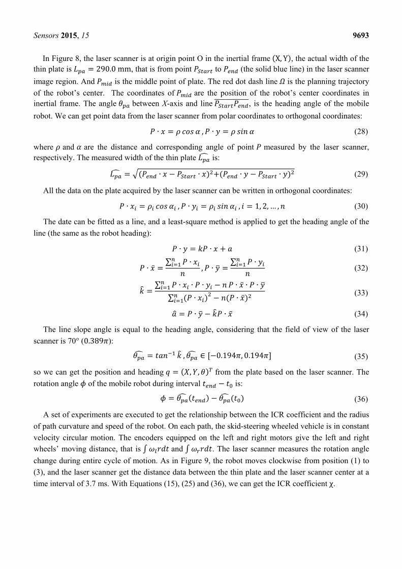
In Figure 8, the laser scanner is at origin point O in the inertial frame (X, Y), the actual width of the thin plate is = 290.0 mm, that is from point to (the solid blue line) in the laser scanner

image region. And is the middle point of plate. The red dot dash line is the planning trajectory

of the robot’s center. The coordinates of are the position of the robot’s center coordinates in inertial frame. The angle between X-axis and line , is the heading angle of the mobile

robot. We can get point data from the laser scanner from polar coordinates to orthogonal coordinates: ∙ = , ∙ = (28)

where and are the distance and corresponding angle of point measured by the laser scanner, respectively. The measured width of the thin plate is: = ( ∙ − ∙ ) +( ∙ − ∙ ) (29)

All the data on the plate acquired by the laser scanner can be written in orthogonal coordinates: ∙ = , ∙ = , = 1, 2, … , (30)

The date can be fitted as a line, and a least-square method is applied to get the heading angle of the

line (the same as the robot heading): ∙ = ∙ + (31)∙ = ∑ ∙ , ∙ = ∑ ∙ (32)

= ∑ ∙ ∙ ∙ − ∙ ∙ ∙∑ ( ∙ ) − ( ∙ ) (33)= ∙ − ∙ (34)

The line slope angle is equal to the heading angle, considering that the field of view of the laser

scanner is 70° (0.389 ): = , ∈ [−0.194 , 0.194 ] (35)

so we can get the position and heading = ( , , ) from the plate based on the laser scanner. The

rotation angle of the mobile robot during interval − is: = ( ) − ( ) (36)

A set of experiments are executed to get the relationship between the ICR coefficient and the radius

of path curvature and speed of the robot. On each path, the skid-steering wheeled vehicle is in constant

velocity circular motion. The encoders equipped on the left and right motors give the left and right wheels’ moving distance, that is and . The laser scanner measures the rotation angle

change during entire cycle of motion. As in Figure 9, the robot moves clockwise from position (1) to

(3), and the laser scanner get the distance data between the thin plate and the laser scanner center at a

time interval of 3.7 ms. With Equations (15), (25) and (36), we can get the ICR coefficient χ.

Sensors 2015, 15 9694

Figure 9. The laser scanner measurement during an entire cycle run from (1) start to

(3) end with the mobile robot.

3.3. Errors Analysis

The Sick laser scanner measurements errors are given by ∆ρ = 0.003 m and ∆α = . = 0.00174 rad [21], so the point data errors in orthogonal coordinates from

Equation (28) are: ∆ ∙ = |( ) |∆ + |( ) |∆ ≤ ∆ + | |∆ = 0.008 (37)

Similarly, ∆ ∙ = 0.008 m. When the robot moves, the maximum speed ≤ 0.7 m/s, and the

laser sample time ∆ = = . The dynamic error when the robot moves is: ∆ ∙ ≤ ; ∆ = 0.7 × 1135 = 0.005 m (38)

Note that ∆ . = ∆ ∙ , so the total point data measurement error is: ∆ ∙ = ∆ ∙ + ∆ ∙ = 0.013 m (39)

In Figure 8, with Equations (31), (33) and (36), denote ∈ − , and ∈ [1, 3], so the heading

angle is: = ( , ) = ( / ) , ∈ [0, 3√2], ∈ [ 1√2 , 3] (40)

and we have the heading angle error:

Sensors 2015, 15 9695

∆ = ∆ + ∆ = + ∆ + + ∆ ≤ √2∆ = 0.018 (41)

With Equation (25), we obtain: ( , ) = −2 = ( , , ) = −2 (42)

where and are the displacement distance measured by the left and right wheel encoders,

respectively, expressed in millimeters after correction. We note that the position errors are ∆ and ∆ , ∆ and ∆ are obtained by measuring the actual traveled distance d in straight motion, and the

results are ∆ = 0.00026 m, ∆ = 0.00020 m. Note that ∆ = 0.018 rad with Equation (41). Let ∆ denote the ICR value error for : ∆ = ∆ + ∆ + ∆ = 0.007 (43)

Note that is not less than 0.2 m with a width of robot = 0.40 m . The ICR value error ∆ = 0.007 m, corresponding to extremely small estimate error, is sufficient for further testing.

3.4. Results

Data are collected in real time and processed off line with MATLAB. Figure 10a shows a

comparison of the measured width of the plate from the laser scanner and the actual value. The

measured ones, shown as a dot line red line, lies close enough to the actual value (a solid blue line). In

Figure 10b, the mean difference between measured width and actual value is shown. In Table 2, it

shows that the mean value of measured width is 0.289 m and the standard deviation is 0.003 m, and the maximum error is − 0.01 m, corresponding to an extremely small ICR value

estimatation error. The results demonstrate the effectiveness and the feasibility of the proposed laser

scanner-based method.

(a) (b)

Figure 10. (a) A comparison of the measured width of the plate from the laser scanner and

the actual value; (b) Error between measured width and actual one.

0 0.5 1 1.5 2 2.5 3 3.5 4270

275

280

285

290

295

300

305

310

time(s)

Lpa

(m

m)

L

pa Measurement

Lpa

Actual

0 0.5 1 1.5 2 2.5 3 3.5 4-10

-8

-6

-4

-2

0

2

4

6

8

10

time(s)

Err

or

(mm

)

Sensors 2015, 15 9696

Table 2. Mean value and errors of measured width of the plate from the laser scanner.

Test Parameters (m) (m) Max. Error (m)

Width of the Plate ( ) 0.2890 0.003 −0.01

Figure 11 shows the position and heading and velocity of robots calculated by the laser

scanner-based localization algorithm during the experiment for speed of 0.25 m/s and curvature radius

of 0.475 m.

(a) (b)

Figure 11. Position and velocity of robots calculated by the proposed algorithm.

(a) position and heading; (b) velocity.

Figure 12 depicts that the ICR coefficient χ for various path curvatures and vehicle velocity. In

Table 3, the mean values μ and standard derivations σ of the ICR coefficient χ are shown. It shows that

the maximum relative error is less than 1%, and the maximum σ is no larger than 0.01, so the

differences between different χ with respect to corresponding λ can be distinguished, with this ICR

coefficient measurement accuracy. Furthermore we can find that Figure 12a represents the similar

trends as in Figure 5. By increasing the path curvature (increasing λ), the ICR coefficient χ decreases.

This implies a specific behavior for χ with respect to λ. Meanwhile, in Figure 12b, the ICR coefficient

remains almost constant with increasing velocity v, at certain λ.

(a) (b)

Figure 12. The calculated ICR coefficient χ for various: (a) path curvatures with = 0.1, 0.2, … 0.5 / ; and (b) robot speeds with = 0.1, 0.2, … 0.5 / with = 0, 1, 2, … , 7.

0 0.5 1 1.5 2 2.5 3 3.5 40

1

2

3

4

5

time(s)

posi

tion(

m o

r ra

d)

X(m)Y(m)θ(rad)

0 0.5 1 1.5 2 2.5 3 3.5 4-0.5

0

0.5

1

1.5

time(s)

velo

city

dX/dt(m/s)dY/dt(m/s)dθ/dt(rad/s)

0 2 4 6 8 101.4

1.42

1.44

1.46

1.48

λ

χ

υ=0.1m/s

υ=0.2m/s

υ=0.3m/s

υ=0.4m/s

υ=0.5m/s

0 100 200 300 400 500 6001.4

1.42

1.44

1.46

1.48

vehicle velocity(mm/s)

χ

λ =0

λ =1

λ =2

λ =3

λ =4

λ =5

λ =6

λ =7

Sensors 2015, 15 9697

Table 3. The calculated ICR coefficient for various .

Parameters Max. Relative Error

0 1.4662 0.0033 0.34% 1 1.4480 0.0065 0.59% 2 1.4394 0.0055 0.62% 3 1.4341 0.0068 0.71% 4 1.4215 0.0080 −0.92% 5 1.4232 0.0050 0.52% 6 1.4165 0.0077 0.77% 7 1.4115 0.0043 0.30%

In order to reveal the relationship, an approximate function is then used to define as a function of

the non-dimensional path curvature variable : ( ) = 1 + 1 + | | , ∈ [0, 10] (44)

where a and b are determined by a curve fit of the experimental data, > 0, > 0. We run 10 sets of

experiments with various on the lab surface. Numerical values of parameters = 0.4728, = 0.0538 are obtained using a nonlinear least-square algorithm for the function given in Equation (44),

and substituted as: ( ) = 1 + 0.47281 + 0.0538| | , ∈ [0, 10] (45)

Figure 13 shows versus using the approximating function and experimental data when = 0.3 m/s . The solutions obtained from the simulated and experimental methods are also

summarized in this figure. From a qualitative standpoint, experimental results are coherent with those

obtained in simulation. The simulation data are a little bigger than experimental results because of

uncertain model parameters, e.g., the coefficient of rolling resistance, coefficient of friction, and

shear modulus.

Figure 13. Experimental data curve, simulation data curve and data-fitted curve for with

respect to , when = 0.3 / .

0 1 2 3 4 5 6 7 81.4

1.42

1.44

1.46

1.48

λ

χ

Experimental data curveFitted data curveSimulation data curve

Sensors 2015, 15 9698

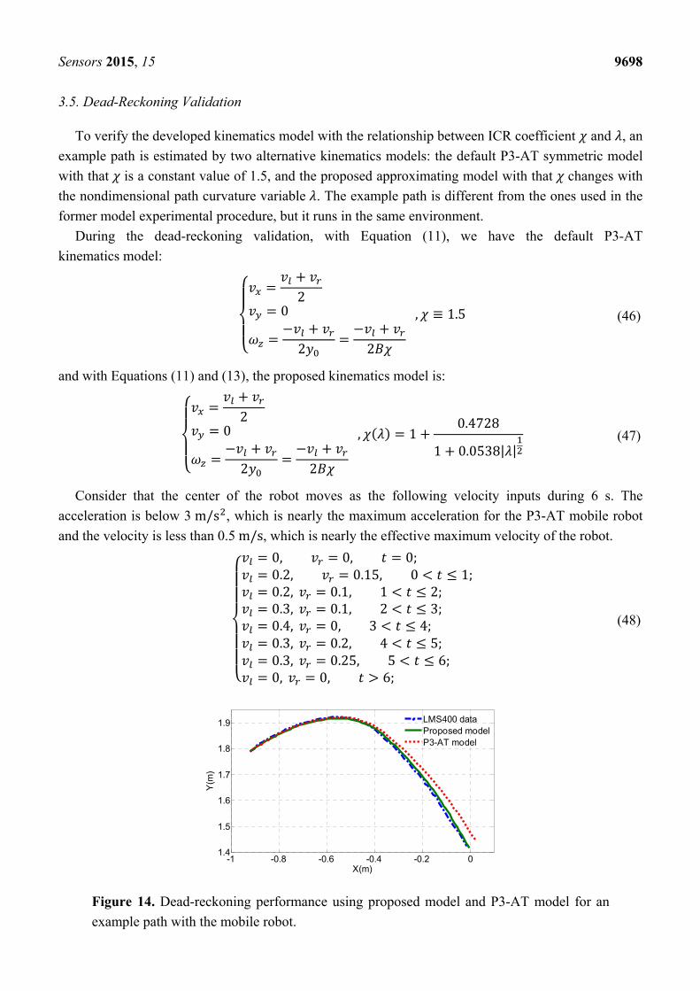
3.5. Dead-Reckoning Validation

To verify the developed kinematics model with the relationship between ICR coefficient and , an

example path is estimated by two alternative kinematics models: the default P3-AT symmetric model

with that is a constant value of 1.5, and the proposed approximating model with that changes with

the nondimensional path curvature variable . The example path is different from the ones used in the

former model experimental procedure, but it runs in the same environment.

During the dead-reckoning validation, with Equation (11), we have the default P3-AT

kinematics model: = +2= 0= − +2 = − +2 , ≡ 1.5 (46)

and with Equations (11) and (13), the proposed kinematics model is: = +2= 0= − +2 = − +2 , ( ) = 1 + 0.47281 + 0.0538| | (47)

Consider that the center of the robot moves as the following velocity inputs during 6 s. The

acceleration is below 3 m/s , which is nearly the maximum acceleration for the P3-AT mobile robot

and the velocity is less than 0.5 m/s, which is nearly the effective maximum velocity of the robot. = 0, = 0, = 0;= 0.2, = 0.15, 0 < ≤ 1;= 0.2, = 0.1, 1 < ≤ 2;= 0.3, = 0.1, 2 < ≤ 3;= 0.4, = 0, 3 < ≤ 4;= 0.3, = 0.2, 4 < ≤ 5;= 0.3, = 0.25, 5 < ≤ 6;= 0, = 0, > 6; (48)

Figure 14. Dead-reckoning performance using proposed model and P3-AT model for an

example path with the mobile robot.

-1 -0.8 -0.6 -0.4 -0.2 01.4

1.5

1.6

1.7

1.8

1.9

X(m)

Y(m

)

LMS400 dataProposed modelP3-AT model

Sensors 2015, 15 9699

Figure 14 shows the estimation of the path based on dead-reckoning (only drive shaft encoders are

used) according to the default P3-AT model and the proposed model, and the LMS400 laser scanner

data provide the actual position and heading. It can be seen that the proposal model achieves better

dead reckoning estimation accuracy than that of the default P3-AT model.

Cartesian error and its norm are depicted in Figure 15. The proposed model has a smaller position

error within 0.03 m, and a smaller angle error within 0.1 rad. Also, mean squared performance values

obtained in the validation path are show in Table 4.

(a)

(b)

Figure 15. Dead-reckoning errors using the proposed model and the P3-AT model for an

example path with the mobile robot. (a) Magnitude of position errors in X axis and Y axis;

(b) position magnitude errors and heading errors.

Table 4. Mean squared performance values of position and heading errors.

NO. ∆ (m) ∆ (m) ∆ (rad)

P3-AT model 0.0169 0.0101 0.0438 Proposed model 0.0273 0.0119 0.0778

Meanwhile, estimated ICR coefficient χ during the example path is presented in Figure 16. In fact,

the ICR coefficient χ varies as the path changes (it is not a constant value of 1.5).

1 2 3 4 5 6 7-0.05

0

0.05

time(s)

Mag

nitu

de o

f err

ors

in X

-axi

s

Proposed modelP3-AT model

1 2 3 4 5 6 7-0.02

0

0.02

0.04

time(s)

Mag

nitu

de o

f err

ors

in Y

-axi

s

Proposed modelP3-AT model

1 2 3 4 5 6 70

0.02

0.04

0.06

time(s)

Mag

nitu

de o

f er

rors

Proposed modelP3-AT model

1 2 3 4 5 6 7-0.2

0

0.2

time(s)

Hea

ding

err

ors

Proposed modelP3-AT model

Sensors 2015, 15 9700

Figure 16. ICR coefficient χ using the proposed model and the P3-AT model for an

example path with the mobile robot.

4. Conclusions/Outlook

We develop an analysis and experimental kinematics scheme of a skid-steering wheeled vehicle

based-on a laser scanner sensor. The ICR coefficient χ and a nondimensional path curvature variable λ

are introduced to describe the potential model relationship. The dynamic models based simulation

results show that there is some relationship between these two parameters. The laser-scanner-based

method experimentally derives the approximating function between and . The obtained function is

validated on a sample path. It was shown that the proposed kinematics model estimated for a

skid-steering mobile robot improves the system performance in terms of reduced dead-reckoning

errors, with a smaller position error within 0.03 m, and a smaller angle error within 0.1 rad with

respect to the default P3-AT model. This test method is easy to operate without adding extra sensors or

changing the vehicle mechanical structure and control system. The proposed model and analysis

approach can be further used for odometry or to map desired vehicle motion, such as vehicle speed and

angular rate, to required wheel speeds.

However, we use the assumptions 2 and 3, which the robot is running on a firm ground surface, and

four wheels with the same speed are always in contact with the ground surface. Some mobile robots

run on loose soil and in many 4/6 wheels drive (4/6WD) mobile robots, the wheels of each side rotate

at different speeds, raising the question of whether a similar result be obtained in a different

environment using this method? For future work, it would be interesting to validate the model on

different terrains. The current experimental testing results are obtained when acceleration a < 3 m s⁄

and velocity < 0.5 m s⁄ due to the limitations of the robotic platform. Thus, further experiments will

be implemented to discuss this problem at higher acceleration and velocity in the future.

Acknowledgments

This research is supported by the National High-Tech Research & Development Program of China

(Grant NO. 2011AA040202).

1 2 3 4 5 6 71.4

1.42

1.44

1.46

1.48

1.5

1.52

time(s)

χ

Proposed model with fitted curveP3-AT model

Sensors 2015, 15 9701

Author Contributions

All authors have significant contributions to this article. Tianmiao Wang and Yao Wu conceived

and designed the activity. Yao Wu, the corresponding author, was mainly responsible for the dynamics

model and kinematics model method with Jianhong Liang. Chenhao Han, was responsible for the

dynamics model and simulation for this model. Jiao Chen and Qiteng Zhao, performed the experiment

and data collection. Yao Wu and Chenhao Han wrote the paper.

Conflicts of Interest

The authors declare no conflict of interest.

References

1. Yi, J.; Wang, H.P.; Zhang, J.; Song, D. Kinematic modeling and analysis of skid-steered mobile

robots with applications to low-cost inertial-measurement-unit-based motion estimation.

IEEE Trans. Robot. 2009, 25, 1087–1097.

2. Mandow, A.; Martinez, J.L.; Morales, J.; Blanco, J.; García-Cerezo, A.J.; Gonzalez, J.

Experimental kinematics for wheeled skid-steer mobile robots. In Proceedings of

IEEE/RSJ International Conference on Intelligent Robots and Systems, San Diego, CA, USA,

29 October–2 November 2007; pp. 1222–1227.

3. Yi, J.; Zhang, J.; Song, D.; Jayasuriya, S. IMU-based localization and slip estimation for

skid-steered mobile robots. In Proceedings of IEEE/RSJ International Conference on Intelligent

Robots and Systems, San Diego, CA, USA, 29 October–2 November 2007; pp. 2845–2850.

4. Caracciolo, L.; Luca, A.D.; Iannitti, S. Trajectory tracking control of a four-wheel differentially

driven mobile robot. In Proceedings of IEEE/RSJ International Conference on Robotics and

Automation, Detroit, MI, USA, 10–15 May 1999; pp. 2632–2638.

5. Yi, J.; Song, D.; Zhang, J.; Goodwin, Z. Adaptive trajectory tracking control of skid-steered

mobile robots. In Proceedings of IEEE/RSJ International Conference on Robotics and

Automation, Rome, Italy, 10–14 April 2007; pp. 2605–2610.

6. Kozlowski, K.; Pazderski, D.; Modeling and control of a 4-wheel skid-steering mobile robot.

Int. J. Appl. Math. Comput. Sci. 2004, 14, 477–496.

7. Martinez, J.L.; Mandow, A.; Morales, J.; Pedraza, S.; García-Cerezo, A.J. Approximating

kinematics for tracked mobile robots. Int. J. Robot. Res. 2005, 24, 867–878.

8. Yu, W.; Chuy, O.; Collins, E.G.; Hollis, P. Dynamic Modeling of a Skid-Steered Wheeled

Vehicle with Experimental Verification. In Proceedings of IEEE/RSJ International Conference on

Intelligent Robots and Systems, St. Louis, MO, USA, 11–15 October 2009; pp. 4211–4219.

9. Yu, W.; Chuy, O.; Collins, E.G.; Hollis, P. Analysis and experimental verification for dynamic

modeling of a skid-steered wheeled vehicle. IEEE Trans. Robot. 2010, 26, 340–353.

10. Maalouf, E.; Saad, M.; Saliah, H. A higher level path tracking controller for a four-wheel

differentially steered mobile robot. Robot. Auton. Syst. 2006, 54, 23–33.

Sensors 2015, 15 9702

11. Kozlowski, K.; Pazderski, D. Practical stabilization of a skid-steering mobile robot—A

kinematic-based approach. In Proceedings of IEEE 3rd Conference on Mechatronics, Budapest,

Hungary, 3 July 2006; pp. 519–524.

12. Le, A.; Rye, D.; Durrant-Whyte, H. Estimation of track-soil interactions for autonomous tracked

vehicles. In Proceedings of IEEE/RSJ International Conference on Robotics and Automation,

Albuquerque, NM, USA, 10–14 April 1997; pp. 1388–1393.

13. Moosavian, S.A.A.; Kalantari, A. Experimental slip estimation for exact kinematics modeling and

control of a tracked Mobile Robot. In Proceedings of IEEE/RSJ International Conference on

Intelligent Robots and Systems, Nice, France, 22–26 September 2008; pp. 95–100.

14. Anousaki, G.; Kyriakopoulos, K. A dead-reckoning scheme for skid-steered vehicles in outdoor

environments. In Proceedings of IEEE/RSJ International Conference on Robotics and

Automation, New Orleans, LA, USA, 26 April–1 May 2004; pp. 580–585.

15. Anousaki, G.; Kyriakopoulos, K. Simultaneous localization and map building of skid-steered

robots. IEEE Robot. Autom. Mag. 2007, 14, 79–89.

16. Wong, J.; Chiang, C. A general theory for skid steering of tracked vehicles on firm ground. In

Proceedings of the Institution of Mechanical Engineers. Available online: http://pid.sagepub.com/

content/215/3/343.full.pdf (accessed on 23 April 2015).

17. Wong, J. Theory of Ground Vehicles, 3rd ed.; Wong, J.; John Wiley & Sons, Inc.: New York, NY,

USA, 2001; pp. 389–418.

18. Martinez, J.L.; Gonzalez, J.; Morales, J.; Mandow, A.; García-Cerezo, A.J. Mobile robot motion

estimation by 2D scan matching with genetic and iterative closest point algorithms. J. Field Robot.

2006, 23, 21–34.

19. Duan, Z.; Cai, Z.; Min, H. Robust Dead Reckoning System for Mobile Robots Based on Particle

Filter and Raw Range Scan. Sensors 2014, 14, 16532–16562.

20. Technical Description: Pioneer P3-AT Mobile Robot. Available online: http://www.mobilerobots.com

(accessed on 11 February 2015).

21. Technical Description: LMS400 Laser Measurement Sensor. Available online: http://www.sick.com

(accessed on 11 February 2015).

© 2015 by the authors; licensee MDPI, Basel, Switzerland. This article is an open access article

distributed under the terms and conditions of the Creative Commons Attribution license

(http://creativecommons.org/licenses/by/4.0/).