Embed Size (px)
Citation preview

Analysis and Design of Robust StabilizingModified Repetitive Control Systems
Zhongxiang Chen
GUNMA UNIVERSITY
March 2013


ABSTRACT
In control system practice, high precision tracking or attenuation for periodic signals
is an important issue. Repetitive control is known as an effective approach for such
control problems. The internal model principle shows that the repetitive control
system which contains a periodic generator in the closed-loop can achieve zero steady-
state error for reference input or completely attenuate disturbance. Due to its simple
structure and high control precision, repetitive control has been widely applied in
many systems. To improve existing results on repetitive control theory, this thesis
presents theoretical results in analysis and design repetitive control system. The main
work and innovations are listed as follows:
We propose a design method of robust stabilizing modified repetitive controllers
for multiple-input/multiple-output plants with uncertainties. The parameterization
of all robust stabilizing modified repetitive controllers for multiple-input/multiple-
output plant with uncertainty is obtained by employing H∞ control theory based on
the Riccati equation. The robust stabilizing controller contains free parameters that
are designed to achieve desirable control characteristic. In addition, the bandwidth
of low-pass filter has been analyzed. In order to simplify the design process and avoid
the wrong results obtained by graphical method, the robust stability conditions are
converted to LMIs-constraint conditions by employing the delay-dependent bounded
real lemma. When the free parameters of the parameterization of all robust stabiliz-
ing controllers is adequately chosen, then the controller works as robust stabilizing
modified repetitive controller.
For a time-varying periodic disturbances, we give an design method of an opti-
mal robust stabilizing modified repetitive controller for a strictly proper plant with
time-varying uncertainties. A modified repetitive controller with time-varying delay
structure, inserted by a low-pass filter and an adjustable parameter, is developed for
this class of system. Two linear matrix inequalities LMIs-based robust stability con-
ditions of the closed-loop system with time-varying state delay are derived for fixed

parameters. One is a delay-dependent robust stability condition that is derived based
on the free-weight matrix. The other robust stability condition is obtained based
on the H∞ control problem by introducing a linear unitary operator. To obtain the
desired controller, the design problems are converted to two LMI-constrained opti-
mization problems by reformulating the LMIs given in the robust stability conditions.
The validity of the proposed method is verified through a numerical example.

Contents
Chapter1 Introduction . . . . . . . . . . . . . . . . . . . . . . . . . . . 1
1.1 Background . . . . . . . . . . . . . . . . . . . . . . . . . . . 2
1.2 Repetitive control principle . . . . . . . . . . . . . . . . . . . 3
1.3 Modified repetitive controller . . . . . . . . . . . . . . . . . . 5
1.4 Review on modified repetitive control system design . . . . . 8
1.4.1 Frequency domain analysis-based design method . . . 9
1.4.2 Linear matrix inequality-based design method . . . . 10
1.4.3 H∞ robust design method . . . . . . . . . . . . . . . 11
1.4.4 Two-degree-of-freedom structure design method . . . 12
1.4.5 Two-dimensional-based design method . . . . . . . . 13
1.4.6 Parameterization design method . . . . . . . . . . . . 16
1.4.7 Existing problems . . . . . . . . . . . . . . . . . . . . 18
1.5 Organization of the thesis . . . . . . . . . . . . . . . . . . . 19
Chapter2 Robust Stabilizing Problem for Multiple-Input/Multiple-
Output Plants . . . . . . . . . . . . . . . . . . . . . . . . . . 23
2.1 Introduction . . . . . . . . . . . . . . . . . . . . . . . . . . . 23
2.2 Problem Formulation . . . . . . . . . . . . . . . . . . . . . . 26
2.3 The parameterization of all robust stabilizing modified repet-
itive controllers for MIMO plants . . . . . . . . . . . . . . . 28
2.4 Control characteristics . . . . . . . . . . . . . . . . . . . . . 34
2.5 Design parameters . . . . . . . . . . . . . . . . . . . . . . . . 37
2.5.1 Design parameters for control performance . . . . . . 37
i

2.5.2 Design parameters for robust stability conditions . . 39
2.5.3 Robust stability condition based on linear matrix in-
equalities (LMIs) . . . . . . . . . . . . . . . . . . . . 43
2.6 Numerical example . . . . . . . . . . . . . . . . . . . . . . . 46
2.7 Conclusions . . . . . . . . . . . . . . . . . . . . . . . . . . . 54
Chapter3 Robust Stabilizing Problem for Time-varying periodic Sig-
nals . . . . . . . . . . . . . . . . . . . . . . . . . . . . . . . . . 57
3.1 Introduction . . . . . . . . . . . . . . . . . . . . . . . . . . . 57
3.2 Problem statement and preliminaries . . . . . . . . . . . . . 60
3.3 Robust stability conditions . . . . . . . . . . . . . . . . . . . 65
3.4 Design procedure . . . . . . . . . . . . . . . . . . . . . . . . 76
3.5 Numerical example . . . . . . . . . . . . . . . . . . . . . . . 77
3.6 Conclusions . . . . . . . . . . . . . . . . . . . . . . . . . . . 80
Chapter4 Conclusions and Future Work . . . . . . . . . . . . . . . . . 81
4.1 Conclusions . . . . . . . . . . . . . . . . . . . . . . . . . . . 81
4.2 Future Work . . . . . . . . . . . . . . . . . . . . . . . . . . . 82
Bibliography . . . . . . . . . . . . . . . . . . . . . . . . . . . . . . . . . . 87
ii

List of Figures
1.1 Generator of periodic signals with period-time L[s] . . . . . . . . . . 4
1.2 Conventional repetitive control system . . . . . . . . . . . . . . . . . 4
1.3 Conventional modified repetitive control system . . . . . . . . . . . . 6
1.4 Bode plots of repetitive controller CR(s) (a) and modified repetitive
controller CRM(s) (b) . . . . . . . . . . . . . . . . . . . . . . . . . . 8
1.5 Two-degree-of-freedom modified repetitive control system . . . . . . . 12
2.1 Modified repetitive control system with uncertainty . . . . . . . . . . 26
2.2 Block diagram of H∞ control problem . . . . . . . . . . . . . . . . . . 29
2.3 Closed-loop system for Q(s) ∈ H∞ and ∥Q(s)∥∞ < 1 . . . . . . . . . 39
2.4 The nyquist plot of det(Qd1(s) +Qd2(s)e−sT ) . . . . . . . . . . . . . . 48
2.5 Largest singular value plot of Q(s) . . . . . . . . . . . . . . . . . . . 49
2.6 The nyquist plot of det(Qd1(s) +Qd2(s)e−sT ) when τd 1,2 = 0.001 . . 50
2.7 Largest singular value plot of Q(s) when τd 1,2 = 0.001 . . . . . . . . 50
2.8 Largest singular value plot of ∆(s) and gain plot of WT (s) . . . . . . 51
2.9 Response of the error e(t) for the reference input r(t) . . . . . . . . . 52
2.10 Response of the output y(t) for the disturbance d(t) . . . . . . . . . . 53
2.11 Response of the output y for the disturbance d(t) . . . . . . . . . . . 54
3.1 Flat cam grinding system . . . . . . . . . . . . . . . . . . . . . . . . 58
3.2 Rotation speed of servomotor . . . . . . . . . . . . . . . . . . . . . . 58
3.3 The new repetitive control system . . . . . . . . . . . . . . . . . . . . 62
3.4 The repetitive control system with uncertainties . . . . . . . . . . . . 63
3.5 Equivalent diagram of Figure 3.4 . . . . . . . . . . . . . . . . . . . . 71
iii

3.6 Disturbance signal used in simulations . . . . . . . . . . . . . . . . . 78
3.7 Time-varying period, τ(t) . . . . . . . . . . . . . . . . . . . . . . . . 78
3.8 Derivative of τ(t), τ(t) . . . . . . . . . . . . . . . . . . . . . . . . . . 78
3.9 Response of the output y(t) for the disturbance d(t) with our repetitive
controller . . . . . . . . . . . . . . . . . . . . . . . . . . . . . . . . . 79
3.10 Response of the output y(t) for the disturbance d(t) without our repet-
itive controller . . . . . . . . . . . . . . . . . . . . . . . . . . . . . . . 79
iv

1
Chapter 1
Introduction
People often completely master a new learned skill through repetition. By repeating
the same action, a person gradually comes to understand the essential points, and
achieves a significant efficiency and precision. This process, with self-learning and
gradual progress, is a repetitive task. An investigation of the process reveals two
main characteristics:
1. the same action is performed;
2. the action currently being performed is based on the action performed in the
previous repetition.
These two characteristics imply that it is a periodic repetitive task.
Manufacturing and industrial applications often have plants that perform repeti-
tive tasks. In these situations, exploiting the periodic properties of the design problem
is an important part in maximizing performance. Inoue et al. [1, 2] devised a new
control strategy called repetitive control that adds a human-like learning capability
to a control system. The new type of control system for periodic repetitive task is
named as repetitive control system. A repetitive control system is different from other
types of control systems in that it possesses a self-learning capability. For example,
Inoue et al. [1] designed a Single-Input/Single-Output repetitive control system for
supplying power for the magnet of a proton synchrotron that tracks a desired period-

2 CHAPTER 1. INTRODUCTION
ic reference input, namely excitation current. After self-learning for 16 periods, the
relative tracking precision reached 10−4. This high precision was unobtainable by any
other control method at that time. As a result, the theory and design methods of
the repetitive control system immediately received a great deal of attention, and it is
now widely used in many fields from aerospace to public welfare systems.
1.1 Background
In practical applications, tracking and/or rejecting the periodic reference input and/or
disturbance signals are of great significance. For example, in industrial manipulators
executing operations of picking, placing or painting, machine tools and magnetic disk
or CD drives, the control systems are usually required to track or reject periodic
exogenous signals with high control precision. The repetitive control theory provides
an achievable and practicable theoretical foundation and solution.
At present, repetitive control has been widely applied in various high-precision
control systems. As a simple learning control method, repetitive control has many
advantages such as simple algorithm, insensitivity of the system performance to pa-
rameters, small online computation, high-precision, suitability for fast motion con-
trol and so on. All these characteristics are required for many control problems
with periodic exogenous signals. With the improvement of technical level of mod-
ern industry, the requirement for the design of repetitive control system is high-
er than ever. For example, in many servo systems, the requirements are not only
high steady state accuracy, but also good transient characteristics. That mean-
s the design of repetitive control system should optimize the steady state perfor-
mance and transient characteristics [3]. For the plants with uncertainties, such as
SPWM inverter requires the design method satisfying the robust stability [4, 5,
6]. Some plants require the variable to learn in an iteration-independent manner
like the robot motion control [7]. That has high demands on the adjusting function

1.2. REPETITIVE CONTROL PRINCIPLE 3
of parameters. In addition, the repetitive control system with independently regulate
and control manner should be established.
As the development of the application of the repetitive control method, the for-
mation of new problem in the practical control system leads to further developed
and improved of the repetitive control system theory and design methods. Therefore,
study on design method of repetitive controllers and deeply reveal the nature of the
repetitive control systems have an important theoretical and practical significance.
1.2 Repetitive control principle
Repetitive control is a control scheme applied to plants that must track a periodic
trajectory or reject a periodic disturbance with the explicit use of the periodic feature
of the trajectory or disturbance.
It was first introduced by Inoue et al. and applied to the control of a power supply
for a proton synchrotron [1] and a contouring servo system [2] . Since then, repetitive
control has been applied to many problems, including:
• power supply systems ([1, 8]),
• robotic manipulators ([9, 10]),
• computer disk drives ([11, 12]),
• CD tracking ([13, 94]),
• motor control ([15, 16]),
• thickness control in sheet metal rolling ([17]),
• peristaltic pump ([18]),
• cold rolling process control ([19]),
• navicular machining ([20]),

4 CHAPTER 1. INTRODUCTION
• vibration attenuation ([21, 22]) and
• distributed solar collector ([23, 24, 25]).
The Internal Model Principle (IMP) proposed by Francis and Wonham [26] plays
an important role in repetitive control system. The IMP states that if a reference or
disturbance signal can be regarded as the output of an autonomous system, including
this system in a stable feedback loop guarantees asymptotically perfect tracking or
rejecting performance. Figure 1.1 shows the more frequently used generator of pe-
riodic signals with a period-time L[s]. In this figure, a finite length input u(t) from
eàsL
++
u (t) r ( t)
Figure 1.1: Generator of periodic signals with period-time L[s]
t = 0 to t = L yields an output r(t) that is a periodic, i.e.,
r(t) =
u(t), 0 ≤ t ≤ L
r(t− L), L ≤ t. (1.1)
An IMP-based repetitive controller incorporates this generator in a control loop as
shown in Figure 1.2. In this control system, we want the control output y(t) to track
+
+-
+ y(t)
eàsL
v(t)G(s)
CR(s)e(t)r(t)
Figure 1.2: Conventional repetitive control system
a desired periodic reference input r(t) with zero-steady state error. The transfer

1.3. MODIFIED REPETITIVE CONTROLLER 5
function of the repetitive controller CR(s)(dotted line) is described as
CR(s) =1
1− e−sL, (1.2)
where L is a constant equal to the period-time of the reference input, r(t). This
period time is known or accurately measured. Since
CR(jωk) =1
1− e−jωkL= ∞, ωk =
2kπ
L, k = 0, 1, 2, · · · , (1.3)
the gain of the repetitive controller is infinite at the angular frequencies of the funda-
mental and harmonic waves of a signal with period-time L[s]. Note that the tracking
error of the repetitive control system in Figure 1.2 is given by
E(s) = SR(s)R(s), (1.4)
and
SR(s) =1
1 + CR(s)G(s)=
1
CR(s)
11
CR(s)+G(s)
, (1.5)
where SR(s) is the sensitivity function of the system. Clearly, including the internal
model as a repetitive controller results in an infinite loop gain and hence, a zero
closed-loop sensitivity at the angular frequencies of the fundamental and harmonic
waves. Consequently, the periodic signal with a period-time L[s] can be perfectly
tracked or rejected by this closed-loop system called as periodic performance. Hence,
when a control system contains repetitive controller CR(s), it tracks the periodic
reference input with high control accuracy.
However, it is impossible to design stabilizing repetitive controller for strictly
proper plant, because the repetitive control system is a neutral type of time-delay
system. To design a repetitive control system that follows any periodic reference
input without steady state error, the plant must be biproper.
1.3 Modified repetitive controller
The nonexistence of a repetitive controller for a strictly proper plant has been detailed
by Hara et al. in [27]. According to the servo theory, it is well-known that output

6 CHAPTER 1. INTRODUCTION
regulation is possible only when plant zeros do not cancel the poles of the reference
signal generator. Applying this principle to the present situation, although it is
nonclassical, we see that this principle is not satisfied for a strictly proper plant G(s),
for G(s) has infinity as its zero, whereas the generator of the periodic signal has a
pole of arbitrarily high frequency. To put it differently, if G(s) is strictly proper, then
it integrates the input at least once, and hence the output will be smoothed out to
some extent, thereby making it impossible to track a signal with an infinity sharp
edge, i.e., a signal contain arbitrarily high-frequency modes.
+
+-
+ y(t)
q(s)eàsL
v(t)G(s)
CRM(s)e(t)r(t)
Figure 1.3: Conventional modified repetitive control system
However, the actually control plant is strictly proper and has any relative degree.
This is unfortunate, but not entirely irreconcilable since this is caused by the appar-
ently unrealistic demand of tracking any periodic signal, which contains arbitrarily
high-frequency modes. It is therefore natural to expect that the stability condition
can be relaxed by reducing the loop-gain of the repetitive compensator in a higher
frequency range. This leads to the idea of a modified repetitive control system [27,
28] shown in Figure 1.3. In this control system, the delay element e−sL is replaced
by q(s)e−sL for a suitable proper stable rational q(s), namely low-pass filter with
following frequency characteristics:
i) q(jω) ≃ 1 for |ω| ≤ ωc,
ii) |q(jω)| ≤ ρ < 1 for |ω| > ωc,
where ωc is a suitable cutoff frequency. Generally, this low-pass filter may be realized

1.3. MODIFIED REPETITIVE CONTROLLER 7
by a simple first-order system
q(s) =1
1 + τs, τ > 0 (1.6)
or
q(s) =1 + τ2 s
1 + τ1 s, τ1 > τ2 > 0. (1.7)
Then, the transfer function of the modified repetitive controller is
CRM(s) =1
1− q(s)e−sL(1.8)
and the corresponding sensitivity function of the modified repetitive control system
becomes
SRM(s) =1
CRM(s)
11
CRM(s)+G(s)
. (1.9)
The utilization of the low-pass filter, q(s), changes the tracking characteristics. For
example, consider the widely used low-pass filter q(s) = 1/(τ s + 1). Bode plots of
repetitive controller CR(s) and modified repetitive controller CRM(s) for L = 2π s
in Figure 1.4 show that, when τ = 0.001s, the gains of CRM(s) at the angular fre-
quencies of the fundamental and second harmonic drop from infinity to 56.57[dB] and
67.85[dB], respectively. Therefore, a steady-state tracking error arises when CRM(s)
is employed in a modified repetitive-control system. Furthermore, if the cutoff angu-
lar frequency, ωc = 1/τ , of low-pass filter is made 100 times smaller, i.e., τ = 0.1s,
then the gains just mentioned decrease dramatically to 45.97[dB] and 34.44[dB]. This
greatly increases the steady state tracking error. From above discussion, it is clear
that, by introducing the low-pass filter, the robustness stability of repetitive control
systems was guaranteed, but at cost of degrading performances at high frequencies.
Therefore, in order to obtain good tracking precision or disturbance attenuation
performance, the cutoff angular frequency of the low-pass filter must be as high as
possible. However, the investigation of the stability of modified repetitive control
system reveals that the restriction of frequency band to be tracked is imposed only

8 CHAPTER 1. INTRODUCTION
0.5 0.6 0.7 0.80.9 1 2 3 4 5 6 7 8 9 10
−10
0
20
40
60
ω [rad/s]
Gain
[dB
]
b
τ=0.1
τ=0.001
0.5 0.6 0.7 0.80.9 1 2 3 4 5 6 7 8 9 10
−10
0
20
40
60
ω [rad/s]
Gain
[dB
]
a
Figure 1.4: Bode plots of repetitive controller CR(s) (a) and modified repetitive
controller CRM(s) (b)
for non-minimal phase plants [29]. This results in the tradeoff problem among steady
state accuracy, robustness and transient response of the control system.
1.4 Review on modified repetitive control system
design
The design problems of modified repetitive control systems are mainly to choose and
optimize the dynamic compensator and the low-pass filter. The selection of parame-
ters involves robustness stability, tracking performance, attenuation performance and
tradeoff problem. Since introduction of repetitive control to the control community,
a great deal of research effort has been devoted to the design methods for modified

1.4. REVIEW ON MODIFIED REPETITIVE CONTROL SYSTEM DESIGN 9
repetitive control system. What’s more, various structures and algorithms have been
proposed in existing literature. In this section, a detailed review of the main work on
the design methods for modified repetitive control system is specified.
1.4.1 Frequency domain analysis-based design method
The frequency domain analysis and synthesis method is a main approach for modified
repetitive control system design. In [1, 30], some general design guidelines were devel-
oped. Srinivasan et al. [31] analyzed the single-input/single-output continuous time
repetitive control system using the regeneration spectrum. It has been proved that
shaping the regeneration spectrum is an effective way to alter the relative stability
and transient response of system. A modified repetitive control scheme by shap-
ing both regeneration spectrum and the sensitivity function was proposed in [32].
To achieve a specified level of nominal performance, Srinivasan et al. [33] used the
Nevanlinna-Pick interpolation method to modify repetitive controller by optimizing
a measure of stability robustness (a weighting function on the complementary sensi-
tivity function). To offer an ease of multi-objective design, Guvenc [34] described a
graphical repetitive controller design procedure, which is based on mapping frequency
domain performance specifications of sensitivity function magnitude and regeneration
spectrum to the controller parameter space. Moon et al. [35] designed of a repetitive
controller by a graphical technique based on the frequency domain analysis of a linear
interval system.
Another frequency domain analysis method is to make the magnitude of system
sensitivity function in the middle of two adjacent harmonics as an optimization ob-
jective to design modified repetitive control system [36]. In order to improve the
tracking or attenuation performance at the high frequencies for reference input or
disturbance, Kim and Tsao modified the structure of low-pass filter to make the sen-
sitivity approximately squared by comparing with original modified repetitive control
system. This method improves the tracking or attenuation performance of system at

10 CHAPTER 1. INTRODUCTION
harmonics.
From Figure 1.4, we can find that the introduction of the low-pass filter q(s), while
improving the system stability, also introduce phase lag which shifts the frequency at
which the gain of the repetitive controller reaches the maximum value. To compensate
the phase lag induced by q(s), Sugimoto et al. [37] proposed to modify the dead time
term so that the maximum gain is exactly situated at the fundamental frequency
of the periodic signal. Extending this work, Chen and Lin [38] introduced a lead
compensator to widen the bandwidth of low-pass filter and improve system gain at
high frequencies. The optimal modified repetitive controller is obtained by solving
two optimization problems.
1.4.2 Linear matrix inequality-based design method
Linear matrix inequality (LMI), regarded as an effective tool to deal with system
and control problem, has been applied to design and analysis for modified repetitive
control systems. One of the first papers to consider the design of the repetitive
controller as a convex optimization problem was [39]. In that paper, LMI-conditions
are derived to design the low-pass filter associated with the repetitive structure. It
is important to point out that in this work the authors only presented conditions to
verify whether a priory fixed cutoff frequency of the low-pass filter results in a feasible
solution and not focus in the design of the stabilizing controller. Latter, this work was
extended and analyzed in [13, 40, 41, 42, 43] and references therein. A simultaneous
optimization of the low-pass filter and state-feedback controller was design by She
et al. [43] based on LMIs. They proposed an iterative algorithm to obtain the best
combination of low-pass filter and state-feedback controller.
For linear systems with time-varying state-delay [44] or input delay [41], the ro-
bustness stability criterion is derived in the form of LMI and the design problem
of modified repetitive controller is transformed to an LMI-constrained optimization
problem. However, the control parameter obtained by solving LMI feasible prob-

1.4. REVIEW ON MODIFIED REPETITIVE CONTROL SYSTEM DESIGN 11
lem has some conservation that restricts the control performance. To reduce the
conservatism, free weighting matrices and descriptor model transformation are usu-
ally introduced to derive robustness stability conditions. In [45], considering single-
input/single-output systems for the presence of control saturation, a modified state-
space repetitive control structure is designed and conditions in a ”quasi” LMI form
are proposed. Flores et al. [46] generalized the results in [45] to consider multiple-
input/multiple-output systems.
1.4.3 H∞ robust design method
In fact, the H∞ control approach has been also widely used in many modified repet-
itive control system design [47, 48]. It is mainly used to for solving robustness and
optimization problems, and provides a kind of design method of state-feedback con-
troller. For instance, Wang et al. [49] proposed a three-step design method for
state-feedback controller. Wang and Tsao [50, 51] basing on H∞ control approach,
designed a robust stabilizing modified repetitive controller for time-varying periodic
signals. Li and Tsao [52] viewed the time-delay element in the internal model as
an uncertainty and employed the H∞ control approach to obtain the robust stabil-
ity condition and robustness performance. Using the same method, She et al. [53]
proposed simultaneous optimization design method by introducing the state-feedback
gains. The design problem of modified repetitive controller is converted into convex
optimization problem in the form of LMI. Designed a iterative algorithm to calculate
the cutoff frequency and state-feedback gains.
To some extent, H∞ control method can improve the robust performance of repet-
itive control system, but the design of state-feedback controller is still independent of
repetitive controller. This may result in some conservatism and affects the trade-off
problem between robustness stability and robust performance.

12 CHAPTER 1. INTRODUCTION
1.4.4 Two-degree-of-freedom structure design method
To relieve the burden of the system stability on one controller, a two-degree-of-freedom
structure in Figure 1.5 can also be considered, where C(s) is a modified repetitive
controller. It contains a feed forward compensator and feedback compensator. Some
synthesis procedure for this class of repetitive control system, such as the state-space
approach, coprime factorization approach, H∞ optimal design approach and sliding
mode variable structure control approach can be found in [2, 4, 28, 29, 54, 55, 56,
57], where the main task is to design the stabilizing controllers.
+r(s) u(s)
++
y(s)C(s)
d1(s)
d2(s)z(s)
G(s)+
Figure 1.5: Two-degree-of-freedom modified repetitive control system
Peery et al. [54] proposed a two-degree-of-freedom H∞ optimal respective con-
trol structure with fixed low-pass filter for Single-Input/Single-Output system. Chen
et al. [56, 57] established a two-degree-of freedom modified repetitive controller for
the rejection for disturbance and guaranteed the robustness of the system with ac-
tuator saturation uncertainties. Dong et al. [55] studied the design method of two-
degree-of-freedom modified repetitive controller based on the factorization approach.
Yamada et al. [58] designed a modified repetitive control system with feed-forward
controller and feedback controller. Sakanushi et al. [59] proposed a design method for
two-degree-of-freedom simple repetitive control systems for multiple-input/multiple-
output plants. The design method based on two-degree-of-freedom eliminates the
influence of the unstable poles to improve stability and robustness. However, there is
no systematical approach for selecting the parameters of controllers. The state-space-
based synthesis procedure relying on some indirect specifications of performance, for

1.4. REVIEW ON MODIFIED REPETITIVE CONTROL SYSTEM DESIGN 13
example, in the form of noise covariance and weighting matrices, involves currently
much trial and error.
1.4.5 Two-dimensional-based design method
A close examination of repetitive control shows that it actually involves two indepen-
dent types of actions:
• continuous control within each repetition period and
• discrete learning between periods.
From the standpoint of system design, it is difficult to stabilize a repetitive-control
system, and all design methods are developed to focus mainly on stability. That is,
they do not accurately describe what actually happens, or they do not thoroughly
investigate the essence of the control and learning actions with only considering the
overall results in the time domain. As a result, researchers impose not only very strict
requirements on the plant, but also a limit on how much control performance can be
improved [60, 13, 61].
From the repetitive compensator CR(s) shown in Figure 1.2, the control output
v(t) can be represented in time domain as
v(t) =
e(t) 0 ≤ t < L
v(t− L) + e(t) t ≥ L
(1.10)
where L is a delay element, i.e., the period of reference input r(t), e(t) = r(t)− y(t)
is track error of the closed-loop system.
Setting the state-space description of plant isx(t) = Ax(t) +Bu(t),
y(t) = Cx(t) +Du(t).
(1.11)

14 CHAPTER 1. INTRODUCTION
where x(t) ∈ Rn is the state of plant, u(t) ∈ Rm is control input, and y(t) ∈ Rp
is control output. Without losing generality, set the system matrices (A,B,C,D)
are controllable and observable. For convenient, set the m = p = 1, i.e., Single-
Input/Single-Output system.
The design problem of repetitive control system is design a controller containing
v(t) such that the closed-loop system is stable and the tracking error is convergent to
0 for any reference input with given period L. As a matter of fact, the stable vector
x(t) and control input u(t) when closed-loop system is stable for any given reference
input r(t). However, the difference of state vector ∆x(t) and the difference of control
input ∆u(t) between two adjacent periods are convergent to 0. From this aspect,
consider the variation of these differences. Setting variable ξ(t)(ξ ∈ x, y, u, e) is
equal to 0 as t < 0 and
∆ξ(t) = ξ(t)− ξ(t− L) (1.12)
then
∆x(t) = A∆x(t) + B∆u(t) (1.13)
e(t) = e(t− L)− C∆x(t)−D∆u(t) (1.14)
Equation (1.13) and (1.14) demonstrate the control and learn process of the repetitive
control process. We divide the infinite interval [0,+∞) into an infinite number of finite
intervals, [kL, (k + 1)L)(k = 0, 1, · · · ). Then, for any t ∈ [0,+∞), there exists an
interval [kL, (k + 1)L) such that
t = kL+ τ, τ ∈ [0, L)
This allows us to write the variable ξ(t) in the time domain as
ξ(t) = ξ(kL+ τ) := ξ(k, τ),
and
∆ξ(t) := ξ(k, τ) = ξ(k, τ)− ξ(k − 1, τ)

1.4. REVIEW ON MODIFIED REPETITIVE CONTROL SYSTEM DESIGN 15
Then, the equations (1.13) and (1.14) are converted into
∆x(k, τ) = A∆x(k, τ) +B∆u(k, τ) (1.15)
e(k, τ)− e(k − 1, τ) = −C∆x(k, τ)−D∆u(k, τ) (1.16)
Equations (1.15) and (1.16) are represented by vector as
∆x(k, τ)
e(k, τ))
=
A 0
−C 1
∆x(k, τ)
e(k − 1, τ)
+
B
−D
∆u(k, τ) (1.17)
If we can design a two-dimensional controller such that ∆u(k, τ) make the con-
tinuous/discrete two-dimensional system (1.17) is asymptotically stable, the corre-
sponding repetitive control system (1.11) is asymptotically stable and convergent to
zero. From these, the design problem of repetitive control system (1.11) is equivalent
to stabilization problem of the continuous/discrete two-dimensional system (1.17).
Wu et al. [62] presented a design method of modified repetitive control system for
a class of linear system based on two-dimensional continuous/discrete hybrid model.
The design problem for the modified repetitive controller is converted in a state-
feedback design problem for a continuous-discrete two-dimensional system. And then
the design problem is solved by combing two-dimensional Lyapunov theory with LMIs
approach. Later, wu et la. [63] proposed a guaranteed cost design method of modified
repetitive control system based on two-dimensional hybrid model. Then Zhang et
al. [64] designed a modified repetitive control system by using state feedback hybrid
model based on two-dimensional hybrid model. This result can be extended to handle
a plant with a time-varying uncertainty. Zhou et al. [65] presented a robust modified
repetitive control system based on both LMI and two-dimensional hybrid model. It
can adjust the control and learning actions individually by adjusting the parameters
contained in the LMI.

16 CHAPTER 1. INTRODUCTION
1.4.6 Parameterization design method
Parameterization is a very common method used for dealing with the design problem
of control system. This method is based on factorization theory. For parameterization-
based design of modified repetitive controlled, Yamada et al have done a lot of work.
1. Minimum phase
A parameterization of all modified repetitive controllers for the strictly proper
plants is given by Yamada and Okuyama [66] . Yamada et al. [67] proposed
a design method for robust stabilizing modified repetitive controllers without
solving the µ synthesis problem. This method is effective for minimum phase
plants.
2. Non-minimum phase
Based on [67], Yamada et al. [68, 69] clarified the parameterization of all sta-
bilizing mollified repetitive controllers for non-minimum phase systems. And
then, Yamada et al. [70] gave a design method for robust stabilizing modified
repetitive controllers for non-minimum phase plants such that the frequency
range in which the output follows the periodic reference input is not restrict-
ed. In [71], the parameterization of all robust stabilizing modified repetitive
controllers is given by extending the result in[70].
3. Robust stabilization
Yamada et al. [72] proposed a parameterization of all robust stabilizing simple
repetitive controllers such that the controller work as a robust stabilizing modi-
fied repetitive controller. Chen [73] solved the robust stabilizing problem for the
modified repetitive control system with multiple-input/multiple-output plants.
Extending this work, the robust stabilizing modified repetitive controller for
multiple-input/multiple-output plants is proposed with specified input-output
frequency characteristic [74].

1.4. REVIEW ON MODIFIED REPETITIVE CONTROL SYSTEM DESIGN 17
4. Time-delay
The design method of all stabilizing modified repetitive controllers for time-
delay systems with the specified input-output frequency characteristics has been
studied by Satoh et al.[75]. Referencing to [68, 69], the parameterization of all
robust stabilizing controllers for time-delay plants is obtained [76]. This design
method includes a free parameter which is designed to achieve desirable control
characteristics.
5. Multiple-input/multiple-output plants
For the multiple-input/multiple-output plants, Yamada et al. [77] have design
the modified repetitive controllers based on the references. Chen et al. [78] ob-
tained the stabilizing modified repetitive controller by using the free parameter
in the parameterization.
6. Two-degree-of-freedom structure for single-input/single-output plants
Yamada et al. [79] proposed the parameterization of all stabilizing two-degree-
of-freedom modified repetitive controllers those can specify the input-output
characteristic and the feedback characteristic separately. The design of control
system with multi-period structure for single-input/single-output plants has
been solved in [80].
7. Two-degree-of-freedom structure for multiple-input/multiple-output plants
Based on existing literature, the problem of obtaining the parameterization of
all stabilizing two-degree-of-freedom modified repetitive controller for multiple-
input/multiple-output plants has been solved [81]. In this paper, the input-
output characteristic and the feedback characteristic are specified separately. In
order to specify the input-output characteristic and the disturbance attenuation
characteristic, Chen et al. [82] proposed a design method for two-degree-of-
freedom multi-period repetitive controllers for multiple-input/multiple-output
systems. The input-output characteristic can be specified independent from the

18 CHAPTER 1. INTRODUCTION
disturbance attenuation characteristic.
All above design methods of modified repetitive controllers are based on the coprime
factorization. When control plant has an uncertainty or time-delay, the H∞ control
approach will be introduced to simplify the design problem.
1.4.7 Existing problems
The repetitive control technique has been widely applied in many areas since it was
proposed. That fully displays its extensive engineering application value, and it has
been proven to be an effective control strategy for the control problem of external pe-
riodic excitation signal. With the deeply research on the repetitive control theory and
widely practicing in diverse areas, the above achievements promote the development
of repetitive control, whereas, there are some issues existing:
• In the case of designing the multiple-input/multiple-output modified repeti-
tive control system, the relationship between inputs and outputs should be
coordinated to guarantee good control performance. Particularly, for multiple-
input/multiple-output plants with uncertainties, the robust stability conditions
and the simple design method are indispensable.
• In practical, it is inevitably to deal with the position-dependent (time-varying)
or uncertain periodic signals. For example, to track the time-varying periodic
signals, generally transform the linear control plant in the time domain into a
nonlinear control plant in the spatial domain, or combine the adaptive control
approach. This makes the design problem more complicated. For the periodic
signal with uncertain period-time, the perfect performance only can be guaran-
teed by using the high-order repetitive controller for a small variation. There
is no effective method for this situation.

1.5. ORGANIZATION OF THE THESIS 19
1.5 Organization of the thesis
Most designs of modified repetitive control systems are based on the use of a design
model. The relationship between models and the reality they represent is subtle and
complex. A mathematical model provides a map from inputs to outputs. The quality
of a model depends on how closely its responses match those of the true plant. There
is no single fixed model that can respond exactly like the true plant. Hence, we need,
at the very least, a set of maps. The term uncertainty refers to the differences or errors
between models and reality, and whatever mechanism is used to express these errors
will be called a representation of uncertainty. To be practical, consider the problem
of bounding the magnitude of the effect of some uncertainty on the nominal plant.
In the simplest case, this power spectrum is assumed to be independent of the input.
This is equivalent to assuming that the uncertainty is generated by an additive noise
signal with a bounded power spectrum; the uncertainty is represented as additive
noise. Of course, no physical system is linear with additive noise, but some aspects of
physical behavior are approximated quite well using this model. With uncertainties,
the design problem of modified repetitive control should consider the robustness of
control system. By this reason, this thesis is organized as follows:
In Chapter 2, we propose a design method of robust stabilizing modified repeti-
tive controllers for multiple-input/multiple-output plants. The basic idea of robust
stabilizing modified repetitive controller is very simple. If the modified repetitive
control system is robustly stable for the multiple-input/multiple-output plant with
uncertainty, then the modified repetitive controller must satisfy the robustness sta-
bility condition. The parameterization of all robust stabilizing modified repetitive
controllers for multiple-input/multiple-output plant with uncertainty is obtained by
employing H∞ control theory based on the Riccati equation. The robust stabiliz-
ing controller contains free parameters that are designed to achieve desirable control
characteristic. When the free parameters of the parameterization of all robust stabi-

20 CHAPTER 1. INTRODUCTION
lizing controllers is adequately chosen, then the controller works as robust stabilizing
modified repetitive controller. In this chapter, the bandwidth of low-pass filter has
been analyzed. In order to simplify the design process and avoid the wrong results
obtained by graphical method, the robust stability conditions are converted to LMIs-
constraint conditions by employing the delay-dependent bounded real lemma. The
effectiveness of this proposed method is illustrated by a numerical example.
In Chapter 3, we address the problem of designing an optimal robust stabilizing
modified repetitive controller for a strictly proper plant with time-varying uncertain-
ties. This repetitive control system is used to reject position-dependent (time-varying)
periodic disturbances. A modified repetitive controller with time-varying delay struc-
ture, inserted by a low-pass filter and an adjustable parameter, is developed for this
class of system. Two linear matrix inequalities (LMIs)-based robust stability con-
ditions of the closed-loop system with time-varying state delay are derived for fixed
parameters. One is a delay-dependent robust stability condition that is derived based
on the free-weight matrix. The other robust stability condition is obtained based
on the H∞ control problem by introducing a linear unitary operator. To obtain the
desired controller, the design problems are converted to two LMI-constrained opti-
mization problems by reformulating the LMIs given in the robust stability conditions.
The validity of the proposed method is verified through a numerical example.
Chapter 4 summarizes the result of the present study by the conclusion and states
the future work of the modified repetitive control system.

1.5. ORGANIZATION OF THE THESIS 21
Notation
R the set of real numbers.
R+ R ∪ ∞.
R(s) the set of real rational functions with s.
RH∞ the set of stable proper real rational functions.
H∞ the set of stable causal functions.
D⊥ orthogonal complement of D, i.e.,[D D⊥
]or
D
D⊥
is unitary.
AT transpose of A.
A† pseudo inverse of A.
ρ(·) spectral radius of ·.
σ(·) largest singular value of ·.
∥·∥∞ H∞ norm of ·. A B
C D
represents the state space description C(sI − A)−1B +D.
Rn the n-dimensional Euclidean space.
Rn×n the set of all n× n real matrices.
I the identity matrix.
L2[0, tf ] the set of function f(t) satisfies∫ tf0
f(t)f(t)dt < ∞.
∗ the symmetric terms in a symmetric matrix as
A B
∗ C
=
A B
BT C
.


23
Chapter 2
Robust Stabilizing Problem for
Multiple-Input/Multiple-Output
Plants
2.1 Introduction
In this chapter, we examine a design method for robust stabilizing modified repetitive
controllers using the parameterization of all robust stabilizing modified repetitive
controllers for multiple-input/multiple-output plants. A repetitive control system
is a type of servomechanism for periodic reference inputs. That is, the repetitive
control system follows the periodic reference input without steady state error, even if
a periodic disturbance or uncertainty exists in the plant [8, 83, 84, 85, 86, 28, 89, 87,
88, 9, 90, 91, 92]. It is difficult to design stabilizing controllers for the strictly proper
plant, because a repetitive control system that follows any periodic reference input
without steady state error is a neutral type of time-delay control system [90]. To
design a repetitive control system that follows any periodic reference input without
steady state error, the plant must be biproper [84, 85, 86, 28, 89, 87, 88, 9, 90].
Ikeda and Takano [91] pointed out that it is physically difficult for the output to

24CHAPTER 2. ROBUST STABILIZING PROBLEM FOR
MULTIPLE-INPUT/MULTIPLE-OUTPUT PLANTS
follow any periodic reference input without steady state error. In addition, they
showed that the repetitive control system is L2 stable for periodic signals that do
not include infinite frequency signals if the relative degree of the controller is one.
In practice, the plant is strictly proper and has two or more relative degree. Many
design methods for repetitive control systems for strictly proper plants those have
any relative degree have been given [84, 85, 86, 28, 89, 87, 88, 9, 90]. These studies
are divided into two types. One uses a low-pass filter [84, 85, 86, 28, 89, 87, 88,
9] and the other uses an attenuator [90]. The latter is difficult to design because
it uses a state variable time-delay in the repetitive controller [90]. The former has
a simple structure and is easily designed. Therefore, the former type of repetitive
control system is called the modified repetitive control system [84, 85, 86, 28, 89, 87,
88, 9].
When modified repetitive control design methods are applied to real systems, the
influence of uncertainties in the plant must be considered. In some cases, uncertain-
ties in the plant make the modified repetitive control system unstable, even though
the controller was designed to stabilize the nominal plant. The stability problem
with uncertainty is known as the robust stability problem [93]. The robust stability
problem of modified repetitive control systems was considered by Hara et al. [87].
The robust stability condition for modified repetitive control systems was reduced
to the µ synthesis problem [87], but the µ synthesis problem cannot be solved ana-
lytically. That is, in order to solve the µ synthesis problem, we must solve an H∞
problem iteratively using the D−K iteration method. Furthermore, the convergence
of iterative methods to solve the µ synthesis problem is not guaranteed. Yamada et
al. tackled this problem and proposed a design method for robust repetitive control
systems without solving the µ synthesis problem [67]. In this way, several design
methods of robust stabilizing modified repetitive controllers have been considered.
On the other hand, there exists an important control problem to find all stabiliz-
ing controllers named the parameterization problem [96, 97, 95, 98, 99]. Yamada and
2.1. INTRODUCTION 25
Satoh clarified the parameterization of all robust stabilizing modified repetitive con-
trollers [100]. However, the method by Yamada and Satoh [100] cannot be applied
to multiple-input/multiple-output systems. Because, the method by Yamada and
Satoh [100] uses the characteristic of single-input/single-output system. Many real
plants include multiple-input and multiple-output. In addition, the parameterization
is useful to design stabilizing controllers [96, 97, 98, 99]. Therefore, the problem of
obtaining the parameterization of all robust stabilizing modified repetitive controllers
for multiple-input/multiple-output plants is important. Chen et al. examined this
problem and clarified the parameterization of all robust stabilizing modified repetitive
controllers for multiple-input/multiple-output plants [73]. However, in [73], complete
proof of the theorem for the parameterization of all robust stabilizing modified repet-
itive controllers for multiple-input/multiple-output plants was omitted on account of
limiting space. In addition, using the obtained parameterization of all robust stabiliz-
ing modified repetitive controllers for multiple-input/multiple-output plants, control
characteristics are not examined. Furthermore, a design method for robust stabiliz-
ing modified repetitive control system for multiple-input/multiple-output plants are
not described. Therefore, we cannot find whether or not the parameterization of all
robust stabilizing modified repetitive controllers for multiple-input/multiple-output
plants in [73] is valid.
In this chapter, we give a complete proof of the theorem for the parameterization
of all robust stabilizing modified repetitive controllers for multiple-input/multiple-
output plants omitted in [73] and show effectiveness of the parameterization of all
robust stabilizing modified repetitive controllers for multiple-input/multiple-output
plants. First, we give a complete proof of the theorem for the parameterization of all
robust stabilizing modified repetitive controllers for multiple-input/multiple-output
plants omitted in [73]. Next, we clarify control characteristics using the parameteri-
zation in [73]. The generalized design method for free parameters has been proposed.
Furthermore, the bandwidth limitation of cutoff frequency of low-pass filter which is

26CHAPTER 2. ROBUST STABILIZING PROBLEM FOR
MULTIPLE-INPUT/MULTIPLE-OUTPUT PLANTS
used to specify disturbance attenuation characteristic is obtained by analyzing the
robust stability condition. In order to simplify the design process and avoid the wrong
results obtained by graphical method, the robust stability conditions are converted
into LMIs-constraint conditions by employing the delay-dependent bounded real lem-
ma. In addition, a design procedure using the parameterization is presented. Finally
a numerical example is illustrated to show the effectiveness of the proposed method.
2.2 Problem Formulation
Consider the modified repetitive control system in Figure 2.1 y = G(s)u+ d
u = C(s)(r − y), (2.1)
where G(s) ∈ Rp×p(s) is the multiple-input/multiple-output plant, G(s) is assumed
-++
+
+
C (s )
C1(s)
eàsTC2(s)
q(s)
Gm(s)É(s)
G (s )
u +
d
+
yr ++
+
Figure 2.1: Modified repetitive control system with uncertainty
to be coprime. C(s) ∈ Rp×p(s) is the modified repetitive controller defined later,
u ∈ Rp is the control input, y ∈ Rp is the output and r ∈ Rp is the periodic reference
input with period T > 0 satisfying
r(t+ T ) = r(t) (∀t ≥ 0). (2.2)
The nominal plant of G(s) is denoted by Gm(s) ∈ Rp×p(s). Both G(s) and Gm(s) are
assumed to have no zero or pole on the imaginary axis. In addition, it is assumed

2.2. PROBLEM FORMULATION 27
that the number of poles of G(s) in the closed right half plane is equal to that of
Gm(s). The relation between the plant G(s) and the nominal plant Gm(s) is written
as
G(s) = (I +∆(s))Gm(s), (2.3)
where ∆(s) is an uncertainty. The set of ∆(s) is all rational functions satisfying
σ ∆(jω) < |WT (jω)| (∀ω ∈ R+), (2.4)
where WT (s) is a stable rational function.
The robust stability condition for the plant G(s) with uncertainty ∆(s) satisfying
(2.4) is given by
∥T (s)WT (s)∥∞ < 1, (2.5)
where T (s) is the complementary sensitivity function given by
T (s) = (I +Gm(s)C(s))−1 Gm(s)C(s). (2.6)
According to [84, 85, 86, 28, 89, 87, 88, 9], in order for the output y(s) to follow
the periodic reference input r(s) with period T in (2.1) with small steady state error,
the controller C(s) must have the following structure
C(s) = C1(s) + C2(s)e−sT
(I − q(s)e−sT
)−1
, (2.7)
where q(s) ∈ Rp×p(s) is a low-pass filter satisfying q(0) = I and rank q(s) = p,
C1(s) ∈ Rp×p(s) and C2(s) ∈ Rp×p(s) satisfying rank C2(s) = p. In the following,
e−sT (I − q(s)e−sT )−1 defines the internal model for the periodic signal with period T .
According to [84, 85, 86, 28, 89, 87, 88, 9], if the low-pass filter q(s) satisfy
σ I − q(jωi) ≃ 0 (i = 0, 1, . . . , ~) , (2.8)
where ωi are the frequency components of the periodic reference input r(s) written
by
ωi =2π
Ti (i = 0, 1, . . . , ~) , (2.9)

28CHAPTER 2. ROBUST STABILIZING PROBLEM FOR
MULTIPLE-INPUT/MULTIPLE-OUTPUT PLANTS
and ω~ is the maximum frequency component, then the output y(s) in (2.1) follows
the periodic reference input r(s) with small steady state error. The controller written
by (2.7) is called the modified repetitive controller [84, 85, 86, 28, 89, 87, 88, 9].
The problem considered in this paper is to obtain the parameterization of all
robust stabilizing modified repetitive controllers C(s) in (2.7) satisfying (2.5) for
multiple-input/multiple-output plant in (2.3) with any uncertainty ∆(s) satisfying
(2.4).
2.3 The parameterization of all robust stabilizing
modified repetitive controllers for MIMO plants
In this section, we give the parameterization of all robust stabilizing modified repet-
itive controllers for multiple-input/multiple-output plants.
In order to obtain the parameterization of all robust stabilizing modified repetitive
controllers, we must see that controllers C(s) hold (2.5). The problem of obtaining
the controller C(s), which is not necessarily a modified repetitive controller, satisfying
(2.5) is equivalent to the following H∞ control problem. In order to obtain the
controller C(s) satisfying (2.5), we consider the control system shown in Figure 2.2.
P (s) is selected such that the transfer function from w to z in Figure 2.2 is equal to
T (s)WT (s). The state space description of P (s) is, in general,x(t) = Ax(t) +B1w(t) +B2u(t)
z(t) = C1x(t) +D12u(t)
y(t) = C2x(t) +D21w(t)
, (2.10)
where A ∈ Rn×n, B1 ∈ Rn×m, B2 ∈ Rn×p, C1 ∈ Rm×n, C2 ∈ Rm×n, D12 ∈ Rm×p,
D21 ∈ Rm×m, x(t) ∈ Rn, w(t) ∈ Rm, z(t) ∈ Rm, u(t) ∈ Rp and y(t) ∈ Rm. P (s) is
called as the generalized plant. P (s) is assumed to satisfy the following assumptions
[93]:

2.3. THE PARAMETERIZATION OF ALL ROBUST STABILIZING MODIFIEDREPETITIVE CONTROLLERS FOR MIMO PLANTS 29
w z
u yP(s)
C(s)
Figure 2.2: Block diagram of H∞ control problem
1. (C2, A) is detectable, (A,B2) is stabilizable.
2. D12 has full column rank, and D21 has full row rank.
3. rank
A− jωI B2
C1 D12
= n+ p (∀ω ∈ R+) and
4. rank
A− jωI B1
C2 D21
= n+m (∀ω ∈ R+).
Under these assumptions, according to [93], following lemma holds true.
Lemma 2.1. If controllers satisfying (2.5) exist, both
X(A−B2D
†12C1
)+(A−B2D
†12C1
)T
X
+XB1B
T1 −B2
(DT
12D12
)−1BT
2
X +
(D⊥
12C1
)TD⊥
12C1 = 0 (2.11)
and
Y(A−B1D
†21C2
)T
+(A−B1D
†21C2
)Y
+YCT
1 C1 − CT2
(D21D
T21
)−1C2
Y +B1D
⊥21
(B1D
⊥21
)T= 0 (2.12)
have solutions X ≥ 0 and Y ≥ 0 such that
ρ (XY ) < 1 (2.13)

30CHAPTER 2. ROBUST STABILIZING PROBLEM FOR
MULTIPLE-INPUT/MULTIPLE-OUTPUT PLANTS
and both
A−B2D†12C1 +
B1B
T1 −B2
(DT
12D12
)−1BT
2
X (2.14)
and
A−B1D†21C2 + Y
CT
1 C1 − CT2
(D21D
T21
)−1C2
(2.15)
have no eigenvalue in the closed right half plane. Using X and Y , the parameterization
of all controllers satisfying (2.5) is given by
C(s) = C11(s) + C12(s)Q(s)(I − C22(s)Q(s))−1C21(s), (2.16)
where
C11(s) C12(s)
C21(s) C22(s)
=
Ac Bc1 Bc2
Cc1 Dc11 Dc12
Cc2 Dc21 Dc22
, (2.17)
Ac = A+B1BT1 X −B2
(D†
12C1 + E−112 B
T2 X
)− (I − Y X)−1
(B1D
†21 + Y CT
2 E−121
) (C2 +D21B
T1 X
),
Bc1 = (I − Y X)−1(B1D
†21 + Y CT
2 E−121
),
Bc2 = (I − Y X)−1 (B2 + Y CT1 D12
)E
−1/212 ,
Cc1 = −D†12C1 − E−1
12 BT2 X,
Cc2 = −E−1/221
(C2 +D21B
T1 X
),
Dc11 = 0, Dc12 = E−1/212 , Dc21 = E
−1/221 , Dc22 = 0,
E12 = DT12D12, E21 = D21D
T21

2.3. THE PARAMETERIZATION OF ALL ROBUST STABILIZING MODIFIEDREPETITIVE CONTROLLERS FOR MIMO PLANTS 31
and Q(s) ∈ H∞ is any function satisfying ∥Q(s)∥∞ < 1. C(s) in (2.16) is written
using Linear Fractional Transformation(LFT). Using homogeneous transformation,
(2.16) is rewritten by
C(s) =(Z11(s)Q(s) + Z12(s)
)(Z21(s)Q(s) + Z22(s)
)−1
=(Q(s)Z21(s) + Z22(s)
)−1 (Q(s)Z11(s) + Z12(s)
), (2.18)
where Zij(s)(i = 1, 2; j = 1, 2) and Zij(s)(i = 1, 2; j = 1, 2) are defined by Z11(s) Z12(s)
Z21(s) Z22(s)
=
C12(s)− C11(s)C−121 (s)C22(s) C11(s)C
−121 (s)
−C−121 (s)C22(s) C−1
21 (s)
(2.19)
and Z11(s) Z12(s)
Z21(s) Z22(s)
=
C21(s)− C22(s)C−112 (s)C11(s) C−1
12 (s)C11(s)
−C22(s)C−112 (s) C−1
12 (s)
(2.20)
and satisfying Z22(s) Z12(s)
Z21(s) Z11(s)
Z11(s) −Z12(s)
−Z21(s) Z22(s)
= I
=
Z11(s) −Z12(s)
−Z21(s) Z22(s)
Z22(s) Z12(s)
Z21(s) Z11(s)
. (2.21)
Using Lemma 2.1, the parameterization of all robust stabilizing modified repetitive
controllers for multiple-input/multiple-output plants is given by following theorem.
Theorem 2.1. If modified repetitive controllers satisfying (2.5) exist, both (2.11) and
(2.12) have solutions X ≥ 0 and Y ≥ 0 such that (2.13) and both (2.14) and (2.15)
have no eigenvalue in the closed right half plane. Using X and Y , the parameterization
of all robust stabilizing modified repetitive controllers satisfying (2.5) is given by
C(s) =(Z11(s)Q(s) + Z12(s)
)(Z21(s)Q(s) + Z22(s)
)−1
=(Q(s)Z21(s) + Z22(s)
)−1 (Q(s)Z11(s) + Z12(s)
), (2.22)
32CHAPTER 2. ROBUST STABILIZING PROBLEM FOR
MULTIPLE-INPUT/MULTIPLE-OUTPUT PLANTS
where Zij(s)(i = 1, 2; j = 1, 2) and Zij(s)(i = 1, 2; j = 1, 2) are defined by (2.19)
and (2.20) and satisfying (2.21), Cij(s)(i = 1, 2; j = 1, 2) are given by (2.17) and
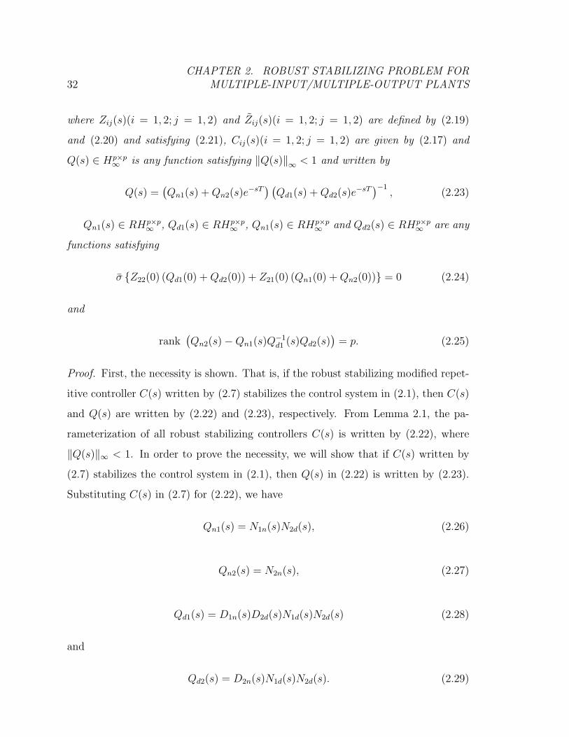
Q(s) ∈ Hp×p∞ is any function satisfying ∥Q(s)∥∞ < 1 and written by
Q(s) =(Qn1(s) +Qn2(s)e
−sT) (
Qd1(s) +Qd2(s)e−sT
)−1, (2.23)
Qn1(s) ∈ RHp×p∞ , Qd1(s) ∈ RHp×p
∞ , Qn1(s) ∈ RHp×p∞ and Qd2(s) ∈ RHp×p
∞ are any
functions satisfying
σ Z22(0) (Qd1(0) +Qd2(0)) + Z21(0) (Qn1(0) +Qn2(0)) = 0 (2.24)
and
rank(Qn2(s)−Qn1(s)Q
−1d1 (s)Qd2(s)
)= p. (2.25)
Proof. First, the necessity is shown. That is, if the robust stabilizing modified repet-
itive controller C(s) written by (2.7) stabilizes the control system in (2.1), then C(s)
and Q(s) are written by (2.22) and (2.23), respectively. From Lemma 2.1, the pa-
rameterization of all robust stabilizing controllers C(s) is written by (2.22), where
∥Q(s)∥∞ < 1. In order to prove the necessity, we will show that if C(s) written by
(2.7) stabilizes the control system in (2.1), then Q(s) in (2.22) is written by (2.23).
Substituting C(s) in (2.7) for (2.22), we have
Qn1(s) = N1n(s)N2d(s), (2.26)
Qn2(s) = N2n(s), (2.27)
Qd1(s) = D1n(s)D2d(s)N1d(s)N2d(s) (2.28)
and
Qd2(s) = D2n(s)N1d(s)N2d(s). (2.29)

2.3. THE PARAMETERIZATION OF ALL ROBUST STABILIZING MODIFIEDREPETITIVE CONTROLLERS FOR MIMO PLANTS 33
Here, N1n(s) ∈ RHp×p∞ , N1d(s) ∈ RHp×p
∞ , N2n(s) ∈ RHp×p∞ , N2d(s) ∈ RHp×p
∞ ,
D1n(s) ∈ RHp×p∞ , D1d(s) ∈ RHp×p
∞ , D1n(s) ∈ RHp×p∞ , D1d(s) ∈ RHp×p
∞ are coprime
factors satisfying
− Z11(s) + Z21(s)C1(s) = D1n(s)D−11d (s), (2.30)
(Z21(s)C2(s) + Z11(s)q(s)− Z21(s)C1(s)q(s)
)D1d(s) = D2n(s)D
−12d (s), (2.31)
(Z12(s)− Z22(s)C1(s)
)D1d(s)D2d(s) = N1n(s)N
−11d (s) (2.32)
and (−Z22(s)C2(s)− Z12(s)q(s) + Z22(s)C1(s)q(s)
)D1d(s)D2d(s)N1d(s) = N2n(s)N
−12d (s). (2.33)
From (2.26)∼(2.29), all of Qn1(s), Qn2(s), Qd1(s) and Qd2(s) are included in RH∞.
Thus, we have shown that if C(s) written by (2.7) stabilize the control system in (2.1)
robustly, Q(s) in (2.22) is written by (2.23). Since q(0) = I, from (2.26)∼(2.29) and
(2.21), (2.24) holds true. In addition, from the assumption of rank C2(s) = p and
from (2.31) and (2.33),
rank D2n(s) = p (2.34)
and
rank N2n(s) = p (2.35)
hold true. From (2.34), (2.35), (2.27) and (2.29), (2.25) is satisfied. We have thus
proved the necessity.
Next, the sufficiency is shown. That is, it is shown that if C(s) and Q(s) ∈ H∞
are settled by (2.22) and (2.23), respectively, then the controller C(s) is written by
34CHAPTER 2. ROBUST STABILIZING PROBLEM FOR
MULTIPLE-INPUT/MULTIPLE-OUTPUT PLANTS
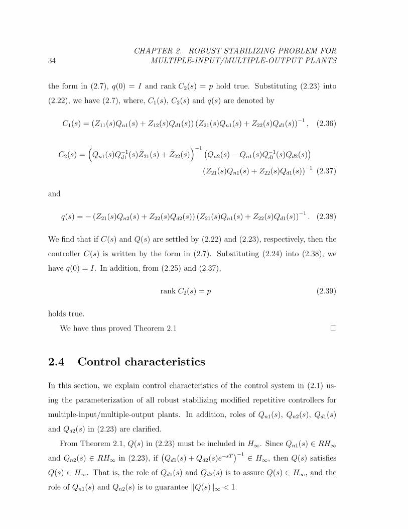
the form in (2.7), q(0) = I and rank C2(s) = p hold true. Substituting (2.23) into
(2.22), we have (2.7), where, C1(s), C2(s) and q(s) are denoted by
C1(s) = (Z11(s)Qn1(s) + Z12(s)Qd1(s)) (Z21(s)Qn1(s) + Z22(s)Qd1(s))−1 , (2.36)
C2(s) =(Qn1(s)Q
−1d1 (s)Z21(s) + Z22(s)
)−1 (Qn2(s)−Qn1(s)Q
−1d1 (s)Qd2(s)
)(Z21(s)Qn1(s) + Z22(s)Qd1(s))
−1 (2.37)
and
q(s) = − (Z21(s)Qn2(s) + Z22(s)Qd2(s)) (Z21(s)Qn1(s) + Z22(s)Qd1(s))−1 . (2.38)
We find that if C(s) and Q(s) are settled by (2.22) and (2.23), respectively, then the
controller C(s) is written by the form in (2.7). Substituting (2.24) into (2.38), we
have q(0) = I. In addition, from (2.25) and (2.37),
rank C2(s) = p (2.39)
holds true.
We have thus proved Theorem 2.1
2.4 Control characteristics
In this section, we explain control characteristics of the control system in (2.1) us-
ing the parameterization of all robust stabilizing modified repetitive controllers for
multiple-input/multiple-output plants. In addition, roles of Qn1(s), Qn2(s), Qd1(s)
and Qd2(s) in (2.23) are clarified.
From Theorem 2.1, Q(s) in (2.23) must be included in H∞. Since Qn1(s) ∈ RH∞
and Qn2(s) ∈ RH∞ in (2.23), if(Qd1(s) +Qd2(s)e
−sT)−1 ∈ H∞, then Q(s) satisfies
Q(s) ∈ H∞. That is, the role of Qd1(s) and Qd2(s) is to assure Q(s) ∈ H∞, and the
role of Qn1(s) and Qn2(s) is to guarantee ∥Q(s)∥∞ < 1.
2.4. CONTROL CHARACTERISTICS 35
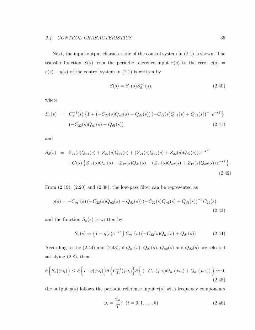
Next, the input-output characteristic of the control system in (2.1) is shown. The
transfer function S(s) from the periodic reference input r(s) to the error e(s) =
r(s)− y(s) of the control system in (2.1) is written by
S(s) = Sn(s)S−1d (s), (2.40)
where
Sn(s) = C−121 (s)
I + (−C22(s)Qn2(s) +Qd2(s)) (−C22(s)Qn1(s) +Qd1(s))
−1 e−sT
(−C22(s)Qn1(s) +Qd1(s)) (2.41)
and
Sd(s) = Z21(s)Qn1(s) + Z22(s)Qd1(s) + (Z21(s)Qn2(s) + Z22(s)Qd2(s)) e−sT
+G(s)Z11(s)Qn1(s) + Z12(s)Qd1(s) + (Z11(s)Qn2(s) + Z12(s)Qd2(s)) e
−sT.
(2.42)
From (2.19), (2.20) and (2.38), the low-pass filter can be represented as
q(s) = −C−121 (s) (−C22(s)Qn2(s) +Qd2(s)) (−C22(s)Qn1(s) +Qd1(s))
−1C21(s),
(2.43)
and the function Sn(s) is written by
Sn(s) =I − q(s)e−sT
C−1
21 (s) (−C22(s)Qn1(s) +Qd1(s)) (2.44)
According to the (2.44) and (2.43), if Qn1(s), Qd1(s), Qn2(s) and Qd2(s) are selected
satisfying (2.8), then
σSn(jωi)
≤ σ
I−q(jωi)
σC−1
21 (jωi)σ(−C22(jωi)Qn1(jωi) +Qd1(jωi))
≃ 0,
(2.45)
the output y(s) follows the periodic reference input r(s) with frequency components
ωi =2π
Ti (i = 0, 1, . . . , ~) (2.46)

36CHAPTER 2. ROBUST STABILIZING PROBLEM FOR
MULTIPLE-INPUT/MULTIPLE-OUTPUT PLANTS
with a small steady state error.
Next, the disturbance attenuation characteristic of the control system in (2.1)
is shown. The transfer function from the disturbance d(s) to the output y(s) of the
control system in (2.1) is written by (2.40). From (2.40), for ωi(i = 0, 1, . . . , ~) in (2.8)
of the frequency component of the disturbance d(s) that is same as that of the periodic
reference input r(s), if (2.45) holds, then the disturbance d(s) is attenuated effectively.
This implies that the disturbance with same frequency component ωi(i = 0, 1, . . . , ~)
of the periodic reference input r(s) is attenuated effectively. That is, the role of Qn2(s)
and Qd2(s) is to specify the disturbance attenuation characteristic for the disturbance
with same frequency component ωi(i = 0, 1, . . . , ~) of the periodic reference input
r(s). When the frequency components of disturbance d(s), ωk(k = 0, 1, · · · , h), are
not equal to ωi(i = 0, 1, · · · , ~), even if
σ I − q(jωk) ≃ 0, (2.47)
the disturbance d(s) cannot be attenuated, because
e−jωkT = 1 (2.48)
and
σI − q(jωk)e
−jωkT
/≃ 0. (2.49)
In order to attenuate the frequency components ωk(k = 0, 1, · · · , h) of the disturbance
d(s), we need to satisfy
σ −C22(jωk)Qn1(jωk) +Qd1(jωk) ≃ 0. (2.50)
This implies that the disturbance d(s) with frequency components ωk = ωi(i =
0, 1, . . . , ~, k = 0, 1, · · · , h) is attenuated effectively. That is, the role of Qn1(s) and
Qd1(s) is to specify disturbance attenuation characteristics for disturbance of frequen-
cy ωd = ωi(i = 0, 1, . . . , ~).
From above discussion, the role of Qn2(s) and Qd2(s) is to specify the input-output
characteristic for the periodic reference input r(s) and to specify for the disturbance

2.5. DESIGN PARAMETERS 37
d(s) of which the frequency component is equivalent to that of the periodic reference
input r(s). The role of Qn1(s) and Qd1(s) is to specify for the disturbance d(s) of
which the frequency component is different from that of the periodic reference input
r(s).
2.5 Design parameters
Generally, the design of the free parameters are using Nyquist stability criterion by
manual examination, which is very difficult and inefficient. To settle this problem, it
is essential to establish an efficiently and easily method for the parameters. In this
section, an efficient design method will be presented for the free parameters based on
the control characteristics and H∞ control approach.
2.5.1 Design parameters for control performance
The objective of this chapter is to develop an efficient design method so that the
closed-loop system in Figure 2.1 is robust stable and has high control precision for
reference input and/or disturbance. Hence, the free parametersQn1(s), Qd1(s), Qn2(s)
and Qd2(s) should be designed after the control characteristics.
First, in order to track the reference input with small steady-state error for fre-
quency components ωi(0, 1, · · · , ~), Qn1(s),Qd1(s), Qn2(s) and Qd2(s) should be set-
tled to satisfy (2.43). That is equal to
σI + (−C22(jωi)Qn2(jωi) +Qd2(jωi)) (−C22(jωi)Qn1(jωi) +Qd1(jωi))
−1 ≃ 0
(2.51)
for all frequency components ωi(0, 1, · · · , ~). Since C22(s) is strictly proper, there
exists C(s) to satisfy
I − C22(0)C(0) = I (2.52)

38CHAPTER 2. ROBUST STABILIZING PROBLEM FOR
MULTIPLE-INPUT/MULTIPLE-OUTPUT PLANTS
and
σ[I − (I − C22(jωi)C(jωi))q(jωi)
]≃ 0, (2.53)
where
q(s) = diag
1
(1 + sτr1), · · · , 1
(1 + sτrp)
, (2.54)
Qn2(s) = C(s)Qd2(s) ∈ RH∞ (2.55)
and
Qd2(s) = −q(s) −C22(s)Qn1(s) +Qd1(s) . (2.56)
Then, the low-pass filter q(s) can be written as
q(s) = C−121
(I − C22(s)C(s)
)q(s)C21(s). (2.57)
Obviously, C(s) = 0 satisfies (2.52), (2.53) and (2.55), and q(s) = q(s).
On the other hand, to attenuate the frequency components ωk(0, 1, · · · , h) effec-
tively, Qn1(s) is settled by
Qn1(s) = C−122o(s)Qd1(s)qd(s), (2.58)
where C22o(s) ∈ RH∞ is an outer function of C22(s) satisfying
C22(s) = C22i(s)C22o(s), (2.59)
C22i(s) ∈ RH∞ is an inner function satisfying C22i(0) = I and σ C22i(jω) = 1(∀ω ∈
R+), qd(s) is a low-pass filter satisfying qd(0) = I, as
qd(s) = diag
1
(1 + sτd1)αd1
, · · · , 1
(1 + sτdp)αdp
(2.60)
is valid, αdi(i = 1, . . . , p) are arbitrary positive integers to make C−122o(s)qd(s) proper
and τdk ∈ R(k = 1, . . . , p) are any positive real numbers satisfying
σ I − C22i(jωk)qd(jωk) ≃ 0 (2.61)
for ωk(0, 1, · · · , h).

2.5. DESIGN PARAMETERS 39
2.5.2 Design parameters for robust stability conditions
From Theorem 2.1, the free parameters Qn1(s), Qd1(s), Qn2(s) and Qd2(s) are re-
quired to satisfy the robust stability conditions Q(s) ∈ H∞ and ∥Q(s)∥∞ < 1. For
convenience, choose the C(s) = 0 and Qd1(s) ∈ RH∞ and substitute (2.58), (2.56)
and (2.55) into (2.23) leading to
Q(s) = C−122o(s)qd(s)
I − q(s)q(s)e−sT
−1
, (2.62)
where
q(s) = I − C22i(s)qd(s). (2.63)
Note that
∥q(s)∥∞ < 1, (2.64)
since C22i(s)qd(s) works as low-pass filter. According to H∞ control approach, the
conditions Q(s) ∈ H∞ and ∥Q(s)∥∞ < 1 are the robust stability conditions of closed-
loop system in Figure 2.3, where ∆(s) is an uncertainty satisfying ∥∆(s)∥∞ = 1.
qê(s)qö(s)eàsT
Cà122o(s)qöd(s)
Éê (s)
+
y1(s)u1(s)
u2(s) y2(s)
Qd(s)
+
Figure 2.3: Closed-loop system for Q(s) ∈ H∞ and ∥Q(s)∥∞ < 1
Since C−122o(s)qd(s), q(s) and q(s) are RH∞, if (I + q(s)q(s)e−sT )−1 ∈ H∞, then
Q(s) ∈ H∞ holds. In fact, the (I + q(s)q(s)e−sT )−1 ∈ H∞ is equivalent that the
closed-loop system Qd(s) is stable. Due to ∥e−sT∥∞ ≤ 1, according to the small gain

40CHAPTER 2. ROBUST STABILIZING PROBLEM FOR
MULTIPLE-INPUT/MULTIPLE-OUTPUT PLANTS
theorem, the stability condition is
∥q(s)q(s)∥∞ < 1. (2.65)
Because of ∥q(s)∥∞ ≤ 1 and ∥q(s)∥∞ < 1, the stability condition for Qd(s) is satisfied.
That means Q(s) ∈ H∞.
From the Figure 2.3, the system can be represented as y(s) = T (s)u(s)
u(s) = Λ(s)y(s), (2.66)
where y(s) =[yT1 (s) yT2 (s)
]T, u(s) =
[uT1 (s) uT
2 (s)]T
, the transfer function
T (s) is written by
T (s) =
C−122o(s)qd(s) C−1
22o(s)qd(s)
q(s)q(s) q(s)q(s)
(2.67)
and the uncertainties Λ(s) is written as
Λ(s) =
∆ 0
0 e−sT
. (2.68)
Note that ∥Λ(s)∥∞ ≤ 1, then the robust stability condition ∥Q(s)∥∞ < 1 is equivalent
to the condition ∥∥∥∥∥∥ C−1
22o(s)qd(s) C−122o(s)qd(s)
q(s)q(s) q(s)q(s)
∥∥∥∥∥∥∞
< 1, (2.69)
and further it as ∥∥∥∥∥∥ C−1
22o(s)qd(s) 0
0 q(s)q(s)
∥∥∥∥∥∥∞
<1
2. (2.70)
This condition shows that, for given C22o(s), we should chose suitable low-pass filters
q(s) and qd(s) to satisfy robust stability conditions.
According to the design method for C22i(s) and C22o(s) in [102], C22o(s) must be
strictly proper. We found that there exist the bandwidth restrictions for qd(s) and

2.5. DESIGN PARAMETERS 41
q(s) in (2.70). Without loss of generality, to explain this problem clearly and simply,
we set C22o(s) as
C22o(s) =β
1 + α s, α > 0. (2.71)
Since C−122o(s)qd(s) is proper, we will analysis it in two cases for
qd(s) =1
1 + τd s(2.72)
and
qd(s) =1
(1 + τd s)2, (2.73)
respectively.
Case 1 The low-pass filter qd(s) is selected in (2.72), the infinity norm of C−122o(s)qd(s)
is
∥C−122o(s)qd(s)∥∞ = max
ω∈R
∣∣∣∣ 1 + j α ω
β (1 + j τd ω)
∣∣∣∣ = maxω∈R
1
|β|
√1 + α2 ω2
1 + τ 2d ω2
. (2.74)
Then, according to (2.70), when we choose α < τd, the inequality
1
|β|<
1
2(2.75)
must be satisfied, or when we choose α > τd, the inequality
α
τd<
|β|2
(2.76)
must be satisfied. These two conditions means that the restriction of the cutoff
frequency ωdc for low-pass filter qd(s) is that
ωdc =1
τd< max
1
α,|β|2α
. (2.77)
Case 2 The low-pass filter qd(s) is selected in (2.73), the infinity norm of C−122o(s)qd(s)
is
∥C−122o(s)qd(s)∥∞ = max
ω∈R
∣∣∣∣ 1 + j α ω
β (1 + j τd ω)2
∣∣∣∣ = maxω∈R
1
|β|
√1 + α2 ω2
1 + τ 2d ω2
. (2.78)

42CHAPTER 2. ROBUST STABILIZING PROBLEM FOR
MULTIPLE-INPUT/MULTIPLE-OUTPUT PLANTS
Then, according to (2.70), when we choose
√2
2α < τd, the inequality
1
|β|<
1
2(2.79)
must be satisfied, or when we choose
√2
2α > τd and the condition (2.79) holds,
the inequality
√2α
2
√β2 −
√β4 − 4 β2
β2< τd <
√2α
2
√β2 +
√β4 − 4 β2
β2(2.80)
must be stratified. Obviously, there is no low-pass filter qd(s) in the form of
(2.60) for
1
|β|≥ 1
2(2.81)
in this case. From above discussion, the restriction of the cutoff frequency ωdc
for low-pass filter qd(s) is that
ωdc =1
τd< max
√2
α,
√2α
2
√β2 −
√β4 − 4 β2
β2
−1 . (2.82)
with (2.79) in this case.
The results in these two cases show that we would better to choose the qd(s) to
make C−122o(s)qd(s) biproper. Furthermore, there exists the bandwidth restriction for
the low-pass filter qd(s).
On the other hand, the restriction of the cutoff frequency ωc for the low-pass filter
q(s) has been detailed in [29]. This subsection demonstrates that when choose the
low-pass filter for the perfect control performance, the robust stability condition may
be not guaranteed. That results in tradeoff problem for modified repetitive control
system design.

2.5. DESIGN PARAMETERS 43
2.5.3 Robust stability condition based on linear matrix in-
equalities (LMIs)
The computation of the infinity norm is complicated and requires a search. Control
engineering interpretation of the infinity norm is the distance in the complex plane
form the origin to the farthest point on the Nyquist plot, and it also appears as the
peak value on the Bode magnitude plot. However, the graphical method can lead to
a wrong answer for a lightly damped system if the frequency gride is not sufficiently
dense [103]. Moreover, the robust stability condition (2.70) has conservativeness. To
compute the infinity norm easily and reduce the conservativeness, the Bounded Real
Lemma (BRL) [104] based on linear matrix inequality is employed.
Assume the sate-space description of C−122o(s)qd(s) and q(s)q(s) are
C−122o(s)qd(s) =
Ao Bo
Co Do
(2.83)
and
q(s)q(s) =
Ah Bh
Ch 0
. (2.84)
Then, from Figure 2.3, the the state-space description of Q(s) can be achieved as xq(s) = Aqxq(t) + Adxq(t− T )(t) +Bqu1(t)
y1(t) = Cqxq(t) + Cdxq(t− T ) +Dqu1(t), (2.85)
where
Aq =
Ao 0
0 Ah
, Ad =
0 BoCh
0 BhCh
, Bq =
Bo
Bh
,
Cq =[Co 0
], Cd =
[0 DoCh
]and Dq = Do.
To obtain the stability condition for ∥Q(s)∥∞ < 1, the following result is required.

44CHAPTER 2. ROBUST STABILIZING PROBLEM FOR
MULTIPLE-INPUT/MULTIPLE-OUTPUT PLANTS
Consider a nominal system Gn(s) with time-varying delay given by
Gn(s) :
x(t) = Ax(t) + Adx(t− τ(t)) +Bϖϖ(t)
z(t) = Cx(t) + Cdx(t− τ(t)) +Dϖϖ(t)
x(t) = ϕ(t), t ∈ [τ , 0]
, (2.86)
where the initial condition, ϕ(t), is a continuous vector-valued initial function of
t ∈ [τ , 0], τ(t) is a time delay and satisfying
0 ≤ τ(t) ≤ τ , |τ(t)| ≤ d < 1, t ≥ 0. (2.87)
The H∞ performance of Gn(s), i.e.,
∥Gn(s)∥∞ < γ, γ > 0 (2.88)
is obtained by solving the following feasible problem.
Lemma 2.2 (BRL [104]). Given scalars τ , γ and d > 0, if there exist matrices Z, S,
M , Q22 and P11 > 0, Q11 and P22 ≥ 0, and any matrices Q12 and P12 with appropriate
dimensions such that the following LMIs hold
Ω1 =
Ω11 Ω12 Ω13 Ω14 CT τATQ22 dP12 0
∗ Ω22 Ω23 0 CTd τAT
dQ22 0 dP22
∗ ∗ Ω33 Ω34 0 0 0 0
∗ ∗ ∗ −γ2I DTϖ τBT
ϖQ22 0 0
∗ ∗ ∗ ∗ −I 0 0 0
∗ ∗ ∗ ∗ ∗ −Q22 0 0
∗ ∗ ∗ ∗ ∗ ∗ −dS 0
∗ ∗ ∗ ∗ ∗ ∗ ∗ −dZ
< 0, (2.89)
Q11 Q12
∗ Q2
≥ 0 (2.90)
and P11 P12
∗ P22
≥ 0, (2.91)

2.5. DESIGN PARAMETERS 45
where
Ω11 = M −Q22 + τ 2(Q11 +Q12A+ ATQT
12
)+ P12 + P T
12 + P11A+ ATP T11,
Ω12 = Q22 + τ 2Q12Ad + P11Ad − P12,
Ω13 = ATP12 + P T22 −QT
12,
Ω14 = P11Bϖ + τ 2Q12Bϖ,
Ω22 = dS − (1− d)M −Q22,
Ω23 = ATdP12 − P22 +QT
12,
Ω33 = dZ −Q11
and
Ω34 = P T12Bϖ,
then system (2.86) is asymptotically stable.
Applying this Lemma to the system (2.85) with d = 0 and τ = T , the robust
stability conditions Q(s) ∈ H∞ and ∥Q(s)∥∞ < 1 are given in form of LMIs.
Theorem 2.2. Given scalars T and γ = 1, if there exist matrices M , Q22 and
P11 > 0, Q11 and P22 ≥ 0, and any matrices Q12 and P12 with appropriate dimensions
such that (2.90), (2.91) and the following LMI hold
Ξ11 Ξ12 Ξ13 Ξ14 CT TATq Q22
∗ Ξ22 Ξ23 0 CTd TAT
dQ22
∗ ∗ −Q11 P T12Bq 0 0
∗ ∗ ∗ −γ2I DTq TBT
q Q22
∗ ∗ ∗ ∗ −I 0
∗ ∗ ∗ ∗ ∗ −Q22
< 0, (2.92)
where
Ξ11 = M −Q22 + T 2(Q11 +Q12Aq + AT
dQT12
)+ P12 + P T
12 + P11Aq + ATq P
T11,
46CHAPTER 2. ROBUST STABILIZING PROBLEM FOR
MULTIPLE-INPUT/MULTIPLE-OUTPUT PLANTS
Ξ12 = Q22 + T 2Q12Ad + P11Ad − P12,
Ξ13 = ATq P12 + P T
22 −QT12,
Ξ14 = P11Bq + T 2Q12Bq,
Ξ22 = −M −Q22
and
Ξ23 = ATdP12 − P22 +QT
12,
then system (2.85) is asymptotically stable.
Finally, according to above discussions, a design procedure of robust stabilizing
modified repetitive controller C(s) satisfying Theorem 2.1 is summarized as follows:
Procedure
1. Obtain C11(s), C12(s), C21(s) and C22(s) by solving the robust stability problem
using the Riccati equation based H∞ control.
2. Settle the free parameters Qn1(s), Qd1(s), Qn2(s) and Qd2(s) as shown in Sub-
section 2.5.1.
3. According to Subsection 2.5.2, choose appropriate parameters τri, τdi and αdi(i =
1, · · · , p) for the low-pass filters q(s) and qd(s) to satisfy (2.51), (2.61) and The-
orem 2.2.
2.6 Numerical example
In this section, numerical examples are made to illustrate the validity of the pro-
posed approach. Consider the problem to obtain the parameterization of all robust
stabilizing modified repetitive controllers for the set of plants G(s) written by (2.3),

2.6. NUMERICAL EXAMPLE 47
where
Gm(s) =
s+ 3
(s− 2)(s+ 9)
2
(s− 2)(s+ 9)
s+ 3
(s− 2)(s+ 9)
s+ 4
(s− 2)(s+ 9)
(2.93)
and
WT (s) =s+ 400
550. (2.94)
The period T of the periodic reference input r is given by T = 10[sec].
Solving the robust stability problem using Riccati equation based H∞ control
as Theorem 2.1, the parameterization of all robust stabilizing controllers C(s) is
obtained. In addition, we find that C22(s) is of minimum phase as
C22(s) =
−434
s+ 408
347
s+ 408347
s+ 408
434
s+ 408
. (2.95)
Since C22(s) is of minimum phase, we set Qn1(s), Qn2(s), Qd1(s) and Qd2(s) in
(2.23) as
Qd1(s) = I ∈ RH∞, (2.96)
Qn1(s) = C−122 (s)qd(s) ∈ RH∞, (2.97)
Qn2(s) = 0 ∈ RH∞, (2.98)
and
Qd2(s) = −q(s) (I − qd(s)) ∈ RH∞, (2.99)
where q(s) and q(s) are written by
qd(s) =
1
0.002 s+ 10
01
0.002 s+ 1
(2.100)

48CHAPTER 2. ROBUST STABILIZING PROBLEM FOR
MULTIPLE-INPUT/MULTIPLE-OUTPUT PLANTS
and
q(s) =
1
0.002 s+ 10
01
0.002 s+ 1
. (2.101)
Using Qd1(s) in (2.96) and Qd2(s) in (2.99), Theorem 2.2 has feasible solutions and
the H∞ performance index γ is 0.904, i.e., ∥Q(s)∥∞ < 0.904. To verify this result,
0 0.5 1 1.5 2 2.5 3 3.5 4−2
−1.5
−1
−0.5
0
0.5
1
1.5
2
Im
Re
Figure 2.4: The nyquist plot of det(Qd1(s) +Qd2(s)e−sT )
the Nyquist plot of det(Qd1(s) + Qd2(s)e−sT ) and the largest singular value plot of
Q(s) are shown in Figure 2.4 and Figure 2.5, respectively. Since the Nyquist plot of
det(Qd1(s) + Qd2(s)e−sT ) does not encircle the origin, we find that Q(s) in (2.23) is
included in H∞. Figure 2.5 illustrates σQ(jω) ≃ 0.9 < 1(∀ω ∈ R), i.e., ∥Q(s)∥∞ ≃
0.9 < 1.
According to analysis result in Subsection 2.5.2, there exists the bandwidth lim-
itation for low-pass filter qd(s). To verify this result, we draw the Nyquist plot of
det(Qd1(s)+Qd2(s)e−sT ) and the largest singular value plot of Q(s) when τd 1,2 = 0.001
in Figure 2.6 and Figure 2.7. There is no feasible solution for LMIs-constraint con-

2.6. NUMERICAL EXAMPLE 49
10−10
10−5
100
105
1010
0.7
0.75
0.8
0.85
0.9
0.95
Frequency[rad/sec]
Lar
ges
t si
ngula
r val
ue
Figure 2.5: Largest singular value plot of Q(s)
ditions in Theorem 2.2 and the H∞ performance index γ is 1.825, which means
∥Q(s)∥∞ < 1.825. And Figure 2.6 shows that Q(s) ∈ H∞. This verifies that the
design method make Q(s) belong to H∞ for arbitrary low-pass filters q(s) and qd(s).
However, Fiure 2.7 shows that σQ(jω) ≃ 1.8 > 1(∀ω ∈ R), i.e., ∥Q(s)∥∞ > 1. This
result demonstrates that there exists some restriction on the bandwidth. Therefore,
when choose the low-pass filters to obtain high control precision, the robust stability
must be guaranteed.
Using above-mentioned parameters, we have a robust stabilizing modified repeti-
tive controller. When ∆(s) is given by
∆(s) =
s− 100
s+ 500
−100
s+ 500−200
s+ 500
s− 100
s+ 500
, (2.102)
in order to confirm that ∆(s) satisfies (2.4), the largest singular value plot of ∆(s)
and the gain plot of WT (s) are shown in Figure 2.8. Here, the solid line shows the
gain plot of WT (s) and the dashed line shows that of ∆(s). Figure 2.8 shows that the

50CHAPTER 2. ROBUST STABILIZING PROBLEM FOR
MULTIPLE-INPUT/MULTIPLE-OUTPUT PLANTS
0.5 1 1.5 2 2.5−1
−0.8
−0.6
−0.4
−0.2
0
0.2
0.4
0.6
0.8
1
Figure 2.6: The nyquist plot of det(Qd1(s) +Qd2(s)e−sT ) when τd 1,2 = 0.001
10−10
10−5
100
105
1010
0.8
1
1.2
1.4
1.6
1.8
2
Frequency[rad/sec]
Lar
ges
t si
ng
ula
r v
alu
e
Figure 2.7: Largest singular value plot of Q(s) when τd 1,2 = 0.001
uncertainty ∆(s) in (2.102) satisfies (2.4).
When the designed robust stabilizing modified repetitive controller C(s) is used,

2.6. NUMERICAL EXAMPLE 51
10−10
10−5
100
105
1010
−20
0
20
40
60
80
100
120
140
160
Frequency[rad/sec]
Gai
n[dB
]
W
T(s)
∆(s)
Figure 2.8: Largest singular value plot of ∆(s) and gain plot of WT (s)
the response of the error e(t) = r(t)− y(t) in (2.1) written by
e(t) =
e1(t)
e2(t)
=
r1(t)− y1(t)
r2(t)− y2(t)
(2.103)
for the periodic reference input r
r(t) =
r1(t)
r2(t)
=
sin(2πT t
)2 sin
(2πT t
) (2.104)
is shown in Figure 2.9. Here, the broken line shows the response of the periodic
reference input r1(t), the dotted line shows that of the periodic reference input r2(t),
the solid line shows that of the error e1(t), and the dotted and broken line shows that
of the error e2(t). Figure 2.9 shows that the output y(t) follows the periodic reference
input r(t) with small steady state error.
Next, using the designed the robust stabilizing modified repetitive controller C(s),
the disturbance attenuation characteristic is shown. The response of the output y(t)

52CHAPTER 2. ROBUST STABILIZING PROBLEM FOR
MULTIPLE-INPUT/MULTIPLE-OUTPUT PLANTS
0 5 10 15 20 25 30 35 40−2
−1.5
−1
−0.5
0
0.5
1
1.5
2
t[sec]
r 1(t),
r 2(t),
e 1(t),
e 2(t)
Figure 2.9: Response of the error e(t) for the reference input r(t)
written by
y(t) =
y1(t)
y2(t)
(2.105)
for the disturbance d(t) of which the frequency component is equivalent to that of
the periodic reference input r(t)
d(t) =
d1(t)
d2(t)
=
sin(2πT t
)2 sin
(2πT t
) (2.106)
is shown in Figure 2.10. Here, the broken line shows the response of the disturbance
d1(t), the dotted line shows that of the disturbance d2(t), the solid line shows that of
the output y1(t) and the dotted and broken line shows that of the output y2(t). Figure
2.10 shows that the disturbance d(t) is attenuated effectively. Finally, the response of
the output y(t) for the disturbance d(t) of which the frequency component is different

2.6. NUMERICAL EXAMPLE 53
0 5 10 15 20 25 30 35 40−2
−1.5
−1
−0.5
0
0.5
1
1.5
2
t[sec]
d 1(t),
d 2(t),
y 1(t),
y 2(t)
Figure 2.10: Response of the output y(t) for the disturbance d(t)
from that of the periodic reference input r(t)
d(t) =
d1(t)
d2(t)
=
sin(πT t
)2 sin
(πT t
) (2.107)
is shown in Figure 2.11. Here, the broken line shows the response of the disturbance
d1(t), the dotted line shows that of the disturbance d2(t), the solid line shows that
of the output y1(t) and the dotted and broken line shows that of the output y2(t).
Figure 2.11 shows that the disturbance d(t) is attenuated effectively.
A robust stabilizing modified repetitive controllers can be easily designed in the
way shown here. The design method proposed in this chapter simplifies the design
process which does not need to draw the Nyquist plot and the largest singular value
plot of free parameter Q(s) simultaneously. The simulation result show that this
modified repetitive control system can be used to track or attenuate the signals with
different period time.

54CHAPTER 2. ROBUST STABILIZING PROBLEM FOR
MULTIPLE-INPUT/MULTIPLE-OUTPUT PLANTS
0 10 20 30 40 50 60 70 80−2
−1.5
−1
−0.5
0
0.5
1
1.5
2
t[sec]
d 1(t),
d 2(t),
y 1(t),
y 2(t)
Figure 2.11: Response of the output y for the disturbance d(t)
2.7 Conclusions
In this chapter, we gave a complete proof of the theorem for the parameterization
of all robust stabilizing modified repetitive controllers for multiple-input/multiple-
output plants omitted in [73] and showed effectiveness of the parameterization of all
robust stabilizing modified repetitive controllers for multiple-input/multiple-output
plants. We clarified control characteristics using the parameterization in [73]. The
design of free parameters guarantees the perfect tracking performance and/or good
disturbance attenuation characteristics for different period-time. Viewing the time-
delay element as an uncertainty and applying H∞ control approach, there exists the
bandwidth limitation of low-pass filter for specify the disturbance characteristic for
both minimum phase and non-minimum phase control plant. In order to simplify the
design process and avoid the wrong results obtained by graphical method, the robust
stability conditions are converted into LMIs-constraint conditions by employing the

2.7. CONCLUSIONS 55
delay-dependent bounded real lemma. This work can be extended to solve the tradeoff
problem. In addition, a design procedure using the parameterization was presented.
Finally a numerical example was illustrated to show the effectiveness of the proposed
method. Using the result in this paper, we can easily design a robust stabilizing
modified repetitive controller.

57
Chapter 3
Robust Stabilizing Problem for
Time-varying periodic Signals
3.1 Introduction
In practical applications, many control systems must deal with periodic reference
and/or disturbance signals, for example industrial robots, computer disk drives, CD
player tracking control, machine tool motion control, and vibration attenuation of en-
gineering structures. One control system that can deal with periodic reference and/or
disturbance signals is a repetitive control system, as proposed by Hara et al. [28]. A
disadvantage of typical repetitive controllers is that they are based on the constant
period of the external signal. This means that in practical applications, either the
period must be constant (±0.1%) or an accurate measurement of the periodicity is
necessary.
However, in practice, rotary motion systems have found applications in various
industry products. For most applications, the systems are required to operate at
variable speeds while following repetitive trajectories and/or rejecting disturbances,
such as the brushless DC electric motor in a typical laser printer described by Chen et
al. [101]. In general, the periods of reference signals and/or disturbances are mostly
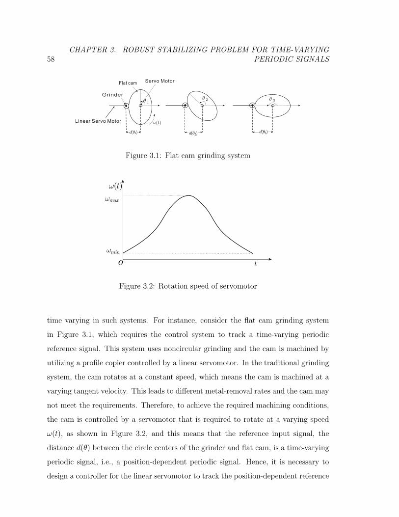
58CHAPTER 3. ROBUST STABILIZING PROBLEM FOR TIME-VARYING
PERIODIC SIGNALS
d(ò1) d(ò2) d(ò3)
ò 1ò 2 ò 3
Flat cam
Grinder
Linear Servo Motor
Servo Motor
!(t)
Figure 3.1: Flat cam grinding system
t
!(t)
!min
!max
o
Figure 3.2: Rotation speed of servomotor
time varying in such systems. For instance, consider the flat cam grinding system
in Figure 3.1, which requires the control system to track a time-varying periodic
reference signal. This system uses noncircular grinding and the cam is machined by
utilizing a profile copier controlled by a linear servomotor. In the traditional grinding
system, the cam rotates at a constant speed, which means the cam is machined at a
varying tangent velocity. This leads to different metal-removal rates and the cam may
not meet the requirements. Therefore, to achieve the required machining conditions,
the cam is controlled by a servomotor that is required to rotate at a varying speed
ω(t), as shown in Figure 3.2, and this means that the reference input signal, the
distance d(θ) between the circle centers of the grinder and flat cam, is a time-varying
periodic signal, i.e., a position-dependent periodic signal. Hence, it is necessary to
design a controller for the linear servomotor to track the position-dependent reference

3.1. INTRODUCTION 59
input signal d(θ). Because it is periodic with respect to angular position, but not
necessarily with respect to time, the conventional repetitive control technique is not
directly applicable in this case. A very common design method for this class of system
is to transform a linear system from the time domain into a spatial domain.
Recently, several studies have considered the problem of rejecting and/or tracking
spatially periodic disturbances and/or reference inputs for rotary motion systems
using a spatial-based repetitive controller [105, 106, 107, 108, 109, 110]. Nakano et
al. [105] eliminated the angular position-dependent disturbances in constant-speed
rotation control systems by transforming all signals defined in the time domain to the
spatial domain, and obtained a stabilizing controller using coprime factorization. To
track spatially periodic reference inputs, Mahawan and Luo [106] proposed a repetitive
controller design method using operator-theoretic approaches. Sun [107] addressed
the tracking or rejecting problem for position-dependent signals by converting the
continuous-time system into a discrete spatial system. A more advanced design based
on linearization using H∞ robust control was proposed by Chen and Allebach [108].
Chen and Chiu [109] proved that the reformulated nonlinear plant model could be
cast into a quasilinear parameter-varying system that can be used to address spatially
periodic disturbances. In particular, a method of designing a spatial-based repetitive
control system for rotary motion systems subject to position-dependent disturbances
based on adaptive feedback linearization was presented by Chen and Yang [110].
With the domain transformation, the linear system in the time domain is cast into
a nonlinear system in the spatial domain. Before designing the repetitive controller,
it is necessary to linearize the nonlinear control system, which makes the design of the
repetitive controller more complicated and difficult. In particular, for the control of
plants with uncertainties or time-varying state delay, there exists a trade-off problem
between robust stability and control performance in the design of repetitive control
systems, and spatial-based design methods do not provide a satisfactory solution to
this trade-off. Hence, there is a clear need to develop an efficient design method for

60CHAPTER 3. ROBUST STABILIZING PROBLEM FOR TIME-VARYING
PERIODIC SIGNALS
repetitive control systems that track or reject the position-dependent signals.
In this chapter, the position-dependent signal will be converted into a time-varying
periodic signal. Inspired by the structure of the repetitive controller[28] and the struc-
ture of the optimal repetitive controller[38], we propose a new modified repetitive
controller for position-dependent signals. Compared with the conventional modified
repetitive controller, the constant time-delay element is replaced by a time-varying
operator in our new controller. Moreover, an adjustable parameter is introduced in
the new structure to adjust the convergence rate of the closed-loop system and im-
prove the control precision. This controller is plugged into the closed-loop system for
a strictly proper plant with uncertainties to reject position-dependent disturbances.
The control performance of this repetitive control system then depends heavily on
the cutoff frequency of the low-pass filter and the adjustable parameter that represent
the trade-off between system robust stability and rejection performance. To achieve
the optimal performance and guarantee robust stability, the design problem consid-
ered in this paper is converted into a robustly stabilizing problem based on linear
matrix inequalities (LMIs). Two LMI-based robust stability conditions of the closed-
loop system with time-varying state delay are derived for fixed parameters. One is
a delay-dependent robust stability condition that is derived based on the free-weight
matrix. The other robust stability condition is based on the H∞ control approach
and introduces a linear unitary operator. The optimal values of the cutoff frequency
of the low-pass filter and the adjustable parameter can be obtained by solving the op-
timization problems with LMI-constrained conditions. Finally, a numerical example
is provided to demonstrate the effectiveness of the proposed design method.
3.2 Problem statement and preliminaries
In this section, we will transform the position-dependent signal into a time-varying
periodic signal and establish a new structure of modified repetitive controller.

3.2. PROBLEM STATEMENT AND PRELIMINARIES 61
First, we convert the position-dependent reference into a time-varying periodic
signal, in contrast with the conventional processing method, which transforms a lin-
ear system in the time domain into a nonlinear system in the spatial domain. The
position-dependent disturbance d(t) is given by
d(t) := d(θ) = d(θ − Tθ), (3.1)
where d(θ) is the position-dependent disturbance, Tθ is the period, and the rotational
angle θ(t) is defined as: θ(t) := f(t) =∫ t
0ω(s)ds
ω(t) = dθdt
> 0 ∀ t > 0, (3.2)
where ω(t) is the rotational speed and guarantees that θ(t) is strictly monotonic such
that t = f−1(θ) exists. Thus, for a large enough t, there exist a tθ > 0 such that
f(tθ) = f(t)− Tθ. We define a time-varying function τ(t) as
τ(t) :=
t0 0 < t < t0
t− f−1(f(t)− Tθ) = t− tθ t ≥ t0
, (3.3)
where t0 = f−1(Tθ) satisfies Tθ = f(t0) − f(0). Then by Lagrange’s mean value
theorem, there exists at least one point ξ ∈ (tθ, t) such that
Tθ = f(t)− f(tθ) = f ′(ξ)τ(t) = ω(ξ)τ(t). (3.4)
Then
τ(t) =Tθ
ω(ξ)≤ Tθ
ωmin
. (3.5)
From the inverse function theorem, the derivative of function τ(t) is
τ(t) =
0 0 < t < t0
1− ω(t)ω(tθ)
≤ 1− ωminωmax
t ≥ t0
. (3.6)
From the equations (3.5) and (3.6), there exist positive scalars τ and µ such that
τ(t) satisfies
0 < τ(t) ≤ τ , τ(t) ≤ µ, 0 ≤ µ < 1. (3.7)

62CHAPTER 3. ROBUST STABILIZING PROBLEM FOR TIME-VARYING
PERIODIC SIGNALS
Then, the position-dependent disturbance signal can be transformed into a time-
varying periodic signal as
d(t) =
d(θ(t)) 0 < t < t0
d(t− τ(t)) t ≥ t0
, (3.8)
where τ(t) is the period defined in (3.3) and satisfying (3.7).
Q(s)Dü
à
aI
Figure 3.3: The new repetitive control system
Given the time-varying period and inspired by the structure of repetitive controllers[28]
and optimal repetitive controllers[38], we establish a new repetitive controller, shown
in Figure 3.3, for time-varying periodic signals. Compared with the conventional
repetitive controller, the constant time-delay element is replaced by the time-varying
operator Dτ defined as
Dτ (v(t)) := v(t− τ(t)), (3.9)
where τ(t) is the period of the disturbance d(t) in (3.8).
It is well known that the performance of a repetitive control system depends
strongly on the cutoff frequency of the included low-pass filter, which represents
the trade-off between system stability and control precision. However, it is hard to
determine the optimal bandwidth in practice because of the plant uncertainty and
system stability. To overcome this problem, we modify the system gain by introducing
an adjustable parameter a into the repetitive controller. From the structure of the
repetitive controller in Figure 3.3, the gain of CRM(s) is always proportional to the
adjustable parameter a; thus, the performance of the repetitive control system is

3.2. PROBLEM STATEMENT AND PRELIMINARIES 63
strongly dependent on both the cutoff frequency ωc and the adjustable parameter a.
Hence, it is clear that the cutoff frequency ωc and the adjustable parameter a should
be as high as possible to obtain good rejection.
We consider the design problem of the modified repetitive control system shown
in Figure 3.4 that rejects signals that are periodic in the spatial domain while the
rotational speed varies in real-time. The strictly proper plant with uncertainties is
)(tr )(te
)(txr
pF
)(tB p
)(tu )(tx p&
Is
1
)(tAp
)(txp
pC)(ty)(sCRM
)( sG
à
++ ++
aI+
++
! cIs
1Dü +
à
Q(s)
)(txr&
wD)(td
)(tyr
Figure 3.4: The repetitive control system with uncertainties
described as xp(t) = Ap(t)xp(t) +Bp(t)u(t) +Dwd(t)
y(t) = Cpxp(t), (3.10)
where xp(t) ∈ Rn, u(t) ∈ Rm, and y(t) ∈ Rm are the state, input, and output signals,
respectively, Ap(t) ∈ Rn×n, Bp(t) ∈ Rn×m, Cp ∈ Rm×n, and Dw ∈ Rn×m. d(t) ∈ Rm is
an input disturbance that is periodic in the spatial domain and belongs to L2[0, tf ].
Assume that the uncertainties of the plant are given by[Ap(t) Bp(t)
]=
[Ap +∆Ap(t) Bp +∆Bp(t)
][∆Ap(t) ∆Bp(t)
]= ΦpΓ(t)
[ΨA ΨB
] , (3.11)
where Ap ∈ Rn×n, Bp ∈ Rn×m, Φp, ΨA, and ΨB are known constant matrices, and
Γ(t) ∈ Rn×n is an unknown real and possibly time-varying matrix with Lebesgue-
measurable entries satisfying
ΓT (t)Γ(t) ≤ I, ∀t ≥ 0. (3.12)
Q(s), given by
Q(s) =ωc
s+ ωc
I ∈ Rm×m, (3.13)

64CHAPTER 3. ROBUST STABILIZING PROBLEM FOR TIME-VARYING
PERIODIC SIGNALS
is the low-pass filter of the repetitive controller CRM(s), where ωc is the cutoff fre-
quency of the low-pass filter Q(s), and a is an adjustable parameter.
The problem that should be addressed first is to design a feedback controller of
the form
u(t) = Fpxp(t) + e(t) (3.14)
such that the closed-loop system, without the modified repetitive controller, is stabi-
lized. Applying the control law (3.14) to (3.10) with r(t) ≡ 0 yields the closed-loop
system x(t) = Ap(t)−Bp(t)Cp +Bp(t)Fpxp(t) +Dwd(t)
y(t) = Cpxp(t)
. (3.15)
The following lemma presents a rate-dependent state-feedback controller to stabilize
(3.15) robustly with a prescribed H∞ norm-bound specification.
Lemma 3.1. [111] For a prescribed scalar γ > 0, the closed-loop system (3.15) is
robustly stable and satisfies ∥y(t)∥2 < γ∥d(t)∥2, if there exist a matrix P T = P > 0,
a scalar λ > 0, and an arbitrary matrix W with appropriate dimensions satisfying
Λ1 Dw PCTp Λ2 λΦ
∗ −I 0 0 0
∗ ∗ −γ2I 0 0
∗ ∗ ∗ −λI 0
∗ ∗ ∗ ∗ −λI
< 0, (3.16)
Λ1 := (Ap −BpCp)P +BpW +W TBTp + P (Ap −BpCp)
T , (3.17)
and
Λ2 := PΨTA − PCT
p ΨTB +W TΨT
B. (3.18)
Then the H∞ state-feedback controller is given by Fp = WP−1.
The scalar γ can be regarded as a disturbance performance index. The problem
of robust stabilization, to find a state-feedback controller such that the closed-loop

3.3. ROBUST STABILITY CONDITIONS 65
system is stable with disturbance attenuation γ, can easily be obtained by solving
the above feasible problem for the given γ.
We next present an efficient method to find the optimal values of the cutoff fre-
quency ωc and the adjustable parameter a.
3.3 Robust stability conditions
In this section, we describe a design method to find the optimal values of the cutoff
frequency of the low-pass filter and the adjustable parameter.
As shown in Figure 3.4, the state-space description of the repetitive controller isxr(t) = −ωcxr(t) + ωcxr(t− τ(t)) + ωce(t)
yr(t) = ae(t) + axr(t− τ(t))
. (3.19)
By using the augmented state vector x := [xTp , x
Tr ]
T , we combine (3.19) and (3.10)
with r(t) ≡ 0, d(t) ≡ 0 and
u(t) = Fpxp + yr(t) (3.20)
to yield the closed-loop system
x(t) = (A+∆A(t))x(t) + (A1 +∆A1(t))x(t− τ(t)), (3.21)
where
A =
Ap +BpFp − aBpCp 0
−ωcCp −ωcI
, A1 =
0 aBp
0 ωcI
,
∆A(t) = ΦΓ(t)E1, ∆A1(t) = ΦΓ(t)E2, Φ =[ΦT
p 0]T
,
E1 =[ΨA +ΨBFp − aΨBCp 0
], and E2 =
[0 aΨB
].
To establish the design method, the following lemmas are required.
Lemma 3.2 (Schur complement [112]). For a real matrix Σ = ΣT , the following
assertions are equivalent:

66CHAPTER 3. ROBUST STABILIZING PROBLEM FOR TIME-VARYING
PERIODIC SIGNALS
1. Σ :=
Σ11 Σ12
∗ Σ22
> 0.
2. Σ11 > 0, and Σ22 − ΣT12Σ
−111 Σ12 > 0.
3. Σ22 > 0, and Σ11 − Σ12Σ−122 Σ
T12 > 0.
Lemma 3.3 (BRL [113]). For the systemx(t) = Ax(t) +Bw(t)
z(t) = Cx(t) +Dw(t)
, (3.22)
the following assertions are equivalent:
1. A is stable; and the H∞ norm of the transfer function, Gzw(s), from w(t) to
z(t) satisfying ∥Gzw∥∞ < 1.
2. There exists a symmetric matrix P > 0 such thatPA+ ATP PB CT
∗ −I DT
∗ ∗ −I
< 0 (3.23)
holds.
Lemma 3.4. [114] Given the matrices Q = QT , H, E, and R = RT > 0 of appro-
priate dimensions,
Q+HFE + ETF THT < 0
for all F satisfying F TF ≤ R, if and only if there exists some λ > 0 such that
Q+ λHHT + λ−1ETRE < 0.
Lemma 3.5. [115] Consider a nominal system with time-varying delay given by x(t) = Ax(t) + A1x(t− τ(t)), t > 0
x(t) = ϕ(t), t ∈ [τ , 0], (3.24)

3.3. ROBUST STABILITY CONDITIONS 67
where the initial condition, ϕ(t), is a continuous vector-valued initial function of t ∈
[τ , 0]. Then, for given scalars τ and µ, the system (3.24) is globally asymptotically
stable for any time delay satisfying (3.7), if there exist symmetric positive definite
matrices P , Q, and Z, symmetric matrices X11 and X22, and arbitrary matrices X12,
Y , and T with appropriate dimensions such that the following LMIs are true.X11 X12
∗ X22
≥ 0, (3.25)
X11 X12 Y
∗ X22 T
∗ ∗ Z
≥ 0 (3.26)
and
Σ :=
Σ11 Σ12 τATZ
∗ Σ22 τAT1Z
∗ ∗ −τZ
< 0, (3.27)
where
Σ11 = PA+ ATP + Y T + Y +Q+ τX11,
Σ12 = PA1 − Y + T T + τX12,
and
Σ22 = −T T − T − (1− µ)Q+ τX22.
Now, applying these lemmas to system (3.21) yields the following theorem.
Theorem 3.1. For given scalars τ and µ satisfying (3.7), the system (3.21) is robustly
stable if there exist symmetric positive definite matrices P , Q, and Z, symmetric
matrices X11 and X22, a positive scalar λ, and arbitrary matrices X12, Y , and T with

68CHAPTER 3. ROBUST STABILIZING PROBLEM FOR TIME-VARYING
PERIODIC SIGNALS
appropriate dimensions such that (3.25) ∼ (3.26) and the following LMI are true.
Σ11 Σ12 τATZ PΦ λET1
∗ Σ22 τAT1Z 0 λET
2
∗ ∗ −τZ τZΦ 0
∗ ∗ ∗ −λI 0
∗ ∗ ∗ ∗ −λI
< 0, (3.28)
where Σ11, Σ12, and Σ22 are defined in (3.27).
Proof. The proof follows from Lemma 3.5. Let us reconsider the matrix inequality
Σ < 0 defined in (3.27). We shall replace A and A1 with A(t) = A + ΦΓ(t)E1 and
A1(t) = A1 + ΦΓ(t)E2, respectively, in (3.27) and rewrite the resulting inequality in
the form of nominal and uncertain parts as
Σ + Σu + ΣTu < 0, (3.29)
where Σ is defined in (3.27) and
Σu :=
P∆A(t) P∆A1(t) 0
0 0 0
Z∆A(t) τZ∆A1(t) 0
. (3.30)
We can decompose Σu and express it as
Σu = HΓ(t)E, (3.31)
where H =[ΦTP 0 ΦTZ
]Tand E =
[E1 E2 0
]. For λ > 0, applying Lemma
3.4 to (3.29) results in
Σ + λ−1HHT + λETE = Σ+ λ−1HHT + λ−1(λET )(λE) < 0. (3.32)
By employing the Schur complement Lemma 3.2, the LMI given in (3.27) is obtained.
Thus, system (3.21) with admissible uncertainties (3.11) satisfying (3.12) is robustly
asymptotically stable.
We have thus proved this theorem.

3.3. ROBUST STABILITY CONDITIONS 69
Because the system matrices A and A1 contain the design parameters ωc and a,
Theorem 3.1 cannot be used directly to obtain the optimal values of the cutoff fre-
quency and adjustable parameter. However, as we now show, (3.28) can be converted
into LMIs that can be used to calculate the optimal cutoff frequency for given a.
For convenience, we represent ωc as the sum of ωc and δωc that is:
ωc = ωc + δωc, (3.33)
where ωc is a roughly estimated value and δωc is an unknown value to be found. The
matrices A and A1 can then be represented in the following form:
A = A+ A× δωc (3.34)
and
A1 = A1 + A1 × δωc, (3.35)
where
A =
Ap +BpFp − aBpCp 0
−ωcCp −ωcI
,
A =
0 0
−Cp −I
,
A1 =
0 aBp
0 ωcI
,
and
A1 =
0 0
0 I
.
Denote
Q := Q− Q× δωc > 0 (3.36)

70CHAPTER 3. ROBUST STABILIZING PROBLEM FOR TIME-VARYING
PERIODIC SIGNALS
and
λ := λ− λ× δωc > 0, (3.37)
where QT = Q, QT = Q, and λ, λ ∈ R. Then, the LMI (3.28) can be described by
Ξ + Ξ× δωc < 0. (3.38)
Ξ and Ξ are represented as
Ξ :=
Ξ11 Ξ12 τ ATZ PΦ λET1
∗ Ξ22 τ AT1Z 0 λET
2
∗ ∗ −τZ τZΦ 0
∗ ∗ ∗ −λI 0
∗ ∗ ∗ ∗ −λI
(3.39)
and
Ξ :=
Ξ11 PA1 τ ATZ 0 −λET1
∗ (1− µ)Q τ AT1Z 0 −λET
2
∗ ∗ 0 0 0
∗ ∗ ∗ λI 0
∗ ∗ ∗ ∗ λI
, (3.40)
where
Ξ11 = PA+ ATP + Y T + Y + Q+ τX11,
Ξ12 = PA1 − Y + T T + τX12,
Ξ22 = −T T − T − (1− µ)Q+ τX22,
and
Ξ11 = PA+ ATP − Q.
By introducing a new variable σ := 1/δωc, then (3.36) ∼ (3.38) can be rewritten as
Ξ < −σΞ, Q < σQ, λ < σλ. (3.41)
This gives the following result.

3.3. ROBUST STABILITY CONDITIONS 71
Theorem 3.2. For given a, and scalars τ and µ satisfying (3.7), if there exist the
symmetric positive definite matrices P and Z, symmetric matrices, Q, Q, X11, and
X22, scalars λ and λ, and arbitrary matrices X12, Y , and T with appropriate dimen-
sions such that (3.25) ∼ (3.26) and (3.41) are true, then the cutoff frequency given
by (3.33) guarantees the robust stability of the repetitive control system (3.21).
Proof. From Theorem 3.1 and Equations (3.33) ∼ (3.41), this theorem can be ob-
tained directly. This completes the proof.
Thus, for the given rough estimate ωc, we can obtain the optimal cutoff frequency
ωc by solving the following LMI-constrained optimization problem
min σ > 0 subject to (3.25), (3.26) and (3.41). (3.42)
On the other hand, Mahawan and Luo [106] proved that there exists a unitary
operator T such that the control system shown in Figure 3.4 is equivalent to the
control system shown in Figure 3.5 with r(t) ≡ 0 and d(t) ≡ 0. The unitary operator
à
pF
)(tB p
)(tu )(tx p&
Is
1
)(tAp
)(txppC
)( sG
++ ++
aI
+
Q(s)
)(txr ! cIs
1
+à
)(txr&
DT Tà1u s( t)y s( t)
Dü
Figure 3.5: Equivalent diagram of Figure 3.4
T satisfies ∥∥T−1DT∥∥∞ ≤ 1, (3.43)
where the delay operator D : L2(0, θf ) → L2(0, θf ) is defined as
Dζ(θ) := ζ(θ − Tθ) (3.44)

72CHAPTER 3. ROBUST STABILIZING PROBLEM FOR TIME-VARYING
PERIODIC SIGNALS
and Tθ is the spatial period of the disturbances.
The transfer function Tysus(s) from us to ys is given by
Tysus(s) = Q(s) (I + aG(s))−1 . (3.45)
Then, from the small-gain theorem, the closed-loop system with the modified repeti-
tive controller is asymptotically stable if
∥Tysus∥∞ = ∥Q(s)(I + aG(s))−1∥∞ < 1. (3.46)
Hence, for the given Q(s) and Fp, we can regulate the parameter a to the optimal
value by using the H∞ control method.
From Figure 3.5, the state space description of Tysus , in general, is given byx(t) = (As +∆As(t))x(t) + (Bs +∆Bs(t))us(t)
ys(t) = Csx(t)
, (3.47)
where x(t) is defined in (3.21) and
As =
Ap +BpFp − aBpCp 0
−ωcCp −ωcI
, Bs =
aBp
ωcI
, Cs =[I 0
], ∆As(t) = ΦsΓ(t)Es,
∆Bs(t) = ΦsΓ(t)aΨB, Φs =[ΦT
p 0]T
and Es =[ΨA +ΨBFp − aΨBCp 0
].
Applying Lemmas 3.2 ∼ 3.4 to the above system yields the following result.
Theorem 3.3. For the system (3.47), if a symmetric matrix P > 0 and a positive
scalar λ exist such that the LMI
PAs + ATs P PBs CT PΦs λET
s
∗ −I 0 0 aλΨTB
∗ ∗ −I 0 0
∗ ∗ ∗ −λI 0
∗ ∗ ∗ ∗ −λI
< 0 (3.48)
holds, then the closed-loop system in (3.47) is robustly stable.

3.3. ROBUST STABILITY CONDITIONS 73
Proof. According to Lemma 3.3, a necessary and sufficient condition that guarantees
both that the closed-loop system in Figure 3.5 is robustly stable and also that (3.46)
holds is that there exists a symmetric matrix P > 0 such that the following linear
matrix inequality is feasible.
Πn +Πu +ΠTu < 0, (3.49)
where
Πn :=
PAs + AT
s P PBs CT
∗ −I 0
∗ ∗ −I
(3.50)
and
Πu :=
PΦs
0
0
Γ(t)[Es aΨB 0
]. (3.51)
For a positive scalar, λ > 0, employing Lemma 3.4, we obtain
Πu +ΠTu ≤ λ−1
PΦs
0
0
[PΦs 0 0
]+ λ−1
λET
s
aλΨTB
0
[λEs aλΨB 0
]. (3.52)
Substituting (3.52) into (3.49) appropriately and applying the Schur complement
Lemma 3.2, the LMI given in (3.48) is obtained.
We have thus proved this theorem.
Hence, the problem of regulating the parameter a satisfying (3.46) is converted
into the problem of regulating the parameter a satisfying the LMI condition (3.48).
We now find the largest parameter amax to guarantee the system stability using the
result of Theorem 3.3.
Without loss of generality, represent amax as the sum of a0 and δa
amax = a0 + δa, (3.53)

74CHAPTER 3. ROBUST STABILIZING PROBLEM FOR TIME-VARYING
PERIODIC SIGNALS
where a0 is given in the theorem 3.2 and δa is an unknown value to be decided. Then,
As, Bs and Es are affinities dependent on the free parameter δa and are represented
as the following form:
As = As + As × δa, (3.54)
Bs = Bs + Bs × δa (3.55)
and
Es = Es + Es × δa, (3.56)
where
As =
Ap +BpFp − a0BpCp 0
−ωcCp −ωcI
,
As =
−BpCp 0
0 0
,
Bs =
a0Bp
ωcI
,
Bs =
Bp
0
,
Es =[ΨA +ΨBFp − a0ΨBCp 0
]and
Es =[−ΨBCp 0
].
In the following theorem, a modified stability condition is proposed, which is
represented as an LMI.

3.3. ROBUST STABILITY CONDITIONS 75
Theorem 3.4. For given ωc and Fp, the adjustable parameter given by (3.53) guaran-
tees the robust stability of the repetitive control system (3.47), if there is a symmetric
positive definite matrix P , and positive scalars λ and ρ := δa−1such that
Θ < −ρΘ (3.57)
holds with the shorthand
Θ :=
PAs + ATs P PBs CT PΦs λET
s
∗ −I 0 0 a0λΨTB
∗ ∗ −I 0 0
∗ ∗ ∗ −λI 0
∗ ∗ ∗ ∗ −λI
(3.58)
and
Θ :=
PAs + ATs P PBs 0 0 λET
s
∗ 0 0 0 λΨTB
∗ ∗ 0 0 0
∗ ∗ ∗ 0 0
∗ ∗ ∗ ∗ 0
. (3.59)
Proof. Replacing a, As, Bs and Es by (3.54) ∼ (3.56) in (3.48), we have:
Θ + Θ× δa < 0. (3.60)
By introducing the new variable ρ := δa−1 and applying it to (3.60), the LMI condition
(3.57) can be obtained.
We have thus proved this theorem.
We observe that for a given optimal cutoff frequency and a, the maximum δa can
be obtained by solving the optimization problem
min ρ > 0 subject to (3.57). (3.61)
The constraints in the optimization problems (3.42) and (3.61) have the standard
forms of generalized eigenvalue minimization problems (GEVP) with semipositive

76CHAPTER 3. ROBUST STABILIZING PROBLEM FOR TIME-VARYING
PERIODIC SIGNALS
conditions. Hence, they can be solved numerically using the bisection algorithm in
YALMIP [116] or the GEVP solver in the LMI-toolbox [117].
3.4 Design procedure
In this section, we present a design procedure for a robust stabilizing modified repet-
itive controller with optimal performance for position-dependent disturbances.
Procedure
Step 1: Select a solution precision, ϵ, for the optimization problems and positive real
scalars, γ, a, and ωc that are small enough.
Step 2: Solve the feasible problem (3.16) to obtain the state-feedback controller Fp with
given γ for position-dependent disturbances without a repetitive controller.
Step 3: Check the feasibility of Theorem 3.1.
Step 4: If feasible, go to the next step. Otherwise, select new values for a and ωc, and
return to step 2.
Step 5: Solve the optimization problem (3.42) using a, ωc, and Fp. If a solution exists,
then set ωc = ωc + 1/σ and go to the next step. Otherwise, set ωc = ωc and go
to the next step.
Step 6: Solve the optimization problem (3.61) using a, Fp and ωc. If a solution exists,
set amax = a+ 1/ρ and stop. Otherwise, set amax = a and stop.
The design procedure proposed in this section is applicable for both single-input/single-
output(SISO) linear systems and multiple-input/multiple-output(MIMO) linear sys-
tems by simply modifying the dimensions of some matrices.

3.5. NUMERICAL EXAMPLE 77
3.5 Numerical example
In this section, a numerical example is shown to illustrate the effectiveness of the
proposed design method.
Consider the SISO system (3.10) with
Ap =
−8 −10
1 0
, Bp =
31
Cp =[1 1
], Dw =
0.40.3
,
Φp =
0 0
1 0.1
, ΨA =
1 0
0 0.1
, ΨB =
0.10
and
Γ(t) =
sin (0.1πt) 0
0 cos (0.1πt)
.
We set γ = 0.1. Then, the state-feedback controller Fp obtained by solving the
feasible problem (3.16) is
Fp =[−1.308 −21.621
]. (3.62)
Choose ϵ = 10−3, a = 1, ωc = 30[rad/s] and suppose that the disturbance signal, as
shown in Figure 3.6, is given by
d(t) = sin
(2π
5θ
)+ sin
(4π
5θ
)(3.63)
anddθ
dt= ω(t) = 10 + 5 cos(t). (3.64)
Then the position-dependent disturbance is converted into a time-varying periodic
signal with period τ(t), shown in Figure 3.7 and its derivative is shown in Figure 3.8.
From Figs. 3.7 and 3.8, the time-varying period satisfies (3.7) and we set
τ = 1, µ = 0.4. (3.65)

78CHAPTER 3. ROBUST STABILIZING PROBLEM FOR TIME-VARYING
PERIODIC SIGNALS
0 2 4 6 8 10 12 14 16 18 20−2
−1
0
1
2d(t
)
Time [s]
Figure 3.6: Disturbance signal used in simulations
According to the design procedures in Section 3.3 and using the above parameters, the
minimum σ is obtained by solving the optimization problem (3.42) as σ = 7.755×10⁻⁴.
0 2 4 6 8 10 12 14 16 18 200.2
0.4
0.6
0.8
1
τ(t
)
Time [s]
Figure 3.7: Time-varying period, τ(t)
0 2 4 6 8 10 12 14 16 18 20−0.6
−0.4
−0.2
0
0.2
0.4
τ(t
)
Time [s]
Figure 3.8: Derivative of τ(t), τ(t)

3.5. NUMERICAL EXAMPLE 79
Therefore, the maximum cutoff frequency ωc of the low-pass filter Q(s) is
ωc = ωc +1
σ= 1319.490 [rad/s]. (3.66)
After obtaining the optimal cutoff frequency ωc, we solve the optimization problem
(3.61) to obtain the largest adjustable parameter amax as
amax = 1 +1
ρ= 12.628 (3.67)
with the minimum ρ = 0.086.
0 2 4 6 8 10 12 14 16 18 20−0.02
−0.01
0
0.01
0.02
Time [s]
y(t
)
Figure 3.9: Response of the output y(t) for the disturbance d(t) with our repetitive
controller
0 2 4 6 8 10 12 14 16 18 20−0.06−0.05−0.04−0.03−0.02−0.01
00.010.020.030.040.050.060.07
Time [s]
y(t
)
Figure 3.10: Response of the output y(t) for the disturbance d(t) without our repet-
itive controller
The simulation results in Figure 3.9 show that the system enters the steady state
in the second period and that the output is 0.68% of the disturbance when consider-
ing the amplitude of the disturbance and the output after the application of the new

80CHAPTER 3. ROBUST STABILIZING PROBLEM FOR TIME-VARYING
PERIODIC SIGNALS
repetitive controller. For comparison, we also simulated this control system without
the repetitive controller. The simulation results in Figure 3.10 show that, without the
repetitive controller, the disturbance is attenuated to about 4.00%. Clearly, better
disturbance attenuation is obtained with the proposed repetitive control system than
without the repetitive controller. This design procedure demonstrates that the control
performance can be improved by optimizing the parameters of the new modified repet-
itive controller from a general disturbance attenuation control system and that robust
stability can also be guaranteed. In contrast, the design methods proposed in [105,
110] achieve robust stability without considering the control precision and are required
to deal with a nonlinear system in the spatial domain. Thus, an optimal modified
repetitive controller can easily be designed as shown here for position-dependent dis-
turbances.
3.6 Conclusions
In this chapter, position-dependent disturbances are converted into time-varying peri-
odic signals and a new modified repetitive controller structure is presented. To obtain
good disturbance attenuation, we proposed a design method for the optimal modified
repetitive control system based on LMIs, which can be applied to rotary motion sys-
tems. We also gave a complete proof of the theorems for the design method that were
omitted previously [118]. By reformulating the LMI-constrained robust stability con-
ditions, an optimal modified repetitive control system can be obtained by solving the
resulting optimization problems. A numerical example was presented to demonstrate
the effectiveness of the proposed design method. The results in this paper extend the
application of the repetitive control technique to systems with time-varying uncer-
tainties, and can also be potentially applied to the systems with time-varying state
delay and input delay [41].

81
Chapter 4
Conclusions and Future Work
Repetitive control is one of high-precision servo control methods developed from
1980s. Due to its simple structure and high-precision, this control technique cap-
tured more attention and has been widely applied in servo control system for period-
ic signal with high-precision requirement. Based on analysis the design method and
application of modified repetitive control system, this thesis furthers the research on
the robust stabilizing problems for multiple-input/multiple-output plants and time-
varying periodic signals. In this chapter, we summarize the key developments in this
thesis and point out areas for future research.
4.1 Conclusions
Chapter 2, provides a design method of a robust stabilizing modified repetitive con-
troller for multiple-inupt/multiple-out plants using parameterization. The parame-
terization of all robust stabilizing modified repetitive controllers and the robustness
stability condition are achieved by employing the H∞ control approach and Rcaati
equation. We can regulate the free parameters to guarantee the robustness stability,
tracking and attenuation performance for the control system. In order to simplify the
design process and avoid the wrong results obtained by graphical method, the robust

82 CHAPTER 4. CONCLUSIONS AND FUTURE WORK
stability conditions are converted into LMIs-constraint conditions by employing the
delay-dependent bounded real lemma. This method has some merits such as
• the modified repetitive controller makes the control system stable for any multiple-
input/multiple-output plant with uncertainty,
• this method relaxes the requirements for the actual control system because the
parameterization is to find a set of this class of controllers.
Chapter 3, provides a design method of a modified repetitive controller for re-
jecting time-varying periodic disturbance. In this chapter, a new modified repetitive
controller structure is presented. To obtain good disturbance attenuation, we pro-
posed a design method for the optimal modified repetitive control system based on
LMIs, which can be applied to rotary motion systems. Two linear matrix inequalities
(LMIs)-based robust stability conditions of the closed-loop system with time-varying
state delay are derived for fixed parameters. One is a delay-dependent robust stability
condition that is derived based on the free-weight matrix. The other robust stability
condition is obtained based on the H∞ control problem by introducing a linear uni-
tary operator. By reformulating the LMI-constrained robust stability conditions, an
optimal modified repetitive control system can be obtained by solving the resulting
optimization problems. The advantages of this design method are described as:
1. it can void solving the nonlinear system or introducing the adaptive control
approach,
2. we can obtain an optimal control performance by using this design method,
3. comparing with other design methods, the design and computation of this con-
trol system are much easier.
4.2 Future Work
The following areas are recommended for future research:

4.2. FUTURE WORK 83
1. Generally, in control system design, the requirements like tracking performance,
attenuation performance and cost should be guaranteed. Some time the periodic
reference input and/or disturbance are arbitrary without restriction on the fre-
quency component. The design method which has relaxed robustness stability
condition and optimal performance will attract more attentions from engineers.
Chapter 2 illustrates that the low-pass filter specified the disturbance attenua-
tion characteristics has bandwidth limitation. To obtain the largest frequency of
the low-pass filter guaranteeing control precision is an important issue. Hence,
it is necessary to further the research on this problem to relax the restrictions.
2. According to the analysis in Chapter 2, there exist two low-pass filters. Both
these two low-pass filters have bandwidth restrictions which influence the control
performance. In practice, to meet certain requirement, it is necessary to obtain
the optimal performance. Therefore, optimization design method is one of the
future works.
3. For the time-varying periodic signals, the research approach are based on non-
linear system and adaptive control method. Even though the optimal perfor-
mance can be obtain by employing the proposed method in Chapter 3, there
are some conservatism exist and the robustness stability conditions are strictly.
And an important issue in the control is not solved for this class of problems,
the parameterization problem.
4. Generally, most repetitive controller designs in literature suffer from two major
drawbacks. One is the requirement of exact knowledge of the period-time of ref-
erence or disturbance signals [119]. This means that in practical applications,
either the period-time is required to be a constant, or an accurate measurement
of the periodicity is indispensable, which may be jeopardized in practice by clock
error drift, jitter, measurement noise and so on. The other is due to the Bode
Sensitivity Integral [120]: the perfect reduction at the harmonic frequencies is

84 CHAPTER 4. CONCLUSIONS AND FUTURE WORK
counteracted by amplification of noise at intermediate frequencies. To address
these problems, so-called high-order repetitive control has been established [80,
30, 121, 122, 123, 124, 125, 126]. When the high-order modified repetitive con-
trol structure is assigned to a closed-loop system to track or reject external
signals with uncertain period-time, it is often desirable to design compensators
that not only stabilize the closed-loop system but also guarantee a perfect con-
trol performance for some variations in the period-time.

85
Acknowledgements
I would like to express my sincere gratitude to all those who have advise me and help
me through the completion of this thesis. This work would be impossible without
their strong support in these years.
I’d like to express my sincere gratitude to my thesis and research advisor, Professor
Kou Yamada. You passionately and patiently guided me through the entire research.
Without your immeasurable help, I wouldn’t even have been able to start this work.
I am grateful for the support of my family and my wife. I am deeply indebted
to my wife, Jie Zeng. Throughout the years since we met, your love and support
are beyond word. Thank you for living me, understanding me , believing in me and
encourage me. This work is a successful result of our joint effort. Together we will
have more stories of success in the rest of our journey.
I’d also like to acknowledge the financial support provided by China Scholarship
Council (CSC). It made my journey possible for pursuing a Ph.D. degree after Mas-
ter’s.
Last, but not least, I would like to thank Dr. T. Hagiwara, Mr. T. Sakanushi and
all my present and past control group colleagues for their participation in serval of
my presentations, valuable suggestions, inspiring discussions with me and help in my
life in Japan.
March 2013 Zhongxiang Chen


BIBLIOGRAPHY 87
Bibliography
[1] T. Inoue, M. Nakano and S. Iwai, High accuracy control of a proton synchroton
magnet power supply, In Proceedings of the 8th world congress of International
Federation of Automatic Control (IFAC), Kyoto, Japan, pp. 3137–3142, 1981.
[2] T. Inoue, M. Nakano and S. Iwai, High accuracy control of servomechanism for
repeated contouring, In Proceedings of 10th Annual Symposium on Inceremental
Motion Control Systems and Devices, Champaign, Illinois, USA: Incremental
motion control system society, pp. 285–292, 1981.
[3] H. Fujimoto, F. Kawakami and S. Kondo, Multirate repetitive control and
applications, In Proceedings of the 2003 American Control Conference, vol. 4,
pp. 2875–2880, 2003.
[4] Q. Zhong, T. Green, Liang Jun and G. Weiss, Robust repetitive control of
grid-connected dc-ac converters, In Proceedings of the 41st IEEE Conference
on Decision and Control, vol. 3, pp. 2468–2473, 2002.
[5] K. Zhang, Y. Kang, J. Xiong and J. Chen, Direct repetitive control of spwm
inverter for ups purpose, IEEE Transactions on Power Electronics , vol. 18,
no. 3, pp. 784–792, 2003.
[6] G. Escobar, J. Leyva-Ramos, P. R. Martinez and A. A. Valdez, A repetitive-
based controller for the boost converter to compensate the harmonic distortion

88 BIBLIOGRAPHY
of the output voltage, IEEE Transactions on Control Systems Technology, vol.
13, no. 3, pp. 500–508, 2005.
[7] M. Sun, S. S. Ge and I. M. Y. Mareels, Adaptive repetitive learning control of
robotic manipulators without the requirement for initial repositioning, IEEE
Transactions on Robotics , vol. 22, no. 3, pp. 563–568, 2006.
[8] T. Inoue, M. Nakano, T. Kubo, S. Matsumoto and S. Matsumoto, High Ac-
curacy Control Magnet Power Supply of Proton Synchrotron in Recurrent Op-
eration, The Transanctions of The Institute of Electrical Engineers of Japan,
C100(7), pp. 234-240, 1980.
[9] T. Omata, S. Hara and M. Nakano, Nonlinear repetitive control with application
to trajectory control of manipulators, Journal of Robotic Systems, vol. 4, no. 5,
pp. 631–652, 1987.
[10] N. Sadegh, R. Horowitz, M. Tomizuka and W. E. I. W. E. Kao, A unified
approach to the design of adaptive and repetitive controllers for robotic manip-
ulators, Journal of Dynamic Systems, Measurement, and Control, vol. 112, no.
4, pp. 618–629, 1990.
[11] K. K. Chew and M. Tomizuka, Digital control of repetitive errors in disk drive
systems, IEEE Control Systems Magazine, vol. 10, no. 1 pp. 16–20, 1990.
[12] Y. P. Hsin and R. W. Longman, Repetitive control to eliminate periodic mea-
surement disturbances Application to disk drives, Advances in the Astronautical
Sciences, vol. 114, pp. 135–150, 2003.
[13] T. Y. Doh, J. R. Ryoo, and M. J. Chung. Design of a repetitive controller:
an application to the track-following servo system of optical disk drives. IEE
Proceedings of Control Theory & Applications, vol. 153, no. 3, pp. 323–330,
2006.

BIBLIOGRAPHY 89
[14] M. Steinbuch, Repetitive control for systems with uncertain period-time, Au-
tomatica, vol. 38, no. 12, pp. 2103–2109, 2002.
[15] M. Ishda, T. Hori and M. Ohno, Suppression control of speed variation in an
induction motor with fluctuating load by repetitive learning control, Electrical
engineering in Japan, vol. 113, no. 5, pp. 114–126, 1993.
[16] T. Su, S. Hattori, M. Ishida and T. Hori, Suppression control method for torque
vibration of AC motor utilizing repetitive controller with Fourier transform,
IEEE Transactions on Industry Applications, vol. 38, no. 5, pp. 1316–1325,
2002.
[17] Garimella SS and K. Srinivasan, Application of Repetitive Control to Eccen-
tricity Compensation in Rolling, Journal of Dynamic Systems, Measurement,
and Control, vol. 118, no. 4, pp. 657–664 , 1996.
[18] G. Hillerstrom and J. Sternby, Application of Repetitive Control to a Peristaltic
Pump, Journal of Dynamic Systems, Measurement, and Control, vol. 116, no.
4, pp. 786–789, 1994.
[19] Garimella SS and K. Srinivasan, Application of MIMO repetitive control to
eccentricity compensation in rolling, In Proceedings of International Mechanical
Engineering Congress and Exposition, ASME PED pub., vol. 68, pp. 627–634,
1994.
[20] T. C. Tsao and M. Tomizuka, Robust adaptive and repetitive digital tracking
control and application to a hydraulic servo for noncircular machining, Journal
of dynamic systems, measurement, and control, vol. 116, no. 1, pp. 24–32, 1994.
[21] G. Hillerstrom, Adaptive suppression of vibrations-a repetitive control ap-
proach, IEEE Transactions on Control Systems Technology , vol. 4, no. 1,
pp. 72–78, 1196.

90 BIBLIOGRAPHY
[22] S. Hattori, M. Ishida and T. Hori, Vibration suppression control method for
PMSM utilizing repetitive control with auto-tuning function and Fourier trans-
form, In Proceedings of The 27th Annual Conference of the IEEE, Industrial
Electronics Society, vol. 3, pp. 1673–1679, 2001.
[23] J. D. Alvarez, L. J. Yebra and M. Berenguel, Repetitive control of tubular heat
exchangers, Journal of Process Control, vol. 17, no. 9, pp. 689–701, 2007.
[24] J. D. Alvarez, L. J. Yebra and M. Berenguel, Adaptive repetitive control for res-
onance cancellation of a distributed solar collector field, International Journal
of Adaptive Control and Signal Processing, vol. 23, no. 4, pp. 331–352, 2009.
[25] J. D. Alvarez, R. Costa-Castello, M. Berenguel and L. J. Yebra, A repetitive
control scheme for distributed solar collector field, International Journal of
Control, vol. 83, no. 5, pp. 970–982, 2010.
[26] B. A. Francis and W. M. Wonham. The internal model principle for linear
multivariable regulators. Applied Mathematics and Optimization, vol. 2, no. 2,
pp. 170–194, 1975.
[27] S. Hara, T. Omata and M. Nakano, Synthesis of repetitive control systems
and its application, In Proceedings of 24th IEEE Conference on Decision and
Control, vol. 24, pp. 1387–1392, 1985.
[28] S. Hara, Y. Yamamoto, T. Omata and M. Nakano, Repetitive control system:
a new type servo system for periodic exogenous signals, IEEE Transactions on
Automatic Control , vol. 33, no. 7, pp. 659–668, 1988.
[29] S. Hara and Y. Yamamoto, Stability of repetitive control systems, In Proceed-
ings of 24th IEEE Conference on Decision and Control, vol. 24, pp. 326–327,
1985.

BIBLIOGRAPHY 91
[30] T. Inoue, Practical repetitive control system design, In Proceedings of the 29th
IEEE Conference on Decision and Control , vol. 3, pp. 1673–1678, 1990.
[31] K. Srinivasan and F. R. Shaw, Analysis and design of repetitive control systems
using the regeneration spectrum, Journal of Dynamic Systems, Measurement,
and Control, vol. 113, no. 2, pp. 216–222, 1991.
[32] M. C. Tsai and W. S. Yao, Design of a plug-in type repetitive controller for
periodic inputs, IEEE Transactions on Control Systems Technology, vol. 10,
no. 4, pp. 547–555, 2002.
[33] K. Srinivasan, H. Ozbay and L. S. Jung, A design procedure for repetitive
controller for periodic inputs, In Proceedings of the ASME Dynamic Systems
and Control Division, DSC, vol. 57, no. 1, pp. 581–587, 1995.
[34] L. Guvenc, Repetitive controller design in parameter space, Journal of Dynamic
Dystems, Measurement, and Control, vol. 125, no. 1, pp. 134–138, 2003.
[35] J. H. Moon, M. N. Lee and M. J. Chung, Repetitive control for the track-
following servo system of an optical disk drive, IEEE Transactions on Control
Systems Technology, vol. 6, no. 5, pp. 663–670, 1998.
[36] B. S. Kim and T. C. Tsao, A performance enhancement scheme for robust
repetitive control system, Journal of Dynamic Systems, Measurement, and
Control, vol. 126, no. 1, pp. 224–229, 2004.
[37] H. Sugimoto, A. Horiuchi, Kawasaki, K. and Wu, J, A new repetitive control
and its characteristics, In Proceedings of SICE 2003 Annual Conference, vol. 2,
pp. 2261-2266, 2003
[38] W. Chen and Y. Lin, Repetitive controller design for optimal performance,
Asian Journal of Control, vol. 13, no. 6, pp. 1051–1055, 2011.

92 BIBLIOGRAPHY
[39] T. Y. Doh and M. J. Chung. Repetitive control design for linear systems with
time-varying uncertainties. IEE Proceedings on Control Theory & Applications,
vol. 150, no. 4, pp. 427–432, 2003.
[40] J. V. Flores, L. F. A. Pereira, J. M. G. D. S. JR, G. Bonan and D. F. Countinho,
Lmi-based design of robust repetitive controllers for ups systems In Proceedings
of 18th Congresso Brasileiro de Automatica, Bonito-MS, vol. 12, pp. 4104–4109,
2010.
[41] W. Chen, S. Chang and W. Zhang, Linear matrix inequality-based repetitive
controller design for linear systems with time-varying input delay. Control The-
ory & Applications, IET, vol. 4, no. 6, pp. 1071–1078, 2010.
[42] G. R. Sangeetha and J. Jacob, Repetitive controller for periodic disturbance
rejection in motor-gear transmission system. In Proceedings of the IEEE Confer-
ence and Exhibition on Control, Communications and Automation, INDICON
2008, Vol. 2, pp. 559–564, 2008.
[43] J. H. She, M. Wu, Y. H. Lan and Y. He. Simultaneous optimisation of the low-
pass filter and state-feedback controller in a robust repetitive-control system,
Control Theory & Applications, IET, vol. 4, no. 8, pp. 1366–1376, 2010.
[44] Q. Quan, D. Yang, K. Y. Cai and J. Jiang, Repetitive control by output error
for a class of uncertain time-delay systems, Control Theory & Applications,
IET, vol. 3, no. 9, pp. 1283–1292, 2009.
[45] J. V. Flores, J. M. Gomes da Silva, Jr., L. F. A. Pereira and D. Sbarbaro, Robust
repetitive control with saturating actuators: A LMI approach, In Proceedings
of American Control Conference, (ACC’10), Baltimore, MD, pp. 4259–4264,
2010.

BIBLIOGRAPHY 93
[46] J. V. Flores, J. M. G. da Silva, L. F. A. Pereira and D. G. Sbarbaro, Repetitive
Control Design for MIMO Systems With Saturating Actuators, IEEE Transac-
tions on Automatic Control , vol. 57, no. 1, pp. 192–198, 2012.
[47] G. Weiss and M. H fele, Repetitive control of mimo systems using H∞ design.
Automatica, vol. 35, no. 7, pp. 1185–1199, 1999.
[48] G. Weiss, Q.C. Zhong, T.C. Green and J. Liang. H∞ repetitive control of dc-ac
converters in microgrids, IEEE Transactions on Power Electronics , vol. 19,
no. 1, pp. 219–230, 2004.
[49] Y. Wang, D. Wang and X. Wang, A three-step design method for performance
improvement of robust repetitive control, In Proceedings of the 2005 American
Control Conference , vol. 2, pp. 1220–1225, 2005.
[50] Wang, J. and T. C. Tsao, Repetitive control of linear time varying systems
with application to electronic cam motion control, In Proceedings of the 2004
of American Control Conference, vol. 4, pp. 3794–3799, 2004.
[51] Wang, J. and T. C. Tsao, Laser beam raster scan under variable process speed-
an application of time varying model reference repetitive control system, In
Proceedings 2005 IEEE/ASME International Conference on Advanced Intelli-
gent Mechatronics, pp. 1233–1238, 2005.
[52] J. Li and T. C. Tsao, Robust performance repetitive control systems, Journal
of Dynamic Systems, Measurement, and Control, vol. 123, no. 3, pp. 330–337,
2001.
[53] J. H. She, M. Wu, Y. H. Lan and Y. He, Simultaneous optimization of low-pass
filter and controller in robust repetitive control systems, In Proceedings of 4th
IEEE International Conference on Mechatronics, ICM2007, pp. 1–6, 2007.

94 BIBLIOGRAPHY
[54] T. E. Peery and H. ozbay, H∞ optimal repetitive controller design for stable
plants, Journal of Dynamic Systems, Measurement, and Control, vol. 119, no.
3, pp. 541-547, 1997.
[55] F. Dong, Y.Wang and J. Zhou, Track following control design for odds by
employing repetitive two-degree-of-freedom control scheme, IEEE Transactions
on Consumer Electronics, vol. 49, no. 4, pp. 1186–1195, 2003.
[56] C. L. Chen, G. T. C. Chiu and J. P. Allebach, Halftone banding reduction for
a class of electrophotographic systems-part I: Characterization and modeling.
Mechatronics, vol. 18, no. 8, pp. 400–411, 2008.
[57] C.L. Chen and G. T. C. Chiu, Halftone banding reduction for a class of elec-
trophotographic systems-part II: Closed-loop control. Mechatronics, vol. 18, no.
8, pp. 412–425, 2008.
[58] K. Yamada, T. Arakawa and T. Okuyama, A design method of 2-degree-of-
freedom repetitive control systems, In Proceedings of European control confer-
ence, CD-ROM. Cambridge.
[59] T. Sakanushi, K. Yamada, S. Matsuura, T. Hagiwara, Y. Ando and I. Muraka-
mi, A design method for two-degree-of-freedom simple repetitive control sys-
tems for multiple-input/multiple-output plants, In Proceedings of 2010 World
Automation Congress (WAC), Kobe, Japan, pp. 1–6.
[60] J. W. Chen and T. S. Liu, H∞ repetitive control for pickup head flying height
in near-field optical disk drives. IEEE Transactions on Magnetics, vol. 41, no.
2, pp. 1067–1069, 2005.
[61] M. Wu, L. Zhou, J. She and Y. He, Design of robust output-feedback repet-
itive controller for class of linear systems with uncertainties, Science China
Information Sciences, vol. 53, no. 5, pp. 1006–1015, 2010.

BIBLIOGRAPHY 95
[62] M. Wu, Y. Y. Lan and J. H. She, Design of modified repetitive controller based
on two-dimensional hybrid model, Control and Decision, vol. 23, no. 7, pp.
751–761, 2008.
[63] M. Wu, S. H. Chen, J. H. She, Y. He, and M. Nakano, Guaranteed cost design of
modified repetitive control systems based on 2d hybrid model, Acta Automatica
Sinica, vol. 35, no. 1, pp. 54–64, 2009.
[64] J. Zhang, M. Wu, S. H. Chen, J. H. She and Y. He, Design of a modified
repetitive control system using state feedback based on two-dimensional hybrid
model, In Proceedings of the 48th IEEE Conference on Decision and Control,
held jointly with the 2009 28th Chinese Control Conference. CDC/CCC 2009,
pp. 667–672, 2009.
[65] L. Zhou, J. H. She,M. Wu and Y. He, LMI-based design method of robust
modified repetitive-control systems. In Proceedings of 8th IEEE International
Conference on Control and Automation (ICCA), pp. 440–445, 2010.
[66] T. Okuyama and K. Yamada, A parameterization for the class of all stabilizing
repetitive learning controller for linear minimum phase systems, In Proceedings
of 1999 IEEE International Conference on Systems, Man, and Cybernetics,
IEEE SMC’99 Conference, vol. 5, pp. 62–67, 1999.
[67] K. Yamada, T. Arakawa, H. Hoshi and T. Okuyama, Two-step design method
for robust repetitive control systems, JSME International Journal Series C,
vol. 46, no. 3, pp. 1068–1074, 2003.
[68] K. Yamada, K. Satoh and T. Okuyama, The parameterization of all stabilizing
repetitive controllers for a certain class of non-minimum phase systems, In
Proceedings of the 15th International Federation of Automatcia Control World
Congress, Barcelona, Spain, vol. 15, 2002.

96 BIBLIOGRAPHY
[69] K. Yamada, K. Satoh, N. Iida and T. Okuyama, Control structure of all stabi-
lizing repetitive controllers for the non-minimum phase systems, In Proceedings
of the 4th Asian Control Conference.
[70] K. Yamada, K. Satoh and T. Arakawa. A design method for robust repeti-
tive control systems, Intelligent Engineering Systems Thorough Artifical Neural
Networks, vol. 13, pp. 547–552, 2003.
[71] K. Satoh and K. Yamada. The parameterization of all robust stabilizing repeti-
tive controllers, In Proceedings of the 16th International Federation of Automat-
cia Control World Congress, Czech Republic, vol. 16, 2005.
[72] K. Yamada, T. Sakanushi, Y. Ando, T. Hagiwara, I. Murakami, H. Takenaga
and S. Matsuura, The parameterization of all robust stabilizing simple repetitive
controllers, Journal of System Design and Dynamics, vol. no. 4, no. 3, pp. 457–
470, 2010.
[73] Z. Chen, K. Yamada, Y. Ando, I. Murakami, T. Sakanushi, N.L.T. Nguyen and
S. Yamamoto, The parameterization of all robust stabilizing modified repetitive
controllers for multiple-input/multiple-output plants, ICIC Express letters, vol
5, no. 8(B), 2773-2778, 2011.
[74] Z. Chen, T. Sakanushi, K. Yamada, S. Tanaka, S. Tohnai and Y. Zhao, The
parameterization of all robust stabilizing modified repetitive controllers for
multiple-input/multiple-output plants with specified input-output frequency
charateristic, ICIC Express Letters, vol. 6, no. 3(B), pp. 889-894, 2013.
[75] K. Satoh, K. Yamada and M. Kowada, The parameterization of all stabilizing
modified repetitive controllers for time-delay systems with the specified input-
output frequency characteristics, Theoretical and Applied Mechanics Japan, vol.
15, pp. 167–173 2005.

BIBLIOGRAPHY 97
[76] Y. Ando, K. Yamada, N. Nakazawa, T. Hagiwara, I. Murakami, S. Yamamoto
and T. Sakanushi, A design method for robust stabilizing modified repetitive
controllers for time-delay plants, Applied Mechanics and Materials, vol. 36, pp.
233–242, 2010.
[77] K. Yamada, T. Sakanushi, T. Hagiwara, I. Murakami, Y. Ando, S. Yamamoto
and N.L.T. Nguyen. The parameterization of all stabilizing modified repetitive
controllers for multiple-input/multiple-output plants with the specified input-
output frequency characteristic, Applied Mechanics and Materials, vol. 36, pp.
273–281, 2010.
[78] Z. Chen, T. Sakanushi, K. Yamada, K Satoh, T. Arakawa, S. Yamamoto and
N.L.T. Nguyen, The parameterization of all stabilizing modified repetitive
controllers for multiple-input/multiple-output plants, JSME Technical Jour-
nal (submitted for publication).
[79] K. Yamada, T. Arakawa, and S. Kikuchi, and K. Sato and T. Okuyama, A
design method for two-degree-of-freedom modified repetitive control systems,
Transactions of the Japan Society of Mechanical Engineers, Part C, vol. 70, no.
4, pp. 1029–1036, 2004.
[80] Z. Chen, K. Yamada, N. Nakazawa, I. Murakami, Y. Ando, T. Sakanushi, T.
Hagiwara, N. L. T. Nguyen and S. Yamamoto, A Design Method for Two-
Degree-of-Freedom Multi-Period Repetitive Control Systems with the Specified
Frequency Characteristic, Key Engineering Materials, vol. 497, pp. 255–269,
2012.
[81] Z. Chen, T. Sakanushi, K. Yamada, K Satoh, N.L.T. Nguyen, and Y Zhao.
The parameterization of all stabilizing two-degree-of-freedom modified repet-
itive controllers for multiple-imput/multiple-output plants with the specified
frequency characteristic. ICIC Express letters , vol. 6, no. 1, pp. 47-52, 2012.

98 BIBLIOGRAPHY
[82] Z. Chen, K. Yamada, T. Sakanushi, I. Murakami, Y. Ando, N.L.T. Nguyen, and
S. Yamamoto. A design method for two-degree-of-freedom multi-period repet-
itive controllers for multiple-imput/multiple-output systems, In Proceedings of
18th World Congress of International Federation of Automatic Control, Milano,
Italy, vol.18, pp. 5753–5758, 2011.
[83] T. Inoue, S. Iwai and M. Nakano, High accuracy control of play-back servo
system, Transactions of Electrical Engineers of Japan, vol. C101, no. 4, pp.
89–96, 1981.
[84] S. Hara, T. Omata and M. Nakano, Stability condition and synthesis methods
for repetitive control system, Transactions of Society of Instrument and Control
Engineers, vol. 22, no. 1, pp. 36–42, 1986.
[85] S. Hara and Y. Yamamoto, Stability of multivariable repetitive control
systems—stability condition and class of stabilizing controllers, Transactions
of Society of Instrument and Control Engineers, vol. 22, no. 12, pp. 1256–1261,
1986.
[86] Y. Yamamoto and S. Hara, The internal model principle and stabilizability of
repetitive control system, Transactions of Society of Instrument and Control
Engineers, vol. 22, no. 8, pp. 830–834, 1987.
[87] S. Hara, P. Trannitad and Y. Chen, Robust stabilization for repetitive control
systems, In Proceedings of 1st Asian Control Conference, pp. 541–544, 1994.
[88] G. Weiss, Repetitive control systems: old and new ideas, Systems and Control
in the Twenty-First Century, pp. 389–404, 1997.
[89] T. Nakano, T. Inoue, Y. Yamamoto, and S. Hara, Repetitive Control, SICE
Publications, 1989.

BIBLIOGRAPHY 99
[90] K. Watanabe and M. Yamatari, Stabilization of repetitive control system—
spectral decomposition approach, Trans. Society of Instrument and Control
Engineers, vol. 22, no. 5, pp. 535–541, 1986.
[91] M. Ikeda and M. Takano, Repetitive control for systems with nonzero relative
degree, In Proceedings of 29th CDC, pp. 1667–1672, 1990.
[92] H. Katoh and Y. Funahashi, A design method for repetitive controllers, Trans-
actions of Society of Instrument and Control Engineers, vol. 32, no. 12, pp.
1601–1605, 1996.
[93] J. C. Doyle, K. Glover, P. P. Khargonekar and B. A. Francis. State-space solu-
tion to standard H2 and H∞ control problem, IEEE Transactions on Automatic
Control, vol. 34, pp. 831-847.
[94] M. Steinbuch, Repetitive control for systems with uncertain period-time, Au-
tomatica, vol. 38, pp. 2103-2109, 2002.
[95] C. A. Desoer, R. W. Liu, J. Murray and R. Saeks, Feedback system design:
The fractional representation approach to analysis and synthesis, IEEE Tran-
sanctions on Automatic Control, Vol. 25, pp. 399-412, 1980.
[96] D. C. Youla, H. Jabr and J. J. Bongiorno, Modern Wiener-Hopf design of
optimal controllers. Part I, IEEE Transanctions on Automatic Control, vol. 21,
pp. 3–13, 1976.
[97] V. Kucera, Discrete linear system, The polynomial eqnarray approach, Wiley,
1979.
[98] J. J. Glaria and G. C. Goodwin, A parameterization for the class of all sta-
bilizing controllers for linear minimum phase system, IEEE Transanctions on
Automatic Control, vol. 39, no. 2, pp. 433–434, 1994.

100 BIBLIOGRAPHY
[99] M. Vidyasagar, Control System Synthesis—A factorization approach, MIT
Press, 1985.
[100] K. Yamada and K. Satoh. The parametrization of all robust stabilizing mod-
ified repetitive controllers, Transactions of the Japan Society of Mechanical
Engineers, Vol. 73-725, pp. 154–161, 2007.
[101] C. L. Chen, G. T. C. Chiu and J. Allebach, Banding reduction in electrophoto-
graphic process using human contrast sensitivity function shaped photoreceptor
velocity control, The Journal of Imaging Science and Technology, vol. 47, no.
3, pp. 209–223, 2003.
[102] K. Yamada and W. Kinoshita, New state space design method of stable filtered
inverse systems and their application, Transactions of the Institute of System,
Control and Information Engineers, vol. 16, no. 2, pp. 85–93, 2003.
[103] K. Zhou and J. C. Doyle, Essentials of Robust Control, Prentice Hall Upper
Saddle River, NJ, 1999.
[104] C. Peng and Y. C. Tian, Delay-dependent robust H control for uncertain system-
s with time-varying delay, Information Sciences, vol. 179, no. 18, pp. 3187-3197,
2009.
[105] M. Nakano, J. H. She, Y. Matsuo and T. Hino, Elimination of position-
dependent disturbances in constant-speed-rotation control systems, Control En-
gineering Practice, vol. 4, no. 9, pp. 1241–1248, 1996.
[106] B. Mahawan and Z. H. Luo, Repetitive control of tracking systems with time-
varying periodic references, International Journal of Control, vol. 39, no. 12,
pp. 2169–2174, 2003.

BIBLIOGRAPHY 101
[107] Z. Sun, Tracking or rejecting rotational-angle dependent signals using time vary-
ing repetitive control, In Proceedings of the 2004 American Control Conference,
Boston, MA, pp. 144–149, 2004.
[108] C. L. Chen and J. Allebach, Robust spatial-sampling controller design for band-
ing reduction in electrophotographic process, Journal of Imaging Science and
Technology, vol. 50, no. 6, pp. 530–536, 2006.
[109] C. L. Chen and G. T. C. Chiu, Spatially periodic disturbance rejection with
spatially sampled robust repetitive control, Journal of Dynamic Systems, Mea-
surement, and Control, vol. 130, no. 2, pp. 1–11, 2008.
[110] C. L. Chen and Y. H. Yang, Position-dependent disturbance rejection using
spatial-based adaptive feedback linearization repetitive control, International
Journal of Robust and Nonlinear Control, vol. 19, no. 12, pp. 1337–1363, 2009.
[111] C. Scherer and S. Weiland, Linear Matrix Inequalities in Control, Delft, The
Netherlands, 2000.
[112] S. Boyd, L. El Ghaoui, E. Feron and V. Balakrishnan, Linear Matrix Inequalities
in System and Control Theory, Society for Industrial Mathematics, 1994.
[113] U. Mackenroth, Robust Control Systems: Theory and Case Studies, Springer
Verlag, 2004.
[114] L. Xie, Output feedback H∞ control of systems with parameter uncertainty,
International Journal of Control, vol. 63, no. 4, pp. 741–750, 1996.
[115] M. Wu, Y. He, J. H. She and G. P. Liu, Delay-dependent criteria for robust
stability of time-varying delay systems, Automatica, vol. 40, no. 8, pp. 1435–
1439, 2004.

102 BIBLIOGRAPHY
[116] J. Lofberg, YALMIP: A toolbox for modeling and optimization in MATLAB, In
Proceedings of 2004 IEEE International Symposium on Computer Aided Control
Systems Design, Taipei, Taiwan, 2004.
[117] P. Gahinet, A. Nemirovski, A. J. Laub and M. Chilali, LMI Control Toolbox:
For use with MATLAB, MathWorks, 1995.
[118] Z. Chen, K. Yamada, T. Sakanushi, S. Tanaka, S. Tohnai and Y. Zhao, A design
method for modified repetitive controller for position-dependent disturbance
rejection, ICIC Express Letters, vol. 7, no. 1, pp. 285–290, 2013.
[119] B. Mahawan and Z. H. Luo, Repetitive control of tracking systems with time-
varying periodic references, Internaltional Journal of Control, vol. 73, no. 1, pp.
1–10, 2000.
[120] J. Freudenberg and D. Looze, Right half plane poles and zeros and design
tradeoffs in feedback systems, IEEE Transactions on Automatic Control, vol.
30, no. 6, pp. 555–565, 1985.
[121] W. S. Chang, I. H. Suh and T. W. Kim, Analysis and design of two types of
digital repetitive control systems, Automatica, vol. 31, no. 5, pp. 741–746, 1995.
[122] M. Steinbuch, S. Weiland, J. Van den Eerenbeemt and T. Singh, On noise-and
period-time sensitivity in high order repetitive control, In Proceedings of 43rd
IEEE Conference on Decision and Control,pp. 1295–1300, Atlantis, Paradise
Islands, Bahamas, December, 2004.
[123] M. Steinbuch, S. Weiland and T. Singh, Design of noise and period-time robust
high-order repetitive control, with application to optical storage, Automatica,
vol. 43, no. 12, pp. 2086–2095, 2007.

BIBLIOGRAPHY 103
[124] G. Pipeleers, B. Demeulenaere, J. De Schutter and J. Swevers, Robust high-
order repetitive control: optimal performance trade-offs, Automatica, vol. 44,
no. 10, pp. 2628–2634, 2008.
[125] G. Pipeleers, B. Demeulenaere, J. De Schutter and J. Swevers, Generalised
repetitive control: relaxing the period-delay-based structure, Control Theory &
Applications, IET, vol. 3, no. 11, pp. 1528–1536, 2009.
[126] K. Yamada, N. Li, M. Kobayashi and H. Takenaga, A Design Method for Sim-
ple Multi-Period Repetitive Controllers for Time-Delay Plants, International
Journal of Innovative Computing, Information and Control, vol. 5, no.10(B),
pp. 3313–3328, 2009.


105
Publications
Publications related to this thesis
Chapter 2 Z. Chen, K. Yamada, Y. Ando, I. Murakami, T. Sakanushi, N. L. T.
Nguyen, S. Yamamoto, The parameterization of all robust stabilizing
modified repetitive controllers for multiple-input/multiple-output plants,
ICIC Express Letters, Vol. 5, No. 8(B), pp. 2773–2778, 2011.
Chapter 3 Z. Chen, K. Yamada, T. Sakanushi, Y. Zhao, Linear matrix inequality-
based repetitive controller design for linear systems with time-varying un-
certainties to reject position-dependent disturbance, International Jour-
nal of Innovative Computing, Information and Control, accepted for pub-
lication
Other publications
1. A Design Method for Internal Model Controllers for Minimum-Phase Unstable
Plants, Z. Chen, K. Yamada, N. T. Mai, I. Murakami, Y. Ando, T. Hagiwara,
T. Hoshikawa, ICIC Express Letters, Vol.4, No.6(A), PP.2045-2050,2010.
2. Z. Chen, T. Sakanushi, K. Yamada, K. Satoh, T. Arakawa, S. Yamamoto, N.
L. T. Nguyen, The parameterization of all stabilizing modified repetitive con-
trollers for multiple-input/multiple-output plants, Journal of System Design
and Dynamics, Vol.5, No.6, pp.1279-1293, 2011.

106
3. Z. Chen, K. Yamada, N. Nakazawa, I. Murakami, Y. Ando, T. Sakanushi, T.
Hagiwara, N. L. T. Nguyen, S. Yamamoto, A design method for two-degree-
of-freedom multi-period repetitive control systems with the specified frequency
characteristic, Key Engineering Materials, Vol.497, pp.255-269, 2012.
4. Z. Chen, T. Sakanushi, K. Yamada, S. Tohnai, N. L. T. Nguyen, Y. Zhao,
The parameterization of all robust stabilizing multi-period repetitive controllers
for multiple-input/multiple-output plants, ICIC Express Letters, Vol.6, No.1,
pp.41-46, 2012.
5. Z. Chen, T. Sakanushi, K. Yamada, N. L. T. Nguyen, S. Tohnai, Y. Zhao,
The parameterization of all stabilizing two-degree-of-freedom modified repet-
itive controllers for multiple-input/multiple-output plants with the specified
frequency characteristic, ICIC Express Letters, Vol.6, No.1, pp.47-52, 2012.
6. Z. Chen, K. Yamada, T. Sakanushi, Y. Zhao, A design method for a modified
repetitive controller for position-dependent disturbance rejection, ICIC Express
Letters, Vol. 7, No.1. pp.285-290, 2013.
7. Z. Chen, T. Sakanushi, K. Yamada, S. Tanaka, S. Tohnai, Y. Zhao, The param-
eterization of all robust stabilizing two-degree-of-freedom modified repetitive
controller for multiple-input/multiple-output plants with the specified frequen-
cy characteristic, ICIC Express Letters, Vol.7, No.3(B), pp.889-894, 2013.
8. Z. Chen, K. Yamada, T. Sakanushi, A new design method for high-order mod-
ified repetitive control systems for reference inputs with uncertain period-time,
Mathematical Problems in Engineering, accepted for publication.