Embed Size (px)
Citation preview

Research Report KTC-97-2
ANALYSIS AND DESIGN OF BRIDGES SuscEPTIBLE TO BARGE IMPACT
(SBSVTI- 03DIA(I))

Research Report KTC-97-2
ANALYSIS AND DESIGN OF BRIDGES SUSCEPTIBLE TO BARGE IMPACT
(Barge Impact Project No. SBSVTI-03DIA(l))
By
Michael William Whitney
and
Issam E. Harik
Professor of Civil Engineering University of Kentucky
Lexington, KY
in cooperation with
Kentucky Transportation Cabinet Commonwealth of Kentucky
and
The Federal Highway Administration U.S. Department of Transportation
The contents of this report reflect the views of the authors who are responsible for the facts and accuracy of the data presented herein. The contents do not necessarily reflect the official views or policies of the University of Kentucky, the Kentucky Transportation Cabinet, nor the Federal Highway Administration. This report does not constitute a standard, specification, or regulation. The inclusion of manufacturer names and trade names
is for identification purposes, and is not to be considered an endorsement.
March 1997

Mr. Dennis Luhrs Acting Division Administrator Federal Highway Administration 330 West Broadway Frankfort, KY 40602
Dear Mr. Luhrs:
June 4, 1997
Subject: IMPLEMENTATION STATEMENT SBSVTI-03DIA(I), "Analysis and Design of Bridges Susceptible to Barge Impact"
The present study is aimed towards the development of an improved methodology of bridge design for barge impact. Analysis procedures developed in the present study can be integrated into the current vessel impact design foundation given by the AASHTO Guide Specification for Vessel Impact Design of Highway Bridges. The objectives of the present study are:
1) Development of a statistical method by which barge traffic data can be used for impact design of inland waterway bridges . The methods given may be utilized in conjunction with the current AASHTO Guide Specifications for design ofbridges susceptible to maritime vessel impact. Though the methods given in this study were developed specifically using Kentucky barge traffic data, the methods are applicable to barge traffic anywhere in the United States or the World.
2) Derivation of multiple-barge impact time-histories using the single barge load-deformation curve provided in the AASHTO Guide Specification . Currently, no impact time-histories are known to exist which would allow for rigorous analysis of and design ofbridges susceptible to barge imp act.
3) Derivation of design impact response curves. These design curves are developed by enveloping the impact response curves for the statistically significant barge groups (flotillas) identified.
4) Development of barge impact analysis procedures that may be used in place of the currentAASHTO Equivalent Static analysis procedure . The three methods allow for the inclusion of the effects of the dynamic interaction between the individual barges in the flotilla and the bridge. The current equivalent static method simplifies the impact problem to a

simple static point load and ignores the dynamic nature of the barge impact problem.
A design example is also included in Section 5 to illustrate the use of the pseudodynamic analysis procedure. The results indicate there is up to a 38% difference between the deflections predicted by the suggested analysis procedure and the AASHTOprocedure. In addition, a design example is presented in Appendix III which shows that there is also significant difference between the impact spectrum analysis method and the current AASHTO equivalent static method.
The results of this study makes possible true dynamic analysis and design of bridges susceptible to barge traffic. True dynamic analysis includes member loads that result from the inertial effects of the loading. This is in contrast to the current AASHTO equivalent static method which neglects the dynamic effects of the impact loading.
Sincerely,
J. M. (Mac) Yowell, P. E . State Highway Engineer

Technical Report Documentation Page
1. Report No. 2. Government Accession No. 3. Recipient's Catalog No.
KTC-97-2
4. Title and Subtitle 5. Report Date
March 1997 ANALYSIS AND DESIGN OF BRIDGES SUSCEPTIBLE
TO BARGE IMPACT 6. Perftoming Organization Code
8. Performing Organization Report No. 7. Author(s)
M.W. Whitney and I. E. Harik KTC-97-2
9. Performing Organization Name and Address 10. Work Unit No. (TRAIS)
Kentucky Transportation Center College of Engineering ll . Contract or Grant No.
University of Kentucky SBSVTI - 03DIA(1) Lexington, Kentucky 40506- 0281 13. Type of Report and Period Covered
12. Sponsoring Agency Name and Address Final Kentucky Transportation Cabinet State Office Building 14. Sponsoring Agency Code
Frankfort, Kentucky 40622
15. Supplementary Notes
Prepared in cooperation with the Kentucky Department of Transportation and the U.S. Department of Transportation, Federal Highway Administration
16. Abstract
The current American Association of State Highway Traffic Organizations (AASHTO) Guide Specification for Collision Design of Highway Bridges provides three statistical methods(methods !, II, and III) for determining the design vessel for impact analysis. These methods focus mainly on ship impact and not on barge impact design for bridges susceptible to vessel (ship or barge) impact. This is due to the tremendous variation in flotilla sizes, barge types, and barge sizes. This study presents an analysis procedure by which the statistical design methods of the AASHTO Guide Specification can be applied to inland waterway bridge design.
Design of bridges susceptible to barge impact using either AASHTO Method I or II is simplified through the use of the "equivalent static load" representation of the dynamic interaction of the barge-pier collision. Howeve1', the equivalent staticload method neglects the dynamic interaction between the individual barges in the flotilla and the bridge during the collision. Three dynamic analysis procedures are presented herein as suggested revisions to the current AASHTO equivalent static load method. The procedures are: Psuedo·Dynamic Analysis Procedure (PDAP); Impact Spectrum Analysis Procedure (!SAP); and Time History Analysis Pl"ocedure (THAP).
The results of this study makes possible true dynamic analysis and design of bridges susceptible to barge traffic. True dynamic analysis includes member loads that result from the inertial effects of the loading.
17. KeyWords 18. Distribution Statement
Barge, Flotilla, Impact Time History, Equivalant Static , Pseudo· Dynamic, Impact Spectrum, Modal Unlimited with approval of Response, Design Response Spectrum, Aberrancy, Kentucky Transportation Cabinet Probability, Normal Distribution, Vessel Collision. 19. Security Classif. (of this 20. Security Classif. (of this page) 21. No. of 22. Price
repol"t) Pages
Unclassified Unclassified <)CC"J
FormDOT 1700.7 (8-72) Reproduction of Completed Page Authorized
TABLE OF CONTENTS
List of Tables . . . . . . . . . . . . . . . . . . . . . . . . . . . . . . . . . . . . . . . . . . . . . . . . . . Vl
List of Figures . . . . . . . . . . . . . . . . . . . . . . . . . . . . . . . . . . . . . . . . . . . . . . . . vii
Executive Summary . . . . . . . . . . . . . . . . . . . . . . . . . . . . . . . . . . . . . . . . . . . . . x
Nomenclature . . . . . . . . . . . . . . . . . . . . . . . . . . . . . . . . . . . . . . . . . . . . . . . . . xi
1.0 Introduction . . . . . . . . . . . . . . . . . . . . . . . . . . . . . . . . . . . . . . . . . . . . . . 1
1 .1 Background . . . . . . . . . . . . . . . . . . . . . . . . . . . . . . . . . . . . . . . . . . . . 1 1.2 Literature Survey . . . . . . . . . . . . . . . . . . . . . . . . . . . . . . . . . . . . . . . 4
1.2.1 Missile Impact . . . . . . . . . . . . . . . . . . . . . . . . . . . . . . . . . . 4 1.2.2 Aircraft Impact . . . . . . . . . . . . . . . . . . . . . . . . . . . . . . . . . 4 1.2.3 Vessel Impact . . . . . . . . . . . . . . . . . . . . . . . . . . . . . . . . . . . 5 1.2.4 Train Impact . . . . . . . . . . . . . . . . . . . . . . . . . . . . . . . . . . . 5
1 .3 Objectives . . . . . . . . . . . . . . . . . . . . . . . . . . . . . . . . . . . . . . . . . . . . . 5
1 .3 .1 Design Flotillas . . . . . . . . . . . . . . . . . . . . . . . . . . . . . . . . . 6
1 .3 .1 .1 Probability of Aberrancy . . . . . . . . . . . . . . . . . . . . 6 1 .3 .1 .2 Waterway and Impact Elevation . . . . . . . . . . . . . 6 1.3 .1 .3 Barge Size and Tonnage . . . . . . . . . . . . . . . . . . . . 7 1 .3 .1 .4 Flotilla Category · . . . . . . . . . . . . . . . . . . . . . . . . . 7 1 .3 .1 .5 Future Flotilla Traffic . . . . . . . . . . . . . . . . . . . . . . 8 1.3 .1 .6 Average Utilized Cargo Capacity . . . . . . . . . . . . . 9
1.3.2 Analysis Procedures . . . . . . . . . . . . . . . . . . . . . . . . . . . . . 9
1 .3 .2.1 Impact-Loading Functions . . . . . . . . . . . . . . . . . . 9 1 .3.2.2 Impact Loading Spectrums . . . . . . . . . . . . . . . . 10 1.3.2.3 Pseudo-Dynamic Analysis Procedure (PDAP) . . 11 1. 3.2.4 Impact Spectrum Analysis Procedure . . . . . . . . 11 1 .3.2.5 Time-History Analysis Procedure . . . . . . . . . . . 11
1 .4 Research Significance . . . . . . . . . . . . . . . . . . . . . . . . . . . . . . . . . . 12
1

2. 0 Probability Based Barge Impact Design . . . . . . . . . . . . . . . . . . . . . . . 16
2 .1 Introduction . . . . . . . . . . . . . . . . . . . . . . . . . . . . . . . . . . . . . . . . . . 16 2.2 Data Collection . . . . . . . . . . . . . . . . . . . . . . . . . . . . . . . . . . . . . . . 20 2 .3 Barge Sizes and Capacities . . . . . . . . . . . . . . . . . . . . . . . . . . . . . . 29 2.4 Flotilla Categories . . . . . . . . . . . . . . . . . . . . . . . . . . . . . . . . . . . . . 37 2.5 Future Barge Traffic . . . . . . . . . . . . . . . . . . . . . . . . . . . . . . . . . . . 45 2.6 River Elevations . . . . . . . . . . . . . . . . . . . . . . . . . . . . . . . . . . . . . . . 47 2.7 Flotilla Velocity . . . . . . . . . . . . . . . . . . . . . . . . . . . . . . . . . . . . . . . 55 2. 8 Probability of Aberrancy . . . . . . . . . . . . . . . . . . . . . . . . . . . . . . . . 57 2.9 Design Barge Acceptance Criteria . . . . . . . . . . . . . . . . . . . . . . . . . 60 2 .10 Scour Requirements . . . . . . . . . . . . . . . . . . . . . . . . . . . . . . . . . . . 62 2 .11 Summary and Conclusions . . . . . . . . . . . . . . . . . . . . . . . . . . . . 62
3 . 0 Barge Impact Loading Functions and Impact Spectrums . . . . . . . . . 65
3 .1 Introduction . . . . . . . . . . . . . . . . . . . . . . . . . . . . . . . . . . . . . . . . . . 65 3.2 Flotilla and Barge Size Distributions . . . . . . . . . . . . . . . . . . . . . . 67 3.3 Barge Impact Loading Functions . . . . . . . . . . . . . . . . . . . . . . . . . 67
3. 3. 1 Simplified Model: Barge Loading Function . . . . . . . . . . 68 3.3.2 Finite Element Model: Barge Loading Function . . . . . . 70
3.3.2.1 Crushing Element . . . . . . . . . . . . . . . . . . . . . . . 7 1 3.3.2.2 Dynamic Equilibrium . . . . . . . . . . . . . . . . . . . . . 72
3.4 Single Barge Impact Loading Functions . . . . . . . . . . . . . . . . . . . . 83 3.5 Multiple Barge Impact Loading Functions . . . . . . . . . . . . . . . . . . 85 3.6 Comparison of Time-History and AASHTO Methods . . . . . . . . . . 89 3. 7 Design Flotilla Peak Impact Force . . . . . . . . . . . . . . . . . . . . . . . . 96 3. 8 Pier Impact Loading Spectrums . . . . . . . . . . . . . . . . . . . . . . . . . 1 0 0
3. 8. 1 Effect of Bridge Pier Flexibility on the Impact Spectrums . . . . . . . . . . . . . . . . . . . . . . . . . . . . . 1 01
3. 8.2 Design Impact Spectrum . . . . . . . . . . . . . . . . . . . . . . . . 1 02
3.9 Conclusions . . . . . . . . . . . . . . . . . . . . . . . . . . . . . . . . . . . . . . . . . 111
4 .0 Impact Modal Response Equations . . . . . . . . . . . . . . . . . . . . . . . . . . 112
4. 1 Introduction 4.2 Modal Response Equations . . . . . . . . . . . . . . . . . . . . . . . . . . . . . 4.3 Total Modal Dynamic Response . . . . . . . . . . . . . . . . . . . . . . . . .
11
112 112 117

4. 4 Conclusions . . . . . . . . . . . . . . . . . . . . . . . . . . . . . . . . . . . . . . . . . . 122
5 . 0 Pseudo Static Analysis Procedure . . . . . . . . . . . . . . . . . . . . . . . . . . . 123
5 .1 Introduction . . . . . . . . . . . . . . . . . . . . . . . . . . . . . . . . . . . . . . . . 123 5.2 Bridge Design Process . . . . . . . . . . . . . . . . . . . . . . . . . . . . . . . . . 123 5.3 Pseudo-Dynamic Analysis Procedure (PDAP) . . . . . . . . . . . . . . 129 5. 4 Step-By-Step PDAP . . . . . . . . . . . . . . . . . . . . . . . . . . . . . . . . . . . 135 5.5 Design Example I Using the PDAP . . . . . . . . . . . . . . . . . . . . . . . 139
5.5.1 Step 1 . . . . . . . . . . . . . . . . . . . . . . . . . . . . . . . . . . . . . . . 139 5.5.2 Step 2 . . . . . . . . . . . . . . . . . . . . . . . . . . . . . . . . . . . . . . . 1 40 5.5.3 Step 3 . . . . . . . . . . . . . . . . . . . . . . . . . . . . . . . . . . . . . . . 1 41 5 .5 .4 Step 4 . . . . . . . . . . . . . . . . . . . . . . . . . . . . . . . . . . . . . . . 1 41 5.5.5 Step 5 . . . . . . . . . . . . . . . . . . . . . . . . . . . . . . . . . . . . . . . 1 42 5.5.6 Comparison of Results for Example I . . . . . . . . . . . . . . 1 42
5.6 Design Example II Using the PDAP . . . . . . . . . . . . . . . . . . . . . . 150
5 .6 .1 Step 1 . . . . . . . . . . . . . . . . . . . . . . . . . . . . . . . . . . . . . . . 150 5.6.2 Step 2 . . . . . . . . . . . . . . . . . . . . . . . . . . . . . . . . . . . . . . . 151 5.6.3 Step 3 . . . . . . . . . . . . . . . . . . . . . . . . . . . . . . . . . . . . . . . 152 5.6. 4 Step 4 . . . . . . . . . . . . . . . . . . . . . . . . . . . . . . . . . . . . . . . 153 5.6.5 Step 5 . . . . . . . . . . . . . . . . . . . . . . . . . . . . . . . . . . . . . . . 154 5.6.6 Comparison of Results for Example II . . . . . . . . . . . . . 154
5 .7 Conclusions . . . . . . . . . . . . . . . . . . . . . . . . . . . . . . . . . . . . . . . . . . 161
6. 0 Conclusions and Further Research Needs . . . . . . . . . . . . . . . . . . . . 162
6 .1 General Summary . . . . . . . . . . . . . . . . . . . . . . . . . . . . . . . . . . . . 162 6.2 Design Flotillas . . . . . . . . . . . . . . . . . . . . . . . . . . . . . . . . . . . . . . . 162 6.3 Analysis Methods . . . . . . . . . . . . . . . . . . . . . . . . . . . . . . . . . . . . . 164 6. 4 Future Research Needs . . . . . . . . . . . . . . . . . . . . . . . . . . . . . . . . 166
6. 4. 1 Loading Time-Histories . . . . . . . . . . . . . . . . . . . . . . . . . 166 6. 4.2 Bridge Dynamic Response . . . . . . . . . . . . . . . . . . . . . . . 166
Bibliography . . . . . . . . . . . . . . . . . . . . . . . . . . . . . . . . . . . . . . . . . . . . . . . . . 168
Additional References . . . . . . . . . . . . . . . . . . . . . . . . . . . . . . . . . . . . . . . . . . 173
Appendix I: Design Example Using AASHTO Method II for Barges . . . 1 87
111
I . 1 Introduction . . . . . . . . . . . . . . . . . . . . . . . . . . . . . . . . . . . . . . . . . . 1 87 I.2 Determine Importance Classification . . . . . . . . . . . . . . . . . . . . . 1 87 I.3 Determine Navigable Channel Characteristics . . . . . . . . . . . . . . 1 87 I.4 Determine Vessel Fleet Characteristics . . . . . . . . . . . . . . . . . . . 1 88
1.4.1 Vessel Velocity . . . . . . . . . . . . . . . . . . . . . . . . . . . . . . . . 1 88 1.4.2 Probability Based Barge Sizes and Tonnages . . . . . . . 1 88 1.4.3 Probability Based Flotilla Column and Row Count . . . 1 88
I.5 Determine Vessel Transit Path . . . . . . . . . . . . . . . . . . . . . . . . . . 1 89 I.6 Determine Vessel Transit Velocity . . . . . . . . . . . . . . . . . . . . . . . . 1 89 I. 7 Preliminary Bridge Design and Layout . . . . . . . . . . . . . . . . . . . . 1 89 I. 8 Determine Water Depths . . . . . . . . . . . . . . . . . . . . . . . . . . . . . . . 1 89 I.9 Determine Vessellmpact Velocity . . . . . . . . . . . . . . . . . . . . . . . . 190 1 . 1 0 Determine Analysis Method . . . . . . . . . . . . . . . . . . . . . . . . . . . . 190
1 . 10 . 1 Determine Acceptance Criteria for Bridge Components . . . . . . . . . . . . . . . . . . . . . . . . 190
1 .1 0 .2 Determine Barge Type, Size, and Frequency of Travel . . . . . . . . . . . . . . . . . . . . . . . . . . . 191
1. 1 0.2. 1 Probability Based Barge Sizes and Tonnages 191 1.1 0.2.2 Probability Based Flotilla Column
and Row Count . . . . . . . . . . . . . . . . . . . . . . . . . 191
1 .1 0.3 Determine Probability of Aberrancy . . . . . . . . . . . . . . 191 1 . 1 0 .4 Determine Geometric Probability . . . . . . . . . . . . . . . . 191 1 .1 0.5 Determine Impact Forces . . . . . . . . . . . . . . . . . . . . . . 192
1 .10.5 .1 Probability Based Impact Loads for the Tower Piers . . . . . . . . . . . . . . . . . . . . . 192
1.1 0.5.2 Minimum Impact Loads for Tower Piers . . . . 192 1.1 0.5.3 Location of Tower Pier Impact Loads . . . . . . . 193
1. 1 0.6 Determine Bridge Resistance Strength . . . . . . . . . . . 193 1 . 10 . 7 Determine Probability of Collapse . . . . . . . . . . . . . . . 193 1. 1 0. 8 Determine Annual Frequency of Collapse . . . . . . . . . 193 1 .1 0.9 Determine Design Vessel . . . . . . . . . . . . . . . . . . . . . . . 194 1. 1 0 . 1 0 Determine Bridge Adequacy . . . . . . . . . . . . . . . . . . . 194
I .ll Conclusions . . . . . . . . . . . . . . . . . . . . . . . . . . . . . . . . . . . . . . . . . 194
lV

Appendix II: Solution Method for the Convolution Integral . .. . . . . . . 220
Appendix III: Impact Spectrum Analysis Procedure . . . . .. . ... ... . . . . 221
III. I Introduction . . . . . . . . . . . . . . . . . . . . . . . . . .. ... . . . . . .. . . . 221 III.2 Bridge Design Process . . . . . . . . . . . .. . . . . . . . . . . . . . . . . . . . 221 III.3 Impact Spectrum Analysis Procedure (!SAP) .. . . . .. . . . . . . 227 III.4 Step-By-Step !SAP . . . . . . . . . . . . . . . . . . . . . . . .. . . . . . . . . . 237 III. 5 Design Example Using the ISAP . . . . . . . . . . . . . .. . . . . . . . . 241 III.6 Conclusions . . . . . . . . . . . . . . . . . . . . . . . . . . . . . . . . . . . . . . . . . 2 50
v

LIST OF TABLES
Table 2 .3.1: Barge Length and Width Designations . . . . . .. . . . . .. . . . . . . 33 Table 2.3. 2: Barge Tonnages per Flotilla Category - Average Values . . . . . 34 Table 2.3.3: Barge Tonnages per Flotilla Category - Average
Plus Two Standard Deviations Values. . . . . . . . . . . . . . . . . . . 3 5 Table 2. 3. 4 : Percentage of Flotilla Cargo Capacity for the Kentucky Rivers.36 Table 2.4. 1 : Total Barge Distribution Data for the Ohio River
Miles 279-436. . . . . .. . . . . . . . . . . .. . . . . ... . .. . . . . . . .. . . 4 2 Table 2.4. 2: Flotilla Frequency Calculations and Error
Adjustment for Example Milepost 341. . . .. . . . .. . . . . .. . . . 43 Table 2.4. 3 : Ohio River Total Barge Traffic Growth Rates . . .. .. . ... . . . . 44 Table 2. 5. 1 : Flotilla Frequency Projections for Ohio River, Milepost 341. . 46 Table 2.6. 1: River Elevation Data for the Ohio River . . . . . . . . . . . . . .. .. 48 Table 2.7 .1 : Flotilla Velocity for Kentucky Rivers . . . . . . . . . . . . . . . . . . . . . 56 Table 2. 8. 1 : Probability of Aberrancy for Rivers in Kentucky. . . . .. . . . . . 59 Table 5. 5 .1 : Predicted Displacements by Analysis Methods . . . . . . . . . . . . 149 Table 5 .6.1 : Predicted Displacements by Analysis Methods . . . . . . . . . . . . 160 Table ! .1 : Equivalent Static Barge Impact Loads and
Frequencies for the West and East Tower Piers for the Maysville, Kentucky Bridge . . . . . . . . . . . . . . . . . . . . . . .. 211
Table !. 2 : Typical Barge Size Dimensions. . . . . . . .. . . . . ... . . . . . . . . 21 2 Table !.3 : Equivalent Static Impact Loads for the West and
East Tower Piers for a Single Free Floating 53-ft x 290 -ft Barge. . . . . . . . . . .. . . . . . . . . . .. . . . ... . . . . . . . . . . 213
Table !.4: Probability of Collapse for the Maysville Bridge (HP = 5000 kips) . . . . . . . . . . . . . . .. . . . . . . . . . . . . . . . . . . . . .. . . . . . . . 214
Table !. 5 : Annual Frequency of Collapse for East Tower Pier with H" = 5000 kips. . . . . . . . . . . . . . . . . . . . . . . . .. . . . . . . . 21 5
Table !.6 : Annual Frequency of Collapse for West Tower Pier with HP = 5000 kips. . . . . . . . . . . . . . . . . . . . . . . . . . . . . . . . . 216
Table I. 7 : Probability of Collapse for the Maysville Bridge (HP = 7170 kips) . . . . . . . . . . . . . . . . . . . . . . . . . . . . . . . . . . . . . . . . . . . . . . 217
Table !. 8: Annual Frequency of Collapse for East Tower Pier with HP = 7170 kips. . . . . . . . . . . .. . . . . . . . . . . .. . . . . . . . . 2 18
Table !.9: Annual Frequency of Collapse for West Tower Pier with HP = 7170 kips. . . . . . . .. . . . .. . . . . . . . . . . .. . . . . .. . 219
Table III. 5 .1 Predicted Displacements by Analysis Methods. . . . . . . .. . . 249
Vl

Figure 1 . 1 . 1: Figure 1 .3 .1 : Figure 1.3. 2:
Figure 1 .3 .3 : Figure 2 .1 .1: Figure 2.1 .2 : Figure 2.2 .1 : Figure 2.2 .2 : Figure 2.2.3 : Figure 2.2 .4: Figure 2.2. 5: Figure 2.2.6: Figure 2.2.7 : Figure 2.3.1 :
Figure 2 .3 .2 :
Figure 2.4.1: Figure 2.4.2:
Figure 3.1 . 1 :
Figure 3.3 .1 : Figure 3.3 .2: Figure 3.3.3:
Figure 3.3.4 : Figure 3.3.5: Figure 3.3 .6:
Figure 3.4. 1 : Figure 3. 5. 1: Figure 3. 5.2: Figure 3. 5.3: Figure 3.6.1 :
Figure 3.6. 2 :
LIST OF FIGURES
Typical Barge Flotilla. . . . . . . . . . . . . . . . . . . . . . . . . . . . . . . 3 Bridge Impact Design Process Flow Chart. . . . . . . . . . . . . 13 Flow Chart for Impact Analysis of Waterway Bridges. . . . . . . . . . . . . . . . . . . . . . . . . . . . .. . . . .. . . . . . . 14 Project Development Flow Chart. . . . . . . . . . . . . . . . . . . . 1 5 AASHTO Design Procedure Flow Chart. . . . . . . . . . . . . . . 1 8 AASHTO Sub Flow Chart for Method II. . .. . . . .. . . . . . . 19 Probability of Aberrancy Data Collection Flow Chart. . . . 22 Total Barge Distribution Data Collection Flow Chart. . . . 23 Flotilla Dimensions Data Collection Flow Chart. . . . . . . . 24 Barge Dimensions Data Collection Flow Chart . . . . . . . . . . 2 5 River Elevations Data Collection Flow Chart. . . . . . . . . . . 26 General Information Data Collection Flow Chart . . . . . . . . 27 Barge Transit Velocities Data Collection Flow Chart . . . . . 2 8 Barge Plan and Elevation Views With AASHTO Dimension Designations . . . . . . . . . . . .. . . . . . . . . . .. . . . 31 Typical Barge Length and Width Distribution for Flotilla Category BB. . . .. . . . . . . . . . . . . . . . . . . . . . . . . . . 32 Flotilla Idealization Example . . . .. . . . . . . . . . . . . . .. . . . . 40 Typical Distribution for the Number of Barges in the Flotilla Columns and Rows for Flotilla Category DC . . 41 Pseudo-Static Design Procedure Development Flow Chart . . . . . . . . . . . . . . .. . . . . . . . . . . . . . . . . . . . . . . . 66 Barge Flotilla Column and Row Definitions. . . . . . . . . . .. 77 Simplified Barge Impact Model. . . . . . . . . . . . . . . . . . . . . . 7 8 Force-Time Relationship for a Single 3 5'x19 5' Barge Neglecting the Effect of Pier Flexibility on the Time-History. . . 79 Single Barge Non-Linear Lumped Mass Impact Model. . . 8 0 Barge Impact Force Hysteresis. . . . . . . . . . . . . . . . . . . . . . 81 Direct Integration Divergence for (a) a Large Load Increment and (b) a small Load Increment . . . . . . . . . . . . . 82 Force-Time Comparison for a Single 3 5'x19 5' Barge . . . . . . 84 Multiple-Barge Non-Linear Lumped Mass Impact Model. 86 Multiple-Barge Interaction Hysteresis. . . . . . . . . . . . . . .. 87 Multiple-Barge Impact Force Time-Histories . . . . . . . . . . . 88 Comparison of the Equivalent Static Load and the Barge Impact Force Time-History for a Single Barge Column. . . . . . . . . . . . . .. . . .. . .. . . . . . . . . . . . . . . 91 Comparison of the Equivalent Static Load and the Barge Impact Force Time-History for a Four Barge Column
Vll

Figure 3.6.3:
Figure 3.6.4 :
Figure 3.6. 5:
Figure 3.7. 1: Figure 3.8.1:
Figure 3.8.2 :
Figure 3.8.3:
Figure 3.8.4 :
Figure 3.8. 5 :
Figure 3.8.6:
Figure 3.8.7 :
Figure 4.3.1:
Figure 5.2. 1 : Figure 5.2.2 : Figure 5.2.3: Figure 5.2.4: Figure 5.3. 1 : Figure 5.3.2: Figure 5.5. 1 : Figure 5.5.2 : Figure 5.5. 3 : Figure 5. 5.4:
Figure 5.5. 5: Figure 5.6. 1 :
Figure 5.6.2:
of 3 5'x19 5' Barges. . ... . ... . .. . ... . .... . . ... . . ... . . 92 Impact Models for Time History Method and AASHTO Equivalent Static Method for a Four Barge Column . .. .. . 93 Barge Crushing Depths for a 3 5'x19 5' Barge Flotilla Column (four barges /column) . .. .... . . ... . . . ... . . . . . 94 Energy Dissipated by Barge for a 3 5'x19 5' Barge Flotilla Column (four barges/column) . .. ... . . . ... . . .. . 9 5 Peak Impact Load Comparison. . ..... ...... . . . ... . .. 99 Impact Spectrum for a Four Barge Column Neglecting the Effect of the Pier Stiffness on the Loading Function for Impact Velocities of 13 fps and 17 fps with 5% Damping. . . .... .. .. ... .. . ... . . . ... . .. .. . 104 Influence of Pier Flexibility on the Impact Spectrum for a Single 3 5'x19 5' Barge. . .. . . .. . . . ... . . 10 5 Impact Spectrum for Two to Four Barge Column Lengths with Initial Velocity of 17 fps and 5% Structural Damping. . . .. .... .... ... ..... .. ... . . .... . .... . . 106 Proposed Multiple Barge Design Impact Spectrums for 2%, 5% and 10% Structural Damping. . .. . . . .... .... . ... 107
Multiple Barge 5% Design Curve Superimposed on 5% Damping Response Curves . . . . ..... . . ... . . . ... . . 108 Single Barge 5% Design Curve Superimposed on 5% Damping Response Curves . . ..... .. . .. ...... . .... . . 109 Proposed Single-Barge Design Impact Spectrums for 2%, 5% and 10% Structural Damping. . ........... llO Frequency Response Curve for 2%, 5% and 10%
· Structural Damping . . .... ... ..... . . .... . . .. . ..... 121 Suggested Design Procedure Flow Chart. . . . . . . . . . . . . . 12 5 Suggested Sub Flow Chart for Method II. . . .. .. . .. .. . 126 Suggested Sub Flow Chart for Method I. ..... .. .. . . . . 127 Flow Chart for Impact Forces and Structure Response. . 128 Equivalent Response Using Pseudo-Dynamic Analysis . . 133 Assumed Mode Displacement Function. . . . . . . . . . . . . . . 134 Pseudo-Dynamic Example Problem . ..... . . .. . . .. . . . . 144 Example Problem Plan View. . . . . . ... . .... .. ... . . .. 14 5 Plane Frame Model for Example Problem ... . ... .. .. . 146 Pseudo-Dynamic Method Design load Cases (a) Maximum Cap Displacement Case, and (b) Possible Member Design Case . .. . .. . . . .. . . . .. . . . .. . 147 AASHTO Equivalent Static Method Design Load: . . . . . . 148 Design Example II Plan and Elevation Views of the Cable Suspended Bridge Over the Ohio River. . .. . . 1 56 Design Example II Bridge Pier ... . .. . .. . . . .. . ... : ... 1 57
Vlll
Figure 5.6. 3: Figure 5.6.4: Figure 1. 1 :
Figure 1.2:
Figure 1. 3:
Figure 1.4:
Figure 1. 5:
Figure 1 .6 :
Figure 1.7:
Figure 1. 8:
Design Example II Pier Cross-Sections . . . . . . . . . . . . . . 1 58 Design Example II Plane Frame ModeL . . . . . . . . . . . . . . 1 59 Plan and Elevation Views of the Cable Suspended Bridge Over the Ohio River at Maysville, KY.. . . . . . . . . . . . . . . 19 5 Design Procedure Flow Chart (Modified After AASHTO Guide Specification for Vessel Collision Design of Highway Bridges). . . . . . . . . . . . . . . . 196 Sub Flow Chart for Method II (Modified
After AASHTO Guide Specification for Vessel Collision Design of Highway Bridges) . . . . . . . . . . . . . . . . . . . 197
Barge Sizes and Tonnages for the 12 Categories Occurring on the Maysville Section of the Ohio River . . . . . . . . . . . . 198 Flotilla Column and Row Barge Output Based on the 12 Occurring at the Maysville Section of
the Ohio River . . . . . . . . . . . . . . . . . . . . . . . . . . . . . . . . . . . 199 Dimensions for the Calculation of Geometric Probability for the Maysville Section of the Ohio River . . . . . . . . . . . 200 Geometric Probability Calculations for the Maysville Section of the Ohio River . . . . . . . . . . . . . . . . . . 201 Barge Equivalent Static Impact Force Calculations for the Maysville Section of the Ohio River. . . . . . . . . . . . . . . . . . . . . . . . . . . . . . . . . . . . . . 20 5
Figure 1.9 : Barge Equivalent Static Impact Force Calculations for the Maysville Section of the Ohio River -Single Free Floating Barge. . . . . . . . . . . . . 210
Figure III. 1. 1 : Two Inertial Mode Structure . . . . . . . . . . . . . . . . . . . . . . . . 222 Figure III .2 .1 : Suggested Design Procedure Flow Chart . . . . . . . . . . . . . . 22 3 Figure III.2. 2 : Suggested Sub Flow Chart for Method II. . . . . . . . . . . . . . 224 Figure III.2. 3 : Suggested Sub Flow Chart for Method I . . . . . . . . . . . . . . 22 5 Figure III.2.4: Flow Chart for Impact Forces and Structure Response . . . 226 Figure III. 3 .1 : Multiple Inertial Mode Structure . . . . . . . . . . . . . . . . . . . . 2 34 Figure III. 3.2 : Idealized Qualitative Inertial Mode Shape 1 . . . . . . . . . . . 2 3 5 Figure III. 3. 3 : Idealized Qualitative Inertial Mode Shape 2 . . . . . . . . . . . 2 36 Figure III. 5. 1 : Design Example Pier . . . . . . . . . . . . . . . . . . . . . . . . . . . . . . 24 3 Figure III . 5 .2: Plan View of the Example Problem Pier. . . . . . . . . . . . . . 244 Figure III. 5. 3: Idealized Example Problem Pier . . . . . . . . . . . . . . . . . . . . . 24 5 Figure III. 5.4: Calculated Loads (A) Pseudo-Static, (B) Inertial
Mode 1, and (C) Inertial Mode 2 . . . . . . . . . . . . . . . . . . . . . 246 Figure III. 5 . 5: Four Possible Direction Design Load Combinations . . . . . 247 Figure III. 5.6 : Example Problem Finite Element ModeL . . . . . . . . . . . . . 248
lX

EXECUTIVE SUMMARY
Presented in this study is a data collection and analysis procedure whereby Methods I and II of the AASHTO Specification for Vessel Collision may be applied to the design of inland waterway highway bridges. No known bridge has been designed using either method due to the variability of the barge sizes and flotilla types. A design example is included in Appendix I where an actual bridge was designed using the statistical procedures outlined in this study.
Additionally, alternate dynamic analysis procedures, which more accurately model the barge-bridge response forces, are presented. The design procedures are presented in Section 5 and Appendix III in a format that could be included in the AASHTO Guide Specification for Collision Design of Highway Bridges. The currentAASHTO equivalent static method neglects the important dynamic interaction that occurs between the individual barges of the flotilla column and the bridge pier. In addition, the currentAASHTO analysis method neglects the distributed member loads that results due to the inertial effects of the impact loading.
A design example is also included in Section 5to illustrate the use ofthe pseudo-dynamic analysis procedure. The results indicate that there is up to a 3 8% difference between the deflections predicted by the proposed analysis procedure and the AASHTO procedure. In addition, a design example is presented in Appendix III which shows that there is also significant difference between the impact spectrum analysis method and the current MSHTO equivalent static method.
The results of this study makes possible true dynamic analysis and design of bridges susceptible to barge traffic. True dynamic analysis includes member loads that result from the inertial effects of the loading. This is in contrast to the current MSHTO equivalent static method which neglects the dynamic effects of the impact loading.
X

rn � p cP cP, lJI"(x) $11 (x;)
UJn Alp dFE dm dx dM!dt DMF E f(t) f(x) {fiJ Fb f Fn FE FE fi FI f k(x) k, ISAP [K] [kd] [KE] m m(u) m(x)
NOMENCLATURE
= modal participation factor = the ratio of damping to critical damping = primary inertial mode period = time integration weighting factor = mode-shape vector = second derivative of the mode displacement function = mode displacement function second derivative evaluated at the x coordinate = the damped natural period = the annual frequency of collapse for a pier = force change over the load increment q to q+!::.q = the crushed mass at time t,+1 = the change in velocity of the mass over the time increment t,+1 - t, = change in momehtum of the barge = non-dimensionlized dynamic magnification factor = elastic modulus = amplitude force function of time = crushing element resistance = impact design member force vector = barge impact force = damping force = damping load vector = the elastic load vector = the elastic load vector = inertial force = inertial load vector = elastic resistance force = stiffness distribution function = i'" lumped stiffness = Impact Spectrum Analysis Procedure = global stiffness matrix = interaction element stiffness matrix = elastic structural element stiffness matrix = the mass at time tn = mass density distribution function = mass distribution function = i'" lumped mass = global mass matrix = structural element mass matrix = momentum of the total system at t = t,
Xl
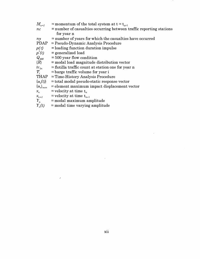
ny PDAP p(r) p
'(t) Qsoo {R} tcln T, THAP {u,(t)} {ue}max X��, xn+l Y,, Y,,(t)
= momentum of the total system at t = tn+l = number of casualties occurring between traffic reporting stations
for year n = number of years for which the casualties have occurred = Pseudo-Dynamic Analysis Procedure = loading function duration impulse = generalized load = 500 year flow condition = modal load magnitude distribution vector = flotilla traffic count at station one for year n = barge traffic volume for year i = Time-History Analysis Procedure = total modal pseudo-static response vector = element maximum impact displacement vector = velocity at time tn = velocity ·at time tn+l = modal maximum amplitude = modal time varying amplitude
Xll
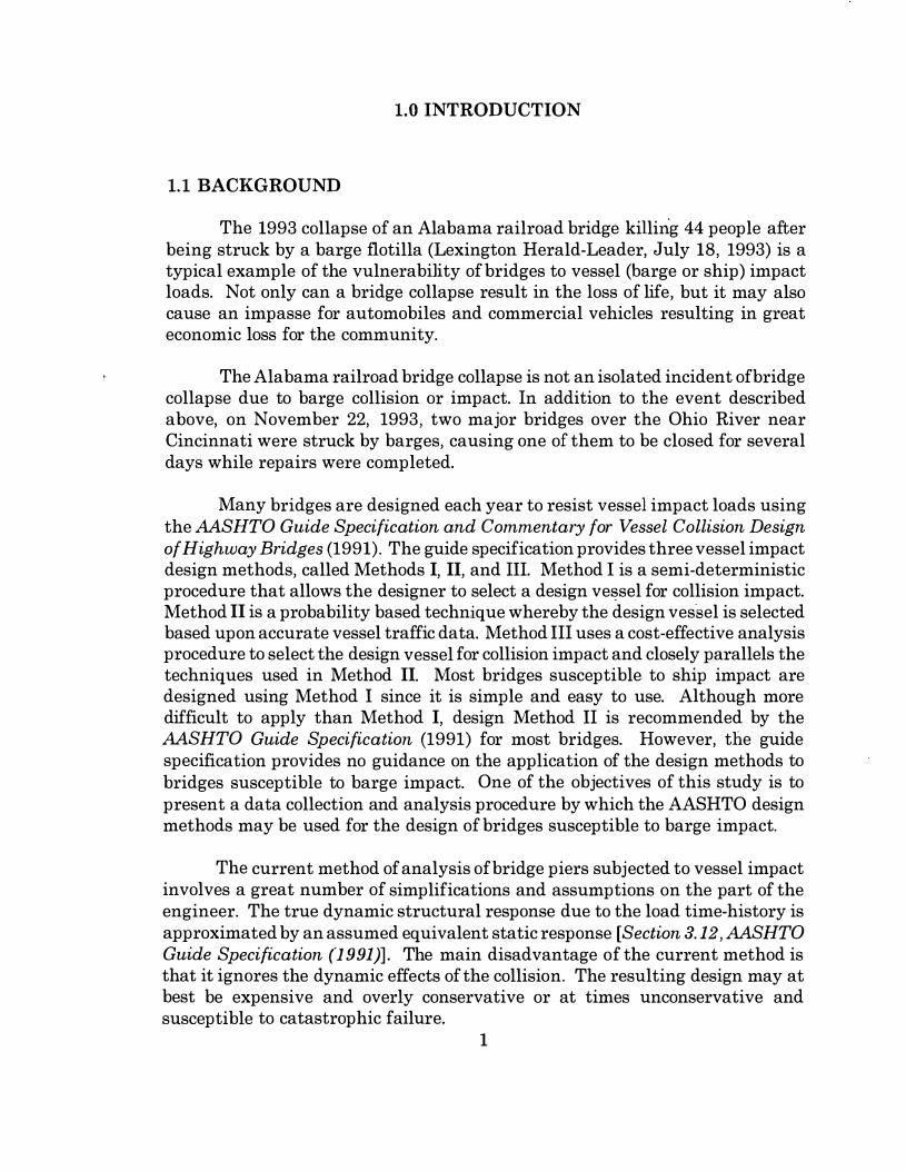
1.0 INTRODUCTION
1.1 BACKGROUND
The 1993 collapse of an Alabama railroad bridge killing 44 people after being struck by a barge flotilla (Lexington Herald-Leader, July 18, 1993) is a typical example of the vulnerability of bridges to vessel (barge or ship) impact loads. Not only can a bridge collapse result in the loss of life, but it may also cause an impasse for automobiles and commercial vehicles resulting in great economic loss for the community.
The Alabama railroad bridge collapse is not an isolated incident ofbridge collapse due to barge collision or impact. In addition to the event described above, on November 22, 1993, two major bridges over the Ohio River near Cincinnati were struck by barges, causing one of them to be closed for several days while repairs were completed.
Many bridges are designed each year to resist vessel impact loads using the AASHTO Guide Specification and Commentary for Vessel Collision Design of Highway Bridges (1991). The guide specification provides three vessel impact design methods, called Methods I, II, and III. Method I is a semi-deterministic procedure that allows the designer to select a design vessel for collision impact. Method II is a probability based technique whereby the design vessel is selected based upon accurate vessel traffic data. Method III uses a cost-effective analysis procedure to select the design vessel for collision impact and closely parallels the techniques used in Method II. Most bridges susceptible to ship impact are designed using Method I since it is simple and easy to use. Although more difficult to apply than Method I, design Method II is recommended by the AASHTO Guide Specification (1991) for most bridges. However, the guide specification provides no guidance on the application of the design methods to bridges susceptible to barge impact. One of the objectives of this study is to present a data collection and analysis procedure by which the AASHTO design methods may be used for the design of bridges susceptible to barge impact.
The current method of analysis of bridge piers subjected to vessel impact involves a great number of simplifications and assumptions on the part of the engineer. The true dynamic structural response due to the load time-history is approximated by an assumed equivalent static response [Section 3. 12, AASHTO Guide Specification (1991)]. The main disadvantage of the current method is that it ignores the dynamic effects of the collision. The resulting design may at best be expensive and overly conservative or at times unconservative and susceptible to catastrophic failure.
1

This study presents three design methodologies for modeling the dynamic interaction of the individual barges of the flotilla and the bridge during the collision event. A flotilla represents a train of barges tied together both length and width wise. Figure 1 .1 .1 shows a typical barge flotilla configuration. Each design method represents an increasing level of analysis complexity. The choice between the three design methods is based on the characteristics of the bridge (e.g. importance, regular or irregular, span lengths, etc.) as is currently done for seismic design of highway bridges.
2

(j) s 0
0:::
(J) 01 \._ 0
m
y
....: ----- ·)>
<-
.,.
Tuw Boot
Figure 1.1.1: Typical Barge Flotilla.
3

1.2 LITERATURE SURVEY
Very few publications relating to impact design of bridges are known to exist. The author located only three publications that related specifically to barge impact design of highway bridges. These publications, however, dealt with the development of the current AASHTO Guide Specification equivalent static design method. Since one of the goals of this study is to include dynamic effects these publications could not be used. Extensive existing literature was found that related to impact analysis of large structures and could be generally classified into four categories; missile impact with concrete structures, aircraft impact with concrete structures, vessel impact with offshore oil platforms, and train impact with rigid structures. These types of impact analysis will be investigated in the following sections.
1.2.1 Missile Impact
A great deal of work has been published on missile impact since it is related to national security. The major emphasis of this research is on finite element modeling of missile impact. An extensive literature search on this type of impact was conducted by Bangash, 1993. Missile impact finite element modeling is generally aimed at analyzing localized concrete impact effects, i.e., penetration of concrete structures. Missile impact applications can generally be classified as material non-linear dynamic finite analysis. These applications do not included the effects of soil continuum effects on the response of the structure. In addition, the computation and model mesh refinement required for application of these methods are of little practical benefit to the bridge designer faced with determining the overall response of a large and complicated structure.
1.2.2 Aircraft Impact
Aircraft impact analysis is generally aimed at nuclear reactor confinement building design since these types of structures must be able to resist accidental and terrorist aircraft impact. The nuclear regulatory agency has sponsored extensive research in this area and Bang ash, 1993 conducted an extensive literature search on the safety analysis of nuclear reactors to impact and explosion.
Nuclear reactor impact design research studies were found to be generally aimed at determining the non-linear concrete behavior with little or no consideration for soil structure interaction. As was the case with missile impact
4

analysis, the degree of continuum mesh refinement required is prohibitive when considering the large beam element bridge structure.
It should be noted that Riera, 1980, presented a model for determining aircraft impact loading functions that could be utilized for determining the impact loading function for a single barge impacting a rigid structure. Adaptation of this model resulted in the multiple barge loading functions.
1.2.3 Vessel Impact
Vessel impact design of offshore oil platforms is a problem similar to impact design of bridges susceptible to barge impact in that soil-structure interaction effects are particularly important. Pettersen, 1981, and Woisin, 1979, presented simplified soil-structure interaction analysis procedures; however, these procedures are strictly static analysis methods and do not allow for the consideration of distributed soil effects or the interaction between the individual pile elements.
1.2.4 Train Impact
Train impact is similar to barge impact in that the impact loading is the result of the interaction of multiple separate vehicles. The· British Rail Authority conducted crash tests of trains on rigid structures (Bangash, 1993) which were useful for verifying the general shape of the barge impact loading functions.
1.3 OBJECTIVES
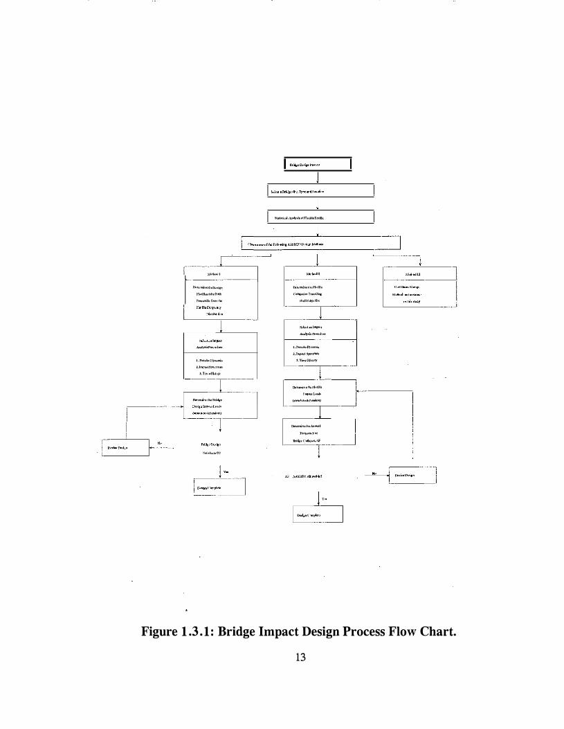
The objectives of this research are; 1) identification of the barge design flotillas, and their impact characteristics (impact velocity, impact elevation, etc.) that the inland waterways must be designed to resist (design flotillas), and 2) derivation of impact analysis procedures which account for the dynamic nature of the impact event. These two objectives encompass the complete process for impact analysis and design of waterway bridges. Figure 1.3 .1 graphically flow charts this bridge design process. In addition, Figure 1.3 .2 flow charts the steps necessary for the analysis of bridges susceptible to barge impact. The following sections outline in more detail the steps given in Figure 1.3.2.
5

1.3. 1 Design Flotillas
The first objective of this study is to identify the design flotillas and their characteristics necessary for design of bridges susceptible to barge impact. The design vessel can be determined using the AASHTO statistical design methods known as Methods I, II, or III. However, these methods are difficult to apply to barge traffic. Figure 1.3 .1 gives the AASHTO design procedure for bridges susceptible to vessel impact design in flow chart format. The following sections give the information and statistical analyses that are necessary to apply the AASHTO design methods to barge impact design following the flow chart of Figure 1.3.1 .
The barge traffic results for this study are based on statistical data obtained from the U.S. Coast Guard, the U.S. Army Corps of Engineers, and the American Waterways Operators, and are necessary to apply design Method II of the guide specification. Specifically, the data are needed to calculate:
o The probability of aberrancy; o The waterway elevation profiles; • The size and tonnages of the barges using the waterways; • The flotilla category distributions; • The future barge traffic projections; and • The average utilized cargo capacity.
1.3.1.1 Probability of Aberrancy
In order to calculate the probability of aberrancy on inland waterways in accordance with the AASHTO Guide Specification, long-term vessel casualty (accident) data are required. The U.S. Coast Guard, Marine Safety Evaluation Branch, Washington, D.C., maintains a database on vessel casualties for the waterways. The database contains casualty reports for all vessel types operating on the waterway system, including barge tows. In addition, the database gives the nature of the casualty, i.e. collision, grounding, etc. From this information the probability of aberrancy for particular segments of a waterway system are determined.
1.3. 1.2 Waterway and Impact Elevation
The elevations for the rivers are provided by the District Engineers of the U.S. Army Corps of Engineers. The river elevations for the normal pool, 2%, Q50, Q100, and Q500 flow conditions are needed for the rivers. As defined by the Army Corps of Engineers the normal pool is the river elevation above which
6

vegetation grows on the river banks, and the 2% flow river is the river elevation which is exceeded 2% of the time. The Q50, Q100, and Q500 flow are the river elevations that have a return period of 50, 100, and 500 years, respectively. The American Waterways Operators and the U.S. Coast Guard Captain of the Port can provide various records on barge draft depths, heights, etc. necessary for determining the impact elevation above the waterway elevation.
1.3.1.3 Barge Size and Tonnage
Barge tonnages and sizes are calculated using the information contained in the Waterborne Commerce of the United States database. This database is maintained by the U.S. Army Corps of Engineers' Waterborne Commerce Office in New Orleans, LA, and was released to the University of Kentucky under the Freedom of Information Act.
The database comes as a formatted ASCII (FASCII) file. Acomputer program was written to process the information and conduct a statistical analysis of the data in order to assign barge sizes and tonnages. Barge types are defined based on the U.S. Army Corps of Engineers barge length and width designation system.
1.3. 1.4 Flotilla Category
The application of the design methods in the AASHTO Guide Specification (1991) requires that the number of barges comprising the flotillas currently using the waterways be known. Therefore, the number of barges comprising the flotillas was determined based on the information contained in the 1992 Performance Monitoring System database provided by the U.S. Coast Guard Navigation Data Center, Washington, D.C. The information provided in the database is: A) the annual cumulative number of barges, based on the U.S. Army Corps of Engineers barge length and width designation system and B) the sizes and frequencies of the flotillas traveling on the waterways.
It should be noted that, although flotillas are not entirely comprised of one barge size or type, they are generally made up of mostly the same barge size and type. Nevertheless, there is still a very large variation in the flotillas using the inland waterway system. Therefore, a probability based approach was adopted to calculate the number of barges comprising a flotilla. Flotillas are then categorized based upon the primary barge type in the train. For example if a barge type is the primary barge in the flotilla then the flotilla category is designated as that barge type. A computer program was written to process the
7
database and calculate the number of barges to be assigned to the columns and rows of each flotilla category.
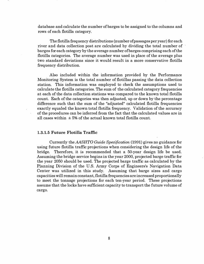
The flotilla frequency distributions (number of passages per year) for each river and data collection post are calculated by dividing the total number of barges for each category by the average number ofbarges comprising each of the flotilla categories. The average number was used in place of the average plus two standard deviations since it would result in a more conservative flotilla frequency distribution.
Also included within the information provided by the Performance Monitoring System is the total number of flotillas passing the data collection station. This information was employed to check the assumptions used to calculate the flotilla categories. The sum of the calculated category frequencies at each of the data collection stations was compared to the known total flotilla count. Each of the categories was then adjusted, up or down by the percentage difference such that the sum of the "adjusted" calculated flotilla frequencies exactly equaled the known total flotilla frequency. Validation of the accuracy of the procedures can be inferred from the fact that the calculated values are in all cases within ± 5% of the actual known total flotilla count.
1.3.1.5 Future Flotilla Traffic
Currently the AASHTO Guide Specification (1991) gives no guidance for using future flotilla traffic projections when considering the design life of the bridge. Therefore, it is recommended that a 50-year design life be used. Assuming the bridge service begins in the year 2000, projected barge traffic for the year 2050 should be used. The projected barge traffic as calculated by the Planning Division of the U.S. Army Corps of Engineers's Navigation Data Center was utilized in this study. Assuming that barge sizes and cargo capacities will remain constant, flotilla frequencies are increased proportionally to meet the tonnage projections for each ten-year period. These projections assume that the locks have sufficient capacity to transport the future volume of cargo.
8

1.3.1.6 Average Utilized Cargo Capacity
In addition to maintaining the Performance Monitoring System Database, the Navigation Data Center annually conducts a statistical analysis of the barge traffic on the U.S. waterway system. Among the results of the analysis are the average up bound cargo capacity, average downbound cargo capacity, and the average percentage change in total barge traffic at each of the data collection points on the U.S. waterways.
1.3.2 Analysis Procedures
The current barge impact design method, called the "equivalent static method" given in the AASHTO Guide Specification (1991) is a very simplistic design method that may not accurately predict the forces that a bridge may be subjected to during a collision event. However, this method is currently used to design even the largest and most vital bridges crossing inland waterways.
Three levels of analysis are proposed herein for barge impact design of bridges: A) Pseudo-Dynamic Analysis Procedure (PDAP), B) Impact Spectrum Analysis Procedure (ISAP), and C) Time-History Analysis Procedure (TRAP). Though the TRAP is obviously not a new method of general structural dynamic analysis, it is new in its application to barge impact design of bridges since no loading time-history has previously existed.
The proposed methods of analysis are analogous to the three levels that are currently used for seismic design of highway bridges: A) Surface Acceleration, B) Response Spectra, and C) Time-History. The level of analysis is dictated by the importance classification of the bridge, the dynamic load (or acceleration), the bridge is critical or non-critical classification of the bridge, and whether the bridge is regular or irregular construction of the bridge. The three proposed methods of analysis and the steps necessary for their development are described in the following sections.
1.3.2.1 Impact-Loading Functions
The first step in the derivation of the three analysis procedures is the determination of the barge flotilla loading functions. Based on past flotillabridge collision investigations, AASHTO suggests that only the barges in a single column of a multi-column flotilla be used in developing the impact loading (Section C3. 12 in AASHTO). This recommendation is based on the fact that barges in adjacent rows are lashed together with ropes that break during
9
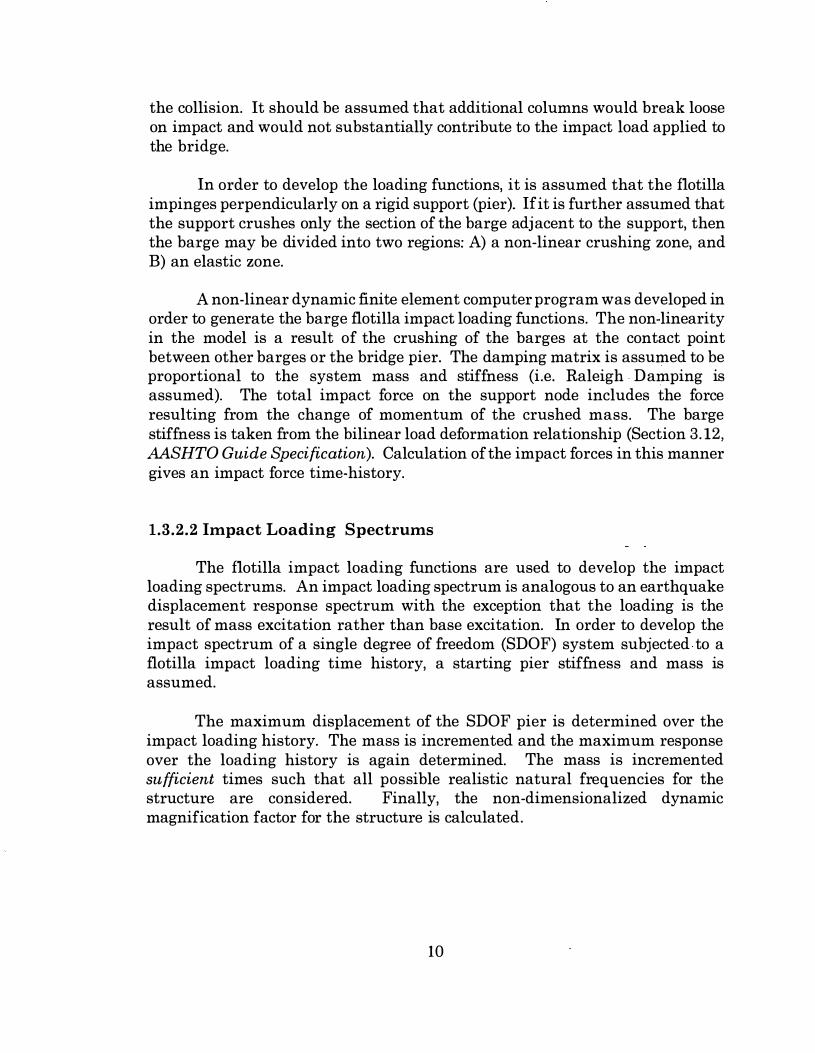
the collision. It should be assumed that additional columns would break loose on impact and would not substantially contribute to the impact load applied to the bridge.
In order to develop the loading functions, it is assumed that the flotilla impinges perpendicularly on a rigid support (pier). If it is further assumed that the support crushes only the section of the barge adjacent to the support, then the barge may be divided into two regions: A) a non-linear crushing zone, and B) an elastic zone.
A non-linear dynamic finite element computer program was developed in order to generate the barge flotilla impact loading functions. The non-linearity in the model is a result of the crushing of the barges at the contact point between other barges or the bridge pier. The damping matrix is assumed to be proportional to the system mass and stiffness (i.e. Raleigh . Damping is assumed). The total impact force on the support node includes the force resulting from the change of momentum of the crushed mass. The barge stiffness is taken from the bilinear load deformation relationship (Section 3. 12, AASHTO Guide Specification). Calculation of the impact forces in this manner gives an impact force time-history.
1.3.2.2 Impact Loading Spectrums
The flotilla impact loading functions are used to develop the impact loading spectrums. An impact loading spectrum is analogous to an earthquake displacement response spectrum with the exception that the loading is the result of mass excitation rather than base excitation. In order to develop the impact spectrum of a single degree of freedom (SDOF) system subjected to a flotilla impact loading time history, a starting pier stiffness and mass is assumed.
The maximum displacement of the SDOF pier is determined over the impact loading history. The mass is incremented and the maximum response over the loading history is again determined. The mass is incremented sufficient times such that all possible realistic natural frequencies for the structure are considered. Finally, the non-dimensionalized dynamic magnification factor for the structure is calculated.
10

1.3.2.3 Pseudo-Dynamic Analysis Procedure (PDAP)
In order to determine the approximate dynamic bridge response, the total dynamic response is resolved into the contribution of the lower modes and the higher modes. It can be shown that the response of higher frequency modes can be calculated by static analysis because their inertial effects are negligiblec Therefore, the response can be approximated by the contribution of the inertial response plus the static response.
For the simplified analysis procedure, only a single dynamic mode is considered to contribute significantly to the total dynamic response; therefore, the free vibration modal analysis is not required. Only a static analysis is needed where the structure is loaded with the maximum magnitude of the barge impact force time-history at the impact point plus the distributed inertial loading determined from the impact spectrum and the assumed mode shape. Generally, the distributed loading can be represented by a linear force distribution.
1.3.2.4 Impact Spectrum Analysis Procedure (ISAP)
The Impact Spectrum Analysis Procedure is similar to the preceding Pseudo-Dynamic Analysis Procedure. However, the dynamic response of the bridge is approximated by a combination of multiple inertial modes. In the analysis of bridges susceptible to barge impact, the higher mode shapes generally contribute significantly to the total response of the bridge during impact. This procedure allows for the determination of only the lower inertial mode shapes with the inclusion of the higher mode shape effects accomplished by neglecting their inertial contribution, and therefore including their pseudostatic response.
1.3.2.5 Time-History Analysis Procedure (THAP)
Though time-history analysis is not new by any means, time-history analysis of bridges susceptible to barge impact is made possible by utilizing the loading time-histories developed in this study. Generally, an impact timehistory analysis of a bridge would be required only for large expensive bridges. However, a time-history analysis of smaller bridges that have a high probability of barge impact may, in some cases, be warranted.
1 1

1.4 Research Significance
The research given in this study provides four distinct contributions to the development of an improved methodology ofbridge design for barge impact. When taken as a whole these four contributions provide analysis procedures that can be integrated into the current vessel impact design foundation given by the AASHTO Guide Specification for Vessel Impact Design of Highway Bridges. A description of these four categories along with the Section that they are presented in this study are given by the following:
1) Development of a statistical method by which barge traffic data can be used for impact design of inland waterway bridges (Section 2). The methods given may be utilized in conjunction with the current AASHTO Guide Specifications for design of bridges susceptible to maritime vessel impact. Though the methods given in this study were developed specifically using Kentucky barge traffic data, the methods are applicable to barge traffic anywhere in the United States or the World.
2) Derivation of multiple-barge impact time-histories using the single barge load-deformation curve provided in the AASHTO Guide Specification (Section 3). Currently, no impact time-histories are known to exist which would allow for rigorous analysis of and design of bridges susceptible to barge impact.
3) Derivation of design impact response curves. These design curves are developed by enveloping the impact response curves for the statistically significant barge groups (flotillas) identified in Section 2 (Section 3).
4) Development of three barge impact analysis procedures that may be used in place of the current AASHTO Equivalent Static analysis procedure (Sections 3, 4 and 5). The three methods developed allow for the inclusion ofthe effects of the dynamic interaction between the individual barges in the flotilla and the bridge. The current equivalent static method simplifies the impact problem to a simple static point load and ignores the dynamic nature of the barge impact problem.
The flow chart for the development of these four categories is given in Figure 1.3.3.
12
,------ - -i,- - :,�,:.::- __ _] '"�.,;,�,,.,,,,,'"
!loorill•ollh<l'"h
P""""'il• f•om li><
i ""''";"'"·�<1 ....
I.P .. I<o�>ll)o�rnl<
J.lme"'"""'"'"
,I.Tl,,_in,l"l>' ---1 -----
- - '�"'"'·"'"' ., :::.-- --]· · "''"'""'"'' -· -- 1-
,
""'"''""')'')
"'""'''� '"'>b'•l••>ll'ln"ii•T"I5o
M��_J-··.· '"�-mu ....... l .. llllo
,.,,.,.; .. T""'itlno
'"""""''·''''
,,l ... � .. , ...... _ _ -� ... .... � ....
I !'.u ... >l�""'"'"
· ::�::::::· - -�- -
-- ---, [}o�noj;�::·::· ��-'''""'""'"''"'""''' ----,-- ---"
w...ru"''"'AMwl I ,,,,_,, nri.r.•<"•Oi•l"�·ll' _j - � --
'
l l _,
Figure 1 .3 . 1 : Bridge Impact Design Process Flow Chart.
13

i I ' ---- --
Ne
'
---�- �J--Iu•�•ciAnul)�i'
of Wol<ll\11ytl<idg"
'
Timo-hi'""Y Anuly,iJ(/
�==�""'"'' .. J--� L.�,·:�R"-'P""-"" - -----� --1
(lmriLotSpcclnun)
'"
Figure 1 .3.2: Flow Chart for Impact Analysis of Waterway Bridges.
14

I Project Development Flow J y
I Statistical Design I Barge Flotillas Section 2
y
; f Method 2 Design Example I Appendix I
., J Flotilla Impact Loading Functions I Section 3
• I Flotilla Peak Impact Load Function I Section 3
f I Flotilla Impact Spectrwns I Section 3
., I Flotilla Impact Design Spectrums' Section 3
., I Impact Modal Response Equations I Section 4 y
Psuedo-Dynamic Analysis Procedure (PDAP)
General Design Equations Section 5
., Psuedo-Dynarnic Analysis Procedure (PDAP)
Step-by-Step Design Process
Section 5
y Psuedo-Dynamic Analysis Procedure (PDAP)
Design Examples and THAP Result Comparison Section 5
'f Impact Spectrum Analysis Procedure (ISAP)
General Design Equations
Appendix ill
'¥ Impact Spectrum Analysis Procedure (!SAP)
Step-by-Step Design Process
Appendix ill
y Impact Spectrum Analysis Procedure (ISAP)
Design Example and THAP Result Comparison
Section 5
Figure 1 .3.3: Project Development Flow Chart.
15

2.0 PROBABILITY BASED BARGE IMPACT DESIGN
2.1 INTRODUCTION
Currently, no inland waterway bridges are known to have been designed for barge impact using the AASHTO design methods due to the tremendous variation in flotilla sizes and barge types and sizes. There are presently two thousand known barge sizes and types in use; flotillas may contain an almost infinite variation ofthese barge sizes and types. This Section provides a method by which available barge and flotilla data may be used to apply the AASHTO design methods for barge impact on bridges in the navigable inland waterways of Kentucky, namely the Ohio, Tennessee, Cumberland, Green, and Kentucky Rivers. Although this study concentrated on barge traffic on Kentucky rivers, the methodologies presented are applicable to all navigable inland waterways in the United States and the World.
In 1993, a railroad bridge in Alabama collapsed after being struck by a barge flotilla during high water river flow conditions (Lexington Hearld-Leader, July 18, 1993). The bridge collapse resulted in the tragic loss of forty-four lives, and caused a major disruption in automobile and commercial vehicle traffic. As mentioned in Section 1, this Alabama bridge collapse is not an isolated event. On November 22, 1993, two major bridges over the Ohio River near Cincinnati were struck by barges, causing one of them to be closed for several days while repairs were completed.
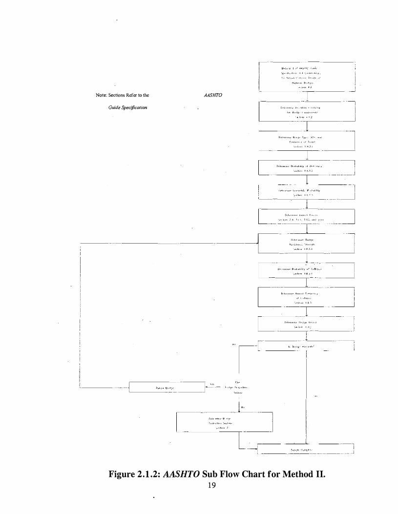
Many bridges are designed each year to resist vessel impact loads using the AASHTO Guide Specification and Commentary for Vessel Collision Design of Highway Bridges (1991). The guide specification provides three vessel impact design methods, called Methods I, II, and III. Figure 2 .1 .1 provides the AASHTO flow chart for design of highway bridges up to the point of determining which of Methods I, II, and III is to be used. Method I is a semi· deterministic procedure that allows the designer to select a design vessel for collision impact. Method II is a probability based technique whereby the design vessel is selected based upon accurate vessel traffic data. Method III uses a cost-effective analysis procedure to select the design vessel for collision impact and closely parallels the techniques used in Method II. Method III will not be discussed in this study.
Most bridges are designed using an assumed design flotilla that may or may not be the critical flotilla determined using either design Methods I or II. Method I is easier to use than Method II; however, design Method II is recommended by theAASHTO Guide Specification (1991) for most bridges. The flow chart for design of a highway bridge is provided in Figure 2.1.2. The guide specification provides no guidance on the application of any of the design
16

methods to bridges susceptible to barge impact since it focuses mostly on ship impact design.
The data included in this study are in accordance with the AASHTO Guide Specification (1991). The results generated are based on statistical data obtained from the U.S. Coast Guard, the U.S. Army Corps of Engineers, and the American Waterways Operators. Specifically, the data necessary to apply design Method II of the guide specification are the following: 1) barge size and capacities, 2) the number of barges in a flotilla column and row, 3) river elevations, 4) flotilla transit velocity, and 5) probabilities of aberrancy. Currently, the AASHTO Guide Specification (1991) provides a simple method for calculating the equivalent static barge impact force on a bridge element. The formulas are based on impact tests conducted on individual European barges (Meir, and Dornberg, 1980). However, this is of concern since the tests are conducted on single barges at low velocities and not on multi-barge flotillas traveling at high velocities as found on the rivers of Kentucky.
This Section presents a method for identifying the inland waterway design flotillas using the AASHTO Guide Specification statistical design methods, called Methods I, II, and III. No bridge is known to have been designed using Method II, even though this method is recommended by AASHTO. This is due to the tremendous variation in the barge sizes, and types comprising the inland flotillas. In a later Section, the design flotillas will be utilized to develop three impact analysis procedures for true dynamic design of bridges susceptible to impact by the design flotillas. True dynamic design produces distributed member loads that are a result of the inertial effects ofthe impact load time-history. The current AASHTO equivalent static method uses a single static point load to simulate the dynamic interaction ofthe flotilla and bridge.
17

Note: Sections refer to the AASHTO
Figure 2 .1 .1 : AASHTO Design Procedure Flow Chart.
18
Note: Sections Refer to the AASHTO
Guide Specification
... -- ! __ }-"'-
,--- · I " ''" '"'""' , , . ,,., :•---"'" I H .. ,,,,.,, B , .. ,,,_,
···--- I I r
I [•et.-. ..... .- ••• ,. ...... - ._,,.,,. I' ,_,. .. .... , •• < '""""'""' . ' _ : ·:·: i_" " __ __j
,------- ;, ___ _ L n"'" """ B'"''" '"" ''"'""'" ' "' ,,_,._,
.......... ' " ' '
- ·----------,-�:'"'"'"'" '''"'"''""'' "' '"'"'' "" ' L_ .. ____
·�
·-
"
"
"
'
,
" , " [ [t,.,,.,,..,," ""'"'' ' ""'· '
"' ' "- ' ' ' - 1 1 ;: . ..... , , , , -- -----,- -- --' C- ---,L__''''''' n .. ,.,. ..... ... " � .. ,.; "'"' ' """
'"'"
' ' � ' - '
'"' '' "''"'''" ' "' , .,,,,,, .... '·"''""' ' " '
- � __ _ j
I _ __j
J
i ! - -
L ... , 1 --- _L __
---- ]
�'''""'""" ""';,,,. v •• ,.,,._., '-"' --""" - - ---- -
"'" .,.,,,,_, ..
--, ---- ------ __ j
Figure 2.1 .2: AASHTO Sub Flow Chart for Method II. 19

2.2 DATA COLLECTION
The data included in this report are in accordance with the AASHTO Guide Specification and Commentary for Vessel Collision Design of Highway Bridges. The results generated are based on statistical data obtained from the U.S. Coast Guard, the U.S. Army Corps of Engineers, and the American Waterways Operators, and are necessary for applying design Method II of the guide specification. Specifically, the data are needed to calculate:
• the probability of aberrancy, • the size and tonnages of the barges using the waterways, • the flotilla category distributions, • the number of barges in the flotilla column and row, and • the waterway elevation profiles.
In order to calculate the probability of aberrancy on Kentucky waterways in accordance with the AASHTO Guide Specification, long-term vessel casualty (accident) data are required. The U.S. Coast Guard, Marine Safety Evaluation Branch, Washington, D .C., has maintained a database on vessel casualties for the past 11 years for Kentucky waterways. The database contains casualty reports for all vessel types operating on the waterway system, including barge tows. In addition, the database gives the nature of the casualty, i.e. collision, grounding, ramming, etc.
A data query was conducted by the U.S. Coast Guard computer specialists for the University of Kentucky under the Freedom of Information Act. From this information, the probability of aberrancy for particular segments of the Kentucky waterway system was determined. This is shown diagrammatically in Figure 2.2.1 .
The information necessary to calculate the flotilla category distributions and the number of barges in the flotilla columns or rows was provided by the U.S. Coast Guard Navigation Data Center, Washington, D.C., from the Performance Monitoring System database. The purpose of the database is to track the efficiency of movement of cargo by barge along the U.S. inland waterway system. Data collection points for the database are located at the locks on the waterway system.
The information provided in the database is the annual cumulative number ofbarges categorized by the U.S. Army Corps of Engineers classification system and the sizes and frequencies of the flotillas traveling on the waterways. From the information provided in the database, the flotilla frequency distribution by category, and the number of barges to be assigned to the flotilla column and row are calculated. This is illustrated in Figures 2.2.2 and 2.2.3.
20

The database was not released to the University of Kentucky because of the size and complexity of the data files. All data queries were conducted by the U.S. Army Corps of Engineers' computer specialists with the results sent to the University of Kentucky on computer disks; generally requiring five to six MBytes of storage. Computer programs were then written to process the query results and conduct a statistical analysis on the data.
In addition to maintaining the Performance Monitoring System Database, the N avigation Data Center annually conducts a statistical analysis of the barge traffic on the U.S. waterway system. Among the results of the analysis are the average upbound cargo capacity, average downbound cargo capacity, and the average percentage change in total barge traffic at each of the data collection points on the U.S. waterways. Average upbound and downbound capacities, and changes in barge traffic are collected for Kentucky waterways for the most recent years of 1992 and 1993.
Barge type tonnages and sizes are calculated using the information contained in the Waterborne Commerce of the United States database. This database is maintained by the U.S. Army Corps of Engineers' Waterborne Commerce Office in New Orleans, LA, and was released to the University of Kentucky under the Freedom of Information Act. The database requires approximately 7.2 MBytes of computer storage and comes as a formatted ASCII (FASCII) file. A computer program was written to process and conduct a statistical analysis of the data in order to assign barge sizes and tonnages to the 24 barge types. The information flow is shown in Figure 2.2.4.
The elevations for the rivers of Kentucky are provided by the U.S. Army Corps District Engineers. Figure 2.2.5 lists the three district engineers who provided information for all of Kentucky's waterways. It should be noted that the Nashville District Office acted in cooperation with the Tennessee Valley Authority. The river elevations for the normal pool, 2%, Q50, Q100, and Q500 flow conditions are sought for all of Kentucky's navigable rivers. As defined by the Army Corps of Engineers, the normal pool is the river elevation above which vegetation grows on the river banks, and the 2% flow river is the river elevation which is exceeded 2% of the time. The Q50, Q100, and Q500 flow are the river elevations that have a return period of 50, 100, and 500 years, respectively. However, for some sections of the Kentucky and Cumberland Rivers, complete data records are not maintained and the information was not available from any known source.
The American Waterways Operators and the U.S. Coast Guard Captain of the Port, Louisville, KY, provided various records on barge transit speeds, typical flotilla sizes, barge draft depths, etc. This is illustrated in Figures 2.2.6 and 2.2. 7.
21
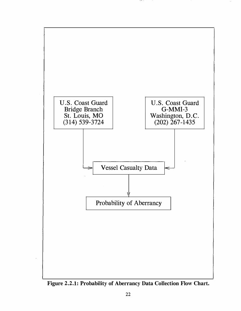
U . S . Coast Guard U . S . Coast Guard Bridge Branch G-MMI-3 St. Louis, MO Washington, D . C . (3 14) 539-3724 (202) 267-1435
-
L;.. Vessel Casualty Data. �
Probability of Aberrancy
Figure 2.2.1: Probability of Aberrancy Data Collection Flow Chart.
22

U . S . Army Corps of Engineers Navigation Data Center
Washington, D . C . (703) 355-3061
I
Performance Monitoring System -
II
Total Barge Distribution Data Barge Traffic Growth Rate
Upbound/Downbound Cargo Capacities
Figure 2.2.2: Total Barge Distribution Data Collection Flow Chart.
23

Army Corps of Engineers Navigation Data Center
Washington, D . C . (703)-355-306 1
II/
Performance Monitoring System
II/
Flotilla Dimensions Distribution Data
Figure 2 .2.3: Flotilla Dimensions Data Collection Flow Chart.
24
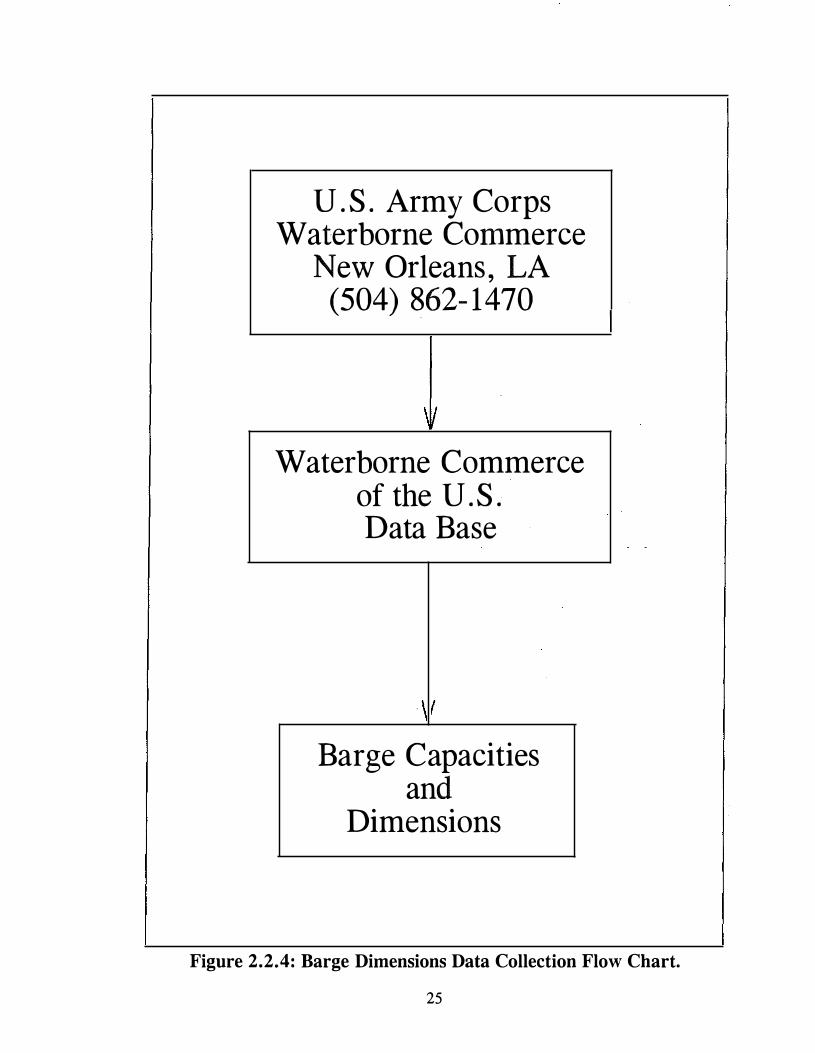
U . S . Army Corps Waterborne Commerce
New Orleans , LA (504) 862- 1470
I I
Waterborne Commerce of the U . S . Data Base
. \ I
Barge Capacities and
Dimensions
Figure 2.2.4: Barge Dimensions Data Collection Flow Chart.
25
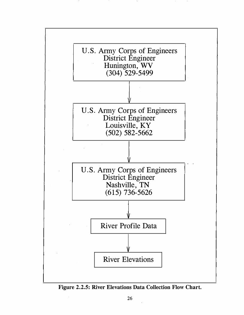
U.S . Army Corps of Engineers District Engineer Hunington, WV (304) 529-5499
It
U.S . Army Corps of Engineers District Engineer Louisville, KY (502) 582-5662
U.S . Army Corps of Engineers District Engineer
Nashville , TN (6 1 5) 736-5626
I
River Profile Data
River Elevations
Figure 2.2.5: River Elevations Data Collection Flow Chart.
26

American Waterways Operators Inland Waterways
(703) 841 -9300
-
I I
General Information
Figure 2.2.6: General Information Data Collection Flow Chart.
27

U . S . Coast Guard Louisville, KY (502) 582-5 194
\II
Captain of the Port
Barge Transit Velocities Maximum Barge Draft Depth
. Figure 2.2.7: Barge Transit Velocities Data Collection Flow Chart.
28
2.3 BARGE SIZES AND CAP A CITIES
In order to apply Method II of the AASHTO Guide Specification, the barge sizes and displacement tonnages comprising the flotillas currently using the waterways of Kentucky must be determined. The 24 barge types defined in this study are based on the U.S. Army Corps of Engineers barge length and width designation system and are given in Table 2.3.1 (see Figure 2.3.1 for the definition of barge length and width). The sizes and tonnages associated with the 24 barge types are based on the information contained in the Waterborne Transportation Lines of the United States database, 1993. The database contains sizes and tonnages of every barge registered to operate in the U.S. A computer program was written to process the database and calculate the sizes and tonnages to be assigned to the barges comprising a flotilla category. The computer calculations are based on the following assumptions:
1. The variation of the barge sizes and tonnages within a category can be represented by a normal distribution.
2. The barges using the waterways of Kentucky do not exceed a loaded draft of 15.2-ft. Figure 2.3.2 shows the concept of "loaded draft."
The draft cutoff of 15.2-ft was based on information from the U.S. Coast Guard that barges with a draft in excess of 12-ft do not typically operate on Kentucky waterways. The 15.2-ft value was used to include some barges in the database that could conceivably operate during high water conditions. This will lead to reasonably conservative results.
3. The minimums of the following values are used:
• The maximum sizes, and tonnages encountered for a category within the database.
• The average sizes and tonnages plus two standard deviations calculated for a category.
Since the variation of the barge sizes and tonnages within a category can be represented by a normal distribution, use of the average plus two standard deviations assures that the barge sizes and tonnages assigned to a category have only a 2.25% chance of being exceeded. In case the maximum value within a category is less than the average plus two standard deviations, then the maximum value is used. Since the database contains all barges operating within Kentucky waterways, if the maximum value is
29

used, there is a 0% chance that the sizes and tonnages will be exceeded.
4. Only barges typically operating on the Mississippi River System and the Gulf Coast Intercostal Waterway are used in the calculations.
5. The barge self weight could be linearly interpolated from the relationship:
li: lhf ----------(2.1)
,_knit
d1nff t_11-rJii
Figures 2.3.2 and 2.3.3 illustrate typical barge length and width distributions for flotilla categories BB and HD, respectively.
Barges using the Kentucky waterways may not always be fully loaded when operating on the waterway system. Table 2.3.4 gives the average percentage of cargo capacity for the up bound and downbound barges at each of the data collection points on the Kentucky rivers. The cargo capacities are calculated by the Navigation Data Center in its annual statistical analysis of the barge traffic on the U.S. waterway system.
30
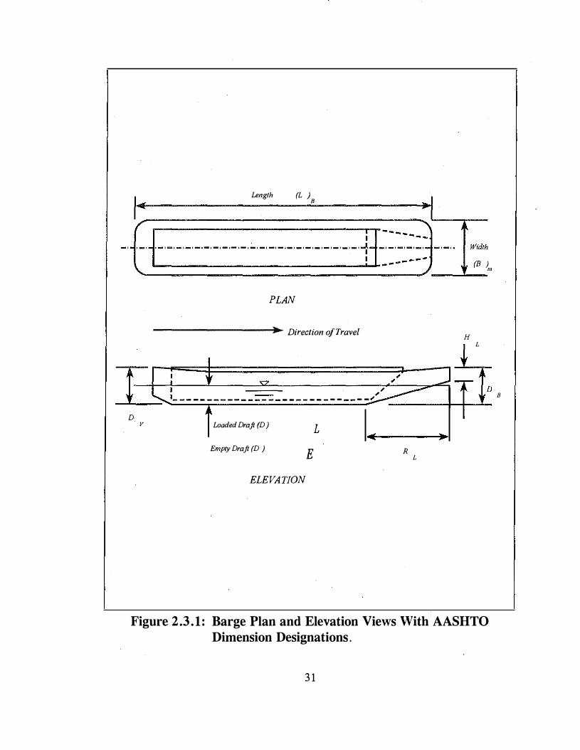
I Length (L )8 . I I ·��� -{+- - - - - - - - - - - - - - - - - - - - - 1E�::J--L-- · - · · �:�:,
PLAN
----------:!� Direction of Travel H � L
H-:1,... _ _ ==_=_= _ _ �=_=_= __ =_=_=_ �=-=_= __ =_=_ = __ =_= __ =_=_= _ _ =,=,:_---=_;=,�����j+-+--,--1-D
B
D v Loaded Draft (D) L
Empty Draft (D ) R E L
ELEVATION
Figure 2.3 .1 : Barge Plan and Elevation Views With AASHTO Dimension Designations .
3 1

ClJ t :::J (j (j
Cl "--() "--ClJ
-C) E :::J
<
ClJ t :::J (j (j
Cl "--() "--ClJ
-C) E :::J
<
Figure 2.3.2:
, ,_,.,,
·�, ,1'
.i, l r '
�,'II
_'(it '
1i 'r '
lr.lr.h)
8c•rJ
''UU
-li'l '
,_'(·Y!
,,
S'cll'r)l;' Width (ti)
Typical Barge Length and Width Distribution for Flotilla Category BB.
32

Table 2.3.1: Barge Length and Width Designations.
Dimension Designation Range*
A less than 100 feet
B 100 to 174 feet
Length c 175 to 194 feet
D 195 to 199 feet
E 200 to 259 feet
F 260 to 289 feet
G 290 to 300 feet
H greater than 300 feet .
A less than 26 feet Width B 26 to 34 feet
c 35 to 54 feet
D greater than 54 feet
* Note: 1 foot = 0.3048 meters
33
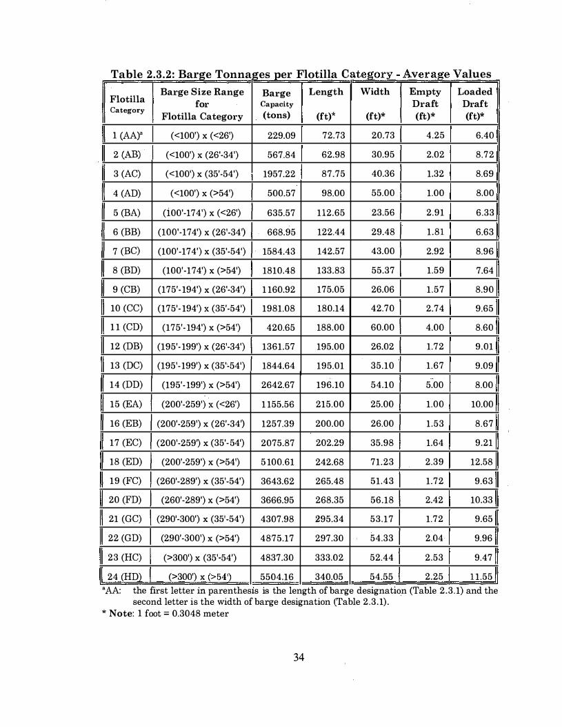
Table 2.3.2: Barge Tonnages per F oti a 1 11 c ategory - A verage V I a ues
Barge Size Range Barge Length Width Empty Loaded Flotilla for Capacity Draft Draft Category
Flotilla Category (tons) (ft)* (ft)* (ft)* (ft)*
1 (AA)" (<100') X (<26') 229.09 72.73 20.73 4.25 6.40
2 (AB) (<100') X (26'-34') 567.84 62.98 30.95 2.02 8.72
3 (AC) (<100') X (35'-54') 1957.22 87.75 40.36 1.32 8.69
4 (AD) (<100') X (>54') 500.57 98.00 55.00 1.00 8.00
5 (BA) (100'-174') X (<26') 635.57 112.65 23.56 2.91 6.33
6 (BB) (100'-17 4') X (26'-34 � . 668.95 122.44 29.48 1.81 6.63
7 (BC) (100'-174') X (35'-54') 1584.43 142.57 43.00 2.92 8.96
8 (BD) (100'-174') X (>54') 1810.48 133.83 55.37 1.59 7.64
9 (CB) (175'-194') X (26'-34') 1 160.92 175.05 26.06 1.57 8.90
10 (CC) (175'-194') X (35'-54') 1981.08 180.14 42.70 2.74 9.65
1 1 (CD) (175'-194') X (>54') 420.65 188.00 60.00 4.00 8.60
12 (DB) (195'-199') X (26'-34') 1361.57 195.00 26.02 1.72 9.01
13 (DC) (195'-199') X (35'-54') 1844.64 195.01 35.10 1.67 9.09
14 (DD) (195'-199') X (>54') 2642.67 196.10 54.10 5.00 8.00
15 (EA) (200'-259') X (<26') 1 155.56 215.00 25.00 1.00 10.00
16 (EB) (200'-259') X (26'-34� 1257.39 200.00 26.00 1.53 8.67
17 (EC) (200'-259') X (35'-54') 2075.87 202.29 35.98 1.64 9.21
18 (ED) (200'-259') X (>54') 5 100.61 242.68 71.23 2.39 12.58
19 (FC) (260'-289') X (35'-54') 3643.62 265.48 51.43 1.72 9.63
20 (FD) (260'-289') X (>54') 3666.95 268.35 56.18 2.42 10.33
21 (GC) (290'-300') X (35'-54') 4307.98 295.34 53.17 1.72 9.65
22 (GD) (2.90'-300') X (>54') 4875.17 297.30 54.33 2.04 9.96
23 (HC) (>300') X (35'-54') 4837.30 333.02 52.44 2.53 9.47
24 (HD) (>300') X (>54') 5504.16 340.05 54.55 2.25 11.55 'AA: the first letter m parenthesis IS the length of barge designatiOn (Table 2.3.1) and the
second letter is the width of barge designation (Table 2.3.1). * Note: 1 foot = 0.3048 meter
34
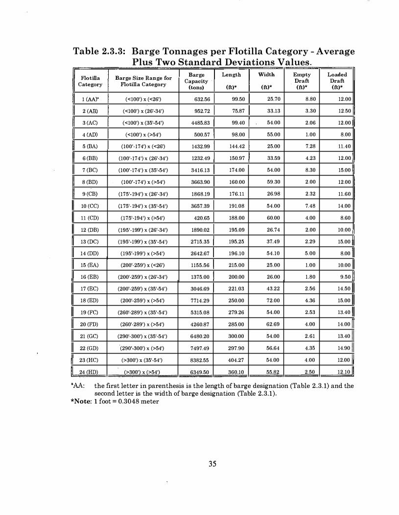
Table 2.3.3: Barge Tonnages per Flotilla Category - Average Plus Two Standard Deviations Values
Flotilla Barge Size Range for Barge Length Width Empty Loaded
Category Flotil la Category Capacity Draft Draft
(tons) (ft)* (ft)* (ft)* (ft)*
1 (AA)" (<100') X (<26') 632.56 99.50 25.70 8.80 12.00
2 (AB) (<100') X (26'-34') 952.72 75.87 33.13 3.30 12.50
3 (AC) (<100') X (35'-54') 4485.83 99.40 54.00 2.06 12.00
4 (AD) (<100') X (>54') 500.57 98.00 55.00 1.00 8.00
5 (BA) (100'-174') X (<26') 1432.99 144.42 25.00 7.28 ll.40
6 (BB) (100'-174') X (26'-34') 1232.49 150.97 33.59 4.23 12.00
7 (BC) (100'-174') X (35'-54') 3416.13 174.00 54.00 8.30 15.00
8 (BD) (100'-17 4') X (>54') 3663.90 160.00 59.30 2.00 12.00
9 (CB) (175'-194') X (26'-34') 1868.19 176.ll 26.98 2.32 11.60
10 (CC) (I 75'- 194') X (35'·54') 3657.39 191.08 54.00 7.48 14.00
ll (CD) (175'-194') X (>54') 420.65 188.00 60.00 4.00 8.60
12 (DB) (195'-199') X (26'·34') 1890.02 195.09 26.74 2.00 10.00
13 (DC) (195'-199') X (35'·54') 2715.35 195.25 37.49 2.29 15.00
14 (DD) (195'-199') X (>54') 2642.67 196.10 54.10 5.00 8.00
15 (EA) (200'-259') X (<26') 1155.56 215.00 25.00 1.00 10.00
16 (EB) (200'-259') X (26'-34') 1375.00 200.00 26.00 1.80 9.50
17 (EC) (200'-259') X (35'-54') 3046.69 221.03 43.22 2.56 14.50
18 (ED) (200'-259') X (>54') 7714.29 250.00 72.00 4.36 15.00
19 (FC) (260'-289') X (35'-54') 5315.08 279.26 54.00 2.53 13.40
20 (FD) (260'-289') X (>54') 4260.87 285.00 62.69 4.00 14.00
21 (GC) (290'-300') X (35'-54') 6480.20 300.00 54.00 2.61 13.40
22 (GD) (290'-300') X (>54') 7497.49 297.90 56.64 4.35 14.90
23 (HC) (>300') X (35'-54') 8382.55 404.27 54.00 4.00 12.00
24 (HD) (>300') X (>54') 6349.50 360.10 55.82 2.50 12.10
'AA: the first letter in parenthesis is the length of barge designation (Table 2.3.1) and the second letter is the width of barge designation (Table 2.3.1).
*Note: 1 foot = 0.3048 meter
35
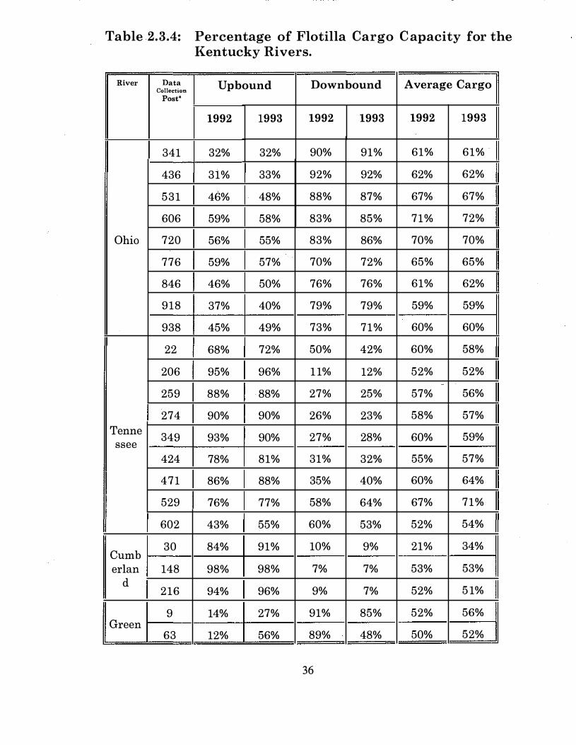
Table 2.3.4: Percentage of Flotilla Cargo Capacity for the Kentucky Rivers.
River Data Up bound Down bound Average Cargo Collection Post"
1992 1993 1992 1993 1992 1993
341 32% 32% 90% 91% 61% 61% .
436 31% 33% 92% 92% 62% 62%
531 46% 48% 88% 87% 67% 67%
606 59% 58% 83% 85% 71% 72%
Ohio 720 56% 55% 83% 86% 70% 70%
776 59% 57% 70% 72% 65% 65%
846 46% 50% 76% 76% 61% 62%
918 37% 40% 79% 79% 59% 59%
938 45% 49% 73% 71% 60% 60%
22 68% 72% 50% 42% 60% 58%
206 95% 96% 11% 12% 52% 52%
259 88% 88% 27% 25% 57% 56%
274 90% 90% 26% 23% 58% 57% Tenne 349 93% 90% 27% 28% 60% 59% ssee
424 78% 81% 31% 32% 55% 57%
471 86% 88% 35% 40% 60% 64%
529 76% 77% 58% 64% 67% 71%
602 43% 55% 60% 53% 52% 54%
Cumb 30 84% 91% 10% 9% 21% 34%
erlan 148 98% 98% 7% 7% 53% 53% d
216 94% 96% 9% 7% 52% 51%
9 14% 27% 91% 85% 52% 56% Green
63 12% 56% 89% 48% 50% 52%
36

2.4 FLOTILLA CATEGORIES
The application of Method II of the AASHTO Guide Specification (1991) requires that the number of barges comprising the flotillas currently using the waterways be known. Therefore, the numbers of barges comprising flotillas are determined based on the information contained in the 1992 Performance Monitoring System database provided by the U.S. Coast Guard Navigation Data Center, Washington, D.C. The purpose of the database is to track the efficiency of barge cargo movement along the U.S. inland waterway system. The information provided in the database is: 1) the annual cumulative number of barges, based on the U.S. Army Corps of Engineers barge length and width designation system presented previously in Table 2.3. 1 ; and 2) the sizes and frequencies of the flotillas traveling on the waterways.
As was mentioned in section 2.2, the database was not released to the University of Kentucky because of the size and complexity of the data files. Again, all data queries were conducted by the U.S. Army Corps of Engineers'. The results requiring five to six MBytes of storage were sent to the University of Kentucky. Fortran computer codes were then written to process the query results and conduct a statistical analysis on the data.
It should be noted that, although flotillas are not entirely comprised of one barge size or type, they are generally made up of mostly the same barge size and type. Nevertheless, there is still a very large variation in the flotillas using the Kentucky waterway system. Therefore, a probability based approach was adopted to calculate the number of barges comprising a flotilla. Flotillas are then categorized based upon the primary barge type in the flotilla. Therefore, the idealized flotilla category's designation is the same as the primary barge type comprising the flotilla. For example, if barge type CC is the primary barge in the flotilla then the flotilla category is designated as CC. This idealization process is shown in Figure 2.4.1.
The computer program written to process the database and calculate the number of barges to be assigned to the columns and rows of each flotilla category was based on the following assumptions:
1 . The variation of the number ofbarges comprising the columns and rows of a flotilla within a flotilla category could be represented by a normal distribution.
2. Since the flotilla width seemingly varies in regular increments, the number of barges in a row is decided first.
37
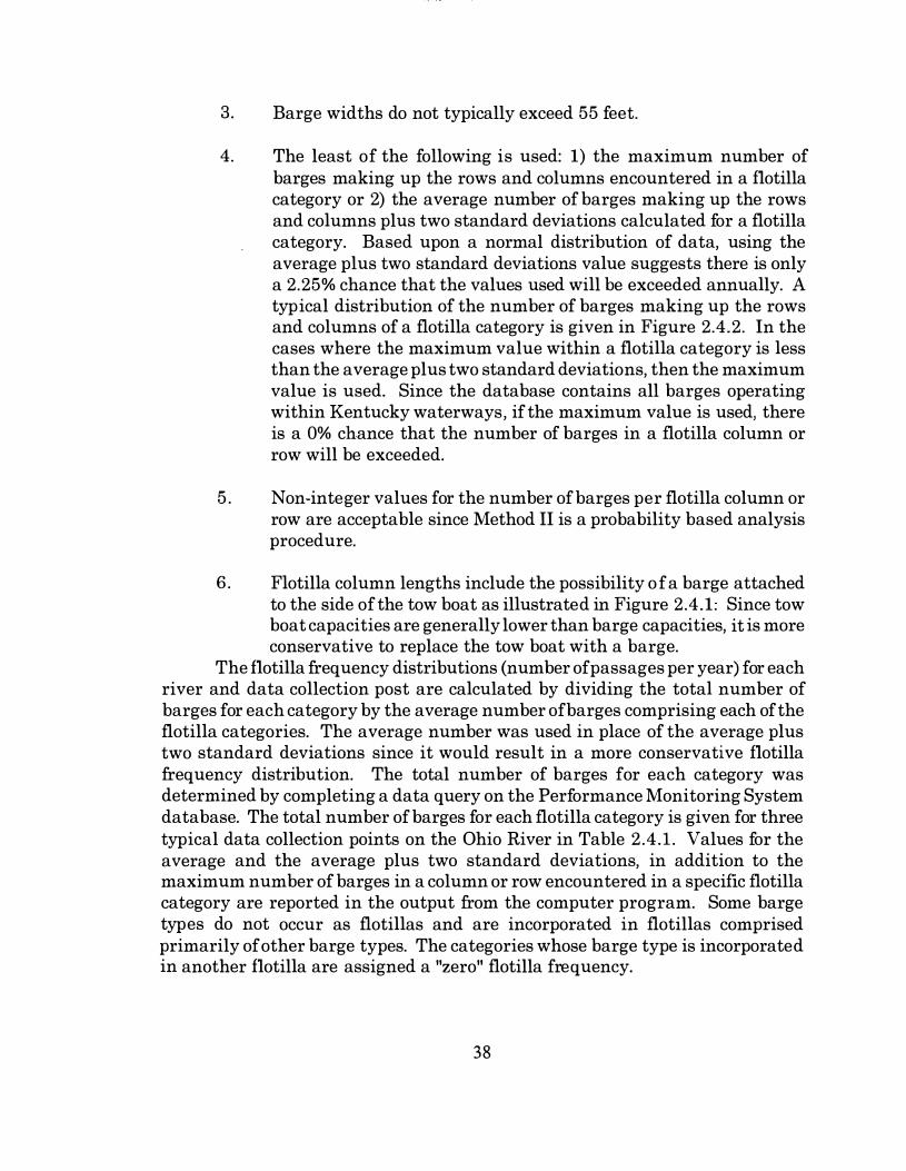
3. Barge widths do not typically exceed 55 feet.
4. The least of the following is used: 1) the maximum number of barges making up the rows and columns encountered in a flotilla category or 2) the average number of barges making up the rows and columns plus two standard deviations calculated for a flotilla category. Based upon a normal distribution of data, using the average plus two standard deviations value suggests there is only a 2.25% chance that the values used will be exceeded annually. A typical distribution of the number of barges making up the rows and columns of a flotilla category is given in Figure 2.4.2. In the cases where the maximum value within a flotilla category is less than the average plus two standard deviations, then the maximum value is used. Since the database contains all barges operating within Kentucky waterways, if the maximum value is used, there is a 0% chance that the number of barges in a flotilla column or row will be exceeded.
5 . Non-integer values for the number of barges per flotilla column or row are acceptable since Method II is a probability based analysis procedure.
6. Flotilla column lengths include the possibility of a barge attached to the side of the tow boat as illustrated in Figure 2.4.1. Since tow boat capacities are generally lower than barge capacities, it is more conservative to replace the tow boat with a barge.
The flotilla frequency distributions (number of passages per year) for each river and data collection post are calculated by dividing the total number of barges for each category by the average number ofbarges comprising each of the flotilla categories. The average number was used in place of the average plus two standard deviations since it would result in a more conservative flotilla frequency distribution. The total number of barges for each category was determined by completing a data query on the Performance Monitoring System database. The total number of barges for each flotilla category is given for three typical data collection points on the Ohio River in Table 2.4.1. Values for the average and the average plus two standard deviations, in addition to the maximum number of barges in a column or row encountered in a specific flotilla category are reported in the output from the computer program. Some barge types do not occur as flotillas and are incorporated in flotillas comprised primarily of other barge types. The categories whose barge type is incorporated in another flotilla are assigned a "zero" flotilla frequency.
38

Also included within the information provided by the Performance Monitoring System is the total number of flotillas passing the data collection station. This information was employed to check the assumptions used to calculate the flotilla categories. The sum of the calculated category frequencies at each of the data collection stations was compared to the known total flotilla count. The totals compared generally with less than 1% difference with the largest error for any data station on a Kentucky waterway being less than 5% difference. Each of the categories was then adjusted up or down by the percentage difference as illustrated in Table 2.4.2, such that the sum of the "adjusted" calculated flotilla frequencies exactly equaled the known total flotilla frequency.
39

Actual Flotilla Idealized Flotilla
Figure 2 .4.1 : Flotilla Idealization Example.
40
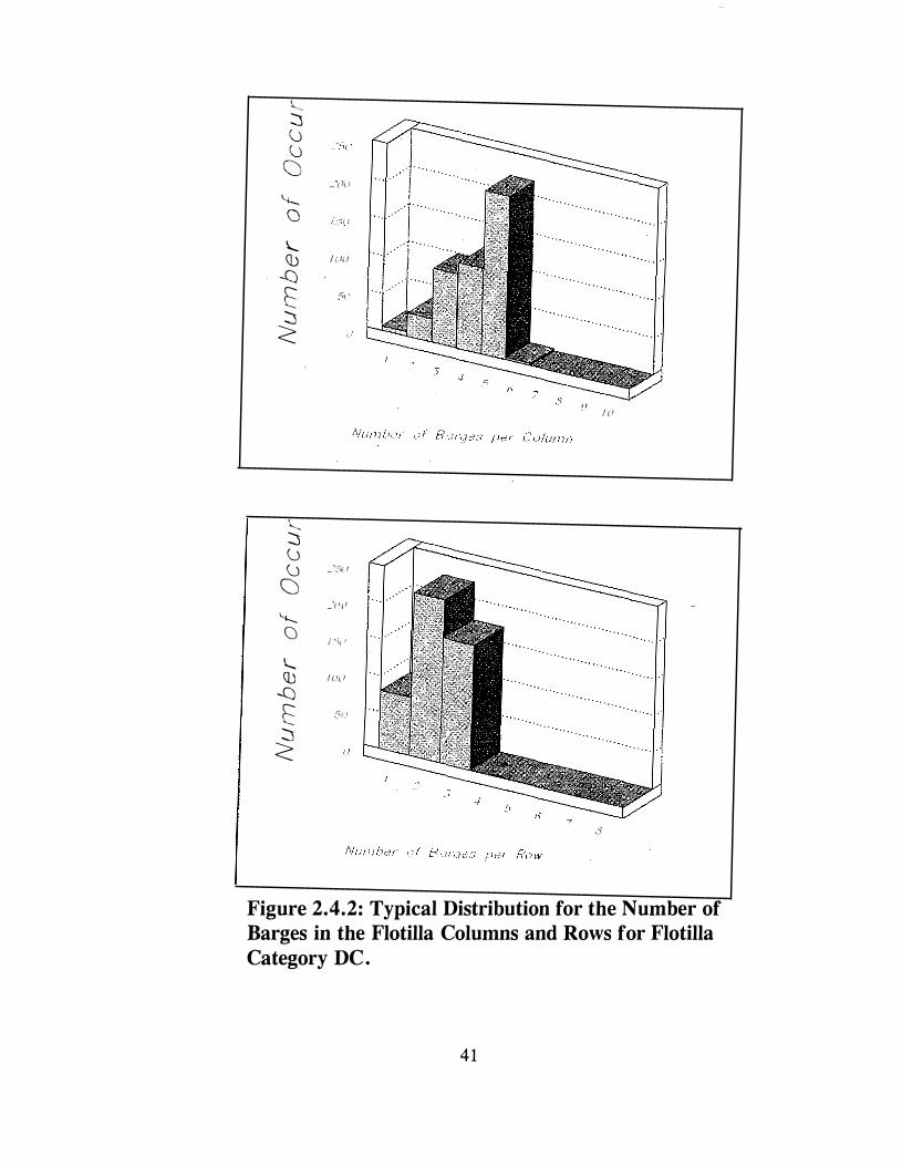
\..__ :::J \j \j
C) _'! h i
"-----C) i:."'<i I
\..__ (Jj I !_li_l
-C) l ."-r '
:::J <
/ I I
\..__ :::J \j \j -'-"ii_ l
C) _'( If!
"-----C)
/ ·'i,
\..__ (Jj I /)1_ I
-C) l ::;r_'
:::J <
;3
Figure 2.4.2: Typical Distribution for the Number of Barges in the Flotilla Columns and Rows for Flotilla Category DC.
41

Table 2.4.l:Total Barge Distribution Data for the Ohio River Miles 279-436.
Flotilla Barge Size Range Number of Barges
for Category
Flotilla Category* Mile 279* Mile 341* Mile 436*
1 (AA)" (<100') X (<2G') 43 5 18
2 (AB) (<100') X (2G'-34') 79 29 30
3 (AC) (<100') X (35'-54') 24 7 1
4 (AD) (<100') X (>54') 25 0 0
5 (BA) (100'-174') X (<2G') 13 0 0
G (BB) (100'-17 4') X (26'-34') 127 45 43
7 (BC) (100'-174') X (35'-54') 1,303 1,114 1 ,170
8 (BD) (lQQ'-174') X (>54') 2 1 0
9 (CB) (175'- 194') X (2G'-34') 1,994 33 70
10 (CC) (175'-194? X (35'-54') GOG G42 571
11 (CD) (175'-194') X (>54') 114 G8 11
12 (DB) (195'-199') X (26'-34') 5,384 228 233
13 (DC) (195'-199') X (35'-54') 28,232 54,694 51,269
14 (DD) (195'-199') X (>54') 101 52 1 1
1 5 (EA) (200'-259') X (<2G? 1 0 0
16 (EB) (200'-259') X (26'-34') 52 1 4
17 (EC) (200'-259') X (35'-54') 3,807 4,415 4,822
18 (ED) (200'-259') X (>54') 31 6 15
19 (FC) (260'-289') X (35'-54') 106 127 70
20 (FD) (260'-289') X (>54') 0 9 1
21 (GC) (290'-300') X (35'-54') 2,195 3,1 1 1 2,628
22 (GD) (290'-300') X (>54') 8 5 15
23 (HC) (>300') X (35'-54') 36 170 30
24 (HD) (>300') X (>54') 134 264 61
TOTAL 44 417 65,026 61,073
'AA: the first letter in parenthesis is the length of barge designation and the second letter is the width of barge designation (Table 2.3.1).
* Note: 1 foot = 0.3048 meter, 1 mile = 1.6093 kilometers. " distance in miles: below Pittsburgh for the Ohio River.
42
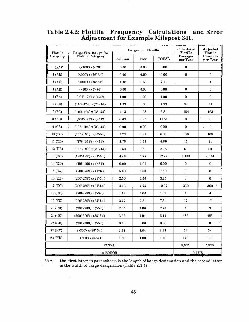
Table 2.4.2: Flotilla Frequency Calculations and Error Adjustment for Example Milepost 341.
Barges per Flotilla Calculated Adjusted Flotilla Barge Size Range for Flotilla Flotilla
Category Flotilla Category column TOTAL
Passages Passages row per Year per Year
1 (AA)" (<100') X (<26') 0.00 0.00 0.00 0 0
2 (AB) (<100') X (26'-34') 0.00 0.00 0.00 0 0
3 (AC) (<100') X (35'-54') 4.38 1.63 7.11 1 1
4 (AD) (<100') X (>54') 0.00 0.00 0.00 0 0
5 (BA) (100'-174') X (<26') 1.00 1.00 1.00 0 0
6 (BB) (100'-17 4') X (26'-34') 1.33 1.00 1.33 34 34
7 (BC) (100'- 17 4� X (35'-54� 4.13 1.65 6.81 164 163
8 (BD) (100'-174') X (>54') 6.63 1.75 11 .59 0 0
9 (CB) (175'-194') X (26'-34') 0.00 0.00 0.00 0 0
10 (CC) (175'-194') X (35'-54') 3.23 1.87 6.04 106 106
1 1 (CD) (175'·194') X (>54') 3.75 1.25 4.69 15 14
12 (DB) (195'-199') X (26'-34') 2.50 1.50 3.75 6 1 60
13 (DC) (195'-199') X (35'-54') 4.46 2.75 12.27 4,458 4,454
14 (DD) (195'-199') X (>54') 0.00 0.00 0.00 0 0
15 (EA) (200'-259') X (<26') 5.00 1.50 7.50 0 0
16 (EB) (200'-259') X (26'-34') 2.50 1.50 3.75 0 0
17 (EC) (200'-259') X (35'-54') 4.46 2.75 12.27 360 360
18 (ED) (200'-259') X (>54') 1.67 1.00 1.67 4 4
19 (FC) (260'-289') X (35'-54') 3.27 2.31 7.54 17 17
20 (FD) (260'-289') X (>54') 2.75 1.00 2.75 3 3
21 (GC) (290'-300') X (35'-54') 3.32 1.94 6.44 483 483
22 (GD) (290'-300') X (>54') 0.00 0.00 0.00 0 0
23 (HC) (>300') X (35'-54') 1.91 1.64 3.13 54 54
24 (HD) (>300') X (>54') 1.50 1.00 1.50 176 176
TOTAL 5,935 5,930
% ERROR 0.0775
'AA: the first letter in parenthesis is the length of barge designation and the second letter is the width of barge designation (Table 2.3.1)
43

Table 2.4.3: Ohio River Total Barge Traffic Growth Rates.
Mile Percent Changea
1991-1992 1 992-1993
341 1 7% 0%
436 -2% 3%
531 -2% 6%
606 -6% 3%
720 -8% 3%
776 -8% 4%
846 -8% 1% ...
918 -6% -2%
938 -5% 2%
' Percent change in barge traffic is calculated by the U.S. Army Corps of Engineers as:
T - T , . '
T ' . '
where T, is the barge traffic report for year i.
44
2.5 FUTURE BARGE TRAFFIC
Currently, the AASHTO Guide Specification gives no guidance for using future barge traffic projections when considering the design life of the bridge. Therefore, it is recommended that a 50-year design life be used. Assuming the bridge service begins in the year 2000, projected barge traffic for the year 2050 should be used. Table 2.4.3 gives the actual recorded barge traffic growth rates for 1991 and 1992 for all data collection points on the Ohio River. Table 2.5.1 gives the projected barge traffic for a typical data collection post on the Ohio River as calculated by the Planning Division of the U.S. Army Corps of Engineers's Navigation Data Center. Assuming that barge sizes and cargo capacities will remain constant, flotilla frequencies are increased proportionally to meet the tonnage projections for each ten year period. These projections assume that the locks have sufficient capacity to transport the future volume of cargo. Complete percentage tables are presented elsewhere (Whitney, et.al. 1994).
45

Table 2.5.1: Flotilla Frequency Projections for Ohio River, Milepost 341.
Flotilla Fiotilla Frequency (Number of Passages Per Year) Category 1992 2000 2010 2020 2030 2040 2050
1 (AA)a 0 0 0 0 0 0 0
2 (AB) 0 0 . 0 0 0 0 0
3 (AC) 1 1 2 2 2 2 2
4 (AD) 0 0 0 0 0 0 0
5 (BA) 0 0 0 . 0 0 0 0
6 (BB) 34 47 54 6 1 68 76 82
7 (BC) 163 226 261 294 328 365 392
8 (BD) 0 0 0 0 0 0 0
9 (CB) 0 0 0 0 0 0 0
10 (CC) 106 147 170 192 213 238 255
1 1 (CD) 14 19 22 25 28 31 34
12 (DB) 60 83 96 108 121 134 144
13 (DC) 4,454 6,189 7,133 8,047 8,963 9,982 10,719
14 (DD) 0 0 0 0 0 0 - 0
15 (EA) 0 0 0 0 0 0 0
16 (EB) 0 0 0 0 0 0 0
17 (EC) 360 500 577 650 724 807 866
18 (ED) 4 6 6 7 8 9 10
19 (FC) 17 24 27 31 34 38 41
20 (FD) 3 4 5 5 6 7 7
21 (GC) 483 671 774 873 972 1,082 1,162
22 (GD) 0 0 0 0 0 0 0
23 (HC) 54 75 86 98 109 121 130
24 (HD) 176 245 282 318 354 394 424
aAA The first letter in parentheses refers to the length of barge designation as presented in Table 2. 3. 1, and the second letter in parentheses refers to the width of barge designation as presented in Table 2.3.1.
46
2.6 RIVER ELEVATIONS
The AASHTO Guide Specification and Commentary for Vessel Collision Design of Highway Bridges appears to require that the barge impact loads be applied at the river 2% flow elevation. As determined from daily river flow data, the 2% flow elevation is the elevation the river exceeds just 2% of the time. The normal pool, 2% flow, Q50, Q100, and Q500 elevations are reported at regular intervals along most of the navigable inland waterways in Kentucky, as exemplified in Tables 2.6.1 for the Ohio River with complete tables for all Kentucky waterways presented elsewhere (Whitney, et.al. 1994) . The river elevations are provided by the U.S. Army Corps of Engineers offices in Louisville, KY, Nashville, TN, and Huntington, WV. The river elevations for the normal pool, 2%, Q50, Q100 and Q500 flow conditions are sought for all of the rivers in Kentucky that supported barge traffic. However, as mentioned previously, for some sections of the Kentucky and Cumberland Rivers, complete data records are not maintained and the information was not available from any known source.
47
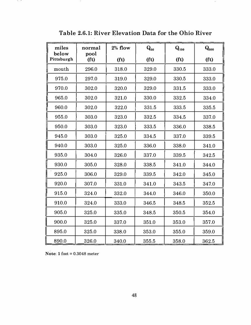
Table 2.6. 1: River Elevation Data for the Ohio River
miles normal 2% flow Q.o QlOO Q600 below pool
Pittsburgh (ft) (ft) (ft) (ft) (ft)
mouth 296.0 318.0 329.0 330.5 333.0
975.0 297.0 319.0 329.0 330.5 333.0
970.0 302.0 320.0 329.0 331.5 333.0
965.0 302.0 321.0 330.0 332.5 334.0
960.0 302.0 322.0 331.5 333.5 335.5
955.0 303.0 323.0 332.5 334.5 337.0
950.0 303.0 323.0 333.5 336.0 338.5
945.0 303.0 325.0 334.5 337.0 339.5
940.0 303.0 325.0 336.0 338.0 341.0
935.0 304.0 326.0 337.0 339.5 342.5
930.0 305.0 328.0 338.5 341.0 344.0
925.0 306.0 329.0 339.5 342.0 345.0
920.0 307.0 331.0 341.0 343.5 347.0
915.0 324.0 332.0 344.0 346.0 350.0
910.0 324.0 333.0 346.5 348.5 352.5
905.0 325.0 335.0 348.5 350.5 354.0
900.0 325.0 337.0 351.0 353.0 357.0
895.0 325.0 338.0 353.0 355.0 359.0
890.0 326.0 340.0 355.5 358.0 362.5
Note: 1 foot = 0.3048 meter
48

Table 2.6.1 (cont.): River Elevation Data for the Ohio River.
miles normal 2% flow Q50 QlOO Q500 below pool
Pittsburgh (ft) (ft) (ft) (ft) (ft)
885.0 327.0 341.0 357.5 359.5 364.0
880.0 327.0 343.0 359.0 361.5 366.0
875.0 327.0 344.0 360.5 363.0 368.0
870.0 328.0 346.0 362.0 364.5 369.0
865.0 329.0 347.0 364.0 366.0 371.0
860.0 330.0 349.0 365.0 367.0 372.0
855.0 330.0 351.0 366.0 368.5 373.0
850.0 331.0 352.0 366.5 369.0 373.5
845.0 342.0 353.0 367.5 369.5 374.0
840.0 343.0 355.0 368.5 370.5 374.0
835.0 343.0 356.0 369.0 371.0 375.0
830.0 344.0 358.0 369.5 371.5 375.5
825.0 345.0 359.0 371.0 372.5 376.5
820.0 345.0 361.0 371.5 373.0 377.0
815.0 345.0 362.0 372.5 374.0 378.0
810.0 346.0 364.0 373.5 375.0 378.0
805.0 346.0 365.0 374.5 376.5 378.5
800.0 347.0 367.0 375.5 377.0 379.0
795.0 347.0 369.0 376.0 378.0 380.0
Note: 1 foot = 0.3048 meter
49
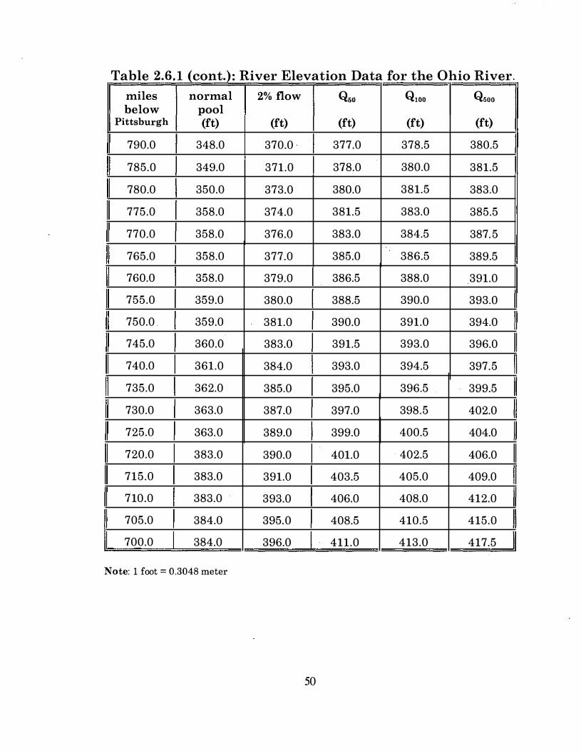
Table 2 6 1 (cont )· River Elevation Data for the Ohio River . . . .
miles normal 2% flow Q.o QlOO Q500 below pool
Pittsburgh (ft) (ft) (ft) (ft) (ft)
790.0 348.0 370.0 377.0 378.5 380.5
785.0 349.0 371.0 378.0 380.0 381.5
780.0 350.0 373.0 380.0 381.5 383.0
775.0 358.0 374.0 381.5 383.0 385.5
770.0 358.0 376.0 383.0 384.5 387.5
765.0 358.0 377.0 385.0 386.5 389.5
760.0 358.0 379.0 386.5 388.0 391.0
755.0 359.0 380.0 388.5 390.0 393.0
750.0 359.0 381.0 390.0 391.0 394.0
745.0 360.0 383.0 391.5 393.0 396.0
740.0 361.0 384.0 393.0 394.5 397.5
735.0 362.0 385.0 395.0 396.5 . 399.5
730.0 363.0 387.0 397.0 398.5 402.0
725.0 363.0 389.0 399.0 400.5 404.0
720.0 383.0 390.0 401.0 402.5 406.0
715.0 383.0 391.0 403.5 405.0 409.0
710.0 383.0 393.0 406.0 408.0 412.0
705.0 384.0 395.0 408.5 410.5 415.0
700.0 384.0 396.0 411.0 413.0 417.5
Note: 1 foot = 0.3048 meter
50
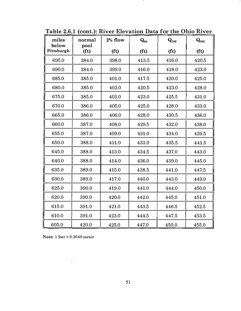
Table 2 6 1 (cont )· River Elevation Data for the Ohio River . . . .
miles normal 2% flow Q60 QlOO Q500 below . pool
Pittsburgh (ft) (ft) (ft) (ft) (ft)
695.0 384.0 398.0 413.5 416.0 420.5
690.0 384.0 399.0 416.0 418.0 423.0
685.0 385.0 401.0 417.5 420.0 425.0
680.0 385.0 402.0 420.5 423.0 428.0
675.0 385.0 403.0 423.0 425.5 431.0
670.0 386.0 405.0 425.0 428.0 433.0
665.0 386.0 406.0 428.0 430.5 436.0
660.0 387.0 408.0 429.5 432.0 438.0
655.0 387.0 409.0 431.0 434.0 439.5
650.0 388.0 411.0 433.0 435.5 441.5
645.0 388.0 413.0 434.5 437.0 443.0
640.0 388.0 414.0 436.0 439.0 445.0
635.0 389.0 415.0 438.5 441.0 447.5
630.0 389.0 417.0 440.0 443.0 449.0
625.0 390.0 419.0 441.0 444.0 450.0
620.0 390.0 420.0 442.0 445.0 451.0
615.0 391.0 421.0 443.5 446.5 452.5
610.0 391.0 423.0 444.5 447.5 453.5
605.0 420.0 425.0 447.0 450.0 455.0
Note: 1 foot = 0.3048 meter
5 1
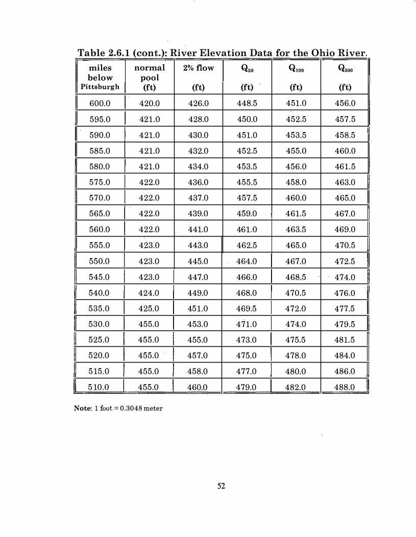
Table 2.6. 1 (cont.)· River Elevation Data for the Ohio River . .
miles normal 2% flow Qso QlOO Q500 below pool
Pittsburgh (ft) (ft) (ft) (ft) (ft)
600.0 420.0 426.0 448.5 451.0 456.0
595.0 421.0 428.0 450.0 452.5 457.5
590.0 421.0 430.0 451.0 453.5 458.5
585.0 421.0 432.0 452.5 455.0 460.0
580.0 421.0 434.0 453.5 456.0 461.5
575.0 422.0 436.0 455.5 458.0 463.0
570.0 422.0 437.0 457.5 460.0 465.0
565.0 422.0 439.0 459.0 461.5 467.0
560.0 422.0 441.0 461.0 463.5 469.0
555.0 423.0 443.0 462.5 465.0 470.5
550.0 423.0 445.0 464.0 467.0 472.5
545.0 423.0 447.0 466.0 468.5 474.0
540.0 424.0 449.0 468.0 470.5 476.0
535.0 425.0 451.0 469.5 472.0 477.5
530.0 455.0 453.0 471.0 474.0 479.5
525.0 455.0 455.0 473.0 475.5 481.5
520.0 455.0 457.0 475.0 478.0 484.0
515.0 455.0 458.0 477.0 480.0 486.0
5 10.0 455.0 460.0 479.0 482.0 488.0
Note: 1 foot = 0.3048 meter
52

Table 2.6 1 (cont ): River Elevation Data for the Ohio River . . .
miles normal 2% flow Q60 Q, •• Q, •• below pool
Pittsburgh (ft) (ft) (ft) (ft) (ft)
505.0 456.0 462.0 481.0 484.0 490.5
500.0 456.0 464.0 483.0 486.0 492.0
495.0 456.0 466.0 485.5 488.5 495.0
490.0 456.0 468.0 487.5 491.0 497.0
485.0 457.0 470.0 489.5 492.5 499.0
480.0 457.0 472.0 491.0 494.5 501.0
475.0 457.0 473.0 493.0 496.0 502.5
470.0 458.0 475.0 495.5 498.5 505.5
465.0 458.0 477.0 497.5 500.5 507.5
460.0 459.0 479.0 499.0 502.5 509.5
455.0 460.0 481.0 500.5 503.5 510.5
450.0 461.0 482.0 501.5 504.5 511.5
445.0 462.0 484.0 502.5 505.0 512.5
440.0 463.0 486.0 503.5 506.5 513.5
435.0 485.0 487.0 504.5 507.5 514.0
430.0 485.0 489.0 506.0 509.0 elevations
425.0 485.0 491.0 507.5 511.0 are not
420.0 486.0 493.0 509.0 512.5 available
415.0 486.0 494.0 510.5 514.0
Note: 1 foot = 0.3048 meter
53
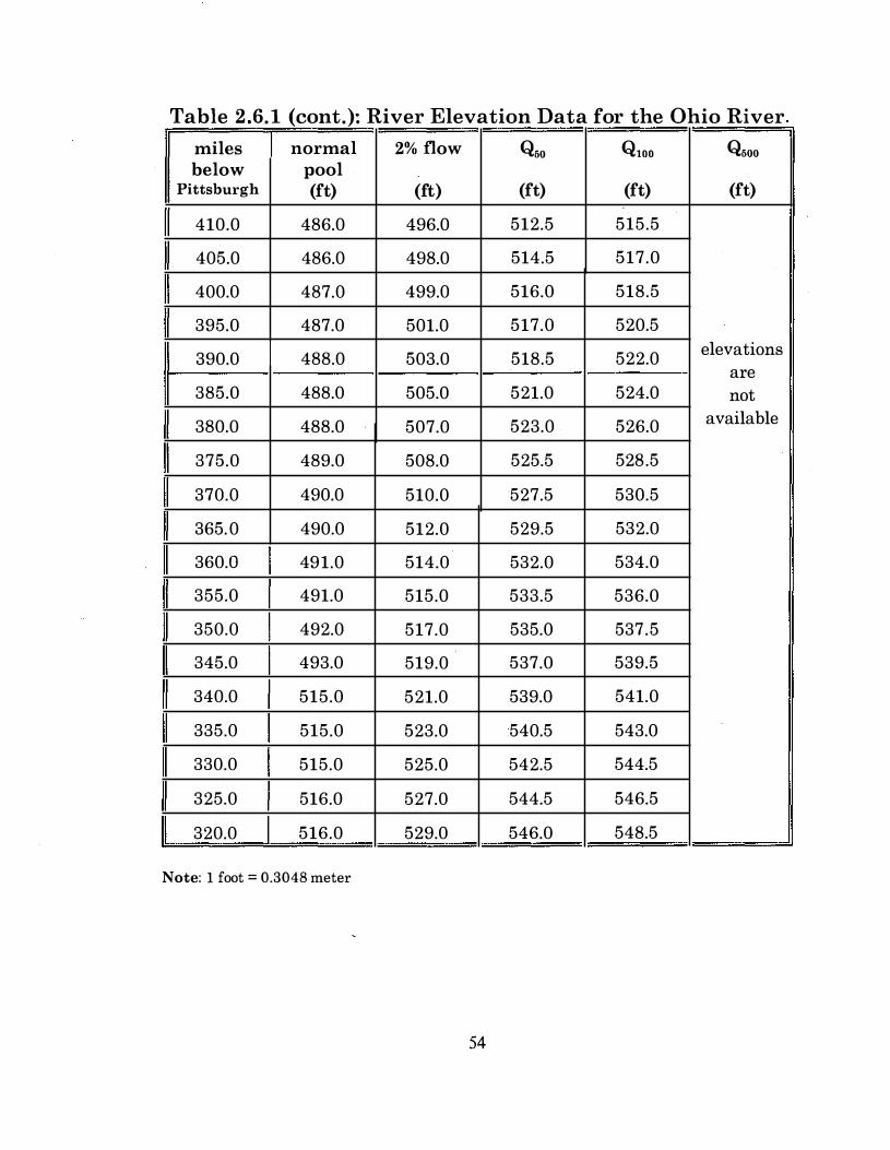
Table 2 6 1 (cont )· River Elevation Data for the Ohio River . . . .
miles normal 2% flow Q •• QlOO Q ••• below pool
Pittsburgh (ft) (ft) (ft) (ft) (ft)
410.0 486.0 496.0 512.5 515.5
405.0 486.0 498.0 514.5 517.0
400.0 487.0 499.0 516.0 518.5
395.0 487.0 501.0 517.0 520.5
390.0 488.0 503.0 518.5 522.0 elevations are
385.0 488.0 505.0 521.0 524.0 not
380.0 488.0 507.0 523.0 526.0 available
375.0 489.0 508.0 525.5 528.5
370.0 490.0 510.0 527.5 530.5
365.0 490.0 512.0 529.5 532.0
360.0 491.0 514.0 532.0 534.0
355.0 491.0 515.0 533.5 536.0
350.0 492.0 517.0 535.0 537.5
345.0 493.0 519.0 537.0 539.5
340.0 515.0 521.0 539.0 541.0
335.0 515.0 523.0 540.5 543.0
330.0 515.0 525.0 542.5 544.5
325.0 516.0 527.0 544.5 546.5
320.0 516.0 529.0 546.0 548.5
Note: 1 foot = 0. 3048 meter
54

2. 7 FLOTILLA VELOCITY
Flotilla velocity is the speed that a flotilla can achieve if the river velocity is zero (total velocity minus the river velocity). The maximum velocity is dependent on many factors including the power of the tow boat, the number and size of the individual barges in the flotilla, and the size of the load in each barge. Since there are so many variations possible for these factors, a logical approach to determining the flotilla velocity at a particular bridge site is to physically measure the flotilla total velocity and subtract the river velocity.
A second approach is to use a conservative upper bound velocity that would represent the maximum attainable speed for a fully loaded (or nearly fully loaded) flotilla traveling under ideal conditions. Table 2 .7 .1 gives the maximum attainable speeds for fully loaded flotillas under ideal conditions as determined by a survey of the U.S. Coast Guard and the barge operators. Presently, there is no known recorded barge traffic on the Kentucky River. Therefore, the minimum value of 5 mph in the table is warranted for future barge traffic.
Though the upper bound approach leads to conservative results, it may be too conservative when the structure is located on a section of a river where the flotilla must reduce speed in order to maintain control. For these cases, it may be desirable to survey the U.S. Coast Guard to determine the usual speeds at the bridge location or to physically measure the total velocity and deduct the river velocity at the time of measurement.
55
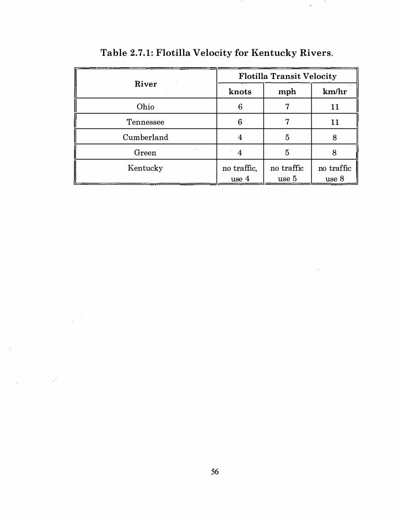
Table 2.7. 1 : Flotilla Velocity for Kentucky Rivers.
River Flotilla Transit Velocity
knots mph kmlhr
Ohio 6 7 11
Tennessee 6 7 11
Cumberland 4 5 8
Green 4 5 8
Kentucky no traffic, no traffic no traffic use 4 use 5 use 8
56

2.8 PROBABILITY OF ABERRANCY
The likelihood that a flotilla will be out of control (aberrant) must be determined in order to calculate the probability that a flotilla will collide with a bridge. Therefore, calculating the probability of aberrancy (PA) on Kentucky waterways in accordance with the AASHTO Guide Specification (1991) required long-term vessel casualty (accident) data. The U.S. Coast Guard, Marine Safety Evaluation Branch, Washington, D.C., has maintained a database on vessel casualties since 1983 for Kentucky waterways. The database contains casualty reports for all vessel types operating on the waterway system, including barge tows.
The casualty reports are stored as a database and contain the location, cause, type of vessel, and type of casualty. The types of casualties include: collisions with bridges, collisions with other vessels, collisions with docks, collisions with locks, and collisions with the river banks. Each barge within an aberrant flotilla is treated as a separate casualty record or event. For example, if a flotilla were comprised of 15 barges, of which eight are damaged, there would be eight separate casualty records in the database. However, since the impacts from the individual barges are applied simultaneously as a unit (i.e., a flotilla), only one of the casualties should be used in calculating the probability of aberrancy. In addition, if more than one flotilla is involved in a collision each flotilla should be treated as a separate event.
The AASHTO Guide Specification (1991) recommends that all types of barge casualties should be used to calculate the probability of aberrancy. Current ongoing research at the University of Kentucky questions whether grounding and ramming should be used in the calculations. However, since their inclusion leads to more conservative results, it is recommended that almost all types of barge casualties be incorporated in the aberrancy calculations. The only exceptions are casualties which are not the result of flotilla aberrancy, such as grounding on or collisions with submerged, unmarked obstacles.
In order to calculate the probability of aberrancy for a navigable waterway, the total number of flotilla casualties for a year is divided by the total number of flotillas traveling the river for that year. However, the waterways of Kentucky are occasionally hundreds of miles long and the flotilla operating conditions may change dramatically along the river. Therefore, the probability of aberrancy is calculated and given for ranges of the navigable rivers of Kentucky.
The ranges of the rivers are selected so that the conditions (e.g., traffic, number of terminals or tipples, etc.) along the sections are essentially constant.
57
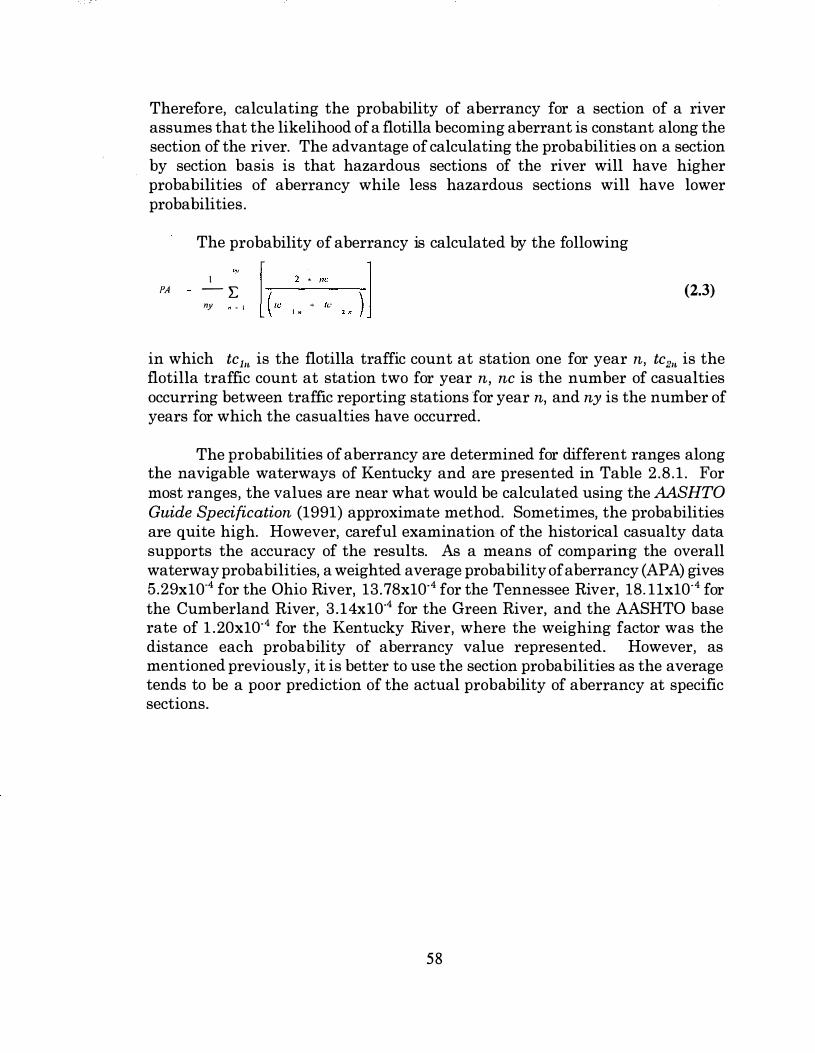
Therefore, calculating the probability of aberrancy for a section of a river assumes that the likelihood of a flotilla becoming aberrant is constant along the section of the river. The advantage of calculating the probabilities on a section by section basis is that hazardous sections of the river will have higher probabilities of aberrancy while less hazardous sections will have lower probabilities.
PA
The probability of aberrancy is calculated by the following
I - I; ny n � I
(2.3)
in which tc1" is the flotilla traffic count at station one for year n, tc2" is the flotilla traffic count at station two for year n, nc is the number of casualties occurring between traffic reporting stations for year n, and ny is the number of years for which the casualties have occurred.
The probabilities of aberrancy are determined for different ranges along the navigable waterways of Kentucky and are presented in Table 2.8.1 . For most ranges, the values are near what would be calculated using the AASHTO Guide Specification (1991) approximate method. Sometimes, the probabilities are quite high. However, careful examination of the historical casualty data supports the accuracy of the results. As a means of comparing the overall waterway probabilities, a weighted average probability of aberrancy (AP A) gives 5.29x10.4 for the Ohio River, 13. 78x10'4 for the Tennessee River, 18. 1lx10'4 for the Cumberland River, 3.14x10'4 for the Green River, and the AASHTO base rate of 1 .20x10'4 for the Kentucky River, where the weighing factor was the distance each probability of aberrancy value represented. However, as mentioned previously, it is better to use the section probabilities as the average tends to be a poor prediction of the actual probability of aberrancy at specific sections.
58

Table 2.8.1: Probability of Aberrancy for Rivers in K t k en uc �:y.
I
River Miles Below Pittsburgh for Probability of Aberrancy Ohio River and below the Ohio for all Other Rivers
279-341 4.495xl0''1
341-436 1.770x10"4
436-531 6.579x10'4
531-606 10.424xlO··I
606-720 3.030x10''1 Ohio
720-776 2.029x10⁻⁴
776-846 3.432x1o·<
846·918 3.638xl0''1
918-938 15.283x1o··•
938-mouth 13.716xl0'4
000-099 16.835xl0'4
099-206 15.687xlO"'
206-259 9.485xl0"1
259-274 5.272xl0'4
274-349 15.298xl0'4 -
Tennessee 349-424 10.840x10''1
424-471 13.19lxl0'4
471-529 7.639xlo··l
529-570 11.41 1xlO··I
570-602 27.548xl0''1
602-652 13.636xlo··l
000-030 18.582x10''1
030-075 40.738x1o··' Cumberland
075-148 2.666x10'4
148-216 19.520x10''1
Green all 3.140xl0'4
Kentuc� all 1.200x10"1
There are no known casualties along the Kentucky River; therefore, the AASHTO minimum probability of aberrancy of 1.200x10'4 was used.
59
2.9 DESIGN BARGE ACCEPTANCE CRITERIA
Method II of the AASHTO Guide Specification is a probabilistic design methodology. In this method, the possibility that a barge flotilla impact with a bridge will cause failure is deemed acceptable provided the probability of the failure of the bridge is extremely low. Section 4.8.2 of the AASHTO Guide Specification recommends that the design flotilla be selected in accordance with the following acceptance criteria for the total bridge:
• CRITICAL BRIDGES. The acceptable annual frequency of collapse, AF,, of critical bridges shall be equal to, or less than, 0. 01 in 100 years (AF=AF,=O. 000 1).
• REGULAR BRIDGES. The acceptable annual frequency of collapse, AF, of regular bridges shall be equal to, or less than, 0. 1 in 100 years (AF=AF,.=O. 00 1).
It is recommended that the definition for a critical bridge be the same as the definition for an essential bridge as given in the FHWA Seismic Retrofitting Manual For Highway Bridges. An essential bridge, as defined in the Retrofitting Manual, satisfies one or more of the following conditions:
• a bridge that is required to provide secondary life safety; e.g., a bridge that provides access to local emergency services such- as hospitals. This category also includes those bridges that cross routes which provide secondary life safety, and bridges that carry lifelines such as _ electric power and water supply pipelines;
• a bridge whose loss would create a major economic impact; e .g., a bridge that serves as a major link in a transportation system;
• a bridge that is formally defined by a local emergency plan as critical; e.g., a bridge that enables civil defense, fire departments, and public health agencies to respond immediately to disaster situations. This category also includes those bridges that cross routes which are defined as critical in a local emergency response plan and those that are located on identified evacuation routes; or
• a bridge that serves as a critical link in the security/defense roadway network.
All other bridges not satisfying one or more of the above definitions should be classified as regular bridges.
60

The acceptable annual frequency of bridge collapse is distributed, either equally or at the designers discretion, over all piers that are located within the waterway. However, it is recommended that the annual frequency of collapse (AF) be distributed to each pier based on its percentage value of the replacement cost of the structure. For example, the annual frequency of collapse for a pier (AFP) which constitutes 25 percent of the replacement cost of a critical bridge (AF=AF,) would be:
AF AF
0 . 0001
4 4 0 . 000025 (2.4)
The summation of the annual frequencies of collapse for all barge size categories, with respect to the individual piers, should then be less than or equal to the AFP assigned to each component. In addition to the probability of aberrancy provided in the previous section, the data required for calculating the annual frequencies of collapse for all barge size types can be generated using the same procedure as outlined in the Maysville Design Example of Appendix I.
6 1

2.10 SCOUR REQUIREMENTS
The current AASHTO Guide Specification does not provide guidance on the application of scour to the barge impact design of bridges. However, in a letter dated September 4, 1992 the FHWA Region 4 office directed the application of the following scour conditions to impact design using the AASHTO Method II procedures:
1 . For impact loads applied at normal vessel operating conditions, two scour conditions should be evaluated. The first is the scour having a probability of 1.0, most likely only the long-term scour plus the contraction and local scour caused by a Q5 event. The second is the maximum anticipated scour (or other critical value determined by the designer). The probability of this scour occurring during the life of the bridge should be included in the calculations.
2. For the case of the free-floating empty barge on the 100-year flood, the maximum anticipated scour should be used.
Therefore, it is recommended that the impact loads for the loaded barge flotillas be applied in conjunction with 100% of long-term scour plus the local scour caused by a Q5 (five-year return period) flood event. The impact loads for a single free-floating barge should be applied with the scour caused by the Q100 flood event plus 100% of the long-term scour. Appendix I contains a design example which illustrates this application.
2_1 1 SUMMARY AND CONCLUSIONS
A method has been provided by which available barge and flotilla data may be utilized to develop the risk assessment procedures for vessel impact design problems in accordance with the 1991 AASHTO Guide Specification. For illustrative purposes, this study concentrated on barge traffic on Kentucky's navigable waterways. However, the methods presented in this study are applicable to all navigable inland waterways. Results generated in this study reflect a statistical analysis conducted on the data obtained from the U.S. Coast Guard, the U.S. Army Corps of Engineers, and the American Waterways Operators. The data gathered in order to apply design Method II of the guide specification are: 1) barge size and capacities, 2) the number of barges in a flotilla column and row, 3) river elevations, 4) flotilla transit velocity, and 5) probabilities of aberrancy.
62

The barge types defined in this study are based on the U.S. Army Corps of Engineers' barge length and width designation system. Flotillas are generally made up of mostly the same barge size and type. Nevertheless, it was found that a very large variation in the flotillas using the Kentucky waterway system still exists. Therefore, a probability based approach was adopted to calculate the number of barges comprising a flotilla. Flotillas are then categorized based upon the primary barge type in the train.
Maximum attainable speeds for fully loaded flotillas under ideal conditions, as determined by a survey of the American Waterways Operators and the U.S. Coast Guard Captain of the Port, Louisville, KY, are reported. Values used for flotilla transit velocity are: 1) 7 mph for the Ohio and Tennessee Rivers, and 2) 5 mph for the Cumberland and Green Rivers. Since, the Performance Monitoring System Database does not currently document any flotilla traffic on the Kentucky River, the minimum value of 5 mph should be used for flotillas navigating this river.
The probabilities of aberrancy have been reported for different ranges along the navigable waterways of Kentucky in other sources. For most ranges, the values are near what would be calculated using the AASHTO Guide Specification (1991) approximate method. Sometimes the probabilities are quite high. However, careful examination of the historical casualty data supports the accuracy of the results. It is recommended that the probability of aberrancy for a section of river under consideration be used in design calculations, instead of a weighted average PA for the entire river.
Based on section 4.8.2 of the AASHTO Guide Specification (1991), the acceptable annual frequency of collapse, AF, was reported as 0.0001 for critical bridges and 0.001 for regular bridges. The acceptable annual frequency of bridge collapse should be distributed, either equally or at the designer's discretion, over all piers located within the waterway. A recommendation to distribute the annual frequency of collapse to each pier based on its percentage value of the replacement cost of the structure was reported. The summation of the annual frequencies of collapse for all barge size categories, with respect to the individual piers, should then be less than or equal to the AFP assigned to each component.
It is recommended that the impact loads for the loaded barge flotillas be applied in conjunction with 100% oflong-term scour plus the local scour caused by a Q5 flood event. The impact loads for a single free-floating loaded barge (as per the Kentucky Transportation Cabinet design minimum assumption) should be applied with the scour caused by the Q100 flood event plus 100% of the longterm river bed aggravation or degradation. Currently, the AASHTO Guide
63

Specification gives no guidance for using future barge traffic projections when considering the design life of the bridge. Therefore, it is recommended that a 50 year design life be used.
The lateral capacities of the bridge piers required using design Method II of the AASHTO Guide Specification (1991) are found to be more conservative than the lateral capacities required using the less rigorous design Method I procedure. However, the results of this study indicate that, after the initial effort by a state or agency of accumulating and processing the necessary information, further designs using Method II can be completed with economy equal to designs completed using Method I.
The equivalent static impact loads and their associated frequencies are derived for a bridge over the Ohio River. The impact loads calculated using the currentAASHTO formulas probably give unrealistic results since they are based on relationships which neglect energy dissipation due to crushing and friction and dynamic load magnification effects. The following Sections of this report present analysis procedures which include the effects of the dynamic interaction between the individual barges in the flotilla and the bridge pier. The example given in Appendix I illustrates the use of the probability procedures given in this Section used in conjunction with the current equivalent static load analysis procedure. The current analysis method was used in place of the suggested analysis methods (given later) so as to provide a clear example of the application of only the methods given in this Section.
64
3.0 BARGE IMPACT LOADING FUNCTIONS AND IMPACT SPECTRUMS
3.1 INTRODUCTION
The current method of analysis of bridge piers subjected to vessel impact, called the equivalent static method (Section 3.12, AASHTO Guide Specification and Commentary for Vessel Collision Design of Highway Bridges), involves a great number of simplifications and assumptions on the part of the engineer. This is due to the complexity of the problem. The true dynamic structural response due to the load time-history is approximated by an assumed equivalent static response. The main drawback with the current method is that it ignores the dynamic interaction between the individual barges and the bridge during the collision. The resulting design may at best be excessively costly, or more importantly may be susceptible to catastrophic failure.
The purpose of this and the next Section is to develop a single inertial mode design method which models the dynamic interaction between the individual barges in the flotilla and the bridge during the collision. The resulting design procedure will be called the Pseudo-Dynamic Analysis Procedure (PDAP). The development of a second design procedure which includes multiple inertial modes is given in Appendix III and is called the Impact Spectrum Analysis Procedure (ISAP). However, before developing these two design procedures it is first necessary to derive a method to calculate the impact time-histories for single and multiple barge impacts, and derive the subsequent impact spectrums for these impact time histories. The impact timehistories and impact spectrums will be derived within this Section. The flow chart given in Figure 3.1 .1 details the procedure used in this Section to develop the impact loading functions and impact spectrums.
65
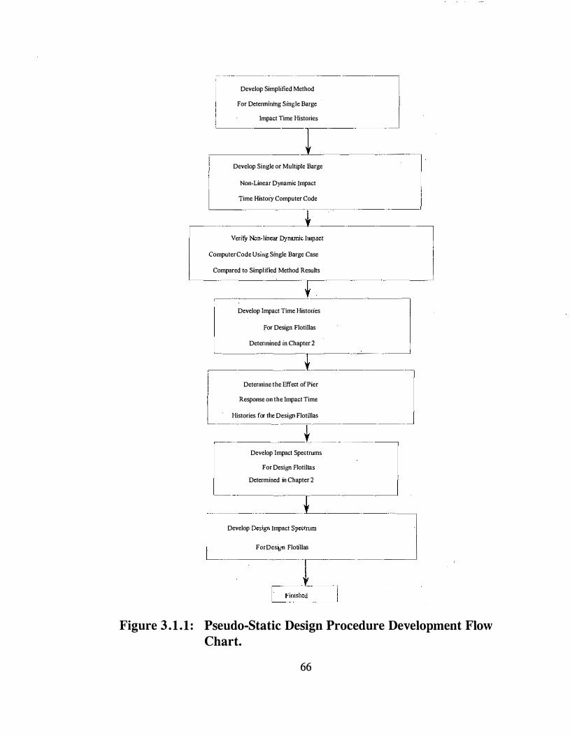
Develop Simplified Method I For Detenmnmg Smg:le Barge I
Impact Time Histones J r----Develop Single or Multiple Barge
-----
I Non-Linear Dynamic Impact �ime Hi•tory Computer Code ... . . .. -
V
enzy Non-;meM-��':!." --=- --�
omputer Code Usmg Smgle Barge Case
Compared to S1mphfied Method Results
. _ __ 1-----·· Develop Impact Time Histories
For Design Flotillas
Detennined in Chapter 2 II·�
l ,-------- ··-{___
--·
I Detennine the Effect of Pier
L Response on the Impact Time · Histories for the Design Flotillas
=-==��--t _ _ _ _
I D"dop Im
.
pact Speotrum•
...
_j For Desi�:,m Flotillas
Determined in Chapter 2 ·--L Develop �e��gn Impact :p:trum
--------- ···-1
Fa<Desib"' Flotill" _j � -I-- -[!inished
-· _j Figure 3 .1 .1 : Pseudo-Static Design Procedure Development Flow
Chart.
66

3.2 FLOTILLA AND BARGE SIZE DISTRIBUTIONS
In order to determine the barges and flotillas for which the loading functions and impact spectrums are needed for a particular bridge site, an assessment of the barge traffic using the waterway would need to be conducted (Section 3.3, AASHTO Guide Specification). Typically, such an assessment would require significant engineering hours. However, Section 2 determined the design flotillas and their respective frequencies at intervals along all navigable rivers in Kentucky.
Therefore, the impact spectrums and loading functions for a bridge over a Kentucky waterway would be developed for the design flotillas, for the appropriate section of waterway, identified in Section 2. Initially, for verification of the computer code, a single barge loading function will be developed. Extension of the procedures to the realistic multi-barge flotilla will be presented in subsequent sections.
3.3 BARGE IMPACT LOADING FUNCTIONS
The first step in the derivation of the PDAP and ISAP, as given in Figure 3 .1 .1, is the determination of the flotilla impact loading functions. Based on past flotilla-bridge collision investigations, AASHTO recommends only the barges in a single column of a multi-column flotilla be used in developing the impact loading (Section C3. 12, AASHTO Guide Specification) since barges in adjacent rows are lashed together with ropes that break during the collision. It would be assumed that additional columns would break loose on impact and would not substantially contribute to the impact load applied to the bridge. Figure 3 .3 .1 gives the flotilla row and column definitions. The single-barge loading function presented in the following sections will utilize the barge loaddeformation test results used for the AASHTO barge impact design formula (Section 3. 12, AASHTO Guide Specification). A more detailed discussion of the AASHTO equation and load deformation curve will be given in a later section. The procedure can be used to develop a loading function for whatever configuration is selected for the design flotilla column.
Two methods are employed to develop the single barge impact loading functions. The first method is a numerical technique using the AASHTO bilinear barge load-deformation model at the contact zone between the barge and the bridge. The second method is a finite element model that uses the AASHTObilinear barge load-deformation crushing zone stiffness in conjunction with a lumped or consistent mass dynamic analysis.
67

3.3.1 Simplified Model: Barge Loading Function
The first procedure used to derive the barge impact loading functions is a simplified method. In order to develop the loading function using a simplified barge model, it is assumed the barge impinges perpendicularly on a rigid support (pier). If it is further assumed that the support crushes only the section of the barge adjacent to the support, the barge may be divided into two regions; (1) a non-linear crushing zone, and (2) a rigid zone (Figure 3.3.2).
The barge impact force, F , on the rigid bridge pier may be written
dM F , (3.1) dt
where, dM/dt is the change in momentum of the barge with respect to time. If the change in momentum is written as the difference between the momentum at t = t, and t = tn+1 the resulting impact force may be written
F , M - M
dt " • I
(3.2)
where, M, is the momentum of the total system at t = t,, and M,+1 is the momentum ofthe total system at t = tn+J· Furthermore, the momentum at times t, and tn+1 can be expressed as
M M " . 1
m x· ( m dm ) ( X - d X )
(3.3a) (3.3b)
where, m, is the uncrushed mass at time t,, dm is the crushed. mass at time t,+1,
" is the velocity of the uncrushed mass at time t,, and d " is the change in
velocity ofthe mass over the time increment t,.1 - t,. Substituting Eqn. 3.3 into Eqn. 3.2 gives
d i dm dm F "' m - · x -- - d x --dt dt dt
(3.4)
68

where the term d ,. d , , d , is small compared to the other terms and may be
neglected giving
d x' dm F "' m - · x -
dt dt (3.5)
It can be seen by examining Eqn. 3.5 that the first term on the right-hand side represents the force on the pier due to the deceleration of the barge mass which is a function of the crushing element resistance, f(x) ,which is dependent on the deflection, x(t), and is written
d x: m - "' f ( x )
dt (3.6)
Moreover, the instantaneous change of the mass due to crushing in the second term on the right-hand side of Eqn. 3.5 can be written as
drn tn ( x ) :i (3.7) dt
where "' , , J is the mass density distribution function along the barge length (mass per unit length). Substituting Eqns. 3.6 and 3. 7 into 3.5 results in
' F = f ( x ) + m ( x ) :i (3.8)
In order to solve Eqn. 3.8 relationships for the displacement, velocity and acceleration are needed. The relationship for the acceleration is obtained by writing the deceleration of the uncrushed mass of the barge as
f ( x ) L (3.9)
J "' m ( x ) dx
{ ( X ) ;i' o ------ (3.10) m ( L - x )
69
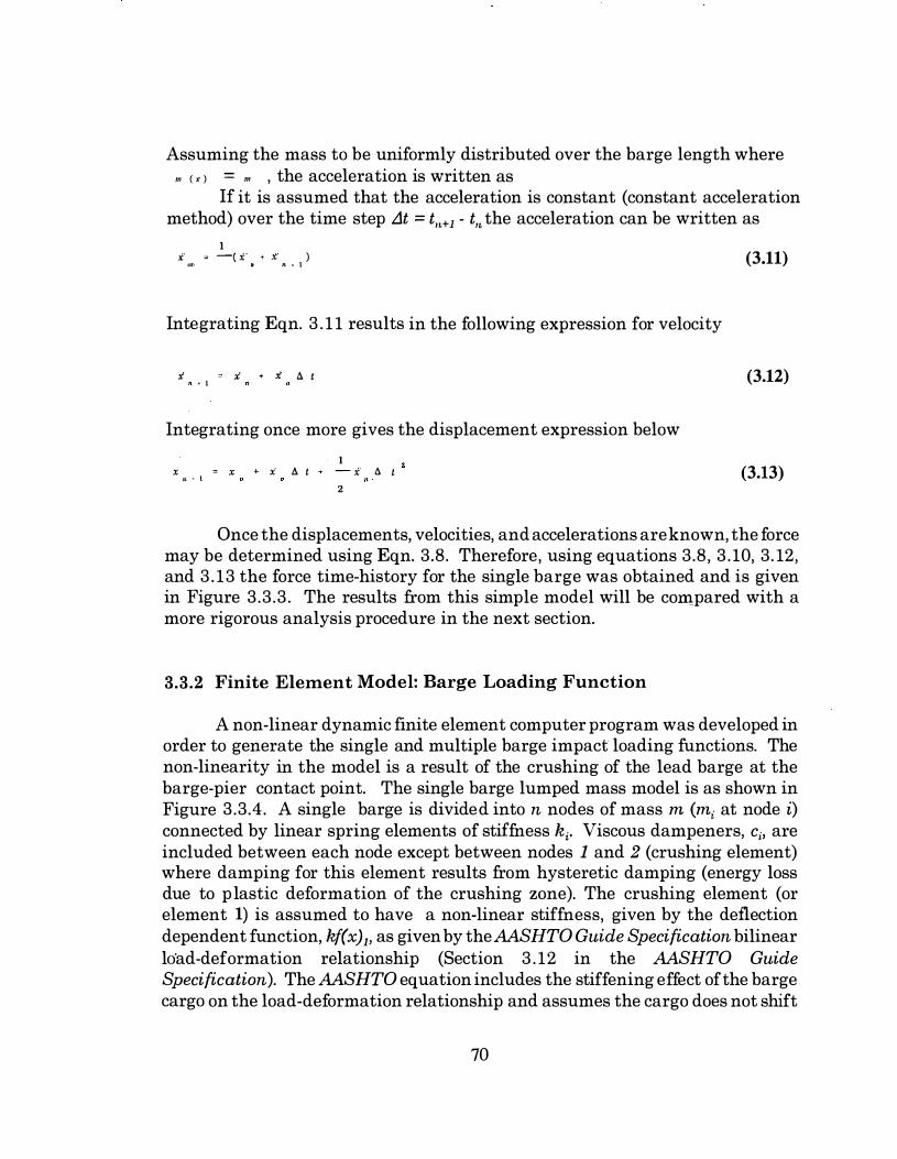
Assuming the mass to be uniformly distributed over the barge length where m ( ' ) = m ' the acceleration is written as
If it is assumed that the acceleration is constant (constant acceleration method) over the time step Lit = t,.+1 - t,. the acceleration can be written as
I x: = -c x· + x: ) "'' • n • I
Integrating Eqn. 3 .11 results in the following expression for velocity
i :i + i' !::. t " . '
Integrating once more gives the displacement expression below
X "' X " . I I
x a t - x· ll t 2
(3.11)
(3.12)
(3.13)
Once the displacements, velocities, and accelerations are known, the force may be determined using Eqn. 3.8. Therefore, using equations 3.8, 3 .10, 3. 12, and 3.13 the force time-history for the single barge was obtained and is given in Figure 3.3.3. The results from this simple model will be compared with a more rigorous analysis procedure in the next section.
3.3.2 Finite Element Model: Barge Loading Function
A non-linear dynamic finite element computer program was developed in order to generate the single and multiple barge impact loading functions. The non-linearity in the model is a result of the crushing of the lead barge at the barge-pier contact point. The single barge lumped mass model is as shown in Figure 3.3.4. A single barge is divided into n nodes of mass m (mi at node i) connected by linear spring elements of stiffness ki. Viscous dampeners, ci, are included between each node except between nodes 1 and 2 (crushing element) where damping for this element results from hysteretic damping (energy loss due to plastic deformation of the crushing zone). The crushing element (or element 1) is assumed to have a non-linear stiffness, given by the deflection dependent function, kf(xh as given by the AASHTO Guide Specification bilinear load-deformation relationship (Section 3 .12 in the AASHTO Guide Specification). The AASHTO equation includes the stiffening effect of the barge cargo on the load-deformation relationship and assumes the cargo does not shift
70

during impact. The barge impinges on a bridge pier of mass mP, stiffness kP (formulated to include a non-rigid pier), and damping coefficient, cP.
The global damping matrix, [C] , is assumed to be of the Raleigh Damping form, such as
[ C J · • I M I • P I K I (3.14)
where, [M] is the global mass matrix, [K] is the global stiffness matrix, and a and P are usually determined such that the damping ratio of two widely spaced modes contributing significantly to the response is 5% of critical (Clough, Penzien, 1993). Within this Section the mass and stiffness matrices are both non-linear (i.e . , not constant). However, the damping matrix is assumed constant, where the initial mass and stiffness matrices are used in Eqn. 3. 14.
As a conservative approach, only longitudinal translation is included in this model. The linear stiffness elements work in tension and compression. The spring (crushing element) force, f(x), contacting the pier support uses the barge load-deformation hysteresis shown in Figure 3.3.5. The curve uses the AASHTO bilinear load-deformation curve and assumes elastic unloading and reloading over the elastic deformation range, 0.34' (0. 1 meter), as given by the Guide Specification. The current model allows only contact compression and utilizes a bilinear static load-deformation relationship derived from single barge impact tests . Contact compression necessitates the inclusion of rigid body mode translation if the pier and impinging flotilla separate during the collision (Figure 3.3.5c). When rigid body modes are included and the velocities and accelerations approach zero, numerical stability must be maintained to ensure a non-singular effective dynamic stiffness matrix. This is achieved by maintaining a small stiffness for the crushing element of k" xl o·4, where k" is the elastic crushing element stiffness.
3.3.2.1 Crushing Element
The mass of the crushing element changes over the time increment Lit as a result of crushing. The change in the mass (mass units only) over the time interval over the time step Llt=tn+J - t., is
11 m = m [ ( l - q, } x' + lj> x' ] !J. t " n • l (3.15)
where, <1> = weighting factor dependent on the time integration scheme, is the
7 1

velocity at time tn, and · , . , is the velocity at time tn+I. However, for a small time interval, llt, giving a small change in the velocity over the time step, Eqn. 3 .14 can be written
A m , m X A t "
(3.16
The change in the crushing element mass 11m over the time interval llt is assigned to the pier node at the end of the time step and the crushing element nodal lumped mass are recalculated.
The force on the support node as a result of the change in momentum of crushed mass, F,, over the time interval is
A "' ( X " ) " • I F 0 (3.17)
A t
Therefore,
F 0 "' " ( " - x ) " • I " (3.18)
The total impact force on the support node is then a result of the barge crushing mass and the barge crushing resistance and is written
F = f ( x ) + m X ( :i " , I i ) (3.19)
where f(x) is the barge load deformation force taken from the bilinear load deformation relationship (Section 3. 12, AASHTO Guide Specification) described previously. Since the load deformation hysteresis is non-linear, an incremental time discretization procedure was utilized for the solution of the equation of motion.
3.3.2.2 Dynamic Equilibrium
The equation of motion may be written at times t = tn and t = tn+Jo respectively as follows
72
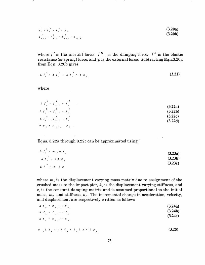
I D $ 1 , + 1 I , " P (3.20a)
(3.20b)
where f r is the inertial force, f n is the damping force, f s is the elastic resistance (or spring) force, and p is the external force. Subtracting Eqn.3.20a from Eqn. 3.20b gives
I II S !:J. f + !:J. { + !:J. { !:J. p n I ,,
where
" f "
f " . l
f " l> " l>
" f " f " . ' f " s s s
" f "
f " . l f "
" p p " � l p
Eqns. 3.22a through 3.22c can be approximated using ·
I !:J. f , = m !:J. x·
l> !:J. f ,. = c 6 :i
s 6 { " k !:J. X
(3.21)
(3.22a) (3.22b) (3.22c) (3.22d)
(3.23a) (3.23b) (3.23c)
where m,. is the displacement varying mass matrix due to assignment of the crushed mass to the impact pier, k,. is the displacement varying stiffness, and c,. is the constant damping matrix and is assumed proportional to the initial mass, m1 and stiffness, k1• The incremental change in acceleration, velocity, and displacement are respectively written as follows
" :i" 0 i:" :i" " '
" " 0 " " " '
" X 0 X - X " '
m 6 i" + c !:J. :i k !:J. X 6 p
73
(3.24a) (3.24b) (3.24c)
(3.25)

Substituting Eqns. 3.23 and 3.24 into Eqn. 3.21 gives or in matrix notation
[ M ( x ) ] l ll i" ! + [ C ] l ll .i ) + [ K ( x ) ] ! 8 x ) " ( 6. P ( t ) J (3.26)
where [M(x)] is the non-linear global mass matrix dependent on the displacement, x, [K(x)] is the non-linear stiffness matrix dependent on the deflection, [C] is the constant damping matrix proportional to the initial mass and stiffness, and {LlP(t)} is the external time loading function vector. However, since the barge impact problem is an initial value problem, i.e . , {LlP(t)} = {0}, Eqn. 3.26 becomes
[ M ( x ) ] l ll :r: l + [ C ] { I:J. x' l + [ K ( x ) ] l tJ. x l "' 0 (3.27)
It is important to note that in Eqn. 3.27 the damping matrix, [C], is assumed as constant. This assumption is utilized in this study since damping in non-linear elements experiencing significant irreversible strain will be dominated by hysteretic damping and any error introduced by utilizing a constant damping matrix will be insignificant (Blandford, and Glass, 1987)
The Wilson-8 method was used for step-by-step integration of the nonlinear equations of motion. The basic assumption of the Wilson-8 method is that the acceleration varies linearly over an extended time step such that the extended time interval s is given by
s = e A t (3.28)
Nickell (1971) demonstrated that 8 must be greater than 1.37 to ensure unconditional numerical stability. Bathe (1981) further showed that the optimum value of 8 is 1.420815 which is the value used in the formulation given here. Using the linear extended time step assumption, it can be written
' 11 x c t ) = s :l ( t ) + -tJ. x· c t )
2
' ' a x ( l ) s x c t ) + - :{ ( t ) + -tJ. x· c l )
2 6
(3.29a)
(3.29b)
74

where IJ. X ( t ) � X ( t + 5 ) X ( t )
(3.30a) IJ. t ( t ) " x' ( t + 8 ) X ( t ) (3.30b)
(3.30c) !J. :f ( t ) " x: ( t + 8 ) - x: ( t )
Solving Eqn� 3.30 for the incremental velocity and acceleration in terms of the incremental displacement gives
6 6 a l :i" ( t ) l = - tJ. l x ( t ) l - - l t ( t ) l - 3 l :t:" ( t ) l
3 ' A l .r ( t ) ) = - a { x ( t ) l - 3 U ( t ) l - - { :C" ( t ) l
2
Substituting Eqn. 3.31 into Eqn. 3.26 gives
where
[ K · ( x ) j 3
[ K ( x ) 1 -r - [ C 1 6
- [ M { r ) ]
and
(3.31a)
(3.31b)
(3.32)
(3.33)
(3.34)
Equation 3.32 can then be solved for the displacement increment that is used in Eqn. 3.3la to solve for the acceleration increment. Using the results from Eqn. 3.3la, the incremental acceleration is found from
1 IJ. l i' l = -o. t x· 1 (3.35)
•
where , is the acceleration over the extended time step, s. The velocity and displacement at the end of the time increment are found from
• t l .i ( t + A t ) l = l X ( t ) l + A t l .:f ( t ) l +
,- l i: ( t ) l
ll t A t 2 l x' ( t + !J. t ) l = l x ( t ) l + !J. t l :i ( t ) l + -- { t" ( t ) ) + -- { x: ( t ) l
6
75
(3.36a)
(3.36b)
To ensure dynamic equilibrium, the acceleration is calculated from
{ .t' ( t + A t ) l " [ M ( t + A t ) ] - 1 [ - F ( t + .6. t ) - F ( t + A t ) ]
• (3.37)
The results from Eqns. 3 .36 and 3.37 give the initial conditions for the next time step. This solution strategy is utilized to compute the barge impact loading functions of the next sections.
It is important to note that since both the stiffness and mass matrices are non-linear, exact direct solution of Eqn. 3.32 is not possible. Rather, an iterative solution technique must be used in order to approach the exact solution. Within the goal of this Section, which is to determine a reasonable approximation of the barge flotilla impact force time-histories, a nearly exact solution of the problem formulation has little significance. Especially in light of the fact that the actual load-deformation behavior of the barges are not known with a high degree of certainty. Therefore, the direct integration approach to the solution of Eqn. 3.32 is adopted in this Section as compared to the iteratitive solution techniques used later in Sections 5 and 6.
The direct integration approach assumes that the system properties (i.e., stiffness and mass) over the load increment. The mass and stiffness matrices are updated at the beginning of each load step. This approach introduces an error in the overall solution as can be seen by the single degree of freedom example shown in Figure 3.3.6a. However, significant divergence from the actual solution may be avoided by using small load steps and reformulating the system properties before proceeding to the next solution step.
The direct integration approach is utilized here where the load is applied in small increments as determined by the small solution time steps. The small divergence from the actual solution for a single degree-of-freedom system is shown in Figure 3.3.6b. Accuracy of the solutions achieved using the direct integration approach in this Section was checked by using increasingly small time steps until apparent convergence was achieved in the solution. An arbitrary solution tolerance for determination of the peak impact load of 1% was used for all load time-histories calculated. The following sections detail the single and multiple barge load time-histories determined using the preceding fo r m u l a t i o n .
76

(j) :s 0
Ct:
QJ 01 '--0
m
'+-0
L QJ
_[) E :J
z
y
-<(- -----
' ' ' N B r-,r_l\ Tn•
Figure 3.3.1: Barge Flotilla Column and Row Definitions.
77

t = t
t = t
t = t "'
..,c---- -------- L -
X
"""(---- L - u
I '
X - !; X
"' Rigid Zone
..-------·--- L - u "'
-<-- - ---
X - l!J. X
Rigid Zone
""
.
_________ ,..
_____ ,..
Crushing Zones
Figure 3.3.2: Simplified Barge Impact Model.
78
X

2500
2000
,--, "' � '-'
(500
<l) 0 15 1000
�
500 . . . . . . . . . . . . . . . . . . . . . . . . . . . . . . . . . . . . . . . . . . . . . . . . . . . . . . . . • . . . . . . . . . . . . . . . . . . . . . � . • . . . . . . . . .
0
0.00 0.25 0.50 0.75 1.00
Time (sec)
Figure 3 .3.3: Force-Time Relationship for a Single 35'x195' Barge Neglecting the Effect of Pier Flexibility on the TimeHistory.
79

<(----·--- ------------------.. �·--· -� -)>
c n
k
c 3 \
Figure 3.3.4: Single Barge Non-Linear Lumped Mass Impact Model.
80
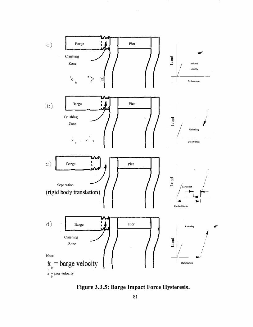
n ) Barge
CrUshing
Zone
X "> X b
( b ) Barge
Crushing Zone
X X p b
c ) I Barge
0 Separation
(rigid body translation)
d )
Note:
Barge
Crushing Zone
xb = barge velocity x = pier velocity
p
Pier
Pier
Pier
Pier
Inelastic I Loading
----- --
Dcfurrnnlion
/ !
"g I 0 r .....1 I
I Unloading
· · --·---
Dcfonnntion
"g 0 .....1 I Supomllon 1
_
--�---�-�L= Crushed D�pth
Reloading
Deforrnation
.,. l
f I
I
Figure 3.3.5: Barge Impact Force Hysteresis.
81
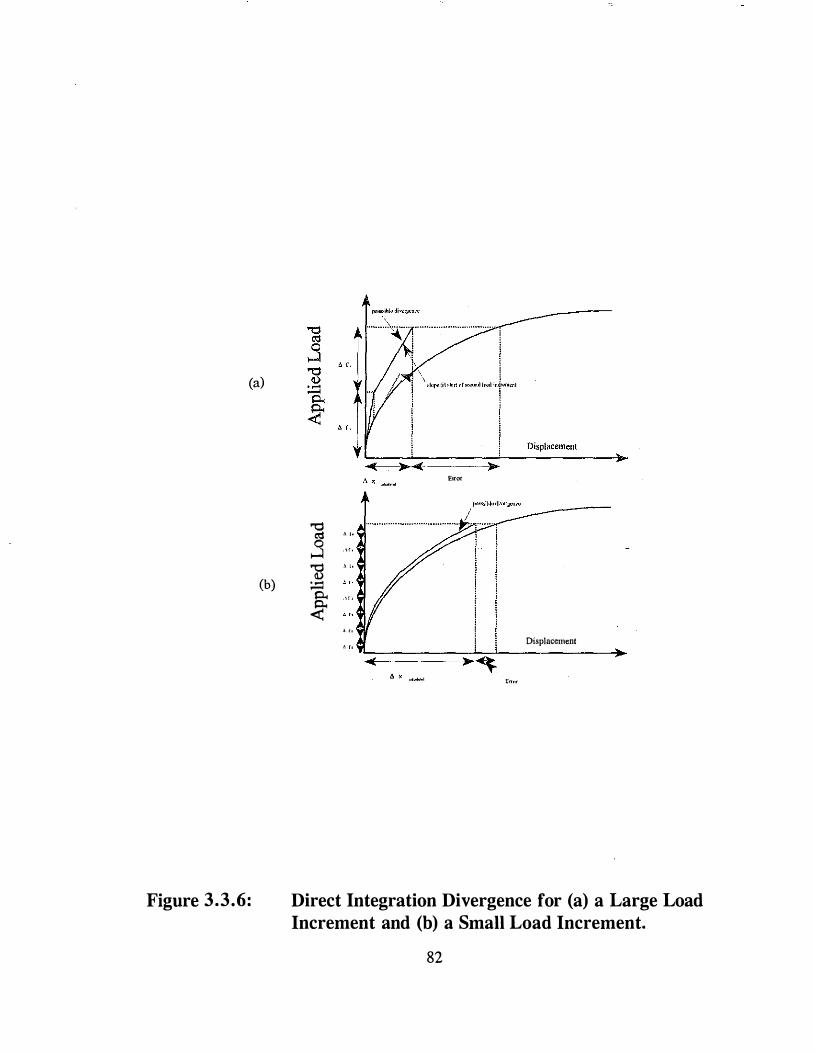
(a)
(b)
Figure 3.3.6:
"d o; 3 "d 0 ;.::l 0.. <
Y ����----��--D-i•_PI_"_'m_'"_' --�� _____ ,..� --->-Error
. ..
,,f,
' "
" '
, \ f >
, ,, .
Displacement
�"'"
Direct Integration Divergence for (a) a Large Load Increment and (b) a Small Load Increment.
82

3.4 SINGLE BARGE IMPACT LOADING FUNCTIONS
The previously described computer program was utilized to develop the loading function for a single 35'x195' barge. Typically, for design purposes impact loading functions would be developed for the design barge configurations determined by the statistical analysis of Section 2. However, for verification of the computer code the single barge case is developed first.
The axial barge element stiffness was calculated from the cross-sectional properties of a 35'x195' cargo barge as provided by the U.S. Coast Guard, and the load-deformation hysteresis previously given in Figure 3.3.5 was used for the crushing element stiffness. The mass of the barge used includes the cargo mass which is assumed to be distributed uniformity along the barge length. The barge was discretized into 19 elements each ten feet in length, with exception of the first element (crushing element) which is 15 feet in length. The results from the computer program and the previously given approximate method (section 3.3.1) are illustrated in Figure 3.4.1 and show excellent agreement between the two methods.
83
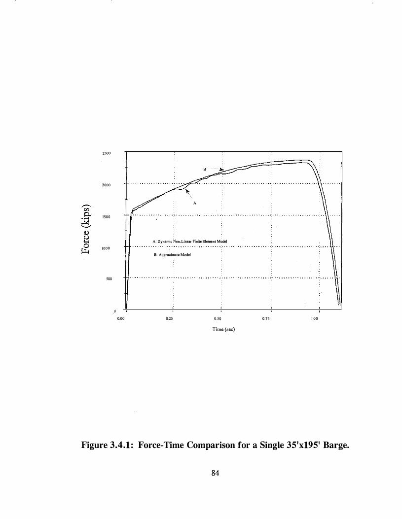
2500
2000
1500
A: Dynamic Non-Linear Finite Element Model
1000 B: Approximate Model
500
0.00 0.25 0.50 0.75 1.00
Time (sec)
Figure 3.4.1 : Force-Time Comparison for a Single 35'x195' Barge.
84

3.5 MULTIPLE BARGE IMPACT LOADING FUNCTIONS
The multiple barge impact loading time-histories for the flotilla types given in Section 2 were developed utilizing the previously given time-history analysis code. The barge load-deformation curve from the AASHTO Guide Specification was used for each of the individual barges comprising the flotilla column. A mass and stiffness discritization is shown for the multi-barge impact model in Figure 3.5.1.
As was the case for the single barge model, the axial barge element stiffness for each barge in the flotilla was calculated from the cross-sectional properties of a 35'x195' cargo barge. The mass of each barge used includes the cargo mass which was assumed to be distributed uniformity along the barge length. In addition, each barge was discritized into 195 elements each one foot in length, where the first element is initially the crushing element, The crushing element for each barge is allowed to crush one-half its length and then is assigned an elastic stiffness equal to 100 times the linear element stiffness. The next element then becomes the crushing element and is, in turn, allowed
to crush one-half its length and so on.
The mass matrix of each crushing element is not modeled as being constant. Instead, as the element crushes, the mass proportional to the change of the crushing element length is concentrated at the node at the interface of the crushing element and the adjacent element. The mass concentration process was given previously by Eqn. 3.18 and results in a force on the bridge or the next barge. The force is produced from the change in momentum of the barge and the barge cargo due to the deceleration of the mass during crushing.
Within the model, the individual barges are assumed to have direct contact with each other (i.e. no rubber bumpers). In addition, five percent Rayleigh damping is assumed for the linear (non-crushing) elements. A crushing element is assumed initially as the first element of each barge which is assigned the AASHTO bilinear load deformation relationship and the loading and unloading hysteresis shown in Figure 3.5.2. The impact time-histories were developed for one through four fully-loaded 35'xl95' barges and are given in Figure 3.5.3. A comparison of the results given by Figure 3.5.3 and the current AASHTO equations will be given in the following section.
85

� i .� (L .
w "' 0
(I)
m !I
'
Jl
J
J
Figure 3.5.1: Multiple Barge Non-Linear Lumped Mass Impact Model.
86

o )
( b ) E� t:l r-�] 8 r 1
C r · u ::.; h i n q
z (, n e
X
I
C r·u :::; h i n q
z(,ne
X , ' X
n
n
n-1
C r u s h i n�J
Z u n e
, X n - l
I a o rg e � St-; p t:l (i:J l i t:'n
(rigid body translation)
cl ) C r u ::.; h i n q
Zt :, n e
8 u r""�Je n - 1
C r· u ::; h i n�J
Z n n e
Deformation
1l 0 ..-1
Defonnntion
53 1 1l 0 ..-1
Crushed Depth
Defurmntion
Figure 3.5.2: Multiple-Barge Interaction Hysteresis.
87
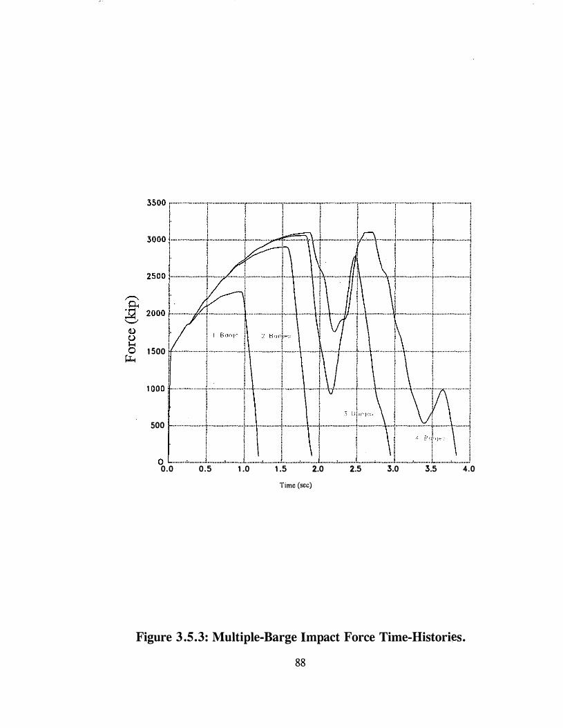
1 500
500
0.0 0.5 1 .0 1 .5 2.0 2.5 3.0 3.5 4.0 Time (sec)
Figure 3 .5.3: Multiple-Barge Impact Force Time-Histories.
88

3.6 COMPARISON OF TIME-HISTORY AND AASHTO METHODS
A direct comparison of the impact time-histories and the equivalent static loads predicted by the equations of section 4.2.1 of the AASHTO Guide Specification do not have a great deal of significance since the AASHTO equations do not consider the loading history and only predict the peak point on the loading time-history. Therefore, the dynamic effects of the barge impact are neglected by the AASHTO equations. A means of comparison can be afforded by comparing the peak load predicted by the impact time-histories and the AASHTO equivalent static load.
The comparison of the loads for a single barge predicted by the equivalent static method and the time-history method is given in Figure 3.6.1. The peak load predicted by the AASHTO method is within 5% of the peak load predicted by the time-history. However, as Figure 3.6.2 reveals, the peak load for the four-barge column predicted by the equivalent static method is 44% greater than the peak load predicted by the time-history method.
This comparison for the multi-barge case highlights one of the major shortcomings of the equivalent static equations. These equations are based on the results from a single barge impact study (Mier and Dornsberg, 1980). Extension of these single barge impact results to multiple barge impacts neglects the crushing that occurs at the points where the barges in the column collide with each other as shown in Figure 3.6.3. These results show how significantly different the impact design loads for a bridge pier would be if the impact time-history were used in place of the currentAASHTO equivalent static loads.
As a means of illustrating the reason the two methods predict such significantly different results, the depth of crushing that occurs in the lead barge (barge 1) to the last barge (barge 4) in a four barge flotilla column over the impact velocity range of 5 fps to 17 fps is given in Figure 3.6.4. Note that for the impact velocity of 5 fps there is little or no crushing in any of the barges in the flotilla column. However, consider the case when the flotilla is initially traveling at 17 fps. The first barge crushes approximately 16 feet, the second barge 10 feet, the third barge 6 feet, and the fourth barge 3 feet. The equivalent static method assumes all the crushing, approximately 35 feet, occurs in the first barge at the barge/bridge collision point. Therefore, since the barge load deformation curve is bilinear the peak impact loads would obviously vary significantly. The impact crushing depths predicted by the time-history method seem consistent with the crushing depths observed by post barge accident investigations (Prucz, 1992). However, a direct comparison is difficult because the accident impact velocities are generally rough estimates.
89

Using the load deformation history given previously in figure 3.4.3, the impact crushing depths given in Figure 3.4.8 are converted into energy dissipated by barge in Figure 3.6.5. Note that the 5 fps impact velocity case is not included since, as mentioned previously, there is little or no crushing predicted for this impact velocity. Figure 3.6.5 shows that in the case of an initial impact velocity of 17 fps, approximately 60% of the collision energy is predicted to be dissipated away from the barge/bridge impact point. This is an important result since the current AASHTO equation completely ignores the energy dissipated in trailing barges. From the figure, it can also be concluded that as the impact velocity increases so too does the amount of energy dissipated away from the barge impacting the bridge pier. The influence of these effects on the peak impact load equation is given in the following section. The peak impact load will subsequently be utilized in the design procedures developed in Sections 5 and 6.
90

2500
2000
1500
1000
500
0 0.00
- - - - - - - - - - � - - - - - - - - - - - - - -AASHTO Equation
· · · · · · · · · · · · · · · · · ·. · · · · · · · . . . . . . . . . . . : . . . . . . . . . . . . . . . . . . . . . . : . . . . . . . . . . . . . . . . . . . . · · · · · · · · ·
Single:Barge
Time-l_iistory
· · · · · · · · · · · · · · · · · ·: · · · · · · · · · · · · · · · · · · · · · · :· · · · · · · · · · · · · · · · · · · · · ·:· · · · · · · · · · · · · · · · · · · · · · · · · · · · · · ·
0.25 0.50 0.75 1 .00
Time (sec)
Figure 3.6.1: Comparison of the Equivalent Static Load and the Barge Impact Force Time-History for a Single Barge Column.
91

4500
4000
3500
� 3000 0.. :..;;l 2500 "-" Q) () 2000 1-< 0
� 1500
1000
500
0
····T·······································;·············· .......................... r ....................................... r··········· .. ··························r······· .... F=··=·=·=T�::;=;l= .. =--= .. =··1··= .. =-= .. =·· · · r ···
··:: , :···::·::.··.:·:.··.·:··:.····�·�
··r,��::··:···::·.::.:·.:·::·:····:I.
·.::·:: .. : .. :::·::·::·::: ... ::::·:::r·· .... . :::::···· :····· ::·:··:::·:J···.:: .. . .. ....... ... ·················· . ···•······················ ···············-1--·························· .. ····· 1 ····· .... . .... ...... ... ·········:······· 0
Time (sec)
: :
Figure 3.6.2: Comparison of the Equivalent Static Load and the Barge Impact Force Time-History for a Four Barge Column of 35'x195' Barges.
92
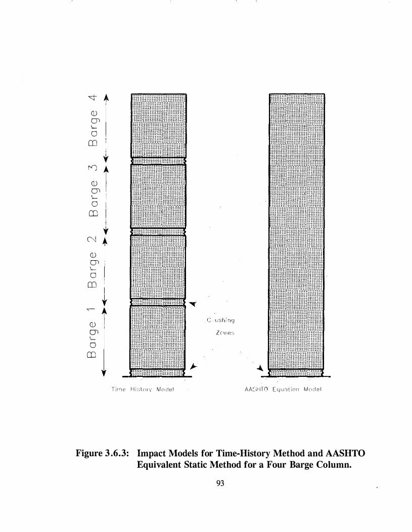
'<t A Q) 01 \.._ 0
m
t n t Q) 01 I \.._ I 0 I
m !
t (',!
Q) 01 \.._ 0
m
l .__- + Q) I ! 01 Zc1ne�'' \.._ 0
m
y T i n 1 e H i :;; t n rv M (_"l d e ! AA�lHT0 E q u n t i o n M n d e l
Figure 3 .6.3: Impact Models for Time-History Method and AASHTO Equivalent Static Method for a Four Barge Column.
93

--- - ------Legend
� B:u:go 1 (Lt!Ucl llurge)
� Bor�e2
"' D n"'�"·l
� B•rge4(Tmiliugllor�c)
---
"
171ps 13fps ' "" Impact Velooity
Figure 3.6.4: Barge Crushing Depths for a 35'x195' Barge Flotilla Column (four barges/column) .
94
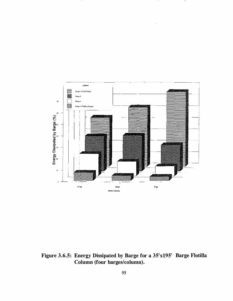
"'
Q) �511 "' <ll 1i' "'0 411
i -� Jll 0 e> Q) 2!1 " UJ
'"
Legend
� Burge 1 (LOilJ llur�c)
I§§ llargcl
D ll10rgc.l
� llarge 4 (Troiling Barge)
17fps
--- --- ��---·--------
13fps Impact Velocity
Figure 3.6.5: Energy Dissipated by Barge for a 35'x195' Barge Flotilla Column (four barges/column).
95
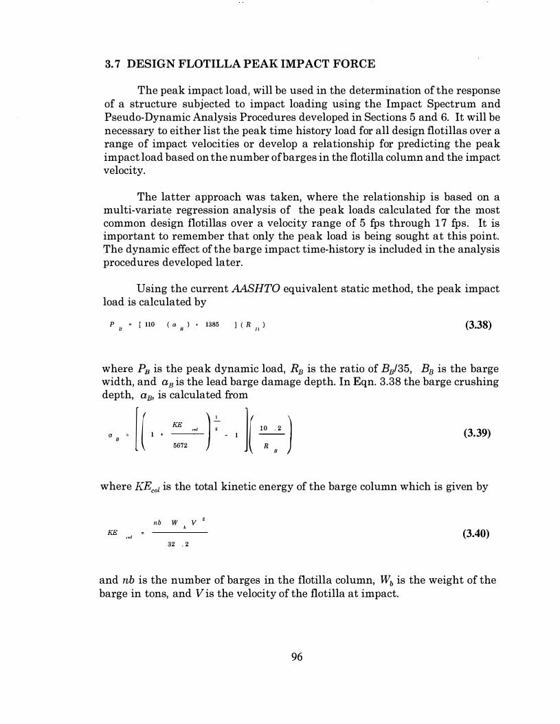
3. 7 DESIGN FLOTILLA PEAK IMPACT FORCE
The peak impact load, will be used in the determination of the response of a structure subjected to impact loading using the Impact Spectrum and Pseudo-Dynamic Analysis Procedures developed in Sections 5 and 6. It will be necessary to either list the peak time history load for all design flotillas over a range of impact velocities or develop a relationship for predicting the peak impact load based on the number of barges in the flotilla column and the impact velocity.
The latter approach was taken, where the relationship is based on a multi-variate regression analysis of the peak loads calculated for the most common design flotillas over a velocity range of 5 fps through 17 fps. It is important to remember that only the peak load is being sought at this point. The dynamic effect of the barge impact time-history is included in the analysis procedures developed later.
Using the current AASHTO equivalent static method, the peak impact load is calculated by
P 11 = ( 110 ( a 8 ) + 1385 ] ( R 11 ) (3.38)
where P8 is the peak dynamic load, R8 is the ratio of B8/35, B8 is the barge width, and a8 is the lead barge damage depth. In Eqn. 3.38 the barge crushing depth, a8, is calculated from
_ [ ( KE '"' ) � ]( 10 . 2 ) a n - 1 + - 1 --
5672 R n (3.39)
where KEcol is the total kinetic energy of the barge column which is given by
KE '"'
nb W V
32 . 2 (3.40)
and nb is the number of barges in the flotilla column, Wb is the weight of the barge in tons, and Vis the velocity of the flotilla at impact.
96
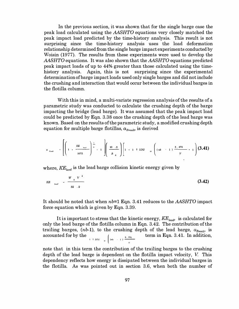
In the previous section, it was shown that for the single barge case the peak load calculated using the AASHTO equations very closely matched the peak impact load predicted by the time-history analysis. This result is not surprising since the time-history analysis uses the load deformation relationship determined from the single barge impact experiments conducted by Woisin (1977). The results from these experiments were used to develop the AASHTO equations. It was also shown that the AASHTO equations predicted peak impact loads of up to 44% greater than those calculated using the timehistory analysis. Again, this is not surprising since the experimental determination of barge impact loads used only single barges and did not include the crushing and interaction that would occur between the individual barges in the flotilla column.
With this in mind, a multi-variate regression analysis of the results of a parametric study was conducted to calculate the crushing depth of the barge impacting the bridge (lead barge). It was assumed that the peak impact load could be predicted by Eqn. 3.38 once the crushing depth of the lead barge was known. Based on the results of the parametric study, a modified crushing depth equation for multiple barge flotillas, a8,.,.u, is derived
a /lm.,/1 [ ( KE 1,.,.1 ) � ]( to 2 ) [ ( " I
5672 I --;;-:-- I • I 7 LOG '" ( nb
5 . 576 I )
v
where, KE1,ad is the lead barge collision kinetic energy given by
w v
• I ) (3,41)
KE ''"" (3,42) 32 . 2
It should be noted that when nb=l Eqn. 3.41 reduces to the AASHTO impact force equation which is given by Eqn. 3.39.
It is important to stress that the kinetic energy, KE1,ad• is calculated for only the lead barge of the flotilla column in Eqn. 3.42. The contribution of the trailing barges, (nb-1), to the crushing depth of the lead barge, aBmult• is accounted for by the
, , wu "' ( '"'' . I , � term in Eqn. 3.41. In addition,
v
note that in this term the contribution of the trailing barges to the crushing depth of the lead barge is dependent on the flotilla impact velocity, V. This dependency reflects how energy is dissipated between the individual barges in the flotilla. As was pointed out in section 3.6, when both the number of
97

barges/column and the impact velocity increases, so too does the energy dissipated in the barges other than the lead barge in the flotilla column.
The peak impact load is calculated using the AASHTO equivalent static load (Eqn.3.38), but is repeated here with the multiple barge flotilla peak load notation:
p " [ 110 ( a nmu/1 ) + 1385 (3.43)
where Pmax is the peak dynamic load, RB is the ratio of BB/35, and BE is the barge width. Figure 3.7.1 shows the peak impact load predicted by Eqn. 3.43 for a barge flotilla with 1-5 barges in the impact column and an impact velocity of 13 and 17 fps. This figure indicates that the design equation very closely predicts the peak impact load determined using the non-linear time-history analysis.
It should be noted that the design equation is slightly unconservative for the two barge column. However, for a two barge column with the theoretical maximum impact velocity of 17 fps the error is less than 4%, and for an impact velocity of 13 fps the error is less than 2%. Therefore, the upper bound of the error can be expected to be 4% and Eqn. 3.43 can be assumed to closely predict the time-history peak impact load. This allows for development of streamlined design procedures which will be given in Section 5 and Appendix_ III.
98

- - -- -
r-;:-:-:-:"'_, ________________ ,:-:-:-'-"'-':_;�;�'-'-"0-"'''-'-'-'-'"'-"--�-------'----------------"
-1
• Legend
Tlrr14-HIIWI"/V•17fpo
Number of Flotilla Column Barges
Figure 3.7. 1 : Peak Impact Load Comparison.
99

3.8 PIER IMPACT LOADING SPECTRUMS
The flotilla impact loading functions developed in section 3.5 are used to develop the pier impact loading spectrums in this section. An impact loading spectrum is analogous to an earthquake displacement response spectrum, with the exception that the loading is the result of mass excitation rather than base excitation. In order to. develop the impact spectrum of a single degree offreedom (SDOF) system subjected to a flotilla impact loading time-history, a starting pier stiffness and mass is assumed giving an undamped natural frequency, wP, and natural period, TP, of
w F ,, '
(3.44a)
2 n T (3.44b)
,, w "
where KP is the SDOF pier stiffness, and MP is the SDOF pier mass. The maximum displacement of the SDOF pier is determined over the impact loading history. The mass is incremented and the maximum displacement over the loading history is again determined. The mass is incremented n times such that all possible realistic natural frequencies for the structure are considered. The non -dimensionlized dynamic magnification factor, DMF, for the SDO F structure of natural frequency wP is calculated from
DMF (3.45) p
where, P,.ax I KP is the static displacement, v,<atio , I v(t) I max is the absolute value of the maximum displacement, and P,.=is the maximum load intensity over the impact loading duration given by Eqn. 3.43. The DMF is plotted versus the SDOF system period, TP, as shown in Figure 3.8. 1 . This will be discussed in greater detail later in this section.
The maximum response, I v(t) I max> of the SDOF freedom pier system of natural frequency WP and stiffness KP can be calculated by the solution of the convolution integral for damped vibration which is:
100

v ( t ) . ---[ M "' f, n,
p ( • ) e - � w ,, < t - < ) sin w ( t - 't" ) d "t" ] Ill' (3.46)
where, v(t) is the displacement at time t, p(r) is the loading function duration impulse, and UJnp is the damped natural frequency which is defined as
(3.47)
and, �= the ratio of damping to critical damping. Equation 3.46 is solved over
the time period 0 :-:;; 't' :-:;; t and the maximum response, I v(t) I max , is determined. Equation 3.46 is solved using the procedure given in Appendix II.
The application of the solution of the convolution integral in generating the impact response spectrums for a four barge column traveling at 13 and 17 fps and assuming a 5% damping ratio, results in the curves shown in Figure 3.8.1. As mentioned previously, the solution of the convolution integral uses the loading function derived for the case were the effect of pier flexibility on the loading time-history is ignored. The importance of ignoring the effect that the pier flexibility has on the impact spectrum will be explored in the next section.
3.8. 1 Effect of Bridge Pier Flexibility on the Impact Spectrums
One of the basic assumptions used in the derivation of the impact spectrums is that the effect ofthe bridge pier flexibility on the impact spectrums may be neglected. The effect of support displacement on the impact spectrum was investigated by application of the non-linear dynamic computer program given in section 3.6.
The maximum displacement for a pier of a given stiffness, KP' and mass, MP, was determined over the impact time history. The mass and/or the stiffness was incremented and the maximum displacement was determined at each step. This was repeated for a range of pier stiffnesses and masses resulting in a response spectrum surface. Cross sections of the surface are given in Figure 3.8.2 where each curve is for a pier of a specific stiffness.
The dynamic magnification factor is plotted against the undamped frequency rather than the period in order to clearly illustrate that neglecting the
101
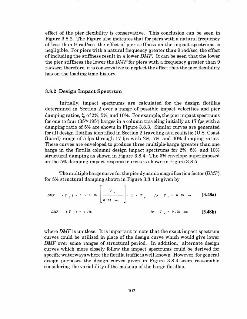
effect of the pier flexibility is conservative. This conclusion can be seen in Figure 3.8.2. The Figure also indicates that for piers with a natural frequency of less than 9 rad/sec, the effect of pier stiffness on the impact spectrums is negligible. For piers with a natural frequency greater than 9 rad/sec, the effect of including the stiffness result in a lower DMF. It can be seen that the lower the pier stiffness the lower the DMF for piers with a frequency greater than 9 rad/sec; therefore, it is conservative to neglect the effect that the pier flexibility has on the loading time history.
3.8.2 Design Impact Spectrum
Initially, impact spectrums are calculated for the design flotillas determined in Section 2 over a range of possible impact velocities and pier damping ratios, �. of2%, 5%, and 10%. For example, the pier impact spectrums for one to four (35'Xl95') barges in a column traveling initially at 17 fps with a damping ratio of 5% are shown in Figure 3.8.3. Similar curves are generated for all design flotillas identified in Section 2 traveling at a realistic (U.S. Coast Guard) range of 5 fps through 17 fps with 2%, 5%, and 10% damping ratios. These curves are enveloped to produce three multiple-barge (greater than one barge in the flotilla column) design impact spectrums for 2%, 5%, and 10% structural damping as shown in Figure 3.8.4. The 5% envelope superimposed on the 5% damping impact response curves is shown in Figure 3.8.5.
The multiple barge curve for the pier dynamic magnification factor (DMF) for 5% structural damping shown in Figure 3.8.4 is given by
DMF [ T " l , (3.48a) ( T ' ) I + 0 . 75 I ' T for T < 0 . 75 soc
/' /' 0 . 75 soc
DMF ( T " ) 1 . 75 for T p > 0 . 75 soc (3.48b)
where DMF is unitless. It is important to note that the exact impact spectrum curves could be utilized in place of the design curve which would give lower DMF over some ranges of structural period. In addition, alternate design curves which more closely follow the impact spectrums could be derived for specific waterways where the flotilla traffic is well known. However, for general design purposes the design curves given in Figure 3.8.4 seem reasonable considering the variability of the makeup of the barge flotillas.
102

No mention has been made up to this point about single-barge impact and design response curves. The results of this study indicate that an alternate curve is needed when designing for single barge impact. This is due to the fact that the higher frequency modes contribute more significantly to the impact response of the bridge pier. This can be seen in Figure 3.8.6 which shows the 5% envelope superimposed on the single barge 5% damping impact response curves. The proposed design curve envelopes for the 2%, 5%, and 10% structural damping are shown in Figure 3.8. 7.
The single-barge curve for the pier dynamic magnification factor (DMF') for 5% structural damping shown in Figure 3.8.6 is given by
DMF
DMF
( T P ) � 1 . 0 -r 0 . 4 [�j 0 . 20
< T ,. ) • 1 . 4 • . 35 [ T , · 0 . 2 ]
3 . 05
DMF ( T /' ) = 1 . 75
for T P :;. 0 . 20 sec (3.49a)
for 0 . 2 see < T � 3 . 25 sec ,.
(3.49b)
for T 1, :> 3 . 25 sec
where the DMFis unitless. The procedure for utilizing the preceding curves to generate a design loading will be given in the next Section where the modified impact design equations are developed.
A very important point about the dynamic response of bridges to barge impacts can be deduced from the design spectrum given in Figure 3. 7 .4. From the figure it can be seen that for barge impact the DMF increases up to a period of approximately one second, after which .the DMF remains constant. This is in direct contrast with the behavior of bridges to the other common dynamic excitation, namely earthquakes. The Standard Specifications for Highway Bridges, Division I-A, Section 3.2, gives an idealized spectrum which shows that the structure earthquake response increases until a period of approximately one second reached and then decreases to a DMF of 0.4 at three seconds structure period.
This is important from a design standpoint since for earthquake dynamic design, increased structure period is desired in order to reduce the maximum overall structure response. However, for barge impact it seems that increased structure period will not reduce the structure impact forces. This implies that earthquake techniques such as dynamic isolation, and plastic design will not be beneficial for reducing impact member design loads.
103
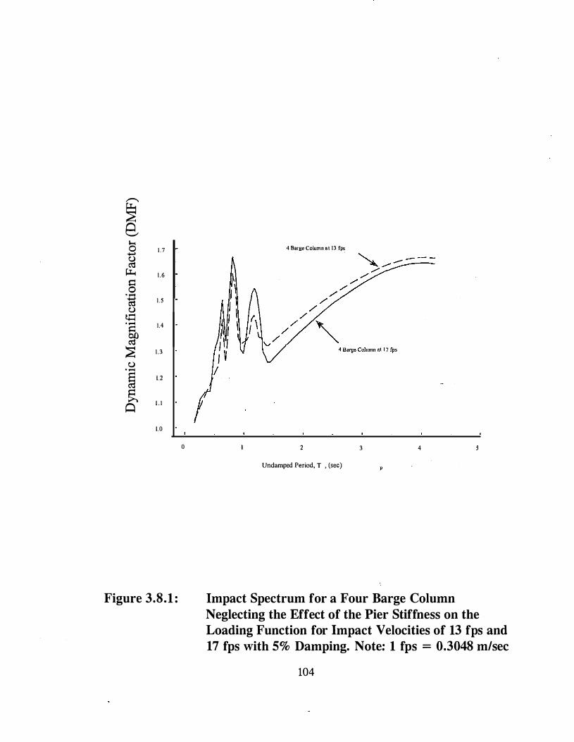
,.-., � B ..... 0 1.7
� � 1.6
1::1 0 . .... ttl 1.5
u t;:1 . .... � 1.4
� 1.3
u . ....
g 1.2
� 1 . 1 Q 1.0
Figure 3.8.1 :
v
0
4 Barge Column at 13 fps
2 3 4
Undamped Period, T , (sec)
Impact Spectrum for a Four Barge Column Neglecting the Effect of the Pier Stiffness on the Loading Function for Impact Velocities of 13 fps and 17 fps with 5% Damping. Note: 1 fps = 0.3048 m/sec
104

/'""'-� 2
1 .9 '-'
El 1 .8
� 1.7 � 1=1 0 1 .6 . ..... � t3 1 .5
"§1 1 .4
� 1.3 <.) . .....
g 1 .2
s 1 . 1
0
· · · · · · · · · · · · · · · · · · · · · · · · · · <"9 fadis'eC • · · · · · · · ·I· · · · · ;,:g: ia'd/SeC · · • · · · · · · · · · · · · · · · · · · · · · · · ·
-<--- I ,.. · · · · · · · · · · · · · · · · · · · · · · · · ·r · · · · · · · · · · · · · · · · · · · · · · · · · · · · · · · ·
I highest stiffness · · · · · · · · · · · · ·} ·
·
· · · · ·
..
· · · · · ·
.
· · · · · · · · · ·\ I
· · · · • · · · · · · ·
I · · · · · · · · · · · · · · ·��·
"·
'.:..:.
· · · · · · · · · · · · · · · · · · · · · · · · · · · · · · · · T · · · · · · · · .
· · · · · · · · · · · · · · · · · · · · · · · · · · · . . . . . . . . . . . . ! . . . . . . . . . . . . .
I . . . . . . . . . . . . ·I· . . . . . . !��� �t!f!��s� . . . . .
I
K
· · · · · · · · · · · · · · · ·r · · · · · · · · . . . . . . . . . . . . . . . . . . · · · · · · · · · · ·
5 10 IS
ro r (rad/sec)
"'
20
Figure 3.8.2: Influence of Pier Flexibility on the Impact Spectrum for a Single 35'x195' Barge.
105
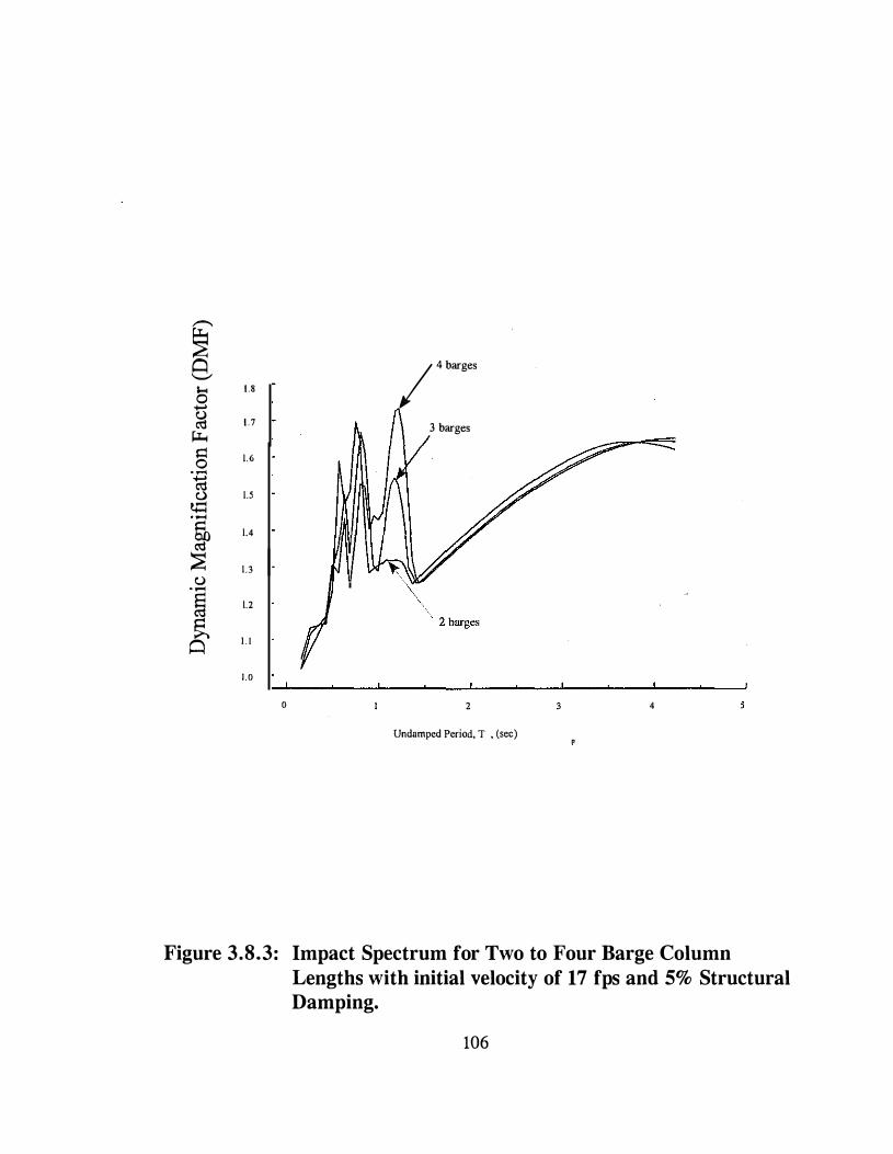
""""' � 8 /4barges ..... 1.8 0
� 1.7 3 barges �
§ 1.6 . ..... � c.> 1.5 t+=1 ...... � 1.4
� 1.3 u . .....
§ 1.2
� 1 . 1 0 1 .0
0 2 4
Undamped Period, T , (sec)
Figure 3.8.3: Impact Spectrum for Two to Four Barge Column Lengths with initial velocity of 17 fps and 5% Structural Damping.
106

� �
Maximum DMF= 1.85 @ 2% Damping
...... 1 . 8 0 t) 1.7 «! Maximum DMF= 1.75@ 5% Damping
>"-i � 1.6 0
·.p «! 1 . 5 � Maximum DMF"' \.60@ 10% Damping
-� 1.4
� 1.3 u
. .....
� 1.2
s 1 . 1
1.0
0 .5 .75 1 .0 1 .5 2.0 2.5
Undamped Period, T � , (sec)
Figure 3 .8.4: Proposed Multiple Barge Design Impact Spectrums for 2%, 5% and 10% Structural Damping.
107

,......_ � Ci '-' ..... �
� � 0
· -
"t;:j C)
� . .... � � C) · -
§ � Ci
1.8
1 .7
1.6
1.5
1.4
1.3
1.2
1. 1
1.0
0
� I ,! I ) I f I
!J ' I ,V I
I
I Do.ign Cu<"<
2 3 4
Undamped Period, T P , (sec)
Figure 3.8.5: Multiple Barge 5% Design Curve Superimposed on 5% Damping Response Curves.
108
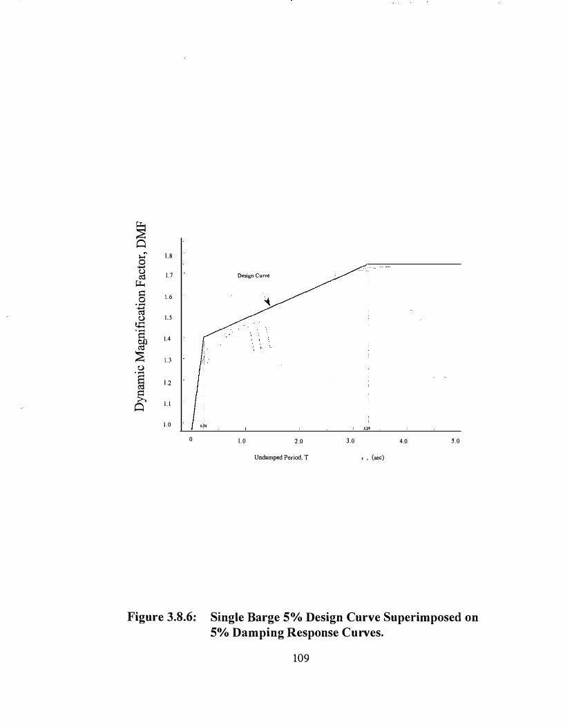
� �
..... 1 .8 0 t) 1.7 ro Design Curve
� !:I 1.6 0
· -
'iii u 1.5
� · -� 1.4 \ '; \
;;2 l .3 I u · -
§ 1 .2
� 1 . 1 � 1 .0 lllll J.l�
0 1.0 2'.0 3.0 4.0 5.0
Undamped Period, T , • (sec)
Figure 3.8.6: Single Barge 5% Design Curve Superimposed on 5% Damping Response Curves.
109
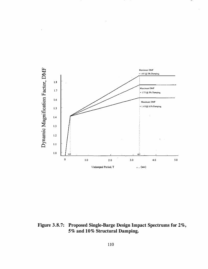
� Maximum DMF = 1.85 @ 2% Damping
0 ..... 1.8 0 t) ; Maximum DMF c;l 1 .7
� )= 1.75 @ 5% Damping
1::1 1.6 0 . ..... Maximum DMF
1ij 1.5 : ._ ! .65@ 1 0 % Damping
u t$:1 ·� ro
1.4
� 1 .3 u . ..... § 1.2
� 1 . 1 0 1.0 11.2!1 3.��
0 1.0 2.0 3.0 4.0 5.0
Undamped Period, T � , (sec)
Figure 3 .8.7: Proposed Single-Barge Design Impact Spectrums for 2%, 5% and 10% Structural Damping.
1 10

3.9 CONCLUSIONS
This Section developed the impact load time histories for the design barge flotillas developed in Section 2. The results of this Section showed a significant difference between the peak impact loads predicted by the time-histories and the peak loads predicted by the current AASHTO impact load analysis method. The greater the number of barges in the flotilla column the greater is the difference between the time-history results and the AASHTO equations. The AASHTO equations are based on the results of single barge impact test results. The difference seems reasonable since the AASHTO method neglects the interaction between the individual barges in the flotilla column.
Within this Section, a non-dimensionalized design impact spectrum was presented. The spectrum was developed by plotting the individual nondimensionalized impact spectrums for the design flotillas with initial velocities of 5 fps through 17 fps on a single plot and then enveloping the composite plot. It was shown that the effect of pier flexibility on the impact spectrums could be conservatively neglected for design purposes. The following Section will utilize the design impact spectrum as part of two proposed dynamic analysis procedures that include the dynamic effect of the impact loading on the development of the bridge design loads.
It was shown in this Section that increased structure period does not decrease the dynamic response of the bridge to barge impact. This is contrary to typical dynamic seismic design, where after a structure period of one second is reached further increases in the structure period reduce the dynamic response ofthe structure to earthquake excitation. Therefore, for impact design, isolation or plastic behavior would seem to have no benefit in reducing the peak structure design forces.
1 1 1
4.0 IMPACT MODAL RESPONSE EQUATIONS
4.1 INTRODUCTION
The purpose of this Section is to derive the impact modal equations to be used in the Pseudo-Dynamic and Impact Spectrum Analysis Procedures developed in Sections 5 and 6, respectively. The basic approach for the design procedures is to combine the predominate inertial modal response, determined from the impact spectrums derived in Section 3, with the pseudo-static response. The inertial mode response is determined by using assumed normalized mode shapes, rather than by eigenvector or Ritz-vector solution. This approach is used as a means to eliminate the need for computer solution ofthe eigenvector or load dependent Ritz-vectors.
The following sections develop the modal impact equations which will be used for derivation of the Pseudo-Dynamic Analysis Procedure (PDAP) and the Impact Spectrum Analysis Procedure (ISAP). Development ofthe modal impact response equations is accomplished by: 1) the modal response equations, and 2) the pseudo-static response equations.
4.2 Modal Response Equations
The response of a structure may be determined using a modal impact spectrum analysis similar to the procedures used in earthquake analysis. However, several differences exist that do not allow currently available engineering software to be used for determination of other than the modal frequencies and mode shape vectors. These differences will be discussed in detail later in this section after the development of the modal response equations.
In order to determine the overall response of a structure using an impact spectrum analysis, the dynamic contributions from the individual modes are considered. Using the orthogonality properties of the individual modes, n, the n'" mode displacement component, u,, is given by the product ofthe mode-shape vector, Q:>,., and the modal amplitude, Y"' where the total response is expressed by
N
{ v } L { <I> } y (4.1)
1 12
where N is the total number of included modes. In matrix notation Eqn. 4.1 is written
{ v } 0 [ <I> l { y } (4.2)
where [<l>] is the NxN mode-shape matrix which transforms the generalized coordinate, Y, to the geometric coordinate vector {v}. To evaluate any arbitrary normal coordinate, Y," Eqn. 4.2 is multiplied by , • 1 ' l to obtain
' ' ( !!J l , [ m ] { u } = { !jl l ., [ m ] { l(l } 1 Y 1 + { <fl ) T [ m ] { tfl } Y + • • • + { <) } 7' [ m ] { !jl } Y 10 2 2 II N ,\' (4.3)
Because of the orthogonality property with respect to the mass matrix, m, all terms on the right-hand side of the equation are zero except for the terms
1" containing { 4> 1 . [ "' 1 { 4> 1 • This gives
T { 4> 1 , [ m ] { v l
y (4.4) '/"
{ 4> I [ "' l 1 4> I
If {v} is time dependent then Y,, is also time dependent; therefore, taking the derivative of Eqn. 4.4 with respect to time gives
1' 1 4> I [ m ] l v' ( t ) l
y ( \ ) (4.5) T
I 4> I [ "' l 1 4> I
Using the results given by Eqns. 4.4 and 4.5, it is possible to write the equation of motion of the multiple degree-of-freedom system (MDOF) in terms of the generalized coordinate vector Y. The damped equation of motion for the MDOF system written in terms ofthe acceleration, ,, ' " , damping matrix, [c], stiffness matrix, [k] , and load time-history, {p(t)}
[ m I I ,. ( t ) I • [ , I I v· ! t ) I • [ k I I v ( t ) I o IP ( t ) } (4.6)
Taking the second time derivative ofEqn. 4.4 and substituting these results and Eqns. 4.4 and 4.5 into Eqn. 4.6 gives
1 13

(4.7) " o I
Multiplying by the m'" mode-shape vector ' } g1ves
T T { � } [ m ] l � l . I Y ( t ) } • { � } [ o ] { $ l
,I Y ( t ) } •
T T (4.8)
{ � } [ h ] { $ } { Y ( l ) } { $ } { p ( l ) }
However, by the orthogonality conditions
1' { � } [ h J { $ } " 0 foe "' ' "
.,. { ·� } { m J { $ } " 0 for "' ' n (4.9)
T { <{> } [ ' J { <{> } " 0 for "' ' n
If the symbols T
p I t ) • I � l { p ( t ) l (4.10a) " .,. (4.10b)
M { � l [ m J { � l (4.10c)
.,. (4.10d) c { � l [ ' J { � l
1' K { � l [ k J { � l
are introduced, Eqns. 4.10 represent the modal load, P,(t), modal mass, M.,, modal damping, C., , and modal stiffness, K,,, respectively. Eqn. 4.8 can then be written as
M Y ( t ) • C Y ( I ) • K Y ( t ) P ( t ) (4.11)
Eqn. 4. 11 can be expressed as
y ( t ) + 2 � w y ( t ) + (J) y ( t ) p " ( t )
(4.12) M
1 14
where the modal viscous damping ratio, "' , is defined as
and
w
c
2 w M "
K
M
(4.13)
(4.14)
The modal load, P,.(t), in the right-hand side ofEqn. 4.12 can be expressed as
p ( I ) 'I' T
I � I I P I I ) I e I � I I R I f ( 1 ) (4.15)
where {R} is a load magnitude distribution vector and f(t) is a force amplitude function of time. Substituting Eqns. 4.15 and 4.10a into Eqn. 4.12 gives
y " ( I ) '
2 ( w Y ( I ) • w Y ( I ) e ll " II " (4.16) ,.
I � } " [ m ] { � }
Since earthquake loading is the dynamic loading type for which most civil engineering software has been developed, it is important to point out the unique aspects of impact spectrum analysis as compared to response (earthquake) spectrum analysis. This comparison will highlight why response spectrum software cannot be used for impact spectrum analysis.
For the special case of earthquake loading, the time varying load vector, {P(t)}, first presented in Eqn. 4. 7 is expressed as 1 , , , , , • 1 "' 1 1 11 , ,, , inwhich 1 •
is the earthquake acceleration history applied at the structure supports and {Req} is a displacement transformation vector that relates the displacement of each structure degree of freedom to the static application of a support displacement. When spatial variations in the base are neglected, {Req} is a unit column vector.
1 15
For impact problems, the time varying load vector, {p(t)}, is expressed as 1 , , , , 1 � 1 u 1 " , , , and {R } would be zero for all structural degrees-offreedom except those associated with the external load vector, {p(t)}. Therefore, the load vector cannot be expressed as the product of the mass matrix (Eqn. 4.15) as is the case for the earthquake loading. This indicates that currently available commercial codes for earthquake response spectrum analysis cannot be used for impact spectrum analysis without modification of the code for the specific aspects of impact analysis.
The ratio on the right-hand side of Eqn. 4.15 defines the modal participation factor, rn , for mode n and is written
T { � I , I R I
r 1'
(4.17) I � I , l m I { � I
which can be physically interpreted as the overall contribution of a particular mode to the dynamic response of a structure. To proceed with the solution of the impact spectrum response, the convolution integral (Eqn. 3.46) can be expressed
y " I t ) , M
- � " w " ( I - t ) P ( 't" ) e sin w D" (4.18)
as the modal equivalent for the n'" mode of natural frequency, wn, where, P,.(r) is the mode loading function duration impulse, and WDn is the damped mode natural frequency which is defined as
(4.19)
and, �=the ratio of the mode damping to critical damping. Equation 4.18 is solved over the time period 0 ,; 't':> t and the maximum response, I Y,,(t) l max , is determined; therefore, Eqn. 4.18 is written
� "' ( I I Y i t i I
1 16
, , ] sin w ( t - • ) d • "" · max
(4.20)

Since the impact spectrums are derived from the solution of the convolution integral for the SDOF case, application of the impact spectrums to the MDOF case requires only rewriting Eqn. 3.39 (developed in Section 3) to its modal equivalent of
DMF ( ( , w )
where
w " " F. '
M "
K , I Y ,. { t ) i m"� (4.21)
p
(4.22)
and modal damping, �" , is defined in Eqn. 4.13. Therefore, the maximum modal displacement is written
DMF
I Y ( t ) I mn� (4.23) K
Equation 4.23 gives the modal maximum response in terms of the dynamic magnification factor determined from the impact spectrum derived in Section 3. This equation can be utilized to determine the impact structural response after determining the modal frequencies and shapes. This is directly analogous to seismic design response spectrum analysis. However, the intent of this Section is to develop simple, modified design equations where eigenvector analysis is· not necessary. The key to accomplishing this goal, which is detailed in the next section, is to develop the equations whereby the dynamic singlemode response can be combined with the pseudo-static response to give the total structural impact response.
4.3 TOTAL MODAL DYNAMIC RESPONSE
It will be shown in this section that the total modal dynamic response can be resolved into those modes for which the inertial effects are significant and those modes for which the inertial effects may be neglected. The modal response for which the inertial effects may be neglected will be referred to as the pseudo-
1 17
static response. Those modes for which the loading history of the loading are significant will be called the inertial modes.
In order to develop the total response equations, the dynamic structural response is resolved into the contribution oflower modes and higher modes. It was shown (Lager, and Wilson, 1988) that if the temporal distribution of the forcing function is such that the higher modes of the system are significantly excited, these modes must be included. However, if the higher mode frequency is much larger than the highest frequency content of the applied loading, the response in the higher mode is essentially static. The applicability of the latter conclusion to barge impact problems is evident from the impact spectrums developed in Section 3.
Plotting the dynamic magnification factor (DEF) of the design response spectrum curves (given in Section 3.7) versus the frequency (rather than the period, as was done in Section 3) gives the frequency response curves for 2%, 5%, and 10% damping as shown in Figure 4.3.1. From the curve it can be seen that as the mode frequency increases the DMF approaches unity. This is true even for relatively low structure mode frequencies of 25 radian/second. Therefore, it is reasonable to conclude that the inertial effects of the higher modes may be neglected and their response can be calculated by simple static analysis. Thus, the mode superposition equation which is given by
(4.24) " � I
can be written as
N
{ o ( t ) } L { � } Y ( t ) { � } y ( t ) " · ''
(4.25) " = rl ' I
where the summation of n from 1 to d represents the number of modes with significant inertial effects, and n from d+ 1 to N represents the response where the inertial effects are negligible, i.e., the pseudo-static response. The response for the first d modes can be calculated using the solution to the eigenproblem, etc. and the response due to the remaining modes can be calculated by static analysis. Therefore, the mode pseudo-static response, < ' l , for mode n is
1 1 8

y ( t ) S , IJ
K
T � � I " IP ( t ) l
( n ?. d + l ) T
I � I l k I I � I
The pseudo-static displacement for mode n can then be written as
I " I t ) I I � I Y ( t ) I � I p " ( l )
K
(4.26)
(4.27)
The summation of the pseudo-static responses for the high modes for which the inertial effects may be neglected, {v,H(t)}, is
I " I t J l ""
.v
I " I I t J
N
I � l Y I t J " . . "
The total response, dynamic plus pseudo-static, is then
1 " 1 ' n I: 1 � 1 Y < t >
" = l
N
I � I Y I t ) " " · "
(4.28)
(4.29)
In the current form, Eqn. 4.29 still requires the evaluation of the higher modes in order to calculate the total modal response. However, the total pseudo-static structural response for all modes, {v(t)},,"'''' is
l " ( t ) l " [ k ] - I R l f ( t ) M<lli<" (4.30)
The pseudo-static response for the first d modes is then subtracted from Eqn. 4. 30 to give the pseudo-static response of the high modes ( modes d+ 1 to N) , which is expressed by
,,
- ' l v ( t ) l " [ k ] I R } f ( t ) .. u " " l
{ � } Y ( t ) . "
1 19
(4.31)
It is important to note that Eqn. 4.31 represents the pseudo-static response of the high modes and only the first d modes need to be calculated. Substituting Eqn. 4.31 into Eqn. 4.29 gives the total dynamic response, {u(t)},
,,
" ' I
( q, " l y ( ' )
,, (4.32)
" � I
in which the first term is the dynamic response of the first d modes (inertial plus pseudo-static), the second term is the pseudo-static response of the first d modes, and the third term is the pseudo-static response of all modes due to the loading time-history vector {p(t)}.
In order to utilize the impact spectrums, developed in Section 3, Y,Jt) from Eqn. 4.20 is substituted into the first term of Eqn. 4.31 to give the following
,, DMF p ( " ( ! ) } 0 I: ( <J> l L ( <!> } " -"
• [ k ] - 1 ( R } f ( t ) (4.32) " = 1 K " ' I K
Equation 4.32 represents the impact response due to all modes where only the eigenvalues and eigenvectors for the lower modes are calculated since the inertial effects of the higher modes are neglected. This equation will be utilized in Sections 5 and 6 to develop the Pseudo-Dynamic and Impact Spectrum Response Methods, respectively.
120

Maximum DMF = 1.85 @ 2% Damping
1 . 8 Maximum DMF = 1.75
1 . 7 @5%Damping
Maximum DMF = 1.60
1 . 6 @10% Damping
1 . 5
1.4
1 . 3
l . 2
1 . 1
1 . 0 "'"""""'""'""""""""'"'"""""""""""""".:"""""""""""""'""""""'"""""""""'"'"'""""""'"'"'"'"'""""""""'"''"
0 5 7.0 1 5 20 25
Undamped Frequency, ro , {rad/sec)
Figure 4.3. 1 : Frequency Response Curve for 2%, 5% and 10% Structural Damping.
121

4.4 CONCLUSIONS
The modal response equations required to develop the Pseudo-Dynamic and Impact Spectrum Analysis Methods (PDAP, and ISAP) were derived in this Section. The derived equations show that the impact response of a structure may be calculated using only the lower mode response. This response is determined from the impact spectrums derived in Section 3, and the static response to the peak (maximum) of the barge impact loading time history. This result is significant since the higher mode response can contribute significantly to impact problems.
In the following Sections, the PDAP and ISAP will be developed whereby the impact response of the structure is determined without computer solution of the lower eigenvectors. The procedures given provide the bridge designer a rational method for evaluating member design forces, and yet is not analytically cumbersome.
122

5.0 PSEUDO STATIC ANALYSIS PROCEDURE (SINGLE INERTIAL MODE PROCEDURE)
5.1 INTRODUCTION
The purpose of this Section is to propose modifications to the current AASHTO Guide Specification equivalent static design procedure by including the dynamic effects of the barge/pier collision. The procedure used here is an impact spectrum single-mode design procedure which is called the PseudoDynamic Analysis Procedure (PDAP). The basic approach for the proposed design procedure is to combine the predominate single-mode dynamic effect response, determined from the impact spectrums derived in Section 3, with the pseudo-static response. The actual single-mode response is determined using an assumed generalized mode shape approach, rather than by eigenvalue solution.
One of the most attractive aspects of the current equivalent static design methodology is its simplicity of integration into the design process. In order for a new revised design methodology to be of practical benefit, it should follow in the same form of the current AASHTO equivalent static design methodologies. Therefore, the suggested revisions to the current code will be presented in the form of design formulas, and graphs that are easily applicable to the "typical" barge impact bridge design problem.
The revised design procedure uses the previously derived barge impact loading spectrums which are based on the experimentally derived barge loaddeformation relationship. Using the impact loading functions, a nondimensional design impact spectrum was developed. From the impact spectrum, the modal impact forces for a bridge pier will be determined depending on the dynamic characteristics of the structure.
The results of the maximum response, determined using the modified design procedure, are compared to the response determined using the current AASHTO equivalent static method and a linear dynamic time-history analysis [which is called the Time History Analysis Procedure (THAP) herein] using the barge impact loading time-histories developed in Section 3.
5.2 BRIDGE DESIGN PROCESS
Prior to the development of the PDAP, it is important to remember that the PDAP is only a part of the overall bridge design process. The AASHTO Guide Specification gives three statistical design procedures called Method I, Method II,
123

and Method III as was shown in detail in Section 2. Therefore the PDAP must be integrated into the overall design method. Figures 5.2.1 through 5.2.4 provide a detailed flow chart of the integration of the PDAP in the chosen statistical design method.
124

_y__
AAS/ffiJ
Figure 5.2.1 : Suggested Design Procedure Flow Chart.
125
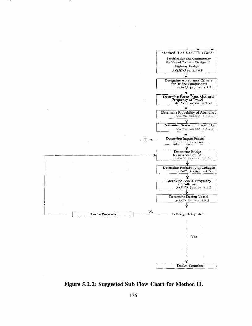
Method II of AASHTO Guide Specification and Commentary
I for Vessel Collision Design of
'I Highway Bridges AASHTO Section 4.8 !
== =t - =- = I Determine Acceptance Criteria ! for Bridge Components i
_, __ _ ___ _ _ __ AASH_Tc_Ser�inn +.8.:f_ __ _j y l - oete���j �!�����r::d _ ]
- --- - - . - ---"" ----''
-----
--
! Determine Probability of Abenancy! L_ AASHTn Se<ccinn 4 . R . .3.�_j - · -- ' -----:1 · · - --·· ···-
'\" [' nt!termfrie Ge01.J�etric PrObabilliYl AA5hTO Section 4.R.3.3 ! - -- ·--:r- - - --- -'
'\( -- DE:te�e ImpaCt
-FOr�e�-,-, I ...C:-- ':'J"t��____:;��fli:�"':'_'�:,r - ' I ;
____ __ y _ __ - ---· ·
�- -- --· ----- ---- ---- -· · -- - ··-· ··- -1_ Determine Bridge Resistance Strength AASHTn Sectinn 4.8.3.4 _j -----1 ' --- . ---I
L ---- r
----
-----Revis;Sh-uctur�-------
� - '] -- · No
,------ --- -----�- ----------------1 Determine Probability of Collapse : \_
------ --�A-�SIHD _:se:.�-�-i�i�. -.::-R.:1 . 4 __ _j [--Det�rmm.e �ual Ffequ�ncy
of Collapse . A"? SI-ITO S_ection_ 4.8.3 _ _ _I
==--- {. =-- -=-I Determine Design Vessel L_ AASHTO SP.dinn 4.8.2
f'-Is Bridge Adequate?
Yes
� L_
:l Design Complete
Figure 5.2.2: Suggested Sub Flow Chart for Method II.
126
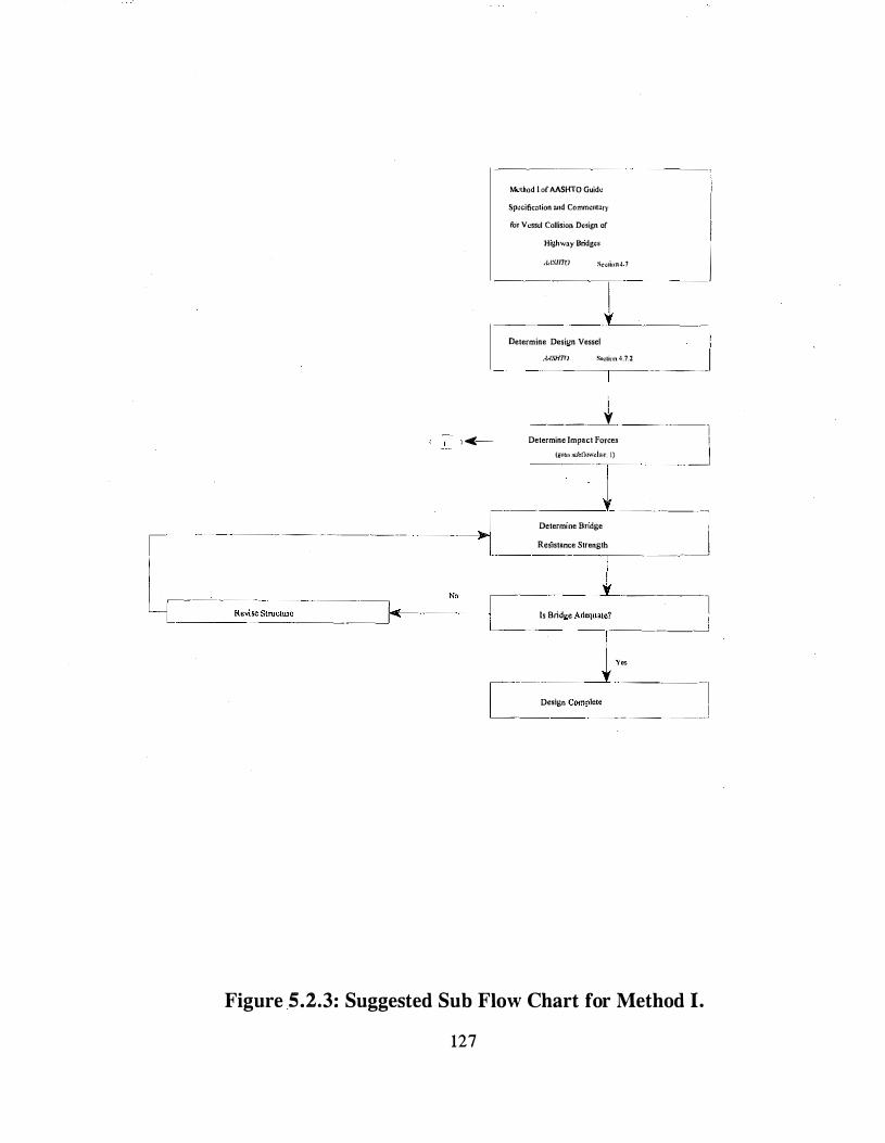
t <(-
Method 1 of AASHTO Guid�
Sp�cifkntion and Commcnt:lry
fbi" Vessel Collision Design of
H1ghway Bndg�s I AA:>ii1V �,�IIC>n4 7 -- � ---1 Determine Design Vessel AASHT() Soclitm4.7.2 --J
1---�___I __ _ --1 _j Determine Impact Forces
(gC>�l •ubtlowclmrt l)
�� -� - -'! _ _
_ { Determme Bndge 1 � -���- -------- ----- Res1stance Strength --���
Lc- R"i"Stru""'' -=--�- ---
N°
--I --- .. ., . . _.� -- l _' J-v.. _ __ _j
[- D'"igo Comp...._ =--�I
Figure .5.2.3: Suggested Sub Flow Chart for Method I.
127
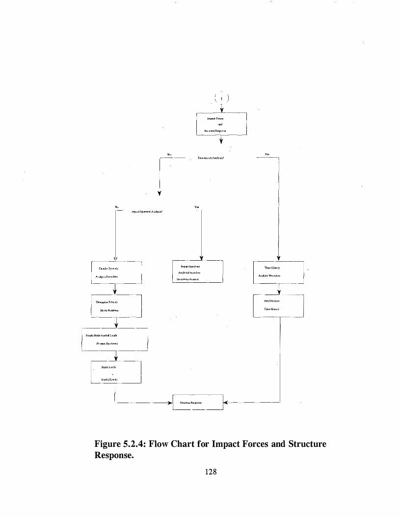
No h .�····- Tomo-ki"'OI}'ilooi)�W
y
l-::.:,-;:.:! --J 1\.,uly.<i•l'moo<lurc
"'""'""��,.,.,,...,,) --����- [----::;.:----], -A,,�,.;, Pr<,._�ou., .. � 1 -
[_______':f_J_ A��lyl"'l"'"
Timo·llt<lu<)'
-r Figure 5.2.4: Flow Chart for Impact Forces and Structure Response.
128
5.3 PSEUDO-DYNAMIC ANALYSIS PROCEDURE (PDAP)
It was shown in Section 4 that the total modal response could be resolved into those modes for which the inertial effects are significant and those modes for which the inertial effects may be neglected. For the derivation of the pseudodynamic analysis procedure, it is assumed that the dynamic effects for only a single mode need to be considered. Hence, Eqn. 4.28 is written for the maximum response over time (f(t)=l.O) as
{ v } DMF ( ( , <u ) P P
o { � l -----'--'-'--'-- • I � l - • [ k I - ' { R I K K
(5.1)
and assuming that d=l and the term, [k] ·'{R}, is the total static response of all modes. Therefore, Eqn. 5 .1 is written such the total response, {v},ax• is determined in part by modal analysis and in part by ordinary static analysis which is written
{ " l (5.2)
where (f(t)=l.O)
DMF « ' "' ) p p (5.3a) { " l marin/ � � l { � } -/( /(
{ " l I k I - ' { R l (5.3b)
Blfllio·
In order to solve Eqn. 5.3a, the determination of the inertial mode shape is required. When a bridge pier geometry is such that a single inertial mode may be assumed, calculation ofthe mode shape using the solution of the eigenproblem can be avoided. This is accomplished by assuming that the displacement for the pier system can be generalized as a distributed SDOF system. The differential equation of motion for the generalized undamped SDOF system is rewritten as
M y' ( t ) • K . Y ( l ) o P . ( t )
where the generalized mass, M, and stiffness, I(, are given by
129
(5.4)

'
M J "' '
( x ) [ W ( x ) ] dx . E ' (5.5a)
"' l W ( X ,J I
(5.5b) . K J k ( X ) [ $
" ' ( x ) ] dx • E k [ w
" ( X , l l '
nd m(x) is the mass distribution function, mi is the i'h lumped mass, k(x) is the stiffness distribution function, ki is the i'h lumped stiffness, lji" (x) is the second derivative of the assumed mode displacement function (which will be discussed in detail in the following paragraphs), and lji"(x;) is the mode displacement function second derivative evaluated at the x coordinate of the i'h mass or stiffness. p•(t) is the generalized load which is expressed as
/, P · ( t ) • J p ( x , t ) � ( x ) dx • L p 1( t ) � ;< x ) " (5.6)
where p(x,t) is the spatial and time varying loading function, and pJt) is the i'h time varying concentrated load.
The generalized first mode natural frequency, CUg, can be written in terms of the generalized stiffness, K*, and generalized mass, M *, as
(5.7) '
In order to utilize the equations developed in Section 4, it is necessary to convert the discrete modal equations into generalized coordinate equations. By analogy, Eqn. 4.25 for the maximum (over the displacement time-history) generalized continuous displacement function, Y,.ax• is written
y '
! "
/,
! " p ( x ) � ( x ) dx
II 2 k ( x ) [ W ( x ) ] dx
.
•
E
E
P 1 W ( x 1 )
II 2 k . [ $ ( x ) ] ' '
130
p (5.8)
K
Therefore, the continuous generalized mode response, v(x)madal which is analogous to Eqn. 4.25 for discrete modal displacement, is written as
p 'i> ( X ) y <I> ( x ) -- (5.9)
K
Based on the results of the preceding discussion Eqn. 5.2 can is rewritten for a distributed parameter system as
V ( X ) 11wd•tl
DMF ( ( . w ) P
<I> ( x , l -----''-- p <I> ( x
.) --
K K
Simplifying gives the maximum modal response which is written
V ( X ) mmlu/
[ DMF ( ( , w ) - l ] P g <I> ( x ) -----�----
K
(5.10)
(5.11)
In Eqn. 5.2, the modal response,u(x),.odal> is added to the static response,u(x),,01;,, to produce the total impact response, v(x),nax·- For design purposes, the way to combine the two responses is to first determine the distributed structure forces resulting from the modal displacement, v(x)madal (Eqn. 5.11) and second, to apply these forces simultaneously with the static impact force, Pmax> which is given by Eqn. 3.43.
The inertial forces, fr(x) produced by the distributed modal displacement, v(x),.odal> are given by (e.g., Clough, and Penzien, 1993)
- w m ( x ) v ( x ) I! morl«l (5.12)
and for the i'h concentrated mass the concentrated inertial load is simply
- w m g V ( X ) i "'"rl"/ (5.13)
Since the inertial force direction reverses direction over the displacement time history, the negative signs in equations 5.12 and 5.13 will be neglected from the
131

notation from this point on. The effect of the inertial force reversal will be considered later in the form of load cases in the design example problem. The static and inertial loads are shown in Figure 5.3.2 without regard to direction.
In order to apply the simplified design method, a single mode displacement function must be assumed. For impact problems on cantilever bridge piers, the shape can be reasonably expected to be of the cubic form (Figure 5.2.2), whereljJ(x;) is written as
(5.14)
Equation 5.14 satisfies the boundry conditions, ljJ(O)=O, ljJ' (0)=0, ljJ' (L)=O, assumed to model the displaced shape. Substituting Eqn. 5.14 into Eqns. 5.6 and integrating gives the generalized first mode system properties. For the structure shown in Figure 5.2.1 where the columns of the pier are identical, the generalized stiffness I( is
12 E I K n (5.15)
L
where E is the elastic modulus, L is the column length, and n, is the number of columns. The generalized first mode mass, M, is
13 M - m
35 , , L n + m L c· l ,. <' I' <' I' (5.16)
where mo� is the distributed mass of the columns, Lo� is the column lengths, m,P is the distributed mass of the pier cap or concentrated mass at the column top, and L,P is the length of the pier cap or concentrated mass at the column top. Other assumed displacement shapes for different pier configurations can be used to derive similar results.
132

P(t)
f (x) = OJ m v{£) I
+ p
Figure 5.3 .1 : Equivalent Response Using Psuedo-Dynamic Analysis.
133
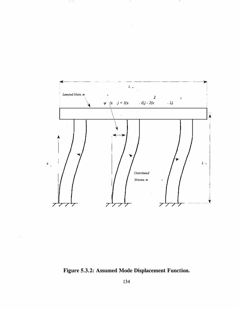
X
· -· ··--- -----·-----·---
Lumped Mass, m '
\ �
L .,
1J1 (x ,) = 3(x I
2 , IL) - 2(x
Distributed Masses, m
· -- --->c
' L}
L ' I
I y
Figure 5.3.2: Assumed Mode Displacement Function.
134

5.4 STEP-BY-STEP PDAP
The results given in this Section have resulted in a simplified barge impact analysis procedure whereby the dynamic effects of the interaction of the individual barges in the flotilla and the bridge are included. However, actual application of the preceding results to an analysis problem have not been presented. Therefore, this section presents the preceding results in a step-by-step format which will be explicitly followed in the following section in the form of a design example.
The procedure to calculate the maximum psuedo-dynamic displacement, {v(x)}max• and the resulting design forces using the PDAP are given in the following steps.
STEP 1 : In lieu of more exact methods, the primary mode displacement vector may be approximated for most bridge piers by the cubic displacement function, J!l(x;) , evaluated at coordinate xi is, as such
$ ( X ) ( ) ' ( ) "
3 :i -
2 :i (5.17)
STEP 2: The modal mass, M*, modal stiffness, K*, and modal load, P*, are given by
13 M - m L n . "' L ,, ,. , ' ,. ,, ,. ,, 35
12 E I K n
L
p , p " ( X )
where the peak barge impact load, Pmax is given by
p , [ 110 ) + 1385 IUO>X
135
(5.18a)
(5.18b)
(5.18c)
(5.19)

and
+ 1 . 7 LOG ( 5 . 576 ( nb � l ) '" v
• l ) l (5.20) a Bm"l'
where, KE1ead is given in terms of the tonnage of the lead barge, Wb,by
KE w v
32 . 2
(5.21)
Refer to Section 3 .7 for a complete description of the notation used in Eqns. 5 .19 through 5.21.
STEP 3: The distributed modal response, {v(x)},.adal• is calculated by:
[ DMF ( T ) � J ] P V ( X ) "'"'/"/ V ( x ) --------�--------
K (5.22)
where the dynamic magnification factor, DMF < r l , is determined from the following (assuming 5% structural damping)
( T P ) l • T
DMF ( T ,. ) 1 . 75
and
. g· T = 2 1t - -"
K '
p far T :> 0 . 75 p
far T > 0 . 75 ,.
or the single barge case the dynamic magnification factor is given by
136
(5.23a)
(5.23b)
(5.24)

DMF ( T P ) 1 . 0 + 0 4 [2-] fm· T :s: 0 . 20 '" (5.25a) /'
DMF ( T r ) 1 . 4 + . 35 [ T , - 0 2 ] fo' 0 . 2 sec < T :s: 3 . 25 '" (5.25b) p 3 . 05
DMF ( T r ) 1 . 75 [o, T > 3 . 25 '" (5.25c) p
STEP 4: The distributed inertial load, fr (x), due to the modal response, v(x),odol• is given by
w m ( x ) v ( x ) !l muolul (5.26)
and for the i'h concentrated mass the concentrated inertial load is simply
f ( x ) "' w m v ( x ) I i g '"P j ma<l11/ (5.27)
where
(5.28)
STEP 5: The bridge pier member design displacements and forces resulting from the barge impact are calculated by applying the inertial and static load components to a fully discretized bridge pier model using a frame/finite element analysis/design computer code. The inertial loads are applied as distrubuted (consistent) member loads, along with the static load vector, {R}, which is non-zero at the impact nodes only and is written as
p 0 } (5.29)
137

where Pmax is given by Eqn. 3.43. The design example given in a following section clearly exemplifies the preceding analysis steps.
138
5.5 DESIGN EXAMPLE- I USING THE PDAP
The first of two examples using the pseudo-dynamic analysis procedure (PDAP) is given here which follows the step-by-step procedure presented in the previous section. In this, the first example only illustration of the steps necessary to calcualte the response of a bridge pier using the PDAP will be given; whereas, in the second design example integration of the PDAP into AASHTO design method II will be illustrated. Note that all equations use their previously assigned equation numbers.
The bridge pier in Figure 5.5 .1 is to be analyzed for impact by a flotilla column of four 35'x195' barges traveling at an impact velocity of v=17 fps. Each barge has a combined dead weight and cargo load of Wb=3800 kips. The example pier (shown in Figure 5.5. 1) is comprised offour concrete pile/columns (!=130,000 in4, each) that are rigidly connected to a concrete pier cap (!=260,000 in4) . A detailed description ofthe example problem member properties and dimensions is given by Figures 5.5 .1 and 5.5.2.
The columns are subdivided into nine plane frame beam/column elements (4-DOF/node) between the pier cap and the first soil nodes plus nine increments over the soil depth. The soil is comprised of five layers of soft clays with a modulus of subgrade reaction, h,, of 75.0 pci over five layers of clay-sands of medium stiffness (h,=150.0 pci) which are modeled as discrete layer-linear spring elements. The space frame model used for this problem is given in Figure 5.5.3. The soil is included in this problem to point out that even though the soilstructure interaction is important in determining the member design forces its effect on the impact forces may be neglected. This will be exemplified by determining the structure response using the PDAP, which does not consider the soil-structure interaction in determining the impact forces, and by comparing the results to the THAP results where with the soil interaction included in the timehistory analysis.
5.5.1 Step 1
All dimensions and member properties are given in Figures 5. 5 .1 and 5.5.2. The first step is to calculate the assumed inertial mode displaced shape at the impact location and the concentrated mass or pier cap node.
139

3 ( 680 "' ) '
2 ( 680 "' ) '
tjl "'"''' I . 0 w 680 "' 680 "'
(5.18)
3 ( 160 in ) '
2 ( 160 "' )' t(l '""''' 0 . 14
680 in 680 '"
5.5.2 Step 2
The lead barge kinetic energy,KE1,a4, must be determined and is given by
KE lmr/ 3800 kips ( 17 ft / sec ) 2
" 17 , .053 ft - kips (5.22) 32 . 2 ft . / sec 2
The lead barge crushing depth is found to be
a Ilmu/1 ( 5 . 576 ( 4 - 1 ) '"
17 . 0 (5.21)
" 15 . 38 ft
where the KE is in ft-lbs, Vis in ft/sec, and the crushing depth, aBmult• is given in feet. The peak impact force, P"'""' is found, in kips, to be
p " [ 110 ( 15 . 38 ) + 1385 max ] ( 1 . 0 ) • 3077
where R8=1.0 for the 35' wide barge.
kips (5.20)
Using the member properties given in Figures 5.5 .1 and 5.5.2 the modal mass, M*, modal stiffness, K*, and modal load, P*, are next calculated as
140

l3 M - ( 0 . 18248 lb - sec
35
' 660 . 243 lb - sec l in
( 12 ) ( 4 . 500 ' 000 lb K
( 680
lb 89 ' 300
inch
p ( 3077 kips ) ( 0 . 14 )
5.5.3 Step 3
' l in ) ( 680 in ) 4 + ( 0 . 5832 lb - sec � l in . ) { 816 in ) (5.19a)
lin ) ( 120 ' 000 in ' ) ( 4 ) (5.19b)
in )
(5.19c) 0 430 , BOO lb
The dynamic magnification factor, DMF, is found by first calculating the inertial mode period, T"P, which is
660 T 2 • "
' . 2 lb - sec l in
89 , 300 lb f in 0 . 54 sec
The DMF(T") is determined (assuming 5% structural damping) by
DMF ( T f' ) " 1 + 0 . 54 = 1 . 54
(5.25)
(5.24)
The maximum modal response, v(x),,.odal, at the cap (node 10) and the impact point (node 4) is calculated to be
I I . 54 - I I 430 ' 000 lb V ( X ) ( I . 0 ) 2 . 60 in (5.23a) !lado• "'
89 ' 300 lb I in I I . 54 - I I 430 ' 000 lb
(5.23b) V ( X ) """'' ( 0 . 14 ) 0 . 364 in 89 ' 300 lb l in
5.5.4 Step 4
The modal frequency is found from
141
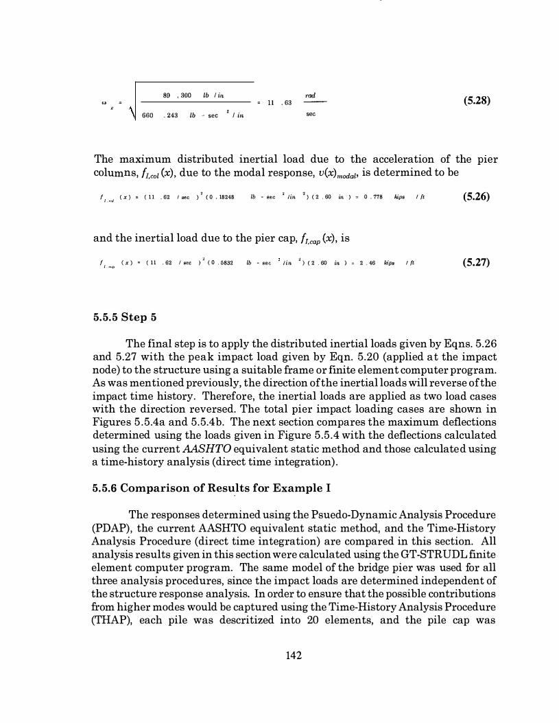
89 , 300 lb l in md (5.28) 11 . 63
660 . 243 lb - sec 2 I in sec
The max1mum distributed inertial load due to the acceleration of the p1er columns, fi,col (x), due to the modal response, v(x) .,wdal> is determined to be
2 2 2 !1 ·"'' ( x ) = ( 11 . 62 I eee ) ( 0 . 18248 lb - sec lin ) ( 2 . 60 in ) "' 0 . 778 kips 1 ft
and the inertial load due to the pier cap, fi.cap (x), is
f ( x ) = ( 11 . 62 / sec ) � ( 0 . 5832 lb - sec lin � ) ( 2 . 60 in ) = 2 . 46 kips 1 ft / , ,,,,
5.5.5 Step 5
(5.26)
(5.27)
The final step is to apply the distributed inertial loads given by Eqns. 5.26 and 5.27 with the peak impact load given by Eqn. 5.20 (applied at the impact node) to the structure using a suitable frame or finite element computer program. As was mentioned previously, the direction ofthe inertial loads will reverse of the impact time history. Therefore, the inertial loads are applied as two load cases with the direction reversed. The total pier impact loading cases are shown in Figures 5 .5.4a and 5.5.4b. The next section compares the maximum deflections determined using the loads given in Figure 5.5.4 with the deflections calculated using the current AASHTO equivalent static method and those calculated using a time-history analysis (direct time integration).
5.5.6 Comparison of Results for Example I
The responses determined using the Psuedo-Dynamic Analysis Procedure (PDAP), the current AASHTO equivalent static method, and the Time-History Analysis Procedure (direct time integration) are compared in this section. All analysis results given in this section were calculated using the GT-STRUDL finite element computer program. The same model of the bridge pier was used for all three analysis procedures, since the impact loads are determined independent of the structure response analysis. In order to ensure that the possible contributions from higher modes would be captured using the Time-History Analysis Procedure (THAP), each pile was descritized into 20 elements, and the pile cap was
142

subdivided into five elements. Member properties and dimensions where given in the previous section in Figures 5.5.1 and 5.5.2. The time- history analysis used the impact loading history for the four 35'x195' barge column developed in Section 3.
All results are for the maximum displacements calculated by each analysis procedure. For the PDAP, the maximum response is the result of the two load cases given by Figures 5.5.4a and 5.5.4b whereas, the maximum response determined using the current AASHTO equivalent static method is the result of the single point load given by Figure 5.5.5. It is important to note that the loading given by Figure 5.3.4a represents the loading which would reasonably be expected to produce the maximum pier displacement and maximum design forces in most of the pier menbers. However, the loading given by Figure 5 .3.4b could conceivably result in the controlling member design forces. Both load cases could be expected to occur over the impact time history and therefore, should be considered in the pier design.
The nodal maximum displacement comparison of the results determined using the PDAP, THAP, and the AASHTO method are given in Table 5.5.1 . Examination of the table reveals that the maximum response determined using the THAP is within 2% of the response determined using the recommended PDAP. However, the AASHTO equivalent static method varies by over 38% from the THAP.
It is important to point out that the design loads determined using the equivalent static method will usually be significantly different from the design loads determined using any of the recommended design procedures. This is due in part to the fact that the AASHTO method neglects the loading that results from the inertial effects. In addition, the peak impact load determined using the equivalent static method does not take into account the dynamic interaction of the individual barges in the flotilla and the dynamic interaction of the barges and the bridge pier.
143

�--··-----·-- 8 /{) ill . �·�----·--�'
C· "'-'"'"' -1 -C_'I_ I iu.
(",If> I = �11_,1),(1f)i) II/
t = -1,5t!U. Or111 f"'i
h ' = -e;;,(i, ,1'·- /5(/.f-' '"'' IJI"I'-' I
I i;r.l in.
•:nil Lm·r"l 1
fN-------�-�-- -�· fl'J
Figure 5.5.1: Psuedo-Dynamic Example Problem.
144

[1n.!IV(n,l "''I ,.,_, : . ,_ ul;--
'-'11(---- ----------------- 8 / i; in. -·----- ----·------ -�
1-e e ��)C i;�-
-- -------
\ 40 in. i'lirHnPleJ
e e I -------] A
;..( �)4 in. )>: - t "!4 in.
Figure 5.5.2: Example Problem Plan View.
145

Node }()
Node ./
Node 1
� -- ·
...,
-L� _L. __ L
Figure 5.5.3: Plane-Frame Model for Example Problem.
146

{A) {B)
Figure 5.5.4: · Psuedo-Dynamic Method Design Load Cases, (A) Maximum Cap Displacement Case, and (B) Possible Impact Member Design Case.
147
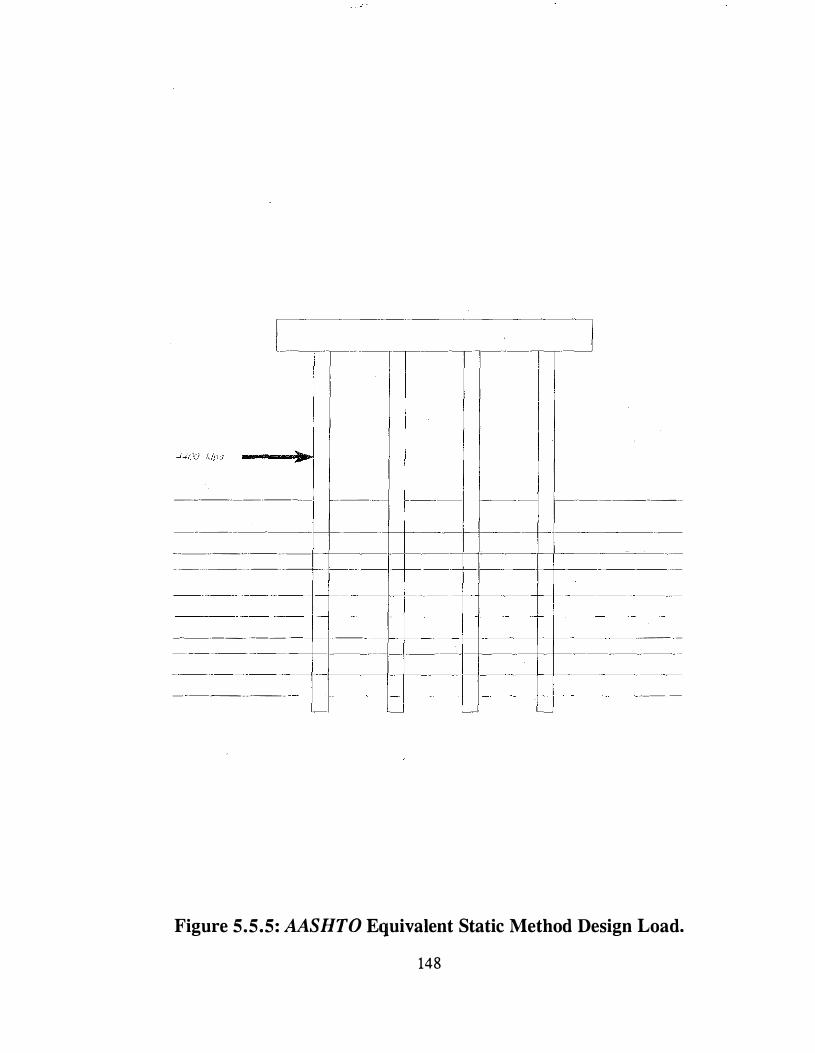
c--�---T- . · -···- �-_]
- - -- --·-- -- --- -
I
-·--- ---------
-·-· ·--- +-- - - · ·+--j-----1--+--·--- --··----· ··-
··-·--- . ---·- f------ ·-1--�
----·--·-L
·----��
· --·-·--- - - - · ·- · · · -- - · ·-1 -----f-- -----f--- - - - - ·-- ·-
= = �=�=--= +=-=:=== -:�== ::::- -= == - ----- --- --- - - -- - - -- --- -- · -·-· -- ·-- --- ···-- ·- --- -·--- 1-[------ · - ------ - -
-. ···-- -- ----·-1---+ -1----- -- - f-- ----1---- -----------· -----··-- --- ----1-- ----+-+---Hi---·---- --- -
- --
Figure 5.5.5: AASHTO Equivalent Static Method Design Load.
148

Table 5.5.1: Predicted Displacements by Analysis Methods.
Displacement (inch)
Location PDAPb
Impact Node 14. 1 1 (node 4•)
Pier Cap 17.61 (node 10")
First Soil Node 2.38 (node 1")
"Note: see Figure 5.5 .1 for node locations. hPDAP: Psuedo-Dynamic Analysis Procedure "THAP: Time-History Analysis Procedure •AASHTO: AASHTO Equivalent Static Method
149
THAP"
13.96
17.45
2.28
AASHTOd
17.8
24.01
4.67
5.6 DESIGN EXAMPLE- II USING THE PDAP
The second design example using the pseudo-dynamic analysis procedure (PDAP) is given here. This example will illustrate impact analysis of the Maysville, Kentucky bridge over the Ohio River for which the statistical analysis design process is given in Appendix I. In addition, this problem will serve to exemplify the analysis of a large non-prismatic bridge pier. The general configuration for the Maysville bridge and piers is shown in Figures 5.6. 1 and 5.6.2
This example follows the step-by-step PDAP procedure presented in section 5.4. In addition, note that all equations use their previously assigned equation numbers. The bridge pier is to be analyzed for impact by a flotilla column of three 55'x300' barges traveling at an impact velocity of v=10.27 fps (see Appendix I, section !.4. 1). This barge type comprises flotilla category HC as given in Section 2, Table 2.3.3 and was determined to be the design flotilla type in the statistical design example given in Appendix I. Each barge has a statisically determined (Section 2) combined dead weight and cargo load of Wb=16,800 kips.
The example pier (shown in Figure 5.6. 1) is comprised of two non-prismatic concrete columns with a variable transverse stiffness of 1=94,800,000 in4 at the column base to 17,300,000 in4 at the column top. The columns are assumed fixed at their base. The pier dimensions are given by Figures 5.6.2 and 5.6.3. The columns are subdivided into ten plane frame beam/column elements (4-DOF/node) between the top pier cap and the footing. Each plane frame element assumes a constant stiffness over the element length equal to the average of the variable stiffness over the element length. The pier cross-frame elements are subdivided into two constant stiffness elements. The plane frame model used is shown in Figure 5.6.4.
5.6.1 Step 1
The first step using the PDAP is to calculate the assumed inertial mode displacement at the impact point location and the concentrated masses or pier cap nodes.
150

90 ft 90 ft ( ) ' ( ) ' 3 2 : 0 . 10
90 ft 90 in
( 460 ft ) ' ( 460 in · ) " 1 . 0 tjr ,.,,(,. II 3 2
460 ft . 460 in .
5.6.2 Step 2
The lead barge kinetic energy,KE1ead• is given by
KE 16 , 800 kips ( 10 . 27 {t / sec ) 2
---'-----'-----'-------''------'-- = 55 , 030 ft - kips 32 . 2 ft . / sec
The lead barge crushing depth is found to be
[( ) ' ]( ) [ 55 , 030 � 10 2 = 1 + - 1 -- 1 + 1 7 LOG 5672 1 57 = 20 . 24 /t
.. ( ( 3 - 1 ) 5 · 576 · · ) ) 17 . 0
(5.28a)
(5.28b)
(5.28c)
(5.28d)
(5.29)
(5.30)
where the KE is in ft-kips, V is in ft/sec, and the crushing depth, aBmult> is given in feet. The peak impact force, P,ax, is found to be
p = [ 110 ( 20 . 24 ) + 1385 ln!l• ] ( 1 . 57 ) · 5670 kips (5.31)
where R8=1.57 for the 55' wide barge.
151

Using the variable member properties given in Figure 5.6.2, the modal mass, M*, modal stiffness, K*, and modal load, P", were integrated numerically using Eqns. 5.5a, 5.5b, and 5.6 with the results given as
•HI
M I , 2 . 41 ( hip - sec 2 1/t ) [ tlr ( x) ] 2 dx
- sec 2 I ft ( 0
.. 23 . 9 kip - sec lft ( 0 . 94 ) � + 23 . 9 kip - sec 2 1ft ( 1 . 0 ) � , 194 . 36 hip - sec � 1 ft (5.32a)
'"' ' K 2 ( 3 ' 500 kip l in ) 94 . 8 X 10
!, jill) '+ 2 ( 3 ' 500 kip l in , 8 X 10 I ,.
49 . 36 ldp l in . 592 . 32 kip I �
P ' ( t ) = ( 5680 kips ) ( 0 . 10 ) " 568 . 0 kips
where
" I o/ C x l I
9
4 L
5.6.3 Step 3
X -- ·
L
J X
9 L n
in ' [ . " ( X ) J 2 dx
, ( x - 90 ) } • " ( x )]
' d(5.32b) in - 40 . 5 xlO in
370
(5.32c)
(5.33a)
(5.33b)
The dynamic magnification factor, DMF, is found by first calculating the inertial mode period, TP, which is
T 2 • ,.
194 . 36 kip - sec I ft
592 . 32 kip I [t 3 . 59 sec
The DMF(TJ is determined (assuming 5% structural damping) by
152
(5.34)
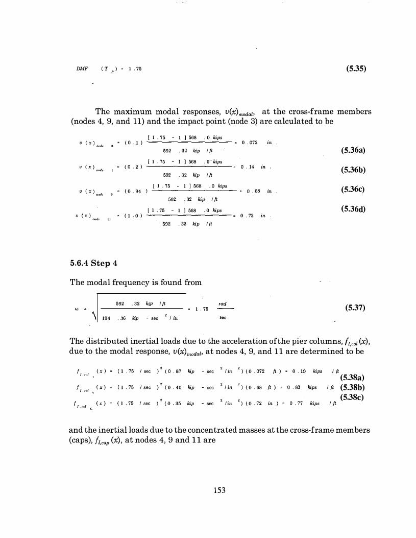
DMF ( T P ) I . 75 (5.35)
The maximum modal responses, v(x),odat• at the cross-frame members (nodes 4, 9, and 11) and the impact point (node 3) are calculated to be
{ I . 75 - I I 568 . 0 kips V ( X ) , ( 0 . I ) , 0 . 072 in norlr• "
(5.36a) 592 . 32 kip I ft
[ I . 75 - I I 568 . o-- kips V ( X ) ( 0 . 2 ) - 0 . 14 in (5.36b) 10nrlo•
592 . 32 kip I ft
[ I . 75 I I 568 . 0 kips (5.36c) V ( X ) ( 0 . 94 0 . 68 in ,,cJ,.
592 . 32 kip I ft
[ I . 75 I I 568 . 0 kips (5.36d) V ( X ) ( 1 . 0 ) 0 . 72 in l!ml<· "
592 . 32 kip I ft
5.6.4 Step 4
The modal frequency is found from
w 592 . 32 kip I {t md
(5.37) 1 . 75
194 . 36 kip - sec 2 I in •eo
The distributed inertial loads due to the acceleration ofthe pier columns, fi '"' (x), due to the modal response, v(x),odal• at nodes 4, 9, and 11 are determined to be
f 1 . ,.,/ ( x ) ( I . 75 I sec ' ) ( 0 . 87 kip - sec ' l in '
) ( 0 . 072 ft ) , 0 . 19 kips I ft (5.38a)
I / . (.,, ( x ) ( I . 75 I sec ' ) ( 0 . 40 kip - sec ' I in '
) ( 0 . 68 tt ) , 0 . 83 kips I ft (5.38b)
f / . , .. / ( X ) ( I . 75 I sec ) ' ( 0 . 35 kip - sec ' I in '
) ( 0 . 72 in ) "' 0 . 77 kips I ft (5.38c)
and the inertial loads due to the concentrated masses at the cross-frame members (caps), !Loop (x), at nodes 4, 9 and 1 1 are
153

I sec ' � ) { 0 ft ) t/ . f<ljJ ( X ) , ( 1 . 75 ) ( 18 . 6 kip - sec I in . 072 , 4 . 11 kips
(5.38a)
tl . <"'J ( X ) , ( 1 . 75 I sec ' ) ( 23 . 9 kip - sec ' l in ' ) ( 0 . 68 ft ) , 50 . 77 kips (5.38b)
' ' in kips (5.38c)
f 1 <"l<jl ( X ) , ( 1 . 75 I sec ) ( 23 . 9 kip - sec I in ) ( 0 . 72 ) , 52 . 70 "
5.6.5 Step 5
The final step is to apply the distributed inertial loads given by Eqns. 5.37 and 5.38 with the peak impact load given by Eqn. 5.31 (applied at the impact node) to the structure using a suitable frame or finite element computer program. As was mentioned previously the direction of the inertial loads will reverse of the impact time history. Therefore, the inertial loads are applied as two load cases with the direction reversed. The next section compares the maximum deflections determined using the PDAP, the current AASHTO equivalent static method, and Time-History Analysis Procedure (THAP).
5.6.6 Comparison of Results for Example II
The responses determined using the Psuedo-Dynamic Analysis Procedure (PDAP), the current AASHTO equivalent static method, and the THAP are compared in this section. All analysis results given in this section were calculated using the GT-STRUDL finite element computer program. The same model of the bridge pier was used for all three analysis procedures, since the impact loads are determined independent of the structure response analysis. Member properties and dimensions where given in the previous section. The time-history analysis used the impact loading history for the three 55'x300' barge column developed in Section 3.
All given results are for the maximum displacements calculated by each analysis procedure. For the PDAP, the maximum response is the result of the peak impact load, the inertial loads due to the cross-frame members, and the distributed column loads. The maximum response determined using the current AASHTO equivalent static method is the result of the single point load.
The nodal maximum displacement comparison of the results determined using the PDAP, THAP, and the AASHTO method are given in Table 5.6.1. Examination of the table reveals that the maximum response determined using the THAP is within 7% of the response determined using the recommended
154

PDAP. However, the AASHTO equivalent static method varies by over 28% from the THAP.
155

- - - �� - - - - - - - - . U r4 - - - - - - - - - - - - - - - - - - - - - - - - - - - - - li�� - - - - - - - - - � � - - -l l I I I I t
Figure 5.6.1:
I I I I I l
1 1\0:;r >'IE'o'
I o>'I[I;' C.J
PLr\N
Fl EVA TION
I E-'·'.T>'/,.,,' I "'''"' •i!
Design Example II Plan and Elevation Views of the Cable Suspended Bridge Over the Ohio River.
156

NOT£: [IF.'4 lVIN<' Nr-'1' To-' �·•. �L£.
� --- /(l,o! II I ' I '
J_ I
,.,,,.,.,, . ,. ...... ,, .. """'""''"
' I 4 -+ 4 L-l__ _l
�-
� - - ! � --·i- --- -''-'·" II _,__ '
I
; £-\.'J PIE!\'
(P/£1\' 5)
N,,,l,• I I
9/.I.U I I
B •l
•'0 • ' II
I = = . ...... -� -111.0 II • I . .
1----
� --�---� � 1- _ •!O.i) II
. . ........ . . ......... : .. E _ , _,_,J .. '.t.. .... .. .... .
{P!Efi' 5)
Figure 5.6.2: Design Example II Bridge Pier.
157

14ft.
<(- -·-·----·---- -20ft.
Section A-A
Section B-B
Figure 5.6.3: Design Example II Pier Cross Sections.
158

J .. J7.JOII,II/JIJ ;,
I � -1,700,IJI!Oin
Impact Point
I � <N,80(},()()(}in
Figure 5.6.4: Design Example II Plane Frame Model.
159

Table 5.6.1: Predicted Displacements by Analysis Methods.
. Displacement (inch)
Location PDAPb
Impact 1 . 1 1 Node
(node 48)
Pier Cap 1 1 .23 (node 38)
Pier Cap 2 6.99 (node 98)
Pier Cap 3 7.76 (node 1 1 8)
•Note: see Figure 5.6.2 for node locations. bPDAP: Psuedo-Dynamic Analysis Procedure "THAP: Time· History Analysis Procedure dAASHTO: AASHTO Equivalent Static Method
160
THAPC AASHTOd
.
1 . 1 5 1 .38
1 .29 1 . 54
7.48 9.13
8.36 10.70
5.7 CONCLUSIONS
The methods presented in this Section is intended to improve the analysis of bridges susceptible to barge flotilla traffic. It was shown that there is a considerable difference between the response calculated using the current AASHTO equivalent static method and the Psuedo-Dynamic Analysis Procedure given in this Section. The current AASHTO analysis procedure does not include the effect of the interaction between the individual barges in the flotilla and the bridge pier. This is significant since the energy lost between the individual barges in the flotilla column was found to be very significant using the analysis techniques given in this Section.
Another important difference between the two methods is that the current AASHTO analysis procedure neglects the member loading that results due to the inertial effects of the impact loading time history, whereas the inertial loading is included with the Psuedo-Dynamic Procedure. In addition, the effect of inertial load reversal over the structure response time-history for member design can be considered by using the load cases presented in the design example.
161

6.0 CONCLUSIONS AND FURTHER RESEARCH NEEDS
6.1 GENERAL SUMMARY
Presented in this study is a data collection and analysis procedure whereby Methods I and II of the AASHTO Specification for Vessel Collision may be applied to the design of inland waterway highway bridges. No known bridge has been designed using either method due to the variability of the barge sizes and flotilla types. A design example is included in Appendix I where an actual bridge was designed using the statistical procedures outlined in this study.
Additionally, alternate dynamic analysis procedures, which more accurately model the barge-bridge response forces, are presented. The design procedures are presented in Section 5 and Appendix III in a format that could be included in the AASHTO Guide Specification for Collision Design of Highway Bridges. The current AASHTO equivalent static method neglects the important dynamic interaction that occurs between the individual barges of the flotilla column and the bridge pier. In addition, the current AASHTO analysis method neglects the distributed member loads that results due to the inertial effects of the impact loading.
A design example was also included in Section 5 to illustrate the use of the. psuedo-dynamic analysis procedure. The results indicate there is up to a 38% difference between the deflections predicted by the suggested analysis procedure and the AASHTO procedure. In addition, a design example is presented in Appendix 6 which shows that there was also significant difference between the impact spectrum analysis method and the current AASHTO equivalent static method.
6.2 DESIGN FLOTILLAS
A method has been provided by which available barge and flotilla data may be utilized to develop the risk assessment procedures for vessel impact design problems in accordance with the 1991 AASHTO Guide Specification. For illustrative purposes, this study concentrated on barge traffic on Kentucky's
162

navigable waterways. However, the methodologies presented in this study are applicable to all navigable inland waterways in the United States and the World. Results generated in this study reflect a statistical analysis conducted on the data obtained from the U.S. Coast Guard, the U.S. Army Corps of Engineers, and the American Waterways Operators. The data gathered in order to apply design Methods of the guide specification are: 1) barge size and capacities, 2) the number of barges in a flotilla column and row, 3) river elevations, 4) flotilla transit velocity, and 5) probabilities of aberrancy.
The barge types defined in this study are based on the U.S. Army Corps of Engineers' barge length and width designation system. Flotillas are generally made up of mostly the same barge size and type. Nevertheless, it was found that a very large variation in the flotillas using the Kentucky waterway system still exists. Therefore, a probability based approach was adopted to calculate the number of barges comprising a flotilla. Flotillas are then categorized based upon the primary barge type in the train.
.
Maximum attainable speeds for fully loaded flotillas under ideal conditions, as determined by a survey of the American Waterways Operators and the U.S. Coast Guard Captain of the Port, Louisville, KY, are reported. Values used for flotilla transit velocity are: I) 7 mph for the Ohio and Tennessee Rivers, and 2) 5 mph for the Cumberland and Green Rivers. Since the Performance Monitoring System Database does not currently document any flotilla traffic on_the Kentucky River, the minimum value of 5 mph should be used for flotillas navigating this nver.
The probabilities of aberrancy (P A) have been reported for different ranges along the navigable waterways of Kentucky in other sources. For most ranges, the values are near what would be calculated using the AASHTO Guide Specification (1991) approximate method. Sometimes the probabilities are quite high. However, careful examination of the historical casualty data supports the accuracy of the results. It is recommended that the probability of aberrancy for
· a section of river under consideration be used in design calculations, instead of a weighted average PA for the entire river.
Based on section 4.8.2 of the AASHTO Guide Specification (1991), the acceptable annual frequency of collapse, AFc, was reported as 0.0001 for critical bridges and, AF, 0.001 for regular bridges. The acceptable annual frequency of bridge collapse should be distributed, either equally or at the designers discretion, over all piers located within the waterway. A recommendation to distribute the annual frequency of collapse to each pier based on its percentage value of the replacement cost of the structure was reported. The summation of the annual
163

frequencies of collapse for all barge size categories, with respect to the individual piers, should then be less than or equal to the AFP assigned to each component.
It is recommended that the impact loads for the loaded barge flotillas be applied in conjunction with 100% of long-term scour plus the local scour caused by a Q5 flood event. The impact loads fur a single free-floating loaded barge (as per the Kentucky Transportation Cabinet design minimum assumption) should be applied with the scour caused by the Q100 flood event plus 100% of the longterm river bed aggradation or degradation. Currently the AASHTO Guide Specification gives no guidance for using future barge traffic projections when considering the design life of the bridge. Therefore, it is recommended that a 50-year design life be used.
The equivalent static impact loads and their associated frequencies are derived for a bridge over the Ohio River (in Appendix I). The impact loads calculated using the AASHTO formulas probably give unrealistic results since they are based on relationships which neglect energy dissipation due to crushing and friction and dynamic load magnification effects.
The lateral capacities ofthe bridge piers required using design Method II of the AASHTO Guide Specification (1991) are found to be more conservative than the lateral capacities required using the less rigorous design Method I procedure. However, the results ofthis study indicate that, after the initial effort by a state or agency of accumulating and processing the necessary information, further designs using Method II can be completed with economy equal to designs completed using Method I.
6.3 ANALYSIS METHODS
Revisions to the current Guide Specification are presented for three levels of analysis which are
1): Psuedo-Dynamic Analysis Procedure (PDAP) 2): Impact Spectrum Analysis Procedure (ISAP) 3): Time-History Analysis Procedure (TRAP)
The level of analysis is dictated by the importance classification of the bridge, the dynamic load (or acceleration), whether the bridge is critical or non· critical, and whether the bridge is regular or irregular.
164
In order to develop the loading functions, the flotilla was assumed to impinge perpendicularly on a rigid support (pier). If it is further assumed that the support crushes only the section of the barge adjacent to the support, then the barge may be divided into two regions: A) a non-linear crushing zone and B) an elastic zone.
A non-linear dynamic finite element computer program was developed in order to generate the barge flotilla impact loading functions. The non-linearity in the model is a result of the crushing ofthe barges at the contact point between other barges or the bridge pier. The total impact force on the support node includes the force resulting from the change of momentum of the crushed mass. The barge stiffness is taken from the bilinear load deformation relationship (Section 3 . 12, AASHTO Guide Specification). The flotilla impact loading functions are used to develop the impact loading spectrums. An impact loading spectrum is analogous to an earthquake displacement response spectrum with the exception that the loading is the result of mass excitation rather than base excitation.
In order to determine the dynamic bridge response, the total dynamic response is resolved into the contribution of the low and high modes. It was shown that the response of higher frequency modes can be calculated by static analysis because their inertial effects are negligible. Therefore, the response can be approximated by the contribution of the inertial response plus the static response.
For the simplified analysis procedure, only a single dynamic mode was considered to contribute significantly to the total dynamic response; therefore, the free vibration modal analysis is not required. Rather, only a static analysis is needed where the structure is loaded with the maximum magnitude ofthe barge impact force time history at the impact point plus the distributed inertial loading determined from the impact spectrum and the assumed mode shape.
The modal impact method is similar to the preceding simplified impact method. However, the dynamic response of the bridge is approximated by a combination of modes (multi -modal analysis). Therefore, a free-vibration analysis must be conducted in order to determine the mode shape vectors. An important difference between impact analysis and seismic analysis is the possibility that higher mode shapes can contribute significantly to the total response of the bridge during impact. However, the procedure given allows for the determination of only the lower mode shapes with the inclusion of the higher mode shape effects accomplished in a manner similar to the aforementioned simplified impact
165

method. Therefore, the modal analysis can be conducted using current design software.
Generally, an impact time-history analysis of a bridge would be required for major bridges. However, a time-history analysis allows for an examination of the effect of several important factors during a barge-bridge collision that can not be included in a modal analysis which include
• Non-Linear Dynamic Soil-Structure Interaction, • Plastic Hinge formation • Large Deformation Effects
A drawback of this type of analysis is that it requires a knowledge of the dynamic and cyclic properties of the soil at the bridge site. However, a more accurate determination of the true dynamic response of the structure is afforded by this method which may significantly change the structure design.
6.4 FUTURE RESEARCH NEEDS
Future research needs can be classified in two broad catagories; loading time histories, and bridge dynamic response. These catgories will be covered in the following sections.
6.4.1 Loading Time Histories
Due to the complexity of modeling the barge during impact, which not only includes the crushing of each ofthe barges in the flotilla but also the crushing of the barge cargo, impact testing of individual and groups of barges should be conducted to verify the impact load time histories derived in this study. The impact testing could includ the effects of various cargo on the load time histories. In addition, the effect of angle of impact on the loading time histories needs to be investigated.
6.4.2 Bridge Dynamic Response
The procedures given in this study provide a method by which the dynamic response of a bridge to barge impact can be examined. But a detailed study is needed where the sensitivity ofthe bridge to several important structural effects is investigated. These should include the effects of large deformations, and
166

plastic hinges on the overall structural response. Plastic design could be investigated with the results of this study. Design ductility demand/capacity ratios for impacted columns, etc. could be determined in order to prevent collapse but allow for inelastic load redistribution.
167
BIBLIOGRAPHY
AASHTO (1991). "Guide Specification and Commentary for Vessel Collision Design of Highway Bridges. Volume I: Final Report". American Association of State and Highway Transportation Officials, Washington, D.C.
Bathe, K.J. and Cimento, A.P. (1980). "Some Practical Procedures for the Solution of Nonlinear Finite Element Equations." Computer Methods in Applied Mechanics and Engineering, Vol. 22, pp. 59-85.
Bathe, K.J.; Wilson, E.L. (1972). Numerical Methods in Finite Element Analysis, Prentice-Hall. Englewood Cliffs. New Jersey.
Bein, P. (1993). "Risk Modeling of Vessel Impacts on a Multispan Bridge." Structures under Shock and Impact II. Matt MacDonald Group, U.K., pp. 265-275.
Blandford, G.E. and Glass, G.C. (1987). "Static/Dynamic Analysis of Locally Buckled Frames."Journal of Structural Engineering, ASCE, Vol l13, No. 2, pp. 363-380.
Blok, J.J.; Delker, J.N. (1979). On hydrodynamic aspects of ship collision with rigid or non-rigid structures. OTC study 3664. presented at the Eleventh Annual Offshore Technology Conference. Houston, Texas.
Brink-Kjoer 0. et al. ( 1983). Modelling of ship collision against protected structures. In Proceeding. IABSE Colloquium Copenhagen Vol. 42. pp. 14 7-64.
Bruen, F.J.; and Vivitrat, V. (1984). Ice force prediction based on strain-rate field. In Third International Offshore Mechanics and Arctic Engineering Symposium OMAE 84 Vol. 3, pp. 27-81.
Chang, P.T. et al. (1980). A rational methodology for the prediction of structural response due to collisions of ships. SNAME Annual Meeting, New York, 13-15, study no. 6.
Crisfield, M.A. (1988). "Numerical Methods for the Non-linear Analysis of Bridges." Computers and Structures, Vol. 30, No. 3, pp. 637-644.
168
"Criteria for: The Design of Bridge Piers with Respect to Vessel Collision in Louisiana Waters." (1984). Report Prepared for Louisiana Department of Transportation and Development and the Federal Highway Administration, Modjeski and Masters Consulting Engineers, New Orleans, LA.
Davies, G.A.(1984). Structural Impact and Crashworthiness Vol. 1 chapter 7. Elsevier.
Emori, R. l . (1968), Analytical approach to automobile collisions. Automotive Engineering Congress. Detroit, Michigan, study no 680016.
Emori, R.I. (1968). Analytical approach to automobile collisions. SAE Study 180016. Society of Automobile Engineers, USA.
Facmillan, R.H. Dynamics of Vehicle Collisions. Special Publications SP5. Inderscience Enterprises, Jersey, UK.
Furness, 0. and Amdahl Journal (1979). Computer simulation study of offshore collisions and analysis of ship platform impacts. Study presented at The Second International Symposium on Offshore Structures, Brazil, October 1979 (also in Applied Ocean Research 2, no 3, 119-27, 1980).
Furness, 0. and Amdahl Journal (1980). Ship collisions with offshore platforms. DNV study 80-P080, presented at Intermaritec '80 Conference, Hamburg, September 1980.
Grime, G. and Jones, I.S. (1969). Car collisions , the movement of cars and their occupants. Proceedings 1 . Mechanical Engineering 184 no 5.
Guttman, S. I . ; Pushar, F. ; Journal and Bea, R.G. (1984). Analysis of offshore structures subject to arctic ice impacts. In Proceedings of the Third Symposium on Offshore Mechanics and Arctic ln Engineering pp. 238-45. New Orleans, Louisiana.
Guide specification and commentary for vessel collision design of highway bridges, Volume I: Final Report. (1991). American Association of State Highway and Transportation Officials (AASHTO), Washington, D.C.
169
Hagiwara, K. et al. (1983). A proposed method of predicting ship collision damage. International Journal of lmpact Engineering 1 257-80.
Kennedy, R.P. (1966). Effects of an Aircraft Crash into a Concrete Building. Holmes and Narver Inc., Anaheim, Ca.
Knapp, A. E.; Green, D. J. ; Etie, R.S. (1984). Collision of a tanker with a platform OTC study 4 734, presented at the Sixteenth Annual Offshore Technology Conference, Houston, Texas.
Koehler, P.E. and Jorgensen, L. (1985). Ship impact ice analysis. In Proceedings of the Fourth Symposium on Offshore Mechanics and Arctic Engineering ASME-Omae pp. 344-50. Dallas, Texas, February 1985.
Larsen, C.; Engseth, A. G. (1979). Ship collision and fendering of offshore concrete structures. Study EUR 17, presented at The First European Petroleum Conference, London.
Lexington Herald-Leader. (1993). (July 18), Al.
Lexington Herald-Leader. (1995). (April 24), B3.
Low, H.Y.; Worley, C.T. (1983). Indentation tests of simplified models of ships' structures. In Proceedings ofthe IABSE Colloquium on Ship Collision with Bridges and Offshore Structures pp. 213-20. Preliminary report. Copenhagen.
Macaulay, M.A. and Macmillan, R.H. (1968). Impact testing of vehicle structures. In Proceedings of the 12th FISITA Congress. Barcelona.
Minorsky, V.V. (1959). An analysis of ship collisions with reference to nuclear power plants. Journal of Ship Research 3 1-4.
Nagasawa, H.; Arita, K.; Tani, M. and Oka, S. (1977). A study on the collapse of ship structure in collision with bridge piers. Journal Soc. Nav. Arch. Japart 142.
Neilson, I.D. et al. (1968). Controlled impact investigations. TRRL Report LR 132. Transport Road Research Laboratory, Crowthorne, UK.
Riera, J. (1980). A critical reappraisal of nuclear power plant safety against accidental aircraft impact. Nuclear Engineering Design, 57.
170
Rinehart, J.S. (1950). Some observations on high-speed impact. Naval Ordinance Test Station RRB-50. Felix Helie, Paris, France.
Roland, B. ; Olsen, T.; and Skaare, T. (1982). Ship impact on concrete shafts. Study EUR 305, presented at the Third European Petroleum Conference, London.
Samuelides, E. and Frieze, P.A. (1983). Strip model simulation for low energy impacts on flat-plated structures. International Journal of Mechanical Sciences. 25 669-86.
Soreide, T.H. (1981). Ultimate Load Analysis of Marine Structures. Tapir, Trondheim. 2 .118 JABSF (1983) Ship collision with an offshore structure. IABSE Colloquium,Copenhagen.
Stephen, A. & Silter, G. (1977). Full-scale tornado-missile impact tests. Fourth International Conference on Structural Mechanics in Reactor Technology (SMiRT),Berlin, 1977, study Jl0/1.
Wagner, R. (1978). Compatibility in frontal collisions. In Proceedings of the 17th FISITA Congress Budapest.
Wall, J.G. et. al. (1970). Comparative head-on impact tests. TRRL Report LR 155.Transport Road Research Laboratory, Crowthorne, UK.
Watson, A. & Ang, T. (1984). Impact response and post-impact residual strength of reinforced concrete structures. International Conference and Exposition of Structural Impact and Crashworthiness, Imperial College, London, UK.
Whitney, M.W.; Harik, I.E.; Griffin, J.J.; and Allen, D.L. (1996). "Barge Collision Design of Highway Bridges." ASCE Journal of Bridge Engineering, Vol.l, No. 2, pp. 47-58.
Whitney, M.W.; Harik, I.E.; Griffin, J.J. ; and Allen, D.L. (1994). "Barge Traffic on Kentucky Rivers." Res. Rep. KTC-94-15, University of Kentucky, Lexington, KY.
Winter, R.; Pifko, A.B. (1988). Finite element crash analysis of automobiles and helicopters. In Structural Impact and Crash Worthiness (Ed. by Journal Morton), Vol. II, pp. 278-309. Conference studys. Elsevier.
171

Woisin, G. (1977). Conclusion from collision examinations for nuclear merchant ships in the FRG. In Proceedings of the Symposium on Naval Submarines. Hamburg.
Yagawa, G. ; Ohtsubo, H.; Takeda, H.; Toi, Y.; Aizawa, T.; and Ikushima T. (1984). A round robin on numerical analyses for impact problems. Nuclear Engineering Design, 78, 377-87.
Young, C.W. (1975). Simplified analytical impact model with lateral loading. SAND-4-1635. Sandia National Laboratory, Albuquerque, NM.
Zayas, V.A.; Dao B.V.; and Hammett, D.S. (1985). Experimental and analytical comparisons of semi-sumbersible offshore rig damage resulting from a ship collision, Offshore Technologv Conference. Houston, Texas.
Zhong, Z.H. (1989). Evaluation of friction in general contact-impact interfaces. Communications in Applied Numerical Methods.
Zienkiewicz, O.C. (1977). Finite Element Analysis in Engineering Science. McGraw Hill. London.
172
ADDITIONAL REFERENCES
ADINA Engineering (1984). Automatic Incremental Nonlinear Analysis. Users Manual. ADINA Engineering Inc, MIT, Massachusetts, USA.
AM (1982). Concrete Structures under Impact and Impulsive Loading. Bundesanstalt fur Materialprufung, Berlin.
Andrews, K.P.F. et al. (1983). Classification of the axial collapse of cylindrical tubes under quasi-static loading. International Journal of Mechanical Sciences vol. 2, 678-96.
ASCE Task Committee on Finite Element Analysis of RC Structures (1982). "Finite Element Analysis of Reinforced Concrete". American Society of Civil Engineering Committee on Concrete and Masonry, A.H. Nilson, Chairman, Cornell University, Ithaca, NY.
Atluri, S.N. (1984). On constitutive relations at finite strain: hypoelasticity and elasto- plasticity with isotropic or kinematic hardening. Computational Methods in Applied Mechanics in Engineering, 43 137-71 .
Backman, M.E. and Goldsmith, W. (1978). The mechanics of penetration of projectiles into targets. Int. Journal Engineering Sci. 1691-99.
Barr, P. et al. (1982) An experimental investigation of scaling of reinforced concrete structures under impact loading. In Design for Dynamic Loading. Construction Press, London, UK.
Barr, P. et al. (1983). Experimental studies of the impact resistance of steel faced concrete composition. Seventh International Conference on Structural Mechanics in Reactor Technology (SMiRT), 1983, study J8/4, Chicago, USA.
Bate, S. (1961). The effect of impact loading on prestressed and ordinary reinforced concrete beams. National Building Studies Research Study 35.
Bathe, K.J. and Bolourchi, S. (1979). "Large Displacment Analysis of ThreeDimensional Beam Structures." International Journal for Numerical Methods in Engineering, Vol. 14, No. 7, pp. 961-986.
173

Bathe, K.J. and Cimento, A.P. (1980). "Some Practical Procedures for the Solution of Nonlinear Finite Element Equations. " Computer Methods in Applied Mechanics and Engineering, Vol. 22, pp. 59-85.
Bathe, K.J. (1971). Solution methods for large generalized Eigenvalue problems in structural engineering. SESM Rep. 71-120. Civil Engineering Department, University of California, Berkeley.
Bathe, K.J.; Wilson E.L. (1972). Numerical Methods in Finite Element Analysis, Prentice-Hall. Englewood Cliffs. New Jersey.
Beriaud, C. et al. (1977). Local behaviour of reinforced concrete walls under hard missile impact. Fourth International Conference on Structural Mechanics in ReactorTechnology (SMiRT), Berlin, 1977, study J7/9.
Bernard, R.S.; Hanagud, S.V. (1975). Development of a projectile penetration theory, Report 1 , Penetration theory for shallow to moderate depths. Technical Report S-75-9. Soils and Pavements Laboratory, US Army Corps of Engineers Waterways Experiment Station, Vicksburg, Miss.
Bernard, R.S. (1976). Development of a projectile penetration theory. Report 2, Deep penetration theory of homogeneous and layered targets. Technical Report S-75-9. Soils and Pavements Laboratory. US Army Corps of Engineers Waterways Experiment Station, Vicksburg, Miss.
Bernard, R.S. and Hanagud, S.V. (1975). Development of a projectile penetration theory. Technical Report S-75-9. US Army Corps of Engineers Waterways Experiment Station.
Bernard, R.S. (1976). Development of a projectile penetration theory report 2 : deep penetration theory for homogeneous and layered targets. Technical Report S-75-9 US Army Corps of Engineers Waterways Experiment Station, Virginia, USA.
Birkhoff, G.; MacDougall, D. ; Pugh, E. ; & Taylor, G. (1948). Explosives with lined cavities. Journal Applied Physics 1991.
Billing, I. (1960). Structure Concrete. Macmillan, London.
Biggs, J. M. (1964). Introdtroduction to Structural Dynamics chapter 2. McGraw-Hill.
174

Blandford, G.E. (1988). "Static Analysis of Flexibly Connected Thin-Walled Plane Frames. "Computers and Structures", Vol. 28, No. 1 , pp. 105-113.
Blandford, G.E. (1990). "Thin-Walled Space Frames With Geometric and Flexible Connection Nonlinearities. "Computers and Structures, Vol. 35, No. 5, pp. 609-617.
Brown, D. and Bollman, H. (1991). "Pile Supported Bridge Foundations Designed for Impact Loading." Transportation Research Record, No. 1331, pp. 87-91.
Blok, J.J.; Delker, J.N. (1979). On hydrodynamic aspects of ship collision with rigid or non-rigid structures. OTC study 3664. presented at the Eleventh Annual Offshore Technology Conference. Houston, Texas.
Bodner, S.R.; Symonds, P.S. (1972). Experimental and theoretical investigation of the plastic deformation of cantilever beams subjected to impulsive loading. Journal of Applied Mechanics December, 719-28.
Brink-Kjoer, 0. et al. ( 1983). Modelling of ship collision against protected structures. In Proceeding. IABSE Colloquium Copenhagen Vol. 42. pp. 14 7-64.
Bruen, F.J. and Vivitrat, V. (1984). Ice force prediction based on strain-rate field. In Third International Offshore Mechanics and Arctic Engineering Symposium OMAE 84 Vol. 3, pp. 27-81.
Burgess, W. & Campbell-Allen, D. (197 4). Impact resistance of reinforced concrete as a problem of containment. Research Reporf no R251. School of Civil Engineering, University of Sydney.
Butler, D.K. (1975). An analytical study of projectile penetration into rock. Technical Report S-7 5-7. Soils and Pavements Lahoratory, US Army Corps of Engineers Waterways Experiment Station, Vicksburg, Miss.
Butler, D.K. (1975). Pretest penetration for DNA rock penetration experiments at a sandstone site near San Ysidro, New Mexico. Soils and Pavements Laboratory, US Army Corps of Engineers Waterways Experiment Station, Vicksburg, Miss.
Byers, R. K. and Chabai, A. Journal (1977). Penetration calculations and measurements for a layered soil target. Interltational Journal for
175
Numerical and Analytical Methods in Geomechanics Vol. 1 107-38.
Cammaert, A.B. and Tsinker, G.B. (1981). Impact of large ice floes and icebergs on marine structures. In Proceedings of the Sixth International Conference on Port and Ocean Engineering under Arctic condition.s Vol. II, pp. 653-67. Quebec City, Canada.
Carr, H. H. Analysis of head failure in aircraft torpedoes. NOTS Navorcl Report 1019 Patent Office Library, London.
Chen, W.F. and Atsuta, T. (1977). Theory of Beam-Columns. Vol. 2, McGrawHill, Inc., New York, NY.
Chen, H. (1990). Nonlinear Space Analysis Including Flexible Connection and Bifurcation Behavior. Ph.D. Dissertation, University of Kentucky, Lexington, KY.
Chen, H. and Blandford, G.E.(1991a). "Thin-Walled Space Frames. I: Large Deformation Analysis Theory." Journal of Structural Engineering, ASCE, Vol. 117, pp. 2499-2520.
Chen, H. and Blandford, G.E. (1991b). "Thin-Walled Space Frames. II: Algorithmic Details and Applications." Journal of Structural. Engineering, ASCE, Vol. 117, pp. 2521-2539.
Crisfield, M.A. (1988). "Numerical Methods for the Non-linear Analysis of Bridges." Computers and Structures, Vol. 30, No. 3, pp. 637-644.
Chen, E.P. and Sih, G.C. (1977). Transient response of cracks to impact loads. In Elasto-Dynamic Crack Problems, Vol. 4. Noordhoff, Groningen. Leyden.
Clint, M. ; Jennings A. (1970). The evaluation of Eigenvalues and Eigenvectors of real symmetric matrices by simultaneous iteration. Comput. Journal, 13(1).
Continental shelf. Collection and preparation of data. Part report no. 7. Reported ship impacts with fixed and mobile offshore platforms. Dll V Report FDI v /20-82-021.
Conway, M.D. ; Jakubowski M. (1969). Axial impact of short cylindrical bars. Journal of Applied Mechanics 36-80.
176

Coppa, A. (1960). On the mechanics of buckling of a cylindrical shell under longitudinal impact. Tenth International Congress Applied Mech. , September 1960, Stressa, Italy.
Craig, R.R. (1981). Structural Dynamics. An Introduction to Computer Methods. Wiley.
Creighton, D.C.(l982). Non-normal projectile penetration in soil and rock: user's guide for computer code ENC02D . Technical Report SL-8-7. US Army Engineering Waterways Experiment Station, Vicksburg, Miss.
Davison, L. and Graham, R.A. (1979). Shock compression of solids. Phys Rep. 55 255-379. 2.193 Meyer M.A. and Aimone C.T. (1983) Dynamic fracture (spalling) of metals. Prog.Mat. Sci. 28, 1-96.
Davies, G.A.(1984). Structural Impact and Crashworthiness Vol. 1 chapter7 .Elsevier.
Davie, T.N. & Richgels, A.M. (1983). An earth penetrator code. Sandia Report (.SAND-255). Sandia National Laboratories, Livermore, California.
de Oliveira, J.G. (1981). Design of steel offshore structures against impact loads due to dropped objects. Report No 8 1-6. Department of Ocean_ Engineering, Massachusetts Institute of Technology, Cambridge, Ma.
Derbalian, G.; Fowler, G.; and Thomas Journal (1984). Three-dimensional finite element analysis of a scale model nuclear containment vessel. American Society of Mechanical Engineering, study 84-PVP-S.
Donea, J. (1983). Arbitrary Lagrangian-Eulerian finite element methods. In Computational Methods for Transient Analysis, (Ed. by T. Belytschko and T.JournalR. Hughes), pp. 473-516. Elsevier.
Drucker, D.C. (1951). A more fundamental approach to plastic stress-strain relations. Proceedings. 1st US National Congress on Applied Mechanics, pp. 487-91. Pasadena, USA.
Duncan, J.M. ; Byrne, P.M.; Wong, K.S . ; and Mabry, P. (1980). Strength stress-strain and bulk modulus parameters for finite element analyses of stresses and movements in soil masses. Report No UCBI GT178-02. Department of Civil Engineering, University of California. Berkeley.
177

Duncan, J.M.; Chang, C.Y. (1970). Non-linear analysis of stress and strain in soils. Journal Soil Mechanics Foundation Division, ASCE, 96(SM5), 1629-51.
Emori, R. l . (1968). Analytical approach to automobile collisions. Automotive Engineering Congress. Detroit, Michigan, study no 680016.
Emori, R.I. and Tanin, F. (1970). Vehicle trajectories after intersection collision impact.SAE Study 700176. Society of Automobile Engineers.
Fredriksson, B.; Mackerle, J. (1983). Structural Mechanics Finite Element Computer Programs, 4th edn. Advanced Engineering Corporation, Linkoping, Sweden.
Friedrichs, K.O. (1941). On the minimum buckling load for spherical shells. In Theodore von Karman AnersaryVolurne pp. 258-72. CIT, Pasadena, USA.
Glass, J. & Bruchey, W. (1982). Internal deformation and energy absorption during penetration of semi-infinite targets. In Proceedings of the Eighth International Symposium on Ballistics NASA, Langely, USA.
Glasstone, S. & Dolan, P.Journal (1977). The Effects of Nuclear Weapons. U.S. Department of Defense, Washington.
Goldsmith, W. (1960). Impact The Theory and Physical Behaviour of Colliding Solids. Edward Arnold, London.
Guttman, S.l.; Pushar, F.Journal and Bea, R.G. (1984). Analysis of offshore structures subject to arctic ice impacts. In Proceedings of the Third Symposium on Offshore Mechanics and Arctic ln Engineering pp. 238-45. New Orleans, Louisiana.
Hallquist, J.O. (1986). NIKE2D: A vectorized, implicit, finite deformation, finite element code for analyzing the static and dynanlic response of 2-D solids. UCID-1677 Re. 1. University of California.
Hallquist, J.O. & Benson, D.Journal (1986). DYNA3D user's manual (nonlinear dynamic analysis of structures in three dimensions). Report UCID-19592. Rel ision 2. University of California, Lawrence Livermore National Laboratory.
178

Hallquist, J.O. (1984). NIKE3D: an Implicit, Finite Deformation. Finite Element Code for Analyzing the Static and Dynamic Response ofThree-Dimensional Solids. Uc/D-lly7 re.5. University of California.
Hammel, J. (1979). Impact loading on a spherical shell. Fifth International Conference on Structural Mechanics in Reactor Technology (SMiRT), Berlin.
Hargrave, M.W.; Hansen A. G. , Hinch, J.A. (1989). A summary of recent side impact research conducted by the Federal Highway Administration. SAE Technical Study No 890377. Society of Automotive Engineers, Warrendale, Pa.
Henrych Journal (1979). The Dynamics of Explosion and its Use. Elsevier, Amsterdam.
Hetherington, W.G. (1979). Floating jetties- construction, damage and repair. Study no. 3 from the Concrete Ships and Floating Structures Convention.
Housen, K.; Schmidt, R.; & Holsapple, K. (1983). Crater ejecta scaling laws: fundamental forms based on dimensional analysis. Journal Geophysic Res. 88.
-
Hughes, T.J.R.; Pister, K.S. ; Taylor R.L. (1987). Implicit-explicit finite elements in nonlinear transient analysis. Computer Methods in Applied Mechanics in Engineering 17/18, 15-22.
Hughes, T.J.R.; Levit, L.; Winget, J.M.; (1983). An element-by-element solution algorithm for problems of structural and solid mechanics. Methods in Applied Mechanics in Engineering, 36 - 54.
Hughes, G. & Speirs, D. (1982). An investigation of the beam impact problem. Technical Report 546C, British Cement Association.
Hurty, W.C.; Rutinstein, M.F. (1964). Dynamics of Structures. Prentice-Hall.
Isaacson, E .; Keller, H.B. (1966). Analysis of Numerical Methods. Wiley, New York.
Ito, Y.M.; Nelson, R.B.; & Ross-Perry, F.W. (1979). Three-dimensional numerical analysis of earth penetration dynamics. Report DNA 544F. Defense Nuclear Agency, Washington DC, USA.
179

Ivey, D.L.; Ruth, E. ; and Hirsch, T.Journal (1970). Feasibility of lightweight cellular concrete for vehicle crash cushions. Study presented at the Annual Meeting of the Highway Research Board, Washington DC.
Jankov, Z.; Turnham, ''J.; & White, M. (1976). Missile tests of quarter-scale reinforced concrete barriers. In Proceedings of the Symposium on Tornadoes Assessmnent of Knowledge and Implicationts for Man. Texas University, June 1976.
Johnson, G.R. & Stryk, R.A. (1986). Dynamic-Lagrangian computations for solids, with variable nodal connectivity for severe distortions. Int. Journal Num. Methods Eng 23, 5022.
Johnston, P.R. and Weaver, W. Jr (1987). Structural Dynamics by Finite Elements. Prentice-Hall, Englewood Cliffs, Njournal.
Jonas, W. and Rudiger, E. (1977). Experimental and analytical research on the behaviour of reinforced concrete slabs subjected to impact loads. Fourth International Conference on Structural Mechanics in Reactor Technology (SMiRT), Berlin, study J7/6.
Jones, N. & Wierzbicki, T. (1983). Structural Crash Worthiness. Butterworths, London.
Johnson, W. (1972). Impact Strength of Materials. Edward Arnold, New York.
Jones, L.S. (1975). Mechanics of roll-over as the result of curb impact. SAE Study 750461. Society of Automobile Engineers.
Kanto, Y. and Y agawa, G. (1990) Finite element analysis of dynamic buckling with contact. Japan Society of Mechanical Engineering, Series, 51, 2747-56.
Kar, A.K. (1979). Impactive effects of tornado missiles and aircraft. Transactions. ASCE 105, ST2, 2243-60. (Also Loading time history for tornado generated missiles. Nuclear Engineering Design 51, 487-93, 1979.
Kar, A. K. (1977). "Projectile Penetration into Buried Structures". Journal Structural Division ASCE study 13479STI.
Kennedy, R.P. (1966). Effects of an Aircraft Crash into a Concrete Building. Holmes and Narver Inc., Anaheim, Ca.
180

Kinslow, R. (Ed.) (1970). High Velocity Impact Phenomena. Academic Press. Nowacki W.K. (1978) Stress Waves in Non-Elastic Solids. Pergamon.
Knapp, A.E. ; Green D.J.; Etie, R.S. (1984). Collision of a tanker with a platform OTC study 4734, presented at the Sixteenth Annual Offshore Technology Conference, Houston, Texas.
Koehler, P .E. and Jorgensen, L. (1985). Ship impact ice analysis. In Proceedings of the Fourth Symposium on Offshore Mechanics and Arctic Engineering ASME-Omae pp. 344-50. Dallas, Texas, February 1985.
Kufuor, K. & Perry, S. (1984). Hard impact of shallow reinforced concrete domes. International Conference · and Exposition of Structural Impact and Crashworthiness,Imperial College. London, UK.
Kulak, R.F.; Fiala, C. (1983). NEPTUNE: a system offinite element programs for three-dimensional non-linear analysis. Nuclear Engineering Design, 106, 47-68.
Kulak, R.F. (1989). Adaptive contact elements for three-dimensional explicit transient analysis. Computer Methods in Applied Mechanics and Engineering, 72, 125-51.
Larsen, C. ; Engseth, A. G. (1979). Ship collision and fendering of offshore concrete structures. Study EUR 17, presented at The First European Petroleum Conference, London.
Lee, E.H. and Morrison, Journal A. (1956). A comparison of the propagation of longitudinal waves in rods of viscoelastic materials. Journal of Polymer Science. 1993-110.
Liu, J.H.and Jones, N. (1988). Dynamic response of a rigid plastic clamped beam · struck by a mass at any point on the span. Journal Solid Mechanics vol. 21 251-70.
Liu, J.H. and Jones, N. (1987). Plastic failure of a clamped beam struck transversely by a mass. Report ES/31/87. Department of Mechanical Engineering, University of Liverpool.
Low, H.Y.; Worley, C.T. (1983) Indentation tests of simplified models of ships' structures. In Proceedings of the IABSE Colloquium on Ship Collision with
181
Bridges and Offshore Structures pp. 213-20. Preliminary report. Copenhagen.
Macaulay, M.A. and Macmillan, R.H. (1968). Impact testing of vehicle structures. In Proceedings of the 12th FISITA Congress. Barcelona.
Madsen, N. (1984). Numerically efficient procedures for dynamic contact problems. International Journal Numerical Methods Engineering 20, 1-14.
Marcal, P. V. (1972). Finite element analysis with material non-linearities - theory and practice. In Conference On Finite Element Methods in Civil Engineering. pp. 7 1-113. Montreal.
Martin, H. C. (1965). Derivation of stiffness matrices for the analysis of large deflection and stability problems. In Proceeding of the First Conference On Matrix Method in Structural Mechanics, Ohio.
Martin, E.D. (1961). A design study of the inflated sphere landing vehicle, including the landing performance and the effects of deviations from design conditions. NASA TN D-69.
Matuska, D .; Durrett, R. E .; and, Osborn, J .. J.(1992). Hull user's guide for three-dimensional linking with EPIC 3. ARBRL-CR-0044. Orlando Technology, Shalimar, Fl.
Morrow, C.T.; Smith M.R. (1961). Ballistic missile and aerospace technology. Proc.6th Symposium. Academic Press, New York.
Morrow, C.T. (1963). Shock and Vibration Engineering. Wiley.
NDRC (1946). Effects of impact and explosion. Summary Technical Report of Division 2, National Design and Research Corporation (NDRC), Vol. 1 . Washington, DC.
Neilson, I. D. et al. (1968). Controlled impact investigations. TRRL Report LR 132. Transport Road Research Laboratory, Crowthorne, UK.
Noor, A.K. (1991). Survey of computer programs for solution of nonlinear structural and solid mechanics problems. Computers and Structures, 13, 425-65.
182

Ohnuma, H. (1985). Dynamic response and local rupture of reinforced concrete beam and slab under impact loading. Eighth International SMiRT Conference, Brussels, 1985, study J5/3.
Perry, S. & Brown, I . (1982). Model prestressed slabs subjected to hard missile loading. In Design for Dynamic Loadirtg. Construction Press, London, UK.
Perry, S.; Brown, I . & Dinic, G. (1984). Factors influencing the response of concrete slabs to impact. International Conference and Exposition of Structural Impact and Crashworthiness, Imperial College, London, UK.
Phillips, D.V. and Zienkiewicz, O.C. (1976). Finite element non-linear analysis of concrete structures. Proceedings Institute Civil Engineering, Theory 61.
Martin, H.C.; Carrey, G.F. (1973). Itroduction to Finite Element Analysis. McGraw Hill, New York.
Plesha, M.E. (1987). Eigenvalue estimation for dynamic contact problems. Journal Engineering Mechanics, ASCE, 113, 457-62.
Princeton University Computer Centre (1981). DYNAFLOW- a nonlinear transient finite element analysis program. Princeton University, Princeton, NJ.
Reissner, E. (1946-1947). Stresses and small displacements of shallow spherical shells. Journal Math. Physics XXV 1 and 4.
Riera, J. (1980). A critical reappraisal of nuclear power plant safety against accidental aircraft impact. Nuclear Enggineering Design, 57.
Rinehart, J.S. ; Pearson, J., (1965). Behavior of Metals under Impulsive Loading. Dover. New York.
Rinehart, J.S. (1960). Portions ofTraite De Balistique Experimentale Which Deal with Terminal Ballistics. Chapters III, IV, V and XIV, Feli.Y Helie, Paris (1X84), Naval Ordnance Test Station TM RRB-75.
Rinehart, Journal S. (1950). Some Observations on High-Speed Impact. Naval Ordnance Test Station RRB-50. Felix Helie, Paris, France.
Rinehart, J.S and Pearson, J. (1954). Behaviour of Metals Under Impulsive Loads. American Society for Metals, Cleveland.
183

Rohani, B. (1975). Analysis of projectile penetration into concrete and rock targets. S-75-25. US Army Corps of Engineers Waterways Experiment Station.
Saeki, B. et al. (1981). Mechanical properties of adhesion strength to pile structures. In Proceedings of the International Association for Hvdraulic ResearchSvmposiur7l. Vol. 2, pp. 61-9. Quebec City.
Samuelides, E. and Frieze, P.A. (1983). Strip model simulation for low energy impacts on flat-plated structures. International Journal of Mechanical Sciences. pp. 669-86.
Scott, B.; Walters, W. (1984). A model of the crater growth-rate under ballistic impact conditions. In Proceedings of the Southeastern Conference on Theoretical and Applied Mechanics, Georgia.
Singh, M.P.; Morcos, A. and Chu, S.L. (1973). Probabilistic treatment of problems in nuclear power plant design. In Proceedings of the Speciality Conference on Structural Design of Nuclear Plant Facilities, Vol. 1, pp. 263-89. Chicago, Illinois.
Soreide, T.H. and Ka-lie, D. (1985). Collision damage and residual strength of tubular members in steel oftshore structures. In Shell Structures Stability and Strength (Ed. by R. Narayanan), pp. 185-220. Elsevier Applied Science, London.
Soreide, T.H. (1981). Ultimate Load Analysis of Marine Structures. Tapir, Trondheim. 2 .118 JABSF (1983). Ship collision with an offshore structure. IABSE Colloquium, Copenhagen.
Stephen, A. & Silter, G. (1977). Full-scale tornado-missile impact tests. Fourth International Conference on Structural Mechanics in Reactor Technology (SMiRT),Berlin, 1977, study J10/l.
Snowdon, J.C. (1968). Vibration and Shock in Damped Mechanical Systems. Wiley.
Reckling, K.A. (1977). On the Collision Protection of Ships. Prads Symposium, Tokyo.
Stevenson, J. (1980). Current-Summary of International Extreme Load Design Requirements for Nuclear Power Plant Facilities. Nucl. Eng Des., 60.
184

Sun, C.T. And Huang, S.N. (197 5). Transverse Impact Problems by Higher Order Beam Finite Element. Computers and Structures, 5, 297-303.
Tan, T.M. And Sun, C.T. (1985). Use of Statical Indentation Laws in the Impact Analysis of Laminated Composite Plates. Journal Applied l\!Iechanics, 107, 6-12.
Taylor, D.W. ; Whitman, R.V. (1953). The Behaviour of Soils under Dynamic Loadings. 2. Interim Report on Wave Propagation and Strain-Rate Effect. Mit Report Aswp-I I 7.
Thigpen, L. (197 4). Projectile PenetrationofElastic-PlasticEarth-Media. Journal of the Geotechnical Engineering DivisionAsce 100, No Gt3, Proc. Study 10-14.
Tolch, N.A. & Bushkovitch, A.V. (1947). Penetration and Crater Volume in Various Kinds of Rocks as Dependent on Caliber, Mass and Striking Velocity of Projectile. Brl Report No. 641. UK.
Tolch, N.A. & Bushkovitch, A.V. (1947). Penetration and Crater Volume in Various Kinds of Rocks as Dependent on Caliber, Mass and Striking Velocity of Projectile. Brl Report No. 641. UK.
Tolch, N.A. & Bushkovitch, A.V. (1947). Penetration and Crater Volume in Various Kinds of Rocks as Dependent on Caliber, Mass and Striking Velocity of Projectile. Brl Report No. 641. UK.
Tsein, H.S. (1942). A Theory for the Buckling of Thin Shells. Journal Aerospace 9 373-84. Payton, R.G (1962). Initial Bending Stresses in Elastic Shells Impacting into Compressible Fluids. Quart. Journal Mech. Appl. Math. 1577-90.
United Engineers and Constructors Inc. (197 5). "Seabrook Station Aircraft impact analysis". Docket Nos 50-433/444. Prepared for Public Service Company of New Hampshire, Seabrook, New Hampshire.
Wagner, R. (1978). Compatibility in Frontal Collisions. In Proceeclings of the 17th FISITA Congress Budapest.
Wall, J.G. et. al. (1970). Comparative Head-On Impact Tests. TRRL Report LR 155.Transport Road Research Laboratory, Crowthorne, UK.
185
Wang, W.L. (1971). Low velocity projectile penetration. Journal of the Soil Mechanics and Foundations Division ASCE 97, no SM12, proc. study 8592.
Watanabe, 0.; Atluri, S.N. (1985). A New Endochronic Approach to Computational Elastoplasticity: Example of Cyclically Loaded Cracked Plates. Journal Applied Mech., 52. 857 - 68.
Watson, A. & Ang, T. (1984). Impact Response and Post-Impact Residual Strength of Reinforced Concrete Structures. International Conference and Exposition of Structural Impact and Crashworthiness, Imperial College, London, UK.
Whiffin, A. C. (1988). The Use of Flat-Ended Projectiles for Determining Dynamic Yield Stress, II, Tests on Various Metallic Materials. Proc. R. Soc. London Ser. A 1941.
Wilkins, M. ; Guinan, M. (1973). Impact of Cylinders on a Rigid Boundary. Journal Appl. Phys 44.
Winter, R.; Pifko, A.B. (1988). Finite Element Crash Analysis of Automobiles and Helicopters. In Structural Impact and Crash Worthiness (Ed. by J. Morton), Vol. II, pp. 278-309. Conference studys. Elsevier.
Woisin, G. (1977). Conclusion from Collision Examinations for Nuclear Merchant Ships in the FRG. In Proceedings ofthe Symposium on Naval Submarines. Hamburg.
Yagawa, G.; Ohtsubo, H.; Takeda, H.; Toi, Y.; Aizawa, T. and ikushima, T. (1984). A Round Robin on Numerical Analyses for Impact Problems. Nuclear Engineering Design, 78, 377-87.
186
APPENDIX- I DESIGN EXAMPLE USING AASHTO METHOD II FOR BARGES
A design example for the Maysville, Kentucky bridge over the Ohio River is presenteds in this Appendix. The information provided in this example is in accordance with the 1991 MSHTO Guide Specification and Commentary for Vessel Collision Design of Highway Bridges; however, it is only intended to illustrate the application of design Method II with the data provided in this study. In the sections to follow, and unless otherwise specified, all references to AASHTO sections or the 1991 MSHTO Guide Specification refer to sections in the AASHTO Guide Specification and Commentary for Vessel Collision Design of Highway Bridges.
1.1 INTRODUCTION
The AASHTO Guide Specification recommends that the impact loads from transiting flotillas be applied at the 2% flow elevation as given previously in section 2.5 of this study. For the Maysville bridge, only the tower piers are located in the waterway at this elevation, as illustrated in Figure 1.1. Therefore, only the tower piers need resist the flotilla impact loads. This example follows the design procedure flow charts illustrated in Figures I.2 and 1.3.
1.2 DETERMINE IMPORTANCE CLASSIFICATION AASHTO SECTION 3.3
Based on the guidelines of the FHWA Seismic Retrofitting Manual For Highway Bridges, the Maysville bridge may be defined as an essential bridge. Therefore, the Maysville bridge shall be assigned a critical bridge importance classification. A detailed explanation of the bridge importance classification was given in section 2.8 of this study.
1.3 DETERMINE NAVIGABLE CHANNEL CHARACTERISTICS AASHTO SECTIONS 3.4 AND 4.2
River velocity values used in the barge flotilla impact force calculations are for 2% flow at the east and west tower piers. The single free floating barge impact forces are calculated using the 100-year flood velocity at the tower piers. River velocities are calculated by Palmer Engineering of Winchester, KY, using a WSPRO analysis. However, the one-dimensional WSPRO analysis does not give
187
the river flow directions at the tower piers necessary to determine the longitudinal and transverse components, with respect to the bridge pier, of the barge impact force. A two-dimensional analysis, such as the University of Kentucky's FESWMS computer program, is required in order to calculate flow directions.
River elevations for the navigable channel of the Ohio River are presented in Table 2.5.1 . For this example, the desired elevations of the river at the precise bridge location, mile 411.29, are linearly interpolated from the data at miles 410 and 415.
1.4. DETERMINE VESSEL FLEET CHARACTERISTICS AASHTO SECTIONS 3.5 AND 4.4
1.4.1. Vessel Velocity
The vessel velocity does not include the river flow velocity. The vessel velocity used in the impact force calculations is based on data provided by the U.S. Coast Guard. It should be noted that the use of the term "flotilla velocity" to describe the speed a flotilla may obtain when the river velocity is zero is consistent with AASHTO terminology, and this terminology is adpoted in this report. However, it should be noted that this terminology conflicts with the one adopted by the U.S. Coast Guard, which defines "flotilla transit velocity" as the speed a flotilla may obtain on still water. The data indicated that typical vessel velocities are between 5 mph (2.13 m/s, 7 fps, 4 knots) and 7 mph (3.05 m/s, 10 fps, 6 knot!'J). The higher value of 7 mph was used in the calculations.
1.4.2. Probability Based Barge Sizes and Tonnages Section 2.3
A computer program was written to process the database and calculate the sizes and tonnages to be assigned to the barges comprising a flotilla category.
1.4.3. Probability Based Flotilla Column and Row Count Section 2.7
A computer program was written to process the database and calculate the number of barges to be assigned to the rows and columns of each flotilla category. These categories are based on the U.S. Army Corps of Engineers' barg� length
188

and width classifications as found in Tables 2 .1 and 2.2. The total number of barges per column and row are given by river, milepost and flotilla category. Values for the average and the average plus two standard deviations, in addition to the maximum number of barges in a column or row encountered for a specific category, are calculated.
The flotilla frequency distribution (number of passages per year) was determined by dividing the total number of barges for each category by the average number of barges comprising each of the flotilla categories. The average number was used in place of the average plus two standard deviations since it would result in a more conservative flotilla frequency distribution.
1.5. DETERMINE VESSEL TRANSIT PATH AASHTO SECTION 4.2.1
Using the definition given in Section 4.2. 1 of the AASHTO Guide Specification, the vessel transit path width for the Maysville bridge was taken to be equal to the navigation channel width.
I.6. DETERMINE VESSEL TRANSIT VELOCITY AASHTO SECTION 3. 7
Typically, the vessel transit velocity at the bridge pier is calculated by adding the vessel velocity to the centerline river velocity and applying section 3. 7 of the AASHTO Guide Specification to reduce the centerline velocity to the value expected at the bridge piers. However, for the Maysville bridge the vessel transit path width is equal to the navigation channel width.
I. 7. PRELIMINARY BRIDGE DESIGN AND LAYOUT
The preliminary design of the bridge and the proposed layout should be completed at this point.
1.8. DETERMINE WATER DEPTHS AASHTO SECTION 4.2.2
Based on information obtained from the U.S. Coast Guard, barges with a draft in excess of 12-ft do not typically operate on Kentucky waterways. However
189

a draft cutoff of 15.2 ft was used to include some barges in the database that could conceivably operate during high water conditions.
1.9. DETERMINE VESSEL IMPACT VELOCITY AASHTO SECTION 3. 7
The vessel impact velocities at the bridge piers are equal to the vessel transit velocities at the transit path centerline when calculated in accordance with section 3. 7 of the AASHTO Guide Specification, since the transit path width is equal to the navigable channel width. This seems conservative since the river velocity would decrease due to frictional effects as the river bank is approached. The river velocities discussed above are added to the vessel velocity to generate the vessel impact velocity at the two tower piers.
1.10. DETERMINE ANALYSIS METHOD
Three analysis methods are presented in the AASHTO Guide Specification, Methods I, II, and III. For this example design Method II is used.
I.10.1 Determine Acceptance Criteria for Bridge Components AASHTO Section 4.8.2
For the Maysville bridge, which has a critical bridge importance classification, the acceptable annual frequency of collapse (AFJ shall be less than or equal to 0.01 in 100 years or AFc = 0.0001. The annual frequency of bridge collapse is distributed, either equally or at the designers discretion, over all piers that are located within the waterway. For the Maysville bridge, however, only the two tower piers will be in the river at the 2% flow elevation. Therefore, the acceptable annual frequency of collapse for each tower pier (AFP) should be:
AF ,,
AF 0 . 0001 ' -- ,
2 2
0 . 00005 (1.1)
The summation of the annual frequencies of collapse for all flotilla categories, with respect to an individual tower pier, should then be less than or equal to 0.00005.
190
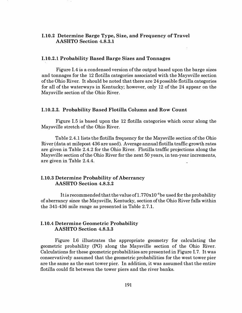
1.10.2 Determine Barge Type, Size, and Frequency of Travel AASHTO Section 4.8.3.1
1.10.2.1 Probability Based Barge Sizes and Tonnages
Figure 1.4 is a condensed version of the output based upon the barge sizes and tonnages for the 12 flotilla categories associated with the Maysville section of the Ohio River. It should be noted that there are 24 possible flotilla categories for all of the waterways in Kentucky; however, only 12 of the 24 appear on the Maysville section of the Ohio River.
1.10.2.2. Probability Based Flotilla Column and Row Count
Figure 1.5 is based upon the 12 flotilla categories which occur along the Maysville stretch of the Ohio River.
Table 2.4.1 lists the flotilla frequency for the Maysville section of the Ohio River (data at milepost 436 are used). Average annual flotilla traffic growth rates are given in Table 2.4.2 for the Ohio River. Flotilla traffic projections along the Maysville section of the Ohio River for the next 50 years, in ten-year increments, are given in Table 2.4.4.
1.10.3 Determine Probability of Aberrancy AASHTO Section 4.8.3.2
It is recommended that the value ofl . 770x10'4be used for the probability of aberrancy since the Maysville, Kentucky, section of the Ohio River falls within the 341-436 mile range as presented in Table 2.7.1 .
1. 10.4 Determine Geometric Probability AASHTO Section 4.8.3.3
Figure !.6 illustrates the appropriate geometry for calculating the geometric probability (PG) along the Maysville section of the Ohio River. Calculations for these geometric probabilities are presented in Figure I. 7. It was conservatively assumed that the geometric probabilities for the west tower pier are the same as the east tower pier. In addition, it was assumed that the entire flotilla could fit between the tower piers and the river banks.
191

1.10.5. Determine Impact Forces AASHTO Sections 3.9, 3.11, 3.12, and 3.14
1.10.5. 1. Probability Based Impact Loads for the Tower Piers
As presented previously in Table 2.3.4, for the Maysville section of the Ohio River, upbound barges operate at only 33% of cargo capacity and travel at maximum absolute velocities (barge transit velocity minus river velocity) of approximately four knots (2.13 m/s, 7 fps, 5 mph). On the other hand, downbound barges travel at 92% of cargo capacity with absolute velocities (barge transit velocity plus river velocity) often knots (5. 18 m/s, 17 fps, 12 mph). Consequently, impact loads and barge counts neglect up bound barge traffic since impact loads from up bound barges are insignificant compared to downbound barges.
Flotilla categories currently using the Maysville section of the Ohio River are given in column 1 of Table I .l . The impact loads, as calculated in Figure II.8, and their associated frequencies are also given in columns 3-5 of Table ! . 1 for the west and east tower piers.
1.10.5.2 Minimum Impact Loads for Tower Piers
As a minimum, the AASHTO Guide Specification requires that all waterway piers, with available water depth equal to the empty draft of a free floating barge, be designed to resist the impact of the empty barge floating with the yearly mean current velocity and elevation at the bridge location. However, the Kentucky Transportation Cabinet has established the more conservative requirement of a single barge, fully loaded, or loaded to a draft equal to the available water depth, drifting at the 100-year current as the design minimum.
The design minimum barge selected for the Maysville section of the Ohio River was a 53-ft x 290-ft barge since it is one of the largest barges currently in use on the river. Barge traffic records indicate 205 downbound passages per year of flotillas with this barge type (see Table 2.4.2 · values for the number of passages per year are halved to account for downbound and up bound trips). The typical dimensions for the 53-ft x 290-ft barge, along with other barge sizes, are given in Table !.2. Calculations for the uniform impact load of a single, fully loaded barge are given in Figure 1.9; the uniform impact load magnitude, length, and bridge pier starting elevations are given in Table 1.3.
192
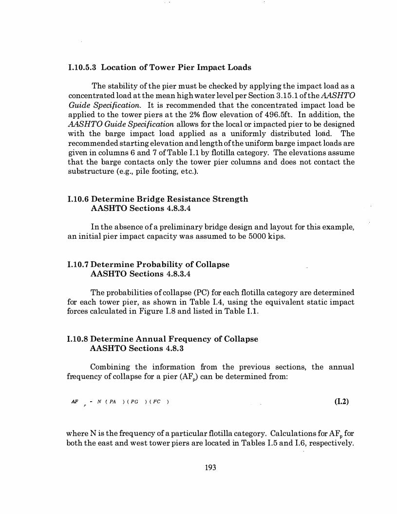
1.10.5.3 Location of Tower Pier Impact Loads
The stability of the pier must be checked by applying the impact load as a concentrated load at the mean high water level per Section 3 .15 .1 of the AASHTO Guide Specification. It is recommended that the concentrated impact load be applied to the tower piers at the 2% flow elevation of 496.5ft. In addition, the AASHTO Guide Specification allows for the local or impacted pier to be designed with the barge impact load applied as a uniformly distributed load. The recommended starting elevation and length of the uniform barge impact loads are given in columns 6 and 7 of Table 1.1 by flotilla category. The elevations assume that the barge contacts only the tower pier columns and does not contact the substructure (e.g., pile footing, etc.).
1.10.6 Determine Bridge Resistance Strength AASHTO Sections 4.8.3.4
In the absence of a preliminary bridge design and layout for this example, an initial pier impact capacity was assumed to be 5000 kips.
1.10.7 Determine Probability of Collapse AASHTO Sections 4.8.3.4
The probabilities of collapse (PC) for each flotilla category are determined for each tower pier, as shown in Table 1.4, using the equivalent static impact forces calculated in Figure 1.8 and listed in Table I .l .
1.10.8 Determine Annual Frequency of Collapse AASHTO Sections 4.8.3
Combining the information from the previous sections, the annual frequency of collapse for a pier (AFP) can be determined from:
AF N ( PA ) ( PG ) ( PC ) ,, (1.2)
where N is the frequency of a particular flotilla category. Calculations for AFP for both the east and west tower piers are located in Tables 1.5 and 1.6, respectively.
193

1.10.9 Determine Design Vessel AASHTO Sections 4.8.2
Based on an initial pier capacity of 5000 kips, the design vessel was determined from the equivalent static impact loads listed in Table 1. 1 to be flotilla category DB impacting the east tower pier.
1.10.10 Determine Bridge Adequacy
After an unacceptable annual frequency of collapse was noted, the initial pier capacity was determined to be inadequate. Therefore, the process was repeated until an impact capacity of7170 kips yielded satisfactory results. Tables 1.7 through 1.9 give the results for the revised calculations. It should be noted that even though the AFP for the east tower pier slightly exceeds the acceptable value of 0.00005, the . summation of the annual frequencies of collapse for all flotilla categories, with respect to both tower piers, is 0.0001. The design vessel for this bridge resistance strength was determined to be flotilla category BC impacting the west tower pier.
1.11 CONCLUSIONS
There is a tremendous variation in the sizes and types of barges and flotillas in use on the Ohio River. Based on the procedures used in this study, there are currently 12 flotilla categories on the Maysville section of the Ohio River. The flotilla sizes and tonnages used to calculate the equivalent static loads for each category have at most a 2.25% chance that a flotilla will pass the Maysville Bridge with greater size or load. Calculations for the equivalent static loads indicated that some categories may be combined since they result in nearly identical impact loads.
Once navigable channel and vessel characteristics have been established, Method II becomes an iterative process whereby an engineer must determine a bridge resistance strength which satisfies the annual frequency of collapse criteria. For this example, a bridge pier capacity of7170 kips, which corresponds to the equivalent static impact force on the west tower pier of flotilla category BC, yielded an acceptable annual frequency of collapse. Again, it should be noted that the information provided in this example is in accordance with the AASHTO Guide Specification; however, it is only intended to illustrate the application of design Method II with the data provided in this study. This example does not constitute a rigorous analysis of the bridge pier design.
194

I t!ct' '"'"" '•H"""'" I I I I I � - - -:J;;O - - - - - - - - - � - - - - - - - - - - - - ''""""'- - - -- - - - - -- -- _lJi!)Ll- - - - - - - - - � ---1 I I ' "'"" ""' I I fl
NOTE: [lf:NIIII·IG l·iOT T<_l ·;,r ALE
I I I I I I I W[",T PIER
I (f'I[R C•)
PLAN
ELEVATIIJN
1 (A',T PIE� I (PIER ,,,
Figure 1.1 : Plan and Elevation Views of the Cable Suspended Bridge Over the Ohio River at Maysville, KY.
195

Set:tinn; )_5 •m<l 4.2 (Swti<Jll 2.5 nfthi" Pupcr)
1.4 Dclc'flninc Vc,...,[ Fled Chur,ctcrislic.; - AASHTO
Soc!iu!\S J.5 and 4.4 (.'\cclitlll.< 2.J un<l 2.4 nflhis ;tndy)
1.7 p,,_.[j, ,oin,·ory Bo·i,kt>' (l,_.·,:i•lll • End lo'iyCHII
1.::: [J,_.t,_., " , ; , , ,_. w.,t.,.,- lkt.th .. -· AA'::HH• ,-'""' t;,,, �-2 ::_·
L ' l [h•t.-' "'iow y,_.._,.,,,_.l 1"'1"" t •l•,_.,_.,·t - AA•:,HTU ·;,,.,_li.:"' 'i_7
(":'""' ti,n ,; r; ,.j thj·_, F'••t•<"l')
�1.-lhoHI II
Figure 1.2: Design Procedure Flow Chart (Modified After AASHTO Guide Specification for Vessel Collision Design of Highway Bridges) .
196

I I
I I I I
I I I
l. Ill. I O.toronino A«'P""'" Crito,;, ibr Ilrid�< C<om!"'nenl; M�,lTO s.,.,tinn 4.H 2 (�\>.{inn 2. H or nO.; •luLl)') !
J
! l ltJ ,, {>rl�''"""' 11011"·" ' F," "'' - /IA':.HTCI ',ro_l<.,r· �.'J, ,) I I , 5 . 1 -', '"''1 J . t J
l I I li t; [lele'm"''' Br�ol,te R�·:�·_,,,_,, � ··,t,�'"tlh AN.HTU "'' lr,_,,, �-1:1 . .3 . 1
! j_ L l
I I I
I I I I I I
I J j
Figure 1.3: Sub Flow Chart Chart for Method II (Modified After AASHTO Guide Specification for Vessel Collision Design of Highway Bridges) .
197
I
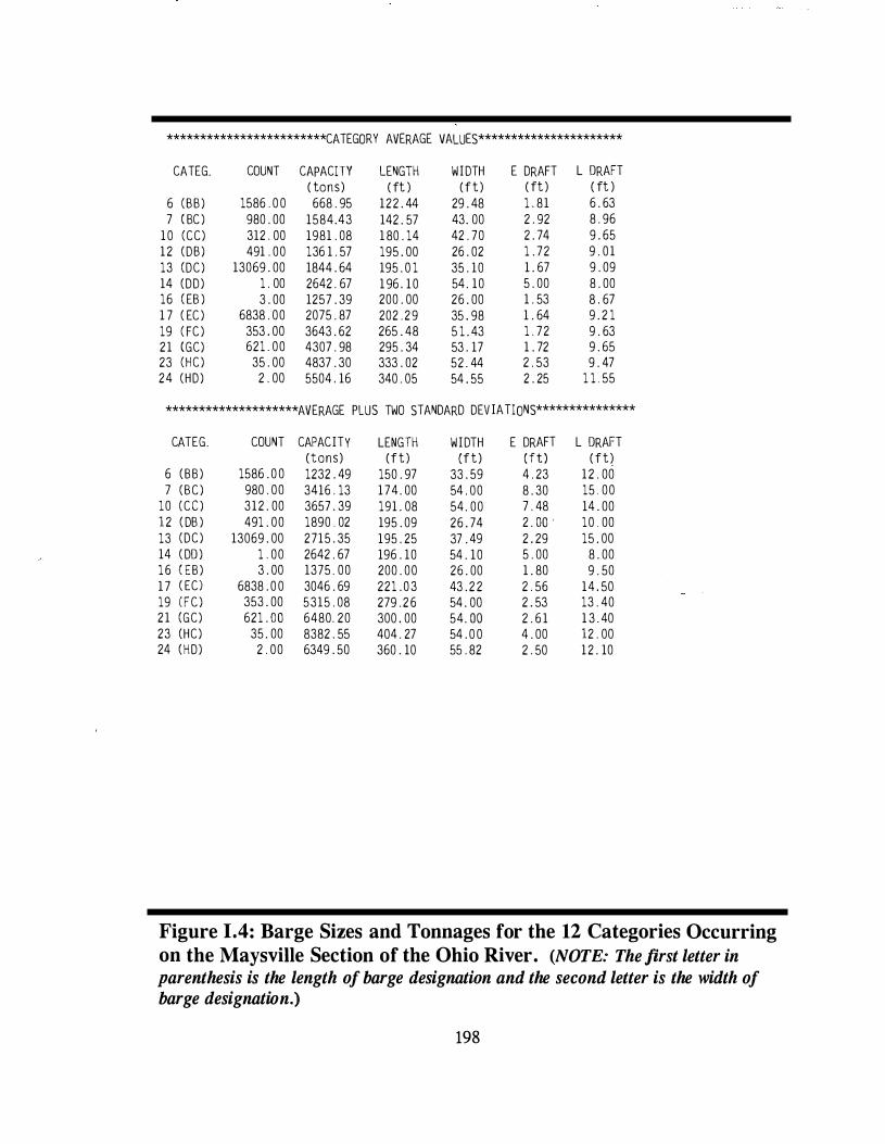
************************CATEGORY AVERAGE VALUES**********************
CATEG.
6 CBB) 7 C BC )
1 0 CCC) 1 2 (DB) 13 (DC) 14 (DD) 16 ( EB ) 1 7 ( EC ) 19 C FC ) 2 1 CGC) 23 CHC) 24 (HD)
COUNT CAPACITY ( tons)
1586 . 0 0 668 . 95
980 . 00 1584.43
312 . 00 1981 . 08
491 . 00 136 1 . 57
13069 . 00 1844 . 64
1 . 00 2642 . 67
3 . 00 1257 . 39
6838 . 00 2075 . 87
353 . 00 3643 . 62
621 . 00 4307 . 98
35 . 00 4837 . 30
2 . 00 5504 . 16
LENGTH W I DTH E DRAFT L DRAFT
( ft ) (ft) ( ft) ( ft ) 122 . 44 29 . 48 1 . 81 6 . 63
142 . 57 43. 00 2 . 92 8 . 96
1 80 . 14 42 . 70 2 . 74 9 . 65
195 . 00 26 . 02 1 . 72 9 . 0 1
195 . 0 1 35 . 10 1 . 67 9 . 09
1 96 . 1 0 54. 10 5 . 00 8 . 00
200 . 00 26 . 00 1 . 53 8 . 67
202 . 2 9 35 . 98 1 . 64 9 . 2 1
265 . 48 5 1 . 43 1 . 72 9 . 63
295 . 34 53 . 17 1 . 72 9 . 65
333 . 02 52 . 44 2 . 53 9 . 47
340 . 05 54 . 55 2 . 25 1 1 . 55
********************AVERAGE PLUS TWO STANDARD DEV IATIONS***************
CATEG.
6 (BB) 7 (BC)
10 CCC) 1 2 ( DB ) 13 CDC) 14 ( DD ) 1 6 ( EB) 1 7 ( ECl 19 CFC) 2 1 (GC) 23 (HC) 24 (HD)
COUNT
1586 . 0 0
980 . 00
312 . 00
491 . 00
13069 . 00
1 . 00
3 . 00
6838 . 0 0
353 . 00
621 . D O 35 . 00
2 . 00
CAPACITY (tons) 1232 . 49
3416 . 13
3657 . 39
1890 . 02
2715 . 35
2642 . 67
1375 . 00
3046 . 69
5315 . 08
6480. 20
8382 . 55
6349 . 50
LENGTH W I DTH E DRAFT L DRAFT (ft) (ft) (ft) ( ft)
150 . 97 33 . 59 4 . 23 1 2 . 00
174. 00 54 . 00 8 . 30 15 . 00
191 . 08 54. 00 7 . 48 14 . 00
195 . 09 26 . 74 2 . DO · 10 . 00
195 . 25 37 . 49 2 . 29 15 . 00
196 . 10 54 . 10 5 . 00 8 . 00
200 . 00 26 . 00 1 . 80 9 . 50
221 . 0 3 43 . 2 2 2 . 56 14 . 50
279 . 2 6 54 . 00 2 . 53 13 . 40
300 . 00 54. DO 2 . 6 1 1 3 . 40
404 . 27 54 . 0 0 4 . 00 12 . 00
360 . 10 55 . 82 2 . 50 1 2 . 10
Figure 1.4: Barge Sizes and Tonnages for the 12 Categories Occurring on the Maysville Section of the Ohio River. (NOTE: The first letter in
parenthesis is the length of barge designation and the second letter is the width of barge designation.)
198
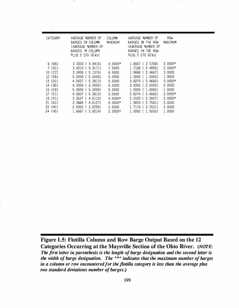
CATEGORY AVERAGE NUMBER OF COLUMN AVERAGE NUMBER OF ROW BARGES I N COLUMN MAXIMUM BARGES IN THE ROW MAX I MUM ( AVERAGE NUMBER OF (AVERAGE NUMBER OF BARGES IN COLUMN BARGES I N THE ROW PLUS 2 STD OEVs) PLUS 2 STD DEVs)
6 ( B B ) 3 . 3333 ( 5 . 4415) 4 . 0000* 1 . 6667 ( 2 . 7 208) 2 . 0000*
7 ( 8C) 3 . 4219 ( 5 . 91 7 1 ) 7 . 5000 1 . 7188 ( 2 . 4995) 2 . 0000*
10 ( cc) 3 . 3490 ( 5 . 1076) 6 . 5000 1 . 9688 ( 2 . 4667) 3 . 0000 12 ( D B ) 5 . 0000 ( 5 . 0000) 5 . 0000 1 . 0000 ( 1 . 0000) 1 . DODO 13 (DC) 4 . 5837 ( 5 . 3813) 5 . 5000 2 . 8274 ( 3 . 4682) 3 . 0000* 14 ( DO ) 6 . 0000 ( 6 . 0000 ) 6 . 0000 2 . 0000 ( 2 . 0000) 2 . 0000 16 ( E B ) 5 . 0000 ( 5 . 0000) 5 . 0000 1 . 0000 ( 1 . 0000 ) 1 . 0000 17 lECl 4 . 5837 ( 5 . 3813) 5 . 5000 2 . 8274 ( 3 . 4682) 3 . 0000* 19 ( FC ) 3 . 3537 ( 4 . 6113) 4 . 5000* 2 . 3159 ( 3 . 3007) 3 . 0000* 21 (GC) 3 . 3884 ( 4 . 6127) 4 . 0000* 1 . 9876 ( 2 . 7581) 3 . 0000 23 ( HC) 2 . 0000 ( 3 . 2295) 3 . 5000 1 . 7176 ( 2 . 7621) 3 . 0000 24 ( HO ) 1 . 6667 ( 2 . 8214) 2 . 0000* 1 . 0000 ( 1 . 0000) 1 . 0000
Figure 1.5: Flotilla Column and Row Barge Output Based on the 12 Categories Occurring at the Maysville Section of the Ohio River. (NOTE:
The first letter in parenthesis is the length of barge designation and the second letter is the width of barge designation. The "*" indicates that the maximum number of barges in a column or row encountered for the flotilla category is less than the average plus two standard deviations number of barges.)
199

d
d 2
l l i L I = U\L\
Figure 1.6: Dimensions for the Calculation of Geometric Probability for the Maysville Section of the Ohio River.
200
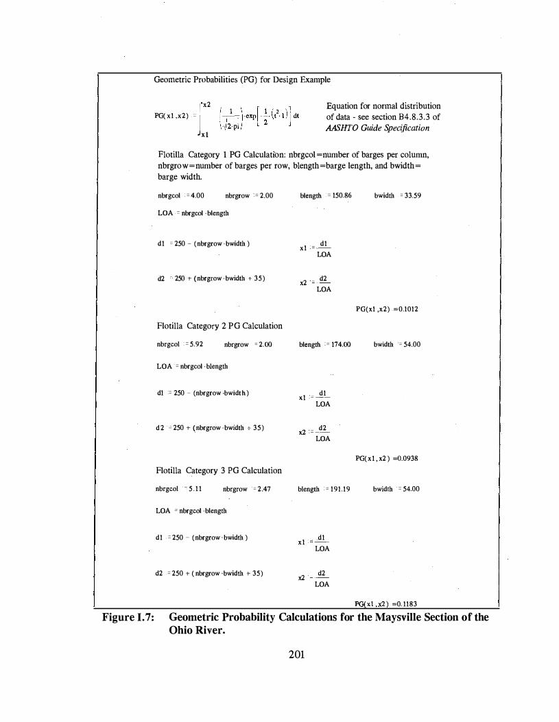
Figure 1.7:
Geometric Probabilities (PG) for Design Example
PG( x1 ,x2) _
l'x2
l Equation for normal distribution
of data - see section B4.8.3.3 of
MSHTO Guide Specification
Flotilla Category I PG Calculation: nbrgcol �number of barges per column,
nbrgrow�number of barges per row, blength�barge length, and bwidth�
barge width.
nbrgcol = 4.00 nbrgrow = 2.00
LOA = nbrgcol · blength
d 1 = 250 - ( nbrgrow · bwidth )
d2 250 + ( nbrgrow · bwidth + 35)
Flotilla Category 2 PG Calculation
nbrgcol : = 5.92 nbrgrow = 2.00
LOA -= nbrgcol · blength
d1 := 250 - (nbrgrow ·bwidth)
d2 ·--" 250 + ( nbrgrow · bwidth -:-- 35)
Flotilla Category 3 PG Calculation
nbrgcol · ---: 5 . 1 1 nbrgrow = 2.47
LOA = nbrgcol · blength
d 1 - = 250 - ( nbrgrow · bwidth )
d2 = 250 + ( nbrgrow · bwidth + 35)
blength c 150.86
x1 d1
LOA
x2 - d2
LOA
blength := 174.00
x1 d1 .- --
LOA
x2 - d2
LOA
blength · = 191.19
x1
x2
d1
LOA
d2
LOA
bwidth = 33.59
PG(x1 ,x2) �0.1012
bwidth ·= 54.00
PG(x1 , x2 ) �.0938
bwidth · = 54.00
PG(x1 ,x2) �0. 1183
Geometric Probability Calculations for the Maysville Section of the Ohio River.
201

Flotilla Category 4 PG Calculation
nbrgcol c 5. 00 nbrgrow " 1 . 00 blength = 195.09 bwidth = 26.74
LOA = nbrgcol · blength
x1 d1
- -d1 = 250 - ( nbrgrow · bwidth )
LOA
x2 d2 - - -d2 . = 250 1- ( nbrgrow · bwidth + 35 )
LOA
PG(x1 ,x2) :o{).0348
Flotilla Category 5 PG Calculation
nbrgcol = 5.38 nbrgrow = 3. 00 blength = 195.25 bwidth = 37.49
LOA = nbrgcol · blength
x1 d1
- ·-d l = 250 .. (nbrgrow · bwidth )
LOA
x2 d2
-d2 = 250 + ( nbrgrow · bwidth + 35)
LOA
PG(xl ,x2) :o{).0953
Flotilla Category 6 PG Calculation
nbrgcol = 6.00 nbrgrow = 2.00 blength : = 196.10 bwidth = 54.10
LOA = nbrgcol · blength
x1 d1
- --� d1 = 250 - ( nbrgrow · bwidth )
LOA
x2 d2 - ----d2 = 250 ,. (nbrgrow · bwidth + 35 )
LOA
PG(x1 ,x2) :o{).0829
Figure I. 7 (continued): Geometric Probability Calculations for the Maysville Section of the Ohio River.
202

Flotilla Category 7 PG Calculation
nbrgcol = 5.00 nbrgrow = I. 00
LOA = nbrgcol · blength
d l = 250 - ( nbrgrow · bwidth )
d2 = 250 + ( nbrgrow · bwidth + 35 )
Flotilla Category 8 PG Calculation
nbrgcol = 5.38 nbrgrow = 3. 00
LOA . = nbrgcol · blength
dl = 250 - ( nbrgrow · bwidth )
d2 = 250 + ( nbrgrow · bwidth + 35 )
Flotilla Category 9 PG Calculation
nbrgcol = 4.50 nbrgrow := 3.00
LOA · = nbrgcol · blength
dl = 250 - ( nbrgrow · bwidth )
d2 := 250 ,_ ( nbrgrow · bwidth + 35 )
blength = 200.00
xl dl
LOA
d2 x2 - --
LOA
blength = 221 .03
x l dl - --
LOA
x2 d2 - --
LOA
blength : = 279.26
xl dl - -·-
LOA
x2 d2 - -
LOA
bwidth = 26.00
PG(xl ,x2) =0.0335
bwidth = 43.23
PG(x l ,x2) =0.0961
bwidth = 54.00
PG(xl , x2 ) =0. 1 1 1 1
Figure 1.7 (continued): Geometric Probability Calculations for the Maysville Section of the Ohio River.
203
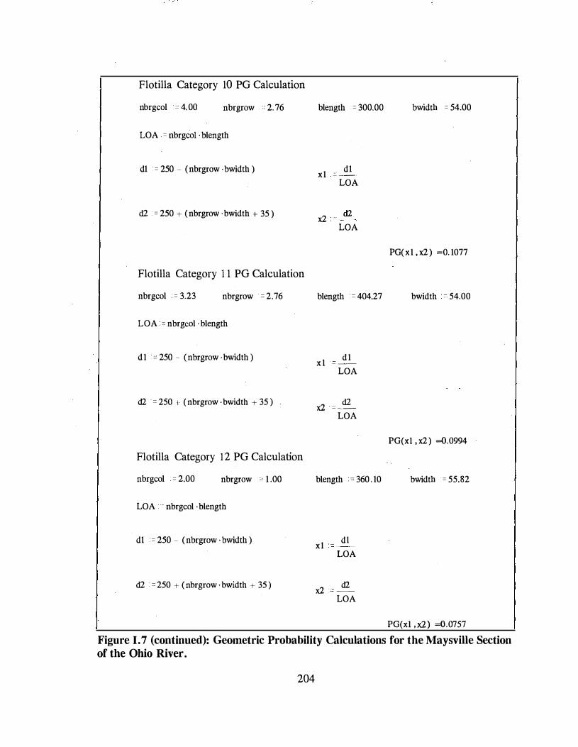
Flotilla Category 10 PG Calculation
nbrgcol = 4. 00 nbrgrow = 2. 76 blength = 300.00 bwidth = 54.00
LOA = nbrgcol · blength
x1 d1
- --d1 = 250 - ( nbrgrow · bwidth )
LOA
d2 • = 250 + ( nbrgrow · bwidth + 35 ) x2 d2 LOA
PG( x1 , x2 ) =0. 1077
Flotilla Category 1 1 PG Calculation
nbrgcol = 3.23 nbrgrow = 2. 76 blength = 404.27 bwidth = 54.00
LOA = nbrgcol · blength
x 1 d1
- --d1 = 250 - ( nbrgrow · bwidth )
LOA
x2 d2 - --
d2 = 250 + ( nbrgrow · bwidth + 35 )
LOA
PG(x1 , x2 ) =0.0994
Flotilla Category 12 PG Calculation
nbrgcol = 2.00 nbrgrow • 1 .00 blength = 360 . 10 bwidth = 55.82
LOA - nbrgcol · blength
x1 dl
- --d 1 = 250 - ( nbrgrow · bwidth )
LOA
x2 d2 - -
d2 = 250 + ( nbrgrow · bwidth + 35 )
LOA
PG(x1 , x2 ) =0.0757
Figure 1.7 (continued): Geometric Probability Calculations for the Maysville Section of the Ohio River.
204

THE MAYSVILLE KENTUCKY BRIDGE OVER THE OHIO RIVER
BARGE EQUIVALENT STATIC IMPACT FORCE CALCULATIONS
Barge Design Impact Velocity West Pier: Barge Transit V = 10.27 fps (7.00 mph)
Waterway V =5.7 fps (3.89 mph)
v w o ( 10.27 + 5.7) (fps)
Barge Design Impact Velocity East Pier: Barge Transit V= 10.27 fps (7.00 mph)
Waterway V = 6. 1 fps ( 4 . 1 5 mph)
V E 0 ( 10.27 + 6. 1 ) (fps)
Hydrodynamic Coefficient
Individual Barge Displacement (tons): By barge type, i = 1 ,2, . . . ,24.
Tli defines the 97.75 percentile barge tonnages.
TI1 o 633
TI, o 953
TJ, o 4486
TI4 o 50!
TI5 o 1433
TI6 o 1232
TL, c 3416
TJ, o 1868
TI10 o 3657
TI1 1 o 421
TI12 o 1890
TI13 o 2715
T!l4 ° 2643
T!IS " I !56
T!l7 " 3047
TJ18 c 77J4
TI19 o 5315
�O c 426J
TI,1 o 6480
TI, 0 7497
TI,3 " 8383
TJ, c 3664 TI16 o 1375 T� o 6350
Figure 1.8: Barge Equivalent Static Impact Force Calculations for the Maysville Section of the Ohio River.
205
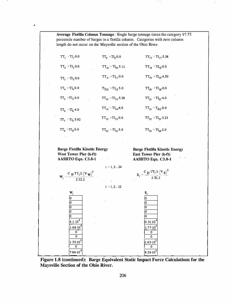
.
Average Flotilla Column Tonnage : Single barge tonnage times the category 97.75 percentile number of barges in a flotilla column. Categories with zero column
length do not occur on the Maysville section of the Ohio River.
TTl c TlrO.O TT9 = Tlg·OcO
TT2 = TL,·O.O TT10 = TI10·5 . 1 1
TT, = TJ,·O.O TT11 =TI1 1·0.0
TT4 = n4o.o TT12 =TI12·5.0
TT5 =n,.o.o TT13 =TI13·5.38
TT6 = TI04.0 TT14 = TI146.0
TT, =TI7·5.92 TT15 =TI15o.o
TT, =n8o.o TT16 = TI105.0
Barge Flotilla Kinetic Energy West Tower Pier (k-ft) AASHTO Eqn. C3.8-1
( • 2 _ c a·TTr2· v wJ
w --- ---.. ---' 2·32.2
w, 0 0 0 0 0 4.1 · 104 1 .68·105
0 0
1 .55·105 0
7.86·104
i = 1 ,2 .. 24
i = 1 ,2 . . 12
TT17 = TI17·5.38
TTl a = Tli80.0
TT19 = TI19·4.50
TT20 = TI,o·O.O
TTz! = Tlzr4.o
TTzz = TlziO.O
TT23 = TL,,-3.23
TT24 = Tlz42.0
Barge Flotilla Kinetic Energy East Tower Pier (k-ft) AASHTO Eqn. C3.8-1
0 0 0 0 0 4.31·104
1.77-105 0 0
1.63·105
0 8.26·104
Figure 1.8 (continued): Barge Equivalent Static Impact Force Calculations for the Maysville Section of the Ohio River.
206

i = 13 . . 24 w ; E ; 1.21·105 1.28·105
1.32·105 1.39·105
0 0 5.72·104 6.01·104
1.36·105 1.43·105
0 0 1.99·105 2.09· 105
0 0 2.16·105 2.26·105
0 0 2.25·105 2.37·105
1.06·105 1 . 11 · 105
Barge Width Correction Factors: Using the Most Conservative Width in the Flotilla Category (pe1· AASHTO definition R = ratio of barge width to 35-ft.)
- 25.70 R1 35
- 33.13 R2 35
R = �:00 3 35
R = 55.00 4 35
Rs - 25.00
35
R = 33.59 6 35
R = 54.00 7 35
- 59.30 R, 35
= 26,98 R, 35
R = 54.<JO_ 10 35
R = (jO.OO II 35
- 26.74 R12 35
R = 37.49 13 . 35
R , 54.00 14 35
- 25.00 R1s 35
R = 26.00 16 35
R = 43:23 17 35
R = 72.00 18 35
R19 - 54.00
35
R =_62.69 20 35
R = 54.0() 21 35
R = 56,64 22 35
R = 54.00 23 35
R,4 - 55.82
35
Figure 1.8 (continued): Barge Equivalent Static Impact Force Calculations for the Maysville Section of the Ohio River.
207
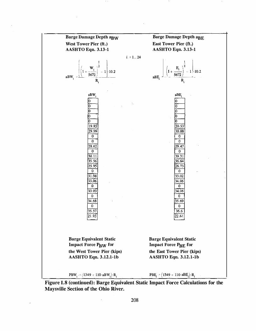
Barge Damage Depth aBw West Tower Pier (ft.) AASHTO Eqn. 3.13-1
1 ; w. �� j : I I L I \ I + - -1 - I · 10.2
aBW, = _L -·· 5672 1.. -- -R,
Barge Equivalent Static Impact Force I'JJw for
the West Tower Pier (kips) AASHTO Eqn. 3.12.1-1b
PBW, = (1349 1 1 10-aBW,)-R,
i = 1 . . 24
Barge Damage Depth aBE East Tower Pier (ft.) AASHTO Eqn. 3.13-1
I
aBE J�+S�J I · 10.2 ' R '
Barge Equivalent Static Impact Force I'JJE for
the East Tower Pier (kips) AASHTO Eqn. 3.12. 1-1b
PBE = ( 1349 + llO ·aBE_) ·R ' ' '
Figure 1.8 (continued): Barge Equivalent Static Impact Force Calculations for the Maysville Section of the Ohio River.
208
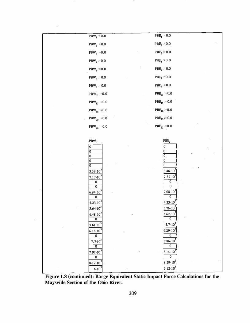
PBW1 =0.0
PBW2 = 0.0
PBW3 =0.0
PBW4 =0.0
PBW5 =0.0
PBW8 = 0.0
PBW9 = 0.0
PBW11 =0.0
PBW15 = 0.0
PBW18 = 0.0
PBW20 = 0.0
PBW22 = 0.0
0 0 0 0 3.39· 103
7.17·103 0 0
6.94· w' 0
4.23· w'
5.64·103
6.48· w' 0
3.61· w'
6.16· w' 0
7.7·103 0
7.97 · 103 0
8.12·103
6·103
PBE1 = 0.0
PBEz = 0.0
PBE, = 0.0
PBE4 =0.0
PBE5 = 0.0
PBEg =0.0
PBJ;, = 0.0
PBE, 1 = 0.0
PBE15 = 0.0
PBE18 =0.0
PBEz0 = 0.0
PBEz2 =0.0
PBF, 0 0 0 0 0 3.46· w'
7.32·103 0 0
7.08· w' 0
4.33· w'
5.76 · 103
6.62· w' 0
3.7· w'
6.29· 103 0
7.86· w' 0
8.14· w' 0
8.29· 103
6.12·103
Figure 1.8 (continued): Barge Equivalent Static Impact Force Calculations for the Maysville Section of the Ohio River.
209
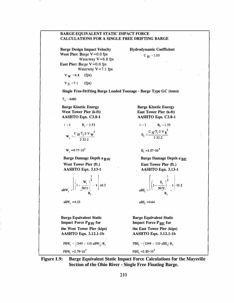
BARGE EQUIVALENT STATIC IMPACT FORCE CALCULATIONS FOR A SINGLE FREE DRIFTING BARGE
Barge Design Impact Velocity West Pier: Barge V =0.0 fps
Waterway V =6 . 8 fps East Pier: Barge V = 0. 0 fps
Waterway V =7. 1 fps
v w = 6.8 (fps)
v E=7.1 (fps)
Hydrodynamic Coefficient
C H = 1.05
Single Free-Drifting Barge Loaded Tonnage - Barge Type GC (tons):
T1 = 6480
Barge Kinetic Energy West Tower Pier (k-ft) AASHTO Eqn. C3.8-1
R, = 1.53
2 C H·T,-2·Y w w. = ------' 2·32.2
w, =9.77• 103
Barge Damage Depth a BW West Tower Pier (ft.) AASHTO Eqn. 3.13-1
aBW, =4.33
Barge Equivalent Static Impact Force PBW for
the West Tower Pier (kips) AASHTO Eqn. 3.12.1-1b
PBW1 = (1349 c 110·aBW,) ·R,
PBW, =2.79 · 103
Barge Kinetic Energy East Tower Pier (k-ft) AASHTO Eqn. C3.8-1
Barge Damage Depth a· BE East Tower Pier (ft.) AASHTO Eqn. 3.13-1
l , E. )� ( 1 +-' . - 1 · 10.2 - . 5672 , aBEi R,
aBE1 =4.64
Barge Equivalent Static Impact Force PBE for
the East Tower Pier (kips) AASHTO Eqn. 3.12.1-1b
PBE, = ( 1349 c· l lO·aBE,) ·R,
PBE1 =2. 85 · 103
Figure 1.9: Barge Equivalent Static Impact Force Calculations for the Maysville Section of the Ohio River - Single Free Floating Barge.
210
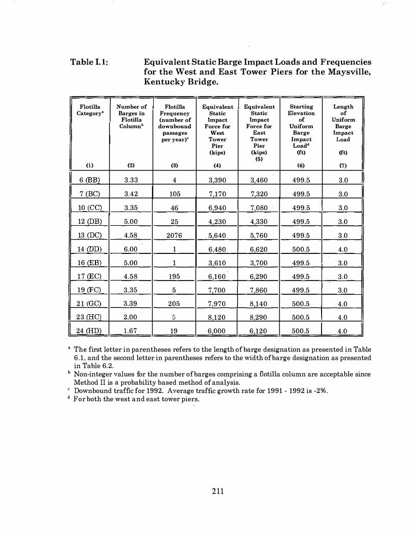
Table I. I:
Flotilla Category"
(1)
6 (BB)
7 (BC)
10 (CC)
12 (DB)
13 (DC)
14 (DD)
16 (EB)
17 (EC)
19 (FC)
21 (GC)
23 (HC)
24 (HD)
Equivalent Static Barge Impact Loads and Frequencies for the West and East Tower Piers for the Maysville, Kentucky Bridge.
Number of Flotilla Equivalent Equivalent Starting Length Barges in Frequency Static Static Elevation of
Flotilla (number of Impact Impact of Uniform Columnh down bound Force for Force for Uniform Barge
passages West East Barge Impact per year)" Tower Tower Impact Load
Pier Pier Loadd (kips) (kips) (ft) (ft)
(5) (2) (3) (4) (6) (7)
3.33 4 3,390 3,460 499.5 3.0
3.42 105 7,170 7,320 499.5 3.0
3.35 46 6,940 7,080 499.5 3.0
5.00 25 4,230 4,330 499.5 3.0
4.58 2076 5,640 5,760 499.5 3.0
6.00 1 6,480 6,620 500.5 4.0
5.00 1 3,610 3,700 499.5 3.0
4.58 195 6,160 6,290 499.5 3.0
3.35 5 7,700 7,860 499.5 3.0
3.39 205 7,970 8,140 500.5 4.0
2.00 5 8,120 8,290 500.5 4.0
1.67 19 6,000 6,120 500.5 4.0
' The first letter in parentheses refers to the length of barge designation as presented in Table 6.1 , and the second letter in parentheses refers to the width of barge designation as presented in Table 6.2.
• Non-integer values for the number of barges comprising a flotilla column are acceptable since Method II is a probability based method of analysis.
' Downbound traffic for 1992. Average traffic growth rate for 1991 - 1992 is -2%. d For both the west and east tower piers.
211

Table 1.2: Typical Barge Size Dimensions.
Length, LR
Width, BM
Depth, Dv
Em11ty Draft, D.
Loaded Draft, D,.
Depth of Bow, Dn
Bow Rake Lenl':th, R
Head Lo11: Height, H
Cargo Weight, C,
Empty Weight, WE
Total Weight, WL
(ft) 195
(ft) 35
(ft) 12
(ft) 1.7
(ft) 8.7
(ft) 13
jft) 20
_(ft) 2·3
(tons .1700 )
(tons 200 )
(tons 1900 )
Length ( L [l )
PLAN
_______ ,..._ Direction of Travel
I 1 '
290
53
12
1. 7
8 .7
13
25
2-3
3700
600
4300
, H :------------�--------------'� [• t'··"·"'""l Lir·· . i l i { [I ) L I •
ELEVATION
212
250
72
17
2.5
12.5
18
30
3·5
5000
1300
6300
H f , _ _
[\

Table 1.3: Equivalent Static Impact Loads for the West and East Tower Piers for a Single Free Floating 53-ft x 290-ft Barge.
Uniform Barge Uniform Equivalent Equivalent Impact Load Barge Static Impact Static Impact
Starting Impact Load Force Force Elevation Length West Pier East Pier
(ft) (ft) (kips) (kips)
(1) (2) . (3) (4)
500.5 4.0 2,790 2,850
213

Table 1.4: Probability of Collapse for the Maysville Bridge (HP = 5000 kips).
HJP,' Probability of Collapseh Category
East Pier West Pier East Pier West Pier
6 (BB) 1.4451 1.4749 0.0000 0.0000
7 (BC) 0.6831 0.6974 0.0352 0.0336
10 iCC) 0.7062 0.7205 0.0326 0.0311
12 (DB) 1. 1547 1.1820 0.0000 0.0000
13 (DC) 0.8681 0.8865 0.0147 0.0126
14 (DD) 0. 7553 0.7716 0.0272 0.0254
16 (EB) 1.3514 1.3850 0.0000 0.0000
17 (EC) 0.7949 0.8117 0.0228 0.0209
19 (FC) 0.6361 0.6494 0.0404 0.0390
21 (GC) 0.6143 0.6274 0.0429 0.0414
23 (HC) 0.6031 0.6158 0.0441 0.0427
24 (HD) 0.8170 0.8333 0.0203 0.0185
' H. is the pier capacity and P, is the equivalent static load for each flotilla category as found in Table II. l .
b The Probability of Collapse is calculated as: PC = (1-H,IP,)/9 for 0 .1 :S H,IP, :S 1.0. PC = 0 for Il.IP, > 1.0.
214
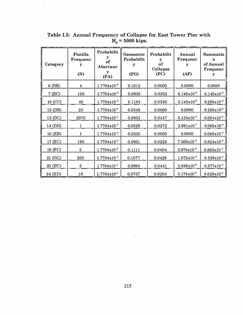
Table 1.5: Annual Frequency of Collapse for East Tower Pier with � = 5000 kips.
Flotilla Probabilit Geometric Probabilit Annual Summatio Frequenc y Probabilit y Frequenc n
of Category y Aberranc y of y of Annual Collapse Frequenc
(N) y (PG) (PC) (AF) y (PA)
6 (BB) 4 1.7704x1o·• 0.1012 0.0000 0.0000 0.0000
7 (BC) 105 1.7704x1o·• 0.0938 0.0352 6. 140x10·' 6.140x1o·'
10 (CC) 46 1. 7704x1o·• 0 .1183 0.0326 3.145xl0"5 9.285x1o·'
12 (DB) 25 1. 7704x1o·• 0.0348 0.0000 0.0000 9.285x1o·'
13 (D_C) 2076 1.7704x1o·• 0.0953 0.0147 5.135x10"4 6.064x1o·•
14Q:JD) 1 1 . 7704xl0·4 0.0829 0.0272 3.991x10.7 6.068xl0"4
16 (EB) 1 1 . 7704x1o·' 0.0335 0.0000 0.0000 6.068x1o·•
17 (EC) 195 1. 7704x1o·• 0.0961 0.0228 7.560x10·5 6.824x1o·•
19 (FC) 5 1 . 7704x1o·• 0 .1111 0.0404 3.976x10"6 6.863x1o·'
21 (GC) 205 1. 7704x1o·' 0.1077 0.0429 1.675x10·' 8.539xl0·4
23 QIC) 5 1. 7704xl0"4 0.0994 0.0441 3.880x1o·• 8.577x1o·'
24 (HD) 19 1 . 7704xl0·' 0.0757 0.0203 5.178xl0"6 8.629xl0·4
215
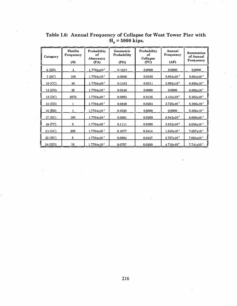
Table 1.6: Annual Frequency of Collapse for West Tower Pier with HP == 5000 kips.
Flotilla Probability Geometric Probability Annual Summation
Category Frequency of Probability of Frequency
of Annual Aberrancy Collapse
Frequency (N) (PA) (PG) (PC) (AF)
6 (BB) 4 1. 7704xlo··l 0.1012 0.0000 0.0000 0.0000
7 (BC) 105 1 .7704xtO··• 0.0938 0.0336 5.864xl0·5 5.864xlO.r,
10 (CC) 46 1 .7704x10'' 0.1183 0.031 1 2.992xlO.r; 8.856x1o··•
12 (DB) 25 1.7704x10"1 0.0348 0.0000 0.0000 8.856xl0''
13 (DC) 2076 1.7704xl0"'1 0.0953 0.0126 4.41Gx10"'1 5.302xlo··l
14 (DD) 1 1.7704x10"' 0.0829 0.0254 3.725x10'' 5.306x10''
16 (EB) 1 1.7704x1o·' 0.0335 0.0000 0.0000 5.306xlo··'
17 (EC) 195 1. 7704xto·� 0.0961 0.0209 6.942xlO.r, 6.000x10"'1
19 (FC) 5 1.7704x10"' 0.1 1 1 1 0.0390 3.832x10"11 6.038x10"'1
2 1 (GC) 205 1.7704x10"' 0. 1077 0.0414 1.618xl0"'1 7.657xl0""1
23 (HC) 5 L7704xlo··l 0.0994 0.0427 3.757xlO.n 7.694xto·�
24 (HD) 19 1 .7704xl0""1 0.0757 0.0200 4. 716x10"6 7.74lx10"'1
216

Table I. 7: Probability of Collapse for the Maysville Bridge (H. = 7170 kips).
H,fP, Probability of Collapse• Category
East Pier West Pier East Pier West Pier
6 (BB� 2.0723 2.1150 0.0000 0.0000
7 (BC) 0.9795 1.0000 0.0023 0.0000
10 (CC) 1.0127 1.0331 0.0000 0.0000
12 (DB) 1.6559 1.6950 0.0000 0.0000
13 (DC) 1.2448 1.2713 0.0000 0.0000
14 (DD) 1.0831 1.1065 0.0000 0.0000
16 (EB) 1.9378 1.9861 0.0000 0.0000
17 (EC) 1 . 1399 1 .1640 0.0000 0.0000
19 (FC) 0.9122 0.9312 0.0098 0.0076
21 (GC) 0.8808 0.8996 0.0132 0.0112
23 fr[C) 0.8649 0.8830 0.0150 0.0130
24 (l!D) 1 .1716 1 .1950 0.0000 0.0000
217

Table 1.8: Annual Frequency of Collapse for East Tower Pier with HP = 7170 kips.
Flotilla Probability Geometric Probability Annual Summation
Category Frequency of Probability of Frequency
of Annual Aberrancy Collapse
Frequency (N) (PA) (PG) (PC) (AF)
6 (BB) 4 1.7704xm' 0.1012 0.0000 0.0000 0.0000
7 (BC) 105 !.7704xm' 0.0938 0.0023 3.970xl0·" 3.970x10""
10 (CC) 46 I. 7704xl0 ·' 0 . 1 183 0.0000 0.0000 3.970x10·!;
12 (DB) 25 1 .7704x10··• 0.0348 0.0000 0.0000 3.970xl0.r,
13 (DC) 2076 1.7704x10·' 0.0953 0.0000 0.0000 3.970xl0.r,
14 (DD) 1 ! .7704x1o··• 0.0829 0.0000 0.0000 3.970xlO.n
16 (EB) 1 !.7704x10·' 0.0335 0.0000 0.0000 3.970x10.n
17 (EC) 195 1.7704x10·"1 0.0961 0.0000 0.0000 3.970xl0·6
19 (FC) 5 1.7704x10·'1 0. 1 111 0.0098 9.593x10·? 4.929xl0"11
21 (GC) 205 1 . 7704x10""' 0.1077 0.0132 5.175x1Q·� 5.668x10"'
23 (HC) 5 L7704x10'4 0.0994 0.0150 1.321xl0'/J 5.800xlO.r,
24 (HD) 19 1.7704xl0 .. 1 0.0757 0.0000 0.0000 5.800x10'1;
218

Table 1.9: Annual Frequency of Collapse for West Tower Pier with Hp = 7170 kips.
Flotilla Probability Geometric Probability Annual Summation
Category Frequency of Probability of Frequency
of Annual Aberrancy Collapse
Frequency (N) (PA) (PG) (PC) (AF)
6 (BB) 4 1. 7704xlo·• 0. 1012 0.0000 0.0000 0.0000
7 (BC) 105 1 .7704xt0·'1 0.0938 0.0000 0.0000 0.0000
10 (CC) 46 L7704x10"4 0.1 183 0.0000 0.0000 0.0000
12 (DB) 25 1.7704x10"'1 0.0348 0.0000 0.0000 0.0000
13 (l)C) 2076 1. 7704xto··l 0.0953 0.0000 0.0000 0.0000
14 (DD) I 1.7704xl0"'1 0.0829 0.0000 0.0000 0.0000
16 (EB) I 1.7704x!O"'' 0.0335 0.0000 0.0000 0.0000
17 (EC) !95 1. 7704xto··l 0.0961 0.0000 0.0000 0.0000
19 (FC) 5 1.7704xl0 .. 1 0. 1 1 1 1 0.0076 7.52 lxl0·7 7.521xt0·7
2! (GC) 205 1.7704x!O"'' 0.1077 0.0112 4.359xJo·' 4.435x!O""
23 (HC) 5 I. 7704x!O"'' 0.0994 0.0130 L 144x10.u 4.549xJO·"
24 (HD) 19 1.7704x10·4 0.0757 0.0000 0.0000 4.549xiO·'
219

APPENDIX II. SOLUTION METHOD FOR CONVOLUTION INTEGRAL
The method used to solve Eqn. 3.40 used in the derivation of the impact spectrums given in Section 3 is given here. Eqn. 3.40 is written as
u. ( t ) = [ A ( t ) sin w t - B ( t ) cos w t ] n o
where
A ( t )
B ( t )
I ' ' ' " ' --
p ( < ) -- cos w 't" d "t"
m w f u e { "' 1
m w f u
' ' ' " '
p ( • ) -- sin ' " ' '
w 1" d 1"
(II.42)
(Il.43a)
(II.43b)
Writing Eqns. II.43 in their recursive form and using Simpson's rule to integrate gives
F ( t . ) F ( t b.
' [ --- " ' ' " " y ' . '
3 m w D
Y1
"' p ( t ) cos wD
for F ( t ) • A ( t )
y 1" p ( t ) sin w
n
where and
for F ( t ) • B ( t )
F ( t . ) A ( t for A ( t )
F ( t . ) B ( t . ) for B ( t )
- 2 � "' tl I l 4 y e + y I · I (11.44)
(11.45a) (11.45b)
(II.46a) (11.46b)
After calculating the values of A(t) and B(t) for succesive values of �. the displacement at time ti is calculated using
(II.47)
220

APPENDIX III. IMPACT SPECTRUM ANALYSIS PROCEDURE (MULTIPLE INERTIAL MODE PROCEDURE)
III.l INTRODUCTION
The purpose of this appendix is to propose a second analysis procedure as a modification to the current AASHTO Guide Specification equivalent static design procedure by including the dynamic effects of multiple inertial modes. The need for a multiple mode method is based on a type of common inland waterway bridge pier with a significant concentrated mass at an intermediate point along the height of the pier that could result in significant higher mode displacement contribution. This pier type is depicted in Figure III .l .l . It is obvious for this type of structure that more than one inertial mode may significantly contribute to the total impact response of the structure.
The Impact Spectrum Analysis Procedure (ISAP) given in this Section uses a multi-inertial mode analysis technique which, for simplicity in this appendix, is assumed to have two inertial modes. The basic approach for the proposed design procedure is similar to the PDAP; however, multiple inertial modes are assumed to contribute to the total dynamic response of the structure. The mode ·
response is determined using either a two mode explicit solution or eigenvalue, etc. solution.
The design procedure given here uses the barge impact spectrums which were derived in Section 3. Using the impact spectrums, the modal impact forces for a bridge pier are determined depending on the dynamic characteristics of the structure. The results of the maximum response determined using the ISAP are compared to the response determined using the current AASHTO equivalent static method, and the linear dynamic time-history analysis (THAP) using the barge impact loading time histories developed in Section 3.
III.2 BRIDGE DESIGN PROCESS
Section 2 gave in detail the three AASHTO Guide Specification statistical design procedures called Method I, Method II, and Method III. The !SAP is only a part of the overall design process. Therefore, the ISAP must be integrated into the overall design procedure. Figures III.2.1 through III.2.4 provide a detailed flow chart of the integration of the ISAP in the Guide Specification statistical design methods. Figures III.2. 1 through III.2.3 were given previously in Section 5 but are repeated here for clarity.
221

� Pier Cup
.... Pile Cup Pier Column
Impact Poinl ' " -1 I r
�
Pile
.--L'--c. .·· .
Figure III.l.l: Two Inertial Mode Structure.
222
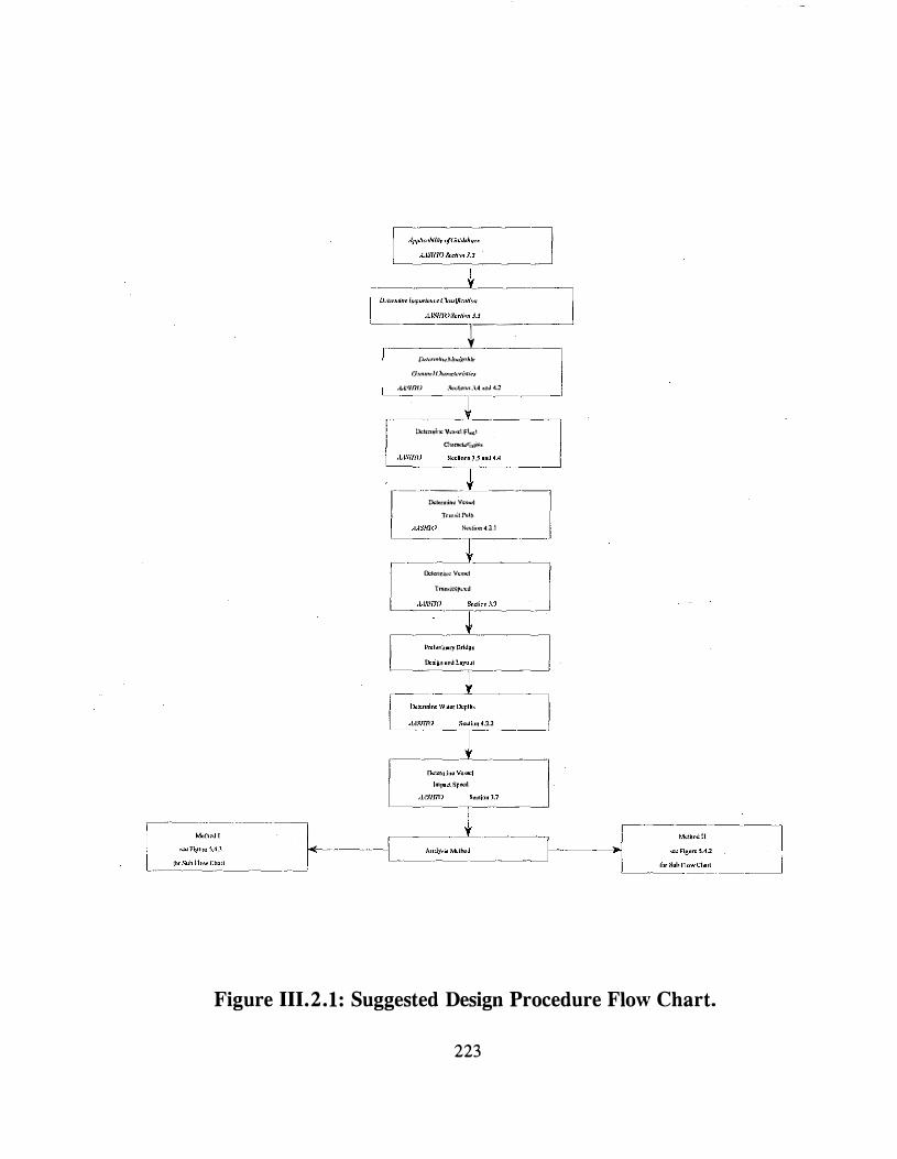
--] r ,= .... ,,-;::;:::,=:;::-- -� L .tl.�/nVI,!/omoJJ _j
-
-
]-
-_'!_ ---[ [k'""''""iln.,!<"hk J llwwro/1/,o�n•<l•.,.,.ll<r
,U\/ffl) .�<Ctinn.<.\4 onol 4.1 __ j__ =r -
.
. , .... ,,�::�:::.. 1 �ffl} �oollnn>l S onol 4 4 _ _j - - T - -1-- ___ 'j_ __ _ Dl:l•rmino v.� ... l
,.,. .. ,., �, �!n'O S«tinn 4.l.l
-
r-
-·
-
1 ____ '1_ J. DclortniH< Vc.""l
Tmn•itSp•'<d
L _ _''O"CSICm..'J r-·ti_"''-·'-·'---�--,,., .. ,,:"'''""' ···--
J Lllc.��non.!LnyuLLI
Figure 111.2.1: Suggested Design Procedure Flow Chart.
223

�-··-!
I othnd II nr AA�llTO luudc 1
·�·"111<-'U"n""dCo"'""""'"'l' Ji '" ' �·· '""''"" � ... "' 111&1>"·� llriU .. ,
M�/1'/'() �.ciLno4X · ·----..
lkt..�m;no """'tianco Cril<ri•
fo.rllrid�oC,.np<>ncn"
L_y _
'!!" fYt"' �''' oud
'� '"'"Y "ITrnvcl AA>IIfo) e t ' ' ' 1
--, · ���-·· y
_ ] J
....... ;.� .• ".. .. I A,L',Hf<L ',,., '""' < " ' ·'
-·- ··----···
I C_� �::=::: =-::::-
_ _] Figure IH.2.2: Suggested Sub Flow Chart for Method II.
224
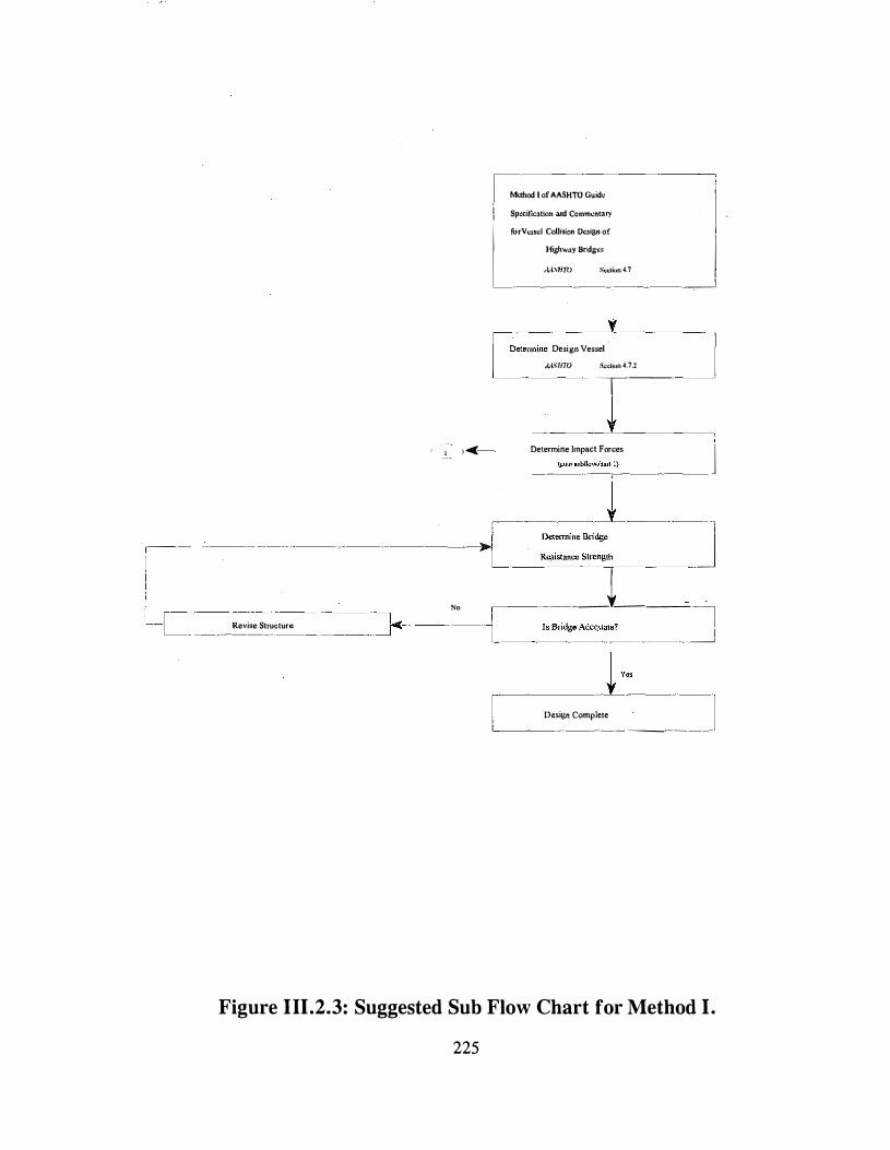
,------- - -
1
: _,- - �- � L_ Revise Structure ··------. ·
1�thod I of
-
AASHTO Guide �-i Specification and CommcnlaTY
L, f,o, ,y.,,., Collili"" ""''" of ___jll Highway Bridg�s
A:l.\1iTO Scclinn 4.7
_
-
-� J -
[:tennine Design Vessel
- -l "
,fASII1V Scoli"n 4.7.2 _ __j ' �-� •-<
-
Determine Impact Forces J -- '"'"""'"'"''""t--� ---···
�----
----� - :,:::::::::-----.- -J
No -[-.. ----�--� -·· --�goAdoqo:tr-
_!
_t:�-c - -- -� 1 Design Complete
� -- -- ----
----
Figure IH.2.3: Suggested Sub Flow Chart for Method I.
225
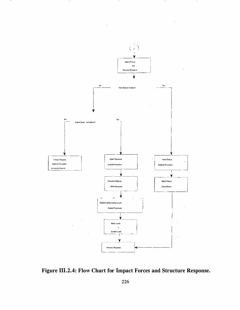
'" �-1 t
'" �- hli[\U�lSJ"CirumAuol)'<i<'l
l ,::�;:�';,:�:::: J ("'"''"'';"'""""'') ""-"---"
( I ) "_L C"""'""" �
""� \Un: !W>pmt""
-�y
�-""'"]];":: -.]. L:"ly•i•l'ro=lun:
--r -
[ -::;;,,,,_, -l Titn<!-�l"to"
··-··-� --�·1
Figure III.2.4: Flow Chart for Impact Forces and Structure Response.
226

III.3 IMPACT SPECTRUM ANALYSIS PROCEDURE (ISAP)
In the previous Section, the psuedo-dynamic analysis procedure (PDAP) was developed by utilizing the results of Section 4 where it was shown that the total modal response could be resolved into those modes for which the inertial effects are significant and those modes for which the inertial effects may be neglected. The impact spectrum analysis procedure (!SAP) will be developed using these same results; however, in this Section, it will be assumed that more than one inertial mode will contribute to the dynamic response of the structure. In addition, a discrete generalized modal formulation will be used for the inertial displacement rather than a continuous generalized inertial displacement as was used in the previous Section. Therefore, the mass of the columns will be lumped at the concentrated mass nodes. The column mass lumping will be discussed in more detail later in this section.
In order to develop the impact response equations Eqn. 4.32 is written for the maximum response over time as
d DMF
1 $ } " - l K 1< = rl - I
p l � l -· • [ k ] - I R }
K (Ill. I)
where the term, [k]''{R} is equal to the total static response of all modes (as discussd in Section 5). Therefore, Eqn. 111 .1 is written such that the total maximum response (f(t)=l.O), {vLax' is determined in part by modal analysis and in part by ordinary static analysis which is written
where
I " I mmlul
" { v } + { v l """'"' Hlulir
" DMF
E I � l " " I
I k I ' I R l
(111.2)
( ( . "' ) p d p . E I � l - (III.3a)
K n � I K
(III.3b)
Solution of Eqn. III.3a requires the determination of the multiple inertial mode shapes. The mode shapes will be derived on the basis that, in addition to
227
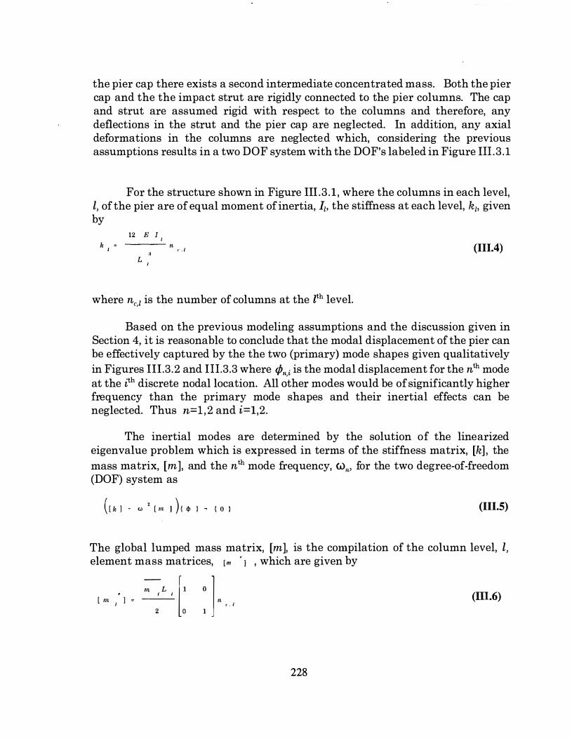
the pier cap there exists a second intermediate concentrated mass. Both the pier cap and the the impact strut are rigidly connected to the pier columns. The cap and strut are assumed rigid with respect to the columns and therefore, any deflections in the strut and the pier cap are neglected. In addition, any axial deformations in the columns are neglected which, considering the previous assumptions results in a two DOF system with the DOF's labeled in Figure Ill.3.1
For the structure shown in Figure III.3.1 , where the columns in each level, l, of the pier are of equal moment of inertia, I1, the stiffness at each level, k1, given by
k " 12 E 1 1
L
" <" . /
where n, 1 is the number of columns at the zth level.
(III.4)
Based on the previous modeling assumptions and the discussion given in Section 4, it is reasonable to conclude that the modal displacement of the pier can be effectively captured by the the two (primary) mode shapes given qualitatively in Figures III.3.2 and Ill.3.3 where ¢,. i is the modal displacement for the n1h mode at the i'h discrete nodal location. All �ther modes would be of significantly higher frequency than the primary mode shapes and their inertial effects can be neglected. Thus n=l,2 and i=l,2.
The inertial modes are determined by the solution of the linearized eigenvalue problem which is expressed in terms of the stiffness matrix, [k] , the mass matrix, [m], and the n1h mode frequency, U>,., for the two degree-of-freedom (DOF) system as
( [ k I - w ' [ m I ) t $ I l o I (111.5)
The global lumped mass matrix, [m], is the compilation of the column level, l, element mass matrices, 1m ' 1 , which are given by
[ m 1 ] �L , [ l O J "
2 0 1
(III.6) ' · '
228

where "' 1 is the mass per unit length of each column for level l, and the i <h DOF lumped nodal masses, m,. Therefore, using the modeling assumptions stated previously the global lumped mass matrix, [m], is given by
"' L "' L "' " " . "' " ' , . , 1 ,. ' 2
2 2
"' L
"' " . "' � . 2 ,. ' 2 2
"' "' 0 l ' 2 2 . 1
Writing
"' ' ' b .
"' . . , and m= m1 1 the global mass matrix is simply
[ /It 1 ["' 0 ) 0 b 1/t
(III.7a)
(III.7b)
(UI.7c)
(III.S)
(III.9)
The element stiffness matrix, [k'], is derived based on the rigid cross member assumption and the fixed base condition and is given by ,.
I k I I (111.10)
Using the two degree of freedom model assumptions and Eqn. III.5 the global stiffness matrix is given by
229

E I k -- n " ' (' . 1
L
E I ' k -- n � . 2 , . . 2 L k k - k I , 2 2 . I 2 . 2
Writing a •
and k E I L
' ' -- --
.� E I L '
E I '
L
E I ' -- .. ,. ' �
L
the global stiffness matrix is simply , [k • a k - a k I I k I • - a k a k Using Eqns. 111.9 and III.l4 Eqn. III.5 can be written [( l • a ) k - m }. - a k - a k 1 { <1> ) • { 0 ) a k - b m A
(HI.lla)
(III.llb)
(IU.llc)
(III.12)
(III.13)
(III.14)
(III. IS)
where A is the corresponding eigenvalue, w, which satisfies the non-trivial equality given by equation III.15. Solving Eqn. III .15 for mode n displacement vectors, <l>i ,, and frequencies, w,, where i is the node DOF number, and <Pi n is arbritrarily set equal to unity (scaled) for i = 1, gives the explicit m�dal displacements for i=2 and n=l, 2 which is expressed as
230
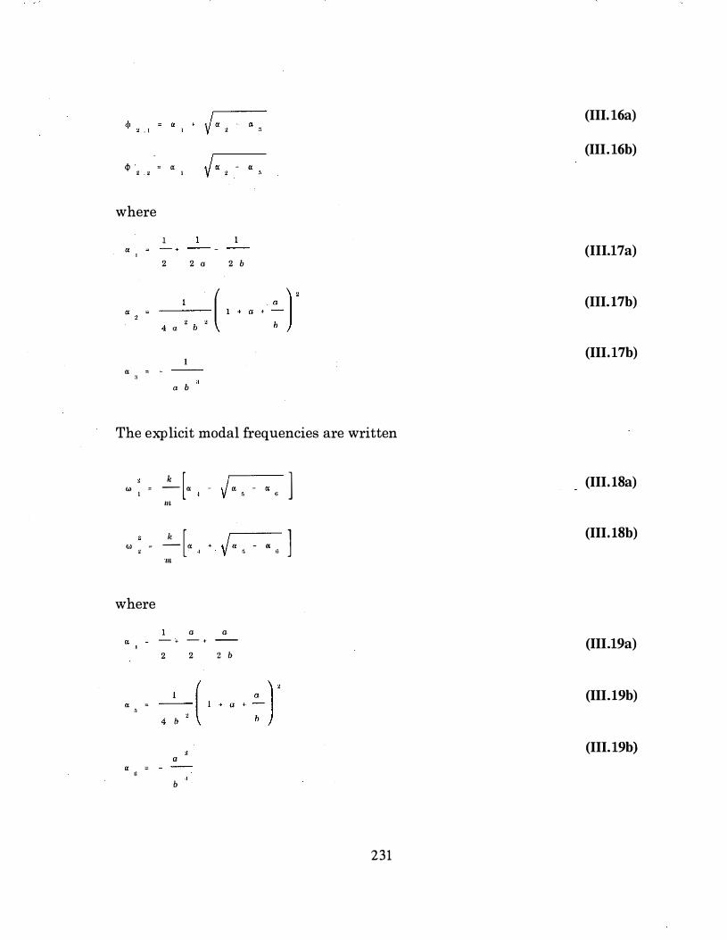
q, · "' a _ _ /rx - a 2 . 2 1 v 2
where
. " "
2 2 a 2 b
1
a b
The explicit modal frequencies are written
"' " '
"' " '
where
. " "
_k [. - J. -' " "'
_k [. ' . J. -'
"'
a a - + - + -
2 2 2 b
a
b
• ] • ]
231
(III.16a)
(III.16b)
(III.17a)
(III.l7b)
(III.17b)
(III.lSa)
(III.lSb)
(III.19a)
(III.l9b)
(III.19b)

The modal load, Pn, and modal stiffness, K,, were given previously in Section 4, but are repeated here, and are written
T p I <I> l I R } (III.20a)
K T
I 4> l [ k J I 4> l (III.20b)
where {R} is the peak barge impact load vector which is assumed, for the two DOF model, to be given by
{p "'" } I R } " 0
where Pmax is given by Eqn. 3.43.
(III.21)
Utilizing Eqns. III.l6 through III.21 the n'" mode lumped inertial forces, lfi.J produced by the individual modal displacement vectors, {u"}, (given by Eqn. III.3a) can be calculated from (e.g., Clough and Penzien, 1993)
{ {1 . 1, } = = - w [ m ] { u " ) (111.22)
However, the actual sign of the inertial vectors have little significance over the displacement time history; therefore, the maximum story shears will be given by the sum of the absolute values of the inertial vectors. In addition, the absolute value of the inertial force vectors are combined with the static response force vector, {R}, (refer to Eqn. III. I) to produce the total impact force vector, lfr} ,
II • ]
l i t l I • I R l / . "
Therefore, Eqn. III. l is written
d DMF ( w
I " l onn� I: l l <t> } " ' K 11 • I ' '
) p p I <I> } -· I · [ k J " ' I R }
" K : . '
to produce the maximum response and Eqn. III.23 becomes
232
(111.23)
(III.24)

U,. I (HI.25)
where d = 2. The actual member design forces and displacements are determined by utilizing fir} in a suitable frame analysis/design program. It is important to note that even though the inertial forces were calculated by assuming the simple two DOF model, the total impact design forces are applied to a suitably descretized model of the bridge pier. The following section will present the design procedure in a step-by-step format as was done for the PDAP in Section 5.
233
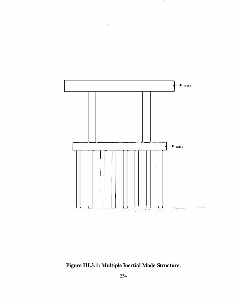
�-)-- DOF2
�.�-·--
�'-
- · ··-·
'--
-·
·
�·-'--'-··'--'- -c'_L _ _J+__Jc.J_--c- ··-�-· · · - - ··� .
. ·· .·
Figure 111.3.1 : Multiple Inertial Mode Structure.
234
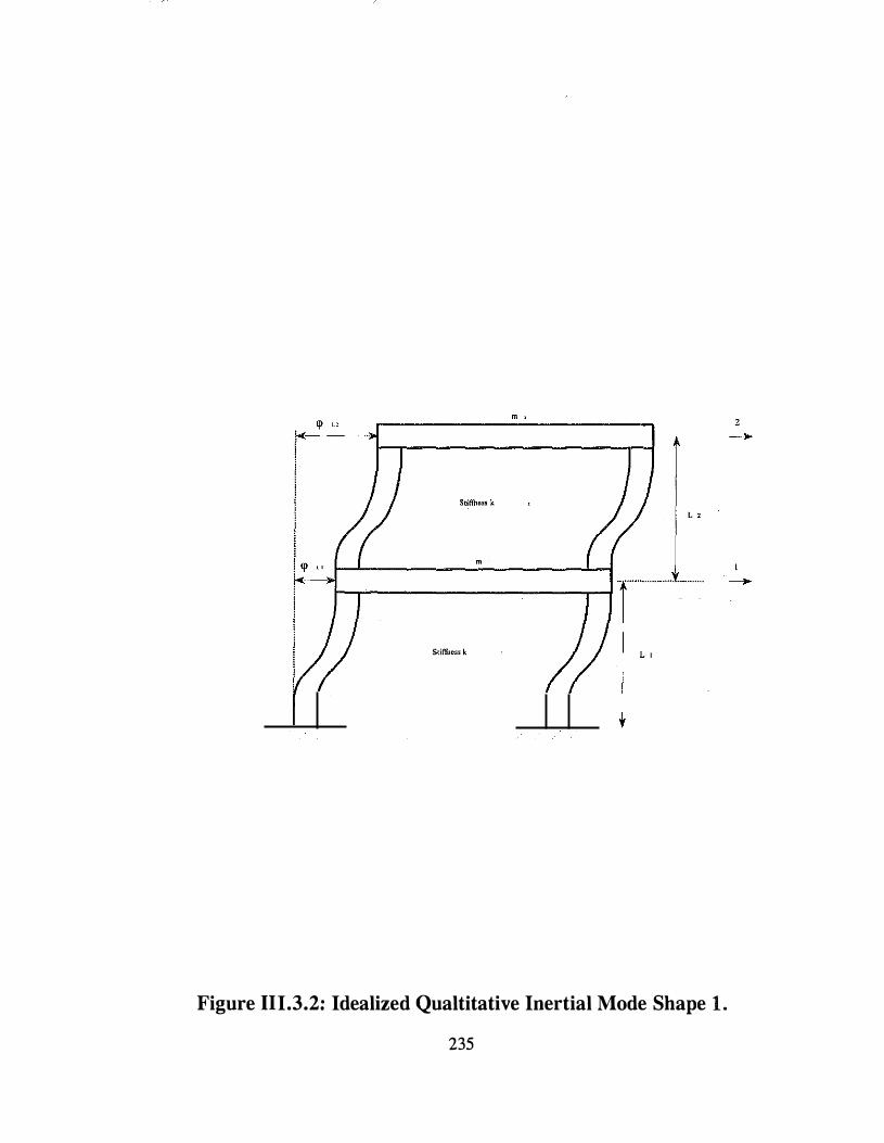
y
Figure UI.3.2: Idealized Qualtitative Inertial Mode Shape 1.
235

m '
L ' Stiffness k
� ; <p ' ' 1--r------------...--1 j
Stiffnuss k
L •
Figure IU.3.3: Idealized Qualitative Inertial Mode Shape 2.
236

III.4 STEP-BY-STEP ISAP
The methods given in this appendix have resulted in a simplified barge impact analysis procedure whereby the dynamic effects of the interaction of the individual barges in the flotilla and the bridge are included. The procedure to calculate the maximum impact displacement vector, {v(x)},.ax> and the resulting design forces using the ISAP are given in the following steps.
STEP 1 : The first mode displacement vector is given by
$ ' . " J" - " · ' '
� ' " J" - " ' '
and the second mode displacement vector is given by
$ ' . " J" -'
� ' . " J" -'
where
and
b .
E I L ' ' -- --
� E I L '
"' L "
2
"'
. . '
L
2
In addition
" "
"' L " • "' , . . 2
2
" • "' ,. ' 2
237
(III.26a)
(III.26b)
(III.27a)
(III.27b)
(III.28)
(III.29)

"
" � '
"
1 - , - _ _
2 2 a 2 b
1 c " a " �r 4 a 2 b 2 b
1
a b
STEP 3: The modal frequencies are calculated by
w � '
w � '
k [ .; l - a - a: - ct ·I r, G
"'
where
"'
and
k �
"' '
2
E I '
L
L
In addition
"' L ' ' n •. . l
2 n " "' , . . 2
238
(III.30a)
(III.30b)
(III.30b)
(III.31a)
(III.31b)
(111.32)
(111.7b)
(III.33)
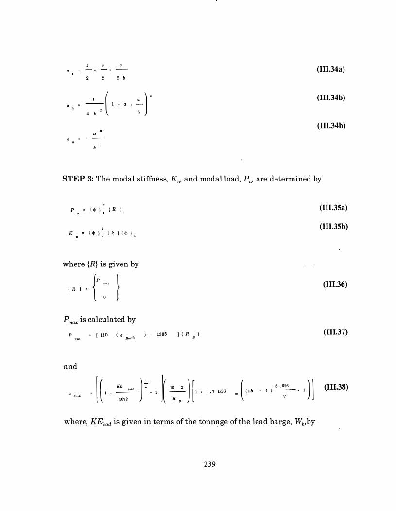
a "
" " '
a " ''
a a - . - . -
2 2 2 b
-� , C · a · �) ' 4 b b
a
b
(III.34a)
(III.34b)
(III.34b)
STEP 3: The modal stiffness, K., and modal load, P., are determined by
1' P " • I � } I R I .
1' K I � } I k l I � }
where {R} is given by
{p """ } I R } "
0
Pmax is calculated by
P "'"�
"' [ 110 ( a Rmuli ) + 1385 ] ( R JJ )
and
a Bmult
[ ( KE loot/ ) : ]( 1
0 2 ) [ ( 5 576 ) ] " 1
• 5672 - 1 -;-: 1 • 1 7 LOG '" ( nb - 1 )
V , 1
where, KEzead is given in terms of the tonnage of the lead barge, Wb,by
239
(111.35a)
(III.35b)
(III.36)
(III.37)
(III.38)

KE w v
32 . 2
STEP 4: The total impact design loading is calculated by
,,
E l w : [ m ' 11 " I I
'
( DMF
I I � I "
(III.39)
{ R I (III.40)
where d= 2, and the modal dynamic magnification factor, DMF((,Tp,,) (given here in terms of the structure undamped mode period, Tp,,) is determined for the multiple barge flotilla case from the following (assuming �= 5%)
DMF
DMF
and
T l' · "
( T ) o l o T p . n p . "
( T ) " I . 75 p . "
2 '
for
T s 0 . 75 p . "
T > 0 . 75 ' · "
For the single barge case the dynamic magnification factor is given by
[I kiF r r [ T p 11 l > o i . O o ll . l �
( T ) "' I . 4 + . . 'fl [ r , , - o " ]
r T = I "/:'") p . II •
f,_',,.
/r>r T
240
T
r
f' II s; (_) . JJ ::r'r:
0 . :::' ::e;
(III.4la)
(111.4lb)
(111.42)
(III.43a)
(III.43b)
(III.43c)

STEP 5: The member design displacements and forces resulting from the total impact design load vectors, ifr}, (calculated in step 4) are determined using a suitable space frame or finite element analysis/design computer program. It is important to note that the load vector, ifr}, is applied at this point of the analysis to the fully descretized pier model. Therefore, ifr} is non-zero only at the impact and lumped (concentrated) mass nodes. In addition, the load vector is the combination of the psuedo-static and two inertial modes response. As was exemplified in Section 5 for the PDAP, combinations of the psuedo-static and positive and negative direction inertial modes should be considered since the inertial mode loading reverses over the impact time history. Any one of the possible combinations may control the design of the individual pier members. For the two inertial mode case, there are four possible load combinations as will be shown in the following section in the form of a design example.
The calculations outlined in the preceding steps are easily completed using a computer spreadsheet program or similar software. Math Cad was used for the step-by-step calculations in the example problems given in the following sections along with GT-STRUDL for the fully discretized space frame analysis step (Step 5).
III.5 DESIGN EXAMPLE USING THE ISAP
A design example using the Impact Spectrum Analysis Procedure (ISAP) is given here, and the solution follows the step-by-step procedure presented in the previous sections. The bridge pier is to be designed for impact by a flotilla column of four 35'x195' barges traveling at an impact velocity of 17 fps. Each barge has a combined dead weight and cargo tonnage of 3800 kips. The example pier (shown in Figure III.5.1) is comprised of 48 piles (8x6 pile group shown in Figure III.5.2, 1=3200 in4for each pile) that are rigidly connected to the pile cap. In addition, the piles are assumed fixed at the the ground elevation. Two pier columns of 1=260,000 in4 (each) support the pier cap. The nodal mases and stiffnesses were determined using Eqns. III.26 and III.27, respectively.
The idealized pier dynamic model used to determine the impact loads is shown in Figure III.5.3. The calculated pseudo-static, inertial mode 1, and inertial mode 2 loads are shown in Figures III.5.4. Only the relative direction of the loads for each mode is important. Examination of the results given in Figure III.5.4 reveals for this design example the second inertial mode (Figure III.5.4b) contributes little to the overall structure response as is indicated by the fact that the second mode total inertial shear is only 4.75% of the psuedo-static component (Figure III.5.4a). The actual signs of each component of the impact loading (pseudo-static, mode 1, and mode 2 components) are applied in all direction
241
combinations to possibly produce worst case loadings for each member (i.e. design load combinations). The four possible direction loading combinations are shown as Figures III.4.5a through III.4.5d.
The pier response due to the load combinations given in Figure III.5.5 were determined using the GT-STRUDL finite element computer program and a fully descretized pier model. The piles and columns were subdivided into four beam/column elements and the pier cap was descretized into three elements. The pile cap was modeled using four-node quadralateral and three node triangular plane-stress/plate bending (six DOF/node non-coplanar) overlay finite elements. The finite element mesh is shown in Figure III.5.6.
The responses determined using both !SAP and the current AASHTO equivalent static method are compared to the response determined using a linear time-history analysis (direct time integration) from the load time history determined in Section 3. All analysis results given in this section were calculated using the GT -STRUDL computer program. These results are given in Table III.5.1 where it can be seen that the maximum response determined using the time history is within 4% of the response determined using the !SAP method. However, the equivalent static method varies by over 34% from the time-history method.
As was pointed out in the previous Section, the equivalent static method will usually be significantly different from the design loads determined using any of the recommended design procedures. This is due in part to the fact that the AASHTO method neglects the loading that results from the inertial effects. In addition, the peak impact load determined using the equivalent static method does not take into account the dynamic interaction of the individual barges in the flotilla and the dynamic interaction of the barges and the bridge pier.
242

I ! !
Node 2
35ft.
42ft.
�----- ------- --�: 55 ft ---------- J --------,---,-�, " -----r-�
�-:�· (<yp.) -l�i ' " 25ft.
4-+---- ------- " -
I= 443,000 in.
Node I
1=1 ,080,000 in
s ft.
1=4000 in.
I _!__ _ - -- l _ I _ -�-_L__- ----- __jj"C" _ c����-----�L_ ______ _
Drawing not to scale
Figure HI.S. l : Design Example Pier.
243
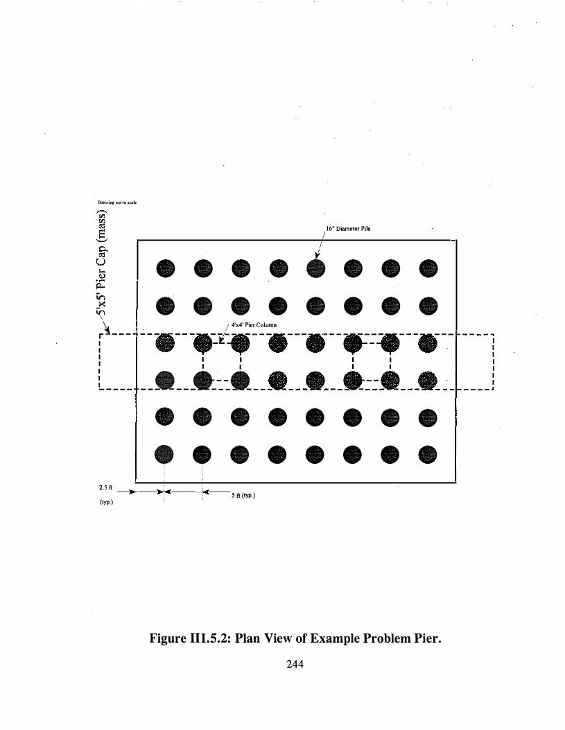
Drnwing not to scale
16" Diameter Pile I
I • • • • ' • • •
� • • • • • • • • '\'\ /_ 4'x4' Pier Column fL _ _
- -.- - -.,.:�lJ - - .- - -. - -.,::llt- - -.- - r - - - - 1 : I I I I 1
L _ _ _ _ --�---41t::tlt _ _ �---�---�::�---�-�-r-- - - j • • • • • • • • • • • • • • • •
2.5 ft -'J>c--·--l< (typ.)
5 ft (typ.)
Figure HI.5.2: Plan View of Example Problem Pier.
244

L , 12
p ••
Node 1 Tribut;ny Mass An:"
Node 2
·---�----------,----,-/ Node I
,; ' -- -- - ------- ----- _ _j I
Noll<: 2 Tributm)' Mass Area �
- - - A
Figure IH.5.3: Idealized Example Problem Pier.
245

3077 kips- I
I L_ ��_J_l_ __
(A)
7.78 kip/ft �-�- _,. _.,. -). __ ,. •
--�- --
1 I 1 � .40 �p/ft •
L r !
(B)
. I
1.0 kip/ft ..,. __ _. ...:- � ..(--- ..,;•
1.69 kip/ft _,. ... .. =>··•.L.L.., L .1
�--=--
I ' / _/ ,--;�---_1.--
(C)
Figure IU.5.4: Calculated Loads, (A) Psuedo-Static, (B) Inertial Mode 1, and (C) Inertial Mode 2.
246
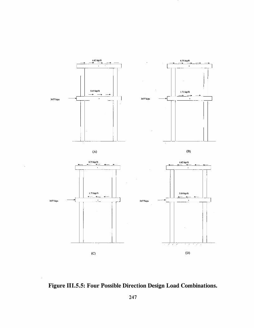
3U77 kips
3[)77 kips
6,82 kiplfl
- - ...
5.!19 kiplfl
(A)
8.75 kip/fl c -=--=--·- -_" = -�::J
1.71 kiplfl
---�--== ' : _" -�- ]
(C)
3U77 kips
3077kips
lJl kipln
'-,-,--�-'-· " --,-_j
- -·C
(B)
6.H2 kiplfl t:-� .. �
5.09 kiplfl
(D)
- -:!;:;==
Figure HI.5.5: Four Possible Direction Design Load Combinations.
247

Drawing not to scale
3-Node Tn (6 DOF/no
· � ang e de)
,./'
/ v
1 4-Node Quadralateral (6 DOF/node)
"'-../ i"'-.. / I :/"'-.. 1/"'-..
.
I/2-No Fram
de Space
e Element
(6 D OF/node)
Figure III.5.6: Example Problem Finite Element Model.
248
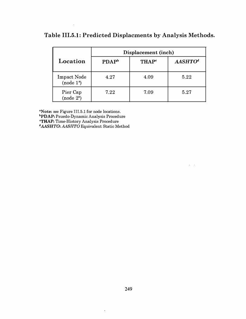
Table III.5.1 : Predicted Displacments by Analysis Methods.
Displacement (inch)
Location PDAPb
Impact Node 4.27 (node 1 ")
Pier Cap 7.22 (node 2")
•Note: see Figure III.5.1 for node locations. hPDAP: Psuedo-Dynamic Analysis Procedure 'THAP: Time-History Analysis Procedure dAASHTO: AASHTO Equivalent Static Method
249
THAPC
4.09
7.09
AASHTOd
5.22
5.27

III.6 CONCLUSIONS
The methods presented in this Section are intended to improve the analysis of bridges susceptible to barge flotilla traffic. It was shown that there is a considerable difference between the response calculated using the current AASHTO equivalent static method and the Psuedo-Dynamic Analysis Procedure given in this Section. The current AASHTO analysis procedure does not include the effect of the interaction between the individual barges in the flotilla and the bridge pier. This is significant since the energy lost between the individual barges in the flotilla column was found to be very significant using the analysis techniques given in this Section.
Another important difference between the two methods is that the current AASHTO analysis procedure neglects the member loading that results due to the inertial effects of the impact loading time history, whereas the inertial loading is included with the Psuedo-Dynamic Procedure. Depending on the structure dynamic characteristics, the inertial member loads could increase the member design loads by up to 70% as compared to the equivalent static procedure loads.
It was shown in Section 4 that the total modal response could be resolved into those modes for which the inertial effects are significant and those modes for which the inertial effects may be neglected. The structural response for which the inertial effects may be neglected is called the psuedo-static responsJ').
250