Embed Size (px)
Citation preview

ANALYSIS AND DESIGN OF BEAM-COLUMNS
by
CHENG-HSIUNG CHEN
Diploma, Taipei Institute of Technology, 1959
A MASTER' S REPORT
submitted in partial fulfillment of the
requirements for the degree
MASTER OF SCIENCE
Department of Civil Engineering
KANSAS STATE UNIVERSITYManhattan, Kansas
1967
Approved by
Major Professor

TABLE OF CONTENTS
SYNOPSIS 1
INTRODUCTION 1
METHODS OF ANALYSES 4
General Method 4
Energy Method 13
Numerical Method 19
Moment Distribution 29
DESIGN METHODS 38
Secant Formula Method . 38
Interaction Formula Method 44
Example 48
CONCLUSION . ....... 52
ACKNOWLEDGMENT 54
NOTATION 55
BIBLIOGRAPHY 57

SYNOPSIS
An "exact" method and three approximate methods for the analysis of the
behavior of members subjected to bending moments and axial compression are
reviewed on the basis of elastic theory. Sample problems that are frequently
encountered in steel structures are treated. The effects of lateral and
torsional buckling are not included. Two design methods that are adopted in
the AISC (14) and AASHO (15) Specifications are described and a design
example is worked in order to illustrate the design procedure according to
the AISC Specifications (14).
INTRODUCTION
This paper contains a review of analysis and design procedures for
steel members subjected to combined bending and compression. The bending
may arise from transverse forces and/or from known eccentricities of the
axial loads at one or both ends. These kinds of members are generally
referred to as beam-columns. Beam-columns are commonly analyzed and
designed as isolated members, whereas in practice they are usually parts
of a frame. In framed steel structures, there are three categories of
individual members:
(1) Beams. Beams are members subjected to forces which predominantly
produce bending.
(2) Columns. Columns are members axially loaded predominantly in
compression.
(3) Beam-columns. Beam-columns are members whose loads are a combina-
tion of the loads on beams and columns as stated above.
When the bending is small compared with the axial force, the bending

can often be neglected and the member can be treated as a centrally loaded
column. On the other hand, when the axial force is small compared with the
bending, the axial force may be negligible and the problem becomes that of
beam analysis.
The basic equation for analyzing a beam-column problem is based on the
relationship between the moment and the curvature of a beam, i.e., Ely" = -M,
and takes into account the compressive forces. In the equation Ely" = -M,
E, I, y" , and M are modulus of elasticity, moment of inertia, curvature, and
moment, respectively. Professor N. M. Newmark (1) has developed a numeri-
cal approach which provides a means for obtaining an approximate but satis-
factory solution for beam-columns. The energy approach is also an approxi-
mate solution, but it is a convenient method when the loadings are
complicated
.
Early solution of beam-column problems have been reviewed by Bleich
(2). Ketter, Kaminsky, and Beedle (3) have presented a method for determin-
ing the plastic behavior of laterally supported wide-flange shapes under
combined axial forces and moments. Galambos (4) and Ketter (5) have
presented numerically determined interaction curves for the maximum strength
of beam-columns under various end conditions, including the effect of resid-
ual stress. The effect of end restraint on the eccentrically loaded column
has been explored by Bijaard, Winter, Fisher and iMason (6). Two approximate
methods for estimating the strength of beam-columns have been reviewed by B.
G. Johnston (7), the first method is based on the concept that the load
which produces the initiation of yielding in the fiber subjected to the
Numbers in parentheses refer to the numbered references in the biblio-graphy.

maximum stress provides a lower bound of the failure load, and the second
method is based upon the interaction equations.

METHODS OF ANALYSES
The purpose of the following analyses is to show the procedures for
finding the maximum deflection and maximum bending moment of a member sub-
jected to moment and axial compression simultaneously. The general method
is an "exact" method, while the numerical method and the energy method are
approximate methods.
GENERAL METHOD
By neglecting the effects of shearing deformations and axial shortening
of the beam the differential equation (8) of the axis of the beam-column as
shown in Fig. 1 can be expressed in the following alternate forms
Ely" = - M ,
Ely" 1 + Py' = - V ,
Ely ,v/ + Py" = q .
(1)
(2)
(3)
The differential equations can be solved by use of the given boundary condi-
tions, and consequently the deflections, bending moments, and end rotations
may be obtained. Three examples of the use of this method are given in the
following sections.
The bending moments and forces shown in Fig. 1 are assumed to be posi-
tive in the directions shown unless otherwise noted.
p A rj-nn /-q
M I J I I 1
b P
3*P^dx
X x P
m
MA 'i
r-iCJTO]
Q in
M+dM
dx
V+dV
Fig. 1. Sign conventions
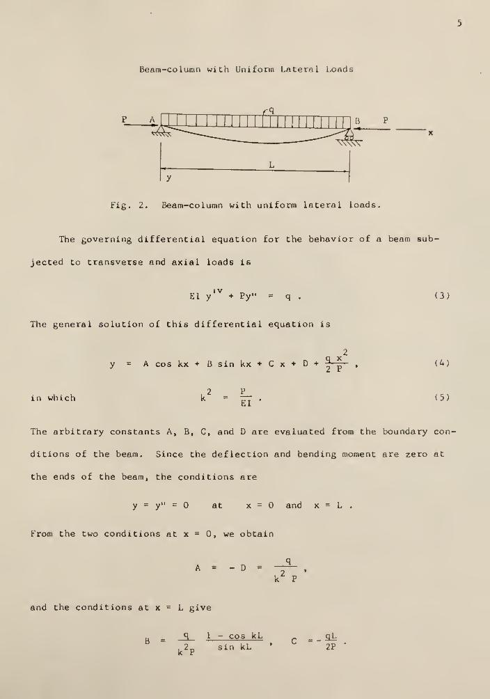
Beam-column with Uniform Lateral Loads
Fig. 2. Beam-column with uniform lateral loads.
The governing differential equation for the behavior of a beam sub-
jected to transverse and axial loads is
IVEl y + Py" = q .
The general solution of this differential equation is
2Q x
y = A cos kx + B sin kx + C x + D + *,
, 2 P
(3)
in whichEI
*
(4)
(5)
The arbitrary constants A, B, C, and D are evaluated from the boundary con-
ditions of the beam. Since the deflection and bending moment are zero at
the ends of the beam, the conditions are
y = y" = at x = and x = L .
From the two conditions at x = 0, we obtain
A = - D =2
k P
and the conditions at x = L give
q 1 - cos kLy _ 1_
, 2__ sin kLk P
-_SJL2P

Substituting these values of the constants into Eq . 4, the equation for the
deflection curve is found to be
y=
Elk4
sin kx + sin k(L-x)sin kL
- 1
2EIk'
x ( L-x
)
(6)
Letting x=L/2 in Eq. 6, the deflection at the center-line of the beam is
found to be
A = (y) J^k f,(u) ,
where
and fx(u)
x=L/2 384 EI 1
u - kL/2 ,
12(2 sec u - 2 - u2
)
5u4
(7)
(8)
(9)
By taking the first derivative of Eq. 6, we obtain an equation for the slope
at any point on the beam. Letting x=0 yields
3
9 = 9,a b (y')_n ?7T7 f o<">
where f2(u) =
x=0 24E1 2
3 (tan u - u)
3u
(10)
(11)
The bending moment at the center of the beam is given by
2
M = " E1( *M)x=L/2
qL
where f3(u)
8
2(1 - cos u)
f,(u) , (12)
(13)
u cos u
The first factors on the right-hand sides of Eqs. 7, 10, and 12 are the
values produced by a uniform load acting alone, and the second factors
f.(u), f„(u), and f»(u) represent the effects of the axial compression
forces.
Tables of these functions have been provided in the Appendix of
Reference 8.

Beam-column with a Concentrated Lateral Load
Fig. 3. Beam-column with a concentrated load.
The bending moments in the left- and right-hand portions of the beam in
Fig. 3 are, respectively,
ML
= 9£ x Py, M . q a - sJ (L_X) + Py §
R L
Using Eq. 1, we have
Ely" = - . x - Py , and
Eiy- Qih - c)(L - x) - Py
The general solutions of these equations are
Qcy = A cos kx + B sin kx - rr x , and (14)
y = C cos kx + D sin kx - Q (L-c)(L-x)PL
(15)
By use of the end conditions y = at x = and at x = L, we obtain
A =, C = - D tan kL .
Similarly, using the fact that the slopes and deflections of each segment
must be equal at the point of application of the load Q, i.e. y y andL K
y' = y' at x = L - c, we obtainL K

Q sin kc Q sin k ( L-c
)
Pk sin kL ' Pk tan kL" *
Substituting these values of the constants into Eqs. 14 and 15, we obtain
the following equations for the two portions of the deflection curve:
_ Q sin kc . . Qc n ^ ^ . ,,,.*L Pk sin kL
^"kx-^x, 0<x<L-c (16)
yR' SM^ - «^, - «U-iU-l . L-c_< X <L «»„
By taking the first and second derivatives of Eqs. 16 and 17, the expres-
sions (8) for slope and curvature can be obtained. In the particular case
of a load applied at the center of the beam, the maximum deflection, end
rotation, and the maximum bending moment are obtained by substituting c=L/2
and the appropriate values of x into Eq. 16. This procedure gives
A =(3"x.l/2
= Sn •£2
(u)•
(I8)
2
9 = 9, = (y«) _ = f^TT • f, (u) , (19)a b ' x=0 16E1 3
M = - EKy") ,., = * ^"^. (20)
r x=l,/2 4 u
Again, the second factors on the right-hand sides of Eqs. 18 to 20, f (u),
f_(u), and (tan u)/u are the effects of the axial compression on the beam.

Beam-column with Couples
M,
r^&K *b
P f * -) \—:a^~If B^P-Z*^fer
-LiA B
(a) (b)
Fig. 4. Beam-column with couples.
If two couples M and M, are applied at the ends A and B respectively,
the bending moment at any section in the beam is
M - M.
M = M - -~ X + Py .
a L J (21a)
Using Eq. 1, we obtain
M - MEly" = - M + -*-: — x - Py
a Li
The general solution of this differential equation is
M - Mu M. , n • i a b a
y - A cos kx + B sin kx + — x -
EIk2L Elk
(21b)
By using the condition y = at x = and x = L, we obtain
A =Ma
P 'B = r— — (M, - M cos kL)
Psin kL b a
By substituting these values of A and B into Eq. 21b, we obtain
sin k(L-x) L-xsin kL L
M,sin kxsin k L
x
L(22)
The bending moments M and M, may arise from eccentrically applied

10
compressive forces P acting as shown in Fig. 4b. By substituting M = P e
and ML= P e L in Eq . 22, we obtain
b b
,sin k( L-x) L-x s sin kx x,
y = e ( ;
—
~— - —— ) + e, (~
—
— - r) .
a sin kL L b sin kL L(23)
The end rotations 9 and 9 in Fig. 4a are obtained by taking the first
derivative of Eq. 22 and letting x=0 and x=L, respectively. The rotations
may be expressed as
M L ML9a
=(y>x=0
=3E1
f4(u) +
biT£5(U)
•(24)
M L ML-
( y ,}x=L
=6il
£5(u) +
3il£4(U)
'(25)
where f i s 1- A __1__.f , (u) = — (— - 7 — ) ,4 2u 2u tan 2u
(26)
f c (u) = - (—:
— - —5 u sin 2u 2u
) . (27)
Again, the factors f/(u) and f,-(u) in Eqs. 26 and 27 are the results of the
effects of the axial compressive forces on the beam. In the case of two
equal couples M = M = M , we obtain from Eq. 22
y = ML 2
8EI 2u cos u
. 2ux,cos(u - ~— ) - COS u
la
(28)
The deflection at the center of the beam is obtained by substituting
x=L/2 in Eq. 28; this gives
A =( ^x=L/2
ML t c *
8EI£3(U) (29)
Tables of these functions have been furnished in the Appendix of
Reference 8.
11
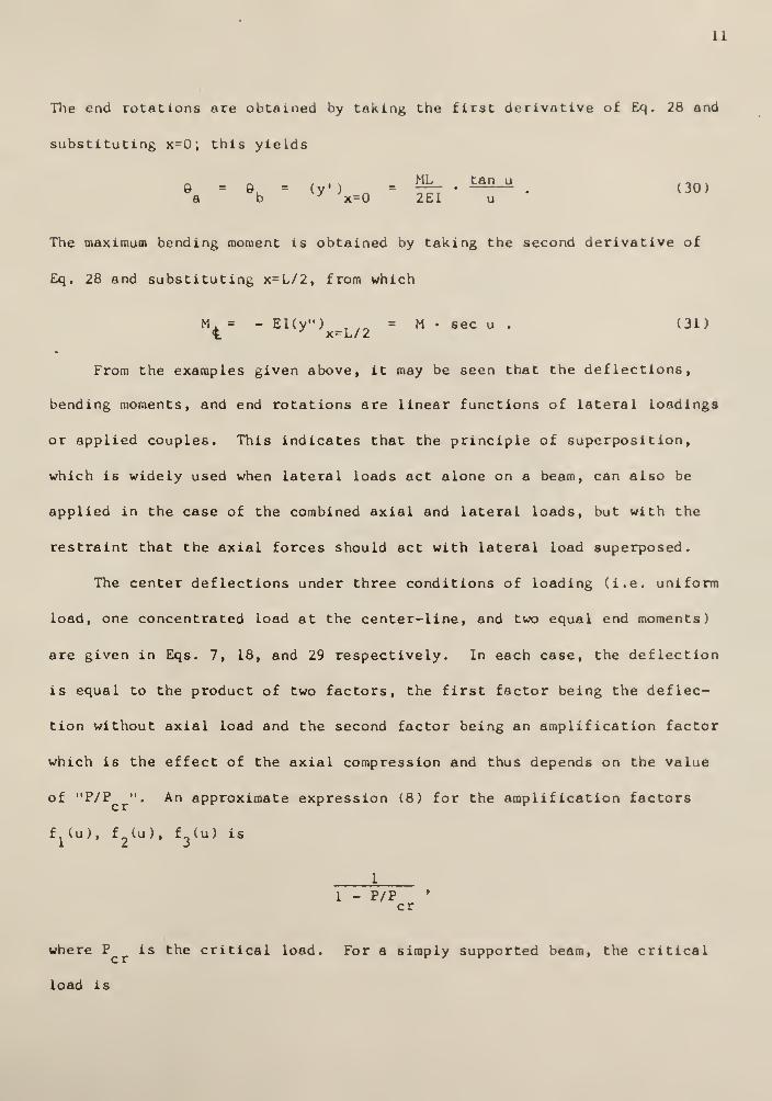
The end rotations are obtained by taking the first derivative of Eq . 28 and
substituting x=0; this yields
6 = *h = <y'>n = TFT '
^^ ' (30)a b x=0 2E1 u
The maximum bending moment is obtained by taking the second derivative of
Eq. 28 and substituting x=L/2, from which
M . = - EKy") f .„ = M • sec u . (31)£ x=L/2
From the examples given above, it may be seen that the deflections,
bending moments, and end rotations are linear functions of lateral loadings
or applied couples. This indicates that the principle of superposition,
which is widely used when lateral loads act alone on a beam, can also be
applied in the case of the combined axial and lateral loads, but with the
restraint that the axial forces should act with lateral load superposed.
The center deflections under three conditions of loading (i.e. uniform
load, one concentrated load at the center-line, and two equal end moments)
are given in Eqs. 7, 18, and 29 respectively. In each case, the deflection
is equal to the product of two factors, the first factor being the deflec-
tion without axial load and the second factor being an amplification factor
which is the effect of the axial compression and thus depends on the value
of "P/P ". An approximate expression (8) for the amplification factors
f.(u), f (u), f (u) is
1 - P/Pcr
where P is the critical load. For a simply supported beam, the critical
load is

12
2TT EI
cr
This approximate expression for the amplification factor can be used with
good accuracy, in place of f (u), f (u), and f„(u). For values of P/P
less than 0.6, the error is less than 2 per cent (8).

13
ENERGY METHOD
The energy method is widely used in structural mechanics; it represents
a unique mathematical application of the basic law of conservation of
energy. In applying this method to beam-column problems, it is necessary
to assume a deflection curve for the beam-column which satisfies the end
conditions of the beam. A deflection curve often used is expressed by
y = Z a sin — , (32)n L
n
where the a are the undetermined maximum amplitudes of the corresponding
sine curves. Assuming a virtual deflection da of the beam, the strainn
energy of the beam will increase an amount equal to AU while the external
loads do work equal to AT. Letting
AU = AT , (33)
where U = ^—7* = f1 (y")
2dx
,(34)
2EI 2
the coefficient a can be determined, and consequently the deflections, end
rotations, and bending moments can be found. The three examples given
before are treated by this method in the following sections.

Beam-column with Uniform Lateral Loads
14
P A
dc
1 I I 1 1 1 1 II KSI I I I I I fI I II I 1 D B P
Fig. 5. Beam-column with uniform lateral loads
Using Eq. 32, the strain energy of bending of a beam is
u = II !
'
(„)2 dx
2t
ei r
2I
l r- 2
l. n
2 2n tt n tt x
12
nL2
sin dx ,
orEITT 4 2
U = r— 2 n a/T 3 n4L n
(35)
The strain energy increase due to the virtual change da in a is
AU = 4^ daEITT 4
= r— * n a daBa n „.3 n n
n 2L
(36)
The horizontal displacement (9) of end B, which is equal to the difference
between the length of the deflection curve and the length of the initial
straight form, is
i r 2s = -
:(y' ) dx
2b
77- 2 a n4L n
n
(37)
The change in s due to the virtual change of da in a is& & n n

15
2
ds = -r da = —7 * n a da . (38)da n 2L n n
Work done by the axial force P is
AT, = P • ds = ^7- • n2
a da . (39)1 2L n n
Work done by the uniform lateral load is
AT„ = (q dcHAy) = ^r - da , for odd values of n. (40)2 v x=c 11 n n
Substituting the values of AU and AT (sum of AT and AT ) in Eq. 33 gives
4
a = —7— "T
—
Z , for odd values of n, (41)n
TT EI n (n - °L )
where ok = P/Pcr
Substituting this value of a into Eq. 32, yields the equation for deflec-
tion curve.
44qL _ 1 n -tt x , , _
,
y = —t— i* -3
—
-Z sin —— . (42)
TT EI n=odd n (n - o< )
Using only the first term of Eq . 42, the deflection at the center of a beam
is
A (v)^ql
41 = 5.03 qL
A1 .,-.
^ y x=L/2 J ri (1 - « ) 384 EI (1 - o< )
*
TT EI
The bending moment at the center of the member is
M = SL2- , pZ = flk! + 3.03 qL
AP
8 ^ 8 384 EI (1 - U )'

Beam-column with a Concentrated Load
16
Fig. 6. Beam-column with a concentrated load.
Assuming that the deflection curve is as expressed in Eq. 32, the
change in strain energy of the beam due to the change da in a isn n
AU =EITT
2L3
n a dan n
(36)
Work done by the external forces P and Q due to the change da in a is° n n
given by the following equation:
AT = P • ds + Q • (Ay)x=c
Pit 2 n it c ,——— n a da + Q • sin —r— da2L n n L n
By use of the fact that AU = AT, we obtain
13
20L*n tt-^t 2,2
TT El n (n - o( )
Substituting this value into Eq. 32 we obtain
3
sinn ttc
(45)
12QL~
4 * 2 2TT El n n (n - (X )
ntr c . nir xsin ~ sin ~*j
Li A-j
(46)
The center deflection and center moment respectively are given by the follow-
ing expressions:
om Jl QftA or
J
(47)2QL
31 .986 QL
31
y x=L/2 _4_. 1 - o< 48 EI 1 - X »
TT EI
M = 2L =QL .986 QL P
M4 * ™ 4 48 EI (1 - cX ) '
(48)

17
Beam-column with Couples
A * aMi
B >l_
P . A ^ a
(a)
B _ P P A
y (b) y (c)
Fig. 7. Beam-column with couples.
In order to simplify the problem, we may divide the problem of Fig. 7a
into two problems as shown in Fig. 7b and 7c by applying the principle of
superposition. In solving the problem of Fig. 7b, we use Eq. 32 as the
assumed deflection curve; then the change in strain energy due to the
virtual change dain a is the same as that given in Eq. 36. Work done by
the axial force P and the applied couple M due to the virtual change da
in a is expressed asn r
AT = P • ds M • d© .
a a
The term ds has been given in Eq. 38 and d9 is the angular displacement due
to the virtual change da in a ; this may be expressed as
de"* a
dax=0
nTT .
L n(49)
from which the following equation is obtained

18
M n-rr 2 2
AT = -~ da + " """• a da . (50)
L n 2L n n
Setting AU = AT, we obtain
2M L2
an
= -^ f . (51)TTJEI n (n - o( )
Using this value in Eq. 32, the following result is obtained
2M L2
a v 1 nTT x ._..y = r £ sin —— . (52)
TTJEI n n (n - « )
The deflection curve of the beam in Fig. 6c is obtained by using (L-x)
instead of x and M, instead of M in Eq. 54, which gives
b v 1 , n IT ( L-x
)
/c ~.y = —z— Z sin : fc
. (53)TT
JEI n n (n - <X )
By applying the principle of superposition, the deflection curve of the beam
in Fig. 6a is found to be
2M L2
,2M, L
2, „ .
a „ 1 nnx b v 1 nTT (L-x) ,_. .
y = - I sin — + —-— I sin r . (54)
TT EI n n(n - cX) TT^EI n n(n - o<
)
For the case of two equal moments M = ML = M , the deflection curve is
4M L2
Q „ 1 .nTT X ,rcw
y = —-— 2 sin — . (55)TTJEI n=odd n (n - o< )
Since the series is a rapidly converging one we can obtain reasonable
approximations to the center deflection and center moment by taking the
first terra of the series, as indicated in the following equations
4 M L2
, 1.03 M L2
. _ / v o 1 o_ 1 , a >
X=L/2=
"rT1^ 1
"1^ =
8ei r^^ •(56)
1.03 ML2
M = M+P-A = M+ QC. T
°"J
~. (57)
o o 8E1 1 - ctf

19
NUMERICAL METHOD
By applying the conjugate-beam method, Newmark (1) has developed a
numerical procedure for the determination of deflections and moments of a
beam-column with lateral load. This procedure eliminates much of the
mathematics of the "exact" differential equation approach or the finite
difference approximations. When the bar has a cross section which varies
along the span or has a complicated distributed loading, a numerical proce-
dure of successive approximations is quite useful. The purpose of this
section is to compute the deflections and the moments of a beam-column by
use of Newmark' s numerical procedure.
The relationship between the distributed load q, shear force V, moment
M, slope 9, and deflection y of beams are well known. They can be expressed
as follows:
dvq dx
VdMdx
m_ 19El dx
9dy_
dx
or = jqdx ,
(58)
ror M =
i vdx,
9 =J EI
dx'
or y = 9dx .
From the above equations, the shears, moments, slopes and deflections
of a beam can be determined by successive numerical integration.
In using this method, a beam is divided into segments and the distrib-
uted loading is reduced to equivalent concentrated loads at each division
point, or station along the beam. The equivalent concentrated loads at
stations are equal and opposite to the reactions at the stations when the

20
segments of the beam between the stations are treated as simply supported
beams. The variation of the distributed load (10) can be assumed to be:
(1) Linear between stations (Fig. 8a, b)
,
(2) A second-degree Parabola (Fig. 8c, d).
An example is given in Table 1 to illustrate the application of New-
mark's numerical method. The steps for computing deflections and moments in
a beam-column are as follows:
1. Compute deflections and moments due to lateral loads alone:
a. Obtain the values of moment at each station.
b. Compute the M/EI values which are the fictitious loadings in the
conjugate beam.
c. Compute equivalent concentrated loads "R" at each division point
by using Fig. 8c and d.
d. Calculate "Average Slopes" which are the fictitious shearing forces
in the conjugate beam. Due to symmetry, the reaction at the left
support is equal to one-half of the equivalent concentrated load
"R", i.e.,
(6.84 + 8.54 + 7.42) +J
(7.92) = 26.76 .
e. Compute deflections, "y ", which are the fictitious moments in the
conjugate beam due to the lateral loads alone and are obtained by
the following equation:
where
M. = M. . + V, • d ,
d = segment length,
V = Fictitious shearing forces in conjugate beam
between station "j" and "j-l", and

nra mn
nra7 (2a+b)o
R = 7 (a+Ab+c)n 6
mn 7 (2b+a)o
(a) (b)
nm ran
nra
mn
24
d
(7a+6b-c)
24
(c)
(3a+10b-c)
R = 7- Ca+lOb+c)n 12
Id)
Fig. 8. Equivalent concentrated load.
21
b
n
d d
"1 U\
d d

22
j = Station number.
Calculation of buckling load:
a. The procedure is to estimate a reasonable trial deflected configura-
tion and calculate the trial bending moments produced by the axial
load. Due to symmetry, the values of y, selected in Table 1 arelc
ordinates to a sine curve. The deflections produced by these bend-
ing moments are then computed (same procedures as stated in Step 1
above) and compared with the estimated trial deflections. The
ratios of the assumed deflections y to the computed deflections
y must equal one for the stable configuration to exist (11).
Considering the maximum and minimum values of the ratios, we see
that the upper and lower limits for P arer cr
15.35 EI j s 17 EI
L2
< « L2
•
b. The results can be improved by repeating the cycle of calculations.
The second cycle begins with the deflections y , which are propor-
tional to the deflections y found from the first cycle of computa-
tions. These values can be multiplied by any constant factor in
order to adjust the order of magnitude of the figures. In this
case, they are multiplied by 100/376 in order to give a as the
deflection at the center. The results of the second cycle show that
the load P is between the valuescr
16.4 EI ^ / 16.7 EI
L2
< Cr<L2
'
To obtain a more accurate result, we can calculate average values
(8) of the deflections y„ and y_ as follows:2a 2c

23
2a nv3= I
L{
Cy2a
) d x ,
'^c'av=
1
L
rL
(y2c> dx .
ind
(60)
Replacing the above equations by summations, we obtain
(y„ ) = 7 L (y„ ) • Ax , andy 2a av L '2a
(y, ) = f 2 (y_ ) • Ax .
2c av L y 2c
Since the segment length Ax is constant, we have
(y 2a}
av _ 2(42 + 74 + 93) + 100 EI = 16.58 El
(y_ ) 2(164 + 287 358) 383 '
.2" .2y 2c av Pd L
Equating the average values of y and y gives2a 2c
16.58 EI
" ' L2
'
For beams subjected to both lateral and axial loads, the deflections
due to lateral load alone will be amplified in the case of axial
compression or reduced in the case of axial tension. An approxima-
tion of the amplification factor (8, 10, 11) is given by
1
1 - P/P ' •
cr
while the reduction factor is
1
1 + T/P '
cr
where T is axial tension.
3. Calculation of total deflections and moments:
a. Estimate total deflection y, and thus additional deflections ,yla
due to axial load, as shown in Table 1.

24
b. Compute the additional deflections y due to axial load, and check
with the estimated ones from Step a.
c. If the computed additional deflections .y do not agree within an
allowable limit with the estimated ,y , then the computed deflec-1 a r
tions are used as estimated ones to repeat Step b until close agree-
ment is reached.
d. The total moments are equal to the sums of the moments due to
lateral loads alone and the moments due to axial forces with total
deflections.

2b
v£>
H o o—
<
o
II ii 11 II
a* M -< J
oAJ
u<SJ
co
.—
i
U]u 00
00 CO CM
—
<
<NI —
I
-^ ^ CM1 CM JJ -J -a
00CM
CMJ
CMT3
CM
^CsDt—
i
OuI
ea0)
X)
o -ai
w ou ^co —e <o
o ms a)
-o <0
c ~i
w Cc oO W-<
4-> CO D0)-• JS
a >
cr
XI
UJ
u
vO CO
CMO
a
CO m
CM
cr.
moCO
COen
X>un
CM 00
00vi3
03 — -*o
a
a)
ou<D
3-a
00
CMOn
o>
\0CM
CM
C
cO U•H 0)
4J XI<0 E
CO c
u:
a:
a)
60«o <i>
n aa> o> -"
< <fl

26
oAJ
oCO
co
H-l uM oo o
o o ^of—
1
t—
1
^^
-V —> (0~* cd ~o
to Cm Cm
woo^ CN
<0 CmCNT3Cm W
Wo
<—
(
ow .—
i
o ^ CNo CN J1—
1
cd cm"N. CN v.CN T3 M
cd 04 CxJ
oo
om -ON
co
oOo 00
co
vO
in
CN
-a0)
3C
CO CN vO vO
men
CO
nCO
vO co 00nCO
co
X><0
H
m
m o
mm CO
_ 0> —CM
— vO—
i
r» m oo<N
mv£>
moCN
T3CO
O—
t
00c•Hi—
f
u3J3
CMo
C CD
o —
<
•** u4-> >CO (_>^-<
3 •u
O w•—
<
MCO •Ho u,
COCO
ooCO
00CO
m00m
mCO
LO CN •vl-
vl-
vO
moom
c TDo u OJ-< 0) ei-t X) 3cd a 10
4-1 3 (0
(0 C <
w
cm OS
T30) 0)
00 «Jctj U 3M a a0) o 5><
—
i
CO cS
>o
co<J
ID
CO
OCN
>»'s.
c0 O «uCN CN CN
>» >i >s

27
w Cd
CM
00cm
eg-J
CMt3
00 00CM CM-4 -H^» 1—
,
J CM_J -J4 ma •o04 Oi
UJ
00CM
-o
00CM
0m
^0 II
ONCM
•
o1
II
CM<
u •
V .
—
•
cu
-o
Dc
cou
H
a.
<r
mCO
i-M CM
00m
o
a.a<
CM
cu
UJ
00in
vD
>
CM
>
CM
o
V<0
co
t-t
v
a.e<
CM
CM
COCO
O vO
co 5CO
mCM
00
CMcoCM
CMCMCO
CO
CO—
I
CO
m00
•
coCM
ON m
caj
EO£
C0)
CO
co
at
CO
• CMCO ^O
00 fO COr*. co 00 CO -^
<J\ vO 00 vO m a>-• vO CO
•
sO
«* mCM
-*
CMvOON
CO
CX>
co
CO
o
r»co
sO-J-
u
u
>* -*
C3
0)
s(0U)
V
o
co u
<D EiJ DCO C
CM<r
oit
II
CO
a)
00CO 01
vj a.a> o> —
<
Q0c
0)
>co

28
o
00CM
COCM
o
w<u
uc
o
CM
Vx>Dt—
I
ocou
x>CO
H
co
CO
enCM
CO—
<
-t o
o
CM
COCM
ooon
CMcr>
O
•J-
CO
CO
mco
0}
a<r •H
<r ON .*r^ CO 1
covO
CT\
CO
om
CM
CO
oo
COCM CM
•CO
cO U-i 0)
<o e
to c
u
CJ
couai
en
>u-oM—I
JBH(J
>> >%CM CM
<0
CO
U
CO
CO
II
M3
U0)
JJc<u
o
CD
*J
c(1)
eoE
X
a
0)
jCH

29
MOMENT DISTRIBUTION
The axial compression in a slender member modifies the stiffness fac-
tors, carry-over factors, and fixed-end moments as used in the standard
moment distribution method. Witen the effect of axial force is considered
in the analysis, it does not alter the basic procedures used in standard
moment distribution; all that is necessary is to replace the usual values
for the stiffness factors, carry-over factors, and fixed-end moment coeffi-
cients by factors which have been determined for a beam-column. For example,
a compressive force will reduce the rotational stiffness of a beam as com-
pared to the same beam with no axial force. As the compressive force
increases, the stiffness continues to decrease and when the axial force
reaches the buckling load the beam will have no resistance to rotation at
one end and the stiffness will have become zero.
Sign Convention
A special sign convention will be used in this section. The bending
moments, end rotations, and axial forces shown in Fig. 9 are assumed to be
positive.
Fig. 9. Sign convention.

Stiffness and Carry-over Factors
30
Fig. 10. Beam-column with far end fixed.
The stiffness K is defined as the value of the moment required to
rotate the near end of the beam through a unit angle when the far end is
fixed. The "near end" of the member is the end of the member where the
joint is being balanced and the "far end" is the opposite end (12).
Eqs. 24 and 25 can be modified to suit the sign convention used in this
section by changing the signs of © and M . The modified equations are3. cl
9
9,
M L ML3E1 V U)
" Ml V U)•
and
M L MLoilV u) + 3H f
4(u)
'
(61)
In order to determine the stiffness factor for a beam with the far
end fixed (Fig. 10), all that is necessary is to substitute 9=1 anda.
9, = into Eq. 61 and then solve for the moment M . This moment, which isb a
equal to the stiffness K , , is given by the expression
ab4E1L
3 f4(u)
4[f4(u)J
2- [f
5(u)]
2(Far end fixed) (62)
Also, the ratio of the moment, M , at the fixed end to the moment, M , ato a
31
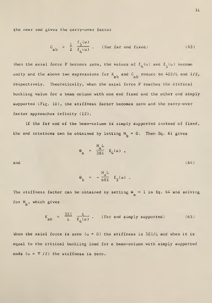
the near end gives the carry-over factor
Wh
1
f5(u)
C L = -. (For far end fixed) (63)
ab 2 f . lu)
en the axial force P becomes zero, the values of f,(u) and f c (u) become4 5
unity and the above two expressions for K , and C , reduce to 4E1/L and 1/2,ab ab
respectively. Theoretically, when the axial force P reaches the critical
buckling value for a beam column with one end fixed and the other end simply
supported (Fig. 10), the stiffness factor becomes zero and the carry-over
factor approaches infinity (12).
If the far end of the beam-column is simply supported instead of fixed,
the end rotations can be obtained by letting M = 0. Then Eq. 61 gives
M L
*a=
5il V u)'
and (64)
M L
9b
= " off V u) '
The stiffness factor can be obtained by setting 9 = 1 in Eq. 64 and solving£1
for M , which givesa &
3E1 1K , = —— -—;—
- . (Far end simply supported) (65)ab L f . (u) r
When the axial force is zero (u = 0) the stiffness is 3EI/L and when it is
equal to the critical buckling load for a beam-column with simply supported
ends (u = "FT /2) the stiffness is zero.

Fixed-end Moments
32
i 1 L
(a)
1 t i
(c) 9,
(d)
Fig. 11. Fixed-end beam with axial load.
The fixed-end moments can be obtained by superposing the solutions of
the problems shown in Fig. lib, c, and d. In order to cancel the effects of
the end rotations, moments must be applied at the ends. In Fig. lie, a
moment M ' is applied at the left end to rotate the axis of the member toa rr
the horizontal and the right end of the member is assumed to be held against
rotation thus, inducing a moment M, '. These two moments can be expressed as
M • = -K .9 •,a ab a

n
and
M, ' = M ' C ,= -K .C .9 '
.
b a ab ab ab a
In Fig. lid, the left end of the member is held against rotation and a
moment N is applied at the right end to remove the angle 9 . This gives
n i
b ba b
and
M " = M."
C, = -K u C L 9 '.
a b ba ba ba b
By superposing the results of Fig. lib, c, and d, the fixed-end moments are
M = M ' + M " = -K .9 '-K.C. 9 ',
a a a ababababand (66)
M, = M,' + M." = -K. 9 '-K C 9 .
b b b babababa
If the member is assumed to have constant cross-section, the stiffness and
carry-over factors at each end of the member will be the same and the above
expressions can be written as (12)
M = -K . (9 ' C . &. ') . and
a ab a ab b
(67)i
M, = -K . (9, C , 9 ) .
d ab b ab a
Uniform Load
For the case of a fixed-ended beam-column with a uniform load the
angles of rotation of the ends must be found for the simply supported beam-
column as shown in Fig. 2 and Eq. 10. These angles are
3
e -e. --ffer Mu) . (68)a b 24E1 2
34
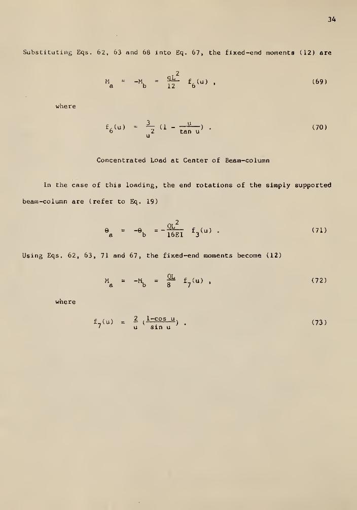
Substituting Eqs. 62, 63 and 68 into Eq. 67, the fixed-end moments (12) are
Ma
= A =
?T f6(u)
'(69)
where
f,(u) = ~ (1 - r-^— ) . (70)6 2 tan u
u
Concentrated Load at Center of Beam-column
In the case of this loading, the end rotations of the simply supported
beam-column are (refer to Eq. 19)
QL2
a b 16EI 3
Using Eqs. 62, 63, 71 and 67, the fixed-end moments become (12)
where
\ • -\ " * £7(U)
•<72>
£ (u , . 2(1=E2S_U)
. (73)' u sin u

35
Fixed-end Moments Due to Joint Translation
(a)
Fig. 12. Fixed-end moments due to joint translation.
By using the same procedures as in deriving "Fixed-end Moments" dis-
cussed above, the fixed-end moments due to joint translation shown in Fig.
12a can be obtained by superposing the results of Fig. 12b, c, and d. The
equations, which are necessary for this case, can be expressed as
= Kab I '
Mb
Kab
Cab L
;
" A ' Ab ba L a ba ba L

36
and
M«= M + M "
= (K , * K, C, ) 7 ,a a a ab ba ba L
M. = M, + M."
= (K. + K UC J 7 .
b b b ba ab ab L
(74)
If the member is of constant cross-section, the stiffness and carry-over
factors are the same at each end, and Eq. 74 is reduced to
MQ
= Mk " K k (1 c J 7 • (75)a b ab ab L
After substitution of the relationships given in Eqs . 62 and 63 for the
stiffness and carry-over factors, Eq. 75 becomes
M - m 6EIA ,,M
a " Mb
= ~T f8(u)
»
Li
where
2c , . u sin u t-,c\f Q (u) = ——, . (76)8 3(sin u - u cos u)
The same general procedure as for standard moment distribution, but
modified to make use of the superposition method, can be used in analyzing a
structure with sidesway.
Following the superposition technique of analysis, the moments in the
frames shown in Fig. 13a and b are determined first. The frame in Fig. 13b
is supported against joint translation and subjected to the same loads as
acting on the original frame. The frame in Fig. 13c is subjected to an
i
arbitrary horizontal displacement A and then held against further joint
translation. Both of these frames are analyzed by moment distribution con-
sidering the beam-column effect in the members. Therefore, it is necessary
to make an initial estimate of the axial forces in each member.

37
T*TTT"»
J_JP
3 1
TTTTrf
(a)
rhrrt
LAr4- R°i i-*' i r/
///»*»
(b) (c)
Fig. 13. Rigid frame with sidesway.
This estimate, which can be made by an approximate analysis of the original
structure, gives a value of the factor "kL" for each member of the frame,
and the factor "kL" is held constant throughout the analyses of the frames
shown in Fig. 13b and c. The superposition equations to be used are the
same as in the standard moment distribution calculations. For the notations
shown in Fig. 13, the equation
R° - aR =0
determines the constant of proportionality "a" and the equation
M = Mu + aM
(77)
(78)
determines the moments M in the original structure, assuming that M° and M
represent moments in the frames of Fig. 13b and c, respectively. After
determining the moments in the original frame, the values of the axial
forces in the members are revised to more accurate values and the entire
process repeated if necessary.

38
DESIGN METHODS
Two simple approximate methods have been developed for estimating the
strength of beam-columns. The first method, generally referred to as the
secant formula method, is based upon the concept that the load which pro-
duces initiation of yielding in the fibers subjected to maximum stress
provides a lower bound to the failure load. The second method is to consider
the member as a cross between a beam under pure bending and a column under
pure axial load, its two limiting cases (13).
SECANT FORMULA METHOD
As stated above, the secant formula method specifies that the maximum
stress in the beam-column, modified by a factor of safety, may not exceed
the yield stress of the material. The formulas developed for this procedure
apply only to members that fail by bending in the plane of the applied
loads. The procedure applies best for material having a linear elastic
stress-strain relationship.
^"Fp
(a)
P
(b)
X
1
1J
1 1
1 k
eb
Fig. 14. Notation for eccentrically loaded members

39
The first step in developing the secant formula is the analysis of
maximum combined stress produced by axial load, applied bending moment, and
bending moment due to deflection. Consider the case of two eccentrically
applied compressive forces P with unequal eccentricities as shown in Fig.
14b, the deflection curve has been derived in Eq. 23.
sin k(L-x) L-x . s_i_n_kx xy = e l ;
~— - —— ) + e. (—" — - ~), (23)
a sin kL L b sin kL L
in which e denotes the larger eccentricity and e , the smaller one.
e bBy letting t = —
, the deflection curve is reduced toea
.t-coskL. , . 1-t ,, ,__.
y = e ( :
~ sin kx + cos kx ~— x - 1) . (79)J a sin kL L
Substituting Eq. 79 into Eq. 21a, we find that the expression for bending
moment at any section in the member, after some rearrangement, is
™ r t — cos kL , ,i /o«nM = P e I;— sin kx + cos kxj . (80)
a sin kL J
Taking the first derivative of M with respect to x and setting dM/dx , we
find the location of the maximum moment as
1 t - cos kLx = r arc tan ;
—.
k sin kL
Substituting this back into Eq. 80, after some manipulation we obtain the
maximum moment,
1^M P e (
C - a C°f
kL + L) . (81)
max a sin kL
The maximum fiber stress in the member is equal to

40
p M cf _ maxmax A 1
£ - f a.* ¥ Vt2 - 2t c
:rkL^ . <62>mnx A 2 sin kL
r
where c i6 the distance from the neutral axis to the extreme fiber in com-
pression. It is this stress which is to be set equal to the yield point
stress f to determine the yield point load P , thusy y
fy_ + f£ //t2
- 2t cos kL.±_l m f . (83)A 2 sin kL y
r
The limiting average stress F for design use can be obtained from Eq. 83 byfit
replacing P with nF A (where n is the factor of safety) and then solving
for F , thusa
f /nY
. (84)
2/~~2
1 + e c/r // t - 2t cos kL + 1 esc kLa
In Appendix C of the AASHO Specifications (1965 edition) we find formula A,
which is almost identical with Eq. 84
f /np
fs
= S 7 " I * (85)
1 (0.25 + e c/r ) B cosec 6a T
where B is the factor similar to r/t - 2t cos kL + 1 and <}> replaces kL.
2The term 0.25 which is added to the nondimensional factor e c/r is to
a
account for the effects of all imperfections, such as initial crookedness,
nonhomogeneity , and residual stress.
Equations 84 and 85 are quite difficult to use for design, and their

41
main use is in plotting column curves such ns those in Appendix C of the
AASHO Specifications. Such curves ore reasonably easy to use for the trial
and error design of beam columns.
For the particular case in which the eccentricity of the load is a con-
stant value e, we set t = 1, and after some slight manipulation Eq. 82
reduces to the well-known secant formula:
c P [ ec kL-,, _, ,
f = r [1 + -r sec —J , (86)max A 2 2 J
r
and the corresponding expression for allowable stress for design use is
f /n
F = r* . (87)a
1 (ec/r ) sec (kL/2)
The secant formula suggested by Column Research Council (7) is
e c i
—f = 7 [1 + (^ + -^r-) sec £- /fr] , (88)max A 2 2 2r n AEJ
r r
and the corresponding expression for allowable stress is
f /nJt
1 + (ec/r + e c/r ) sec (L/2r) JnV /E
F«
=:
—
—2 V'o
where e is the assumed equivalent eccentricity representing the effects of
all defects.
A good approximation for the maximum moment in a beam-column can be
found from the following equation:
PAM = M * 1
^~~»
(90)max o 1 - P/P
cr
where M and A are the moment and deflection, respectively, without regard

42
to the added moment caused by deflection. Eq. 90 can conveniently be
written as:
1 + vj; P/PMmax
= M (
cr6 1- P/P ) ,
cr(91)
in which, for a simply supported constant-section member,
F £ El
* = °— " 1 •
M Lo
If the approximate maximum moment given by Eq. 91 is used to determine the
maximum combined stress in a beam-column, the following formula is obtained
maxI .
f
l + *<X Mo°
A 1 - 0( ' 1(92)
where o< = P/Pcr
Since formulas for lateral deflection A under different loading conditionso
are available in handbooks, Eq. 92 greatly simplifies calculation of maximum
stress in beam-columns. Several values of ^ for various conditions are
given (7) in Table 2.
Table 2. Parameter <\j in Eqs. 91 and 92.
Loading condition
Constant moment + 0.233
Concentrated lateralload at midspan - 0.178
Uniform lateral load + 0.028
7*
Each loading condition shown in Table 2 is assumed to act simultaneously
with axial compression forces.

43
If Eq. 92 is used for the same design case as that of Eq. 90 (equal
eccentricities e, M - Pe, and ^ ~ + 0.233), the allowable stress becomes
f /nF - ^ (93)a
,1 + 0.233ntx , ec *
1 + (
1 - nC*}
2r
This equation gives results in close agreement with those obtained from Eq
,
89. The results are within IV. for nc* less then 0.8, and within 2.5/, for
0.8 < ncx < 0.95 (7).

44
INTERACTION FORMULA METHOD
This method is based on the use of interaction formulas for beam-
columns subjected to bending in the weak direction, and for beam-columns
subjected to strong-direction bending provided that they are adequately
braced against lateral buckling. Interaction formulas have a simple form,
are convenient to use, and have a wide scope of application. Allowable
stresses determined from interaction formulas vary continuously and in a
smooth transition from stresses for concentrically loaded columns at one
limit to stresses for beams at the other. Formulas for combined stresses
used in AISC Specifications are based on this method.
The strength of members subjected to bending combined with compression
forces can be expressed conveniently by interaction formulas in terms of
the ratios P/P and M/M , whereu u
P = compression forces at actual failure,
P = ultimate load for the centrally loaded column for buckling in the
plane of the applied moment,
M = maximum bending moment at actual failure, and
M = ultimate bending moment in the absence of axial load,u °
The following equation is the basis for several such interaction formulas:
§-«-« i.u u
In the elastic range, an approximation of the maximum bending moment
for beam-columns subjected to combined bending and compression producing
maximum moment at or near the center of the member may be obtained from Eq.
91 by setting ty= 0.

45
M
Mmax
=1 - (P/P )
'(95)
cr
where P = applied axial load,
P = elastic critical load for buckling in the plane of appliedmoment, and
M = maximum applied moment, not including contribution of axialload interacting with deflections.
Substituting Eq. 95 into Eq. 94 gives
M1 1 . (96)
P M 1- (P/P )Ju u cr
For eccentrically loaded columns having equal end eccentricities e at both
ends, Eq. 96 may be expressed as
P P e— + — t - 1 (97)P M [1 - (P/P )Ju u cr
Galambos and Ketter (4) presented dimensionless interaction curves for
the ultimate strength of typical wide-flange beam-columns bent in the strong
direction and having (a) equal axial-load eccentricities at both ends, and
(b) eccentricity at one end only. The parameters used for the maximum-
strength formulas are P/P and M/M , and the interaction formulas take they U
following form:
M P P 2A— *B — + C(— ) * 1 , (98)
u y y
where A, B, and C are empirical coefficients that are functions of L/r and
of loading conditions, and P is the column axial load at the fully yielded
condition (P = A f ).y y
The A1SC Specifications (14) use a complete tabulation of the

46
Galambos-Kcttcr coefficients of Eq . 98 for beam columns loaded as described
in the preceding paragraph.
For the case of strong-direction bending, where a beam-column is bent
in double curvature by moments producing plastic hinges at both ends, the
A1SC recommends a strength formula that can be written as
M
p y
This equation is independent of L/r, and M is the plastic moment
(M = Z f , where Z is the plastic modulus).P y
For designing a beam-column subjected to unequal end moments, it may be
over conservative to use the maximum of these in an interaction formula for
design of the member, especially where the end moments are of opposite sign.
This is because the interaction formula assumes the maximum moment to be at
or near the center of the span. The AISC Specifications present an approx-
imate expression of "equivalent uniform moment," which can be expressed as
follows
:
M M
ZT9
- - 0.6 + 0.4 r* * 0.4 , (99)M Ma a
where M is the equivalent uniform moment, and M, /M is the ratio of theeq b a
smaller to larger moments at the ends of the member.
In AISC specifications section 1.6.1. the interaction equations are in
the form
f C f K
f+ ^ * i ,(100)
a(1 - ~) FKl
F' be

Isi
and
f £ K-* * 1 , (101)
O.o F 1,y b
where f and f, are the axial and bending stresses under the combined load-a b
ing, F and F, are the allowable stresses for the axially loaded column and° a b J
beam, respectively, F' is the critical stress according to Euler's column
theory, and C is a coefficient which is expressed as
C = 0.6 + 0.4 (M./M )2 0.4 .
m b a
In the case of biaxial bending, the design interaction equation is
written as
f C f K C f K_§. +
mx bx my bY ± i (102 )
F (1 - f /F' ) i\ (1 - f /F' ) F ul
'^ 1UZ;
a a ex bx a ey by
where the subscripts, x and y, refer to the x and y axes.
The great usefulness and versatility of interaction formulas arises
from the possibility of including a variety of conditions in at least an
approximate manner. For instance, if the danger of lateral buckling under
applied moment exists, the allowable stress F, can be reduced accordingly.
Interaction formulas also allow consideration of end effects such as
partial or complete fixity, or sideway. A member with these end effects can
be designed safely by replacing the restrained beam-column by an equivalent,
hinged-end beam-column having a length equal to the effective length of the
real, restrained beam-column, and analyzing this equivalent beam-column for
axial compression.
An example illustrating the interaction formula concept is presented in
the following section.

48
EXAMPLE
P ro b 1 em :
A column in a steel building frame is, according to an analysis, sub-
jected to an axial force of 300 kips and a moment of 200 k-ft at the lower
end, 150 k-ft at the upper end. There is no moment about the other axis,
and the frame is braced against sidesway buckling in the plane of the load-
ing and in the plane perpendicular to it. Story height is 18 ft. Use A-36
steel and design the member according to AISC Specifications (14).
300 k.
18 ft
200 k-ft.
300 k.
Solution
:
For a quick estimate of the range of member size, consider the moment
of 200 kip-ft alone, and compute the required section modulus as
req F.
200 x 12
22109 in
3,
Assume that, owing to the presence of axial force, twice this value
3is reasonable and look for a member with section modulus of about 200 in .
Entering the Tables on pages 1-12 (AISC), the 14 \F shapes are found to be

49
suitable for this size. Accordingly, consider a 14 IF 127, for which
A = 37.33 in2
,
S = 202.0 in,
1 = 1476.6 in4
,
r =6.29, andx
r = 3.76.y
Since sidesway buckling is prevented, assume that the effective length
factor K to be 0.65 according to Table C. 1.8.2.
On the basis of these data calculate the slenderness ratios:
L 18 x 12 _. . L 18 x 12 e_ .
T ="6T2T~
= 34 ' 4 7"= T^6~ = 57 - 5
•
x y
Effective slenderness ratios:
— = 0.65 x 34.4 = 23 ,rx
— = 0.65 x 57.5 = 38 .
ry
Allowable axial stress:
(Table 1-36)
F = 20.41 ksi ;ax
F = 19.35 ksi .
ay
Axial stress:
f _ I - 300 . A , ..

50
Reduction factor:
MCm
0.6 + 0.4 (^) = 0.6 + 0.A (^§§) = 0.3 < 0.4,
use C = 0.4m
Amplification factor:
— = 23 , F 1 = 281.88 ksi ,
rx
F' 281.88U,y/1
*
e
Allowable bending stress: (sec. 1.5.1.4.5)
Fu = !^/?°° = 56 ksi > 0.6 F , use F, =0.6 F = 22 ksib Ld/A
f y b y
Bending stress:
Mc max _ 200 x 12 . , QO . .
fb
= T" " "202= U * 88 kSl *
Check interaction formulas:
a 8 04
F=
1935= °* 416> °' 13
»use Formula ( 7).
a
Formula (7a)
-8-^+ °' 4 (1I ' 88 > = 0.416*0.222 = 0.638< 1 .
19.35 0.971 (22)^
Formula (7b)
8.04 . 11.8822 22
= 0.366 + 0.54 = 0.906< 1.0 .
51
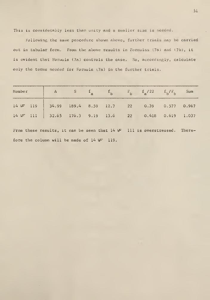
This is considerably less than unity and a smaller size is needed.
Following the same procedure shown above, further trials may be carried
out in tabular form. From the above results in Formulas k7&> and l7b;, it
is evident that Formula (7a) controls the case. vSo , accordingly, calculate
only the terms needed for Formula v7a) in the further trials.
Member f /22 f u/Fu Suma b b
14 \F 119
14 UF 111
34.99 189.4 8.59 12.7 22
32.65 176.3 9.19 13.6 22
0.39 0.577 0.967
0.418 0.619 1.037
From these results, it can be seen that 14 UF 111 is overstressed . There-
fore the column will be made of 14 VF" 119.

52
CONCLUSION
The foregoing material demonstrates the means of analysis and design of
beam-columns. In addition to the four methods for the analysis of the
behavior of beam-columns discussed above, there are many other methods for
solving a beam-column problem.
The general method which is derived on the basis of the differential
equations of beam-columns gives a theoretical and "exact" solution of the
problem. From a practical viewpoint, a large number of laterally applied
loads or changes in section leads to a solution by the general method which
is probably no more precise or applicable than the solution obtained by one
of the approximate methods.
The energy method uses a single mathematical expression for the assumed
deflection which holds for the entire length of the beam. With this method
it is not necessary to discuss separately each portion of the deflection
curve between consecutive loads, yet it gives a good approximate solution
for the problem. This method of analysis is especially useful in the case
of a member with simply supported ends, of a member with complicated load-
ings, and of a member with various cross-sections.
The numerical method is also an approximate method with a high degree
of accuracy. The problem that can be solved by using the numerical proce-
dure as described is almost unrestricted by the type of loading.
The basic principle of the general method may be extended to solve
rigid frame problems by using the modified moment distribution method.
The expression for the secant formula is complicated in form and is
quite difficult to use for design. The main purpose of the secant formula
is to plot column curves such as shown in the AASHO Specifications (15).

53
Such curves are reasonably easy to use for the design of bcara-columna by
trial and error.
The interaction formula is easy to use for design and is applicable for
a variety of loading conditions.

34
ACKNOWLEDGMENTS
The writer wishes to express his deepest appreciation and gratitude
to his major instructor, Professor Vernon H. Rosebraugh, whose guidance,
criticism, and most helpful suggestions in regard to the technical problems
involved rendered this report possible.

55
NOTATION
a, b, c, d Numerical coefficients, distances
A Cross-sectional area
c Distance from neutral axis to extreme fiber of beam
e , e, , e Eccentricitya b J
E iModulus of elasticity
f (u), f (u) Amplification factors for beam-columns
1 Moment of inertia
k Axial load factor for beam-column
K Stiffness factor, effective length factor
L Length, span
m, n Integers, numerical factors
M Bending moment, couple
M , M, Bending moments at end A and B, respectively
n Factor of safety
P Axial force in beam-column
P Critical buckling loadcr 6
Q Concentrated force
q Intensity of distributed load
r Radius of gyration
R Shearing force in conjugate beam
o •
R , R Reactive force
s Horizontal displacement, distance
S Section modulus
t Numerical ratio
T Work, tension force

56
u Axial load factor for beam-columns (u = kL/2)
U Strain energy
V Shearing force in beam
x, y Rectangular coordinates
y',y"... First derivative, second derivative, etc.
Z Plastic modulus
c< Numerical factor, ratio
L Deflection
e , e. End slopes, rotationsa b r
<\> Numerical factor

57
BIBLIOGRAPHY
1. "Numerical Procedure for Computing Deflections, Moments and BucklingLoads," N. M. Newmark, Trans . ASCE Vol. 108 (1943), p. 1161.
2. Buckling Strength of Metal Structures . F. Bleich, McGraw-Hill, NewYork, 1952.
3. "Plastic Deformation of Wide-Flange Beam Columns," R. L. Ketter, E. L.
Kaminsky, and L. S. Beedle, Trans . ASCE Vol. 120 (1955), p. 1028.
4. "Column Under Combined Bending and Thrust," T. B. Galambos and R. L.
Ketter, Trans . ASCE Vol. 126 Part 1 (1961), p. 1.
5. "Further Studies of the Strength of Beam-columns," R. L. Ketter, Trans .
ASCE Vol. 126 Part 2 (1961), p. 929.
6. "Eccentrically Loaded, End -res trained Columns," P. 0. Bijlaard, G. P.
Fisher, G. Winter, and R. E. Mason, Trans . ASCE Vol. 120 (1955),p. 1070.
7. Guide to Design Criteria for Metal Compression Members , B. G. Johnston,Column Research Council, John Wiley & Sons, New York, 1966.
8. Theory of Elastic Stabi lity , S. P. Timoshenko, and J. M. Gere, McGraw-Hill, New York, 1961.
9. Structural Mechanics . S. T. Carpenter, John Wiley 6. Sons, New York,
1960.
10. Numerical and Matrix Methods in Structural Mechanics . P. C. Wang, JohnWiley & Sons, New York, 1966.
11. Numerical Analysis of 3eam and Column Structures , W. G. Godden,Prentice-Hall, New Jersey, 1965.
12. Moment Distribution , J. M. Gere, D. Van Nostrand Company, New Jersey,1963.
13. Basic Structural Design . K. H. Gerstle, McGraw-Hill, New York, 1967.
14. Manual of Steel Construction . American Institute of Steel Construction,1963.
15. Standard Specifications for Highway Bridges . American Association ofState Highway Officials, 1965.

ANALYSIS AND DESIGN OF BEAM-COLUMNS
by
CHENG-HSIUNG CHEN
Diploma, Taipei Institute of Technology, 1959
AN ABSTRACT OF A MASTER' S REPORT
submitted in partial fulfillment of the
requirements for the degree
MASTER OF SCIENCE
Department of Civil Engineering
KANSAS STATE UNIVERSITYManhattan, Kansas
1967

Beam-columns arc members which are subjected to combined bending and
axial compression. The bending may arise from lateral loads, couples
applied at any point on the beam, or from end moments caused by eccentricity
of the axial loads at one or both ends of the member.
The purposes of this paper are to review the appropriate methods for
analyzing beam-column problems, namely, the general method, the energy
method, the numerical method, and the moment distribution and to discuss
adequate procedures for designing steel beam-columns.
The general method or "exact" method is based on the relationship
between moment and curvature of a beam, Ely" = -M, and takes into account
the compressive forces. By solving this differential equation with known
boundary conditions, the maximum deflection and moment can be obtained.
The energy method is widely used in the field of structural mechanics,
and represents a unique mathematical application of the basic law of con-
servation of energy. By assuming the elastic curve to be described by,
y = L & sin(n~ x/L), the external work done by physically applied external
forces or moments may be set equal to the potential energy stored through
the action of the internal forces and the elastic strain mechanisms of the
beam-column. The coefficients "a " can be determined, and the maximumn
moment obtained.
The numerical method was first presented by N. M. Newmark. It provides
a means of obtaining an approximate solution for beam-columns with complex
loading.
The theoretical principle of the general method can be extended to
calculate the modified stiffness and carry-over factors for use in the method
of modified moment distribution. The modified moment distribution method

can then be used to solve rigid frame problems.
Two approaches to the design of steel beam-columns are described in
this paper. Criteria for these methods are the CRC (Column Research
Council) design guide (7), AASHO (15), and A1SC (14) Specifications. Three
sample problems are analyzed and one design example is given to illustrate
the design procedure according to the A1SC Specifications.