Embed Size (px)
Citation preview

American Journal of Engineering Research (AJER) 2019
American Journal of Engineering Research (AJER)
e-ISSN: 2320-0847 p-ISSN : 2320-0936
Volume-8, Issue-8, pp-40-53
www.ajer.org Research Paper Open Access
w w w . a j e r . o r g
w w w . a j e r . o r g
Page 40
Analysis and Comparative Study of Numerical Solutions of Initial
Value Problems (IVP) in Ordinary Differential Equations (ODE)
With Euler and Runge Kutta Methods
Anthony Anya Okeke 1,*
, Pius Tumba1, Onyinyechi Favour. Anorue
2, Ahmed
Abubakar Dauda1
1 Department of Mathematics, Federal University Gashua, P.M.B. 1005 Gashua, Yobe State, Nigeria
2 Department of Mathematics, Michael Okpara University of Agriculture, Umudike, Abia State, Nigeria
Corresponding Author: Anthony Anya Okeke
ABSTRACT : In this paper, we present Euler’s method and fourth-order Runge Kutta Method (RK4) in solving
initial value problems (IVP) in Ordinary Differential Equations (ODE). These two proposed methods are quite
efficient and practically well suited for solving these problems. For us to obtain and verify the accuracy of the
numerical outcomes, we compared the approximate solutions with the exact solution. We found out that there is
good agreement between the exact and approximate solutions. We also compared the performance and the
computational effort of the two methods. In addition, to achieve more accuracy in the solutions, the step size
needs to be very small. Lastly, the error terms have been analyzed for these two methods for different steps sizes
and compared also by appropriate examples to demonstrate the reliability and efficiency.
KEYWORDS Ordinary Differential Equations (ODE), Initial value Problems (IVP), Euler Method, Runge Kutta
Method, Error Analysis.
----------------------------------------------------------------------------------------------------------------------------- ----------
Date of Submission: 20-07-2019 Date of Acceptance: 06-08-2019
----------------------------------------------------------------------------------------------------------------------------- ----------
I. INTRODUCTION It is a common truth that Differential Equations are among the most important Mathematical tools used
in producing models in the engineering, mathematics, physics, aeronautics, elasticity, astronomy, dynamics,
biology, chemistry, medicine, environmental sciences, social sciences, banking and many other areas [1]. Many
researchers have studied the nature of Differential Equations and many complicated systems that can be
described quite precisely with mathematical expressions. A differential equation that has only one independent
variable is called an Ordinary Differential Equation (ODE), and all derivatives in it are taken with respect to that
variable. Most often, the variable is time, t; although, some authors use x as the independent variable. The
differential equation where the unknown function depends on two or more variables is referred to as Partial
Differential Equations (PDE). Although there are many analytic methods for finding the solution of differential
equations, there exist quite a number of differential equations that cannot be solved analytically [2]. This means
that the solution cannot be expressed as the sum of a finite number of elementary functions (polynomials,
exponentials, trigonometric, and hyperbolic functions). For simple differential equations, it is possible to find
closed form solutions [3]. But many differential equations arising in applications are so complicated that it is
sometimes impractical to have solution formulas; even when a solution formula is available, it may involve
integrals that can be calculated only by using a numerical quadrature formula. In either case, numerical methods
provide a powerful alternative tool for solving the differential equations under the prescribed initial condition or
conditions [3].
There are many types of practical numerical methods for solving initial value problems for ordinary
differential equations. Historically, the ancestor of all numerical methods in use today was developed by
Leonhard Euler between 1768 and 1770 [4], improved Euler’s method and Runge Kutta methods described by
Carl Runge and Martin Kutta in 1895 and 1905 respectively [5]. We have excellent and exhaustive books on this
can be consulted, such as [1-3, 6-15]. In this work, we shall consider two standard numerical methods Euler and
Runge Kutta for solving initial value problems of ordinary differential equations.
American Journal of Engineering Research (AJER) 2019
w w w . a j e r . o r g
w w w . a j e r . o r g
Page 41
From the literature review, we found that many authors have worked on numerical solutions of initial
value problems using the Euler method and the Runge Kutta method. Many researchers have attempted to solve
initial value problems to get a higher accurate solution by applying numerous methods, such as the Euler
method and the Runge Kutta method, and many other methods. In [16], the authors studied on some numerical
methods for solving initial value problems in ordinary differential equations and also in [17],the authors
presented Euler’s method for solving initial value problems in ordinary differential equations. Islam
[18]discussed accurate solutions of initial value problems for ordinary differential equations with the fourth
order Runge Kutta method, while [19] discussed accuracy analysis of numerical solutions of initial value
problem for ordinary differential equations. [20-24]also studied numerical solutions of initial value problems in
ordinary differential equations using different numerical techniques. In this paper, Euler’s method and fourth
order Runge Kutta methods are applied without discretization, transformation or restrictive assumptions for
solving initial value problems in ordinary differential equations.
Euler’s method historically is the first numerical technique. It is also called the tangent line method. It
is the simplest to understand and geometrically easy to articulate. The method needs to take a smaller value of h,
because of this restriction the method is unsuitable for practical use. If h is not small enough, this method is too
inaccurate. A rigorous and elaborate numerical technique is the Runge Kutta method. This technique is the most
widely used one since it gives starting values and is particularly suitable when the compilation of higher
derivatives is complicated [19]. The numerical results are very encouraging.
Finally, we used two examples to illustrate the proposed formulae. The results obtained from each of
the numerical examples show that the convergence and error analysis which we presented clearly illustrate the
efficiency of the methods. In general, each of the numerical methods has its own advantages and disadvantages
to use. Euler’s method requires less time consumption, it is simple and single step. Also, in Euler’s method dy
dx
changes rapidly over an interval, this gives a poor approximation at the beginning of the process in comparison
with the average value over the interval. So the calculated value of y in this method occurs much error than the
exact value, which reasonably increased in the succeeding intervals, then the final value of y differs on a large
scale than the exact value.
In fact, Euler’s method needs to take a smaller value of h, and as such, the method is suitable for
practical use. If h is not too small enough, this method is inaccurate. But, the Runge Kutta method has the
advantage of being the most widely used numerical weapon, since it gives reliable values, starting values and
particularly suitable when the computation of higher order derivatives are complicated. It gives a greater
accuracy than the Euler’s method and also possesses the advantage of requiring only the function values at some
selected points on the sub-intervals. Moreover, it is easy to change step-length for special procedures necessary
for starting, which minimize the computing time. The Runge Kutta method is very useful and also very
laborious. It is a lengthy procedure and needs to check back the values computed earlier. The inherent error in
the Runge Kutta method is hard to be estimated and the method has its limitation in solving certain types of
differential equations only and the step-length is the key factor of the computation.
Lastly, this paper is structured as follows: Section 2: problem formulations; Section 3: numerical examples;
Section 4: discussion of results; and the last section, the conclusion of the paper.
II. PROBLEM FORMULATION In this section, we consider two numerical methods for finding the approximate solutions of the initial value
problem (IVP) of the first order ordinary differential equation of the form
y′ = f x, y , x ∈ a, b , y a = y0 (2.1)
Where y′ =dy
dx and f(x, y) is a given function and y(x) is the solution of the equation (2.1).
Theorem 2.1 [1]
Let f(x, y) be defined and continuous for all points (x, y) in the region D defined by a ≤ x ≤ b, −∞ < y < ∞, a
and b finite, and let there exist a constant L such that, for every x, y, y∗, such that (x, y) and (x, y∗) are both in D,
|f x, y − f(x, y∗) ≤ L(y − y∗)|. (2.2)
Then, if y0 is any given number, there exists a unique solution y(x) of the initial value problem (2.1), where
y(x) is continuous and differentiable for all (x, y)in D.
In this paper, we determine the solution of this equation in the range a ≤ x ≤ b, where a and b are finite, and we
assume that f satisfies the Lipchitz conditions stated in Theorem 2.1.
A continuous approximation to the solution y(x) will not be obtained; instead, an approximation to y
will be generated at various values. Called mesh points, in the interval a ≤ x ≤ b. Numerical techniques for the
solution of (2.1) is to obtain approximations to the values of the solution corresponding to the sequence of points xn defined by xn = a + nh, n = 0, 1, 2, 3, ….The parameter h is called the step size. The numerical solution of
(1) is given by a set of points { xn , yn : n = 0, 1, 2, 3, … , N} and each point (xn , yn ) is an approximation to the
corresponding point (xn , y(xn)) on the solution curve.

American Journal of Engineering Research (AJER) 2019
w w w . a j e r . o r g
w w w . a j e r . o r g
Page 42
2.1.1. Euler’s Method
Euler’s method is also called the tangent method and it is the simplest one-step method. It is the most
basic example method for numerical integration of ordinary differential equations. The Euler method is named
after Leonhard Euler, who treated it in his book Institutiones Calculi Integralis published 1768-1870,
republished in his collected works (Euler 1913) [2]. The Euler method is subdivided into three namely:
Forward Euler’s method
Improved Euler’s method
Backward Euler’s method
In this paper, we shall only consider the forward Euler’s method.
1.1.1. Derivative of Euler’s Method
Let us consider the initial value problem
y′ =dy
dx= f x, y ; y x0 = y0 (2.3)
We know that if the function f is continuous in the open interval a < x < bcontaining x = x0, there exists a
unique solution of the equation (2.3) as
yn = y xn ; n = 1, 2, 3, … (2.4)
The solution is valid for throughout the interval a < x < b. We wish to determine the approximate value of yn
of the exact solution y = y(x) in the given interval for the value x = xn = x0 = nh; n = 0, 1, 2, ….Now, the
equation of the tangent line through (x0, y0) of (3) is
y x = yn + f(x0, y0) x − x0 , Setting x = x1, we have
y1 = y0 + hf(x0, y0), Similarly, we get the next approximation as
y2 = y1 + hf x1, y1 , atx = x2
y3 = y2 + hf x2, y2 , atx = x3
In general, the (n + 1)th approximation at x = xn+1 is given by
yn+1 = yn + hf xn , yn ; n = 0, 1, 2, 3, … (2.5)
1.1.2. Truncation Error for Euler’s method
Numerical stability and errors are well discussed in depth in [10, 12-14]. There are two types of errors
in the numerical solution of ODEs: Round-off errors and truncation errors. Round-off error occurs because
computers use a fixed number of bits and hence fixed the number of binary digits to represent numbers. In a
numerical computation round-off errors are introduced at every stage of computation. Hence though an
individual round-off error due to a given number at a given numerical step may be small but the cumulative
effect can be significant. When the number of bits required for representing a number is less than the number is
usually rounded to fit the available number of bits. This is done either by chopping or by symmetric rounding.
Also, truncation errorarises when you use an approximation in place of an exact expression in a mathematical
procedure. To estimate the truncation error for the Euler method, we first recall Taylor’s Series approximation
of a function.
Essentially, Taylor’s Theorem State, that, any smooth function can be approximated by a polynomial. The
Taylor Series Expansion of f(x) at a is
f x = f a + f ′ a x − a +f ′′ a x − a 2
2!+
f ′′′ a x − a 3
3!+ ⋯
= f n a x − a n
n!
∞
n=0
(2.6)
We note that computers are discrete, finite machine. They can’t perform infinite calculation like these, so we
have to cut the calculation somewhere. This result in truncation error (we truncate the expression). When we
truncate the Taylor’s Series expression to n terms, there’s error left over, and we can include a remainder tern
Rn to keep the = sign exact.
f x = f a + f ′ a x − a +f ′′ a x−a 2
2!+
f ′′′ a x−a 3
3!+ ⋯ +
f n a x−a n
n!+ Rn (2.7)
Where Rn =f(n +1) ζ .hn +1
n+1 !, andx ≤ β ≤ a.
In (2.7), let x = xn+1 and x = a, in which
y xn+1 = y xn + hy′ xn +1
2h2y′′(βn ) (2.8)
Since y satisfies the ordinary differential equation (3), which can be written as
y′ xn = f(xn , y xn ) (2.9)
Hence,’

American Journal of Engineering Research (AJER) 2019
w w w . a j e r . o r g
w w w . a j e r . o r g
Page 43
𝑦 𝑥𝑛+1 = 𝑦 𝑥𝑛 + ℎ𝑓 𝑥𝑛 , 𝑦(𝑥𝑛) +1
2ℎ2𝑦′′(𝛽𝑛) (2.10)
By considering (2.10) to Euler’s approximation in (2.5), it is very clear that Euler’s method is obtained by
omitting the remainder term 1
2ℎ2𝑦′′(𝛽𝑛) in the Taylor’s expansion of 𝑦(𝑥𝑛+1) at the point 𝑥𝑛 . Therefore, the
truncation 𝑇𝑛+1 error is given by
𝑇𝑛+1 = 𝑦 𝑥𝑛+1 − 𝑦 𝑥𝑛 = ℎ𝑦′(𝑥𝑛) +1
2ℎ2𝑦′′(𝛽𝑛) (2.11)
Thus, the truncation error is of 𝛰 ℎ2 : ℎ ⟶ 0, i.e. the truncation error is proportional to ℎ2. By diminishing the
size h, the error can be minimized. If 𝑀 is positive constant such as 𝑦′′(𝑥) <𝑀
2
𝑇𝑛+1 <𝑀ℎ2
2 (2.12)
Here the right hand size is an upper bound of the truncation error. The absolute value of 𝑇𝑛+1 is taken for the
magnitude of the error only.
1.2. Runge Kutta Method
Runge Kutta method is a technique for approximating the solution of ODEs. This technique was
developed by two German Mathematicians, Karl Runge by 1894 and extended by Wilhelm Kutta a few years
later. The technique is popular because it is efficient, quite accurate, stable, and used in most computer
programmes for differential equations. The Runge Kutta methods are distinguished by their order in the sense
that they agree with Taylor’s series solution up to terms of ℎ𝑟 , where 𝑟 is the order of the method. It does not
demand prior computational of higher derivatives of 𝑦(𝑥) as in Taylor’s series method. The under-listed are the
order of the Runge Kutta Method:
Runge Kutta Method of order one is called Euler’s Method,
Runge Kutta Method of order two is the same as modified Euler’s or Heun’s Method,
The fourth order Runge Kutta Method is called Classical Runge Kutta Method.
In this paper, we shall only focus on the fourth order Runge Kutta Method.
1.2.1. The Derivative of the Fourth Order Runge Kutta method
We shall derive the formula of fourth order Runge Kutta method to obtain an approximate numerical solution of
the first order differential equation 𝑦’ = 𝑓(𝑥, 𝑦) with the initial condition 𝑦 𝑥0 = 𝑦0 and it is assumed that is
not a singular point.
Let us take the first order differential equation
𝑦′ =𝑑𝑦
𝑑𝑥= 𝑓 𝑥, 𝑦 ; 𝑦 𝑥0 = 𝑦0 (2.13)
Let ℎ = 𝑥1 − 𝑥0, from Taylor’s series expansion, we have
𝑦 𝑥 + ℎ = 𝑦 𝑥 + ℎ𝑦′ 𝑥 +ℎ2
2!𝑦′′ 𝑥 +
ℎ3
3!𝑦′′′ 𝑥 + ⋯
or𝑦 𝑥 + ℎ − 𝑦 𝑥 = ℎ𝑦′ 𝑥 +ℎ2
2!𝑦′′ 𝑥 +
ℎ3
3!𝑦′′′ 𝑥 + ⋯ (2.14)
Differentiating (2.1) partially with respect to variables 𝑥&𝑦 , we get
𝑦′ = 𝑓 𝑥, 𝑦 = 𝑓
𝑦′′ = 𝑓 ′ 𝑥, 𝑦 = 𝑓𝑥 + 𝑓𝑓𝑦
𝑦′′ = 𝑓 ′′ 𝑥, 𝑦 = 𝑓𝑥𝑥 + 2𝑓𝑓𝑥𝑦 + 𝑓2𝑓𝑦𝑦 + 𝑓𝑥𝑓𝑦 + 𝑓𝑓𝑦2
𝑦𝑖𝑣 = 𝑓 ′′′ 𝑥, 𝑦 = (𝑓𝑥𝑥𝑥 + 3𝑓𝑓𝑥𝑥𝑦 + 𝑓2𝑓𝑥𝑦𝑦 + 𝑓3𝑓𝑦𝑦𝑦 + 𝑓𝑦 𝑓𝑥𝑥 + 2𝑓𝑓𝑥𝑦 + 𝑓2𝑓𝑦𝑦 + 3 𝑓𝑥 + 𝑓𝑓𝑦 𝑓𝑥𝑦 + 𝑓𝑓𝑦𝑦
+ 𝑓𝑦2(𝑓𝑥 + 𝑓𝑓𝑦)
Let us introduce the following convenient form
𝐹1 = 𝑓𝑥 + 𝑓𝑓𝑦 , 𝐹2 = 𝑓𝑥𝑥 + 2𝑓𝑓𝑥𝑦 + 𝑓2𝑓𝑥𝑦 , 𝐹3 = 𝑓𝑥𝑥𝑥 + 3𝑓𝑓𝑥𝑥𝑦 + 𝑓2𝑓𝑥𝑥𝑦 + 𝑓2𝑓𝑦𝑦𝑦
Then we get as
𝑦′ = 𝑓, 𝑦′′ = 𝐹1, 𝑦′′′ = 𝐹2 + 𝑓𝑦𝐹1
𝑦𝑖4 = 𝐹3 + 𝑓𝑦𝐹2 + 3𝐹1 𝑓𝑥𝑦 + 𝑓𝑓𝑦𝑦 + 𝐹1 𝑓𝑥𝑦 + 𝑓𝑓𝑦𝑦 + 𝐹1𝑓𝑦2
If we now put them into (2.14), we obtain
𝑦 𝑥 + ℎ − 𝑦 𝑥 = ℎ𝑓 +ℎ2
2!𝐹1 +
ℎ3
3! 𝐹1 + 𝑓𝑦𝐹1
+ℎ4
4! 𝐹3 + 𝑓𝑦𝐹2 + 3𝐹1 𝑓𝑥𝑦 + 𝑓𝑓𝑥𝑦 + 𝐹1 𝑓𝑥𝑦 + 𝑓𝑓𝑦𝑦 + 𝐹1𝑓𝑦
2 (2.15)
Now, we shall develop a fourth-order formula. In order to develop the Runge Kutta formula to find the co-
efficient 𝑎, 𝑏, 𝑐, 𝑑, 𝑚, 𝑛&𝑝 from below
𝑘1 = ℎ𝑓 𝑥, 𝑦 = ℎ𝑓,
𝑘2 = ℎ𝑓 𝑥 + 𝑚ℎ, 𝑦 + 𝑚𝑘1

American Journal of Engineering Research (AJER) 2019
w w w . a j e r . o r g
w w w . a j e r . o r g
Page 44
𝑘3 = ℎ𝑓(𝑥 + 𝑛ℎ, 𝑦 + 𝑛𝑘2)
𝑘4 = ℎ𝑓(𝑥 + 𝑝ℎ, 𝑦 + 𝑝𝑘3) (2.16)
Our aim then is ∆𝑦 will be expressed in the form
∆𝑦 = 𝑦 𝑥, 𝑦 − 𝑦 𝑥 = 𝑎𝑘1 + 𝑏𝑘2 + 𝑐𝑘3 + 𝑑𝑘4 (2.17)
At this stage, we may use Taylor’s series expansion for two variables as the followings
𝑘1 = ℎ𝑓,
𝑘2 = ℎ[𝑓 + 𝑚ℎ𝐹1 +1
2𝑚2ℎ2𝐹2 +
1
6𝑚3ℎ3𝐹3 + ⋯⋯⋯
𝑘3 = ℎ[𝑓 + 𝑛ℎ𝐹1 +1
2ℎ2 𝑛2𝐹2 + 2𝑚𝑛𝑓𝑦𝐹1
+1
6ℎ3 𝑛3𝐹3 + 3𝑚2𝑛𝑓𝑦𝐹2 + 6𝑚𝑛2𝐹1 𝐹𝑥𝑦 + 𝑓𝑓𝑦𝑦 + ⋯⋯⋯ ]
𝑘4 = ℎ[𝑓 + 𝑝ℎ𝐹1 +1
2ℎ2 𝑝2𝐹2 + 2𝑛𝑝𝑓𝑦𝐹1
+1
6ℎ3 𝑝3𝐹3 + 3𝑛2𝑝𝑓𝑦𝐹2 + 6𝑛𝑝2𝐹1 𝐹𝑥𝑦 + 𝑓𝑓𝑦𝑦 + 6𝑚𝑛𝑝𝐹1𝑓𝑦
2 + ⋯⋯⋯ ]
Substituting the values of 𝑘1 , 𝑘2, 𝑘3&𝑘4 in (2.17), we obtain
𝑦 𝑥 + ℎ − 𝑦 𝑥 = 𝑎ℎ𝑓 + 𝑏ℎ[𝑓 + 𝑚ℎ𝐹1 +1
2𝑚2ℎ2𝐹2 +
1
6𝑚3ℎ3𝐹3 + ⋯⋯⋯ +
𝑐ℎ[𝑓 + 𝑛ℎ𝐹1 +1
2ℎ2 𝑛2𝐹2 + 2𝑚𝑛𝑓𝑦𝐹1 +
1
6ℎ3 𝑛3𝐹3 + 3𝑚2𝑛𝑓𝑦𝐹2 + 6𝑚𝑛2𝐹1 𝐹𝑥𝑦 + 𝑓𝑓𝑦𝑦 + ⋯⋯⋯ ]
+𝑑ℎ[𝑓 + 𝑝ℎ𝐹1 +1
2ℎ2 𝑝2𝐹2 + 2𝑛𝑝𝑓𝑦𝐹1
+1
6ℎ3 𝑝3𝐹3 + 3𝑛2𝑝𝑓𝑦𝐹2 + 6𝑛𝑝2𝐹1 𝐹𝑥𝑦 + 𝑓𝑓𝑦𝑦 + 6𝑚𝑛𝑝𝐹1𝑓𝑦
2 + ⋯⋯⋯ ]
This can be represented as
𝑦 𝑥 + ℎ − 𝑦 𝑥 = 𝑎 + 𝑏 + 𝑐 + 𝑑 ℎ𝑓 + 𝑏𝑚 + 𝑐𝑛 + 𝑑𝑝 ℎ2𝐹2 +
𝑏𝑚2 + 𝑐𝑛2 + 𝑑𝑝2 ℎ3𝐹1
2+ (𝑏𝑚3 + 𝑐𝑛3 + 𝑑𝑝3)
ℎ4𝐹2
6+
𝑐𝑚𝑛 + 𝑑𝑛𝑝 ℎ3𝑓𝑦𝐹1 + 𝑐𝑚2𝑛 + 𝑑𝑛2𝑝 ℎ4𝑓𝑦𝐹2 +
(𝑐𝑚𝑛2 + 𝑑𝑛𝑝2)ℎ4𝐹1 𝑓𝑥𝑦 + 𝑓𝑓𝑦𝑦 + 𝑑𝑚𝑛𝑝ℎ4𝑓𝑦2𝐹1 + ⋯⋯⋯ (2.18)
When we compare (2.15) and (2.18), we get
𝑎 + 𝑏 + 𝑐 + 𝑑 = 1, 𝑏𝑚 + 𝑐𝑛 + 𝑑𝑝 =1
2, 𝑏𝑚2 + 𝑐𝑛2 + 𝑑𝑝2 =
1
3, 𝑏𝑚3 + 𝑐𝑛3 + 𝑑𝑝3 =
1
4,
𝑐𝑚𝑛 + 𝑑𝑛𝑝 =1
6, 𝑐𝑚2𝑛 + 𝑑𝑛2𝑝 =
1
12, 𝑐𝑚𝑛2 + 𝑑𝑛𝑝2 =
1
8, 𝑑𝑚𝑛𝑝 =
1
24
By solving the above equations, we obtain
𝑚 = 𝑛 =1
2, 𝑝 = 1, 𝑎 = 𝑑 =
1
6, 𝑏 = 𝑐 =
1
3
Now we put these values in (2.16) and (2.17), we get the fourth-order Runge Kutta formulae as follows:
𝑘1 = ℎ𝑓 𝑥, 𝑦 = ℎ𝑓, 𝑘2 = ℎ𝑓 𝑥 +ℎ
2, 𝑦 +
𝑘1
2 , 𝑘3 = ℎ𝑓(𝑥 +
ℎ
2, 𝑦 +
𝑘2
2), 𝑘4 = ℎ𝑓 𝑥 + ℎ, 𝑦 + 𝑘3
∆𝑦 = 𝑦(𝑥 + ℎ) − 𝑦 𝑥 =1
6(𝑘1 + 2𝑘2 + 2𝑘3 + 𝑘4)
When the initial values are 𝑥0, 𝑦0 , then, the first increment in y is computed from the given formulae below
𝑘1 = ℎ𝑓 𝑥0 , 𝑦0 = ℎ𝑓, 𝑘2 = ℎ𝑓 𝑥0 +ℎ
2, 𝑦0 +
𝑘1
2 , 𝑘3 = ℎ𝑓(𝑥0 +
ℎ
2, 𝑦0 +
𝑘2
2),
𝑘4 = ℎ𝑓 𝑥0 + ℎ, 𝑦0 + 𝑘3
∆𝑦 =1
6(𝑘1 + 2𝑘2 + 2𝑘3 + 𝑘4)
or, 𝑦 𝑥0 + ℎ = 𝑦 𝑥0 +1
6(𝑘1 + 2𝑘2 + 2𝑘3 + 𝑘4)
or, 𝑦1 = 𝑦0 +1
6(𝑘1 + 2𝑘2 + 2𝑘3 + 𝑘4)
Hence, the general fourth-order Runge Kutta formulae for the 𝑛𝑡ℎ interval is given by the followings:
𝑘1 = ℎ𝑓 𝑥𝑛 , 𝑦𝑛 = ℎ𝑓, 𝑘2 = ℎ𝑓 𝑥𝑛 +ℎ
2, 𝑦𝑛 +
𝑘1
2 , 𝑘3 = ℎ𝑓(𝑥𝑛 +
ℎ
2, 𝑦𝑛 +
𝑘2
2),
𝑘4 = ℎ𝑓 𝑥𝑛 + ℎ, 𝑦𝑛 + 𝑘3
𝑦𝑛+1 = 𝑦𝑛 +1
6(𝑘1 + 2𝑘2 + 2𝑘3 + 𝑘4) (2.19)
1.2.2. Truncation Error in Runge Kutta Method
One of the serious drawbacks of Runge Kutta method is error estimation [17]. The direct method of
estimating the error of higher order Runge Kutta formulae are very complicated and time consuming. Moreover,
it is possible to computing the errors in laborious ways, are very hard, involving higher order partial derivatives.

American Journal of Engineering Research (AJER) 2019
w w w . a j e r . o r g
w w w . a j e r . o r g
Page 45
We shall first estimate the error in second-order Runge Kutta formulae and the errors for higher orders can be
obtained by generalizing the computed error. We get the second order Runge Kutta formulae as follows:
𝑦𝑛+1 = 𝑦𝑛 +1
2(𝑘1 + 𝑘2)
𝑘1 = ℎ𝑓 𝑥𝑛 , 𝑦𝑛
𝑘2 = ℎ𝑓(𝑥𝑛 + ℎ, 𝑦𝑛 + 𝑘1) (2.20)
Now, the truncated error is given by the following formula
𝐸𝑟 = 𝑦 𝑥𝑛+1 − 𝑦𝑛+1 (2.21)
Now expanding 𝑦(𝑥𝑛+1) by Taylor’s series expansion, we get
𝑦 𝑥𝑛+1 = 𝑦 𝑥𝑛 + ℎ = 𝑦 𝑥𝑛 + ℎ𝑦′ 𝑥𝑛 +ℎ2
2!𝑦′′ 𝑥𝑛 +
ℎ3
3!𝑦′′′ 𝑥𝑛 +
ℎ4
4!𝑦′′′ 𝑥𝑛 ⋯⋯⋯
= 𝑦𝑛 + ℎ𝑓 +ℎ2
2!(𝑓𝑥 + 𝑓𝑓𝑦) +
ℎ3
3!(𝑓𝑥𝑥 + 2𝑓𝑓𝑥𝑦 + 𝑓2𝑓𝑦𝑦 + 𝑓𝑥𝑓𝑦 + 𝑓𝑓𝑦
2) + 𝑜(ℎ4) (2.22)
We may use Taylor’s series expansion in (2.20), we get
𝑘1 = ℎ𝑓
𝑘2 = ℎ 𝑓 + ℎ 𝑓𝑥 + 𝑓𝑓𝑦 +ℎ2
2 𝑓𝑥𝑥 + 2𝑓𝑓𝑥𝑦 + 𝑓2𝑓𝑦𝑦 + ⋯⋯⋯
= ℎ𝑓 + ℎ2 𝑓𝑥 + 𝑓𝑓𝑦 +ℎ3
2 𝑓𝑥𝑥 + 2𝑓𝑓𝑥𝑦 + 𝑓2𝑓𝑦𝑦 + ⋯⋯⋯
𝑦𝑛+1 = 𝑦𝑛 +1
2 ℎ𝑓 + ℎ𝑓 + ℎ2 𝑓𝑥 + 𝑓𝑓𝑦 +
ℎ3
2 𝑓𝑥𝑥 + 2𝑓𝑓𝑥𝑦 + 𝑓2𝑓𝑦𝑦 + ⋯⋯⋯
𝑜𝑟𝑦𝑛+1 = 𝑦𝑛 + ℎ𝑓 +ℎ2
2 𝑓𝑥 + 𝑓𝑓𝑦 +
ℎ3
4 𝑓𝑥𝑥 + 2𝑓𝑓𝑥𝑦 + 𝑓2𝑓𝑦𝑦 + (2.23)
Now, substituting (2.22) and (2.23) in (2.21), we get
𝐸𝑟 = 𝑦𝑛 + ℎ𝑓 +ℎ2
2 𝑓𝑥 + 𝑓𝑓𝑦 +
ℎ3
6 𝑓𝑥𝑥 + 2𝑓𝑓𝑥𝑦 + 𝑓2𝑓𝑦𝑦 + 𝑓𝑥𝑓𝑦 + 𝑓𝑓𝑦
2 + ⋯ −
𝑦𝑛 + ℎ𝑓 +ℎ2
2 𝑓𝑥 + 𝑓𝑓𝑦 +
ℎ3
4 𝑓𝑥𝑥 + 2𝑓𝑓𝑥𝑦 + 𝑓2𝑓𝑦𝑦 + ⋯
= ℎ3
6−
ℎ2
4 𝑓𝑥𝑥 + 2𝑓𝑓𝑥𝑦 + 𝑓2𝑓𝑦𝑦 +
ℎ3
6(𝑓𝑥𝑓𝑦 + 𝑓𝑓𝑦
2 + ⋯
= −ℎ3
12 𝑓𝑥𝑥 + 2𝑓𝑓𝑥𝑦 + 𝑓2𝑓𝑦𝑦 +
ℎ3
6 𝑓𝑥𝑓𝑦 + 𝑓𝑓𝑦
2 + ⋯
= −ℎ3
12 𝑓𝑥𝑥 + 2𝑓𝑓𝑥𝑦 + 𝑓2𝑓𝑦𝑦 + 2𝑓𝑦 − 2𝑓𝑓𝑦
2 ⋯ (2.24)
Hence, (2.24) shows that the truncation error of the second-order Runge Kutta formula is of order ℎ3. Similarly,
we can show that the truncation errors in the third-order, fourth-order Runge Kutta formula are of ℎ4&ℎ5
respectively.
Hence, by applying Taylor’s series expansion as above manner, we get the truncation error of the nth
-order
Runge Kutta formulae of order ℎ𝑛+1 as follows
𝐸𝑟 = 𝑐ℎ𝑛+1𝑦𝑛+1 (2.25)
III. NUMERICAL EXAMPLES In this section, we present two numerical examples prove which of the two numerical methods
converge faster to the analytical solutions. The numerical results and errors are computed and the findings are
represented graphically. The computations were done using MATLAB programing language. The convergence
of the IVP is calculated 𝑒𝑛 = |𝑦(𝑥𝑛) − 𝑦𝑛 | < 𝛿 where 𝑦(𝑥𝑛) represents the exact solution and 𝛿 depends on
the problem which varies from 10−6 while the absolute error is computed by |𝑦(𝑥𝑛) − 𝑦𝑛 |. Example 1: We consider the initial value problem 𝑦′ = 2𝑦 + 4 − 𝑥, 𝑦 0 = 0.5, on the interval 0 ≤ 𝑥 ≤ 1.
The exact solution of the given problem is given by 𝑦 𝑥 = −7
4+
1
2𝑥 +
9
4𝑒2𝑥 . The approximate results and the
absolute errors are derived and shown in Tables 1(a)–(d) while the graphs of the numerical solutions are
displayed in Figures 1-7.
Table 1. (a) Numerical approximations and absolutes errors for step size ℎ = 0.1; (b) Numerical approximations
and absolutes errors for step size ℎ = 0.05; (c) Numerical approximations and absolutes errors for step sizeℎ =0.025; (d) Numerical approximations and absolutes errors for step size ℎ = 0.0125.

American Journal of Engineering Research (AJER) 2019
w w w . a j e r . o r g
w w w . a j e r . o r g
Page 46
(a) 𝒏 𝒙𝒏 Exact Solution 𝒚𝒏 Runge Kutta Method 𝒉 = 𝟎. 𝟏 Euler Method 𝒉 = 𝟎. 𝟏
𝒚 𝒙𝒏 𝒆𝒓𝒓𝒐𝒓𝒔 𝒚 𝒙𝒏 𝒆𝒓𝒓𝒐𝒓𝒔
0 0.0 0.5000000000 0.5000000000 0.0000000000 0.5000000000 0.0000000000
1 0.1 1.0481562059 1.0481500000 0.0000062059 1.0000000000 0.0481562059
2 0.2 1.7066055697 1.7065904100 0.0000151597 1.5900000000 0.1166055697
3 0.3 2.4997673009 2.4997395268 0.0000277741 2.2880000000 0.2117673009
4 0.4 3.4574670891 3.4574218580 0.0000452311 3.1156000000 0.3418670891
5 0.5 4.6161341140 4.6160650574 0.0000690567 4.0987200000 0.5174141140
6 0.6 6.0202630762 6.0201618611 0.0001012151 5.2684640000 0.7517990762
7 0.7 7.7241999254 7.7240556971 0.0001442283 6.6621568000 1.0620431254
8 0.8 9.7943229549 9.7941216284 0.0002013264 8.3245881600 1.4697347949
9 0.9 12.3117067949 12.3114301570 0.0002766380 10.3095057920 2.0022010029
10 1.0 15.3753762226 15.3750007937 0.0003754289 12.6814069504 2.6939692722
(b) 𝒏 𝒙𝒏 Exact Solution
𝒚𝒏
Runge Kutta Method 𝒉 = 𝟎. 𝟎𝟓 Euler Method 𝒉 = 𝟎. 𝟎𝟓
𝒚 𝒙𝒏 𝒆𝒓𝒓𝒐𝒓𝒔 𝒚 𝒙𝒏 𝒆𝒓𝒓𝒐𝒓𝒔
0 0.0 0.5000000000 0.5000000000 0.0000000000 0.5000000000 0.0000000000
1 0.1 1.0481562059 1.0481557844 0.0000004214 1.0225000000 0.0256562059
2 0.2 1.7066055697 1.7066045402 0.0000010295 1.6442250000 0.0623805697
3 0.3 2.4997673009 2.4997654147 0.0000018862 2.3860122500 0.1137550509
4 0.4 3.4574670891 3.4574640174 0.0000030717 3.2730748225 0.1843922666
5 0.5 4.6161341140 4.6161294243 0.0000046897 4.3359205352 0.2802135788
6 0.6 6.0202630762 6.0202562025 0.0000068737 5.6114638476 0.4087992285
7 0.7 7.7241999254 7.7241901306 0.0000097948 7.1443712556 0.5798286698
8 0.8 9.7943229549 9.7943092825 0.0000136724 8.9886892193 0.8056337356
9 0.9 12.3117067949 12.3116880080 0.0000187869 11.2098139554 1.1018928396
10 1.0 15.3753762226 15.3753507266 0.0000254960 13.8868748860 1.4885013370
(c) 𝒏 𝒙𝒏 Exact Solution 𝒚𝒏 Runge Kutta Method 𝒉 = 𝟎. 𝟎𝟐𝟓 Euler Method 𝒉 = 𝟎. 𝟎𝟐𝟓
𝒚 𝒙𝒏 𝒆𝒓𝒓𝒐𝒓𝒔 𝒚 𝒙𝒏 𝒆𝒓𝒓𝒐𝒓𝒔
0 0.0 0.5000000000 0.5000000000 0.0000000000 0.5000000000 0.0000000000
1 0.1 1.0481562059 1.0481561784 0.0000000275 1.0348890625 0.0132671434
2 0.2 1.7066055697 1.7066055026 0.0000000671 1.6742747485 0.0323308212
3 0.3 2.4997673009 2.4997671780 0.0000001229 2.4406767335 0.0590905673
4 0.4 3.4574670891 3.4574668890 0.0000002001 3.3614678239 0.0959992652
5 0.5 4.6161341140 4.6161338085 0.0000003056 4.4699198366 0.1462142775
6 0.6 6.0202630762 4.6161338085 0.0000004478 5.8064748734 0.2137882028
7 0.7 7.7241999254 7.7241992872 0.0000006382 7.4202905615 0.3039093639
8 0.8 9.7943229549 9.7943220641 0.0000008908 9.3711183044 0.4232046505
9 0.9 12.3117067949 12.3117055709 0.0000012240 11.7315863059 0.5801204890
10 1.0 15.3753762226 15.3753745614 0.0000016612 14.5899746023 0.7854016203
(d) 𝐧 𝐱𝐧 Exact Solution
𝐲𝐧
Runge Kutta Method 𝐡 = 𝟎. 𝟎𝟏𝟐𝟓 Euler Method 𝐡 = 𝟎. 𝟎𝟏𝟐𝟓
𝐲 𝐱𝐧 𝐞𝐫𝐫𝐨𝐫𝐬 𝐲 𝐱𝐧 𝐞𝐫𝐫𝐨𝐫𝐬
0 0.0 0.5000000000 0.5000000000 0.0000000000 0.5000000000 0.0000000000
1 0.1 1.0481562059 1.0481562041 0.0000000018 1.0414065194 0.0067496865
2 0.2 1.7066055697 1.7066055654 0.0000000043 1.6901376465 0.0164679232
3 0.3 2.4997673009 2.4997672930 0.0000000078 2.4696333866 0.0301339143
4 0.4 3.4574670891 3.4574670763 0.0000000128 3.4084531100 0.0490139791
5 0.5 4.6161341140 4.6161340945 0.0000000195 4.5413936364 0.0747404777
6 0.6 6.0202630762 6.0202630476 0.0000000286 5.9108515116 0.1094115646
7 0.7 7.7241999254 7.7241998847 0.0000000407 7.5684828098 0.1557171156
8 0.8 9.7943229549 9.7943228980 0.0000000568 9.5772254418 0.2170975131
9 0.9 12.3117067949 12.3117067168 0.0000000781 12.0137631400 0.2979436549
10 1.0 15.3753762226 15.3753761166 0.0000001060 14.9715275865 0.4038486361
American Journal of Engineering Research (AJER) 2019
w w w . a j e r . o r g
w w w . a j e r . o r g
Page 47
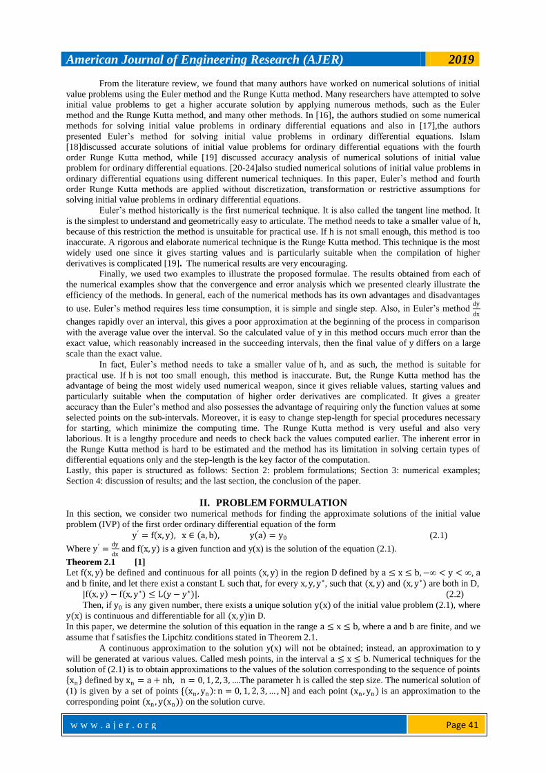
Figure 1: Exact Numerical Solution
Figure 2: Numerical Approximation for step size h=0.1
Figure 3: Numerical Approximation for step size h=0.05
0.00
2.00
4.00
6.00
8.00
10.00
12.00
14.00
16.00
18.00
0.00 0.10 0.20 0.30 0.40 0.50 0.60 0.70 0.80 0.90 1.00
Exact Solution
0.00
2.00
4.00
6.00
8.00
10.00
12.00
14.00
16.00
18.00
0.00 0.10 0.20 0.30 0.40 0.50 0.60 0.70 0.80 0.90 1.00
RK4 Approximation
Euler Approximation
0.00
2.00
4.00
6.00
8.00
10.00
12.00
14.00
16.00
18.00
0.00 0.10 0.20 0.30 0.40 0.50 0.60 0.70 0.80 0.90 1.00
RK4 Approximation
Euler Approximation

American Journal of Engineering Research (AJER) 2019
w w w . a j e r . o r g
w w w . a j e r . o r g
Page 48
Figure 4: Numerical Approximation for step size h=0.025
Figure 5: Numerical Approximation for step size h=0.0125
Figure 6: Error for different step size using RK4 method
0.00
2.00
4.00
6.00
8.00
10.00
12.00
14.00
16.00
18.00
0.00 0.10 0.20 0.30 0.40 0.50 0.60 0.70 0.80 0.90 1.00
RK4 Approximation
Euler Approximation
0.00
2.00
4.00
6.00
8.00
10.00
12.00
14.00
16.00
18.00
0.00 0.10 0.20 0.30 0.40 0.50 0.60 0.70 0.80 0.90 1.00
RK4 Approximation
Euler Approximation
0.000000
0.000050
0.000100
0.000150
0.000200
0.000250
0.000300
0.000350
0.000400
0.00 0.10 0.20 0.30 0.40 0.50 0.60 0.70 0.80 0.90 1.00
h=0.1
h=0.05
h=0.025
h=0.0125

American Journal of Engineering Research (AJER) 2019
w w w . a j e r . o r g
w w w . a j e r . o r g
Page 49
Figure 7: Error for different step size using Euler’s method
Example 2: We consider the initial value problem y′ = y − x2 + 1, y 0 = 0.5, on the interval0 ≤ x ≤ 2. The
exact solution of the given problem is given by y x = x2 + 2x + 1 − 0.5ex . The approximate results and the
absolute errors are obtained and shown in Tables 2(a)-(d) while the graphs of the numerical solutions are
displayed in Figures 8-14.
Table 2. (a) Numerical approximations and absolutes errors for step size h = 0.1; (b) Numerical approximations
and absolutes errors for step size h = 0.05; (c) Numerical approximations and absolutes errors for step size
h = 0.025, (d) Numerical approximations and absolutes errors for step size h = 0.0125.
(a) 𝐧 𝐱𝐧 Exact Solution
𝐲𝐧
Runge Kutta Method 𝐡 = 𝟎. 𝟏 Euler Method 𝐡 = 𝟎. 𝟏
𝐲 𝐱𝐧 𝐞𝐫𝐫𝐨𝐫𝐬 𝐲 𝐱𝐧 𝐞𝐫𝐫𝐨𝐫𝐬
0 0.0 0.5000000000 0.5000000000 0.0000000000 0.5000000000 0.0000000000
1 0.1 0.6574145401 0.6574143750 0.0000001660 0.6500000000 0.0074145410
2 0.2 0.8292986209 0.8292982760 0.0000003449 0.8140000000 0.0152986209
3 0.3 1.0150705962 1.0150700584 0.0000005378 0.9914000000 0.0236705962
4 0.4 1.2140876511 1.2140869057 0.0000007455 1.1815400000 0.0325476512
5 0.5 1.4256393646 1.4256383956 0.0000009690 1.3836940000 0.0419453646
6 0.6 1.6489405998 1.6489393904 0.0000012094 1.5970634000 0.0518771998
7 0.7 1.8831236463 1.8831221786 0.0000014677 1.8207697400 0.0623539063
8 0.8 2.1272295358 2.1272277907 0.0000017451 2.0538467140 0.0733828218
9 0.9 2.3801984444 2.3801964018 0.0000020426 2.2952313854 0.0849670590
10 1.0 2.6408590858 2.6408567242 0.0000023616 2.5437545239 0.0971045619
(b) 𝐧 𝐱𝐧 Exact Solution 𝐲𝐧 Runge Kutta Method 𝐡 = 𝟎. 𝟎𝟓 Euler Method 𝐡 = 𝟎. 𝟎𝟓
𝐲 𝐱𝐧 𝐞𝐫𝐫𝐨𝐫𝐬 𝐲 𝐱𝐧 𝐞𝐫𝐫𝐨𝐫𝐬
0 0.0 0.5000000000 0.5000000000 0.0000000000 0.5000000000 0.0000000000
1 0.1 0.6574145401 0.6574145304 0.0000000106 0.6536250000 0.0037895410
2 0.2 0.8292986209 0.8292985989 0.0000000220 0.8214715625 0.0078270584
3 0.3 1.0150705962 1.0150705619 0.0000000343 1.0029473977 0.0121231986
4 0.4 1.2140876511 1.2140876036 0.0000000475 1.1973995059 0.0166881453
5 0.5 1.4256393646 1.4256393029 0.0000000618 1.4041079553 0.0215314094
6 0.6 1.6489405998 1.6489405227 0.0000000771 1.6222790207 0.0266615791
7 0.7 1.8831236463 1.8831235527 0.0000000935 1.8510376203 0.0320860260
8 0.8 2.1272295358 2.1272294246 0.0000001111 2.0894189764 0.0378105594
9 0.9 2.3801984444 2.3801983144 0.0000001300 2.3363594215 0.0438390230
10 1.0 2.6408590858 2.6408589355 0.0000001503 2.5906862622 0.0501728236
(c)
n xn Exact Solution yn Runge Kutta Method h = 0.025 Euler Method h = 0.025
y xn 𝐞𝐫𝐫𝐨𝐫𝐬 y xn 𝐞𝐫𝐫𝐨𝐫𝐬
0 0.0 0.5000000000 0.5000000000 0.0000000000 0.5000000000 0.0000000000
1 0.1 0.6574145401 0.6574145403 0.0000000007 0.6554982324 0.0019163085
2 0.2 0.8292986209 0.8292986195 0.0000000014 0.8253384788 0.0039601421
3 0.3 1.0150705962 1.0150705940 0.0000000022 1.0089333673 0.0061372289
0.000000
0.500000
1.000000
1.500000
2.000000
2.500000
3.000000
0.00 0.10 0.20 0.30 0.40 0.50 0.60 0.70 0.80 0.90 1.00
h=0.1
h=0.05
h=0.025
h=0.0125

American Journal of Engineering Research (AJER) 2019
w w w . a j e r . o r g
w w w . a j e r . o r g
Page 50
4 0.4 1.2140876511 1.2140876482 0.0000000030 1.2056345492 0.0084531020
5 0.5 1.4256393646 1.4256393608 0.0000000039 1.4147263688 0.0109129958
6 0.6 1.6489405998 1.6489405949 0.0000000049 1.6354188765 0.0135217233
7 0.7 1.8831236463 1.8831236404 0.0000000059 1.8668401152 0.0162835311
8 0.8 2.1272295358 2.1272295287 0.0000000070 2.1080276077 0.0192019281
9 0.9 2.3801984444 2.3801984362 0.0000000082 2.3579189592 0.0222794852
10 1.0 2.6408590858 2.6408590763 0.0000000095 2.6153414848 0.0255176010
(d) n xn Exact Solution yn Runge Kutta Method h = 0.0125 Euler Method h = 0.025
y xn 𝐞𝐫𝐫𝐨𝐫𝐬 y xn 𝐞𝐫𝐫𝐨𝐫𝐬
0 0.0 0.5000000000 0.5000000000 0.0000000000 0.5000000000 0.0000000000
1 0.1 0.6574145401 0.6574145409 0.0000000000 0.6564508731 0.0009636678
2 0.2 0.8292986209 0.8292986208 0.0000000001 0.8273066068 0.0019920141
3 0.3 1.0150705962 1.0150705961 0.0000000001 1.0119825867 0.0030880095
4 0.4 1.2140876511 1.2140876510 0.0000000002 1.2098331143 0.0042545368
5 0.5 1.4256393646 1.4256393644 0.0000000002 1.4201450250 0.0054943397
6 0.6 1.6489405998 1.6489405995 0.0000000003 1.6421306378 0.0068099620
7 0.7 1.8831236463 1.8831236459 0.0000000004 1.8749199705 0.0082036758
8 0.8 2.1272295358 2.1272295353 0.0000000004 2.1175521396 0.0096773962
9 0.9 2.3801984444 2.3801984439 0.0000000005 2.3689658626 0.0112325818
10 1.0 2.6408590858 2.6408590852 0.0000000006 2.6279889679 0.0128701179
Figure 8: Exact Numerical Solution
Figure 9: Numerical Approximation for step size h=0.1
0.00
0.50
1.00
1.50
2.00
2.50
3.00
0.00 0.10 0.20 0.30 0.40 0.50 0.60 0.70 0.80 0.90 1.00
Exact Solution
0.00
0.50
1.00
1.50
2.00
2.50
3.00
0.00 0.10 0.20 0.30 0.40 0.50 0.60 0.70 0.80 0.90 1.00
RK4 Approximation
Euler Approximation
American Journal of Engineering Research (AJER) 2019
w w w . a j e r . o r g
w w w . a j e r . o r g
Page 51
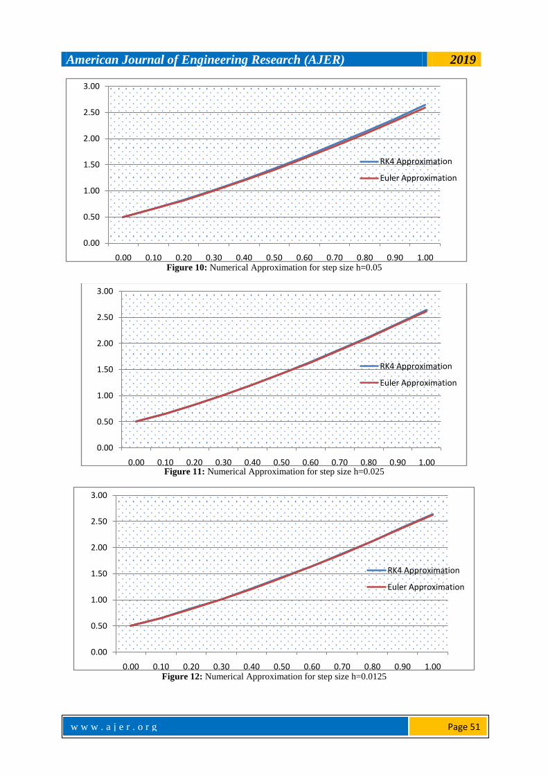
Figure 10: Numerical Approximation for step size h=0.05
Figure 11: Numerical Approximation for step size h=0.025
Figure 12: Numerical Approximation for step size h=0.0125
0.00
0.50
1.00
1.50
2.00
2.50
3.00
0.00 0.10 0.20 0.30 0.40 0.50 0.60 0.70 0.80 0.90 1.00
RK4 Approximation
Euler Approximation
0.00
0.50
1.00
1.50
2.00
2.50
3.00
0.00 0.10 0.20 0.30 0.40 0.50 0.60 0.70 0.80 0.90 1.00
RK4 Approximation
Euler Approximation
0.00
0.50
1.00
1.50
2.00
2.50
3.00
0.00 0.10 0.20 0.30 0.40 0.50 0.60 0.70 0.80 0.90 1.00
RK4 Approximation
Euler Approximation

American Journal of Engineering Research (AJER) 2019
w w w . a j e r . o r g
w w w . a j e r . o r g
Page 52
Figure 13: Error for different step size using RK4 method
Figure 14: Error for different step size using Euler’s method
IV. DISCUSSION AND RESULTS The obtained results are displayed in Table 1(a)-(d) and Table 2(a)-(c) and graphically represented in
Figures (1-7) and Figures (8-14) respectively. The approximate solutions and absolute errors are calculated
using Matlab programming language with the step sizes 0.1, 0.05, 0.025, and 0.0125 and also computed with
the exact solution. From the tables for each of the methods, we observed that the numerical solutions converge
to the exact solution and the errors incurred in the Euler’s method are greater than that of the Runge Kutta
method. We also observed that the Runge Kutta approximations for the same size converge firstly to the exact
solution. This indicates that the small step size provides a better approximation. The fourth order Runge Kutta
method is laborious, it requires four evaluations per step size, but it gives more accurate results than the Euler’s
method with only one-fourth the step size. We equally observed that the fourth order Runge Kutta Method
converges faster, more accurate and cost effective than the Euler’s method (as can be seen in the tables and
figures) in solving initial value problems in ordinary differential equations.
V. CONCLUSION In this paper, the fourth order Runge Kutta and Euler’s methods are used for solving initial value
problems (IVP) in Ordinary Differential Equations (ODE). To find more accurate results, we reduced the step
size for both methods. From our tables and figures, we analyzed that the solution for both methods converges to
the exact solution for decreasing the step size h. The numerical solutions obtained by the two methods are in
good agreement with the exact solutions. However, by comparing the results of the two methods, we state that
the RK4 Method is appropriate, consistent, convergent, quite stable, and more accurate than the Euler’s method
and it is widely used in numerical solutions of initial value problems in ordinary differential equations. In our
0.000000
0.000001
0.000001
0.000002
0.000002
0.000003
0.00 0.10 0.20 0.30 0.40 0.50 0.60 0.70 0.80 0.90 1.00
h=0.1
h=0.05
h=0.025
h=0.0125
0.000000
0.020000
0.040000
0.060000
0.080000
0.100000
0.120000
0.00 0.10 0.20 0.30 0.40 0.50 0.60 0.70 0.80 0.90 1.00
h=0.1
h=0.05
h=0.025
h=0.0125

American Journal of Engineering Research (AJER) 2019
w w w . a j e r . o r g
w w w . a j e r . o r g
Page 53
subsequent research, we shall examine the comparison of RK4 method with other existing method like the
Adomian decomposition.
REFERENCES [1]. Lambert,J. (2000). Computational Methods in Ordinary Differential Equations. New York: Wiley & Sons: 21-205IEA: [2]. Butcher ,J. (2003).Numerical Methods for Ordinary Differential Equations. West Sussex: John Wiley & Sons Ltd. 45-95.
[3]. Atkinson K, Han W, Stewart D, (2009) Numerical Solution of Ordinary Differential Equations. New Jersey: John Wiley & Sons,
Hoboken: 70-87. [4]. Euler L, (1768) Institutiones Calculi IntegralisVolumenPrimum, Opera Omnia. Vol. XI, B. G. TeubneriLipsiaeetBerolini
MCMXIII: 21-228.
[5]. Euler, L. (1913).De integration aequationum di erentialium per approximationem, In Opera Omnia, 1st series, Vol II, Institutiones Calculi Integralis, Teubner, Leipzig and Berlin, 424434.
[6]. Brenan, K., Campbell S, Petzold L, (1989).Numerical Solution of Initial-Value Problems in Differential-Algebraic Equations. New
York: Society for Industrial and Applied Mathematics: 76-127. [7]. Lambert, J. (1999).Numerical Methods for Ordinary Differential Systems: The Initial value Problem. New York: John Wiley
&Sons: 149-205.
[8]. Boyce W, DiPrima R, (2000) Elementary Differential Equations and Boundary Value Problems. New York: John Wiley & Sons, Inc.: 419-471.
[9]. Carnahan, B,, Luther, H., Wikes, J. (1990). Applied Numerical Methods, Florida: Krieger Publishing Company: 341-386.
[10]. Chapra, S.,Canale, R. (2006). Applied Numerical Methods with MATLAB for Engineers and Scientists, 6 Ed,. Boston: McGraw
Hill: 707-742.
[11]. Esfandiari R, (2013) Numerical Methods for Engineers and Scientists using MATLAB. New York: CRC Press (CRC), Taylor & Francis Group: 329-351.
[12]. Fatunla, S., (1988).Numerical Methods for Initial Value Problems in Ordinary Differential equations. Boston: Academic Press,
INC: 41-62. [13]. Conte, S., Boor,C.Elementary Numerical Analysis: Algorithmic Approach. New York: McGraw-Hill Book Company: 356-387.
[14]. Kreyszig, E. (2011).Advanced Engineering Mathematics, 10 Eds,. Boston: John Wiley & Sons, Inc: 921-937.
[15]. Iserles, A. (1996).A First Course in the Numerical Analysis of Differential Equations, Cambridge: Cambridge University Press: 1-50.
[16]. Bosede, O., Emmanuel, F.,Temitayo, O. (2012). On Some Numerical Methods for Solving Initial Value Problems in Ordinary
Differential Equations. IOSR Journal of Mathematics (IOSRJM) Vol. 1 (3): 25-31. [17]. Fadugba, S.,Ogunrinde, B., Okunlola, T. (2012).Euler’s Method for Solving Initial Value Problems in Ordinary Differential
Equations. The Pacific Journal of Science and Technology, Vol. 13 (2): 152-158.
[18]. Islam, Md. A. (2015). Accurate Solutions of Initial Value Problems for Ordinary Differential Equations with the Fourth Order Runge Kutta Method. Journal of Mathematics Research, Vol. 7 (3): 41-45.
[19]. Islam, M. A. (2015). Accurate Analysis of Numerical Solutions of Initial Value Problems (IVP) for ordinary differential equations
(ODE). IOSR Journal of Mathematics (IOSR-JM), Vol. 11 (3): 18-23. [20]. Jamali N, (2019) Analysis and Comparative Study of Numerical Methods to Solve Ordinary Differential Equation with Initial Value
Problem. International Journal of Advanced Research (IJAR). Vol. 7(5): 117-128: Available from:
http://www.journalijar.com/uploads/536_IJAR-27303.pdf. [21]. Hossain, B. B.,Hossain, M. J., MiahMd, et al. (2017) A Comparative Study on Fourth Order and Butcher’s Fifth Order Runge Kutta
Methods with Third Order Initial Value Problem (IVP). Applied and Computational Mathematics, Vol. 6(6): 243-253. Available
from: doi:10.11648/j.acm.20170606.12. [22]. Fadugba, S.E.,Olaosebikan, T.E, (2018). Comparative Study of a Class of One-Step Methods for the Numerical Solutions of Some
Initial Value Problems in ordinary Differential Equations. Research Journal of Mathematics and Computer Science: 2-9: Available
from: https://escipub.com/Articles/RJMCS/RJMCS-2017-12-1801. [23]. Hamed, A. B., Alrhaman, I. Y.,Sani, I, (2017). The accuracy of Euler and modified Euler technique for First Order Ordinary
Differential Equations with initial conditions. American journal of Engineering Research (AJER), Vol. 6(9): 334-338.
[24]. Oshinubi IK, Ogunjimi OA, Longe OB, (2017) On some Computational Methods for Solving an Ordinary Differential Equations with Initial Condition. Proceedings of the ISTEAMS Multidisciplinary Cross-Border Conference, University of Ghana, Legon: 73-
80.
Anthony Anya Okeke" Analysis and Comparative Study of Numerical Solutions of Initial
Value Problems (IVP) in Ordinary Differential Equations (ODE) With Euler and Runge Kutta
Methods"American Journal of Engineering Research (AJER), vol. 8, no. 8, 2019, pp. 40-53


![Comparative numerical evaluation for the low velocity ...carbonlett.org/Upload/files/CARBONLETT/[089-095]-09.pdf · 89 Comparative numerical evaluation for the low velocity impact](https://img.pdfslide.us/doc/110x75/5b5207767f8b9a56588cdd53/comparative-numerical-evaluation-for-the-low-velocity-089-095-09pdf-89.jpg)