Embed Size (px)
Citation preview
Analysis and clustering of residential customers energy behavioral demand using smart meter data Article
Accepted Version
Haben, S., Singleton, C. and Grindrod, P. (2016) Analysis and clustering of residential customers energy behavioral demand using smart meter data. IEEE Transactions on Smart Grid, 7 (1). pp. 136144. ISSN 19493053 doi: https://doi.org/10.1109/TSG.2015.2409786 Available at http://centaur.reading.ac.uk/47589/
It is advisable to refer to the publisher’s version if you intend to cite from the work. Published version at: http://ieeexplore.ieee.org/xpl/articleDetails.jsp?arnumber=7063233
To link to this article DOI: http://dx.doi.org/10.1109/TSG.2015.2409786
Publisher: IEEE
All outputs in CentAUR are protected by Intellectual Property Rights law, including copyright law. Copyright and IPR is retained by the creators or other copyright holders. Terms and conditions for use of this material are defined in the End User Agreement .
www.reading.ac.uk/centaur

CentAUR
Central Archive at the University of Reading
Reading’s research outputs online

Analysis and Clustering of Residential
Customers Energy Behavioral Demand Using
Smart Meter Data
Stephen Haben*, Colin Singleton**, and Peter Grindrod*
*Mathematical Institute, University of Oxford, Oxford, OX2 6GG,
UK, e-mail: [email protected]**CountingLab Limited, Reading, RG6 6AX, UK, email:
November 27, 2015
Abstract
Clustering methods are increasingly being applied to residential smartmeter data, providing a number of important opportunities for distri-bution network operators (DNOs) to manage and plan the low voltagenetworks. Clustering has a number of potential advantages for DNOsincluding, identifying suitable candidates for demand response and im-proving energy pro�le modelling. However, due to the high stochasticityand irregularity of household level demand, detailed analytics are requiredto de�ne appropriate attributes to cluster. In this paper we present in-depth analysis of customer smart meter data to better understand peakdemand and major sources of variability in their behaviour. We �nd fourkey time periods in which the data should be analysed and use this toform relevant attributes for our clustering. We present a �nite mixturemodel based clustering where we discover 10 distinct behaviour groups de-scribing customers based on their demand and their variability. Finally,using an existing bootstrapping technique we show that the clusteringis reliable. To the authors knowledge this is the �rst time in the powersystems literature that the sample robustness of the clustering has beentested.
1 Introduction
In power systems, clustering methods have traditionally been applied to energydata of high/medium voltage customers or on larger aggregations of customers[8], [7]. In recent years, research has increasingly considered clustering at thehousehold level based on half hourly energy demand recorded by smart meters
1

[14]. Such methods are driven by the need for energy suppliers and distributionnetworks operators (DNOs) to better understand how residential customers usetheir energy and their e�ect on the low voltage (LV) networks. This issue isincreasingly relevant as energy demand changes dramatically with the uptakeof new technologies such as electric vehicles, photovoltaics, combined heat andpower. In addition, new large energy demand technologies, not even thoughtof, could also be introduced, as shown by virtual currency mining. The UKroll-out of smart meters is expected to be complete by 2020 and will providegreater visibility of all residential customers energy use. However, since suchdata is proprietary it is not certain if DNOs will have complete access to suchdata and, even if it can be purchased, it is likely to be expensive [12]. Hencethe value of the data must be properly assessed before infrastructure is put inplace to manage it.
Smart meter data is being analysed through publicly available data sets suchas the Irish smart meter trial and other research projects [5], [16], [17]. Cluster-ing customers based on attributes derived from smart meter data creates betterunderstanding of the di�erent types of energy behavioral groups. The focus ofthis paper is to derive and cluster suitable attributes from smart meter datawhich can assist a DNO with two main applications for better LV network mod-eling and management. The primary application that motivates our approachis to help a DNO identify suitable customers for energy management solutionssuch as demand side response (DSR) and through storage devices. These ap-plications have already been considered recently by a number of authors, seefor example [5], [18], [10]. By choosing the correct attributes a DNO can usethe clustering to identify suitable customer groups for demand reduction solu-tions and hence help to reduce network demand and volatility. For example,customers with heavy but regular demand in the evening time period could beideal candidates for peak demand reduction through storage devices, whereasthose with irregular demand may be more suitable for DSR. The secondaryapplication is for identifying links between energy behavioural usage and pub-licaly available information (such as house-type and socio-demographics) [15],[3]. Such links can be used to improve modeling of residential customer demandand reduce necessary monitoring on the LV network. However, besides thesetwo, the methodology can also be used for further applications of smart meterbased clustering which we present in Section 2.
Choosing the correct attributes is potentially the most important aspectof a successful clustering. This is particularly challenging when consideringextremely volatile household level demand which is much less regular than highervoltage demands [16]. The number of attributes should be optimized to: ensurethe data distribution over parameter space is dense, reduce computational costs,and ensure the results can be easily interpreted [23]. In addition, if the numberof attributes is not optimized then the clustering is less likely to be representativeand �t for purpose. A main contribution of this paper is a detailed analysis ofa large amount of domestic smart meter data, especially with regard to betterunderstanding of peak demands and sources of variability. This helps us toidentify and minimise the important attributes to be used in the clustering.
2
In addition, we discover four key time periods within which data should beanalysed since they describe the most frequent largest demand behaviour.
There have been a variety of clustering methods which have been applied inthe power systems literature [7], [3], [24]. In this paper we cluster our attributesby considering it as a �nite mixture model (FMM) of Gaussian multivariatedistributions, we justify the choice of method in Section 3 [19]. FMM are rarelyapplied to cluster smart meter data despite their versatility compared to themore common k-means method. We check the reliability of the outputs of theFMM clustering using a bootstrapping technique [13]. To the authors knowl-edge, checks of clustering reliability in the power systems literature have notbeen considered. We follow the bootstrapping method as described in [11].Checking the sample robustness of the clustering is a vital part of ensuring thatthe �nal clustering is robust with respect to the sample used. This work hasbeen developed in collaboration with Scottish and Southern energy power dis-tribution, one of the DNOs in the UK, as part of the New Thames Valley Vision(NTVV) project.
In section 2 we perform a literature review of the recent clustering beingapplied to household level energy demand. In section 3 we introduce the theorybehind the �nite mixture model and the bootstrapping method for our �nalclustering. We derive the attributes selection in section 4 and apply the clus-tering and bootstrapping in section 5. In section 6 we summarise the paper andoutline future work.
2 Literature Review
Historically, electricity data for a household is only available from real or esti-mated quarterly cumulatives which reveal no intraday information of a house-holds electric usage behaviour. As such, much research has tried to infer en-ergy demand characteristics from other sources such as socio-demographics andhousehold properties (house type, size etc.). Although there exist correlationsbetween some characteristics and attributes, such as maximum demand, theyare weak and do not describe intra-day behaviours [20], [26, p.74]. There arealso several studies which show there is a large degree of variation in demandswhich cannot be accounted for despite similar dwelling types, size and occu-pants (see [21] and references therein.). Other work has also shown that thereare poor links between energy behaviour and typical socio-demographic classi�-cations [15]. This suggests that to understand customer energy usage behaviourrequires analysing actual consumption data.
Clustering at the individual domestic customer level has many potential usesfor energy companies. In particular, clustering can ensure that experiments in-clude a representative sample of the population (by requiring a su�cient numberof customers in each group); allows an experimenter to adjust results to re�ectbiases in their sample; identify which characteristics correlate with energy be-havioral use [3], [20]; help create more suitable tari�s [14]; and more accuratecustomer pro�les [23], [25]; identify which customers are viable for energy saving
3
solutions such as demand response [5], [2], [10], [18]; identify which combinationof customer types can cause network constraint violations; improving forecastmethodologies [22], [6]; and compare di�erent groups and trends in behaviour.
There are a large number of clustering methods which have been appliedto household level data including, k-means and k-mediods [14], [23], [10], [4],�nite mixture models [24], [25], principle component analysis, [1], self organizingmaps [3] and spectral clustering [2]. Perhaps more important than the methodsused in the clustering is the attributes which are clustered. These split intotwo main categories, those which try to cluster the full time series (for example48 half hours a day) [14] and those which cluster speci�c features such as sizeof peak demand or distribution parameters [23], [10]. It is often preferable tocluster as few attributes as possible since this reduces computational expenseand makes the clustering less sensitive to missing values [23]. This also avoidsthe curse of dimensionality. For example, if clustering hourly data over a day,and assuming a simple case where each hour can only take two values, a high andlow, then there are potentially 224 ≈ 16.8m di�erent time series, which requiresa huge number of clusters to isolate the distinct behaviours. Similarly, choosinga reduced number of features requires that they describe as much information aspossible to be useful. This is particularly challenging for the volatile residentialdemand usage where a large number of behaviours can potentially exist.
3 Finite Mixture Modelling
Finite mixture models (FMMs) are a commonly used technique in clusteringdata attributes and have recently been used in clustering smart meter data [19],[25]. There are a number of practical advantages for clustering using FMMswhich we discuss in this Section. A main advantage of FMMs over many othernon-hierarchical clustering methods, such as k-means, is the ability to modela mixture of both continuous and categorical data. Categorical data can beparticularly useful for including identi�ers of low carbon technologies, for exam-ple electric vehicles which, although not implemented in this research, may bedesirable in future clusterings. The FMM is set in a statistical framework anddescribes the distributions and correlations between attributes by automaticallychoosing the optimal weights for each of the input parameters for each cluster.This is in contrast to the k-means which is essentially a FMM but where theweights (axis scales) are �xed a priori. Additionally for FMMs there is no needto pre-de�ne a distance measure and it allows variability for each attribute ona cluster-by-cluster level. A �nal advantage of the method is that the Bayesianinformation criterion (BIC), a common statistical criterion for selecting the op-timal number of clusters, can be calculated as a by-product of the likelihoodframework of the FMM for no extra cost. Disadvantages of the FMMs are thatthe number of clusters must be chosen a priori, the algorithm can converge tolocal optima and the method is sensitive to the input attributes chosen. Giventhe pros and cons, FMMs seem a suitable choice for our clustering task.
We describe the main properties of FMMs in this Section, for further details
4
see [19]. In FMMs we assume measurements are described by a �nite mixtureof distributions, typically from a single parametric family. The problem is oftenaddressed using the expectation-maximization (EM) algorithm which considersthe so-called incomplete problem [19]. In this setting the observed data is mod-elled as incomplete since information on which cluster an observations belongsto is unknown. A log likelihood function is formed which must be maximizedto �nd the correct mixing proportions and parameters for the distributions.
The EM algorithm iteratively �nd a local maximum of the system by alter-nating between an E-step and M-step. In the E-step we calculate the expectedlog-likelihood, given the current values, to update the posterior probabilitiesof the component label vectors, where the probability of the jth observationbeing in the ith cluster is denoted by τi,j . In the M-step, using the posteriorprobabilities, the expected log-likelihood function is maximized to update themixing proportions and the distribution parameters. Once convergence has beenachieved a soft or hard clustering can be produced. In the soft clustering eachobservation is assigned to every cluster with a certain probability determinedby the �nal posterior probabilities, τi,j , of the component labels. In the hardclustering the observation is assigned to the cluster with the largest posteriorprobability. In this paper we assume the underlying distributions are inde-pendent Gaussians, this has the added advantage that the E and M steps areparticularly easy to calculate [19]. Caution must be displayed when implement-ing the EM algorithm. The EM algorithm converges quickly, but not necessarilyto a global maximum, thus the algorithm must be run repeatedly, with di�erentinitial conditions, to ensure global convergence is achieved.
In non-hierarchical clustering there is always an ambiguity choosing the op-timal number of clusters. A compromise must be made between having su�-ciently many clusters to describe the majority of the variability, but few enoughto avoid large dimensionality and ensure they are manageable. There are manyclustering performance measures that have been developed [9]. For our work weconsider the Bayesian information criterion (BIC) due to its statistical relevanceand its ease of calculation within the log-likelihood framework of the FMM [19].Essentially, the BIC penalizes the likelihood in proportion to the number ofparameters in the model. An alternative to the BIC is the Akaike informationcriterion but we choose the BIC as it penalizes the number of parameters morestrongly and, for operational reasons, we do not want too many clusters. Ob-serving how the BIC improves as we increase the number of clusters allows usto justify the appropriate number of groups to use in the �nal clustering.
3.1 Bootstrapping
After producing the �nal clusters, the natural question arises as to how reliableare the outputs? This has not been considered in the clustering methods inthe powers systems literature but is important for testing the robustness of theresults. A reliable segmentation means that, for any individual household, weare quite certain which cluster the household belongs to. There are numerousreasons why a clustering might be unreliable. The technique used might be poor
5

(inappropriate for the data); the wrong attributes may be chosen; the nature ofthe data one is using might not lend itself to clustering; or there just might notbe enough data for the clustering to be reliable.
Bootstrapping methods are common tests for measuring the accuracy ofparameter estimates (for example, the variance or mean) of the underlying,unknown, true distribution, by sampling from an approximate distribution [13].Bootstrapping is particularly useful when there is a small amount of empiricaldata, as in our case with only 3622meters available. Traditionally bootstrappingis repeated hundreds or thousands of times for various alternative realizationsof the data. Thus one covers a large number of the possibilities that couldhave occurred (although the number of possibilities is extremely large), enoughto estimate uncertainties around the measurements and statistics of interest.The reliability of the bootstrap method depends upon the number of timesthe process is repeated (which we are free to choose) and also how well theunderlying distribution can be approximated from the real data. We note thatthis method is dissimilar to cross-validation methods which serve to validate themodel rather than estimating the uncertainty of our classi�cation.
For our clustering we resample, with replacement, the attributes from N =3622 customers from the data and then recluster, we repeat this M = 10, 000times. Following the work in [11] we calculate particular variables to indicatethe robustness of our clustering. We �rst consider a measure of classi�cationuncertainty for customer j given by
ej = mini(1− τi,j), (1)
where τi,j are the �nal posterior probabilities found for the current bootstrap.The classi�cation uncertainty is the sum of the probabilities of all the classesthat customer j does not belong. If classi�cation is certain ej is close to zero. Ifuncertain then ej will be close to (g−1)/g, (i.e. random) where g is the numberof groups in the clustering. We keep track of ej for each customer for eachbootstrap. As an aggregate measure of the uncertainty of the overall clustermodel we consider
E = 1− EN(τ)/(N log(g)), (2)
where
EN(τ) = −N∑j=1
g∑k=1
τk,j log(τk,j). (3)
The relative entropy, E, provides an estimate as to how well separated theclasses are, with E close to one for well separated classes and E close to zerofor poorly separated classes. We can obtain an estimate of E from the originaldata with the EM-algorithm but the bootstrap can also be used to provide anestimate of how robust the clustering is to sampling errors.
Finally we consider the mean and variance of each parameter within eachclass. In an ideal situation these values will be the very similar in each bootstrapbut due to errors through relabelling we simply use the means (ignoring thevariances) and for each parameter, report the nearest class mean value to the
6
one obtained with the true (original) sample. This may underestimate theuncertainty in the mean parameter value for that class but at least should givesome indication. We then average over all these "nearest means" to obtain arough estimate of the sampling uncertainty in the de�nition of the cluster mean.
4 Data Analysis and Attribute Selection
Choosing the appropriate attributes for the application is essential if we areto produce informative groups from our clustering. Our main application is toidentify households who are appropriate for demand reduction through demandside response or the implementation of storage devices. Hence, we are interestedin discovering clusters describing the di�erent types of peak demands and majorvariabilities and seasonalities in the data. In order to reduce the dimensionality,in this work we focus on clustering on a limited number of attributes. Wediscover four key time periods in which the data should be analysed. Thisenables us to choose a lower temporal resolution version of the smart meterdata to best describe customer peak demand behaviour.
The data used in the clustering is from the publicly available Irish smartmeter trial which consists of half hourly energy readings from smart meter datafor just under 4000 residential customers from around Ireland [17]. We consid-ered the �rst year of data (starting midnight 14th July 2009) and after removingcustomers with spurious and missing data reduced the set to 3622 customers. Inthe trial the customers are assigned to di�erent tari�s but we do not distinguishthem in the clustering we present in Section 5. Fig. 1 shows the normalizedvariation of the half hourly demand against the mean for each customer. The�gure highlights two important features which must be considered before we cre-ate our attributes. Firstly the variability in the mean daily demands indicatesthat it is important to normalise features which describe the intra-day demandsince otherwise the �nal clusters may simply describe the mean demand and notthe distribution of demand over the day [7], [14]. Secondly the wide spread innormalized standard deviation shows the importance, when describing averageattributes, to include a measure of the variability to get a fuller understandingof the customer behavioral use. Without such a measure we have a limitedunderstanding of how representative the mean cluster value is of its members.
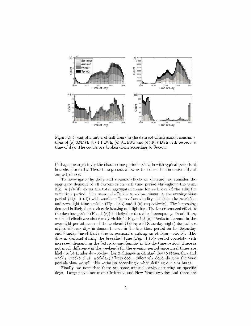
Due to the natural volatility of residential customers, modelling peak demandis challenging. For most customers (2700) a large peak usage of 5kWh over anyhalf hour, occurs at least once throughout the year but these occur less than 5%of all half hours in the dataset. A much more managable, but still important,task is to understand the occurance of frequently occuring daily peak demands.Fig. 2 shows a count according to time of day of when di�erent size peaks occur.The counts are broken down according to seasons (seasons are determined bystandard equinox and solstice dates for Ireland) and show that di�erent sizepeaks occur at di�erent times of the day depending on the season.
The plots show consistent time intervals during the day when the largest de-mands occur. In addition, the largest demands are quite seasonally driven and
7

0 0.5 1 1.5 2 2.50
0.2
0.4
0.6
0.8
1
1.2
1.4
1.6
1.8
2
Mean Daily Usage (kWh)
Nor
mal
ised
Sta
ndar
d D
evia
tion
Figure 1: Normalized standard deviation of daily demand versus mean dailydemand for each residential customer.
occur at particular time intervals. For example, in Fig. 2 (a) and (b), when con-sidering smaller demands, the distributions are focused during the evening timeperiod (about 3.30pm to 10.30pm) and also the daytime (about 9am-3.30pm).In addition, the daytime peaks are weighted towards weekend days (not shown)as expected. In contrast, the largest peaks, as shown by Fig. 2 (c) and (d), showthat the breakfast time period (about 6.30am-9am) and overnight time period(about 10.30pm to 6.30am) become more prominent. In particular the overnighttime period is likely to be due to high energy overnight storage heaters whichcoincides with the fact that the majority of these peaks are from the Autumnand Winter seasons. However, we note that the the largest demands, as shownin Fig. 2 (d) consists of, circa 1000 individual customer half hours, which is arelatively small fraction of the 63m customer-half-hours considered and smallcompared with the number of customer-half hours exceeding 0.9kWh as shownin Fig. 2 (a) which is of an order of magnitude of around 105.
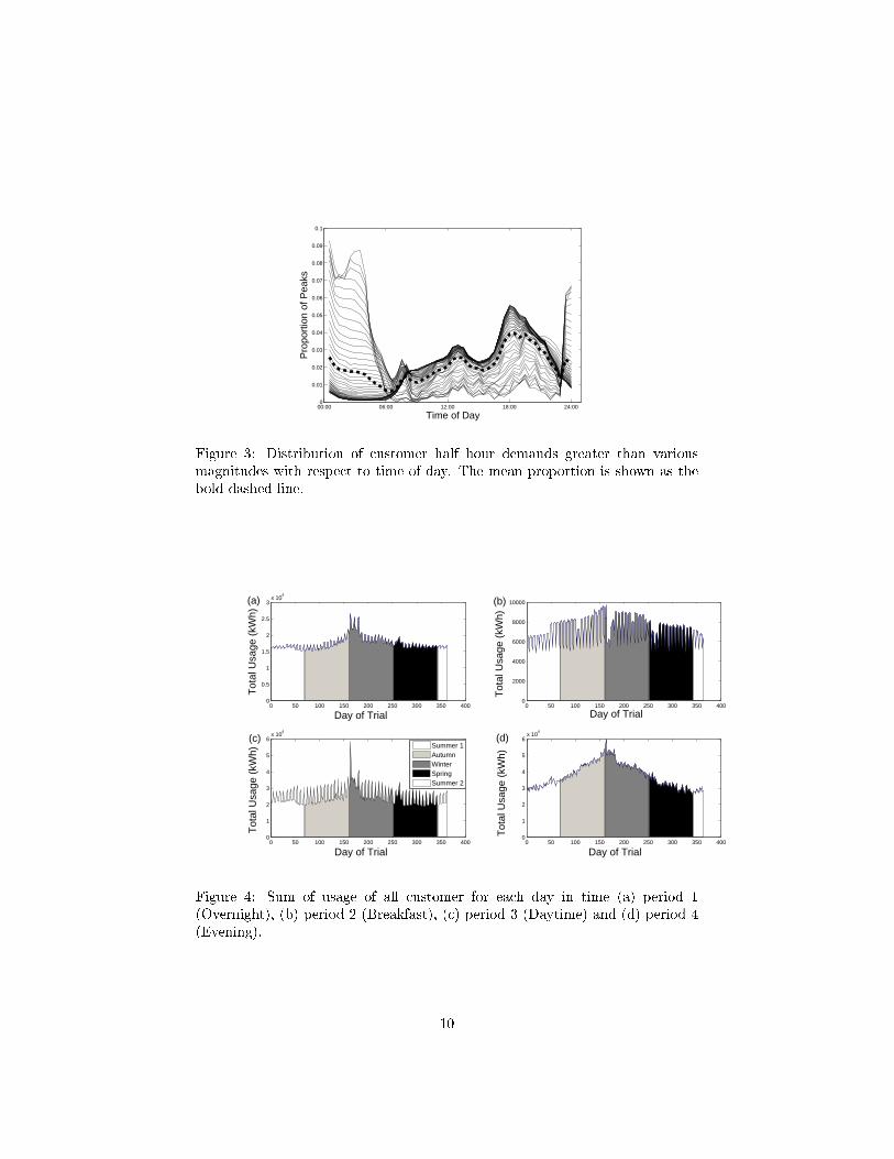
Fig. 3 shows the distribution of peaks for a larger number of demands from0.9kWh to 11kWh in 0.2 kWh intervals. The plot con�rms Fig. 2 with thelargest distributions of peak demand occurring in four time periods as indicatedby the four local maxima in the distributions. The mean proportion is shownfor clarity and again indicates that there are some common time periods wherelarger demands tend to occur. Motivated by this analysis we de�ne four keytime periods, chosen by the approximate local minimums between the modalpeak times as shown in Fig. 3. The four chosen time periods are
• Time period 1: 10.30pm-6.30am - The Overnight period
• Time period 2: 6.30am-9.00am - The Breakfast period
• Time period 3: 9.00am-3.30pm - The Daytime period
• Time period 4: 3.30pm-10.30pm - The Evening period
8
00:00 06:00 12:00 18:00 24:000
1
2
3
4
5x 10
5
Time of Day
Cou
nt
SummerAutumnWinterSpring
00:00 06:00 12:00 18:00 24:000
2000
4000
6000
8000
10000
12000
14000
16000
Time of Day
Cou
nt
00:00 06:00 12:00 18:00 24:000
50
100
150
200
250
300
Time of Day
Cou
nt
00:00 06:00 12:00 18:00 24:000
20
40
60
80
100
120
Time of Day
Cou
nt
(b)(a)
(c) (d)
Figure 2: Count of number of half hours in the data set which exceed consump-tions of (a) 0.9kWh (b) 4.1 kWh, (c) 8.1 kWh and (d) 10.7 kWh with respect totime of day. The counts are broken down according to Season.
Perhaps unsurprisingly the chosen time periods coincide with typical periods ofhousehold activity. These time periods allow us to reduce the dimensionality ofour attributes.
To investigate the daily and seasonal e�ects on demand, we consider theaggregate demand of all customers in each time period throughout the year.Fig. 4 (a)-(d) shows the total aggregated usage for each day of the trial foreach time period. The seasonal e�ect is most prominent in the evening timeperiod (Fig. 4 (d)) with smaller e�ects of seasonality visible in the breakfastand overnight time periods (Fig. 4 (b) and 4 (a) respectively). The increasingdemand is likely due to electric heating and lighting. The lower seasonal e�ect inthe daytime period (Fig. 4 (c)) is likely due to reduced occupancy. In addition,weekend e�ects are also clearly visible in Fig. 4 (a)-(c). Peaks in demand in theovernight period occur at the weekend (Friday and Saturday night) due to latenights whereas dips in demand occur in the breakfast period on the Saturdayand Sunday (most likely due to occupants waking up at later periods). Thedips in demand during the breakfast time (Fig. 4 (b)) period correlate withincreased demand on the Saturday and Sunday in the daytime period. There isnot much di�erence in the weekends for the evening period since meal times arelikely to be similar day-to-day. Large changes in demand due to seasonality andweekly (weekend vs. weekday) e�ects occur di�erently depending on the timeperiods thus we split this variation accordingly when de�ning our attributes.
Finally, we note that there are some unusual peaks occurring on speci�cdays. Large peaks occur on Christmas and New Years eve/day and there are
9
00:00 06:00 12:00 18:00 24:000
0.01
0.02
0.03
0.04
0.05
0.06
0.07
0.08
0.09
0.1
Time of Day
Pro
port
ion
of P
eaks
Figure 3: Distribution of customer half hour demands greater than variousmagnitudes with respect to time of day. The mean proportion is shown as thebold dashed line.
0 50 100 150 200 250 300 350 4000
0.5
1
1.5
2
2.5
3x 10
4
Tot
al U
sage
(kW
h)
0 50 100 150 200 250 300 350 4000
2000
4000
6000
8000
10000
Tot
al U
sage
(kW
h)
0 50 100 150 200 250 300 350 4000
1
2
3
4
5
6x 10
4
Tot
al U
sage
(kW
h)
0 50 100 150 200 250 300 350 4000
1
2
3
4
5
6x 10
4
Tot
al U
sage
(kW
h)
Summer 1AutumnWinterSpringSummer 2
Day of Trial
(a) (b)
(d)(c)
Day of Trial
Day of Trial
Day of Trial
Figure 4: Sum of usage of all customer for each day in time (a) period 1(Overnight), (b) period 2 (Breakfast), (c) period 3 (Daytime) and (d) period 4(Evening).
10

increases in demand during the Easter holidays (4th April 2010). There is aparticularly large demand on the 9th and 10th of January 2010. This could berelated to the extreme Winter weather conditions which occurred on this day1.The special days: Christmas eve and day, New years eve and day and the 9/10January are removed from our analysis to ensure that we are modelling thetypical behaviour of customers. Such days would be perhaps better modelledon a case-by-case basis. There is also variability which may not be accountedfor by the seasonality and type of day. For this reason we also must include ageneral measure of the variability and irregularity of each customer.
To de�ne our attributes we introduce some notation. For a particular cus-tomer we de�ne Pi to be the mean power in each time period i = 1, 2, 3, 4 overthe entire years worth of data, with corresponding standard deviation σi. Welet P̂ be the daily mean power for this customer over the entire years worthof data. In addition, we de�ne the mean power over the Summer and Winterseasons in each time period as PS
i and PWi respectively. Finally we also require
the mean weekend and weekday power in each time period over the entire yearsworth of data, which we notate as PWE
i and PWDi respectively. Using the above
notation we de�ne the following attributes for each customer
• Attributes 1 to 4: The relative average power in each time period overthe entire year, PR
i = Pi/P̂ , i = 1, 2, 3, 4.
• Attribute 5: Mean relative standard deviation over the entire year givenby σ̂ = 1
4
∑4i=1 σi/Pi.
• Attribute 6: A seasonal score given by
S =∑4
i=1|PW
i −PSi |
Pi.
• Attribute 7: A weekend vs weekday di�erence score given by W =∑4i=1
|PWDi −PWE
i |Pi
.
Thus for each customer we have de�ned seven attributes which give a summarydescription of their yearly behaviour. We normalise the power since otherwisethe clustering is simply a function of the mean daily power [7], [14]. This is notdesirable since we are interested in the time of use behaviour. We calculate theseasonality in each time period before summing since, as shown in Fig. 2, thedemand increased in some time periods whereas it reduces in others and thus bytaking an absolute sum we can get a measure of the overall seasonal e�ect. Inaddition, we refrained from using a seasonality for each time period to minimisethe number of attributes. Similarly we took the absolute sum of the weekendversus weekday di�erence.
Normalizing the seasonal score and weekend vs weekday di�erence allows usto consider relative change rather than absolute change. Without normalizationlow average demand customers would be perceived to have a greater change intheir behaviour compared to heavier demand customers. Finally there are vari-ations in demand which are not a result of the type of day or the seasonality and
1http://en.wikipedia.org/wiki/Winter_of_2009-10_in_Great_Britain_and_Ireland
11
therefore we included the relative standard deviation to calculate the variabilityof a customers behaviour. Large di�erence in demand due to seasonality andday type can cause an increase in standard deviation but there can also be alarge standard deviation without much seasonal and day di�erences. We consid-ered the relative standard deviation in each time period but they were stronglycorrelated and hence we took the mean. We note that only weak correlationsexist between the �nal attributes and hence we can assume this in our �nitemixture model.
We considered other attributes to cluster. We attempted splitting the dayinto 3 and 4 equal length time periods but we found this increased the variabilityin each time period since, as shown in Fig. 3, this e�ectively split times of sim-ilar behaviour into separate groups. In addition, we also considered clusteringthe average daily time series pro�le (i.e. 48 attributes) but this caused two mainproblems. Firstly, the large dimensionality and stochasticity of household leveldemand meant that the centroids of the �nal clusters didn't accurately representthe group members very well and, similar to results in [14] and [20], several clus-ters produced mean pro�les which were not easily distinguishable. In addition,to include variability measures would require increasing the dimensionality evenfurther.
5 A �nite mixture based clustering
For each customer we calculated the seven attributes as de�ned in Section 4. Wedo not consider the overall mean daily power so that we can focus on the timeof demand rather than the total amount. This also provides the opportunityof a hierarchical structure for our clustering where initial customers are macro-classi�ed according to their overall energy usage, say into types A, B, C etc.and then also clustered according to the attributes presented here into 1s, 2s,3s, etc. so that customers can be classi�ed according to a combination of thetwo, e.g. C3s. Since the correlations are weak between our chosen attributeswe model the multivariate Gaussians in our FMM with uncorrelated covariancematrices. This also ensures a more stable convergence of the EM algorithm.
5.1 Clustering Results
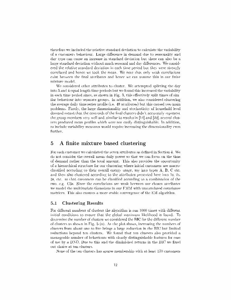
For di�erent numbers of clusters the algorithm is run 1000 times with di�erentinitial conditions to ensure that the global maximum likelihood is found. Todetermine the number of clusters we considered the BIC for the di�erent numberof clusters as shown in Fig. 5 (a). As the plot shows, increasing the numbers ofclusters from about one to �ve brings a large reduction in the BIC but limitedreductions beyond ten clusters. We found that ten clusters also provided amanageable number of behaviours with clearly distinguishable features for easeof use by a DNO. Due to this and the diminished returns in the BIC we �xedout choice at ten clusters.
None of the ten clusters has sparse membership with at least 170 customers
12
0 5 10 15 20 25 300.2
0.4
0.6
0.8
1
1.2
1.4
1.6
1.8x 10
4
Number of Clusters
Bay
esia
n In
form
atio
n C
riter
ion
(a)
1 2 3 4 5 6 7 8 9 100
100
200
300
400
500
600
Cluster
Num
ber
of C
usto
mer
s
Tariff ATariff BTariff CTariff DTariff ETariff W
(b)
Figure 5: (a) BIC for di�erent size clusters and (b) Numbers of customers pergroup in �nal clustering.
in each cluster as shown in Fig. 5 (b). Each bar is broken down in terms of thenumber of customers in each tari� from the Irish smart meter trial (see [17] formore details). Since no cluster is dominated by any tari� type then perhaps itcan be suggested that no signi�cantly new behaviours are created by di�erenttari� types.
The mean attributes of the �nal clusters are shown in Table 1 ordered interms of evening relative power. As shown from the second to �fth columns ofTable 1 many of the clusters can be distinguished by the mean overnight, break-fast, daytime and evening relative power values. Fig. 6 shows the normalizedmean daily pro�le from clusters 2, 4, 7 and 10 which show pro�les with largeaverage daytime, overnight, breakfast and evening demands respectively. Theclusters thus identify customers with heavy usage and high volatility at di�erenttime periods who could create violations of the low voltage network constraints.Some clusters have very similar mean pro�les, however these customers are dis-tinguishable by other attributes such as their seasonality (as with cluster 5 and6).
The clusters can be used to identify groups of customers who are suitablefor various demand reduction initiatives [18]. For example, from Table 1 wecan see that cluster 8 customers have high evening demand with low variability(as seen from the STD, seasonal and Weekend di�erence attributes). Suchcustomers could have their peak load reduced through the implementation ofstorage devices. Cluster 5 customers also have low variability in general yethave quite high seasonal di�erence in demand. Hence, such customers couldbe o�ered non-electric or more e�cient hearing alternatives in order to reducetheir Winter demand.
The clusters can also be useful for identifying customer behaviour types fromnon-energy based characteristics. We considered smart meter data from a sep-arate trial called the New Thames Valley Vision project2. This data consists
2See http://www.thamesvalleyvision.co.uk/ for more details.
13

Table 1: The mean value of each of the 7 attributes for each cluster.
AttributesCluster Overnight Breakfast Daytime Evening Mean STD Seasonal Week di�
1 0.72 1.11 1.07 1.21 1.18 3.47 1.262 0.44 0.80 1.45 1.29 0.53 1.05 0.763 0.75 0.78 1.06 1.31 0.42 0.81 0.444 0.90 0.75 0.85 1.34 0.60 1.61 0.635 0.58 0.78 1.17 1.40 0.76 2.37 0.616 0.55 0.74 1.17 1.44 0.48 0.93 0.657 0.56 1.24 0.94 1.48 0.59 1.22 1.438 0.67 0.68 0.93 1.56 0.49 0.98 0.749 0.44 0.70 1.10 1.65 0.53 1.01 0.9610 0.53 0.65 0.80 1.85 0.64 1.41 1.07
00:00 06:00 12:00 18:00 24:000.005
0.01
0.015
0.02
0.025
0.03
0.035
0.04
0.045
0.05
Time of Day
Nor
mal
ised
Dem
and
Cluster 2Cluster 4Cluster 7Cluster 10
Figure 6: Mean Daily pro�les for a selection of the �nal clusters.
of half-hourly smart meter data from 235 residential volunteers. We consid-ered a years worth of data beginning 27th February 2013 and assigned them tothe clusters (by calculating the posterior probabilities τi,j) using their derivedattributes. For the NTVV customers we also had access to the pro�le class in-formation and thus found that 70% of customers with overnight storage heaterswere members of cluster 1. This is unsurprising given the large relative season-ality score for this group. We note, that if we cluster the entire mean half hourlypro�le the �nal cluster pro�les are more similar and we miss certain features, forexample, the cluster consisting of large overnight demand. By construction, theclusters naturally identify customers who have heavy demand during particulartime periods of the day.
There is a small degree of subjectivity on the precise endpoints selected forthe time periods. To test how sensitive the �nal clusters are to small changes
14
0 0.1 0.2 0.3 0.4 0.5 0.6 0.7 0.80
20
40
60
80
100
120
140
160
180
Cou
nt
Classification Uncertainty 90% Quantile
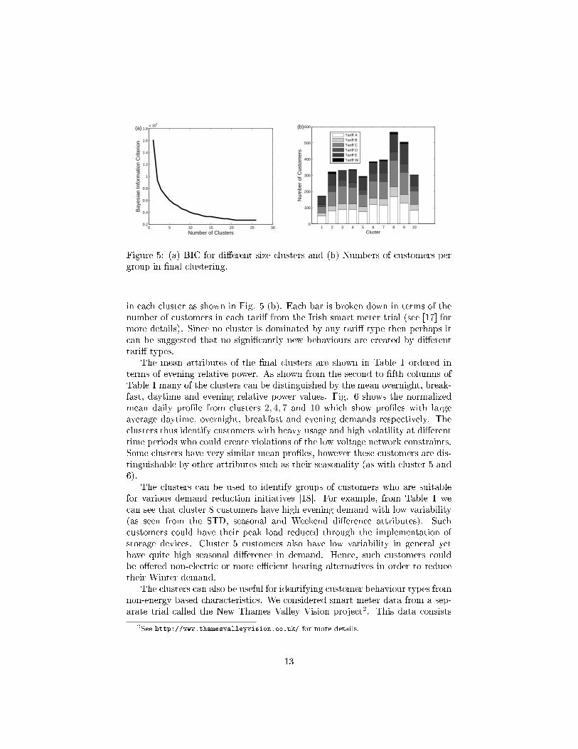
Figure 7: The 90% quantile of the classi�cation uncertainty from the bootstrapsamples for each customer.
in the boundary we implemented the clustering algorithm eight times (eachendpoint changed by a half hour earlier or later) to the same attributes butwith di�erent time periods. In each case the average change in cluster centreswas less than 6%. Hence the centres are similar when similar time periods arechosen and not too sensitive to changes in the endpoints.
5.2 Bootstrapping
We create M = 10, 000 bootstrap samples and consider the uncertainty measuresde�ned in Section 3.1 to test the reliability of the clustering. The entire processtook less than 2 hours on a basic desktop computer (single core processor at2.30GHz and 4GB RAM memory) and only 2 of the bootstraps did not con-verge which, since this is such a low number, were ignored. We �rst consider theclassi�cation uncertainty (1). This indicates how large our classi�cation uncer-tainty could be if the clusters had been de�ned di�erently. In Fig. 7 we reporton the worst 10% for each customer. The plot shows that there is a number ofcustomers without very certain clusters (close to 0.5) but there are an equallylarge number of customers who are very certain (close to zero). However, sincethis is the 90% quantile the average classi�cation uncertainty is much betterthan what is shown in the plot. The customers who tend to be uncertain mostlikely lie on the boundaries between multiple cluster centres. This is con�rmedby the fact that a large proportion of customers have a classi�cation uncertaintyof just less than 0.5 meaning that they are as likely to lie in all other clustersas lie in the most probable cluster.
Next we consider the Entropy given by equation (2). The entropy for theoriginal sample was E = 0.7972 and the mean over all bootstrap samples isE = 0.8056 with standard deviation 0.0063. The similarity of entropy valuesamongst all samples suggests that the entropy is not a�ected by sampling. Also,
15
crucially, all values are close to 1 suggesting that the clusters are well separatedand thus well de�ned.
Finally we considered the mean values over all bootstrap of each attribute foreach cluster. As mentioned in Section 3.1 due to potential mislabeling in eachclustered bootstrap we �rst matched the clusters centres in each bootstrap to theclosest (with respect to the Euclidean distance) centre in the original clusteringpresented in Table 1. We found that these mean clustered bootstrap samplesmatched the original mean centres given in Table 1 with all attribute meansagreeing to the �rst decimal place in all cases. In addition when considering thestandard deviation of each attribute in each cluster over all bootstraps none werelarger than 10% of the mean values given. This is unsuprising since consideringthe classi�cation uncertainty is small most customers had a de�nite clusterand thus a stable cluster centre from one bootstrap sample to the next. Thebootstrapping results con�rm that the majority of customers have been classi�edwith certainty. Hence, having assigned customers in the initial clustering wecan be con�dent that they belong to their respective clusters described by aparticular mean and covariance of our chosen attributes.
6 Summary
Large quantities of information about how customers use their energy is be-coming available through the uptake of smart meters. Clustering the mostimportant attributes of customers is a very common method for better under-standing the di�erent residential energy behaviours that exist and has manyapplications. In this paper we present a methodology for extracting, classifyingand then verifying the reliability of the �nal clustering. We began with detailedanalysis of smart meter data to identify some of the most important character-istics. In particular we analysed di�erent size demands and their distributionas a function of time-of-day and season. We identi�ed four key time periodswhich described di�erent peak demand behaviour, coinciding with common in-tervals of the day: overnight, breakfast, daytime and evening. We also foundthat demand in the di�erent time periods changed as a function of seasonalityand days of the week, thus identifying two major sources of variation. In addi-tion, we also included a mean normalized standard deviation of the demand asa measure of the irregularity of a customer. The time periods not only helpedus to model peak time behaviours and their variation but also allowed us to re-duce the number of attributes in our clustering implementation. We presenteda clustering of our chosen attributes into ten groups using a �nite mixture ofGaussian distributions. Such a method is commonly used in clustering but hasnot been explored in great detail within the power systems literature despitethe advantages over more common methods. We showed that the �nal clustersidenti�ed many important behaviours of the customers. As well as time periodsof greatest demand, we identi�ed those customers with the largest variabilityaccording to seasonality and weekend versus weekday di�erences. Understand-ing such changes in a customers seasonal behaviour can aid network operators
16

in longer term planning of the networks. Once we have assigned customers toa cluster we would like to evaluate how con�dent we are that the customersbelongs to the group they were assigned. That way we can be more con�dentthat the cluster centers are representative of the members. Such classi�cationuncertainty measures are not often included in the clustering power systemsliterature. Hence, we assessed the sample robustness of our clustering usingthree measures applied to several thousand bootstrapped samples. Following abootstrapping method presented in [11] we considered three measures of samplerobustness in our clustering We veri�ed that, assuming the underlying distribu-tion of the data is well approximated from the real data, the �nal clustering isreliable with a high degree of certainty of which customers belonged to whichcluster.
Natural extensions of the work is to incorporate the modelling of signi�cantlow carbon technologies into the clustering. Further work is especially needed totest the limits to which clustering can reduce the need for expensive monitoring.Previous work has shown the potential of linking demand attributes to publichousehold data [20]. Such, even weak, correlations can be utilized, together withother information, to more accurately model household level demand. Finally,many more smart meter-based trials are being produced in order to better un-derstand the LV network. Clustering, such as the one presented in this papercan be used to ensure representative customers have been monitored in suchtrials. Such methodology can potentially reduce costs and ensure that resultsare statistically signi�cant.
Acknowledgments
We wish to thank Scottish and Southern Energy Power Distribution (SSEPD)for their support via the New Thames Valley Vision Project (SSET203 NewThames Valley Vision), funded through the Low Carbon Network Fund.
References
[1] J. M. Abreu, F. P. Camara, and P. Ferrao. Using pattern recognition toidentify habitual behavior in residential electricity consumption. Energyand Buildings, 49:479�487, 2012.
[2] A. Albert and R. Rajagopal. Smart meter driven segmentation: Whatyour consumption says about you. IEEE Trans. Power Syst., 28:4019�4030, 2013.
[3] C. Beckel, L. Sadamori, T. Staake, and S. Santini. Revealing householdcharacteristics from smart meter data. Energy, 78:397�410, 2014.
[4] I. Benitez, A. Quijano, J-L. Diez, and I. Delgado. Dynamic clusteringsegmentation applied to load pro�les of energy consumption from spanishcustomers. Electrical Power and Energy Sys., 55:437�448, 2014.
17
[5] H. Cao, C. Beckel, and T. Staake. Are domestic load pro�les stable overtime? an attempt to identify target households for demand side manage-ment campaigns. In 39th Annual Conference of IEEE Industrial ElectronicsSociety (IECON 2013), pages 75�86, Vienna, Austria, 2013.
[6] M. Chaouch. Clustering-based improvement of nonparametric functionaltime series forecasting: Application to intra-day household-level loadcurves. IEEE Trans. Smart Grid, 5:411�419, 2014.
[7] G. Chicco. Overview and performance assessment of the clustering methodsfor electrical load pattern grouping. Energy, 42:68�80, 2012.
[8] G. Chicco and F. Piglione R. Napoli. Comparisons among clustering tech-niques for electricity customer classi�cation. IEEE Trans. Power Syst.,21:933�940, 2006.
[9] I. Dent, T. Craig, U. Aickelin, and T. Rodden. An approach for assessingclustering of households by electricity usage. In UKCI 2012, 12th AnnualWorkshop Comp. Intelligence, Heriot-Watt, UK, 2012.
[10] I. Dent, T. Craig, U. Aickelin, and T. Rodden. Finding the creatures ofhabit; clustering households based on their �exibility in using electricity.In Digital Futures 2012, Aberdeen, UK, 2012.
[11] J.G. Dias and J.K. Vermunt. Bootstrap methods for measuring classi�-cation uncertainty in latent class models, a. in rizzi and m. vichi (eds.).In COMPSTAT2006. Proc. Comp. Stats, Heidelberg: Physica/Springer-Verlag, pages 31�41, 2006.
[12] EA Technology. Assessing the impact of low carbon technologies on greatbritain's power distribution networks (last accessed june 2014), 2014.
[13] B. Efron. Bootstrap methods: Another look at the jackknife. Ann. Stats.,7:1�26, 1979.
[14] C. Flath, D. Nicolay, T. Conte, C. van Dinther, and L Filipova-Neumann.Cluster analysis of smart metering data - an implementation in practice.Bus. and Syst. Eng., 4:31�39, 2012.
[15] S. Haben, M. Rowe, D. V. Greetham, P. Grindrod, W. Holderbaum, B. Pot-ter, and C. Singleton. Mathematical solutions for electricity networks in alow carbon future. In CIRED 22nd International Conference on ElectricityDistribution, Stockholm, Sweden, 2013.
[16] S. Haben, J. A. Ward, D. V. Greetham, P. Grindrod, and C. Singleton. Anew error measure for forecasts of household-level, high resolution electricalenergy consumption. Int. J. of Forecasting, 30:246�256, 2014.
[17] Irish Social Science Data Archive. CER Smart Metering Project, 2012.
18

[18] J. Kwac, J. Flora, and R. Rajagopal. Household energy consumption seg-mentation using hourly data. IEEE Trans. Smart Grid, 5:420�430, 2014.
[19] G. McLachlan and D. Peel. Finite Mixture Models. Wiley Series in Proba-bility and Statistics, 2000.
[20] F. McLoughlin, A. Du�y, and M. Conlon. Characterising domestic elec-tricity consumption patterns by dwelling and occupant socio-economic vari-ables: An irish case study. Energy and Buildings, 48:240�248, 2012.
[21] J. Morley and M. Hazas. The signi�cance of di�erence: Understanding vari-ation in household energy consumption. In ECEEE 2011 Summer School,pages 2037�2046, Stockholm, Sweden, 2011.
[22] F. L. Quilumba, W. Lee, H. Huang, D. Y. Wang, and R.L. Szabados.Using smart meter data to improve the accuracy of intraday load forecast-ing considering customer behavior similarities. IEEE Trans. Smart Grid,6:911�918, 2014.
[23] T. Rasanen and M. Kolehmainen. Feature-based clustering for electricityuse time series data. Adaptive and Natural Computing Algorithms: LectureNotes in Computer Science, 5495:401�412, 2009.
[24] B. Stephen and S. J. Galloway. Domestic load characterization throughsmart meter advance strati�cation. IEEE Trans. Smart Grid, 3:1571�1572,2012.
[25] B. Stephen, A. J. Mutanen, S. J. Galloway, G. Burt, and P. Jentausta.Enhanced load pro�ling for residential network customers. IEEE Trans.Power Delivery, 29:88�96, 2014.
[26] J-P Zimmermann, M. Evans, J. Griggs, N. King, L. Harding, P. Roberts,and C. Evans. Household electricity survey: A study of domestic electricalproduct usage. Intertek Report R66141, 2012.
19