EIsJmER Applied Mathematics and Computation 100 (1999) 49-70

Analysis and approximation of optimal control problems for first-order elliptic

systems in three dimensions Max D. Gunzburger a**,1, Hyung-Chun Lee b72

a Department of Mathematics, Iowa State University, Ames, IA 50011-2064, USA b Department of Mathematics, Ajou University, Suwon, South Korea

Abstract

We examine analytical and numerical aspects of optimal control problems for first- order elliptic systems in three dimensions. The particular setting we use is that of div- curl systems. After formulating some optimization problems, we prove the existence and uniqueness of the optimal solution. We then demonstrate the existence of Lagrange multipliers and derive an optimality system of partial differential equations from which optimal controls and states may be deduced. We then define least-squares finite element approximations of the solution of the optimality system and derive optimal estimates for the error in these approximations. 0 1999 Elsevier Science Inc. All rights reserved.

Keywords: Optimal control; First-order systems; Finite element methods

1. Introduction

First-order elliptic systems arise in electromagnetics, fluid mechanics, and many other applications areas. Optimal control and optimization problems also arise in these connections. In this paper we study the latter type problem; in order to keep the exposition simple, we consider the particular context of

l Corresponding author. E-mail: gunzburg@iastate.edu. ’ Supported in part by the Air Force Office of Scientific Research under grant number F49620-9%

l-0407. * Supported in part by KOSEF 97-07-01-01-01-3 and the ‘96 Ajou University Faculty Research

Fund.

0096-3003/99/$ ~ see front matter 0 1999 Elsevier Science Inc. All rights reserved. PII: s0096-3003(98)00017-4

50 M.D. Gunzburger, H.-C. Lee I Appl. Math. Comput. 100 (19993 49-70

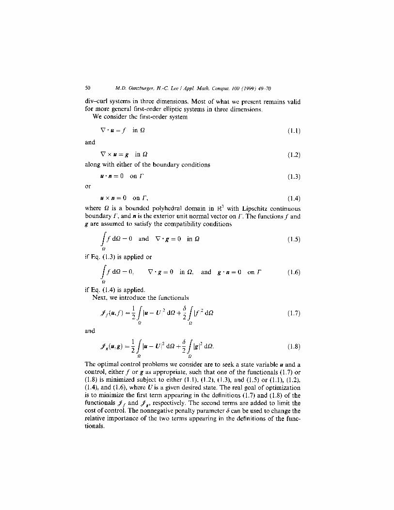
divxurl systems in three dimensions. Most of what we present remains valid for more general first-order elliptic systems in three dimensions.

We consider the first-order system

0.u=f in.0 (1.1)

and

Vxu=g inQ

along with either of the boundary conditions

u-n=0 onr

or

(1.2)

(1.3)

uxn=O onr, (1.4) where 52 is a bounded polyhedral domain in R3 with Lipschitz continuous boundary r, and n is the exterior unit normal vector on r. The functions f and g are assumed to satisfy the compatibility conditions

fdG=O and V-g=0 inSZ (1.5)

if Eq. (1.3) is applied or

J f dSZ=O> V-g=0 in52, and g. n = 0 on r (1.6) R

if Eq. (1.4) is applied. Next, we introduce the functionals

Cl.71

and

yg(u,g) = ; JIu - q* dC! +; JIgI’ dSZ. (1.8) l2 n

The optimal control problems we consider are to seek a state variable u and a control, either f or g as appropriate, such that one of the functionals (1.7) or (1.8) is minimized subject to either (l.l), (1.2), (1.3), and (1.5) or (l.l), (1.2), (1.4), and (1.6), where U is a given desired state. The real goal of optimization is to minimize the first term appearing in the definitions (1.7) and (1.8) of the functionals $f and yg, respectively. The second terms are added to limit the cost of control. The nonnegative penalty parameter 6 can be used to change the relative importance of the two terms appearing in the definitions of the func- tionals.

M.D. Gunzburger, H.-C. Lee I Appl. Math. Comput. 100 (1999) 49-70 51

T%e rYmct.<ana& anbcanr’ra& u.seaIu rtie opiim&aiiinprad&ns we &aveJi& defined are but examples of the many possibilities that can be treated by methods entirely similar to the ones used in this paper.

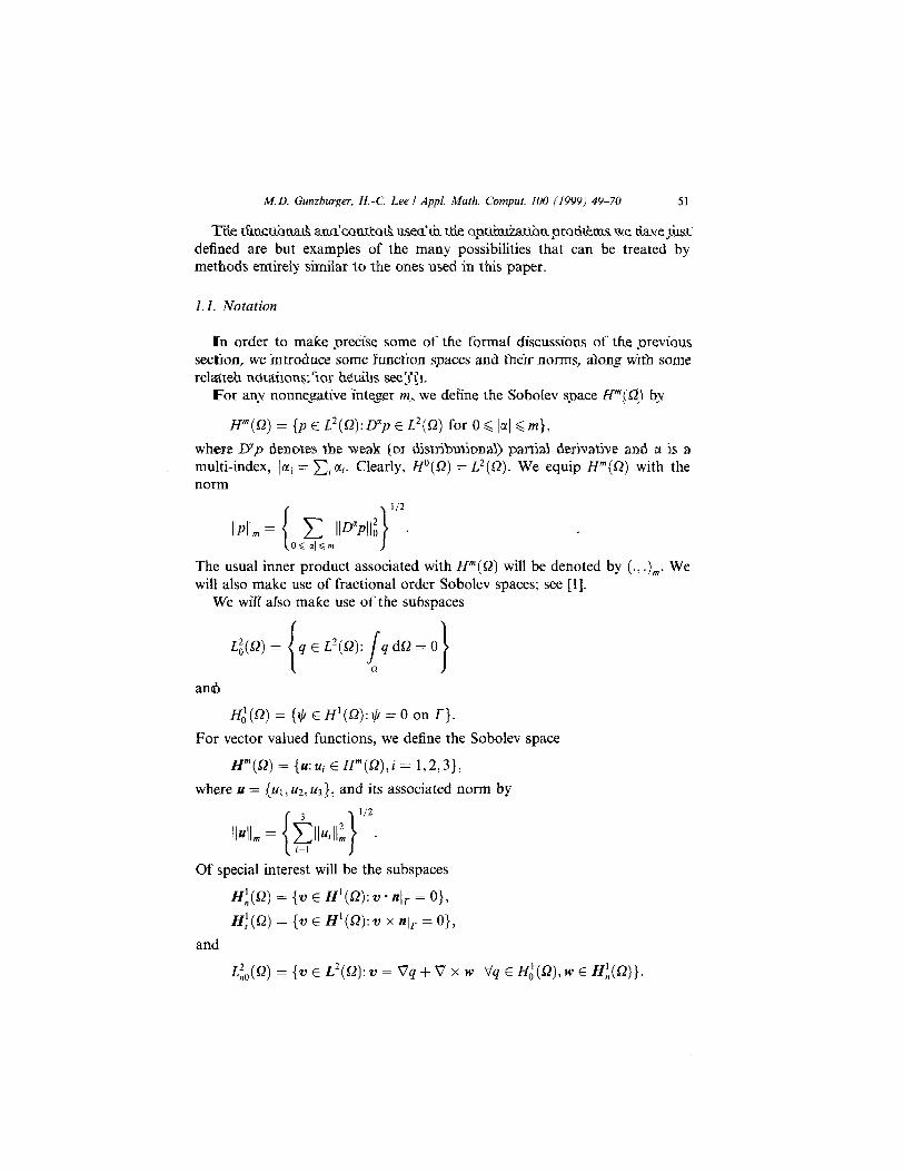
1.1. Notation

Hn order to make precise some af the formal discussions af the previous section, we introduce some function spaces and their norms, along with some relr&& n&&on~:?or &X&S seeIj<~

lFor anv nonnegative integer m,. we define the Sobolev space H”‘,CQj b>v

H”(s1) = (p E L2(sZ):D’p E L’(Q) for 0 < 11~1 GM},

where D”p denotes Ibe weak (or tisttibutiona>) partial derivative and tt is a multi-index, jell = Cj ai. Clearly, Ho(Q) = L*(Q). We equip H”(Q) with the norm

IiPll, = ( o<&P~P,l;}“2. .

The usual inner product associated with H”(Q) will be denoted by (.? .),. We will also make use of fractional order Sobolev spaces; see [l].

We will also make use of the subspaces

L;(Q) = q E L2(Q):

H,‘(Q) = {$ E H’(S2): rl/ = 0 on r}.

For vector valued functions, we define the Sobolev space

H”(Q) = {u:ui E H”(Q),i = 1,2,3},

where II = {ux.~uz~u~)., and its associated norm by

Of special interest will be the subspaces

H;(a) = {IJ E H’(S2): 2, -“Jr = O},

H#?) = {?I E II’( 21 x “lr = O},

and

L;,(Q) = {v E L2(!2): 21 = vq + v x w vq E H,‘(Q), w E H;(R)}.

52 MD. Gunzburger, H.-C. Lee I Appl. Math. Comput. 100 (1999) 49-70

All subspaces are equipped with the norms inherited from the underlying spaces.

2. Solvability results and optimal control problems for first-order elliptic systems

2.1. General systems

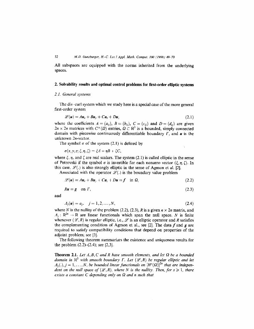
The divcurl system which we study here is a special case of the more general first-order system

di”(u) = Au, + Bu, + Cu, + Du, (2.1) where the coefficients A = (aV), B = (bij), C = (cij) and D = (dij) are given 2n x 2n matrices with CM(O) entries, Q c R3 is a bounded, simply connected domain with piecewise continuously differentiable boundary r, and u is the unknown 2n-vector.

The symbol o of the system (2.1) is defined by

+,Y,z; 5,v, i) = 5A + rlB + ic, where 5, q, and 5 are real scalars. The system (2.1) is called elliptic in the sense of Petrovski if the symbol (T is invertible for each nonzero vector (t, q, [). In this case, 9(.) is also strongly elliptic in the sense of Agmon et al. [2].

Associated with the operator 9(.) is the boundary value problem

2’(u) = Au, + Bu, + Cu, + Du := f in Q, (2.2)

Ru=g onr, (2.3) and

Aj(U) =aj, j= 1,2 ,..., N, (2.4) where N is the nullity of the problem (2.2), (2.3), R is a given n x 2n matrix, and /il : R2” -+ [w are linear functionals which span the null space. N is finite whenever (9, R) is regular elliptic, i.e., 9 is an elliptic operator and R satisfies the complementing condition of Agmon et al., see [2]. The data f and g are required to satisfy compatibility conditions that depend on properties of the adjoint problem; see [3].

The following theorem summarizes the existence and uniqueness results for the problem (2.2)-(2.4); see [2,3].

Theorem 2.1. Let A, B, C and R have smooth elements, and let Sz be u bounded domain in [w3 with smooth boundary r. Let (P’,R) be regular elliptic and let Aj(.),j = 1,. . . , N, be bounded linear functionals on [H”(s2)]2” that are indepen- dent on the null space of (3, R), where N is the nullity. Then, for s >, 1, there exists a constant C depending only on Q and n such that

M.D. Gunzburger, H.-C. Lee I Appl. Math. Comput. 100 (1999) 49-70 53

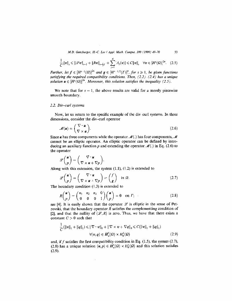
i IIvIIs G IIsv/Ipl + IIRvII+ + eInj(V)I G CIIUII, \Jv E P”(Q>l”. (2.5) j=l

Further, let f E [H”-‘(Q)]*” and g E [~‘-“*(r)]~, for s 3 1, be given functions satisfying the required compatibility conditions. Then, (2.2)-(2.4) has a unique solution u E [H’(Q)]‘“. A4 oreover, this solution satis$es the inequality (2.5).

We note that for s = 1, the above results are valid for a merely piecewise smooth boundary.

2.2. D&curl systems

Now, let us return to the specific example of the div-curl systems. In three dimensions, consider the div-curl operator

&i!(u)= ,“;: . ( > (2.6)

Since II has three components while the operator JY( .) has four components, J%! cannot be an elliptic operator. An elliptic operator can be defined by intro- ducing an auxiliary function p and extending the operator A(.) in Eq. (2.6) to the operator

p- = 0 (

V*ll

P > vxu+vp . Along with this extension, the system (1. l), (1.2) is extended to

y” = 0 ( V-u f

vxu+vp = g > 0 in 52. P

The boundary condition (1.3) is extended to

R u = 0 (

= 0 on r; P

(2.7)

(2.8)

see [4]. It is easily shown that the operator Y is elliptic in the sense of Pet- rovski, that the boundary operator R satisfies the complementing condition of [2], and that the nullity of (Z,R) is zero. Thus, we have that there exists a constant C > 0 such that

+Jll, + llqll1) < I/V - 410 f IIV x v + V~llrJ G cmll~ + 11~11,)

V’(v,q) E es9 x 4m (2.9)

and, if f satisfies the first compatibility condition in Eq. (1.5) the system (2.7), (2.8) has a unique solution (u,p) E H:(Q) x Hi(Q) and this solution satisfies (2.9).

54 M.D. Gunzbvrger, H.-C. Lee I Appl. Math. Comput. 100 (1999) 49-70

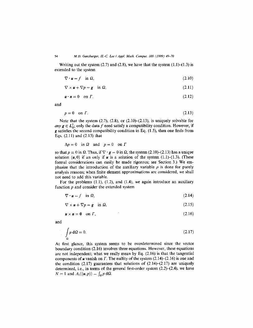
Writing out the system (2.7) and (2.8), we have that the system (1 .1)-(1.3) is extended to the system

V*u=f inR, (2.10)

V xu+Vp=g in Sz, (2.11)

u-n=0 onr, (2.12)

and

p=O on r. (2.13)

Note that the system (2.7), (2.8), or (2.10)-(2.13), is uniquely solvable for any g E L& only the data f need satisfy a compatibility condition. However, if g satisfies the second compatibility condition in Eq. (1..5), then one finds from Eqs. (2.11) and (2.13) that

Ap = 0 in Sz and p = 0 on r

so that p = 0 in 0. Thus, if V * g = 0 in 52, the system (2.lOt(2.13) has a unique solution (u, 0) if an only if II is a solution of the system (l.l)-(1.3). (These formal considerations can easily be made rigorous; see Section 3.) We em- phasize that the introduction of the auxiliary variable p is done for purely analysis reasons; when finite element approximations are considered, we shall not need to add this variable.

For the problems (1 .l), (1.2), and (1.4), we again introduce an auxiliary function p and consider the extended system

0.u=f inQ, (2.14)

V xu+Vp=g in Sz, (2.15)

uxn=O onr, (2.16)

and

s pdSZ=O.

R (2.17)

At first glance, this system seems to be overdetermined since the vector boundary condition (2.16) involves three equations. However, these equations are not independent; what we really mean by Eq. (2.16) is that the tangential components of u vanish on r. The nullity of the system (2.14~(2.16) is one and the condition (2.17) guarantees that solutions of (2.14H2.17) are uniquely determined, i.e., in terms of the general first-order system (2.2)-(2.4), we have N = 1 and A, ((u,p)) = Jnp dL?.

M.D. Gumburger, H.-C. Lee I Appl. Math. Comput. 100 (1999) 49-70

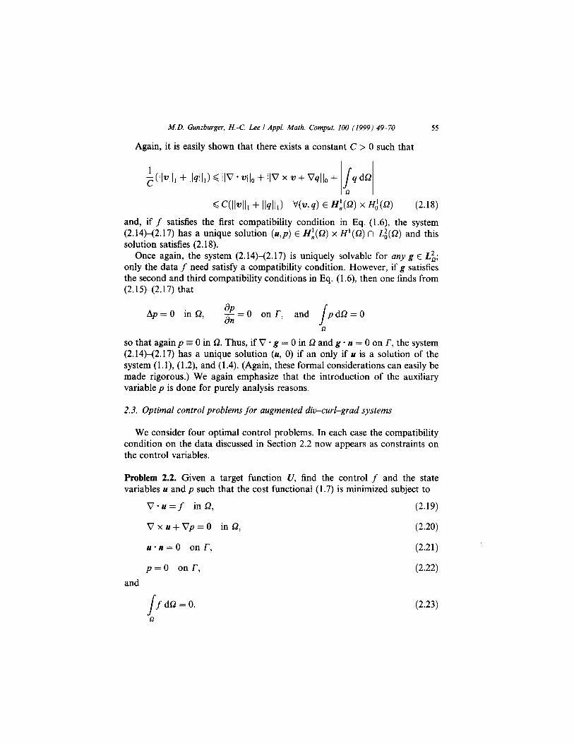
Again, it is easily shown that there exists a constant C > 0 such that

55

G C(II4II + 11~111) v?q) E em x fm-3 (2.18)

and, if f satisfies the first compatibility condition in Eq. (1.6) the system (2.14)-(2.17) has a unique solution (u,p) E H:(Q) x H’(Q) n L;(Q) and this solution satisfies (2.18).

Once again, the system (2.14)-(2.17) is uniquely solvable for any g E Li; only the data f need satisfy a compatibility condition. However, if g satisfies the second and third compatibility conditions in Eq. (1.6), then one finds from (2.15)-(2.17) that

Ap = 0 in a, 8P an = 0 on r, and s

pdO=O R

so that again p s 0 in 0. Thus, if V - g = 0 in D and g * n = 0 on r, the system (2.14)-(2.17) has a unique solution (u, 0) if an only if u is a solution of the system (1. l), (1.2), and (1.4). (Again, these formal considerations can easily be made rigorous.) We again emphasize that the introduction of the auxiliary variable p is done for purely analysis reasons.

2.3. Optimal control problems for augmented d&curl-grad systems

We consider four optimal control problems. In each case the compatibility condition on the data discussed in Section 2.2 now appears as constraints on the control variables.

Problem 2.2. Given a target function U, find the control f and the state variables u and p such that the cost functional (1.7) is minimized subject to

V*u=f inSZ, (2.19)

Vxu+Vp=O in.0, (2.20)

u-n=0 onr, (2.21)

p=O onr, (2.22)

and

J f dQ=O. 51

(2.23)

56 MD. Gumburger, H.-C. Lee I Appl. Math. Comput. 100 (1999) 49-70

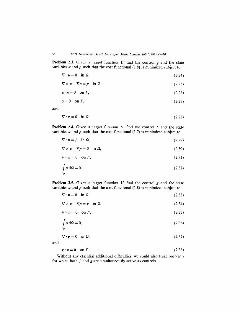
Problem 2.3. Given a target function U, find the control g and the state variables u and p such that the cost functional (1.8) is minimized subject to

V-u=0 inC?, (2.24)

Vxu+Vp=g inQ, (2.25)

u-n=0 onr, (2.26)

p=O on r, (2.27)

and

V*g=O inS1. (2.28)

Problem 2.4. Given a target function U, find the control f and the state variables u and p such that the cost functional (1.7) is minimized subject to

V*u=f in51, (2.29)

Vxu+Vp=O in@ (2.30)

uxn=O onr,

J pdCJ=O.

a

(2.31)

(2.32)

Problem 2.5. Given a target function U, find the control g and the state variables u and p such that the cost functional (1.8) is minimized subject to

V-u=0 in51, (2.33)

Vxu+Vp=g inL?, (2.34)

uxn=O onr,

s pdSZ=O,

n

(2.35)

(2.36)

V-g=0 inQ, (2.37)

and

g-n=0 onr. (2.38)

Without any essential additional difficulties, we could also treat problems for which both f and g are simultaneously active as controls.

M.D. Gumburger, H.-C. Lee I Appl. Math. Comput. 100 (1999) 49-70 57

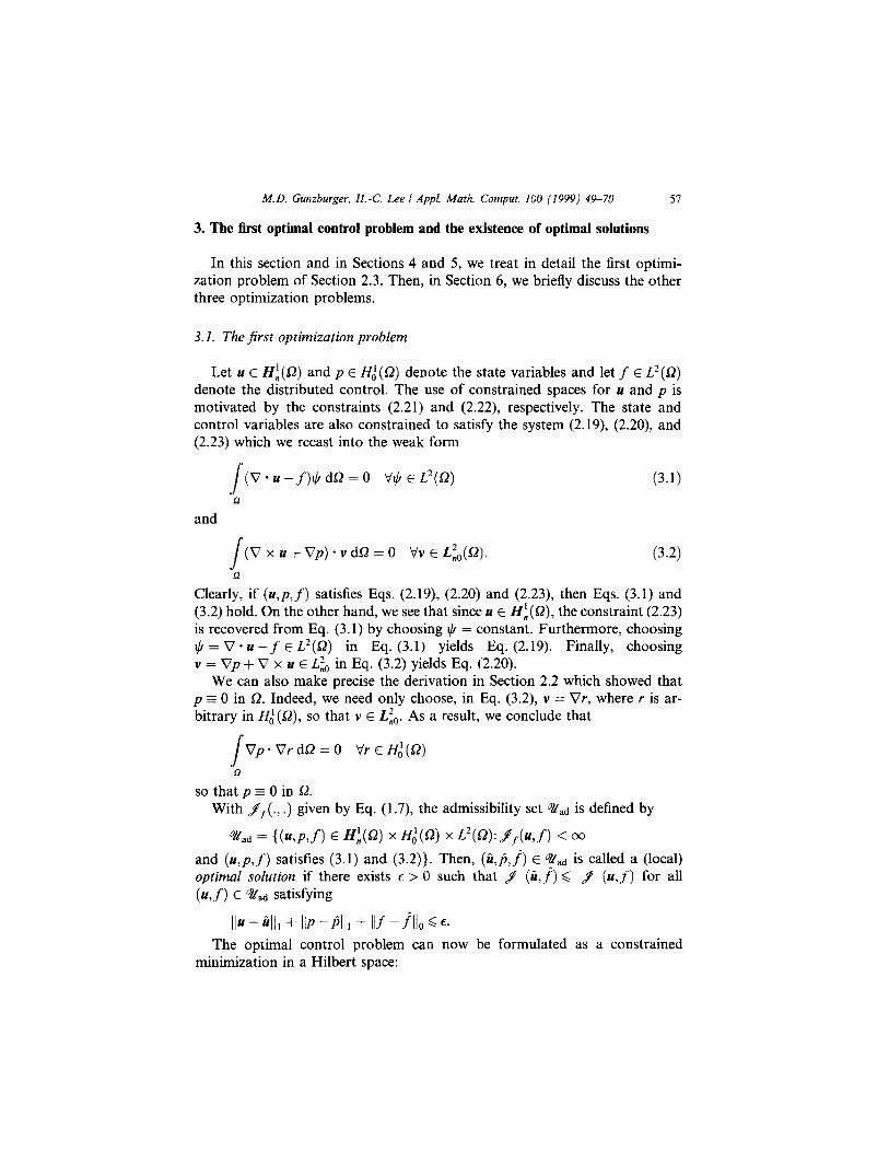
3. The first optimal control problem and the existence of optimal solutions

In this section and in Sections 4 and 5, we treat in detail the first optimi- zation problem of Section 2.3. Then, in Section 6, we briefly discuss the other three optimization problems.

3.1. TheJirst optimization problem

Let u E Hi (s2) and p E Hi (Q) denote the state variables and let f E L2 (52) denote the distributed control. The use of constrained spaces for u and p is motivated by the constraints (2.21) and (2.22) respectively. The state and control variables are also constrained to satisfy the system (2.19), (2.20), and (2.23) which we recast into the weak form

I (V-u-f)+dSZ=O V$EL*(SZ) (3.1)

a and

I (Vxu+Vp)*vdQ=O ‘vGL$(Q).

R (3.2)

Clearly, if (u,p,f) satisfies Eqs. (2.19), (2.20) and (2.23), then Eqs. (3.1) and (3.2) hold. On the other hand, we see that since u E Hi(Q), the constraint (2.23) is recovered from Eq. (3.1) by choosing Ic/ = constant. Furthermore, choosing rj = V. u -f E L*(Q) in Eq. (3.1) yields Eq. (2.19). Finally, choosing v = Vp + V x u E Lfo in Eq. (3.2) yields Eq. (2.20).

We can also make precise the derivation in Section 2.2 which showed that p = 0 in 52. Indeed, we need only choose, in Eq. (3.2), v = Vr, where r is ar- bitrary in H,(Q), so that v E Li,,. As a result, we conclude that

I Vp-VrdQ=O Vr#(Q) R

so that p E 0 in s2. With yf(., .) given by Eq. (1.7), the admissibility set @ad is defined by

@ad = {b,p,f) E@(Q) xH,'(Q) xL2(s2):kPf(u~f) <O" and (u,p,f) satisfies (3.1) and (3.2)). Then, (li,@,f^) E Fad is called a (local) optima2 solution if there exists 6 > 0 such that $ (i,f) ,< 9 (u, f) for all (u, f) E @ad satisfying

IIU - 41, + IIP -Al1 + Ilf -Al, G c. The optimal control problem can now be formulated as a constrained

minimization in a Hilbert space:

58 M.D. Gunzburger, H.-C. Lee I Appl. Math. Comput. 100 (1999) 49-70

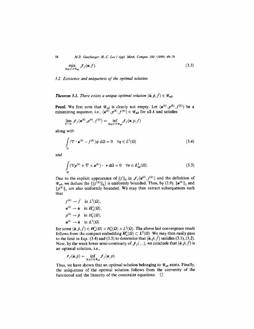
(3.3)

3.2. Existence and uniqueness of the optimal solution

Theorem 3.1. There exists a unique optimal solution (i,i,f) f ad.

Proof. We first note that @ad is clearly not empty. Let (&),p@),f@)) be a minimizing sequence, i.e., (u@),p@), j+)) E %,d for all k and satisfies

along with

I (V.~(~)-f(~))tjdQ=O b’qEL2(8) R

(3.4)

and

I ( Vpck) + V x ~(~1) * v d1;2 =: 0 Vv E L;,(L?). (3.5)

0

Due to the explicit appearance of ljj$, in yJ~(~),f(~)) and the definition of @ad, we deduce the { Ilf(k) II,,} is uniformly bounded. Then, by (2.9), IIu(~)II, and IIP(~) II, are also uniformly bounded. We may then extract subsequences such that

fck) - J: in L2(sZ) > #) - ri in H:(Q), p(k) -$ in Hi(Q),

U(k) -+ ir in L2(Q)

for some (ri, @, f*) E Hi (52) x H,’ (52) x L2 (52). The above last convergence result follows from the compact embedding Hf, (Q) c L2( a). We-may then easily pass to the limit in Eqs. (3.4) and (3.5) to determine that (G,fi,f) satisfies (3.1), (3,2). Now, by the weak lower semi-continuity of y,-(., .), we conclude that (ti,$,f) is an optimal solution, i.e.,

of = ( *y* /f(UYP). 4 a Thus, we have shown that an optimal solution belonging to %ad exists. Finally, the uniqueness of the optimal solution follows from the convexity of the functional and the linearity of the constraint equations. 0

M.D. Guruburger, H.-C. Lee I Appl. Math. Comput. 100 (1999) 49-70 59

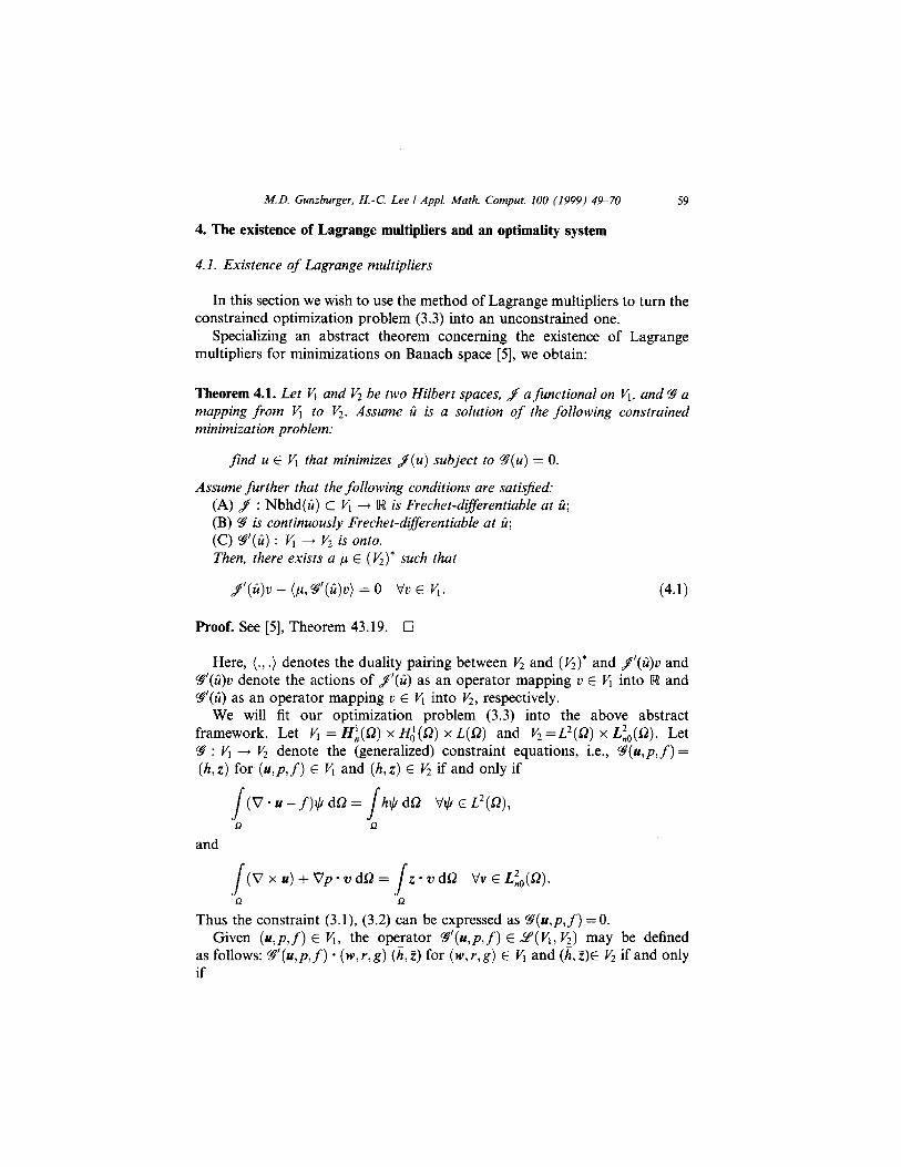
4. The existence of Lagrange multipliers and an optimality system

4.1. Existence of Lagrange multipliers

In this section we wish to use the method of Lagrange multipliers to turn the constrained optimization problem (3.3) into an unconstrained one.

Specializing an abstract theorem concerning the existence of Lagrange multipliers for minimizations on Banach space [5], we obtain:

Theorem 4.1. Let P$ and V, be two Hilbert spaces, f a functional on 6, and 23 a mapping from VI to V2. Assume i2 is a solution of the following constrained minimization problem:

find u E fi that minimizes f(u) subject to 9(u) = 0.

Assume further that the following conditions are satisfied: (A) f : Nbhd(li) c V, -+ R is Frechet-differentiable at ti; (B) Y is continuously Frechet-dtferentiable at li; (C) S’(i) : V, --f V2 is onto. Then, there exists a p E (Q)* such that

y(ii)v - (p, ~‘(iql) = 0 vu E fi. (4.1)

Proof. See [5], Theorem 43.19. 0

Here, (., .) denotes the duality pairing between V, and (IQ* and f’(l;)u and ?J’(fi)u denote the actions of I’(C) as an operator mapping v E V, into R and %‘(ti) as an operator mapping v E V, into 6, respectively.

We will fit our optimization problem (3.3) into the above abstract framework. Let V, = Hi(a) x H:(Q) x L(Q) and V, =L2(Q) x L$,(Q). Let 3 : VI -+ V2 denote the (generalized) constraint equations, i.e., g(u,p, f) = (h,z) for (u,p, f) E V, and (h,z) E V, if and only if

s (V-u-f)$dO=

J h+ dS2 V$ E L*(Q),

R a and

J (Vxu)+Vp.vddSZ= J z.wdO V~EL;,(Q). a R Thus the constraint (3.1), (3.2) can be expressed as 9(u,p, f) =O.

Given (u,p, f) E V,, the operator @(u,p, f) E Z( l$, I$) may be defined as follows: Y(u,p, f) - ( w, r, g) (h, Z) for (w, r, g) E fi and (h, Z)E I$ if and only if

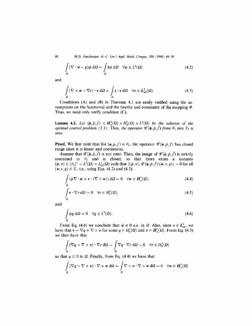
60 M.D. Gunzburger, H.-C. Lee I .4ppl. Math. Comput. 100 (1999) 49-70

I (V-w-g)$dS2= I

hll/dSZ VlII/ ELM 0 $2

(4.2)

and

I (‘17 x w+Vr)*vdQ=

I z * v dQ Vv E L;,(G?). (4.3)

R 0 Conditions (A) and (B) in Theorem 4.1 are easily verified using the as-

sumptions on the functional and the linerity and continuity of the mapping 9. Thus, we need only verify condition (C).

Lemma 4.2. Let (i&e,{) E H:(Q) x H,(Q) x L2(a) be the soZution of the optimal control problem (3.3). Then, the operator @(i&&f) from 6 into y2 is onto.

Proof. We first note that for (u,p,j”) E 6, the operator ‘#(u,p,f) has closed range since it is linear and continuous.

Assume that ?J’(ii,jj,f^) is not onto. Then, the image of s’(li,@,f) is strictly contained in V2 and is closed, so that there exists a nonzero (II/, v) E (v2)* = L2(Q) x L&(Q) such that ((+, v), Y’(b,@,f^)*(w, r,g)) = 0 for all (w, r, g) E V,! i.e., using Eqs. (4.2) and (4.3),

s ($V*w+v*(Vxw))dQ=O ‘%vEH;(o), R

I v*VrdSZ=O b-EH;(Q),

0

(4.4)

(4.5)

and

J’ t,bg dQ = 0 Yg E L2(Q). (4.6) a

From Eq. (4.6) we conclude that $ = 0 a.e. in 0. Also, since v E I,:,, we have that v = Vq + V x v for some q E H;(0) and v E H!,(Q). From Eq. (4.5) we then have that

s (Vq+Vxv).VrdL?=

s Vq*VrdQ=O VrEHj(52)

R n so that q = 0 in 52. Finally, from Eq. (4.4) we have that

J (Vq+Vxv).VxwdQ= J Vxv*VxwdQ=O VWEH@)

R R

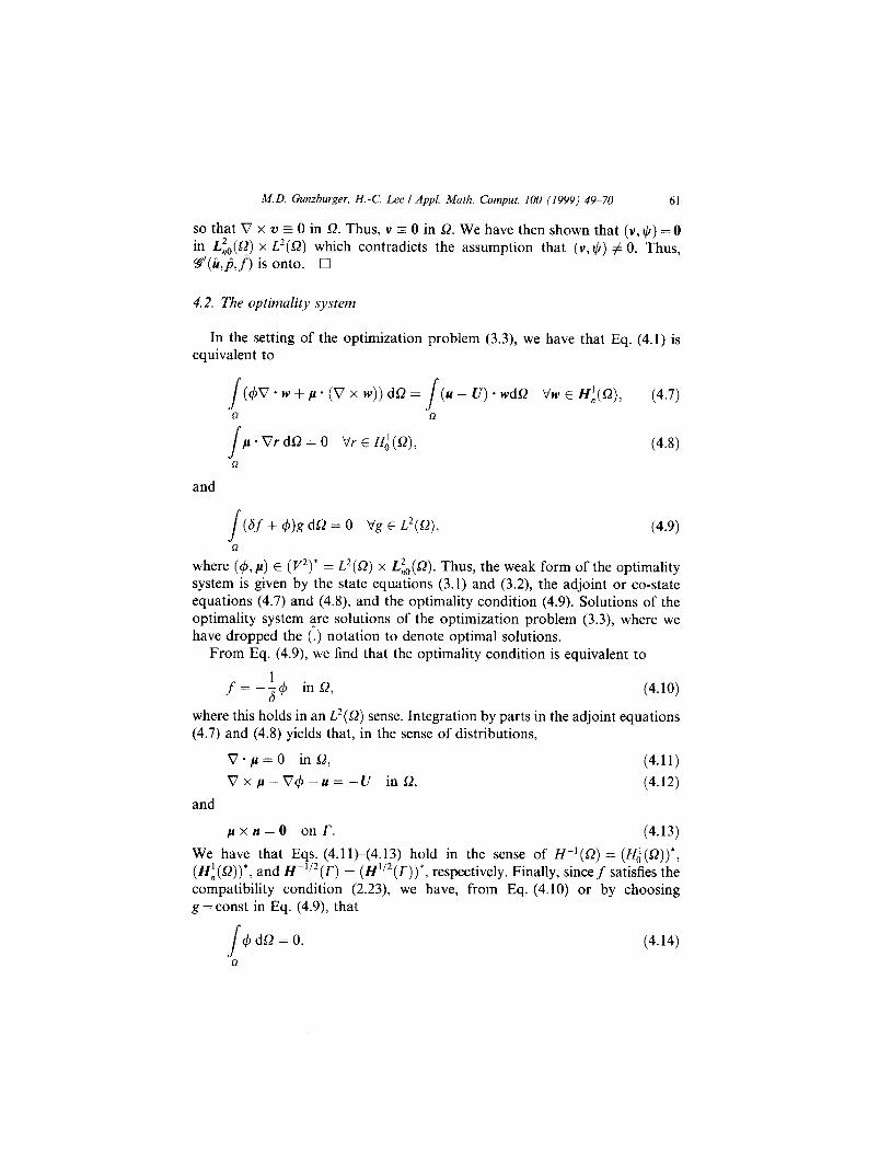
M.D. Gunzburger, H.-C. Lee I Appl. Muth. Comput. 100 f1999) 49-70 61

so that V x v =: 0 in Q. Thus, v = 0 in G. We have then shown that (v, $) = 0 in L&(Q) x L’(Q) which contradicts the assumption that (v, $) # 0. Thus, 9+(li,$:f) is onto. q

4.2. The optimality system

In the setting of the optimization problem (3.3), we have that Eq. (4.1) is equivalent to

s (+V*w+p*(Vxw))dSZ= s

(u-Li’).wdQ VwG@), (4.7) 0 R

(4.8)

and

J (Sf + 4)g dQ = 0 Vg E L*(Q), (4.9)

R where (4, p) E (I”)* = L*(Q) x L&(Q). Thus, the weak form of the optimality system is given by the state equations (3.1) and (3.2), the adjoint or co-state equations (4.7) and (4.8), and the optimality condition (4.9). Solutions of the optimality system are solutions of the optimization problem (3.3), where we have dropped the (.) notation to denote optimal solutions.

From Eq. (4.9), we find that the optimality condition is equivalent to

j-++ in 52, (4.10)

where this holds in an L2(.Q) sense. Integration by parts in the adjoint equations (4.7) and (4.8) yields that, in the sense of distributions,

V-p=0 inn, (4.11)

Vxp-VC$-u=-U ina, (4.12)

and

pxn=O onf. (4.13)

We have that Eqs. (4.11)-(4.13) hold in the sense of H-‘(Q) = (Hd(Q))*, (Hi(Q))*, and H-“‘(r) = (H”2(r))*, respectively. Finally, since f satisfies the compatibility condition (2.23), we have, from Eq. (4.10) or by choosing g=const in Eq. (4.9), that

s $dL’=O. (4.14)

0

62 MD. Gwtzburger, H.-C. Lee I Appl. Math. Comput. 100 (1999) 49-70

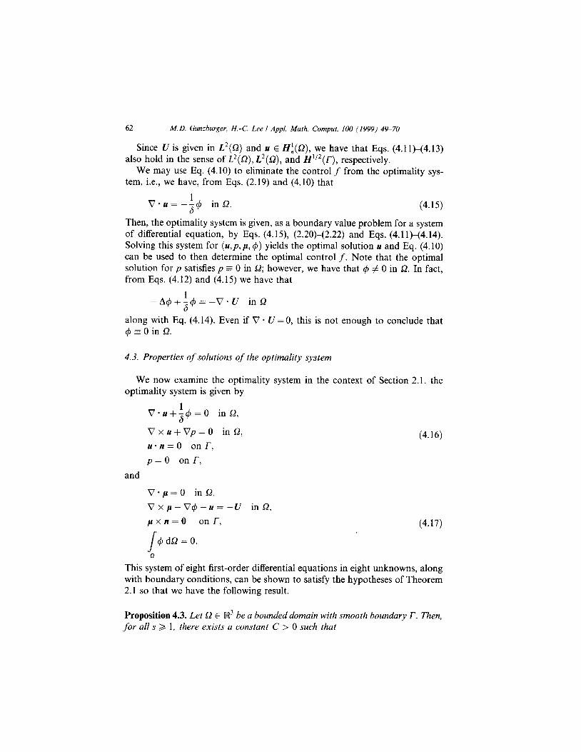
Since U is given in L’(G) and II E Hi(Q), we have that Eqs. (4.11)-(4.13) also hold in the sense of L’(Q), L2(Q), and H’j2(Q, respectively.

We may use Eq. (4.10) to eliminate the control f from the optimality sys- tem, i.e., we have, from Eqs. (2.19) and (4.10) that

V-u= --id, in 52. (4.15)

Then, the optimality system is given, as a boundary value problem for a system of differential equation, by Eqs. (4.15), (2.20)-(2.22) and Eqs. (4.11)<4.14). Solving this system for (~,p, p, C#J) yields the optimal solution u and Eq. (4.10) can be used to then determine the optimal control f. Note that the optimal solution for p satisfies p z 0 in Q; however, we have that 4 # 0 in s2. In fact, from Eqs. (4.12) and (4.15) we have that

-Ac/J+~c$=-V*U in52

along with Eq. (4.14). Even if V * U = 0, this is not enough to conclude that 4 E 0 in 52.

4.3. Properties of solutions of the optimality system

We now examine the optimality system in the context of Section 2.1. the optimality system is given by

Vxu+Vp=O in52,

u-n=0 onr,

p=O on r,

(4.16)

and

V-p=0 inQ,

Vxp-V$--u=-U in!&

pxn=o on r! (4.17)

J 4dL?=O.

This system of eight first-order differential equations in eight unknowns, along with boundary conditions, can be shown to satisfy the hypotheses of Theorem 2.1 so that we have the following result.

Proposition 4.3. Let 52 E R” be a bounded domain with smooth boundary r. Then, for all s 2 1, there exists a constant C > 0 such that

M.D. Gunzburger, H.-C. Lee I Appl. Math. Comput. 100 (1999) 49-70

+ IlV x v + Vqlls-, S-l

63

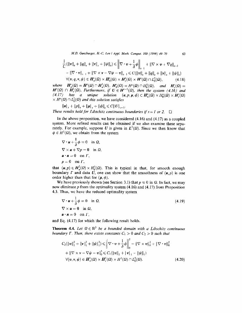
+ IIV * VII,4 + IIV x v - w - 4-1 G cm4ls + llf311, + ll~lls + 11w v’(v, 4, v, II/) E H”,(Q) x H;(Q) x H;(Q) x H”(Q) n Jg(f-4, (4.18)

where H”,(Q) = H”(G) nH~(!G), H;(O) = fP(s2) nH;(Q), and H;(Q) = H”(Q) n H:(Q). Furthermore, if U E H”-‘(Q), then the system (4.16) and (4.17) has a unique solution (u,P,P, 4) E H”,(Q) x H,“(Q) x H;(Q) x H”(Q) n L:(Q) and this solution satisjies

l141s + IIPII, + llPlls + 11411, G CII ~II,-,~ These results hold for Libschitz continuous boundaries ifs = 1 or 2. 0

In the above proposition, we have considered (4.16) and (4.17) as a coupled system. More refined results can be obtained if we also examine these sepa- rately. For example, suppose U is given in L’(0). Since we then know that CJ~ E H’(a), we obtain from the system

Vxu+Vp=O in@ u*n=O onr, p= 0 on F,

that (u,p) E Hi(Q) x Hi(Q). Th’ 1s is typical in that, for smooth enough boundary r and data U, one can show that the smoothness of (u,p) is one order higher than that for (p, 4).

We have previously shown (see Section 3.1) that p = 0 in L?. In fact, we may now eliminate p from the optimality system (4.16) and (4.17) from Proposition 4.3. Thus, we have the reduced optimality system

V.rr+i~$=O inO, (4.19)

Vxu=O inn, u-n=0 onr,

and Eq. (4.17) for which the following result holds.

Theorem 4.4. Let 52 E 0X3 be a bounded domain with a Libschitz continuous boundary r. Then, there exists constants Cl > 0 and C2 > 0 such that

G(ll4: + IIVII: + 11~11:) G /v . v + -igill; + 110 x 4; + 118 .vlI:

+ IlV x v - w - 4; ~~l(llvlll + IIVII, + IMI,) V(v,v,t,b) E H;(Q) x H:(Q) x If’@) fIL;(Q). (4.20)

64 M.D. Gumburger, H.-C. Lee I Appl. Math. Comput. 100 (1999) 49-70

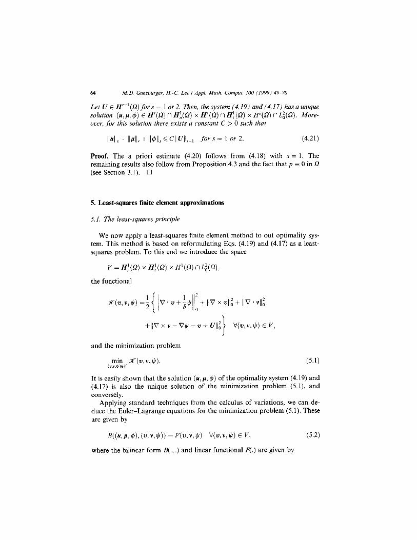
Let U E H”-’ (52) f or s = 1 or 2. Then, the system (4. I9) and (4.17) has a unique solution (u, p, 4) E H”(Q) n Hi(a) x H”(Q) n Hi (52) x H”(Q) n L:(Q). More-

over, for this solution there exists a constant C > 0 such that

I/4,7 + IIPII, + 11d41, G CII m, for s = 1 or 2. (4.21)

Proof. The a priori estimate (4.20) follows from (4.18) with s = 1. The remaining results also follow from Proposition 4.3 and the fact that p = 0 in Q (see Section 3.1). 0

5. Least-squares finite element approximations

5.1. The least-squares principle

We now apply a least-squares finite element method to out optimality sys- tem. This method is based on reformulating Eqs. (4.19) and (4.17) as a least- squares problem. To this end we introduce the space

V = H$2) x H,!(0) x H’(O) r-d@),

the functional

fllVXV-VIC/-w+q; V(W? v, $) E v,

and the minimization problem

It is easily shown that the solution (u, p, 4) of the optimality system (4.19) and (4.17) is also the unique solution of the minimization problem (5.1), and conversely.

Applying standard techniques from the calculus of variations, we can de- duce the Euler-Lagrange equations for the minimization problem (5.1). These are given by

B((u, P, 4)1 (V! v, II/)) = F(v, v, $1 VW, v, $1 E v,

where the bilinear form B(., .) and linear functional F(.) are given by

(5.4

M.D. Gunzburger, H.-C. Lee I Appl. Marh. Comput. 100 (1999) 49-70 65

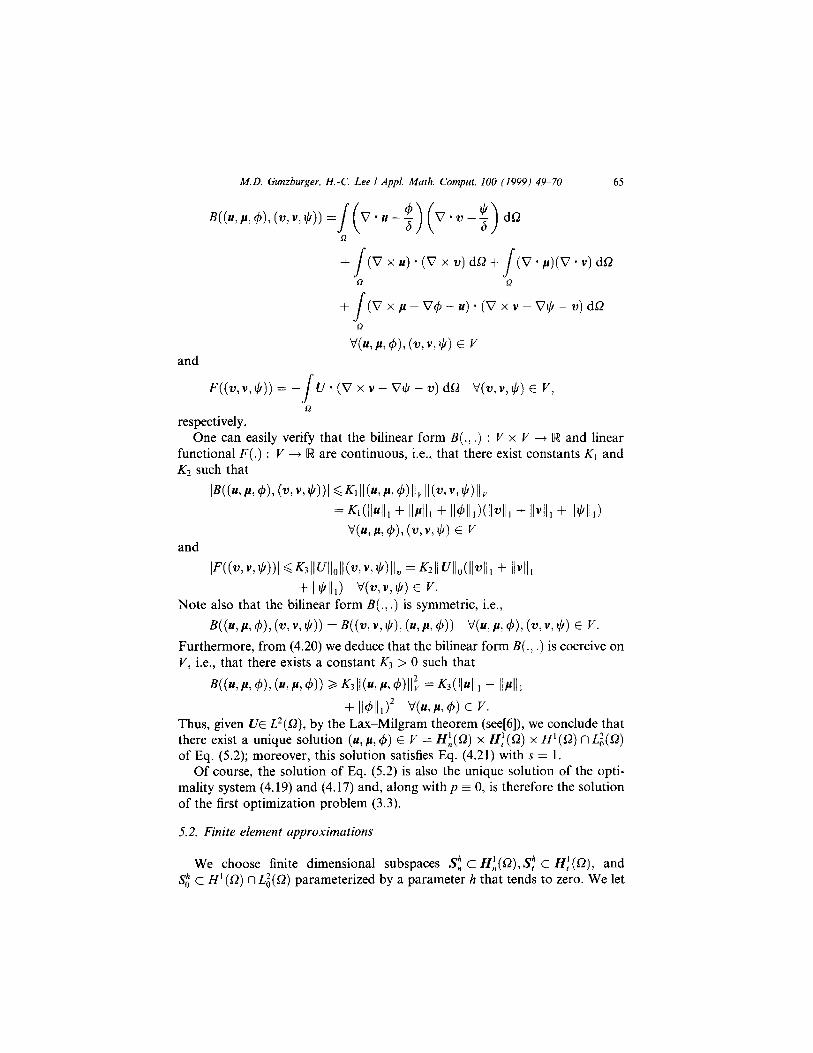
B((u, P, $11 (VI “7 II/)) = J(v.u-~)(v*w-$)dR R

+ (Vxu).(Vxv)dQ+ s J (V.p)(V.v)dQ 0 R

+ (Vxp-V4-u).(Vxv-Vt,-w)dS2 J R and

F((%“,$)) = - J fJ* (V xv-V+-v)dS2 V(v,v,t,h)~ Y,

n respectively.

One can easily verify that the bilinear form B(., .) : V x V + R’ and linear functional F(.) : V -+ IR are continuous, i.e., that there exist constants K, and K2 such that

I~~~~~~!~~,~~:“~~~~l6~lIl~~~~~~~II,II~~~~”~~~I/~

= ~l(II4, + lIPIll -IF ll4ll1)wll, + Ibill + IIII/Il,)

V(U> P, 41, (v, “!$I (5 Jf and

I~((~~“~~))l~~3II~ll~ll~~~“~rl/~ll. = ~2II~ll0(ll~lll + IMI, + ll$ll,) WU?Y,$) E v.

Note also that the bilinear form B(.: .) is symmetric, i.e.,

B((u, B: 41, (Y “> $1) = B(( w, “, $), (K B, 4)) v’(u, P: 4), (VT “, $1 E v. Furthermore, from (4.20) we deduce that the bilinear form B(., .) is coercive on V, i.e., that there exists a constant K3 > 0 such that

~((~,P,~),(~:P,~)) ~~3IlbwdGII: =K3(llulll + 11~11,

+ 11~11,)2 Yu, cc, 4) E y. Thus, given UE L’(Q), by the Lax-Milgram theorem (see[6]), we conclude that there exist a unique solution (u,c(, 4) E V = Hi(Q) x Hf(SZ) x H’(Q) nLi(SZ) of Eq. (5.2); moreover, this solution satisfies Eq. (4.21) with s = 1.

Of course, the solution of Eq. (5.2) is also the unique solution of the opti- mality system (4.19) and (4.17) and, along with p = 0, is therefore the solution of the first optimization problem (3.3).

5.2. Finite element approximations

We choose finite dimensional subspaces Si c HA(O), S: c H,! (Q), and s; c P(i2) nL;(n) p arameterized by a parameter h that tends to zero. We let

66 M.D. Gtmzburger, H.-C. Lee I Appl. Math. Comput. 100 (1999) 49-70

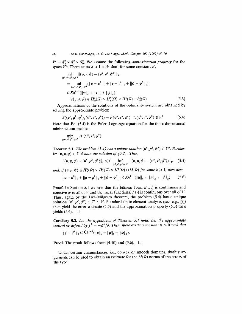
Vh = Sh x SF x Si. We assume the following approximation property for the space i”: There exists k > 1 such that, for some constant K,

inf II(w,v,$) - (~~,v~,ll/~)ll~ (vh.ti.@)& = td,“f$vr(ll~ - VhllL + lb - Vhlll + IW - Il/%)

~~~k-‘(II~llk + IlVllk + IIIclllk) V(w,v, I/?) E H;(R) x Hf(b2) x fP(SZ) n L;(Q). (5.3)

Approximations of the solutions of the optimality system are obtained by solving the approximate problem

B((u”,a”,~“),(w”,v”,Il/h)) =F(wh,vh,@) v(wh,vh,$h) E Vh. (5.4) Note that Eq. (5.4) is the Euler-Lagrange equation for the finite-dimensional minimization problem

min (vh.vh,lp)Ev”

Xx(&, vh, $“).

Theorem 5.1. Theproblem (5.4) has a unique solution (r#, ph, 4h) E Vh. Further, let (u,c(,$) E V denote the solution of (5.2). Then,

II(u,p,4) - (~,$,ah)lly~c,,,“i~~i,, II(UIII~4) - (~h~Vhdmlv (5.5)

and, $ (u, p, $) E Hff(s2) x H:(Q) x H&(a) f~ L;(G) for some k > 1, then also

(1~ - $11, + lllc -B~II~ + II4 - 4% ~~hk-‘W41, + llall~ + Il4ll/J (5.6)

Proof. In Section 5.1 we saw that the bilinear form B(., .) is continuous and coercive over all of V and the linear functional F(.) is continuous over all of V. Thus, again by the Lax-Milgram theorem, the problem (5.4) has a unique solution (r#, ph, @) E Vh c V. Standard finite element analyses (see, e.g., [7]) then yield the error estimate (5.5) and the approximation property (5.3) then yields (5.6). 0

Corollary 5.2. Let the hypotheses of Theorem 5.1 hold. Let the approximate control be defined by fh = -@h,J6. Then, there exists a constant I? > 0 such that

IV -f% G~hk-‘(I141k + IIPL + ll4lld

Proof. The result follows from (4.10) and (5.6). 0

Under certain circumstances, i.e., convex or smooth domains, duality ar- guments can be used to obtain an estimate for the L’(Q) norms of the errors of the type

M.D. Gunzburger, H.-C. Lee I Appl. Math. Cornput. 100 (1999) 49-70

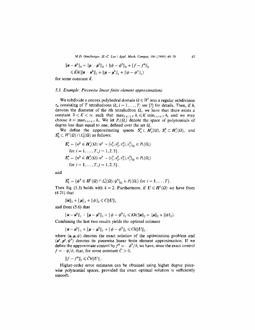
lb - 40 + lla - PhIlo + II4 - 4% + Ilf -f%l awll~ - 41, + IIP - PhII, + lid - do,)

for some constant k.

67

5.3. Example: Piecewise linear finite element approximations

We subdivide a convex polyhedral domain Q E R3 into a regular subdivision rh consisting of T tetrahedrons Sz;, i = 1, . . . : T; see [7] for details. Then, if hi denotes the diameter of the ith tetrahedron Qi, we have that there exists a constant 0 < K < oc, such that max ~~isrh,<K rniniGi<rhi and we may choose h = maxi siG T hi. We let PI (52,) denote the space of polynomials of degree less than equal to one, defined over the set Q,.

We define the approximating spaces Si c Hi(Q), $ c H:(Q), and St c H’(Q) n L;(Q) as follows:

s; = {IJ” E H&2): vh = (t&u;! vi), f&, E Pl(Qi)

for i= I,... ,ci= 1,2,3], SF = (27” E H,‘(Q): tJh = (uf, u;, lli), U,hln, E PI (Qj)

for i= l,... ,T,j= 12~31,

and

Si = {I)” E H’(Q) nLi(S2): @In, E P,(Q) for i = 1,. . . , T}.

Then Eq. (5.3) holds with k = 2. Furthermore, if U E H’(Q) we have from (4.21) that

II42 + Ilall2 + 114% G Cll~lll and from (5.6) that

lb 4I, + IIP - PhII, + II4 - 4hll, ~K~(ll42 + llPll2 + ll4lM~ Combining the last two results yields the optimal estimate

ll~-4, + lkPhlll + II@-4% ~CJ4lW,> where (u, c, tj) denotes the exact solution of the optimization problem and (I?, ph, tj’) denotes its piecewise linear finite element approximation. If we define the approximate control by fh = -4*/d, we have, since the exact control f = +/6, that, for some constant ? > 0,

Ilf -fhll, G w4l1~ Higher-order error estimates can be obtained using higher degree piece-

wise polynomial spaces, provided the exact optimal solution is sufficiently smooth.

68 M.D. Gunzburger, H.-C. Lee I Appl. Math. Cornput. 100 (1999) 49-70

6. The other optimal control problems

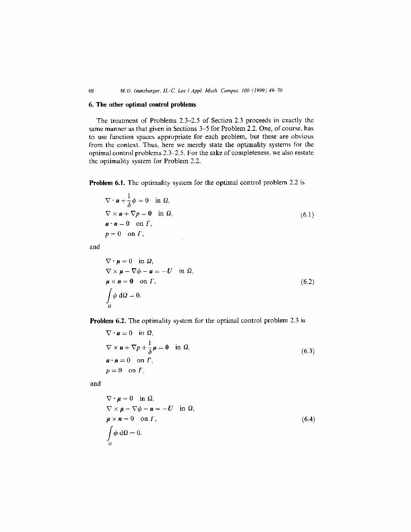
The treatment of Problems 2.3-2.5 of Section 2.3 proceeds in exactly the same manner as that given in Sections 3-5 for Problem 2.2. One, of course, has to use function spaces appropriate for each problem, but these are obvious from the context. Thus, here we merely state the optimality systems for the optimal control problems 2.3-2.5. For the sake of completeness, we also restate the optimality system for Problem 2.2.

Problem 6.1. The optimality system for the optimal control problem 2.2 is

V*u+j4=0 in Q,

Vxu+Vp=O inQ,

u-n=0 onr,

p=O onr,

and

V.jt=O ina,

Vxp-VC$--u=-U in52.

pxn=O onr:

s $dL’=O.

n

(6.1)

(f-5.2)

Problem 6.2. The optimality system for the optimal control problem 2.3 is

V-u=0 ina,

Vxu+Vp+ip=O inQ,

u-n=0 onr:

p=O onr,

and

V-p=0 in@

Vxp-V@-u=-U in52,

pxn=O onr,

(6.3)

(6.4)

M.D. Gunzburger. H.-C. Lee I Appl. Math. Comput. 100 (1999) 49-70 69

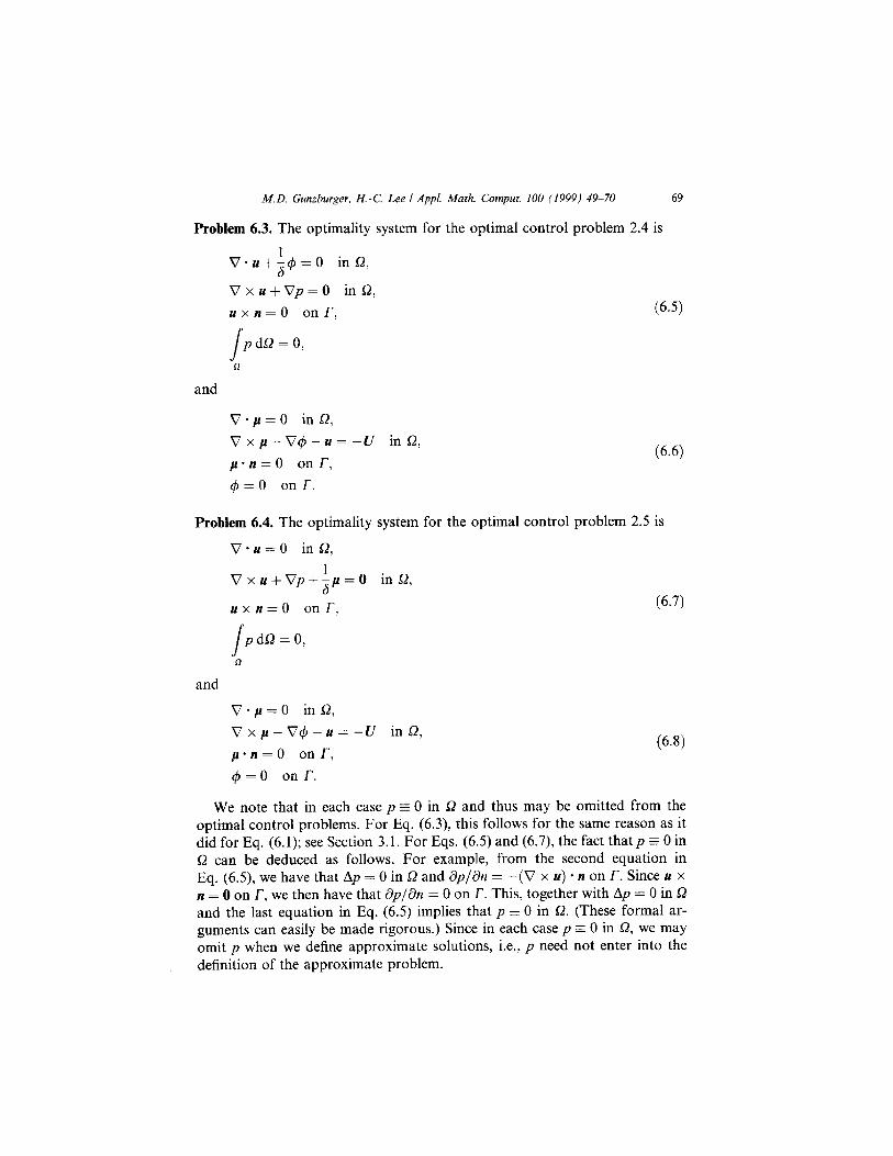
Problem 6.3. The optimality system for the optimal control problem 2.4 is

0.u+$$=O in 51,

VxufVp=Q in52,

uxn=O onr, (6.5)

s p&2=0>

n

and

V-p=0 in51,

VXa--V4-u=-U inS2,

p-n=0 onr,

d=O on r.

(6.6)

Problem 6.4. The optimality system for the optimal control problem 2.5 is

V*u=O inSZ,

Vxu+Vp+kp=O in@

uxn=O onr: (6.7)

J’ pdQ=O,

R

and

V-p=0 inn,

Vxp-V+u=-U in52,

p-n=0 onr,

4 =0 on r. (6.8)

We note that in each case p = 0 in 52 and thus may be omitted from the optimal control problems. For Eq. (6.3), this follows for the same reason as it did for Eq. (6.1); see Section 3.1. For Eqs. (6.5) and (6.7) the fact that p z 0 in R can be deduced as follows. For example, from the second equation in Eq. (6.5) we have that Ap = 0 in L? and dp/dn = -(V x u) * n on r. Since u x n = 0 on r, we then have that dp/dn = 0 on r’. This, together with Ap = 0 in 52 and the last equation in Eq. (6.5) implies that p = 0 in Q. (These formal ar- guments can easily be made rigorous.) Since in each case p E 0 in 52, we may omit p when we define approximate solutions, i.e., p need not enter into the definition of the approximate problem.

70 M.D. Gunzburger, H.-C. Lee I Appl. Math. Comput. 100 (1999) 49-70

Note that, on the other hand, C$ # 0 in general. In fact, in order for 4 z 0 in 52 we need V - U = 0 in 52 for (6.5), (6.6), and (6.7), (6.8) and, for (6.1), (6.2) and (6.3), (6.4), we need V * U = 0 in 12 and U - n = 0 on T. If these conditions on U hold, then the optimal control problems have the trivial solution II E 0 in Q, i.e., the problems are uninteresting.

References

[1] R. Adams, Sobolev Spaces, Academic Press, New York, 1975. [2] S. Agmon, A. Doughs, L. Nirenberg, Estimates near the boundary for solution of elliptic

partial differential equations satisfing general boundary conditions II, Comm. Pure Appl. Math. 17 (1964) 35-92.

[3] Y. Roitberg, A theorem about the complete set of isomorphisms for systems elliptic in the sense of Douglis and Nirenberg, Ukrain. Mat. Zh. 27 (1975) 447450.

[4] C. Chang, M. Gunzburger, A finite element method for first order elliptic systems in three dimensions, Appl. Math. Comp. 23 (1987) 171-184.

[5] E. Zeidler, Nonlinear Analysis and its Applications, vol. III, Springer, New York, 1988. (61 K. Yosida, Functional Analysis, Springer, Berlin, 1965. [7] P. Ciarlet, The Finite Element Method for Elliptic Problems, North-Holland, Amsterdam,

1978.