Analysis #and adaptive modeling of highly heterogeneous

ELSEVIER

Computer methods in applied

mechanics and englneerlng

Comput. Methods Appl. Mech. Engrg. 148 (1997) 367-391

Analysis #and adaptive modeling of highly heterogeneous elastic structures

J. Tinsley Oden”*, Tarek I. Zohdi*, Texas Institute “For Computational and Applied Mathematics, The Universi& of Texas at Austin, Austin. 7X 78712. USA

Received 6 December 1996; revised 7 February 1997

Abstract

In this paper, we develop a theory and methodology for obtaining approximate solutions to boundary value problems describing the

deformation of highly heterogeneous linearly-elastic structures. The method, which represents a significant departure from traditional

homogenization methods, provides a systematic and rigorous approach towards resolving the effects of microstructure of different scales on

the macroscopic response of complex heterogeneous structures. An early variant of this method was first introduced in [IO]. The method,

referred to as HDPM (Homogenized Dirichlet Projection Method), proceeds by first solving an auxiliary homogenized boundary value

problem, describing the deformation of a structure with the same exterior geometry, but with a selected set of uniform material properties.

The adequacy of this homogenized solution is then determined using an a posteriori error estimate that provides a measure of the error of the

homogenized solution in subdomains of the structure compared to the solution of the fine-scale heterogeneous problem, without specific

knowledge of this fine-scale solution. In those subdomains where the homogenized solution is deemed acceptable, it is retained. However, in

subdomains where the homogenized solution is inadequate, as is determined when the estimated error exceeds a preset tolerance, a local

boundary value problem is constructed by projecting the homogenized displacements onto a partition designed to isolate these subdomains.

These local boundary value problems are then solved in those subdomains where the homogenized solution is inaccurate using the exact

microstructure with the approximate local boundary conditions. A posteriori error estimates are made to ascertain the quality of the resulting

solution. If the quality of the solution remains inadequate, above a preset error tolerance, a two stage adaptive procedure is implemented.

Stage-I (‘material adaptivity’) corresponds to modifying the homogenized structure’s material properties. If, after Stage I, the solution

quality is still inadequate, the subdomains of local solution are enlarged, thereby modeling in greater detail the actual microstructure, and the

local solution process is. repeated (Stage-II, ‘subdomain unrefinement’). The main feature of this method is that only in subdomains where

the error in the usual homogenized solution is above a preset tolerance is the microstructure taken into account. The cost of this method is

shown to be orders of magnitude cheaper than direct huge-scale computational simulations of micromechanical events. The results of several

numerical experiments are provided to demonstrate the method and verify theoretical estimates.

1. Introduction

In this work, we present a method for the solution of boundary value problems modeling the deformation of

structures composed of highly heterogeneous linearly-elastic materials. We concentrate on materials formed by a homogeneous matrix embedded with particulate matter of different properties (Fig. 1). However, the results presented are not limited to materials of this type, and can, in theory, be used for materials with virtually any

microstructure. A straightforward calculation reveals that an accurate numerical approximation of fine-scale solutions of

* Corresponding author.

’ Director of TICAM, Cockrell Family Regents Chair in Engineering #2.

2 Research Assistant and CAM Fellow.

0045-7825 /97/$17.00 0 1997 Elsevier Science S.A. All rights reserved

PII SOO45-7825(97)00032-7

368 J.T. Oden, T.I. Zohdi I Comput. Methods Appl. Mech. Engrg. 148 (1997) 367-391

E ijkl

I x

Fig. 1. A general particulate composite body.

problems involving relatively simple, dilute microstructural features by, say, finite element methods, may

require huge memory capacities and the solution of problems sizes exceeding those of all available supercomputers. A new and more systematic approach is needed to cope with these types of analyses. In our

view, the key to the resolution of such problems is the development of rigorous a posteriori estimates of the error in various homogenized approximate solutions and the implementation of an adaptive modeling process that permits one to use only enough fine-scale information to deliver an answer of a preset accuracy, and no more. This is the philosophy behind the approach developed here. Such a process leads to a characterization of the material coefficients in boundary-value problems simulating the behavior of heterogeneous structures that does not only depend upon the local microstructure but also depends upon the data: the loads, geometry, and boundary conditions of the specific problem at hand.

The method developed here involves the decomposition of boundary value problems of this class into sets of

smaller decoupled problems. In this method, the boundary-value problem, with the original boundary conditions and loading, is solved with a uniform, regularized approximation of the exact material properties, so-called homogenized properties. This is a relatively inexpensive operation since the fine-scale features are eliminated.

The displacements are then projected from this homogenized solution onto a preselected partition of the domain. This partition, along with the displacement data prescribed on the partition boundary, forms a set of smaller independent subdomain problems. These local boundary value problems are then solved in regions where the homogenized solution is deemed inaccurate using the exact microstructure with the approximate local boundary conditions. It is important to emphasize that the approximate local boundary conditions may be highly nonuniform due to the external loading and external geometry. We refer to this method as the HDPM- Homogenized Dirichlet Projection Method.

Certainly, there is error introduced by approximating the local boundary data. Furthermore, the quality of the solutions produced by this process is extremely sensitive to the choice of the homogenized material properties used in the construction of the local boundary conditions. Consequently, it is very important to determine an optimal or near optimal set of homogenized properties, which minimize this error. The term ‘optimal’ implies

J.T. Oden, T.I. Zohdi I Comput. Methods Appl. Mech. Engrg. 148 (1997) 367-391 369

that the HDPM solution is designed to be as close as possible (for a certain partition) to the exact microstructural solution in an energy norm. The optimal choices of homogenized properties are shown to be those which generate microstructural solutions which minimize a certain augmented elastic potential. To check

the resulting answers, sharp upper bounds on the error inherent in the method are developed. If the estimated error is intolerable, .the partition is changed, i.e. the subdomains are increased in size, and correspondingly new optimal materials are sought. The final result of this process is the determination of a relatively inexpensive and

accurate approximation to the microstructural field variables, the HDPM solution, which can then be used in a

subsequent structural analysis. Following standard practice in the mechanics of composite materials, we assume throughout this study that

the exact topology and mechanical properties of the microstructure are a priori known exactly. We plan to discuss how this assumption can be removed using tomographic techniques in a later work. After this introduction, we present the ‘exact’ or so-called ‘fine-scale’ problem formulation, which is a characterization of the linear elasticity problem with elasticity tensor E that is highly oscillatory for the fine-scale problem. The ‘homogenized problem’ involves a boundary-value problem in which E is replaced by an average or homogenized elasticity tensor E”. This is discussed in Section 3 of the paper. Since regularity of the solutions is a critical issue for problems with microstructure, and therefore internal material interfaces, we consider a weak

formulation of the boundary value problems of elasticity to admit generalized solutions. In Section 4, we record a posteriori error estimates providing bounds in a fine-scale energy norm of the difference between the fine-scale

and the homogenized solutions. In Section 5 we focus on constructing perturbations of the homogenized solutions on subdomains via HDPM. In Section 6 we prove several fundamental theorems giving estimates of

the error between the perturbed (HDPM) solution and the ‘exact’ solution. We confirm these estimates with numerical experiments in three dimensions. The overall adaptive algorithm is presented in Section 7. We also discuss the implementation of the HDPM here. Afterwards, we present some relevant numerical experiments on examples of materials containing uniformly distributed particulates. Finally, we end the study with several concluding comments, including observations on the relationship of the HDPM and classical ideas on Representative Volume Elements (RVEs). Additional important information is included in Appendices A-D.

2. The exact problem

We model a complex heterogeneous structure as a linearly-elastic solid in static equilibrium under the action

of body forces f and surface tractions t. Despite its fine-scale microstructure, the body is assumed to have a precisely polished exterior surface, allowing the consideration of smooth domain boundaries in the corresponding mathematical model. The body occupies an open bounded domain in 0 E [WN and its boundary is denoted aa. The boundary dfl consists of a portion 4 on which the displacements are prescribed and a part 4 on which tractions are prescribed, 80 =c U I;, I: fl I; = 8.

Let H’(a) denote the usual space of functions with generalized partial derivatives of order ~1 in L*(O)

defined on an open domain 0 E lQN; N = 1, 2 or 3. We define H’(~)d~f[H’(~)]N as the space of vector-valued

functions whose components are in H’(O), and we denote L’(O) dzf[‘[L2(&!)]N. Accordingly, the corresponding norms are

(1)

where ui are Cartesian components of u. The data are assumed to be such thatf E L2(@ and t EL*(J), but less smooth data can be considered without complications.

The space of admissible displacement, V(G), consists of those displacement fields in H’(a) which satisfy homogeneous (displacement) boundary conditions on c,

v(n)Ef{v E&(a): Ulr. = 0). (2)

The displacements on 4 are prescribed as follows: 3 ti E H’(O); ulr. = u^ Ir,. li is specified displacement data

on c. Thus, the actual displacements of the body are in the translation {G} + V(a).

370 J.T. Oden. T.I. Zohdi I Cornput. Methods Appl. Mech. Engrg. 148 (1997) 367-391

We consider the classical principle of virtual work characterized by the following variational boundary-value problem of elastostatics:

(3)

where

92(11, u)zf Vu : EVu dx , s

t . v ds , I;

and where Vu : Vu dgftr[(Vv)TVU] = Cyj=, auj/axi au,/&, are generalized partial derivatives of ui and ui, 1 s i,

j S 3. Throughout this work we shall use the symbol ‘via0 for boundary values of v E H’(0), in the sense of traces. In the absence of regularity sufficient to guarantee integrability, the symbol J will also denote duality

pairing in the appropriate spaces.

The mechanical properties of the material are characterized by the elasticity tensor E which is assumed to be a given bounded function in RN XN satisfying the following symmetry and ellipticity conditions

3a,,cw,>O a;A:A~A:E(x)A~qA:A VAE [WNxN, A=AT,

Ejjk,(x) = Eli&) = E+(X) = Ek,,j(x) 1 S i, j, k, 1 C N , (5)

E,,,,(x) being the Cartesian components of E at a.e. point x. The difficulty in solving this problem is due to, again, the highly oscillatory coefficient tensor E which must characterize the highly heterogeneous micro-

structure possibly varying widely, and frequently in complex non-periodic ways in the domain 0.

We note that if the data in (3) are smooth and if (3) possesses a solution u that is sufficiently regular, then u is the solution of the classical linear elastostatics problem,

-V . (E(x)Vu(x)) =f(x) x E R

u(x) = G(x) x E r,

(EVu(x)) . n = t(x) x E I;.

(6)

3. The homogenized problem

The use of a regularized approximation to E, denoted E”, leads to a new more tractable problem, which we refer to as the homogenized problem,

Find u” E {ti} + V(0) such that

.BO(uO, v) = P(v) v v E V(0) (7)

where

93 O(uO, v) fzf Vu : E”Vuo dx , 9-(v>d~f I

f.v dX + I

t . v ds , R r,

(8)

where E” E RN2xN2 satisfies conditions of symmetry and ellipticity

LY;,cY~>O CY~A:AAA:E~A~~~A:A VAE[WNxN, A=AT

E;,,= ’ ’ ’ ’ ’ k,lsN. (9)

E,,, = Eijrk = Ekr;,. 1 5 I, J,

The boundary conditions are identical to those of the exact (heterogeneous elasticity) problem. Under the adopted conditions, both (3) and (7) possess unique solutions u, u” E {ti} + V(n), respectively.


In order to judge the quality of a homogenized solution, it is important to adopt a measure of error with the

properties of a norm. We choose the energy norm of the difference of the homogenized and exact solutions as a measure of the quality of the homogenized solution

REMARK 3.1. At this point, we emphasize that E” is only some type of regularization of E and that there is no

restriction on the anisotropy of E ‘. E” may be highly anisotropic even if E is isotropic. However, for particulate composites, E” is often assumed to be macroscopically isotropic because of a lack of directional dependence of the macroscopic material properties resulting from combinations of isotropic particulate constituents.

REMARK 3.2. Traditionally, a so-called ‘effective’ material property, E”, is used in engineering analysis instead of the highly nonuniform microstructural properties, characterized by E. This tensor is usually an

approximation of the relation between averages, defined by

(a) = E*(E) u = EE Q = (VU + (VU)~)/~, (11)

where ( - ) = (1 /IL!\) J,, * dx. In general, E* is not a material property, i.e. it depends on the microstructure.

4. An upper bound on the homogenization error

Clearly, the solution u” is in error. A first goal is to determine the error without calculating II, and, therefore,

we must seek some way of estimating [(u - u”llE(on). We record the following important result.

THEOREM 4.1. Let u be the exact solution to (3). Then, with the previous dejinitions in force

I Ilu - uOll ,I,,,~~~l,aoVuoll~E,,,,~f~ 90=Z-E-‘Eo ( (12)

where explicitly

PROOF. See [lo]. Cl

(13)

This estimate is ‘sharp’ in the sense that it collapses to an equality in many special cases, including the cases of uniform exterior loading. Numerical experiments indicate that the estimate provides an excellent estimate of

the error in the homogenized solution. For details see [lo] and Appendix A.

5. Construction of an approximate microscopic field-through HDPM

In general, the homogenized solution u” can be a very poor approximation to the fine-scale solution II. To obtain an improved solution, we project the macroscopic homogenized solution onto a preselected partition of the domain which forms a set of smaller decoupled nonoverlapping subdomains covering the body (Fig. 2). Thereafter, we solve local boundary value problems posed over the subdomains using the exact microstructure, but with boundary data supplied by the homogenized solution, where needed. The advantages of such a method, if it is proven accurate, should be clear

l it results in a dramatic reduction in memory requirements, since only local subdomain information needs to be stored and can subsequently be overwritten repeatedly throughout the computational process,


Fig. 2. An example of global/local decomposition.

l it results in a massive reduction of total operation counts over a direct formulation, since only local problems are solved, and

l it admits to parallel implementation, since the local problems are decoupled. With these benefits in mind we proceed to lay down a general framework for the method.

5.1. Construction of local subdomain problems

We consider a general curvilinear, non-convex domain, 0, and we introduce a bounding box (Fig. 3) iI*, as an open rectangular parallelepiped of minimum volume such that it encloses the entire material body, and that each domain remains simply connected and Lipschitz:

diaO* = inf dia{O : fi C 0) . (14)

The subsequent partition can be achieved by partitioning the bounding box and calculating the intersection between elements of the bounding box partition and the domain. For example, we can define a partition 22

through sub-boxes, 0, by

LJ:=, q ,=O. q ,nCl,=fI, KZL, 1~K,L~N(i2n),

Subdomains

Bounding Box

(15)

Fig. 3. The nomenclature for the construction of a general partition for an HDPM analysis.


where each Cl, is of equal size. We define the local subdomain 0:: C fi as

0(-Q=@, U;:,“‘s;=n, @i-30,0=0, KZL. (16)

We define the boundary of an individual subdomain @i, as a@: consisting of a portion rKU where the

displacements are prescribed and a part r,, where tractions are prescribed

r,, %fao,"\rK, fK,%faoF nr;. (17)

We define the following local function spaces

V(O~)~f{vEV(f2),u=0 on a\O~,u~,U=O}. (18)

Let gKK, 1 SK C FJ( 22 q ), denote the extension operator from V(OF) into V(0) that identifies each u, E V(@) with a function u in V(f2) such that

42,s:: = 0. (19)

8 extends the domain of definition of a locally defined function to the entire domain. We define

U;d~fUOlop EH’(O,O). GO)

We denote by tii the function that is zero outside of 0: and that is equal to the solution to the following local

variational boundary-value problem of elastostatics,

Find zZ~ E {no,} + V(@) such that

%&? UK) = S&UK) v u, E V(@)

where lSK<N=N(gO) and

(21)

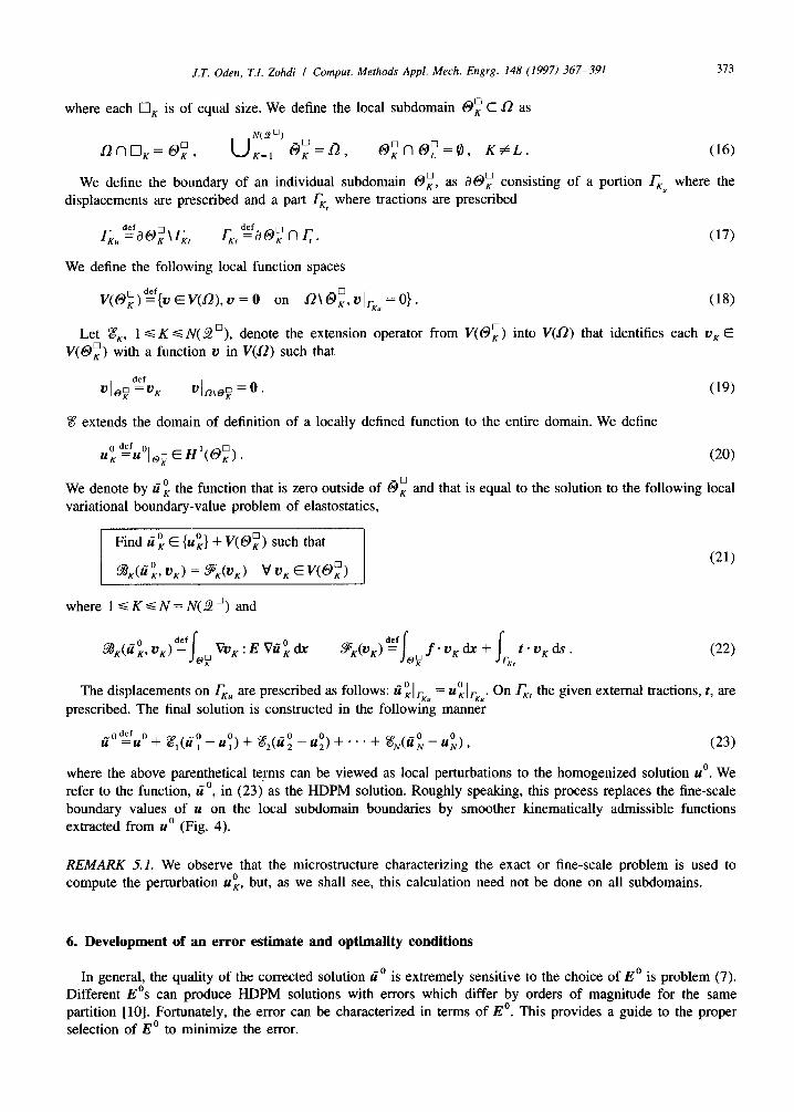
The displacements on r,, are prescribed as follows: zZ~I~~, = u:[~~.. On I& the given external tractions, t, are prescribed. The final solution is constructed in the following manner

_odef o u. =z4. + qlii;-u;)+ qa;-U;)+“.+ q&z;-u;,, (23)

where the above parenthetical te,rms can be viewed as local perturbations to the homogenized solution u’. We refer to the function, tie, in (23) as the HDPM solution. Roughly speaking, this process replaces the fine-scale

boundary values of u on the local subdomain boundaries by smoother kinematically admissible functions extracted from u” (Fig. 4).

REMARK 5.1. We observe that the microstructure characterizing the exact or fine-scale problem is used to compute the perturbation u;, but, as we shall see, this calculation need not be done on all subdomains.

6. Development of an error estimate and optimality conditions

In general, the quality of the corrected solution zZ” is extremely sensitive to the choice of E” is problem (7). Different E’s can produce HDPM solutions with errors which differ by orders of magnitude for the same partition [lo]. Fortunately, the error can be characterized in terms of E”. This provides a guide to the proper selection of E” to minimize the error.

374 J.T. Odett, T.I. Zohdi I Comput. Methods Appl. Mech. Engrg. 148 (1997) 367-391

ACTUAL LOCAL BOUNDARY CONDITIONS HDPM LOCAL BOUNDARY CONDITIONS

Fig. 4. A pictorial representation of an HDPM construction of local boundary conditions.

6.1. Error estimates based on elastic potentials

We begin by first recording a classical result, which we use repeatedly, the Principle

Energy: Let u be the exact solution to (3). Then, with the previous definitions

F(U)d.qU*) vu*E{ti}+v(n>

where

Y(IV)zf; B(w, w) - 9(w) w E {ti} + V(O) .

The following result guarantees that the solution produced by the localization process more accurate solution, regardless of the choice of E”.

THEOREM 6.1. Let u be the exact solution lo (3). Then, with the previous dejkitions

_J

which directly implies

of Minimum Potential

(24)

(25)

will always provide a

in force

(26)

(27)

PROOF. Since each tii is solution to the local boundary value problem governed by (21), then, by the Principle of Minimum Potential Energy, each tii minimizes the local potential energy function FK, where

V WK E {U”,} + V(@>, l<KCN(9). (28)


Clearly, from the construction of the global function in (23),

N( 2 ) N( 9 )

Y(u”) = c S,(u”,) 2 x 5-&l”,) = Y(tiO) . K=l K=l

Therefore,

qtiO> - Y(U) :s Y(U”) - Y(U) .

Let w be an arbitrary element, such that w E {ri} + V(a). It can be easily shown that

IIW - r&J, = Z!Y(w) - 29(U)

which, in view of (3 1) completes the proof. 0

(29)

(30)

(31)

In passing we note that directly from (3 l), the distance between the potential of tie and its modeling error, measured in the energy norm, is independent of the homogenized properties used

Y(zZO> -; IJU .- iZ”&j, = Y(U). (32)

We now characterize the expression for the error exactly, in terms of the homogenized solution u” as a function of E”, denoted u”(Eo).

THEOREM 6.2. Let u be the exact solution to (3) and

v*(Evtio,). fEH-‘(Of)

(E vti”,,*n ‘EH-“2(rK,\IJ.

Then, the following holds

(33)

lb - ~“ll~(o, = (EVti;)~n,+&u)ds. (34)

PROOF. For any admissible virtual displacement u E V(O), we have from the principle of virtual work

(f+V.(EVu”O,))4.x

(t-EVz+n,)ds-

Hence, with v = II -- u^’ EV(Q

(35)

(36)

and, therefore, since: 1’ = u” on r,,, \r,


(37)

The right-hand side of (34) can be interpreted as the work done by the jumps in traction moving through the difference between the actual and homogenized displacement on interior local subdomain boundaries.

6.2. Error in terms of an augmented potential difSerence

Clearly, the right-hand side of (34) is what we seek to minimize when choosing a homogenized property for a HDPM analysis to reduce the modeling error. Importantly, the quality of the solutions produced by this process

is extremely sensitive to the choice of the homogenized material properties used in the construction of the local boundary conditions. For more details see [lo]. The choice of the ‘optimal’ homogenized material, denoted E ‘,‘, that which admits a minimal error in the energy norm, can be directly obtained by locating the minimizer ZZ ‘(E”+) of the following

(38)

This expression follows directly from (26) and (34). The quantity is thus seen to be an augmented elastic

potential. Therefore, an optimal homogenized material choice for HDPM is one that satisfies (for a certain partition)

JII(E”“) = inf,L(R)1N2X,+ M(E”) J%(E~)~~~(~Z~(E~)). (39)

Of course, we require E” to remain elliptic. Since Y(U) is independent of u’, and subsequently E”, if we

minimize Y(zi’), we minimize the error. Clearly, an optimal E” may not be unique and is dependent on the external loads, geometry, microstructure and the partition used. We may use this potential to characterize the error inherent in HDPM. However, two preliminary results are needed beforehand. First, we note that

9-(U”) = Y(U) + ; ))U - U”l];<n, G Y(U) + ; c* (40)

where this result is obtained by directly applying (31) to the macroscopic homogenized solution. Second, by

subtracting (38) from (40) and using (34) we obtain

9-(ZiO) - quo) = ; llzzO - ull;(~) - [Ill0 - ull:,n) .

These preliminaries lead us to the following key result:

(41)

COROLLARY 6.1. Let II be the exact solution to (3). Then, if (33) holds,

pi

where @‘(Go, u”, l)dzf2( ,7(ti”) - y(u’)) + 5’.

PROOF. This follows directly from (40) and (41). 0

(42)

Note that, if the homogenized error estimate (5) is exact, the inequality in (42) becomes an equality. The quality of the error estimate hinges on the proximity of 5 to J]u - ~~~~~~~~ which is usually extremely close (see Appendix A and [IO]).


6.3. A local solution sensitivity property

COROLLARY 6.2. Under the previous de$nitions and hypotheses, for K = 1,2 , . . . , N( 9 >,

rzi (43)

PROOF. This follows directly from (3 1) and by applying Theorem 4.1 locally to an individual subdomain (21),

K= 1,2.. .N(9). 0

The expression bounded in (43) is the local sensitivity of the structure to a change in its material properties.

Notice in subdomains where L& is small, there is little predicted difference in the homogenized solution and perturbed solution in the energy norm. Therefore, there exists the ability of selecting only ihose subdomains with

&‘s above a certain tolerance for the local solution process.

7. The overall adaptive algorithm

An HDPM analysis is as follows:

Step 1: Initialization. Given the domain, the data E, ti, f, t, Q 4 and c, construct a partition 9 = {O,}f=, , and determine an initial homogenized material tensor E ‘. One may use an approximation to the relation between

the averaged tensor ( 11) as a first guess for E”. Specify local sensitivity and global error tolerances, q and a;,

respectively (ultimately, ~IIu~II~~+~, X lO~l/l.~l zf( &),,, and ~+~ll,o,~, EfetO,).

Step 2. Using E”, solve the homogenized problem and obtain u”.

Step 3. Compute the local sensitivities

~~ti;-~;~~~~~~~~~J~ K=l,2...N(s). (44)

Step 4. Use u” as boundary conditions on the interior interfaces of the partition. Solve only local subdomain prob&ms that are above a prespecified sensitivity tolerance, which we denote as members of the index set

9ta,,, = {K E $,,,v & ’ (&),,J V K E $t,,,

and T,,(E Vfii).n =t on r,

Step 5. Form the: following global ‘perturbed’ function

-0 U =u”+ 1: 6_T&-z4”,).

=.~,,I (45)

Step 6. Compute the estimated error in the perturbed solution

f&tiO, u”, [) %[2( Y(tiO) - ($(zJO)) + [*I l’* . (46)

Step 7. If $(a’, u”, 5) s &, = a;l~~~~~,~~,, STOP. If #(/(ho, u”, f) > &,, then change the homogenized


material properties and repeat Steps 2-7. A method for the determination of improved homogenized material properties is given in Appendix D. If the error is not met with this partition with the ‘optimal’ Eo3*, then go to Step 8.

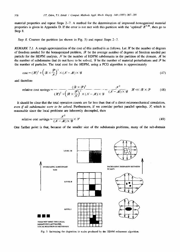
Step 8. Coarsen the partition (as shown in Fig. 5) and repeat Steps 2-7.

REMARK 7.2. A rough approximation of the cost of this method is as follows. Let X be the number of degrees of freedom needed for the homogenized problem, %! be the average number of degrees of freedom needed per

particle for the HDPM analysis, X be the number of HDPM subdomains in the partition of the domain, JB be

the number of subdomains that do not have to be solved, Ce be the number of material perturbations and 9 be the number of particles. The total cost for the HDPM, using a PCG algorithm is approximately

cost==(X)2+(~x~)2X(X-~)X 9

and therefore

(47)

relative cost savings = (92 x sy

(I)2+~i2x%)2x(r_~)~~~(~-~)x~ 3Y<c9xx (48)

It should be clear that the total operation counts are far less than that of a direct micromechanical simulation,

even if all subdomains were to be solved. Furthermore, if we consider perfect parallel speedup, 9, which is reasonable since the local problems are inherently decoupled, then

x2 relative cost savings = (x _ &) X 9 X Y (49)

One further point is that, because of the smaller size of the subdomain problems, many of the sub-domain

LEVEL 111

t

INCREASING SUBDOMAIN

SLZE

LEVEL II

LEVEL I

DOES NOT MEET THE LOCAL SENSITIVITY ESTIMATE!% LOCAL SOLUTlON IS NECESSARY

INCREASING DISPARITY BETWEEN SCALES

I

Fig. 5. Increasing the disparities in scales produced by the HDPM refinement algorithm.


operations are cache-optical, thus making the operations ideal for most modern computer architectures (such as

RISC).

REMARK 7.2. The sensitivity tolerance parameter a1 can be selected somewhat arbitrarily, simply as a percentage of the global homogenized energy density, or from an eigenvalue calculation [ 111.

REMARK 7.3. Many variations of this algorithm are possible, including adaptive steps which automatically

generate appropriate partitions to begin the HDPM.

8. Numerical experiments

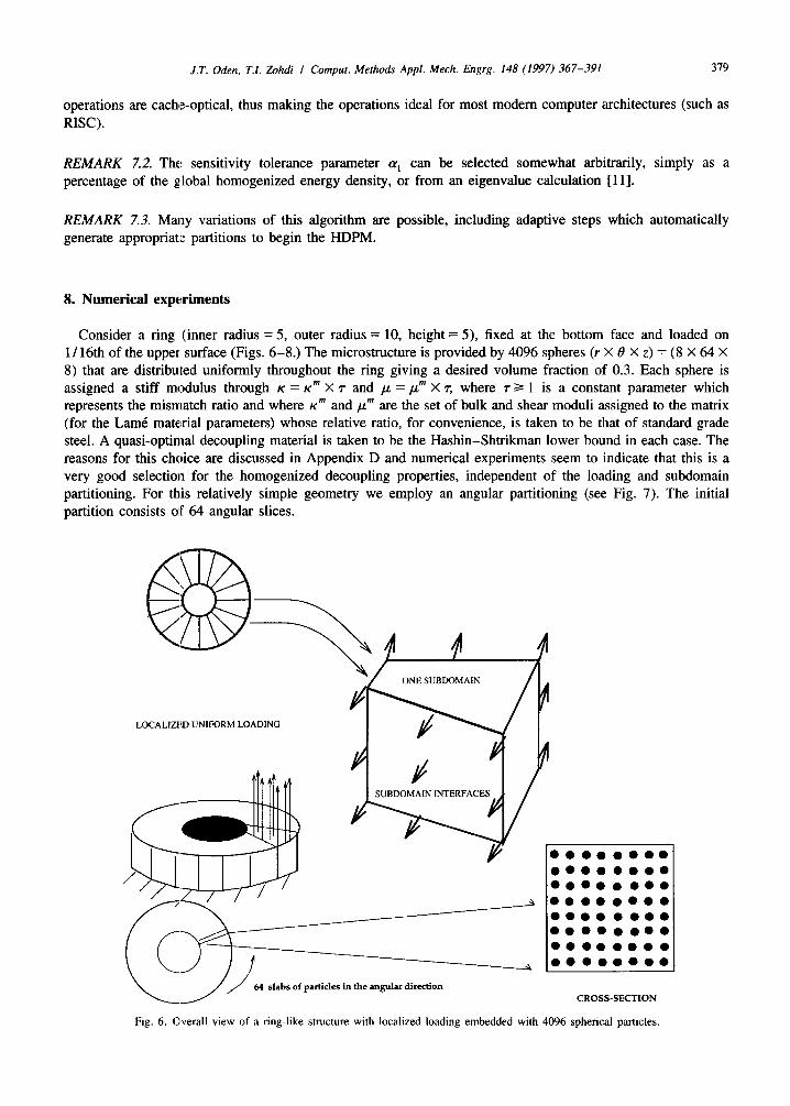
Consider a ring (inner radius = 5, outer radius = 10, height = 5), fixed at the bottom face and loaded on

1 / 16th of the upper surface (Figs. 6-8.) The microstructure is provided by 4096 spheres (r X 8 X z) = (8 X 64 X 8) that are distributed uniformly throughout the ring giving a desired volume fraction of 0.3. Each sphere is

assigned a stiff modulus through K = K~ X r and p = $’ X r, where r 2 1 is a constant parameter which represents the mismatch ratio and where K~ and r(~‘” are the set of bulk and shear moduli assigned to the matrix (for the Lame material parameters) whose relative ratio, for convenience, is taken to be that of standard grade

steel. A quasi-optimal decoupling material is taken to be the Hashin-Shtrikman lower bound in each case. The reasons for this choice are discussed in Appendix D and numerical experiments seem to indicate that this is a very good selection for the homogenized decoupling properties, independent of the loading and subdomain partitioning. For this relatively simple geometry we employ an angular partitioning (see Fig. 7). The initial

partition consists of 64 angular slices.

NE SUBDOMAIN

LOCALIZED UNIFORM LOADING

BDOMAIN INTERFACES

slabs of particles in the angular direction CROSS-SECTION

Fig. 6. ONvera view of a ring-like structure with localized loading embedded with 4096 spherical particles.


Fig. 7. The actual ring microstructure with 4096 embedded spheres in a homogeneous matrix ( VS = 0.3) and the initial subdomain

partitioning.

In these tests we also compare two parameters which reflect the distortional energy content locally in the body, /3” and p”:’

i = 1,2, . . . , No = number of homogenized finite elements (51)

tr 6~’ where co’ = l o - - 3 I and

,g” = number of homogenized finite elements (52)

where E’ = Q - (tr l )/31 and where w is the volume of the appropriate finite element. These parameters provide some practical insight into the differences that may be observed between the purely homogenized structure and

’ We recall the distortion energy failure criteria is

c’ :Ea'z %

where V is a constant experimentally determined constant from a simple shear or tension test.


Fig. 8. Final heterogeneous structure produced by HDPM for an elastic ring composed of 4096 spherical inclusions in a homogeneous

matrix; the HDPM is applied initially to a partition of 64 subdomains, each with 64 inclusions, with an applied uniform load over 4

subdomains. HDPM yields a solution that differs an estimated 7.4-8.88 from the fine-scale solution in the normalized energy norm

(llu - QOll,W, = 0.074(lu011,ao,) with mismatches ranging from lo-100 for 64 subdomains, estimated 5.1-X3% for 32 subdomains (loaded

over 2 subdomains) and estimated 4.0-4.38 for 16 suhdomains (loaded over 1 subdomain).

that obtained if the microstructure is taken into account through the HDPM. In the following experiments

(&‘,>,O, = o.511~“ll,(~, x l@,“lwl. By comparing the values of 4’ and I) in Table 1, it is seen that the HDPM can reduce the error inherent in

using a homogenized solution dramatically. For this problem, 15.5 C lHl# C 88.6, depending on the mismatch and subdomain partitioning. In all numerical calculations, sufficiently fine meshes were taken to insure

Table 1

Global Energy Mdepsures: Local tensile loading E;ver 1/16th of the top surface, ?W = 0.3,dcf3 dGrnumber of spheres, S dzrnumber of

subdomains, B/S = spheres per subdomain, LSS =number of local subdomains solved. ROC =ratio of a direct simulation’s operation

counts (if it were possible) to the HDPM simulation’s operation counts. The Hashin-Shtrikman lower bound is used in all cases.

7 B/S S B”‘” x 10-s p”.” x 10-S LSS ROC

10 64 64 1.15 0.074 192.36 5.41 14 293 50 64 64 2.69 0.084 140.79 4.91 16 256

100 64 64 3.81 0.088 102.10 4.85 16 256 10 128 32 1.15 0.051 423.51 5.41 6 171 50 128 32 2.69 0.056 184.05 4.91 8 128

100 128 32 3.81 0.058 168.46 4.85 8 128 10 256 16 1.15 0.040 423.59 5.41 3 85 50 256 16 2.69 0.042 175.70 4.91 3 85

100 256 16 3.81 0.043 164.50 4.85 5 51

382 J.T. Oderz, T.I. Zohdi I Comput. Methods Appl. Mech. Ettgrg. 148 (1997) 367-391

0 0 10 20 St%omain 40 50 60

Number

Fig. 9. The normalized local sensitivity indicators I&/(&),,,, normalized for each r individually, r = 10, 50 and 100, as a function of

subdomains (64 subdomains). The loading is in the middle, over 4 subdomains. Since for each partitioning, the subdomains are

geometrically similar (&),,, I( &),,, = constant for given z For r = 10, (&),,,,I( &),,, = 0.0134, for r = 50, (&),,,I(&),,, = 0.00576 and

for 7 = 100, (i,),,, /( I$),,, = 0.00405.

reasonable numerical accuracy. However, we note that the influence of numerical error on the modeling error

can be significant; this is discussed in Appendix C and in more detail in [l l]P The error measures are normalized according to the homogenized energy’s content, which, since it stems from a global calculation, does not change with subdomain partitioning. While this normalization is not ideal, it is a good choice due to the fact

that the number of degrees of freedom needed to determine /r&n, with sufficient accuracy practically renders

this incalculable5. To insure the accuracy of the presented results, the homogenized problem was solved with a trilinear finite element model consisting of 93,312 degrees of freedom, and every local subdomain problem

solved was solved with 50,412 degrees of freedom for the 64 subdomain case, 93,639 degrees of freedom for the 32 subdomain case, and 194,481 degrees of freedom for the 16 subdomain case. For this problem, for comparable numerical accuracy, a direct simulation was estimated to require approximately 2,765,952 degrees

of freedom.

From Table 1 it is clear that not all subdomains need to be solved, and that in approximately 3/4th of the structure the homogenized solution is adequate. As expected, this is slightly sensitive to the mismatch ratio;

however, this effect is not too pronounced, only increasing the number of subdomains to be solved by two at most. Figs. 9-l 1 illustrate that the decay of the local sensitivities is essentially insensitive to the mismatch ratio

and subdomain partitioning. It is also observed that the differences in the prediction of the local distortional strain energy content by the

homogenized and HDPM solutions are dramatically different, with the homogenized problem often producing local energy densities 30 times smaller than that of the fine-scale solutions. If one assumes that the local energy

of distortion is an adequate criteria for metal-matrix composites, the consequences of relying on the homogenized solution values can thus be catastrophic.

9. Final comments

In this work, an adaptive process is developed that designs a homogenized solution to supply nonuniform displacement data on a partition of a structure under analysis. This partition forms the boundaries of local boundary value problems posed over nonintersecting subdomains which cover the entire body. In the solution to

4 Further numerical experiments can be found in a forthcoming paper [8].

5 The solver used, discussed in Appendix B, is of the preconditioned conjugate gradient type, where the homogenized solution is used to

precondition the local solves in the HDPM.


Fig. 10. The normalized local sensitivity indicators &J(J&),,~, normalized for each T individually, T = 10, 50 and 100, as a function of subdomains (32 subdomains). The loading is in the middle, over 2 subdomains. Since for each partitioning, the subdomains are

geometrically similar (&),,, I( &;O,., = constant for given r. For r = 10, ( &)ro,I( &),_ = 0.0206, for T = 50, ( &)ro,l( L),,, = 0.0112 and

for T = 100, (&),,,I( &),,. = 0.0062.

” 2 4 6 Sub&m& Number

10 12 14 I

Fig. 11. The normalized local sensitivity indicators &./( &),,,_, normalized for each r individually, r = 10, 50 and 100, as a function of

subdomains (16 subdomains). The loading is in the middle, over 1 subdomain. Since for each partitioning, the subdomains are geometrically

similar (L),,J(L),., = Iconstant for a given r, For r = 10, (s&),,! I( &‘,),,, = 0.0295, for r = 50, (&),,, /( &;O,,,_ = 0.00127 and for T = 100,

(!L),,,N&),,, = 0.OOg9.

the local boundary value problems, the exact microstructural properties are used. By design, these boundary value problems are completely decoupled from one another, making the overall solution process well suited for parallel computation. However, the strength of the approach is that micromechanical simulations are not needed

everywhere throughout the structure. The consolidation of the local solutions where needed, along with the

homogenized solution, where it is adequate, forms an approximate microstructural solution field. In summary, we have presented

l a procedure that provides a sharp estimate of the error in the energy norm produced by homogenization procedures commonly used in engineering analysis of composites and heterogeneous materials,

l a systematic process for delivering results with a preset level of accuracy for general boundary conditions, loads geometrical shapes, and elastic properties,

l a theory and methods to resolve classical problems of multiple scales of material constituents and determine how these interact to affect the stress, displacement, and energy of elastic bodies,


l and a correspondingly better ability to predict damage in elastic materials. In general, there are cases in which all subdomains need to be solved (see [lo] for examples). In these cases

the local sensitivity is above a sensitivity tolerance throughout the domain. However, we emphasize, that even in such cases the total operation counts are far less than that of a direct micromechanical simulation. Furthermore, very good parallel speedup is possible since the local problems are decoupled, and of course, the memory requirements are reduced dramatically beyond those of a full fine-scale calculation.

The HDPM, as is characteristic of all adaptive methods, provides no way of knowing a priori how many subdomains are needed to meet a prespecified error tolerance. Indeed it is conceivable that a problem may require only one subdomain, i.e. the full exact problem must be solved, to meet a given error tolerance. These

problems can be easily manufactured by setting the error tolerance to zero. Problems with a nonzero error tolerance that require one subdomain to meet that tolerance, represent cases in which theories of homogenization

are not applicable anywhere in the domain. There is a clear relation between the approach presented here and the classical concept of a representative

volume element (RVE). As may be recalled, the RVE is important in the prevailing theories of composite

materials as it presumably provides a valuable dividing boundary between macroscopic homogeneous analysis and microscopic heterogeneous analysis. For scales larger than the RVE, one is expected to choose to use

homogeneous continuum properties, while below the scale of the RVE one considers the microstructure of the material. Since the subdomains used in this process (HDPM) do not have to be statistically representative, nor their local boundary conditions be uniform, they can be considered as generalizations of the RVE concept.

Indeed, the HDPM provides a systematic method for successive corrections of RVE-based solutions so as to reflect the desired effects of relevant fine-scale properties.

Acknowledgement

The authors gratefully acknowledge the support of this work by National Science Foundation under grant ECS-9422707 and the Office of Naval Research (ONR) under grant NOOO14-89-J-1451.

Appendix A. Quality of the homogenization error estimates

As an example of the effectiveness of the l-estimate of the homogenization error, i.e. the proximity of 5 to

IIU - UOIIE(R), we offer some representative test results. We consider a unit cube of material, with a heterogeneous two-phase isotropic random ellipsoidal microstructure (Fig. A.2). We choose E” to be isotropic where the specific values of the homogenized Lame parameters are the volumetric average of the Lame parameters of the internal constituents. Ellipsoids of a certain aspect ratio and size are specified. They are placed uniformly throughout the cube, but their orientation is random. Each ellipsoid is assigned a stiff modulus through K’=KmXr and p=pmXr, where r Z- 1 is a constant parameter which represents the mismatch ratio and where K~ and ,u~ are the set of soft bulk and shear moduli assigned to the matrix (for the Lame material

parameters) whose relative ratio, for convenience, is taken to be that of standard grade steel. We specify the volume fraction and aspect ratio of the particles and allow a random number generator to choose the particle orientation. We note that we may also obtain an approximate local resolution of the error. We let 2 denote an arbitrary partition of R with a total number of subdomains, N = N( 2 ).

We define local error indicators, local measures of the error, for a subdomain 0, C fi by

1 <KcN(g). ‘3.1)

The quality of the global and local error indicators is measured by effectivity indices 77 and vK, respectively:

64.2)

For the purposes of numerical experiment, the finite element method, implemented on a sufficiently fine mesh, is used to generate approximations to u and u” denoted uh and u”~, respectively. Correspondingly, for a measure

J.T. Oden, T.I. Zohdi I Comput. Methods Appl. Me&. Engrg. 148 (1997) 367-391 385

Fig. A.l. Microstructures considered in the tests: 64 uniformly distributed spheres, Y’YP = 0.25 (top left), 64 uniformly distributed oblate

spheroids with random (perpendicular) orientation ?‘Y= 0.25 (top right), 64 uniformly distributed prolate spheroids with random

(perpendicular) orientation Y9 = 0.25 (middle), (bottom left) 64 uniformly distributed spheres with 79 = 0.5 (bottom left) and 512

uniformly distributed spheres with 7.9 = 0.25 (bottom right).

Fig. A.2. A schematic of the test problem for the effectivity indices showing the subdomains for the local error estimates, a cross-section of

the general ellipsoidal particulate microstructure, and a detailed three-dimensional representation of the spherical particle microstructure

(512 particles).

386 J.T. Oden, T.I. Zohdi / Comput. Methods Appl. Mech. Engrg. 148 (1997) 367-391

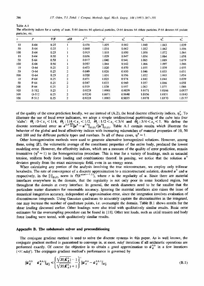
Table A.1

The effectivity indices for a variety of tests. S-64 denotes 64 spherical particles, O-64 denotes 64 ablate particles, P-64 denotes 64 prolate

particles, etc.

7 P FK?F s&B lx” e

10 S-64 0.25 1 0.470

50 S-64 0.25 1 0.848

100 S-64 0.25 1 0.919

10 S-64 0.50 1 0.656

50 S-64 0.50 1 0.917

100 S-64 0.50 1 0.957

10 O-64 0.25 2 0.473

50 O-64 0.25 2 0.849

100 O-64 0.25 2 0.920

10 P-64 0.25 2 0.471

50 P-64 0.25 2 0.847

100 P-64 0.25 2 0.919

100 S-512 0.25 1 0.9228

100 O-512 0.25 2 0.9230

100 P-512 0.25 2 0.9228

77,+ h h h i,

?I! 712 773 r/4

1.025 0.982 1.040 1.043 1.039

1.031 0.962 1.052 1.062 1.056

1.035 0.950 1.058 1.072 1.064

1.029 0.947 1.054 1.064 1.058

1.040 0.941 1.065 1.089 1.079

1.044 0.942 1.066 1.097 1.086

1.020 0.970 1.035 1.039 1.035

1.026 0.950 1.046 1.055 1.051

1.031 0.956 1.052 1.065 1.054

1.025 0.978 1.042 1.044 1.039

1.033 0.960 1.057 1.066 1.058

1.038 0.957 1.063 1.075 1.066

1.0081 0.9839 1.0171 1.0166 1.0157

1.0071 0.9840 1.0156 1.0151 1.0143

1.0083 0.9835 1.0178 1.0170 1.0157

of the quality of the error prediction locally, we use instead of (A.2), the local discrete effectivity indices, 7:. To illustrate the use of local error indicators, we adopt a simple unidirectional partitioning of the cube into four ‘slabs’: @,:O<x,<1/4, @,:1/4<x,<1/2, 0,:1/2<n,<3/4 and 0,:3/4<x,<l. We define the discrete normalized error as eoVh dgf]luh - ~‘,~ll,(~)/II~~ll,(~). Table A.1 contain results which illustrate the behavior of the global and local effectivity indices with increasing mismatches of material properties of 10, 50

and 100 and for different particle types and numbers. In all of these cases, vh = 1. Other homogenization methods were used to generate alternative homogenized solutions. However, among

these, using (E), the volumetric average of the constituent properties of the entire body, produced the lowest

modeling error. However, the effectivity indices, which are a measure of the quality of error prediction, remain insensitive (vh = 1) to the homogenization procedure. This is true for a variety of loadings, such as uniaxial tension, uniform body force loading and combinations thereof. In passing, we notice that the solution u”

deviates greatly from the exact microscopic field, even in an energy norm. When calculating any portion of the analysis involving the true microstructure, we employ only trilinear

hexahedra. The rate of convergence of a discrete approximation to a microstructural solution, denoted uh and u

respectively, in the II.IIECn) norm is B(h min(r-l”)),-where r is the regularity of u. Since there are material

interfaces everywhere in. the domain, that the regularity is not only poor in some localized region, but throughout the domain at every interface. In general, the mesh diameters need to be far smaller that the particulate matter diameters for reasonable accuracy. Ignoring the material interfaces also raises the issue of numerical integration accuracy, independent of approximation error, since the integration involves evaluation of discontinuous integrands. Using Gaussian quadrature to accurately capture the discontinuities in the integrand, one may increase the number of quadrature points, i.e. oversample the domain. Table B.l shows results for the

shear loading discussed earlier. Other loadings were also tried with qualitatively similar results. Basic error estimates for the oversampling procedure can be found in [ 111. Other test loads, such as axial tension and body

force loading were tested, with qualitatively similar results.

Appendix B. The subdomain solver and preconditioning

The conjugate gradient method is used to solve the discrete systems in this paper. As is well known, the conjugate gradient method is guaranteed to converge in, at most, ndof iterations if all arithmetic operations are performed exactly. Of course the objective is to obtain a good approximation to P>h in a few iterations (<< ndof). The conjugate gradient method’s performance is governed by


Table B.l

The effectivity indices for 64 spherical particles and volume fraction of 0.25. E/P denotes elements per particle

7 Gauss-Rule EIP

10 4 27

50 4 21 100 4 27

10 5 27

50 5 21

100 5 27

10 6 21

50 6 27

100 6 27

10 4 216

50 4 216

100 4 216

10 5 216 50 5 216

100 5 216

10 6 216

50 6 216

100 6 216

e 0.h

qh b h h b

71 ?z 93 1)4

0.470 1.025 0.982 1.040 1.043 1.039 0.848 1.031 0.962 1.052 1.062 1.056 0.919 1.035 0.950 1.058 1.072 1.064 0.471 1.024 0.981 1.039 1.042 1.038 0.849 1.030 0.961 1.051 1.061 1.055 0.920 1.034 0.949 1.057 1.071 1.063 0.472 1.023 0.980 1.038 1.041 1.037 0.850 1.029 0.960 1.050 1.060 1.054 0.921 1.033 0.948 1.056 1.070 1.062 0.475 1.016 0.973 1.0;2 1.032 1.029 0.85 1 1.019 0.961 1.039 1.042 1.038 0.92 1 1.021 0.958 1.042 1.047 1.043 0.476 1.015 0.974 1.031 1.031 1.028 0.852 1.018 0.960 1.038 1.041 1.037 0.922 1.020 0.957 1.041 1.046 1.042 0.476 1.015 0.972 1.031 1.031 1.028 0.852 1.018 0.960 1.038 1.041 1.037 0.922 1.020 0.958 1.041 1.046 1.042

where Il.llto denotes the discrete version of the energy norm, X(Ki) is the condition number of the stiffness matrix for s;bdomain K, and i is the iteration number (see [2] for details). As is standard, in an attempt to reduce

the condition number, we invoke preconditioning by forming the foli%wing spsformation of variables, 1:” = PK 4!&, which, produces a local stiffness matrix for subdomain K of K = P,K KPK. Ideally, we would like

PK = LKT where L,.Li = g",, and where L, is a lower triangular matrix, thus forcing

(B.2)

However, the decomposition of the stiffness matrix into a lower triangular matrix and its transpose is comparable in the number of operations to solving the system by Gaussian elimination. Therefore, only an

approximation to L ,k ' A simple and inexpensive preconditioner involves defining PK as a diagonal

matrix with entries lpii = I/ ndc$ where the Kt are the diagonal entries of g”,. In this case the resulting terms in the preconditioned stiffness matrix are unity on the diagonal. The off diagonal terms, #I. are 7-

03.3)


Table. B.2

Selective Subdomain Solves: Local tensile loading over 1/16tl1 of the top surface, YP = 0.3 and NLSS = number of local subdomains

solved and ASIlS = average number of solver iterations per subdomain

7 B/S S NLSS DOFlS ASIIS

10 64 64 14 7500 32

50 64 64 16 7500 43

100 64 64 16 7500 45

10 128 32 6 13125 49

50 128 32 8 13125 64

100 128 32 8 13125 68

10 256 16 3 27375 86

50 256 16 3 27375 107

100 256 16 5 27375 113

It is logical to incorporate the homogenized solution in the preconditioning of the local fine-scale system.

Readily accessible portions of the homogenized solution are the local boundary values, which are the specified boundary conditions on the subdomain interfaces. A penalty method is used to implement local boundary conditions for each subdomain. Afterwards, the previous preconditioning is applied, thus scaling the stiffness

matrix by the boundary values. As an example, consider again the thin ring described in main body of this paper. The number of iterations

needed,for Ifi’ - i’-‘l s O.OOOOO1 are shown in Table B.2. Tests were also run for torsional and radial loading

with qualitatively similar results. It is clear that the solver is relatively robust and insensitive to the mismatch ratio.

Appendix C. Influence of numerical discretization of the subdomain problem

In general, after numerical calculation, the only quantity available is Co**, and it is natural to ask, what does (2{.57(rIoSh) - (.7(u”) - (J’/2)})“” bound?

C.1. A total error relationship

Let us assume that u’. is not calculated exactly, i.e. there is some discretization error. Let us adopt the

following nomenclature: l The finite-dimensional approximation of (21) is characterized by the following statement:

Find ri $” E {ti $“} + Vh(@) such that

5%$&i ;h, u;) = &(ur;c) v u; E Vh(@) .

Therefore, in the case of particulate composites, a reasonable first guess is

EO.0 “2

K 0.0 + 4 po.o Ko.o _; p Kw _ 4 $.O 0 0 0

0.0 2 4 2 K

_- 3 g.0 Ko.o + 3 pwJ Ko.o _ r, $J.o () 0 ()

2 2 4 K

0.0 _- 3 $20 Ko.o _ ~ /p KoJJ + 5 $vJ () () ()

0 0 0 P 0.0

0 0 0 0 0 0 povo 0

0 0 0 0 0 /Lo*

(C.1)

(C-2)


Also, a similar type of approximation can be made for anisotropic media, but using the more general Reuss and Voigt bounds

oo (E-‘)+(E) E‘=- 2 . (C.3)

Srep a. Exploratory moves around E””

I < 3, in sequence by ? 6E “’

are made by perturbing the components of E’.‘, {E::}, 1 G i, j, k,

, +6{Ez$}, 1 < i, j, k, 1 C 3, units. If the perturbation decreases the augmented

potential, the perturbed material parameters are retained, otherwise the original values are kept. After each

component has been tested, the resulting vector is denoted E lzo. If E”” = E ‘,O, go to Step b, otherwise go

to Step c. Since there i.s no directional dependence of the particulate composite material’s macroscopic response, it

is reasonable (as well as inexpensive) to use isotropic perturbations. Furthermore, with isotropic perturbations it is trivial to check for positive definiteness of the homogenized material. For isotropic materials we h.ave

E’sLE = H1’,L f (tr r)Z + Z_L’,~ dev(e) (C.4)

and

Q : E’.Le = K’.L(tr E)~ + 2p’,L(dev(e)) : (dev(c)) . cc.3

where dev(e) = 4 - 3 (tr l )Z. Since the dilatational and deviatoric parts of stress are independently variable,

we must have ‘c’*~ > 0 and (u”~ > 0 to retain positive definiteness of E’,L. We directly perturb K”~ and Z.L”~

and then reconstruct the elasticity tensor:

&‘.L + 4 SP’.L SK’.’ _ 3 s&L &‘.L -$L’.L 0 0 0

6PL - 5 Z&J &.L + 4 Q$L &‘.L +QL 0 0 0

&+L “5 &I,L _ 3 ap’.L Q.L _ ; @.L 6K’,L + 4 8p’3L 0 0 0 * ((33)

0 0 0 8p”L 0 0

0 0 0 0 ?QL 0

0 0 0 0 0 &LL 1

Step b. E”” is the location of the minimum to within a tolerance of Z&Y’.‘. Either each 6{E:i}, 1 G i, j, k,

1 s 3 is reduced, as in the example, and Step a is repeated, or the search is terminated with E’,‘, being the final answer.

Step c. Make a new search to a temporary vector E “’ = 2E ‘.’ -E’.‘. Essentially, E ‘.’ is reached by moving from E”*’ to E Iso and continuing for an equal distance in the same direction. Step d. Make exploratory moves around E ‘.’ similar to the ones around E”.’ described in Step a, for as many times until failure (L times). Call the resulting vector E ‘.L. If E ‘,L = E “’ then go to Step e; otherwise go to Step f. Step e. Set Eoo = EITL and return to Step a. Step jI Set E”” = E I”, E ‘,’ = E IsL and return to Step c.

There are several options to determine which components to perturb. One can simply try and perturb all of them, however this is prohibitively expensive. Of course, combinations of perturbation components, less than the full 21 parameters are not unique, and elementary statistics tells us that there are 21 !l(r!(21 - r)!) such choices of r parameters. For example, if we choose only 2 of the constants to perturb, we have 210 possible combinations groups. The types of perturbations presented here are a subset of more general perturbations presented in [ll]. Of course, this material family is not unique, but it gives some physical feeling to the perturbations, and narrows the choices considerably in the presented case from 210 choices to 1.


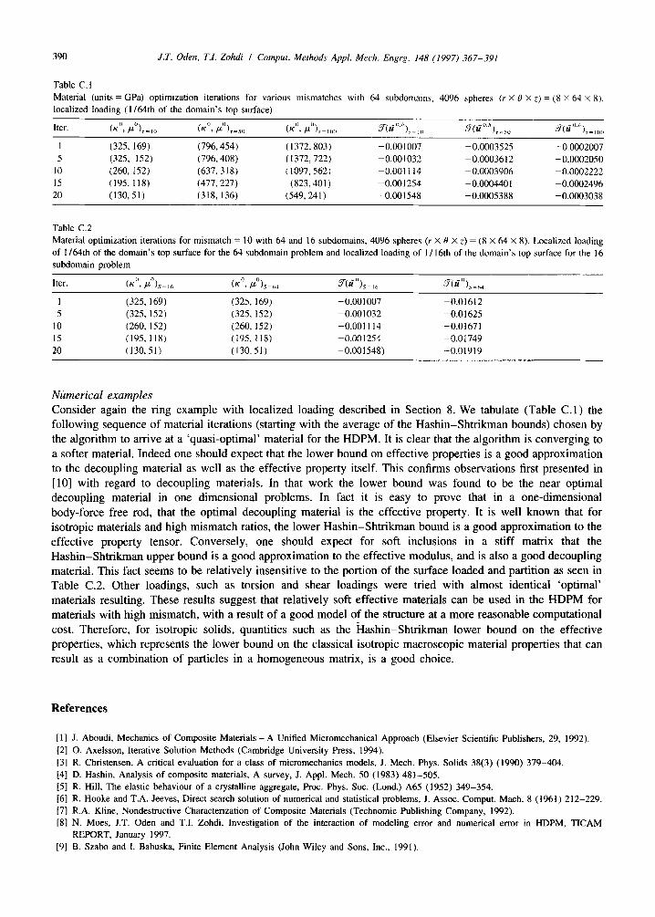
Table C.l

Material (units = GPa) optimization iterations for various mismatches with 64 subdomains, 4096 spheres (r X 0 X :) = (8 X 64 X 8).

localized loading (1/64th of the domain’s top surface)

her. (KC’, $‘),= ,,, (K’l. $‘),=c,I (K”. /*“),= I,,(, Y(ri”~‘),=,,) F((a”.“)_ .W”‘) ,=,,,,,

1 (325,169) (796,454) (1372,803) -0.001007 -0.0003525 - 0.0002007

5 (325, 152) (796,408) (1372,722) -0.001032 -0.0003612 - O.OC02050

10 (260, 152) (637.318) ( 1097,562) -0.ooi 114 -0.0003906 -0.0002222

15 (195. 118) (477,227) (823,401) -0.001254 -0.0004401 -0.0002496

20 (130.51) (318,136) (549,241) -0.001548 -0.0005388 -0.0003038

Table C.2

Material optimization iterations for mismatch = 10 with 64 and 16 subdomains, 4096 spheres (r X 0 X z) = (8 X 64 X 8). Localized loading

of 1/64th of the domain’s top surface for the 64 subdomain problem and localized loading of 1 /I 6th of the domain’s top surface for the I6

subdomain problem

Iter. (K(‘, ~‘l).$= ,h (KO, pYr& W1),=,, W’),=,,

1 (325, 169) (325, 169) -0.001007 -0.01612

5 (325, 152) (325,152) -0.001032 -0.01625

10 (260, 152) (260, 152) -0.001114 -0.01671

15 (195,118) (195. 118) -0.001254 -0.01749

20 (130.51) (130.51) -0.001548) -0.01919

Nbmerical examples

Consider again the ring example with localized loading described in Section 8. We tabulate (Table C.1) the following sequence of material iterations (starting with the average of the Hashin-Shtrikman bounds) chosen by the algorithm to arrive at a ‘quasi-optimal’ material for the HDPM. It is clear that the algorithm is converging to a softer material, Indeed one should expect that the lower bound on effective properties is a good approximation

to the decoupling material as well as the effective property itself. This confirms observations first presented in [lo] with regard to decoupling materials. In that work the lower bound was found to be the near optimal decoupling material in one dimensional problems. In fact it is easy to prove that in a one-dimensional

body-force free rod, that the optimal decoupling material is the effective property. It is well known that for isotropic materials and high mismatch ratios, the lower Hashin-Shtrikman bound is a good approximation to the effective property tensor. Conversely, one should expect for soft inclusions in a stiff matrix that the Hashin-Shtrikman upper bound is a good approximation to the effective modulus, and is also a good decoupling material. This fact seems to be relatively insensitive to the portion of the surface loaded and partition as seen in Table C.2. Other loadings, such as torsion and shear loadings were tried with almost identical ‘optimal’

materials resulting. These results suggest that relatively soft effective materials can be used in the HDPM for materials with high mismatch, with a result of a good model of the structure at a more reasonable computational

cost. Therefore, for isotropic solids, quantities such as the Hashin-Shtrikman lower bound on the effective properties, which represents the lower bound on the classical isotropic macroscopic material properties that can result as a combination of particles in a homogeneous matrix, is a good choice.

References

[II J. Aboudi, Mechanics of Composite Materials - A Unified Micromechanical Approach (Elsevier Scientific Publishers, 29, 1992).

121 0. Axelsson, Iterative Solution Methods (Cambridge University Press, 1994).

[3] R. Christensen, A critical evaluation for a class of micromechanics models, .I. Mech. Phys. Solids 38(3) (1990) 379-404.

[4] D. Hashin, Analysis of composite materials, A survey, J. Appl. Mech. 50 (1983) 481-505.

[5] R. Hill, The elastic behaviour of a crystalline aggregate, Proc. Phys. Sot. (Lond.) A65 (1952) 349-354.

[6] R. Hooke and T.A. Jeeves, Direct search solution of numerical and statistical problems, J. Assoc. Comput. Mach. 8 (1961) 212-229.

[7] R.A. Kline, Nondestructive Characterization of Composite Materials (Technomic Publishing Company, 1992).

[8] N. Moes, J.T. Oden and T.I. Zohdi, Investigation of the interaction of modeling error and numerical error in HDPM, TICAM

REPORT, January 1997.

191 B. Szabo and I. Babuska, Finite Element Analysis (John Wiley and Sons, Inc., 1991).


[IO] T.I. Zohdi, J.T. Oden and G.J. Rodin, Hierarchical modeling of heterogeneous bodies, TICAM REPORT, May 1996 (also to appear in

Computer Methods in Applied Mechanics and Engineering, Jan. 1997).

[1 I] T.I. Zohdi, Error estimation and adaptive methods for the analysis of elastic structures composed of highly heterogeneous media, Ph.D.

Dissertation, The University of Texas at Austin, 1997.

Documents

Analysis #and adaptive modeling of highly heterogeneous