Analysing the relationship between

implied cost of capital metrics and realised stock returns

by

Colin Clubb

King’s College London

and

Michalis Makrominas

Frederick University Cyprus

Draft: September 2017

Comments most welcome, please do not quote.

Abstract

We extend the analytical framework linking realised stock returns and ICC estimates used in Easton

and Monahan (2005) and Mohanram and Gode (2013) (based on Vuolteenaho (2002)) by incorporating

insights from studies by Pettengill, Sundaram, and Mathur (1995) and Hughes, Liu, and Liu (2009). We

use the theoretical work of Hughes et al (2009) to structure our analysis of the relationship between

realised returns and the ICC in order to: (i) take account of the impact of ‘market news’ on the

association between the ICC and realised stock returns; (ii) provide an alternative measure of ‘discount

rate news’; and (iii) take account of the expected theoretical difference between the implied cost of

capital and the expected rate of return. Our empirical results, based on both cross-sectional and time-

series analysis and employing an adjustment for analyst earnings forecast error, are generally consistent

with the implications of our analytical framework. Specifically, our cross-sectional regression results

(a) provide robust support for a coefficient close to one for most ICC estimates after taking account of

market news, (b) provide cash flow news and discount rate news coefficient estimates close to one, and

(c) provide evidence for the role of a growth/leverage based variable as a control for the expected

difference between the ICC and expected stock returns. Time-series results for individual firms confirm

strong mean reversion in ICC estimates as assumed in our analytical framework and provide strong

corroborative evidence for a positive association between market new adjusted implied risk premiums

and realised returns. Overall, our paper provides further robust support for the relevance of realised

returns as a benchmark for establishing the usefulness of ICC measures, consistent with theoretical

expectations.

1

1. Introduction

Previous research has provided evidence on the relationship between a variety of implied cost of capital

(ICC) estimates and realised stock returns. This research is important as reliable cost of capital estimates

are required for optimal investment decision-making by both managers and investors, and the

explanatory power of implied cost of capital estimates for future realised stock returns provides a

potentially important basis for evaluating the usefulness of ICC metrics in this role. As highlighted in

many prior studies, however, the comparison of ICC estimates with realised stock returns is affected by

the impact of new information on stock returns and by potential bias in analysts’ earnings forecasts used

to generate ICC estimates. As a result, more recent theoretical and empirical analysis of this relationship

has focused on controlling for the effect of ‘cash flow news’ and ‘discount rate news’ on realised stock

returns and adjusting analysts’ earnings forecasts for predictable bias. While such controls have led to

improved empirical results providing clear evidence of a positive relationship between ICC estimates

and realised returns, notably by Mohanram and Gode (2013), multivariate regression results

incorporating cash flow news and discount rate news variables are not entirely consistent with

theoretical expectations.

In the current paper, we extend the analytical framework linking realised stock returns and ICC

estimates used in Easton and Monahan (2005) and Mohanram and Gode (2013) (based on

Vuolteenaho’s (2002) analysis of the relationship between realised and expected returns) by

incorporating insights from prior studies by Pettengill, Sundaram, and Mathur (1995) and Hughes, Liu,

and Liu (2009). We use the theoretical work of Hughes et al (2009) to structure our analysis of the

relationship between realised returns and the ICC in order to: (i) take account of the impact of market

movements or ‘market news’ on the association between the implied cost of capital and realised stock

returns, as implied by Pettengill et al (1995); (ii) provide an alternative measure of ‘discount rate news’

based on mean-reverting expected returns; and (iii) take account of the expected theoretical difference

between the implied cost of capital and the expected rate of return highlighted by Hughes et al (2009).

Our empirical results, which also employ an adjustment for analyst earnings forecast error based on

Larocque (2013), are generally consistent with the implications of our analytical framework. More

specifically, our cross-sectional regression results: (a) provide robust support for a coefficient close to

2

one for most ICC estimates (including those based on Ohlson and Juettner-Nauroth (2005) and

Gebhardt, Lee, and Swaminathan (1999)) after taking account of market news; (b) provide cash flow

news and discount rate news coefficient estimates close to one; (c) provide evidence for the role of a

growth/leverage based variable as a control for the expected difference between the ICC and expected

stock returns. Additional time-series results for sample firms provide strong evidence of mean reversion

in ICC estimates and further strong evidence of a positive association between market news adjusted

ICC estimates and realised returns as predicted by theory. In summary, our paper contributes to the

literature by extending analysis of the relationship of the relationship between realised returns and ICC

metrics and providing strong empirical support for a positive association broadly consistent with

theoretical expectations.

The remainder of the paper is organised as follows. Section 2 provides a review of previous

work on ICC and realised returns and highlights the issues which motivate the current study. Section 3

develops our analytical framework linking the ICC to realised stock returns. Section 4 outlines the data,

ICC estimation methods, and empirical models and methods used in the study. Section 5 reports and

discusses our empirical findings based on cross-sectional and time-series analysis of the association

between ICC measures and realised stock returns. Section 6 summarises and concludes the paper.

2. Previous research and motivation

Assumptions regarding expected equity return underpin significant financial decisions

regarding investment, valuation and capital budgeting. While a large volume of literature in finance and

accounting has been devoted to measuring the cost of equity, the problem of validating measures of

expected equity return continues to be an important research issue. We review here some of the key

papers which have used accounting based valuation models to infer the ICC with a particular focus on

evidence on the association of ICC estimates with realised stock returns.

The development of valuation models linking stock prices with future earnings or dividends

based on various assumptions regarding expected performance and asymptotic growth rates has led to

a number of alternative approaches to estimating the ICC. Such approaches include Botosan (1997)

who uses the dividend discount model with a target price as terminal value, Gebhardt et al (2001) who

3

employ the residual income model using short term analyst earnings forecasts and an industry specific

asymptotic growth rate, Claus and Thomas (2001) who implement the residual income model with an

economy wide growth rate, and Gode and Mohanram (2004) who implement the Ohlson and Juettner-

Nauroth (2005) abnormal earnings growth model where short-term earnings growth assumptions are

based on analyst earnings forecasts and long-term growth is based on an economy-wide long term

growth rate. Easton (2004) identifies the price-earnings / growth (PEG) valuation model as a special

case of the Ohlson and Juettner-Nauroth (2005) model and develops a procedure for simultaneously

estimating the ICC and the long-run growth rate given short-run analyst earnings forecasts. Further

studies by Botosan and Plumlee (2005), Easton and Monahan (2005), Botosan et al (2011), Hou et al

(2012), and Mohanram and Gode (2013) provide evidence on the usefulness of a range of ICC estimates

using the association of ICC estimates with ‘known’ risk factors and with realised stock returns as the

main basis for comparison.

Botosan and Plumlee (2005) assess the association of ICC estimates with a range of variables

intended to proxy for risk factors and provide evidence that only two of their ICC measures, based on

the dividend and PEG models, are significantly related to market, leverage, information, and residual

risk proxies. However, given that interest in the ICC method has been reanimated in recent years due

to perceived limitations of the ability of asset factor models to provide reliable estimates of the cost of

capital, this approach appears to have some limitations. These are discussed by Easton and Monahan

(2016) who highlight the apparent conceptual inconsistency of using the asset factor model approach to

evaluate ICC metrics and question the ability of measures such as book-to-price to proxy for ‘true’ risk

factors.1 An alternative approach which does not suffer the conceptual issues related to the risk factor

approach is to evaluate the efficacy of alternative ICC measures to predict future realized returns. This

approach, however, has generated mixed results as indicated below.

In univariate tests of association, Gode and Mohanram (2004) find that ICC estimates derived

from the Ohlson and Juettner-Nauroth (2005) model are only weakly correlated with future realized

1 Berk (1995) questions the interpretation of book-to-price and size as risk factors, a perspective which is

developed by Clubb and Naffi (2007) where they are interpreted as valuation factors rather than risk factors in a

returns model based on Vuolteenaho (2000).

4

returns. Easton and Monahan (2005), using a methodology based on the Vuolteenaho (2002) return

decomposition model, evaluate seven ICC estimates and conclude that none of these estimates show a

meaningful association with realized returns, even after controlling for shocks related to cash flow news

and discount rate news. An important feature of the Easton and Monahan study is the use of changes in

the estimated ICC between consecutive years as the basis for estimating discount rate news. Botosan et

al (2011), on the other hand, provide more supportive results on the association of a wide range of ICC

estimates with realised returns when additional information on the change in analysts target prices

(interpreted as cash flow news) and changes in firm-specific betas and interest rates (interpreted as

expected return news) are included as additional explanatory variable for returns. While their results

are generally consistent with the expected positive association between realised returns and ICC, the

incremental explanatory power of ICC beyond their extensive set of cash flow and expected returns

news control variables is however generally small. Laroque (2013) also provides some further evidence

of a positive association between ICC estimates and realised returns after controlling for cash flow and

expected return news using procedures outlined in Callen and Segal (2010). Finally, Mohanram and

Gode (2013) show that adjusting analysts’ forecasts for predictable errors resulted in a positive

association between returns and a range of ICC estimates using a similar methodology to Easton and

Monahan (2005).2

With the exception of Mohanram and Gode (2013) and Laroque (2013), research on ICC

estimation has typically used analyst earnings forecasts under the assumption that these forecasts match

the market’s earnings expectations. Other research, however, documents important shortcomings in

analyst forecasts such as upward bias (O’Brien (1998)), sluggishness (Mendenhall (1991)) and/or

underreaction (overreaction) to bad (good) news (Easterwood and Nutt (1999)). Furthermore, studies

by Elgers and Lo (1994) and Ali et al (1992) show that analyst forecasting errors can be predicted using

2 Christodolou et al (2014) provide evidence that realised stock returns revert to an estimate of the long-run cost

of equity based on accounting information. Firm cost of equity estimates, however, are extracted from estimation

of time-series accounting information dynamics based on Ohlson (1995) and Clubb (2013) and hence their

approach differs from the ICC methodology of ‘reverse-engineering’ the stock price using accounting information.

The Christodolou et al (2014) analysis therefore provides support for a significant association between realised

stock returns and an accounting-based cost of capital estimate in the long-run but does not address the issue of the

cross-sectional relationship between ICC estimates and short-run stock returns considered in the literature

reviewed here.

5

information available at the time (or prior) to the forecast. More recently, Hughes et al (2008) model

expected forecasting error based on factors related to overreaction (accruals, sales growth, long-term

growth, growth in PP&E) as well as factors related to underreaction (past return, past error, forecast

revision). The potential impact of analyst errors on ICC estimates, highlighted in Claus and Thomas

(2001) and Easton and Monahan (2005), raises the question of whether the validity of ICC estimates

can improve by correcting for analysts expected error. Only a small number of studies consider the

return predictability of ICC estimates after adjusting the imputed forecasts for analyst error. Guay et al.

(2011) adjust forecasts for errors related to analyst underreaction (past return), size effects, analyst

following and book to market. They find that once predictable errors have been removed the return

predictability of ICC estimates improve, but the improvement is limited at portfolio level and for some

ICC estimates. Larocque (2013) extends Ali et al (1992) to construct an error-correction model

encompassing past forecast error, recent return, size and a control for measurement error but fails to

find an improvement in ICC return predictability once analyst forecast have been adjusted. More

positively, as previously indicated, Mohanram and Gode (2013) use the Hughes et al (2008) model to

remove predictable errors for analysts forecasts and document a substantial improvement in the

association of ICC estimates and future realized returns when controlling for cash flow news and

discount news.

While the study by Mohanram and Gode (2013) provides the strongest evidence to date that a

wide range of ICC metrics based on the residual income and abnormal earnings growth models can

provided significant explanatory power for future realised stock returns with a consistently positive

ICC coefficient, their results are not entirely consistent with theory. Specifically, the coefficient for

most ICC metrics turns out to be significantly different from the theoretical expectation of 1 and the

coefficient for discount rate news is either significantly negative (rather than positive as expected by

theory) or insignificantly different from 0. Based on the insight of Pettengill et (1995) that the

relationship between realised returns and expected returns will be affected by returns on the market

portfolio in a simple CAPM setting (and, for example, will be negative when realised returns on the

market are below the risk-free rate), we propose a ‘market news’ adjustment to ICC estimates to control

for the impact of unexpected market returns on the association between realised returns and ICC

6

metrics. While such market news is incorporated within the theoretical measures of ‘cash flow news’

and ‘discount rate news’ provided by the Vuolteenaho (2002) return decomposition, it is unclear that

the empirical proxies used for these news variables in Easton and Monahan (2005) and Mohanram and

Gode (2013) fully capture market news. The following section of the paper develops an analytical

framework which incorporates all three news measures and provides the basis for our empirical analysis

in sections 4 and 5 of the paper. Given the importance of controlling for analyst forecast bias suggested

by the findings of Mohanram and Gode (2013), our subsequent empirical analysis also uses an error

correction model to control for predictable analyst forecast errors based on Laroque (2013). While the

use of this methodology did not significantly improve her findings, she provided other evidence on the

utility of the adjustment procedure which suggests its potential usefulness on our larger sample of US

stocks.

In summary, previous research has provided weak or mixed evidence on the association

between ICC metrics and realised stock returns. We develop an analytical framework which builds on

the Vuolteenaho (2002) based framework of Easton and Monahan (2005) and Mohanram and Gode

(2013) by incorporating theoretical insights from Hughes et al (2009) and taking account of the possible

impact of market return news on the association between ICC metrics and realised returns in the spirit

of Pettengill et al’s (1995). Based on our framework, the empirical analysis extends previous research

in three important respects; first, the impact of market news on the return/ICC relationship is exposed;

second, broad support is provided for ICC and news variables coefficients with sign and magnitude

predicted by theory: third, evidence of bias in ICC estimates as estimates of expected stock returns is

indicated. We interpret our analysis and empirical findings as contributing significantly to the growing

evidence on the usefulness of ICC based approaches to estimating the cost of capital.

3. Modelling the relationship between realised stock returns and the implied cost of capital

Our analysis of the relationship between realised stock returns and the implied cost of capital

integrates insights from previous studies by Pettengill et al. (1995), Vuolteenaho (2002), Easton and

Monahan (2005), and Hughes et al. (2009). First, we assume an underlying single factor asset pricing

model as in Hughes et al (2009) and show how the relationship between realised stock returns and

7

expected stock returns is affected by realised market returns, as highlighted previously by Pettingill et

al (1995). Second, we combine this model of realised returns with the return decomposition model of

Vuolteenaho (2002) where realised stock returns are expressed as the summation of expected returns,

cash flow news, and discount rate news and confirm that realised stock returns can be expressed as the

sum of expected returns adjusted for (or conditional on) market returns and firm-specific cash flow and

discount rate news. Third, given results in Hughes et al (2009) on differences between ICC and expected

returns, we consider the impact of using the implied cost of capital (rather than expected returns) in our

model of realised returns and show how this leads to a division of realised stock returns into three main

elements:

(i) market news adjusted implied cost of capital,

(ii) firms specific news based on changes in the implied cost of capital and cash flow news,

(iii) error related to the difference between the implied cost of capital and expected returns.

Fourth, we consider the implications of this division of realised stock returns for empirical analysis of

the relationship between stock returns and implied cost of capital. Finally, we propose a linear

regression model for assessing this relationship empirically.

3.1 Realised returns and market news adjusted expected returns

Following Hughes et al (2009), our analysis assumes that expected returns are generated by the

following single factor market model (firm subscripts are suppressed for presentational clarity):

𝜇𝑡𝑡+1 = 𝑟𝑓 + 𝜆𝛽𝑡

𝑡+1 (1)

where 𝜇𝑡𝑡+1 is expected return for period t+1 as at end of period t, 𝛽𝑡

𝑡+1 is beta for period t+1 estimated

(and known with certainty) at the end of period t, 𝜆 is the market risk premium (assumed constant over

time), and 𝑟𝑓 is the risk-free rate (again assumed constant over time). Also consistent with Hughes et

al. (2009), we assume that:

𝛽𝑡𝑡+1 = 𝛽 + 𝜎𝛽𝜀𝛽𝑡 (2)

where 𝜀𝛽𝑡 , 𝑡 = 0,1, … … . ∞, are standard normal variates, and that 𝛽𝑡𝑡+𝑠 = 𝛽 for s > 1 so that:

𝜇𝑡𝑡+𝑠 = 𝑟𝑓 + 𝜆𝛽 ≡ 𝜇, for 𝑠 > 1 (3)

8

Drawing on the observation of Pettengill et al (1995) that the relationship between realised returns and

beta is conditional on realised market returns, realised returns for t+1 can be written as:

𝑟𝑡+1 = 𝜇𝑡𝑡+1 + (𝜆𝑡+1 − 𝜆)𝛽𝑡

𝑡+1 + 𝜖𝑡+1 (4)

where 𝜆𝑡+1 represents the realised market return for period t+1 less the risk-free rate and 𝜖𝑡+1 is a mean

zero disturbance term reflecting idiosyncratic firm risk during period t+1. Subtracting 𝑟𝑓 from both

sides of equation (4) and substituting for 𝛽𝑡𝑡+1 using equation (1) then gives:

𝑟𝑡+1∗ =

𝜆𝑡+1

𝜆𝜇𝑡

𝑡+1∗+ 𝜖𝑡+1 (5)

where 𝑟𝑡+1∗ ≡ 𝑟𝑡 − 𝑟𝑓 and 𝜇𝑡

𝑡+1∗≡ 𝜇𝑡

𝑡+1 − 𝑟𝑓.

3.2 Realised returns, market news adjusted expected returns, and firm-specific cash flow and

discount rate news

Vuolteenaho (2002) and Easton and Monahan (2005) show that if earnings are measured on a

clean surplus basis and the log of the book-to-market ratio has an unconditional mean (i.e, is mean-

reverting), realised stock returns for period t+1 may be written (approximately) as:

𝑟𝑡+1 = 𝜇𝑡𝑡+1 + ∑ 𝜌𝑗(𝑥𝑡+1

𝑡+1+𝑗− 𝑥𝑡

𝑡+1+𝑗)

∞

𝑗=0

− ∑ 𝜌𝑘(𝜇𝑡+1𝑡+1+𝑘 − 𝜇𝑡

𝑡+1+𝑘)

∞

𝑘=1

(6)

where 𝑥𝑡𝑡+1+𝑗

denotes the expectation of the log of one plus accounting return on equity for period

t+1+j as at the end of period t and 𝜌 can be viewed as a discount factor for aggregating changes in

expectations of future accounting return on equity and future expected stock returns.3 Equation (6)

indicates that realised returns are equal to expected returns plus ‘total firm news’ for the period, where

‘total firm news’ is divided into ‘cash flow news’, ∑ 𝜌𝑗(𝑥𝑡+1𝑡+1+𝑗

− 𝑥𝑡𝑡+1+𝑗

)∞𝑗=0 , and ‘discount rate news’,

− ∑ 𝜌𝑘(𝜇𝑡+1𝑡+1+𝑘 − 𝜇𝑡

𝑡+1+𝑘)∞𝑘=1 . Using equation (3) to simplify the discount rate news component of

equation (6) and re-expressing in terms of excess returns over the risk-free rate gives:

𝑟𝑡+1∗ = 𝜇𝑡

𝑡+1∗+ ∑ 𝜌𝑗(𝑥𝑡+1

𝑡+1+𝑗− 𝑥𝑡

𝑡+1+𝑗)

∞

𝑗=0

− 𝜌(𝜇𝑡+1𝑡+2∗

− 𝜇∗) (7)

3 As discussed in Easton and Monahan (2005), 𝜌 lies between 0 and 1 and is likely to be positively related to the

price-to-net dividend ratio. Empirical estimation of 𝜌 based on firms divided into price-to-dividend quartiles

suggests that it lies between 0.92 and 1.

9

where 𝜇∗ ≡ 𝜇 − 𝑟𝑓 and, which from comparison with equation (5), implies that:

𝜖𝑡+1 = ∑ 𝜌𝑗(𝑥𝑡+1𝑡+1+𝑗

− 𝑥𝑡𝑡+1+𝑗

)

∞

𝑗=0

− 𝜌(𝜇𝑡+1𝑡+2∗

− 𝜇∗) − (𝜆𝑡+1

𝜆− 1) 𝜇𝑡

𝑡+1∗ (8)

Equation (8) indicates that ‘firm-specific news’, represented by 𝜖𝑡+1 in equation (5), is equal to cash

flow news plus discount rate news minus market news given by (𝜆𝑡+1

𝜆− 1) 𝜇𝑡

𝑡+1∗, where market news

contains both market-related cash flow news and market-related discount rate news.

3.3 Realised returns, market news adjusted implied cost of capital, firm-specific cash flow and

discount rate news, and error in the implied cost of capital

In order to provide an expression for evaluating the relationship between realised stock returns

for period t+1 and the ICC at the end of period t, denoted by 𝜋𝑡, we define ‘excess ICC’ (over the risk-

free rate) as 𝜋𝑡∗ ≡ 𝜋𝑡 − 𝑟𝑓, add and subtract (

𝜆𝑡+1

𝜆𝜋𝑡

∗ − 𝜌(𝜋𝑡+1∗ − 𝜋𝑡

∗)) from the right hand side of

equation (5), and make use of equation (8) to obtain:

𝑟𝑡+1∗ =

𝜆𝑡+1

𝜆𝜋𝑡

∗ + [∑ 𝜌𝑗(𝑥𝑡+1𝑡+1+𝑗

− 𝑥𝑡𝑡+1+𝑗

) − 𝜌(𝜋𝑡+1∗ − 𝜋𝑡

∗)

∞

𝑗=0

− (𝜆𝑡+1

𝜆− 1) 𝜋𝑡

∗]

+ {(𝜇𝑡𝑡+1∗

− 𝜋𝑡∗) − 𝜌 ((𝜇𝑡+1

𝑡+2∗− 𝜇∗) − (𝜋𝑡+1

∗ − 𝜋𝑡∗))} (9)

Equation (9) indicates that excess realised returns can be expressed as the sum of the following three

components:

Market news adjusted excess ICC equal to 𝜆𝑡+1

𝜆𝜋𝑡

∗ = 𝜋𝑡∗ + (

𝜆𝑡+1

𝜆− 1) 𝜋𝑡

∗, where (𝜆𝑡+1

𝜆− 1) 𝜋𝑡

∗

represents a measure of ‘market news’ based on excess ICC (rather than excess expected returns

as in equation (5))

Firm-specific news (given by the term in square brackets) equal to cash flow news plus discount

rate news minus market news, where discount rate news and market news are based on excess

ICC (rather than excess expected returns as in equation (8)), and

ICC error (given by the final term in curly brackets) resulting from use of excess ICC instead

of excess expected return (i) as the main explanatory variable i.e., (𝜇𝑡𝑡+1∗

− 𝜋𝑡∗) and (ii) as the

basis for measuring discount rate news i.e., −𝜌 ((𝜇𝑡+1𝑡+2∗

− 𝜇∗) − (𝜋𝑡+1∗ − 𝜋𝑡

∗)).

10

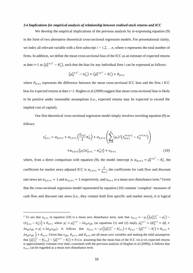
3.4 Implications for empirical analysis of relationship between realised stock returns and ICC

We develop the empirical implications of the previous analysis by re-expressing equation (9)

in the form of two alternative theoretical cross-sectional regression models. For presentational clarity,

we index all relevant variable with a firm subscript i = 1,2, …n, where n represents the total number of

firms. In addition, we define the mean cross-sectional bias of the ICC as an estimate of expected returns

at date t+1 as (�̅�𝑡𝑡+1∗

− �̅�𝑡∗), such that the bias for any individual firm i can be expressed as follows:

(𝜇𝑖𝑡𝑡+1∗

− 𝜋𝑖𝑡∗ ) = (�̅�𝑡

𝑡+1∗− �̅�𝑡

∗) + 𝜗𝑖𝑡+1

where 𝜗𝑖𝑡+1 represents the difference between the mean cross-sectional ICC bias and the firm i ICC

bias for expected returns at date t+1. Hughes et al (2009) suggest that mean cross-sectional bias is likely

to be positive under reasonable assumptions (i.e., expected returns may be expected to exceed the

implied cost of capital).

Our first theoretical cross-sectional regression model simply involves rewriting equation (9) as

follows:

𝑟𝑖𝑡+1∗ = 𝛼0,𝑡+1 + 𝛼1,𝑡+1 (

𝜆𝑡+1

𝜆𝜋𝑖𝑡

∗ ) + 𝛼2,𝑡+1 (∑(𝜌𝑖)𝑗(𝑥𝑖𝑡+1𝑡+1+𝑗

− 𝑥𝑖𝑡𝑡+1+𝑗

)

∞

𝑗=0

)

+𝛼3,𝑡+1(𝜌𝑖(𝜋𝑖𝑡+1∗ − 𝜋𝑖𝑡

∗ )) + 𝜐𝑖𝑡+1 (10)

where, from a direct comparison with equation (9), the model intercept is 𝛼0,𝑡+1 = �̅�𝑡𝑡+1∗

− �̅�𝑡∗, the

coefficient for market news adjusted ICC is 𝛼1,𝑡+1 =𝜆

𝜆𝑡+1, the coefficients for cash flow and discount

rate news are 𝛼2,𝑡+1 = 1 and 𝛼3,𝑡+1 = 1 respectively, and 𝜐𝑖𝑡+1 is a mean zero disturbance term.4 Given

that the cross-sectional regression model represented by equation (10) contains ‘complete’ measures of

cash flow and discount rate news (i.e., they contain both firm specific and market news), it is logical

4 To see that 𝜐𝑖𝑡+1 in equation (10) is a mean zero disturbance term, note that 𝜐𝑖𝑡+1 = −𝜌𝑖 ((𝜇𝑖𝑡+1

𝑡+2 ∗− 𝜇𝑖

∗) −

(𝜋𝑖𝑡+1∗ − 𝜋𝑖𝑡

∗ )) + 𝜗𝑖𝑡+1 where 𝜇𝑖∗ = 𝜇𝑖𝑡

𝑡+1∗− 𝜆𝜎𝑖𝛽𝜀𝑖𝛽𝑡 (as equations (1) and (2) imply 𝜇𝑖𝑡

𝑡+1∗= 𝜆𝛽𝑖𝑡

𝑡+1 = 𝜆𝛽𝑖 +

𝜆𝜎𝑖𝛽𝜀𝑖𝛽𝑡 = 𝜇𝑖∗ + 𝜆𝜎𝑖𝛽𝜀𝑖𝛽𝑡). It follows that 𝜐𝑖𝑡+1 = −𝜌 ((�̅�𝑡+1

𝑡+2∗− �̅�𝑡+1

∗ ) + 𝜗𝑖𝑡+2 − (�̅�𝑡𝑡+1∗

− �̅�𝑡∗) + 𝜗𝑖𝑡+1 +

𝜆𝜎𝑖𝛽𝜀𝑖𝛽𝑡 ) + 𝜗𝑖𝑡+1. Given that 𝜀𝑖𝛽𝑡, 𝜗𝑖𝑡+1, and 𝜗𝑖𝑡+2 are all mean zero variables and making the mild assumption

that (�̅�𝑡+1𝑡+2∗

− �̅�𝑡+1∗ ) − (�̅�𝑡

𝑡+1∗− �̅�𝑡

∗) ≈ 0 (i.e. assuming that the mean bias of the ICC vis-à-vis expected returns

is approximately constant over time, consistent with the previous analysis of Hughes et al (2009)), it follows that

𝜐𝑡+1 can be regarded as a mean zero disturbance term.

11

that the coefficient for these variables should equal 1 and that the coefficient for market news adjusted

ICC should in effect ‘undo’ the market news adjustment i.e., 𝛼1,𝑡+1 (𝜆𝑡+1

𝜆𝜋𝑖𝑡

∗ ) =𝜆

𝜆𝑡+1(

𝜆𝑡+1

𝜆𝜋𝑖𝑡

∗ ) = 𝜋𝑖𝑡∗ .

On the other hand, if we assume that market news for firm i can be split into a market cash flow news

component, 𝑚𝑖𝑡+1𝐶𝐹 , and a market discount rate news component, 𝑚𝑖𝑡+1

𝐷𝑅 , where 𝑚𝑖𝑡+1𝐶𝐹 + 𝑚𝑖𝑡+1

𝐷𝑅 =

(𝜆𝑡+1

𝜆− 1) 𝜋𝑖𝑡

∗ , and that this market news is not captured by cash flow and discount rate news variables,

then the following alternative theoretical cross-sectional regression model is implied by equation (9):

𝑟𝑖𝑡+1∗ = 𝛼0,𝑡+1 + 𝛼1,𝑡+1 (

𝜆𝑡+1

𝜆𝜋𝑖𝑡

∗ ) + 𝛼2,𝑡+1 (∑(𝜌𝑖)𝑗(𝑥𝑖𝑡+1𝑡+1+𝑗

− 𝑥𝑖𝑡𝑡+1+𝑗

)

∞

𝑗=0

− 𝑚𝑖𝑡+1𝐶𝐹 )

+𝛼3,𝑡+1(𝜌𝑖(𝜋𝑖𝑡+1∗ − 𝜋𝑖𝑡

∗ ) − 𝑚𝑖𝑡+1𝐷𝑅 ) + 𝜐𝑖𝑡+1 (11)

where the coefficient on market news adjusted ICC is now 𝛼1,𝑡+1 = 1 (and 𝛼0,𝑡+1 = �̅�𝑡𝑡+1∗

− �̅�𝑡∗,

𝛼2,𝑡+1 = 1 and 𝛼3,𝑡+1 = 1). A possible rationale for the omission of market news from cash flow news

based on analyst forecasts is provided in Appendix A.

The cross-sectional regression models represented by equations (10) and (11) indicate that while

use of market news adjusted ICC in place of unadjusted ICC does not alter the explanatory power of

one particular cross-sectional regression (because 𝜆𝑡+1

𝜆 is a scale factor applied to each firm’s ICC

estimate in the date t+1 regression), it will affect the time-series distribution of the regression coefficient

over the whole sample period and hence inferences based on the time-series mean (such as those based

on Fama-MacBeth t statistics). In particular, if market news is not well captured by empirical estimates

of cash flow and discount rate news, equation (11) implies that market news adjustment of ICC estimates

should generate a time-series mean coefficient more reliably close to 1.5 On the other hand, if market

5 Based on equation (11), if the realised excess market return deviates significantly from 𝜆 over time and market

news represented by (𝜆𝑡+1

𝜆− 1) 𝜋𝑡

∗ is not reflected in estimates of cash flow and discount rate news for firms, the

mean time-series coefficient for ICC without market news adjustment (equal to the time series mean of 𝜆𝑡+1

𝜆 ) will

be volatile and may be significantly different from 1. The coefficient for the market news adjusted ICC in this

setting, on the other hand, is exactly 1 in all years.

12

news is well captured by cash flow and discount rate news proxies, equation (10) suggests that the mean

coefficient based on ICC estimates without market news adjustment should be more reliably close to 1.6

In summary, our analytical framework provides the basis for our empirical approach which

accommodates the possibility that cash flow and discount rate news proxies do not fully capture market

news. More specifically, it provides a basis for testing whether market news adjustment of ICC estimates

leads to an improved specification of the relationship between realised stock returns and the ICC. In

section 4, we outline our empirical research models based on this analysis after discussing our dataset

and the alternative ICC metrics used in the study.

4. Data, variable estimation methods, and empirical models

4.1 Data

We consolidate consensus analyst forecasts from the I/B/E/S summary file, accounting data from

COMPUSTAT and market data from CRSP. Risk free rates are obtained from the publicly available

feed of U.S. Treasury. All data is collected 6 months prior to estimation date so as to allow accounting

data to become publicly available and thus incorporated into analyst forecasts and stock prices. Since

I/B/E/S coverage starts from 1981 and given our data requirement of 1-year ex-post market return our

full sample covers the period between 1982 and 2013.

To facilitate meaningful estimates from the Ohlson and Juettner-Nauroth (2005) (OJ hereafter)

or abnormal earnings growth model, we eliminate firm-year observations with negative earnings per

share estimates. Likewise, we eliminate some observations for which the numerical solutions for the

Gebhardt et al (2001) and Claus and Thomas (2001) (GLS and CT respectively hereafter) specifications

of the residual income valuation model do not converge to valid estimates. We furthermore sacrifice

three years of observations in the interest of adjusting implied cost of capital for predictable analyst

errors. Finally, we remove observations with extreme values of prices (P0 <0.5 or P0 >500).

6 This is the converse of the case considered in footnote 4. Specifically, based on equation (10), if the realised

excess market return deviates significantly from 𝜆 over time and market news represented by (𝜆𝑡+1

𝜆− 1) 𝜋𝑡

∗ is

completely reflected in cash flow and discount rate news, the mean time-series coefficient for market news

adjusted ICC (equal to the time series mean of 𝜆

𝜆𝑡+1 ) will be volatile and may be significantly different from 1.

The coefficient for the ICC without market news adjustment in this case, on the other hand, will be exactly 1 in

all years.

13

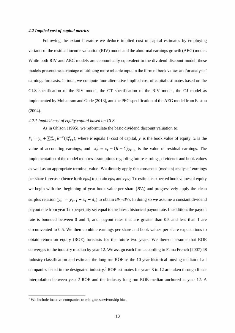
4.2 Implied cost of capital metrics

Following the extant literature we deduce implied cost of capital estimates by employing

variants of the residual income valuation (RIV) model and the abnormal earnings growth (AEG) model.

While both RIV and AEG models are economically equivalent to the dividend discount model, these

models present the advantage of utilizing more reliable input in the form of book values and/or analysts’

earnings forecasts. In total, we compute four alternative implied cost of capital estimates based on the

GLS specification of the RIV model, the CT specification of the RIV model, the OJ model as

implemented by Mohanram and Gode (2013), and the PEG specification of the AEG model from Easton

(2004).

4.2.1 Implied cost of equity capital based on GLS

As in Ohlson (1995), we reformulate the basic dividend discount valuation to:

𝑃𝑡 = 𝑦𝑡 + ∑ 𝑅−𝜏(𝑥𝑡+𝜏𝛼∞

𝜏=1 ), where R equals 1+cost of capital, yt is the book value of equity, xt is the

value of accounting earnings, and 𝑥𝑡𝛼 = 𝑥𝑡 − (𝑅 − 1)𝑦𝑡−1 is the value of residual earnings. The

implementation of the model requires assumptions regarding future earnings, dividends and book values

as well as an appropriate terminal value. We directly apply the consensus (median) analysts’ earnings

per share forecasts (hence forth epst) to obtain eps1 and eps2. To estimate expected book values of equity

we begin with the beginning of year book value per share (BV0) and progressively apply the clean

surplus relation (𝑦𝑡 = 𝑦𝑡−1 + 𝑥𝑡 − 𝑑𝑡) to obtain BV1-BV2. In doing so we assume a constant dividend

payout rate from year 1 to perpetuity set equal to the latest, historical payout rate. In addition: the payout

rate is bounded between 0 and 1, and, payout rates that are greater than 0.5 and less than 1 are

circumvented to 0.5. We then combine earnings per share and book values per share expectations to

obtain return on equity (ROE) forecasts for the future two years. We thereon assume that ROE

converges to the industry median by year 12. We assign each firm according to Fama French (2007) 48

industry classification and estimate the long run ROE as the 10 year historical moving median of all

companies listed in the designated industry.7 ROE estimates for years 3 to 12 are taken through linear

interpolation between year 2 ROE and the industry long run ROE median anchored at year 12. A

7 We include inactive companies to mitigate survivorship bias.

14

terminal value based on the industry ROE of the last year completes the valuation. There are is no closed

form solution to obtain implied cost of capital estimates under the current implementations of the

residual income model (a 12th-degree polynomial). We thus obtain numerical solutions with errors less

than or equal to 10(-10) (maximum 50 Newton iterations).

4.2.2 Implied cost of equity capital based on CT

In this implementation we similarly apply the consensus (median) analysts’ earnings per share

forecasts to obtain eps1 and eps2 and then use the analysts’ long term growth prediction (hence forth

ltg) to estimate eps3-eps5. When the ltg estimate is not available this variable is set equal to the industry

median. A terminal value is obtained by assuming that all future earnings grow at the rate of inflation

set equal to the long term risk free rate (10 year government bond) minus 3% (rf-3%).

4.2.3 Implied cost of equity capital based on the OJ model

The abnormal earnings growth model or OJ model expresses the value of a firm's stock as a

function of the cost of capital, expected earnings, and long term earnings asymptotic growth. The

functional form of the model is given by:

𝑃0 =𝑒𝑝𝑠1

𝑟[1 +

𝑔2

𝑅 − 𝛾]

where 𝑔2 = [%Δ 𝑒𝑝𝑠2 + 𝑟𝑑𝑝𝑠1

𝑒𝑝𝑠1] − 𝑟, R equals 1+the cost of capital, r is the cost of capital and γ is the

long term asymptotic growth rate. Rearranging for r one obtains:

𝑟 = Α + √Α2 +𝑒𝑝𝑠1

𝑃0(𝑔 − (𝛾 − 1))

where 𝐴 =1

2{(𝛾 − 1) +

𝑑𝑝𝑠1

𝑃0}, γ is the long term asymptotic earnings’ growth rate and g is the short

term earnings’ growth rate. Following the assumptions made in Mohanram and Gode (2013) we equate

the short term rate with the geometric mean of the two year growth in earnings per share (eps2/eps1 -1)

and the long term growth rate (ltg). Where the short term growth is lower than ltg, the short term growth

rate is set equal to ltg. Furthermore, as in the RIV models dps1 is set equal to the latest historical dividend

payout while the asymptotic growth rate (γ-1) equals rf-3%.

15

4.2.4 Implied cost of equity capital based on PEG ratio

Setting the asymptotic growth rate equal to zero, such as (γ-1 = 0), and assuming a zero dividend

payout rate the OJ model simplifies to: 𝑟 = √(𝑒𝑝𝑠2 − 𝑒𝑝𝑠1)/𝑃0 ,or equivalently to 𝑟 = √(𝑒𝑝𝑠1

𝑃) ∗ 𝑔,

where g is the short term earnings’ growth rate. The assumption that (γ-1 = 0) corresponds to a special

case of the OJ model where the expected abnormal earnings growth between year 1 and year 2 is an

unbiased estimate of expected abnormal earning growth in all subsequent periods (Easton (2004)).

Following the assumptions made in the full OJ model we set g equal to the average of the two year

growth in earnings per share (eps2/eps1 -1) and the long term growth rate (ltg) when the two year growth

in earnings is greater than ltg, or equal to ltg when the two year growth rate is less than ltg.

4.3 Adjusting implied cost of capital for predictable analyst errors

Implied cost of capital estimates are calculated using analysts’ forecasts under the assumption

that these forecasts are in line with the market’s earnings expectations. Nevertheless analysts’ forecasts

are subject to well documented biases including optimism (O’ Brien (1998)) and sluggishness (Guay et

al (2011)). Deviations between analysts’ forecasts and market expectations embedded in implied cost

of capital estimates are likely to impair the return predictability of these estimates. On the other hand,

accounting for expected bias should mitigate the mismatch between earnings forecasts and market

prices thus improving the implied cost of capital estimates.

A number of research papers including Guay et al (2011) and Hughes et al (2008) construct

multivariate models to predict analyst errors using contemporary and/or historical variables. In a more

recent development, Larocque (2013) models analyst expected error as a function of lagged error,

abnormal stock return, market value and a control for measurement error, and finds that that error-

adjusted forecasts are improved estimates of market’s earnings expectations. To that end we opt to

replicate the Larocque (2013) model. The description of the model and estimated coefficients can be

found in Appendix B.

To construct an out-of-sample test, we run 3-year rolling regressions of the multivariate

forecasting model and apply the coefficients of each regression to the subsequent year's realizations of

the corresponding explanatory variables to get predicted values of analysts expected forecasting errors.

16

Finally, we correct the analyst earnings forecasts by subtracting the estimated values of expected

forecasting errors from the original values of these forecasts. Using the “corrected earnings” we repeat

the estimation procedure of alternative implied cost of capital specifications thus obtaining a set of

“adjusted” ICC estimates.

4.4 Empirical regression models

4.4.1 Cross-sectional analysis of relationship between realised returns and ICC metrics

Our main empirical analysis is based on cross-sectional estimation of regression models

developed from our analytical framework. In addition, however, we also provide some time-series tests

of mean reversion in our ICC estimates

Based on equations (10) and (11), the main empirical regression model for examining the

explanatory power of alternative ICC metrics for stock returns is as follows:

𝑅𝐸𝑇𝑖,𝑡+1 = 𝛼0 + 𝛼1𝑀𝐼𝑅𝑃𝑖,𝑡 + 𝛼2𝐶𝑁𝐸𝑊𝑆𝑖,𝑡+1 + 𝛼3𝐷𝑁𝐸𝑊𝑆𝑖,𝑡+1 + 𝛼4𝐺𝑅𝐿𝑉𝐺𝑖,𝑡. +𝜀𝑖,𝑡+1 (12)

where:

𝑅𝐸𝑇𝑖,𝑡+1 is the excess realised return for firm i over the risk-free rate during year t+1;

𝑀𝐼𝑅𝑃𝑖,𝑡 = 𝐼𝑅𝑃𝑖,𝑡 × 𝑀𝑁𝐸𝑊𝑆𝑡+1 where:

𝐼𝑅𝑃 𝑖,𝑡 ≡ 𝐼𝐶𝐶𝑖,𝑡 − 𝑟𝑓𝑡 is the implied risk premium for firm i at the end of year t based on the

difference between estimated implied cost of capital, 𝐼𝐶𝐶𝑖,𝑡, and the 10 year US Treasury bond

rate, 𝑟𝑓𝑡, at that date;

𝑀𝑁𝐸𝑊𝑆𝑡+1 is the market news adjustment estimated as the ratio of the excess realised market

returns over the risk-free rate to the market equity risk premium (assumed to be 6% in most of

our analysis);

𝐶𝑁𝐸𝑊𝑆𝑖,𝑡+1 is cash flow news at date t+1 using the method employed by Easton and Monahan (2005);8

8 CNEWS is measured using a similar approach to Easton and Monahan (2005) and Mohanram and Gode (2013)

as follows:

𝐶𝑁𝐸𝑊𝑆𝑖,𝑡+1 = {𝑟𝑜𝑒𝑖𝑡+1 − 𝑓𝑟𝑜𝑒𝑖𝑡+1,𝑡+1)} + {𝑓𝑟𝑜𝑒𝑖𝑡+1,𝑡+1 − 𝑓𝑟𝑜𝑒𝑖𝑡,𝑡+1} +𝜌

(1 − 𝜌𝜔𝑡)

∗ {𝑓𝑟𝑜𝑒𝑖𝑡+1,𝑡+2 − 𝑓𝑟𝑜𝑒𝑖𝑡,𝑡+2}

where froeij,k is the forecasted return on equity of firm i, for the fiscal year k, based on the consensus earnings

forecast released in year j. As such the first term of CNEWS represents the realized forecast error on the eps

forecast made at the end of fiscal year t+1 (scaled by beginning book value per share), the second term represents

the forecast revision between the time of the estimation of implied cost of capital until the end of the fiscal year,

and the third term represents the revision in the two-year forecasted return on equity adjusted by a capitalization

factor equal to ρ/(1- ρ *ωt). Estimates of ρ are taken from Easton and Monahan (2005) and vary between 0.924

and 0.988 across five quintiles based on dividend to price ratios. The term ωt captures time series persistence in

ROE and is estimated through a pooled rolling regression for each of the 48 Fama and French (1997) industries

using 10 years of lagged data, such as: 𝑟𝑜𝑒𝑖,𝑡−𝜏 = 𝜔0 + 𝜔𝑡 ∗ 𝑟𝑜𝑒𝑖,𝑡−𝜏−1, where τ takes the values between 0 and

17

𝐷𝑁𝐸𝑊𝑆𝑖,𝑡+1 ≡ −𝜌(𝐼𝑅𝑃 𝑖,𝑡+1 − 𝐼𝑅𝑃 𝑖,𝑡) is the estimated discount rate news measured for firm i for year

t+1, where 𝜌 is an estimate of the Vuolteenaho (2002) capitalisation factor as estimated by Easton and

Monahan (2005);

𝐺𝑅𝐿𝑉𝐺𝑖,𝑡 = 𝐺𝑅𝑖,𝑡 × 𝐿𝑉𝐺𝑖,𝑡 where:

𝐿𝑉𝐺𝑖,𝑡 ≡ 1 + 𝐷𝑖,𝑡 𝐸𝑖,𝑡⁄ where 𝐷𝑖,𝑡 is the estimated market value of debt and 𝐸𝑖,𝑡 is the estimated

market value of equity for firm i as at the end of year t;

𝐺𝑅𝑖,𝑡 is equal to one plus the growth rate for firm i as estimated at the end of year t where the

growth rate varies according to the ICC metric under consideration. For GLS it is based on the

10-year industry ROE median, for CT it is based on the inflation adjusted long-term risk free

rate, and for OJ and PEG models it is based on the average of short term growth rate (eps2/ eps1-

1) and long term rate (ltg) earnings growth rate when (eps2/ eps1-1) is greater than ltg, or equal

to ltg when (eps2/ eps1-1) is less than ltg.

While the rationale for including 𝑀𝐼𝑅𝑃𝑖,𝑡, 𝐶𝑁𝐸𝑊𝑆𝑖,𝑡+1, and 𝐷𝑁𝐸𝑊𝑆𝑖,𝑡+1 follows directly from our

analysis in section 3, the inclusion of 𝐺𝑅𝐿𝑉𝐺𝑖,𝑡 requires some explanation. Also the calculation of

𝐷𝑁𝐸𝑊𝑆𝑖,𝑡+1 differs from that in previous research and requires some further explanation.

The rationale for including 𝐺𝑅𝐿𝑉𝐺𝑖,𝑡 is based on the Hughes et al (2009) analysis of factors

which cause the ICC to be a biased indicator of next period expected stock returns. As indicated in our

analysis summarised in equations (10) and (11) in section 3, the intercept term captures average bias,

while the disturbance term 𝜐𝑖𝑡+1 includes the effect of firm-specific bias represented by 𝜗𝑖𝑡+1, and 𝜗𝑖𝑡+2

(see earlier discussion in footnote 3). The analysis of Hughes et al (2009) and Lambert (2009) suggest

that the downward bias in ICC will be positively related to volatility of cash flows and expected returns

and that this bias will be amplified for firms with higher growth and higher leverage. We therefore

include 𝐺𝑅𝐿𝑉𝐺𝑖,𝑡 in equation (12) to provide an additional control for the bias of (even accurate) ICC

estimates as indicators of expected returns.

The definition of 𝐷𝑁𝐸𝑊𝑆𝑖,𝑡+1 ≡ −𝜌(𝐼𝑅𝑃 𝑖,𝑡+1 − 𝐼𝑅𝑃 𝑖,𝑡), where 𝜌 is an estimate of the

Vuolteenaho (2002) capitalisation factor as estimated by Easton and Monahan (2005), differs from the

definition used by Easton and Monahan (2005) and Gode and Mohanram (2013) due to our assumption

that expected returns follow a mean-reverting process as in Hughes et al (2009) (see our equation (3)

9. CNEWS is a firm-specific, model independent variable which varies across firm-year observations but remains

constant across alternative ICC models.

18

and its use to obtain equation (7)). The alternative assumption made by Easton and Monahan (2005)

and Gode and Mohanram (2013) is that expected returns follow a random walk with −𝜌/(𝜌 − 1) (rather

than simply – 𝜌) used to determine 𝐷𝑁𝐸𝑊𝑆𝑖,𝑡+1. As reported in section (5), our assumption of mean

reversion appears to result in a more reasonable coefficient for 𝐷𝑁𝐸𝑊𝑆 closer to the theoretical

benchmark of 1.

In our empirical analysis reported in section (5), we estimate equation (12) cross-sectionally

for each year over our 32 year sample period and calculate Fama-MacBeth (1973) t-tests on the annual

mean coefficents with Newey-West (1987) autocorrelation adjusted standard errors. For comparative

purposes, we also estimate a regression of the form of equation (12) but with 𝐼𝑅𝑃 𝑖,𝑡 in place of 𝑀𝐼𝑅𝑃 𝑖,𝑡.

In addition, we estimate some additional regressions where 𝐶𝑁𝐸𝑊𝑆𝑖,𝑡+1, 𝐷𝑁𝐸𝑊𝑆𝑖,𝑡+1, and 𝐺𝑅𝐿𝑉𝐺𝑖,𝑡

are excluded in order to determine the importance of these variables as explanatory variables for stock

returns. If our analysis represented by equation (11) is correct and 𝐶𝑁𝐸𝑊𝑆𝑖,𝑡+1 and 𝐷𝑁𝐸𝑊𝑆𝑖,𝑡+1 do

not adequately capture 𝑀𝑁𝐸𝑊𝑆𝑡+1, we expect 𝛼1, 𝛼2, and 𝛼3 to equal approximately 1. Given Hughes

et al (2009) suggest that the average excess of expected returns and implied cost of capital may be of

the order of 2.3% for plausible volatility assumptions, we also expect 𝛼0 > 0. Finally, given that our

𝐺𝑅𝐿𝑉𝐺𝑖,𝑡 variable has an overall mean over all ICC metrics of about 2.0, and assuming an average

impact of this ICC bias variable of say 1% to 2% (or 0.01 to 0.02), one might expect a positive

coefficient for 𝛼4 of the order of 0.005 to 0.010. While the precise magnitude of 𝛼4 cannot be readily

predicted, we clearly expect it to be positive and statistically significant but of much smaller magnitude

in comparison to 𝛼1, 𝛼2, and 𝛼3.

4.4.2 Time series analysis of ICC mean reversion and association with realised returns

In addition to our cross-sectional analysis, we run firm-by-firm time series tests on mean

reversion in our implied cost of capital estimates to provide further evidence on our previous assumption

that ICC reverts immediately to its long-run mean. We also run further time-series tests of the

association between realised returns and estimated ICC to check for consistency with our main cross-

sectional results. The time-series models we run are summarised below, a more detailed rationale for

the proposed models is provided in Appendix C.

19

To test for mean reversion, we estimate the following simple AR1 model for each firm / ICC

time-series where the number of consecutive ICC estimates is at least 20 years:

𝐼𝐶𝐶𝑡+1 = 𝑎0 + 𝑎1𝐼𝐶𝐶𝑡 + 𝑒𝑡+1 (13)

where, assuming 𝑎0 > 0 and 0 ≤ 𝑎1 < 1, the long-run mean ICC estimate is given by 𝑎0 (1 − 𝑎1)⁄ . As

discussed in Appendix C, our analysis suggests that it is likely that the residuals in equation (13) will

serially correlated. For this reason, we estimate equation (13) using maximum likelihood rather than

OLS. For approximate consistency with our calculation of DNEWS in equation (12), we expect 𝑎1 to

be close to 0, thereby indicating rapid mean reversion of the ICC (and the underlying expected returns).

As discussed further in Appendix C, our analytical framework in section 3 also suggests the

following time-series estimation of the relationship between excess realised stock returns and the

market news adjusted implied return risk premium for each firm / ICC time series:

𝑅𝐸𝑇𝑡+1 = 𝑏0 + 𝑏1𝑀𝐼𝑅𝑃𝑡+𝑒𝑡+1 (14)

where 𝑏1 is expected to equal 1 and 𝑏0 is expected to equal 0 for the special case where the ICC measures

next period expected returns without error i.e, where 𝜋𝑡∗ = 𝜇𝑡

𝑡+1∗ in terms of our analytical framework.

Given our argument in section 3.4 based on Hughes et al (2009) that in general 𝜋𝑡∗ < 𝜇𝑡

𝑡+1∗, we show

in Appendix C that it is likely that 𝑏1 in equation (14) will be biased above 1 and that 𝑏0 will be positive,

reflecting the average downward bias of the ICC as an estimator of the expected stock return.

5. Empirical results

5.1 Descriptive statistics for model variables

Table 1 Panel A provides descriptive statistics for key variables used to estimate ICC metrics.

Mean price and book value per share figures for our sample imply an average price to book ratio above

2.0, while the average industry median ROE (based on the 48 industries in Fama and French (1997))

for our sample period is 14%. Mean short term forecast eps growth is 59% but this is inflated by some

large positive figures, suggesting that the median figure of 19% is a more representative summary

statistic. The mean long-term earnings forecast growth of 15% is close to the median of 14% indicating

no undue influence of extreme values on this figure. Indeed, as expected, the standard deviation 10%

20

implies a moderate spread of long-term eps growth forecasts, in marked contrast to the distribution of

short-term growth rates.

Table 1 Panel B provides summary statistics for estimated implied risk premia for the four

alternative ICC metrics used in the study. The OJ model provides the highest mean and median implied

risk premia estimates consistent with higher long-run earnings growth for this model. The residual

income based models, GLS and CT, have the lowest median implied risk premia reflecting lower long

term growth compared with the abnormal earning growth based metrics (OJ and PEG). Overall, implied

risk premia are somewhat low compared with previous research findings based on the equity risk

premium (the median IRP varies between 3.15% for CT and 5.47% for OJ), possibly reflecting the

tendency of the ICC approach to underestimate expected returns highlighted by Hughes et al (2009).

Table 2 provides the correlation matrix between implied risk premia based on our four ICC

metrics. In general, these are statistically significant at the 1% for all years for all metrics with the

exception of one year in the case of CT metric. There are, however, clear differences between the metric,

the Pearson correlation coefficient exceeding 0.60 only for association between the OJ and PEG metrics.

The correlation for the latter of 0.94 is unsurprising given that the PEG model is a special case of the

more OJ abnormal earnings growth model. It would seem that the common short-term growth rate used

in PEG and OJ estimates of the ICC drive this high pairwise correlation and that the substantially higher

median and mean implied risk premium for the OJ model is due to long-term growth assumed in the

latter.

Finally, Table 3 provides descriptive statistics for all variables used in the estimation of

equation (12). The table indicates that controlling for predictable analyst forecast error using the

Larocque (2013) methodology results in substantially lower estimated risk premiums, consistent

broadly with analyst optimism. In relation to the news variables included in our main empirical analysis,

CNEWS is on average only 0.34% but has a substantial standard deviation of 8.65%, while DNEWS for

all four metrics is on average close to zero with a standard deviation ranging between 1.47% for GLS

and 7.55% for CT. The variation in CNEWS and to a lesser degree DNEWS is therefore consistent with

volatile stock returns which deviate substantially from expected returns. The MNEWS variable has a

mean of 0.94 and median of 1.53 indicating a tendency for market returns to exceed our expected market

21

risk premium of 6% in most years but for large negative market returns to pull the mean market return

close to the assumed expected market risk premium. The substantial number of negative values for

MNEWS (the 25th percentile is negative) highlights the problem of an expected negative association

between implied risk premium estimates and realised excess stock returns in several years and hence

the potential usefulness of using MIRP in place of IRP in empirical tests of the association between

stock returns and ICC metrics.

5.2 Cross-sectional findings for implied risk premiums excluding market news adjustment

Table 4 provides regression results for the explanatory power of implied risk premiums for

excess realised stock returns without an adjustment for market news. Panel A reports results based on

estimation of the ICC metrics using analysts’ earnings forecasts unadjusted for error and Panel B reports

results based on ICC metrics estimated using error-corrected analyst earnings forecasts. The univariate

results based on IRP reported in Panel A have very low R2 and counterintuitively negative slope

coefficients. Addition of CNEWS and DNEWS variables greatly improves explanatory power and all

coefficients for these news variables are significantly positive at the 1% level for all four ICC metrics.

The improved explanatory power of the GLS based model is particularly strong, the adjusted R2

increasing from 1.80% for the univariate model to 10.42% for the models with the additional news

variable. However, for all ICC metrics, the coefficient for IRP is remains negative.

Panel B of Table 4 shows a major improvement in the performance of the IRP variable when it

is based on ICC estimated using Larocque (2013) error-corrected analyst earnings forecasts. Similar to

results reported by Mohanram and Gode (2013) based on the Hughes et al (2008) error adjustment

procedure, the analyst error adjustment leads to highly significant positive coefficients for IRP in GLS,

OJ, and PEG univariate regressions which are in excess of 1 (the IRP coefficient however remains

significantly negative for the CT regression). Inclusion of CNEWS and DNEWS variables adds further

to the explanatory power of the regression models, adjusted R2 increasing to 10% or above for GLS,

OJ, and PEG based metrics. There are also substantial reductions in estimated coefficients for IRP,

although these remain significantly above the theoretical value of 1 (1.40 for GLS and 1.55 and 1.91

respectively for OJ and PEG metrics). Interestingly, the coefficient for DNEWS based on our

assumption of mean reversion in expected returns is consistently positive in regressions for all metrics

22

and is relatively close to the benchmark of 1, most notably for GLS. In summary, the results in Table 4

confirm previous findings of improvements in the explanatory power of ICC for realised stock returns

when ICC estimates are adjusted for analyst forecast error and when cash flow and discount rate news

variables are included in the regression model.

Table 5 provides further evidence on the positive association of ICC estimates with realised

stock returns using a portfolio based methodology employed by Hou et al (2012). More specifically,

Table 5 provides strong support for the hypothesis that a portfolio of the top IRP decile of stocks have

significantly higher one-year ahead realised returns than a portfolio of the bottom IRP decile of stocks

for all four ICC metrics. These results, based on analyst error-corrected ICC estimates, are in contrast

to the results reported by Hou et al (2012) for an average of unadjusted analyst earnings forecast based

ICC estimates where there was no statistically significant difference between top and bottom decile

portfolio returns. The results reported in Table 5 therefore reinforce the regression results in Table 4

Panel B highlighting the important contribution of analyst error correction to establishing the validity

of ICC estimates.

5.3 Cross-sectional findings for market news adjusted implied risk premiums

Table 6 provides regression results for the explanatory power of implied risk premiums for

realised stock returns when the implied risk premium is adjusted for market news i.e., when the variable

MIRP is used in place of IRP. In addition, the growth / leverage variable GRLVG, intended to capture

the impact of variation in the bias of ICC as an estimator for expected returns as highlighted in Hughes

et al (2009), is also included in the full model results (based on equation (12)). As previously, Panel A

reports results based on estimation of the ICC metrics using analysts’ earnings forecasts unadjusted for

error and Panel B reports results based on ICC metrics estimated using the Larocque (2013) error-

corrected analyst earnings forecasts. In addition

Results reported in Panel A of Table 6 indicate that the coefficient for MIRP is positive in a

simple univariate regression model and is statistically significant at the 10% level for GLS and PEG

metrics. The addition of CNEWS and DNEWS variables results in additional explanatory power together

with statistically significant positive coefficients for MIRP for all metrics at the 5% level or better.

23

However, the results in Panel A based on unadjusted analyst earnings forecasts fall well short of the

benchmark coefficient of 1 for MIRP and the GRLVG is statistically insignificant in all regressions.

Panel B of Table 6 indicates that analyst error correction in the estimation of ICC metrics

combines with the market news adjustment of the implied risk premium to generate results where

coefficients for MIRP, CNEWS and DNEWS coefficients are generally closest to the benchmark of 1

(only for DNEWS is the null hypothesis that the coefficient equals 1 widely rejected) and the coefficient

for GRLVG is positive as expected and statistically significant at the 5% level or better for CT, OJ and

PEG metrics. Focusing on the results for the full model represented by equation (12), GLS, CT, OJ, and

PEG coefficients for MIRP are 1.14, 0.63, 1.07, and 0.82 respectively, all of which are significantly

positive at the 1% level and, with just the exception of the CT model, insignificantly different from the

benchmark of 1. Furthermore, for all metrics, the coefficient for CNEWS is significant at the 1% level

and generally close to the benchmark of 1. DNEWS coefficients vary across metrics but are significantly

positive in all cases (although below 1 for OJ, PEG, and CT models and above 1 for GLS). Finally, the

GRLVG variable is significant and positive for all metrics except GLS and of a reasonable magnitude

in relation to expectations discussed in section 4. Given that GRLVG should capture cross-sectional

variation in the bias of the IRP as an estimate of true expected returns and the intercept should capture

common bias across all firms for a particular IRP, the significantly positive intercepts for GLS and PEG

regressions and significantly positive GRLVG coefficients for CT, OJ, and PEG regressions in Panel B

of Table 6 are consistent with the Hughes et al (2009) hypothesis that ICC estimates are downwardly

biased estimates of the true expected return.

The results for all four ICC metrics in Panel B of Table 6 are broadly consistent with equation

(11) in our analytical framework. In other words, our results support the assumption that CNEWS and

DNEWS estimated using the methods described in section 4.3 of this paper provide useful firm-specific

news but do not fully capture market news. With market news adjustment of implied risk premia, results

are close to theoretical expectations for these three metrics. Which metric performs best according to

our analysis? It could be argued that the OJ model performs best in terms of a small and statistically

insignificant intercept together with highly significant MIRP and CNEWS coefficients very close to the

theoretical ideal of 1. The GLS regression, on the other hand, has the highest average adjusted R2 and

24

a MIRP coefficient that is also not significantly different from 1, suggesting that the GLS metric has a

similarly meaningful association with stock returns to the OJ metric. The PEG model association with

realised returns is similar in many respects to OJ model but is a little weaker in terms of explanatory

power and proximity of coefficients to theoretical expectations. The CT model has coefficients of

correct sign but there is some statistical evidence that the MIRP coefficient is less than 1 counter to

expectations and its explanatory power is slightly weaker than the other models.

Finally, as discussed in Appendix A(iii), it is useful to consider the effect of excluding any

possible impact of market news on our measure of cash flow news. Results from estimating our full

model given by equation (12) where CNEWS is replaced with an alternative cash flow news variable,

CNEWS*, which has been orthogonalied with respect to market news are reported in Panel C of Table

6. For all metrics, the removal of the market news impact on cash flow news leads to increased average

adjusted R2, most notably increasing from 12.61% (in Panel B) to 20.47% for the case of the OJ model.

Furthermore, for GLS, OJ, and PEG, the positive coefficient for MIRP is highly statistically significant

and remains statistically indistinguishable from its theoretical value of 1 at the 10% level and above.

While the coefficient for CNEWS* is substantially higher than that for CNEWS (in Panel B) and is

greater than 1 at the 1% level, the coefficients for DNEWS and GRLVG strengthen slightly compared

with the previous results based on unadjusted CNEWS. Taking the results reported in Panels B and C

of Table 6 together, we conclude that there is some evidence that market news impacts on CNEWS and

that excluding this impact from cash flow news leads to a stronger association between realised returns

and implied cost of capital metrics. In relation to the relative performance of the ICC metrics, the results

in Panel C of Table 6 confirm the previous results in Panel B that the OJ and GLS metrics are most

closely associated with realised stock returns.

5.4 Mean reversion of ICC estimates and time-series findings for market news adjusted implied risk

premiums

As discussed in section 4.4.2 and Appendix C, we carry out additional firm-by-firm time series

tests of mean reversion in ICC estimates in order to provide evidence on the accuracy of the Hughes et

al (2009) assumption that expected rates of return and related ICC estimates are mean-reverting. In

addition, we also provide results on firm-by-firm time series test of the contemporaneous relationship

25

between excess realised returns and estimates of the market news adjusted implied risk premium which

broadly corroborate our previous cross-sectional findings on the robust relationship between ICC

metrics and realised returns.

Results on mean reversion of our ICC estimates are summarised in Table 7 and Figure 1 and

provide broad support for our approach to measuring DNEWS based on the assumption of mean

reversion. Panel A of Table 7 indicates that the mean intercept from estimating equation (13) for our

sample of 1,133 firms with 10 or more annual observations lies in the range of 0.06 to 0.08 and that

individual firm intercepts for all ICC metrics are generally highly statistically significant as evidenced

by the very large proportion of statistically significant positive intercepts (based on a 1% level binomial

test, the requirement for rejection of the null hypothesis of a zero average intercept is 137 significantly

positive intercepts at the 10% level out of 1,133 which is clearly much less than actual figures ranging

from 888 for the CT model to 982 for the OJ model). Rapid mean reversion of all ICC metrics to a long-

run average is supported by low but statistically significant mean slope coefficents which range between

0.05 for PEG and OJ models to 0.14 for the CT model. The estimated mean long-run ICC for all metrics

is therefore only slightly above the mean intercepts and ranges from 7% for the CT model to 9% for the

OJ model. Furthermore, as shown in Panel B of Table 7 and in Figure 1, the overall cross-firm

distribution of the long-run average ICC for all metrics is very similar and relatively symmetric, with a

range of 6% to 7% between the 5th percentile firm and the 95th percentile firm for all metrics. Finally,

our expectation that the intercept from an AR1 regression based on the ICC is a downwardly biased

estimate of the intercept from an AR1 regression based on the true expected return (as indicated by the

intercepts in equations (C2) and (C4) in Appendix C when 𝜑3 < 0) suggests that the long-run expected

return is likely to be in a range somewhat above the long-run ICC range of 7% to 9% shown in Table

7. For example, if the OJ model provides an accurate measure of the ICC, the long-run average ICC of

9% may imply a long-run expected rate of return of 10% or above.

As an alternative time-series perspective on the relationship between ICC estimates and realised

stock returns, we provide evidence from firm-by-firm time series regressions of realised excess returns

on IRP and MIRP variables in Panels A and B of Table 8. Broadly consistent with the cross-sectional

results shown in Panel B of Table 4, the results in Panel A of Table 8 provide support for a positive

26

association between realised returns and IRP for the GLS, OJ, and PEG metrics. Thus, for these metrics,

the mean slope coefficient is equal to 1.87 for PEG, 2.24 for OJ, and 2.60 for GLS and the number of

positive statistically significant coefficients at the 10% level equal to 239 for PEG, 286 for OJ and 285

for GLS substantially exceed that expected by chance at the 1% level according to a binomial test. The

mean coefficients for these models are, however, substantially greater than the theoretical expectation

of 1 and the number of intercepts significantly different from zero is greater than expected by chance.

There is also evidence that the number of slope coefficients out of all 1,133 firms which significantly

deviate from the expected value of 1 is greater than expected by chance.

Panel B of Table 8 provides evidence on the impact of using market news adjusted implied risk

premiums in our time-series regressions which is broadly consistent with the analytical framework in

section 3 and further analysis in Appendix C. As expected, and consistent with the previous analysis of

Pettingill et al (1995), the use of MIRP in place of IRP as the explanatory variable for realised returns

leads to substantially improved results. Most notably, mean/median slope coefficients are close to 1 for

GLS (0.83/0.84), OJ (0.95/0.84), and PEG (0.84/0.85) and the number of positive coefficients at the

10% level for these metrics (534, 605, and 509 for GLS, OJ, and PEG respectively) greatly exceeds the

binomial test cut-off of 137 at the 1% level. However, despite the close proximity of mean and median

slope coefficients to 1, the number of coefficients for which it is possible to reject the null hypothesis

of 1 at the 10% level is substantially greater than the 1% binomial test cut-off of 137 (i.e., 216, 209, and

206 for GLS, OJ, and PEG respectively), thus providing evidence of a small but statistically significant

deviation of the slope coefficient from 1. Consistent with our expectation of downward average bias in

the ICC as an estimate of expected stock returns, mean intercepts are positive and statistically significant

in terms of the number of observed positive estimates exceeding the 1% binomial test cut-off for all

metrics. Finally, as in our cross-sectional results, OJ, GLS, and PEG metrics are superior to the CT

model in terms of overall association with stock returns, with the OJ and GLS metrics performing

slightly more strongly than the PEG model both in terms of the number of sample firms showing the

expected positive association with realised returns and in terms of mean adjusted R2 across firm-level

regressions.

27

Overall, our time-series results corroborate our previous cross-sectional results that for all ICC

metrics there is a highly significant positive association between realised stock returns and MIRP and

that in the case of OJ, GLS, and PEG the estimated slope coefficient is close to the predicted value of

1. Estimation of firm AR1 time-series models for all metrics also strongly supports our theoretical

assumption of rapid mean reversion in the ICC (and hence expected returns) towards a long-term

average of similar magnitude for all metrics (in the 7-9% range based on the means across our sample

of 1,133 firms). Interestingly, the means of the long-run average firm ICC estimates in Panel A of Table

7 are broadly in line with (but slightly lower than) the means of the annual average IRP estimates

reported in the final row of Panel B of Table 1 based on a long-run average risk-free rate of 4%.

5.5 Summary of relationship to previous research findings

Our findings extend previous findings by Mohanram and Gode (2013) which highlighted the

usefulness of removing predictable analyst forecast errors on the explanatory power of ICC metrics for

realised returns. Specifically, we show how an alternative adjustment procedure based on Laroque

(2013) has a similarly significant impact on this relationship, our results in Table 4 Panel B indicating

that application of this procedure to our dataset generates IRP, CNEWS and DNEWS coefficients

substantially closer to theoretical expectation of 1 than in Mohanram and Gode (2013), with the notable

exception of the CT metric (see their Table 8 Panel B). The use of an alternative DNEWS measure based

on the Hughes et al (2009) assumption of mean-reverting expected returns also contributes to DNEWS

coefficients much closer to the theoretical ideal of 1 in comparison to the previous findings in

Mohanram and Gode (2013), where some such coefficients were even perversely negative.

The market news adjustment of IRP estimates and the addition of an ICC bias variable GRLVG,

also motivated by the analysis of Hughes et al (2009), generates theoretically plausible coefficients for

MIRP and news variables in Table 6 Panels B and C for all ICC metrics. The proximity of MIRP

coefficients to 1 is comparable to the previous findings of Botosan et al (2011) but is achieved using a

more parsimonious model which reflects our focus on evaluating ICC metrics. More specifically, the

use of the change in analysts’ target prices and other information including the change in beta over the

return interval by Botosan et al (2013) raises issues regarding the extent of the role of the ICC in driving

their regression results. Our adoption of the Easton and Monahan (2005) and Gode and Mohanram

28

(2013) approach to estimating CNEWS and DNEWS provides a more focused analysis of the importance

of ICC estimates in explaining realised returns because (i) DNEWS is based directly on the relevant ICC

metric and (ii) CNEWS is simply a common control variable used in all regressions based on an ROE

forecast model which is not directly affected by actual changes in the stock price of firms over the return

interval. Our cross-sectional analysis combining a particular IRP measure with the related DNEWS

variable based on the change in the IRP therefore provides a more complete representation of the role

of the given metric per se in explaining realised returns.9

Finally, we extend previous research on the implied cost of capital by providing additional firm-

based time-series results on the association between realised stock returns and the implied cost of

capital. Our results show that after adjusting ICC estimates for realised market returns in the spirit of

Pettengill et al’s (1995) empirical analysis of the CAPM, there is a robust positive association between

stock returns and ICC metrics with slope coefficients for OJ, GLS, and PEG close to (but on average

slightly less than) the expected value of 1. We interpret these results as providing strong corroboration

of our previous cross-sectional results on the relevance of ICC estimates for explaining realised stock

returns.

6. Conclusion

This paper provides a framework for analysing the relationship between realised stock returns

and the implied cost of capital which integrates insights from previous research by Pettengill et al

(1995), Hughes et al (2009), Vuolteenaho (2002), and Easton and Monahan (2005). This framework

suggests that interacting the firm’s implied risk premium with market news (represented by realised

excess market returns over the risk-free rate scaled by the market risk premium) in a regression model

for stock returns which also includes cash flow news and discount rate news variables may lead to

results more consistent with theoretical expectations. Specifically, if cash flow news and discount rate

9 The average adjusted R-squared reported for our full model reported in Table 6 Panels B and C is in the 10%-

20% range. Results reported in Botosan et al’s (2013) Table 6 (p.1108) are typically in the 25%-30% range.

However, as can be seen from comparing the results for their model 1 which excludes the ICC metric (i.e., only

contains other information) with their model 2 results which includes an ICC metric, the incremental role of the

ICC metrics are generally small in their study. For example, while the average R-squared for their model 1

excluding ICC is 25.9%, this rises only modestly to 27.3% when the OJ metric is added and to 28.0% for the GLS

metric.

29

news exclude (or only imperfectly reflect) market news, our framework suggests that market news

adjusted ICC estimates, along with cash flow news and discount rate news, will be required to jointly

explain stock returns. The likely bias of the implied cost of capital as a measure of expected stock

returns identified in previous research is also incorporated into the framework via inclusion of a further

variable based on the interaction of expected earnings growth and financial leverage.

Empirical results reported in the paper provide substantial support for the relevance of the

proposed analytical framework and also highlight the importance of controlling for predictable analyst

forecast error when estimating the ICC. Cross-sectional results indicate that market news adjusted

implied risk premiums for three of our four ICC metrics based on earnings forecasts adjusted for

predictable analyst errors are positively related to stock returns with coefficients statistically

indistinguishable from unity as predicted by theory (estimated coefficients for CNEWS and DNEWS

variables are also strongly positive, the former generally statistically indistinguishable from 1 as

suggested by theory, the latter generally somewhat less than 1). Positive mean intercepts together with

a positive coefficient for our growth leverage interaction variable provide also support to our hypothesis

that the ICC is a downwardly biased estimate of expected returns. In addition, firm-based time-series

analysis strongly confirms the positive association between market news adjusted implied risk

premiums and realised excess stock returns with mean slope coefficients only slightly less than unity

and further supports our assumption of rapid mean reversion in firm based ICC estimates (and hence

expected returns) over time.

In summary, our paper contributes to the research literature by demonstrating conceptually and

empirically the relevance of implied cost of capital metrics for explaining realised stock returns.

Incorporating market news information into the analysis of the relationship between stock returns and

ICC metrics based on analyst forecasts adjusted for predictable error yields results which are closely

related to theoretical expectations. This in turn highlights the importance of ICC estimates based on

residual income and abnormal earning growth models as inputs into assessments of a firm’s required

rate of return on investment.

30

Table 1: Summary statistics of implied risk premia metrics and relevant inputs

PANEL A: Summary statistics for inputs to implied risk premia metrics

Variable N Mean StdDev 25th Pcl Median 75th Pcl 95th Pcl

Price 45,978 29.23 22.48 14.88 24.25 37.44 67.50

BVPS 45,978 13.17 11.63 6.23 10.39 16.76 32.47

Payout 45,978 0.19 0.20 0.01 0.13 0.39 0.50

IROE 1,440 0.14 0.02 0.13 0.14 0.15 0.18

eps1 45,978 1.33 1.50 0.55 1.01 1.72 3.42

eps2 45,978 1.61 1.80 0.75 1.26 2.02 3.97

ltg (%) 45,978 0.15 0.10 0.10 0.14 0.20 0.30

stg (%) 45,978 0.59 3.22 0.13 0.19 0.31 1.55

γ-1 (%) 32 (Years) 0.02 0.02 0.01 0.02 0.04 0.08

PANEL B: Summary statistics of implied risk premia metrics by year (%)

Year N

GLS CT OJ PEG

Mean Median Mean Median Mean Median Mean Median

1982 364 2.59 2.03 4.35 2.74 8.25 6.33 2.98 1.69

1983 552 1.19 -0.59 4.31 1.52 6.30 4.79 1.83 0.60

1984 632 -0.25 -0.37 2.99 2.15 6.08 4.94 1.55 0.88

1985 719 0.39 0.16 2.67 1.79 5.63 4.42 1.54 0.74

1986 765 1.50 1.58 2.47 1.78 4.98 4.22 1.96 1.41

1987 805 1.56 1.59 2.82 1.97 5.33 4.58 2.56 1.81

1988 843 1.71 1.68 2.42 1.88 4.78 4.05 1.73 1.00

1989 904 1.87 1.76 2.98 1.63 4.82 3.77 1.82 0.82

1990 940 1.80 1.73 3.22 1.48 5.23 4.15 2.24 1.19

1991 983 2.23 2.14 3.68 1.95 6.04 4.74 3.34 1.97

1992 1,059 2.18 2.07 2.94 1.78 5.33 4.51 3.00 2.18

1993 1,272 3.07 2.97 3.39 2.37 5.49 4.83 3.62 2.86

1994 1,519 2.53 2.54 3.23 2.66 5.48 4.81 3.45 2.82

1995 1,757 2.69 2.77 3.30 2.66 5.27 4.65 3.24 2.61

1996 1,940 2.68 2.84 3.13 2.42 5.18 4.41 3.21 2.52

1997 2,077 2.54 2.54 3.53 2.44 5.17 4.57 3.28 2.73

1998 2,261 3.42 3.39 4.28 2.91 5.94 5.24 4.38 3.61

1999 2,087 4.08 3.92 5.17 3.37 6.63 5.54 4.88 3.73

2000 1,863 3.87 3.83 4.36 3.53 6.51 5.70 4.53 3.73

2001 1,636 4.18 4.02 4.78 3.42 6.62 5.66 5.02 3.97

2002 1,540 4.43 4.11 6.10 3.46 6.71 5.76 5.33 4.26

2003 1,659 4.99 4.88 7.80 3.56 7.00 5.94 5.67 4.60

2004 1,843 4.07 3.84 8.84 2.66 6.52 5.10 5.03 3.95

2005 2,050 4.32 4.20 7.45 3.23 6.64 5.62 5.16 4.45

2006 1,981 3.58 3.60 6.68 2.86 6.02 5.16 4.38 3.87

2007 2,007 3.71 3.68 10.58 3.22 7.07 5.66 5.59 4.33

2008 1,873 5.64 5.48 7.19 4.25 7.60 6.66 5.98 5.22

2009 1,509 6.69 6.29 9.37 4.51 8.16 7.04 6.56 5.51

2010 1,441 6.08 5.84 11.37 4.86 8.51 7.17 7.16 5.98

2011 1,724 6.14 5.89 10.80 4.58 8.67 7.40 7.52 6.24

2012 1,713 7.75 7.14 12.73 5.70 10.09 8.39 8.91 7.24

2013 1,660 6.42 6.12 10.27 4.41 8.79 7.48 7.79 6.30

All Years 45,978 3.85 3.70 6.14 3.15 6.58 5.47 4.68 3.74

31

Notes: Panel A presents summary statistics for inputs to implied cost of capital estimation. Price is the stock price

measured at the time of implied cost of capital estimation. BVPS is the beginning of year book value deflated by number

of shares outstanding. Payout is the latest realized payout rate. Furthermore, the payout rate is bounded between 0 and 1,

and, payout rates that are greater than 0.5 and less than 1 are circumvented to 0.5. IROE is the industry median rate of

return across all 48 industries based on the Fama and French (1997) classification. eps1 and eps2 are analyst mean

earnings per share forecasts for future years 1 and 2. ltg is the mean long term growth rate projected by analysts. stg is

the short term earnings’ growth equal to (eps2 - eps1)/eps1. γ -1 is long term asymptotic earnings’ growth rate. Panel B

presents annual mean and median statistics of implied risk premia. GLS is the implied risk premium imputed from

Gebhardt et al.’s (2001) implementation of the residual income valuation model. CT is the implied risk premium imputed

from Thomas’s (2001) implementation of the residual income valuation model. OJ is the risk premium implied by the

full Ohlson and Juettner-Nauroth (2003) model. PEG is the risk premium implied from the price to earnings growth

ratio. The 10-year Treasury bill rate is subtracted from the ICC to obtain the implied risk premium.

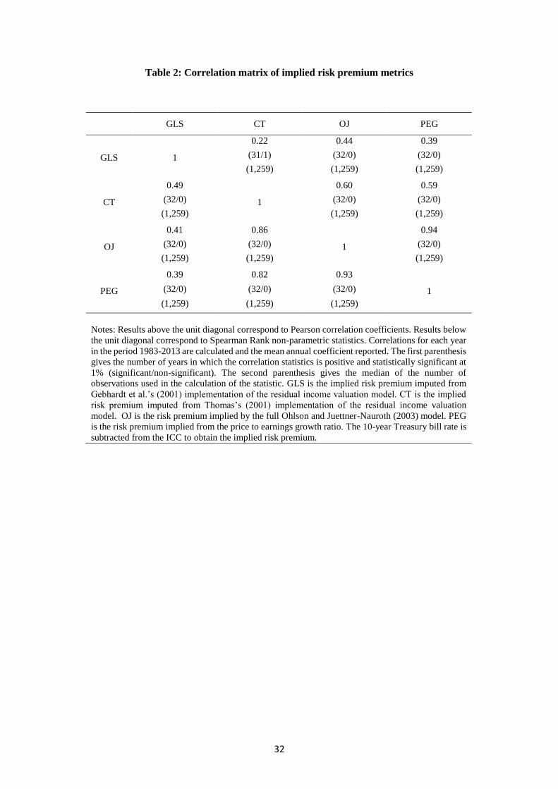
32

Table 2: Correlation matrix of implied risk premium metrics

GLS CT OJ PEG

GLS 1

0.22 0.44 0.39

(31/1) (32/0) (32/0)

(1,259) (1,259) (1,259)

CT

0.49

1

0.60 0.59

(32/0) (32/0) (32/0)

(1,259) (1,259) (1,259)

OJ

0.41 0.86

1

0.94

(32/0) (32/0) (32/0)

(1,259) (1,259) (1,259)

PEG

0.39 0.82 0.93

1 (32/0) (32/0) (32/0)

(1,259) (1,259) (1,259)

Notes: Results above the unit diagonal correspond to Pearson correlation coefficients. Results below

the unit diagonal correspond to Spearman Rank non-parametric statistics. Correlations for each year

in the period 1983-2013 are calculated and the mean annual coefficient reported. The first parenthesis

gives the number of years in which the correlation statistics is positive and statistically significant at

1% (significant/non-significant). The second parenthesis gives the median of the number of

observations used in the calculation of the statistic. GLS is the implied risk premium imputed from

Gebhardt et al.’s (2001) implementation of the residual income valuation model. CT is the implied

risk premium imputed from Thomas’s (2001) implementation of the residual income valuation

model. OJ is the risk premium implied by the full Ohlson and Juettner-Nauroth (2003) model. PEG

is the risk premium implied from the price to earnings growth ratio. The 10-year Treasury bill rate is

subtracted from the ICC to obtain the implied risk premium.

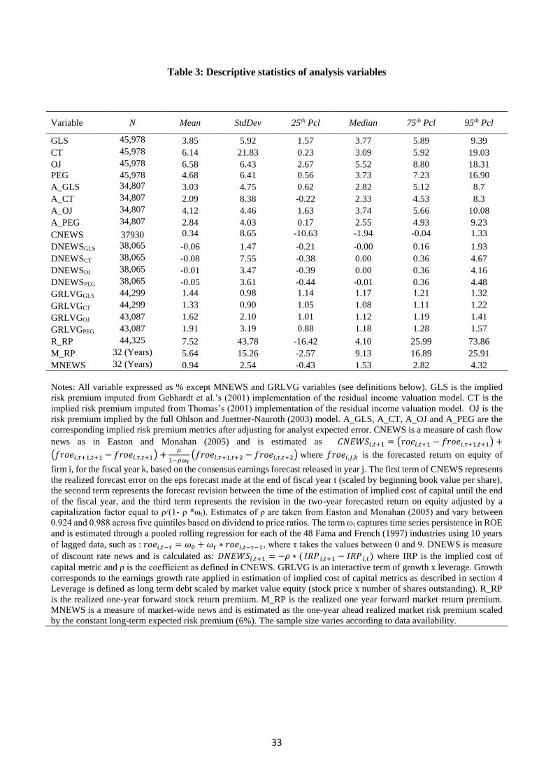
33

Table 3: Descriptive statistics of analysis variables

Variable N Mean StdDev 25th Pcl Median 75th Pcl 95th Pcl

GLS 45,978 3.85 5.92 1.57 3.77 5.89 9.39

CT 45,978 6.14 21.83 0.23 3.09 5.92 19.03

OJ 45,978 6.58 6.43 2.67 5.52 8.80 18.31

PEG 45,978 4.68 6.41 0.56 3.73 7.23 16.90

A_GLS 34,807 3.03 4.75 0.62 2.82 5.12 8.7

A_CT 34,807 2.09 8.38 -0.22 2.33 4.53 8.3

A_OJ 34,807 4.12 4.46 1.63 3.74 5.66 10.08

A_PEG 34,807 2.84 4.03 0.17 2.55 4.93 9.23

CNEWS 37930 0.34 8.65 -10.63 -1.94 -0.04 1.33

DNEWSGLS 38,065 -0.06 1.47 -0.21 -0.00 0.16 1.93

DNEWSCT 38,065 -0.08 7.55 -0.38 0.00 0.36 4.67

DNEWSOJ 38,065 -0.01 3.47 -0.39 0.00 0.36 4.16

DNEWSPEG 38,065 -0.05 3.61 -0.44 -0.01 0.36 4.48

GRLVGGLS 44,299 1.44 0.98 1.14 1.17 1.21 1.32

GRLVGCT 44,299 1.33 0.90 1.05 1.08 1.11 1.22

GRLVGOJ 43,087 1.62 2.10 1.01 1.12 1.19 1.41

GRLVGPEG 43,087 1.91 3.19 0.88 1.18 1.28 1.57

R_RP 44,325 7.52 43.78 -16.42 4.10 25.99 73.86

M_RP 32 (Years) 5.64 15.26 -2.57 9.13 16.89 25.91

MNEWS 32 (Years) 0.94 2.54 -0.43 1.53 2.82 4.32

Notes: All variable expressed as % except MNEWS and GRLVG variables (see definitions below). GLS is the implied

risk premium imputed from Gebhardt et al.’s (2001) implementation of the residual income valuation model. CT is the

implied risk premium imputed from Thomas’s (2001) implementation of the residual income valuation model. OJ is the

risk premium implied by the full Ohlson and Juettner-Nauroth (2003) model. A_GLS, A_CT, A_OJ and A_PEG are the

corresponding implied risk premium metrics after adjusting for analyst expected error. CNEWS is a measure of cash flow

news as in Easton and Monahan (2005) and is estimated as 𝐶𝑁𝐸𝑊𝑆𝑖,𝑡+1 = (𝑟𝑜𝑒𝑖,𝑡+1 − 𝑓𝑟𝑜𝑒𝑖,𝜏+1,𝑡+1) +

(𝑓𝑟𝑜𝑒𝑖,𝜏+1,𝑡+1 − 𝑓𝑟𝑜𝑒𝑖,𝜏,𝑡+1) +𝜌

1−𝜌𝜔𝑡(𝑓𝑟𝑜𝑒𝑖,𝜏+1,𝑡+2 − 𝑓𝑟𝑜𝑒𝑖,𝜏,𝑡+2) where 𝑓𝑟𝑜𝑒𝑖,𝑗,𝑘 is the forecasted return on equity of

firm i, for the fiscal year k, based on the consensus earnings forecast released in year j. The first term of CNEWS represents

the realized forecast error on the eps forecast made at the end of fiscal year t (scaled by beginning book value per share),

the second term represents the forecast revision between the time of the estimation of implied cost of capital until the end

of the fiscal year, and the third term represents the revision in the two-year forecasted return on equity adjusted by a

capitalization factor equal to ρ/(1- ρ *ωt). Estimates of ρ are taken from Easton and Monahan (2005) and vary between

0.924 and 0.988 across five quintiles based on dividend to price ratios. The term ωt captures time series persistence in ROE

and is estimated through a pooled rolling regression for each of the 48 Fama and French (1997) industries using 10 years

of lagged data, such as : 𝑟𝑜𝑒𝑖,𝑡−𝜏 = 𝜔0 + 𝜔𝑡 ∗ 𝑟𝑜𝑒𝑖,𝑡−𝜏−1, where τ takes the values between 0 and 9. DNEWS is measure

of discount rate news and is calculated as: 𝐷𝑁𝐸𝑊𝑆𝑖,𝑡+1 = −𝜌 ∗ ( 𝐼𝑅𝑃 𝑖,𝑡+1 − 𝐼𝑅𝑃 𝑖,𝑡) where IRP is the implied cost of

capital metric and ρ is the coefficient as defined in CNEWS. GRLVG is an interactive term of growth x leverage. Growth

corresponds to the earnings growth rate applied in estimation of implied cost of capital metrics as described in section 4

Leverage is defined as long term debt scaled by market value equity (stock price x number of shares outstanding). R_RP

is the realized one-year forward stock return premium. M_RP is the realized one year forward market return premium.

MNEWS is a measure of market-wide news and is estimated as the one-year ahead realized market risk premium scaled

by the constant long-term expected risk premium (6%). The sample size varies according to data availability.

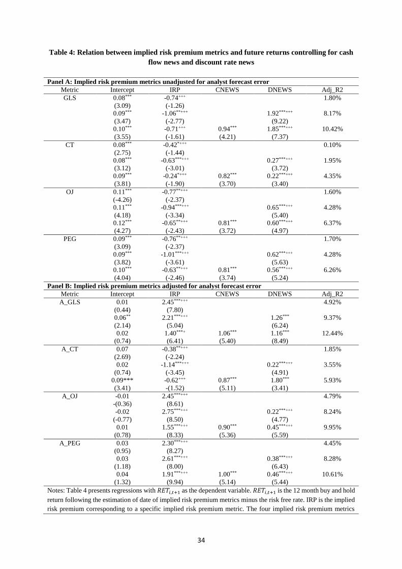
34

Table 4: Relation between implied risk premium metrics and future returns controlling for cash

flow news and discount rate news

Panel A: Implied risk premium metrics unadjusted for analyst forecast error Metric Intercept IRP CNEWS DNEWS Adj_R2

GLS 0.08*** -0.74+++ 1.80%

(3.09) (-1.26)

0.09*** -1.06**+++ 1.92***+++ 8.17%

(3.47) (-2.77) (9.22)

0.10*** -0.71+++ 0.94*** 1.85***+++ 10.42%

(3.55) (-1.61) (4.21) (7.37)

CT 0.08*** -0.42*+++ 0.10%

(2.75) (-1.44)

0.08*** -0.63***+++ 0.27***+++ 1.95%

(3.12) (-3.01) (3.72)

0.09*** -0.24*+++ 0.82*** 0.22***+++ 4.35%

(3.81) (-1.90) (3.70) (3.40)

OJ 0.11*** -0.77**+++ 1.60%

(-4.26) (-2.37)

0.11*** -0.94***+++ 0.65***+++ 4.28%

(4.18) (-3.34) (5.40)

0.12*** -0.65**+++ 0.81*** 0.60***+++ 6.37%

(4.27) (-2.43) (3.72) (4.97)

PEG 0.09*** -0.76**+++ 1.70%

(3.09) (-2.37)

0.09*** -1.01***+++ 0.62***+++ 4.28%

(3.82) (-3.61) (5.63)

0.10*** -0.63**+++ 0.81*** 0.56***+++ 6.26%

(4.04) (-2.46) (3.74) (5.24)

Panel B: Implied risk premium metrics adjusted for analyst forecast error

Metric Intercept IRP CNEWS DNEWS Adj_R2

A_GLS 0.01 2.45***+++ 4.92%

(0.44) (7.80)

0.06** 2.21***+++ 1.26*** 9.37%

(2.14) (5.04) (6.24)

0.02 1.40***+ 1.06*** 1.16*** 12.44%

(0.74) (6.41) (5.40) (8.49)

A_CT 0.07 -0.38**+++ 1.85%

(2.69) (-2.24)

0.02 -1.14***+++ 0.22***+++ 3.55%

(0.74) (-3.45) (4.91)

0.09*** -0.62+++ 0.87*** 1.80*** 5.93%

(3.41) -(1.52) (5.11) (3.41)

A_OJ -0.01 2.45***+++ 4.79%

-(0.36) (8.61)

-0.02 2.75***+++ 0.22***+++ 8.24%

(-0.77) (8.50) (4.77)

0.01 1.55***+++ 0.90*** 0.45***+++ 9.95%

(0.78) (8.33) (5.36) (5.59)

A_PEG 0.03 2.30***+++ 4.45%

(0.95) (8.27)

0.03 2.61***+++ 0.38***+++ 8.28%

(1.18) (8.00) (6.43)

0.04 1.91***+++ 1.00*** 0.46***+++ 10.61%

(1.32) (9.94) (5.14) (5.44)

Notes: Table 4 presents regressions with 𝑅𝐸𝑇𝑖,𝑡+1 as the dependent variable. 𝑅𝐸𝑇𝑖,𝑡+1 is the 12 month buy and hold

return following the estimation of date of implied risk premium metrics minus the risk free rate. IRP is the implied

risk premium corresponding to a specific implied risk premium metric. The four implied risk premium metrics

35

used (GLS, CT, OJ, PEG) are defined in section 4. PANEL A presents results using implied risk premium metrics

without adjustments for analyst expected error. CNEWS is a measure of cash flow news as in Easton and Monahan

(2005) and is estimated as 𝐶𝑁𝐸𝑊𝑆𝑖,𝑡+1 = (𝑟𝑜𝑒𝑖,𝑡+1 − 𝑓𝑟𝑜𝑒𝑖,𝜏+1,𝑡+1) + (𝑓𝑟𝑜𝑒𝑖,𝜏+1,𝑡+1 − 𝑓𝑟𝑜𝑒𝑖,𝜏,𝑡+1) +𝜌

1−𝜌𝜔𝑡(𝑓𝑟𝑜𝑒𝑖,𝜏+1,𝑡+2 − 𝑓𝑟𝑜𝑒𝑖,𝜏,𝑡+2) where 𝑓𝑟𝑜𝑒𝑖,𝑗,𝑘 is the forecasted return on equity of firm i, for the fiscal year k,

based on the consensus earnings forecast released in year j. The first term of CNEWS represents the realized

forecast error on the eps forecast made at the end of fiscal year t (scaled by beginning book value per share), the

second term represents the forecast revision between the time of the estimation of implied cost of capital until the

end of the fiscal year, and the third term represents the revision in the two-year forecasted return on equity adjusted

by a capitalization factor equal to ρ/(1- ρ *ωt). Estimates of ρ are taken from Easton and Monahan (2005) and vary

between 0.924 and 0.988 across five quintiles based on dividend to price ratios. The term ω t captures time series

persistence in ROE and is estimated through a pooled rolling regression for each of the 48 Fama and French (1997)

industries using 10 years of lagged data, such as: 𝑟𝑜𝑒𝑖,𝑡−𝜏 = 𝜔0 + 𝜔𝑡 ∗ 𝑟𝑜𝑒𝑖,𝑡−𝜏−1, where τ takes the values between

0 and 9. DNEWS is measure of discount rate news and is calculated as: 𝐷𝑁𝐸𝑊𝑆𝑖,𝑡+1 = −𝜌 ∗ ( 𝐼𝑅𝑃 𝑖,𝑡+1 − 𝐼𝑅𝑃 𝑖,𝑡)

where IRP is the implied cost of capital metric and ρ is the coefficient as defined in CNEWS. PANEL B presents

multivariate regressions using implied risk premium metrics adjusted for analyst expected error. Mean coefficients

for annual cross-sectional regressions are reported in all panels. T-statistics in parenthesis are based on Newey-

West standard errors. *** (**)(*) denotes statistical significance at 1% (5%) (10%) for tests of coefficients different

from zero. +++ (++) (+) denotes statistical significance at 1% (5%) (10%) for tests of coefficients different from one.

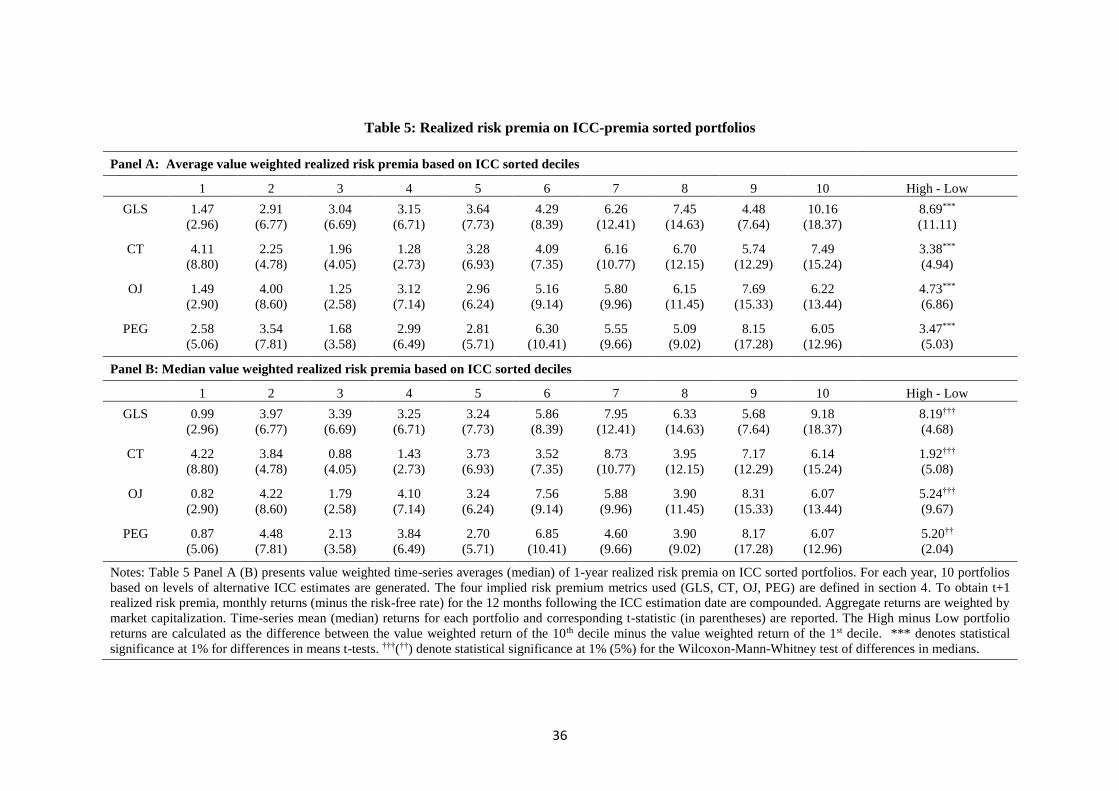
36

Table 5: Realized risk premia on ICC-premia sorted portfolios

Panel A: Average value weighted realized risk premia based on ICC sorted deciles

1 2 3 4 5 6 7 8 9 10 High - Low

GLS 1.47 2.91 3.04 3.15 3.64 4.29 6.26 7.45 4.48 10.16 8.69***

(2.96) (6.77) (6.69) (6.71) (7.73) (8.39) (12.41) (14.63) (7.64) (18.37) (11.11)

CT 4.11 2.25 1.96 1.28 3.28 4.09 6.16 6.70 5.74 7.49 3.38***

(8.80) (4.78) (4.05) (2.73) (6.93) (7.35) (10.77) (12.15) (12.29) (15.24) (4.94)

OJ 1.49 4.00 1.25 3.12 2.96 5.16 5.80 6.15 7.69 6.22 4.73***

(2.90) (8.60) (2.58) (7.14) (6.24) (9.14) (9.96) (11.45) (15.33) (13.44) (6.86)

PEG 2.58 3.54 1.68 2.99 2.81 6.30 5.55 5.09 8.15 6.05 3.47***

(5.06) (7.81) (3.58) (6.49) (5.71) (10.41) (9.66) (9.02) (17.28) (12.96) (5.03)

Panel B: Median value weighted realized risk premia based on ICC sorted deciles

1 2 3 4 5 6 7 8 9 10 High - Low

GLS 0.99 3.97 3.39 3.25 3.24 5.86 7.95 6.33 5.68 9.18 8.19†††

(2.96) (6.77) (6.69) (6.71) (7.73) (8.39) (12.41) (14.63) (7.64) (18.37) (4.68)

CT 4.22 3.84 0.88 1.43 3.73 3.52 8.73 3.95 7.17 6.14 1.92†††

(8.80) (4.78) (4.05) (2.73) (6.93) (7.35) (10.77) (12.15) (12.29) (15.24) (5.08)

OJ 0.82 4.22 1.79 4.10 3.24 7.56 5.88 3.90 8.31 6.07 5.24†††

(2.90) (8.60) (2.58) (7.14) (6.24) (9.14) (9.96) (11.45) (15.33) (13.44) (9.67)

PEG 0.87 4.48 2.13 3.84 2.70 6.85 4.60 3.90 8.17 6.07 5.20††

(5.06) (7.81) (3.58) (6.49) (5.71) (10.41) (9.66) (9.02) (17.28) (12.96) (2.04)

Notes: Table 5 Panel A (B) presents value weighted time-series averages (median) of 1-year realized risk premia on ICC sorted portfolios. For each year, 10 portfolios

based on levels of alternative ICC estimates are generated. The four implied risk premium metrics used (GLS, CT, OJ, PEG) are defined in section 4. To obtain t+1

realized risk premia, monthly returns (minus the risk-free rate) for the 12 months following the ICC estimation date are compounded. Aggregate returns are weighted by

market capitalization. Time-series mean (median) returns for each portfolio and corresponding t-statistic (in parentheses) are reported. The High minus Low portfolio

returns are calculated as the difference between the value weighted return of the 10th decile minus the value weighted return of the 1st decile. *** denotes statistical

significance at 1% for differences in means t-tests. †††(††) denote statistical significance at 1% (5%) for the Wilcoxon-Mann-Whitney test of differences in medians.

37

Table 6: Relation between implied risk premium metrics and future returns controlling for

market news, cash flow news, discount rate news and growth x leverage

Panel A: Implied risk premium metrics unadjusted for analyst forecast error

Metric Intercept MIRP CNEWS DNEWS GRLVG Adj_R2

GLS 0.07*** 0.57**++ 2.98%

(3.50) (2.69)

0.07*** 0.53**++ 1.68***++ 9.32%

(3.07) (2.33) (6.42)

0.08*** 0.33*+++ 1.01*** 1.78***+++ 12.0%

(3.96) (1.66) (5.25) (11.22)

0.05** 0.60***+ 1.03*** 1.84***+++ 0.015 14.5%

(2.11) (3.21) (5.33) (5.33) (1.17)

CT 0.06*** 0.14+++ 1.51%

(2.87) (1.30)

0.06*** 0.18+++ 0.24***+++ 2.89%

(2.35) (1.34) (4.41)

0.07*** 0.22**+++ 0.864*** 0.25**+++ 6.91%

(2.88) (2.24) (5.49) (4.93)

0.04 0.22**+++ 0.85*** 0.25***+++ 0.02 7.76%

(1.39) (2.29) (5.53) (4.92) (1.33)

OJ 0.09*** 0.17+++ 2.27%

(4.09) (1.26)

0.09*** 0.23+++ 0.57***+++ 5.54%

(3.67) (1.54) (3.67)

0.10*** 0.29**+++ 0.88*** 0.54***+++ 7.78%

(4.30) (2.36) (4.58) (7.05)

0.08*** 0.31**+++ 0.88*** 0.57***+++ 0.01 8.85%

(3.40) (2.48) (4.68) (7.68) (0.99)

PEG 0.08*** 0.22*+++ 2.16%

(3.69) (1.84)

0.07*** 0.29*+++ 0.54***+++ 5.44%

(2.81) (1.75) (5.43)

0.08*** 0.37**+++ 0.87*** 0.56***+++ 8.76%

(4.63) (2.29) (4.63) (4.63)

0.06*** 0.38**+++ 0.87*** 0.54***+++ 0.01 9.09%

(2.82) (2.22) (4.70) (5.97) (1.52)

Panel B: Implied risk premium metrics adjusted for analyst forecast error

Metric Intercept MIRP CNEWS DNEWS GRLVG Adj_R2

GLS 0.04 0.51**++ 5.34%

(1.57) (2.45)

0.09*** 1.19*** 1.36*** 10.5%

(6.22) (4.15) (6.22)

0.06** 1.52*** 1.65***++ 1.51***++ 16.42%

(2.69) (3.60) (5.25) (6.91)

0.05** 1.14*** 1.44*** 1.26***+ -0.04 14.89%

(2.07) (3.81) (5.39) (8.42) (-0.34)

CT 0.07*** 0.05 3.89%

(2.83) (0.18)

0.00 0.58***+ 0.23***+++ 5.74%

(0.04) (2.80) (5.06)

0.03 0.62***+ 0.90*** 0.01***+++ 10.21%

(1.44) (2.89) (6.30) (4.56)

-0.02 0.63*** + 0.89*** 0.20***+++ 0.04** 10.9%

(-0.59) (2.95) (8.19) (4.28) (2.23)

OJ 0.04 0.86*** 5.77%

(1.50) (4.07)

38

0.05** 1.19*** 0.49***+++ 8.37%

(2.32) (5.21) (5.66)

0.04* 1.19*** 1.04*** 0.54***+++ 12.53%

(1.88) (4.42) (4.95) (5.75)

0.03 1.07*** 1.05*** 0.58***+++ 0.01** 12.61%

(1.38) (4.22) (4.79) (6.79) (2.54)

PEG 0.05* 0.67** 5.14%

(2.03) (2.71)

0.07** 1.38*** 0.44***+++ 7.95%

(2.88) (5.03) (6.33)

0.06** 0.78** 1.07*** 0.52***+++ 11.74%

(2.58) (2.73) (4.71) (5.64)

0.05* 0.82*** 1.12*** 0.55***+++ 0.01*** 12.3%

(2.01) (2.83) (4.77) (6.59) (2.83)

Panel C: Implied risk premium metrics adjusted for analyst forecast error - CNEWS* excludes

market news effect

Metric Intercept MIRP CNEWS* DNEWS GRLVG Adj_R2

GLS 0.09*** 1.25*** 2.37***+++ 1.61***++ -0.03** 18.97%

(3.47) (4.70) (6.11) (7.13) (-2.15)

CT 0.02 0.49**+++ 1.70***+++ 0.25**+++ 0.01 13.08%

(1.25) (2.48) (9.49) (2.47) (1.11)

OJ -0.02 1.18*** 1.75***+++ 0.60***+++ 0.01*** 20.47%

(-1.04) (5.82) (8.46) (6.75) (3.86)

PEG 0.06** 1.02*** 1.99***+++ 0.52***+++ 0.00*** 14.69%

(2.34) (4.24) (5.72) (6.89) (2.99)

Notes: Table 6 presents regressions with 𝑅𝐸𝑇𝑖,𝑡+1 as the dependent variable. 𝑅𝐸𝑇𝑖,𝑡+1 is the 12 month buy and hold

return following the estimation of date of implied risk premium metrics minus the risk free rate. IRP is the implied risk

premium corresponding to a specific implied risk premium metric. The four implied risk premium metrics used (GLS,

CT, OJ, PEG) are defined in section 4. Panel A presents results using implied risk premium metrics without adjustments

for analyst expected error. Panel B presents multivariate regressions using implied risk premium metrics adjusted for

analyst expected error. MNEWS is a measure of market-wide news and is estimated as the one-year ahead realized

market risk premium scaled by the constant long-term expected risk premium (6%). CNEWS is a measure of cash flow

news as in Easton and Monahan (2005) and is estimated as: 𝐶𝑁𝐸𝑊𝑆𝑡+1 = (𝑟𝑜𝑒𝑡+1 − 𝑓𝑟𝑜𝑒𝜏+1,𝑡+1) + (𝑓𝑟𝑜𝑒𝜏+1,𝑡+1 −

𝑓𝑟𝑜𝑒𝜏,𝑡+1) +𝜌

1−𝜌𝜔𝑡(𝑓𝑟𝑜𝑒𝜏+1,𝑡+2 − 𝑓𝑟𝑜𝑒𝜏,𝑡+2) where froeij,k is the forecasted return on equity of firm i, for the fiscal

year k, based on the consensus earnings forecast released in year j. The first term of CNEWS represents the realized

forecast error on the eps forecast made at the end of fiscal year t (scaled by beginning book value per share), the second

term represents the forecast revision between the time of the estimation of implied cost of capital until the end of the

fiscal year, and the third term represents the revision in the two-year forecasted return on equity adjusted by a

capitalization factor equal to ρ/(1- ρ *ωt). Estimates of ρ are taken from Easton and Monahan (2005) and vary between

0.924 and 0.988 across five quintiles based on dividend to price ratios. The term ωt captures time series persistence in

ROE and is estimated through a pooled rolling regression for each of the 48 Fama and French (1997) industries using

10 years of lagged data, such as: 𝑟𝑜𝑒𝑖,𝑡−𝜏 = 𝜔0 + 𝜔𝑡 ∗ 𝑟𝑜𝑒𝑖,𝑡−𝜏−1, where τ takes the values between 0 and 9. DNEWS

is measure of discount rate news and is calculated as: 𝐷𝑁𝐸𝑊𝑆𝑖,𝑡+1 = −𝜌 ∗ ( 𝐼𝑅𝑃 𝑖,𝑡+1 − 𝐼𝑅𝑃 𝑖,𝑡) where IRP is the

implied cost of capital metric and ρ is the coefficient as defined in CNEWS. GRLVG is an interactive term of growth

x leverage. Growth corresponds to the earnings growth rate applied in estimation of implied cost of capital metrics as

described in section 4 Leverage is defined as long term debt scaled by market value equity (stock price x number of

shares outstanding). Panel C presents results for implied risk premium metrics adjusted for analyst expected error where

CNEWS* is the residual from a first-pass regression of CNEWS on (𝑀𝑁𝐸𝑊𝑆𝑡+1 − 1)𝐼𝑅𝑃𝑖,𝑡. Mean coefficients for

annual cross-sectional regressions are reported in all panels. T-statistics in parenthesis are based on Newey-West

standard errors. *** (**)(*) denotes statistical significance at 1% (5%) (10%) for tests of coefficients different from

zero. +++ (++) (+) denotes statistical significance at 1% (5%) (10%) for tests of coefficients different from one.

39

Table 7: Estimated mean reversion of implied cost of capital metrics based on AR1 model for

1,133 firms with 10 or more observations for period 1983-2013

Panel A: Summary results from time series regression model 𝑰𝑪𝑪𝒊,𝒕+𝟏 = 𝒂𝟎 + 𝒂𝟏𝑰𝑪𝑪𝒊,𝒕 + 𝒆𝒕+𝟏

Metric Intercept (�̂�0) Slope (�̂�1) �̂� = �̂�0/(1 − �̂�1)

GLS Mean estimate 0.07 0.14 0.08

Median estimate 0.07 0.10 0.08+++

No. pos. @ 10% level 1,034*** 237***

CT Mean estimate 0.06 0.15 0.007

Median estimate 0.06 0.14 0.07+++

No.pos.@10% level 1,007*** 386***

OJ Mean estimate 0.08 0.05 0.09

Median estimate 0.08 0.05 0.09+++

No.pos.@10% level 1,083*** 283***

PEG Mean estimate 0.07 0.05 0.08

Median estimate 0.07 0.03 0.08+++

No.pos.@10% level 1,069*** 286***

Panel B: Cross-firm distributional statistics for �̂�𝟎, �̂�𝟏, and �̂�

Metric Mean Stdv 5 Pcl 25 Pcl 50 Pcl 75 Pcl 95Pcl

GLS �̂�0 0.07 0.03 0.02 0.05 0.07 0.09 0.12

�̂�1 0.14 0.39 -0.39 -.0.09 0.10 0.38 0.76

�̂� 0.08 0.04 0.05 0.07 0.08 0.09 0.11

CT �̂�0 0.06 0.03 0.02 0.04 0.06 0.08 0.11

�̂�1 0.15 0.38 -0.45 -0.10 0.14 0.39 0.77

�̂� 0.07 0.03 0.04 0.06 0.07 0.08 0.11

OJ �̂�0 0.08 0.04 0.03 0.06 0.08 0.10 0.15

�̂�1 0.05 0.35 -0.52 -0.15 0.05 0.27 0.60

�̂� 0.09 0.03 0.06 0.08 0.09 0.10 0.12

PEG �̂�0 0.07 0.03 0.02 0.05 0.07 0.09 0.12

�̂�1 0.05 0.36 -0.48 -0.18 0.03 0.26 0.69

�̂� 0.08 0.25 0.05 0.06 0.08 0.09 0.11

Notes: Panel A presents results of AR(1) firm-specific regressions for alternative implied cost of capital

metrics (GLS, CT, OJ, PEG) as defined in section 4. Maximum likelihood estimates correcting for first

order autocorrelation of residuals are reported. ‘No.pos.@10% level’ denotes the number of firm

coefficients which are significantly positive at the 10% level. *** indicates that the number of significant

coefficients is above that expected by chance at the 1% level based on a binomial test (for our sample

of 1133 firms, the number of significant coefficients must exceed 137 based on a 1% binomial test). +++ denotes significance of the median of �̂� for a particular ICC at the 1% level based on the Mann-

Whitney-Wilcoxon test. Panel B presents distributional statistics for �̂�0, �̂�1, and �̂� based on 1,133 firm

estimates for the alternative ICC metrics.

40

Table 8: Time-series regressions of realized return on implied risk premia for 1,133 firms with

10 or more observations for period 1983-2013

Panel A: Results for model 𝑹𝑬𝑻𝒊,𝒕+𝟏 = 𝒃𝟎 + 𝒃𝟏𝑰𝑹𝑷𝒊,𝒕+𝒆𝒕+𝟏

Metric �̂�𝟎 �̂�𝟏 Mean Adj. R2

GLS Mean estimate 0.01 2.60 11.01%

Median estimate 0.04 1.82

No. pos. @ 10% level 175*** 285***

No. 𝑏1 ≠ 1 @ 10% level 158***

CT Mean estimate 0.12 -1.57 9.34%

Median estimate 0.10 -1.18

No. pos. @ 10% level 414*** 78

No. 𝑏1 ≠ 1 @ 10% level 195***

OJ Mean estimate 0.01 2.24 11.12%

Median estimate 0.03 1.69

No. pos. @ 10% level 159*** 286***

No. 𝑏1 ≠ 1 @ 10% level 149***

PEG Mean estimate 0.04 1.87 10.36%

Median estimate 0.05 1.31

No. pos. @ 10% level 242*** 239***

No. 𝑏1 ≠ 1 @ 10% level 144***

Panel B: Results for model 𝑹𝑬𝑻𝒊,𝒕+𝟏 = 𝒃𝟎 + 𝒃𝟏𝑴𝑰𝑹𝑷𝒊,𝒕+𝒆𝒕+𝟏

�̂�𝟎 �̂�𝟏 Mean Adj. R2

GLS Mean estimate 0.07 0.83 19.44%

Median estimate 0.06 0.84

No. pos. @ 10% level 321*** 534***

No. 𝑏1 ≠ 1 @ 10% level 216***

CT Mean estimate 0.09 0.18 13.04%

Median estimate 0.07 0.44

No. pos. @ 10% level 376*** 282***

No. 𝑏1 ≠ 1 @ 10% level 250***

OJ Mean estimate 0.06 0.95 20.57%

Median estimate 0.05 0.84

No. pos. @ 10% level 305*** 605***

No. 𝑏1 ≠ 1 @ 10% level 209***

PEG Mean estimate 0.07 0.84 18.17%

Median estimate 0.06 0.85

No. pos. @ 10% level 340*** 509***

No. 𝑏1 ≠ 1 @ 10% level 206***

Notes: Panel A presents results from firm-specific regressions of realized risk premium against implied

risk premia (IRP) for alternative ICC metrics (GLS, CT, OJ, PEG) as defined in section 4. Panel B

presents results from firm specific regressions of realized risk premium against implied risk premia

adjusted for market news (MIRP) for alternative ICC metrics. ‘No. pos. @ 10% level’ denotes the number

of firm coefficients which are significantly positive at the 10% level. ‘No. 𝑏1 ≠ 1 @ 10% level’ denotes

the number of firms with significant t-statistics at the 10% level based on the alternative null hypothesis

that 𝑏1 ≠ 1.*** indicates that the number of significant coefficients is above that expected by chance at

the 1% level based on a binomial test (for our sample of 1133 firms, the number of significant coefficients

must exceed 137 based on a 1% binomial test).

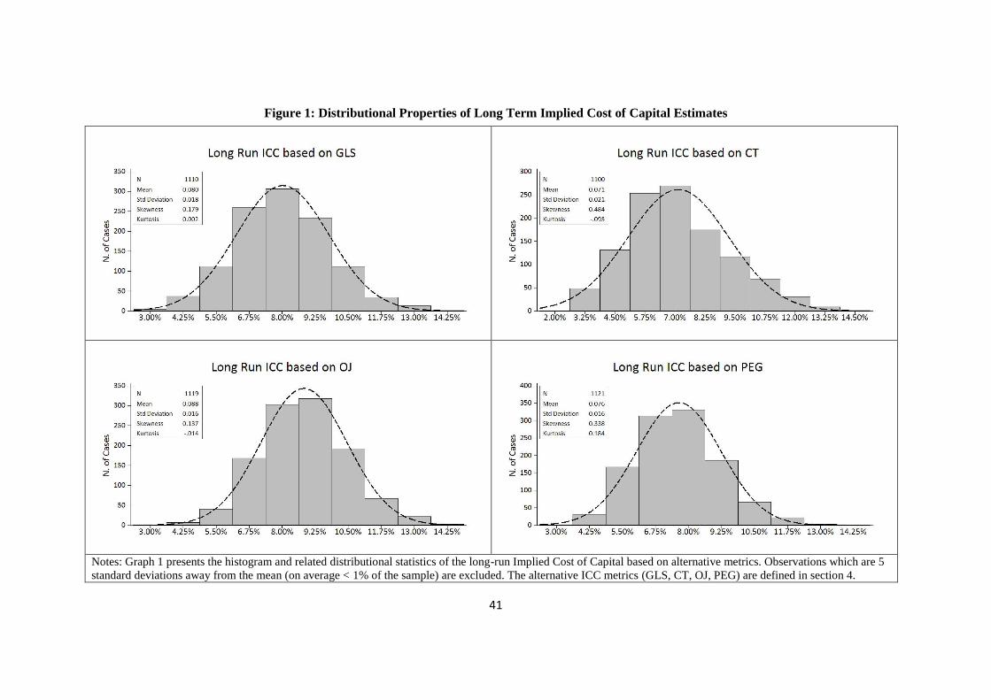
41

Figure 1: Distributional Properties of Long Term Implied Cost of Capital Estimates

Notes: Graph 1 presents the histogram and related distributional statistics of the long-run Implied Cost of Capital based on alternative metrics. Observations which are 5

standard deviations away from the mean (on average < 1% of the sample) are excluded. The alternative ICC metrics (GLS, CT, OJ, PEG) are defined in section 4.

42

Appendix A: A simple analysis where MNEWS and CNEWS are separate explanatory variables

for realized returns

In section 3.4, we consider the cases where (i) MNEWS is subsumed within CNEWS and

DNEWS and (ii) MNEWS is incremental to CNEWS and DNEWS. Given that the original theoretical

analysis of Vuolteenaho (2002) assumes the first case where all information for explaining realized stock

returns is subsumed within CNEWS and DNEWS (as indicated in our equation (6)), it is useful to

consider possible conditions under which implementation of the Vuolteenaho (2002) analysis implies

the second case where MNEWS has an incremental role beyond CNEWS and DNEWS. In the spirit of

Campbell and Vuolteenaho (2004) and Campbell et al (2009) where overall beta risk is broken down to

highlight systematic ‘cash flow’ and ‘discount rate’ risk, we present a simple model of ‘cash flow’ risk

where firms’ accounting returns co-vary with overall stock market returns. Specifically, we assume a

forecast model for ROE based on a random walk adjusted for market returns and show that if analysts’

ROE forecasts are based on accurate predictions of realized market returns, then CNEWS (measured

relative to their forecasts) will exclude MNEWS. This in turns implies the need to add MNEWS to

CNEWS and DNEWS (and the expected stock return for a firm) to obtain the realized stock return for

the firm.

First, we present our simple analysis based on a specific implementation of equation (7) in

section 3.2. We focus on the relationship between realized returns and expected returns as this is our

primary concern here (and simply ignore the issue of the ICC as an estimator of expected returns).

Second, we provide a brief interpretation of the role of CNEWS and MNEWS in the model.

i. Analysis based on simple ROE forecast model

All variables are as defined in the main text. We assume ROE for firm i is based on a time-

series model where realized (excess) market returns are related to the change in ROE as follows:

𝛥𝑥𝑖𝑡+1 = 𝛾𝑖𝜆𝑡+1 + 𝑢𝑖𝑡+1 (A1)

where 𝑢𝑖𝑡+1 is a mean zero shock. The forecast of 𝛥𝑥𝑖𝑡+1 as at date t is therefore:

𝑓𝑡(𝛥𝑥𝑖𝑡+1) = 𝛾𝑖𝜆 (A2)

and hence the earnings forecast error at date t+1 is:

𝑢𝑖𝑡+1+𝛾𝑖(𝜆𝑡+1 − 𝜆 ) = (𝛥𝑥𝑖𝑡+1 − 𝛾𝑖𝜆𝑡+1)+𝛾𝑖(𝜆𝑡+1 − 𝜆 ) = 𝛥𝑥𝑖𝑡+1−𝛾𝑖𝜆 (A3)

Noting that the earnings forecast error is expected to persist indefinitely given the time series process

represented by (A1), we make use of (A3) in equation (7) to obtain the following relationship between

realised stock returns and expected returns as follows:

𝑟𝑖𝑡+1∗ = 𝜇𝑖𝑡

∗𝑡+1 +1

(1 − 𝜌)(𝛥𝑥𝑖𝑡+1 − 𝛾𝑖𝜆) − 𝜌(𝜇𝑖𝑡+1

𝑡+2 − 𝜇𝑖) (A4)

Using the second element of (A3) in equation (A4) and re-arranging gives:

𝑟𝑖𝑡+1∗ = (𝜇𝑖𝑡

∗𝑡+1 +𝛾𝑖

(1 − 𝜌)(𝜆𝑡+1 − 𝜆 )) +

1

(1 − 𝜌)(𝛥𝑥𝑖𝑡+1 − 𝛾𝑖𝜆𝑡+1) − 𝜌(𝜇𝑖𝑡+1

𝑡+2 − 𝜇𝑖) (A5)

43

which in turn implies:

𝑟𝑖𝑡+1∗ =

𝜆𝑡+1

𝜆𝜇𝑖

∗ +1

(1 − 𝜌)(𝛥𝑥𝑖𝑡+1 − 𝛾𝑖𝜆𝑡+1) − 𝜌(𝜇𝑖𝑡+1

𝑡+2 − 𝜇𝑖) (A6)

for the special case where 𝜇𝑖𝑡∗𝑡+1 = 𝜇𝑖

∗ and 𝛾𝑖 = 𝜇𝑖∗(1 − 𝜌) 𝜆⁄ = 𝛽𝑖(1 − 𝜌). In summary, for the special

case of the ROE forecast model represented by (A1) where 𝛾𝑖 = 𝜇𝑖∗(1 − 𝜌) 𝜆⁄ = 𝛽𝑖(1 − 𝜌), it follows

from (A6) that MNEWS given by (𝜆𝑡+1

𝜆− 1) 𝜇𝑖

∗ is incremental to CNEWS (conditioned on 𝜆𝑡+1) and

DNEWS when explaining realised stock returns.10

ii. Interpretation

The analysis represented by equations (A1) to (A6) provides a simple setting to illustrate how

market news adjustment of expected returns may be beneficial in the presence of CNEWS and DNEWS

estimates. Specifically, if analysts are able to make accurate forecasts of overall market returns and

incorporate this knowledge into their estimates of future ROE, estimates of CNEWS will be entirely

firm specific and will exclude the impact of MNEWS on stock returns. Given analyst expertise and

understanding of the market’s within which different firms operate, it seems reasonable to assume that

they will be well-informed about the likely impact of market movements on the ROE performance of

firms which they follow. In terms of our simple analysis above represented by (A6), we therefore suggest

that analysts may have superior expectations of 𝛾𝑖𝜆𝑡+1 than market investors as a whole at the beginning

of period t+1 (who, according to our analysis, expect 𝛾𝑖𝜆𝑡+1 to equal 𝛾𝑖𝜆 at this time). While this

interpretation implies some semi-strong form capital market inefficiency (as investors should be able to

obtain analysts’ estimates of 𝛾𝑖𝜆𝑡+1 from their ROE forecasts), in a more complex setting than that

assumed by equations (A1)-(A6), it may be more difficult for investors to accurately gauge analysts’

market expectations. 11 Furthermore, our characterisation of market news as the interaction of a firm’s

beta (i.e., 𝛾𝑖 = 𝛽𝑖(1 − 𝜌) in (A6)) with the return on the excess return on the market as a whole, 𝜆𝑡+1,

is intended to serve as a simple and tractable representation of a more complex reality where analysts

are able to use their expert knowledge of different business sectors to accurately forecast movements in

a firm’s particular market sector (i.e., we have assumed that this knowledge can be approximated by

10 This special case can be viewed as a case where the overall return beta for firm i is equal to a measure of its

‘cash flow beta’. To see this, note that substituting 𝛾𝑖 = 𝛽𝑖(1 − 𝜌) in (A1) gives 𝛥𝑥𝑖𝑡+1 = 𝛽𝑖(1 − 𝜌)𝜆𝑡+1 + 𝑢𝑖𝑡+1.

This implies that:

𝛽𝑖 =𝑐𝑜𝑣[(1 − 𝜌)𝜆𝑡+1, 𝛥𝑥𝑖𝑡+1]

𝑣𝑎𝑟[(1 − 𝜌)𝜆𝑡+1]=

𝑐𝑜𝑣[𝜆𝑡+1, (1 − 𝜌)−1𝛥𝑥𝑖𝑡+1]

𝑣𝑎𝑟[𝜆𝑡+1]

The overall beta for firm i in this case therefore corresponds to ‘cash flow’ beta equal to the covariance of market

returns with unconditional cash flow news divided by the variance of the market. Correspondingly, given the

additivity property of cash flow and discount rate betas (Campbell et al., 2009), the discount rate beta for this

special case is zero (i.e., any discount rate news is assumed to be uncorrelated with the market). 11 Our argument that analysts are superior forecasters of the impact of market movements on firm performance is

broadly consistent with previous research such as Piotroski and Roulstone (2004) who show increased stock return

synchronicity associated with analyst activity. Our analysis, however, suggests that stock prices do not

immediately reflect the superior market forecasts of analysts which then leads to an incremental explanatory role

for MNEWS in explaining realised returns.

44

the interaction of the firm’s systematic risk and the return on the overall market). In summary, we suspect

that analysts’ ROE expectations may contain superior forecasts of market movements than those of

investors as a whole and that this will correspondingly result in the incremental role of MNEWS beyond

analyst based estimates of CNEWS as an explanatory variable for realised stock returns.

iii. Empirical implications

If market news is driven by changes in cash flow expectations, then empirical analysis based on

the following cross-sectional regression model (see section 4 for variable definitions) would be justified

if our measure of 𝐶𝑁𝐸𝑊𝑆𝑖,𝑡+1 based on analysts’ forecasts excludes market news (where market news

for any firm i is given by (𝑀𝑁𝐸𝑊𝑆𝑡+1 − 1)𝐼𝑅𝑃𝑖,𝑡 ):

𝑅𝐸𝑇𝑖,𝑡+1 = 𝜑0 + 𝜑1𝑀𝐼𝑅𝑃𝑖,𝑡 + 𝜑2𝐷𝑁𝐸𝑊𝑆𝑖,𝑡+1 + 𝜑3𝐶𝑁𝐸𝑊𝑆𝑖,𝑡+1 +𝜀𝑖,𝑡+1 (A7)

In this case, our analysis suggests an intercept 𝜑0=0 and slope coefficients 𝜑1 = 𝜑2 = 𝜑3 = 1. If, on

the other hand, the assumption that analysts’ forecasts exclude market news is incorrect i.e., if cash flow

news based on analysts’ forecasts contains market news, our analysis in section 3.4 suggests that the

market news adjustment will be reversed so that 𝜑1 = 1 𝑀𝑁𝐸𝑊𝑆𝑡+1⁄ , with other coefficients

unchanged. Our empirical results tend to support the former interpretation with 𝜑1 greater than zero but

generally not statistically distinguishable from 1. Furthermore, if 𝑀𝐼𝑅𝑃𝑖,𝑡 in equation (A7) is replaced

with 𝐼𝑅𝑃𝑖,𝑡, our results show that the estimated coefficient for 𝐼𝑅𝑃𝑖,𝑡 is generally statistically greater

than 1 which is consistent with 𝑀𝑁𝐸𝑊𝑆𝑡+1 > 1 (as indicated by the sample median 𝑀𝑁𝐸𝑊𝑆𝑡+1 of

1.527 reported in Table 3) and our measure of 𝐶𝑁𝐸𝑊𝑆𝑖,𝑡+1 not fully reflecting market news.

Finally, while we have argued that the relevance of market news beyond cash flow news for

stock returns may be due to analysts’ superior ability to forecast market news, it could also be due to

poor ability of analysts to fully incorporate implications of market news into revisions of future profit

forecasts or simply due to noise in our measures of 𝐶𝑁𝐸𝑊𝑆𝑖,𝑡+1 or 𝐷𝑁𝐸𝑊𝑆𝑖,𝑡+1which may obscure the

impact of changes in market expectations on these news variables. Based on the latter possibility, if we

assume market news is contained within a noisy measure of 𝐶𝑁𝐸𝑊𝑆𝑖,𝑡+1, the following regression

model which excludes market news from cash flow news is more appropriate than (A7) as it avoids a

‘double-counting’ of market news and is based on a cleaner measure of firm-specific cash flow news:

𝑅𝐸𝑇𝑖,𝑡+1 = 𝜑0 + 𝜑1𝑀𝐼𝑅𝑃𝑖,𝑡 + 𝜑2𝐷𝑁𝐸𝑊𝑆𝑖,𝑡+1 + 𝜑3𝐶𝑁𝐸𝑊𝑆𝑖,𝑡+1∗ +𝜀𝑖,𝑡+1 (A8)

where 𝐶𝑁𝐸𝑊𝑆𝑖,𝑡+1∗ is a measure of firm-specific cash flow news which is orthogonal to the market news

for firm i represented by (𝑀𝑁𝐸𝑊𝑆𝑡+1 − 1)𝐼𝑅𝑃𝑖,𝑡 (in our empirical analysis, we measure 𝐶𝑁𝐸𝑊𝑆𝑖,𝑡+1∗

for firm i in year t+1 as the residual from a cross-sectional regression of 𝐶𝑁𝐸𝑊𝑆𝑖,𝑡+1 on

(𝑀𝑁𝐸𝑊𝑆𝑡+1 − 1)𝐼𝑅𝑃𝑖,𝑡 for that year). In summary, if 𝐶𝑁𝐸𝑊𝑆𝑖,𝑡+1 contains market news but is a noisy

measure of overall cash flow news, we would expect a regression based on equation (A8) (where the

unnecessary inclusion of market news has been eliminated from cash flow news) to provide a better

explanation of realised stock returns than (A7).

45

Appendix B: Estimating Analysts’ Expected Errors

Following Larocque (2013) we model expected analyst error in eps1 and eps2 earnings’ forecasts by

estimating, respectively the following two specifications:

tjtjtjtjtojt EZRETaMVaLAGRETaErroraaError _)ln(_ 43211 (B1)

11432111 _)ln(_ tjtjtjtjtojt EZRETaMVaLAGRETaErroraaError (B2)

where :

tError

1

t

tt

P

AepsFeps

1tError

1

11

t

tt

P

AepsFeps

tFeps Median EPS forecast for year t according to the I/B/E/S summary report released

during April of year t.

1tFeps Median EPS forecast for year t+1 according to the I/B/E/S summary report released

during April of year t.

tAeps Actual earnings per share in year t according to I/B/E/S.

1tAeps Actual earnings per share in year t+1 according to I/B/E/S.

tLAGRET _ Total return to shareholders minus the value-weighted return on a market portfolio

from CRSP for the 12 months preceding the release of the April summary report.

)ln( tMV Natural Log of Market Value.

tEZRET _ The total return to shareholders minus the value-weighted return on a market

portfolio from CRSP from the day following the release of the April summary

report through to the day preceding the release of earnings for year t.

1_ tEZRET The total return to shareholders minus the value-weighted return on a market

portfolio from CRSP from the day following the release of the April summary

report through to the day preceding the release of earnings for year t+1..

We estimate the following coefficients for specifications (B1) and (B2). Our results are qualitative

identical to those of Larocque (2013). The table below presents the average coefficients and

corresponding t-stats.

Variable Intercept Errorjt-1 Ret_Lagjt LN(MVjt) RET_EZjt Adj. R2

Errorjt 0.019*** 0.235** -0.002*** -0.012*** -0.027*** 17.2%

(t-value) (7.64) (2.73) (-7.00) (-8.72) (-7.59)

Intercept Errorjt-1 Ret_Lagjt LN(MVjt) RET_EZjt+1 Adj. R2

Errorjt+1 0.047*** 0.453*** -0.010*** -0.005*** -0.040*** 20%

(t-value) (10.82) (2.91) (-3.24) (-11.74) (-8.74)

46

Appendix C: Underlying analysis for time-series regression models

In section 4.4.2, we present three empirical time series regression models, equations (13)-(15). This

appendix provides the underlying analysis which motivates each of these models. All variables are as

defined in section 3.

i. Equation (13)

The rationale for equation (13) is based on the assumption that the time series of expected returns may

be expressed as an AR1 process as follows:

𝜇𝑡𝑡+1 = 𝜑0 + 𝜑1𝜇𝑡−1

𝑡 + 𝑒1𝑡 (C1)

where 𝑒1𝑡 is a mean zero disturbance term. Our analytical framework assumes for simplicity that 𝜑1 =

0, so that the average expected return, 𝜇, is simply equal to 𝜑0. More generally, however, mean reversion

to a positive average expected return only requires 𝜑0 > 0 and 0 ≤ 𝜑1 < 1, where 𝜇 = 𝜑0 (1 − 𝜑1)⁄ .

Equation (C1) can therefore be re-written as:

𝜇𝑡𝑡+1 = 𝜇(1 − 𝜑1) + 𝜑1𝜇𝑡−1

𝑡 + 𝑒1𝑡 (C2)

In the spirit of Hughes et al (2009), we next assume that the implied cost of capital measures expected

return with error as follows:

𝜋𝑡 = 𝜑3 + 𝜇𝑡𝑡+1 + 𝑒2𝑡 (C3)

where 𝜑3 is the mean bias of the ICC and 𝑒2𝑡 is a mean zero disturbance term. Using (C3) in (C2) generates

the following time-series process for the implied cost of capital:

𝜋𝑡 = (𝜇 + 𝜑3)(1 − 𝜑1) + 𝜑1𝜋𝑡−1 + (𝑒1𝑡 + 𝑒2𝑡 − 𝜑1𝑒2𝑡−1) (C4)

Comparing equation (13) with (C4) confirms that the long-run mean ICC estimate, 𝑎0 (1 − 𝑎1)⁄ , may

be interpreted as an estimate of the sum of the average expected return and the mean bias of the ICC as

an estimator of expected returns, (𝜇 + 𝜑3). From an empirical point of view, equation (C4) also suggests

that estimation of equation (13) may be affected by negative autocorrelation in the residuals. This

implies that equation (13) should be estimated using a maximum likelihood procedure (rather than OLS)

due to the lagged dependent variable in equation (13).

ii. Equation (14)

Combining equation (5) in section 3 with (C3) above expressed as a deviation from the risk-free rate

i.e., 𝜋𝑡∗ = 𝜑3 + 𝜇𝑡

𝑡+1∗ + 𝑒2𝑡, gives:

𝑟𝑡+1∗ =

𝜆𝑡+1

𝜆𝜋𝑡

∗ + (𝜑3 + 𝑒2𝑡) (−𝜆𝑡+1

𝜆) + 𝜖𝑡+1 (C5)

The first variable, 𝜆𝑡+1

𝜆𝜋𝑡

∗, in (C5), corresponding to the empirical variable 𝑀𝐼𝑅𝑃𝑡, has a theoretical

regression coefficient of 1 and would be clearly be the sole explanatory variable if 𝜋𝑡∗ = 𝜇𝑡

𝑡+1∗ i.e. if

𝜑3 = 0 and if 𝑒2𝑡 = 0 for all t. The analysis of Hughes et al (2009), however, suggests that 𝜑3 < 0 and

𝑒2𝑡 ≠ 0 for all t, implying that the regression coefficient for the second variable, −𝜆𝑡+1

𝜆 , is negative on

average but subject to variation over time i.e., the coefficient (𝜑3 + 𝑒2𝑡) in (C5) is time-variant due to

47

effect of 𝑒2𝑡. Due to the difficulties of estimating a multivariate random coefficient regression model

with limited degrees of freedom, we take the simpler route of estimating the basic univariate time-series

model given by equation (14) in the main text. Given the −𝜆𝑡+1

𝜆 variable is excluded from our empirical

analysis, we expect a positive intercept in equation (14) as the mean value of (𝜑3 + 𝑒2𝑡) (−𝜆𝑡+1

𝜆) is

likely to be positive if 𝜑3 < 0 and if (−𝜆𝑡+1

𝜆) ≈ −1 on average. As discussed in section 5.4, it turns

out that the mean intercept in our time series regressions based on equation (14) is on average positive

as expected and that the mean estimated coefficient for 𝑀𝐼𝑅𝑃𝑡 is slightly below 1.

48

References

Ali, A., A. Klein, and J. Rosenfeld, 1992, Analysts' use of information about permanent and transitory

earnings components in forecasting annual eps, Accounting Review 72, 323-49.

Berk, J., 1995, A critique of size related anomalies, Review of Financial Studies 8, 275-286.

Botosan, C., and M. Plumlee, 2005, Assessing alternative proxies for the expected risk premium,

Accounting Review 80, 21-53.

Botosan, C., M. Plumlee, and W. He, 2011, The relation between expected returns, realized returns, and

firm risk characteristics, Contemporary Accounting Research 28, 1085-1122.

Callen, J., and D. Segal, 2010, A variance decomposition primer for accounting research, Journal of

Accounting, Auditing, and Finance 25, 121-142.

Campbell, J., 1991, A variance decomposition for stock returns, Economic Journal 101, 323-350.

Campbell, J., and T. Vuolteenaho, 2004, Bad beta, good beta, American Economic Review 94, 1249-

1275.

Campbell, J., C. Polk and T. Vuolteenaho, 2010, Growth or glamour? Fundamentals and systematic risk

in stock returns, Review of Financial Studies 23, 305-344.

Christodoulou, D., C. Clubb, and S. McLeay, 2016, A structural accounting framework for estimating

the expected rate of return on equity, Abacus 52, 176-210.

Claus, J., and J. Thomas, 2001, Equity risk premium as low as three percent? Evidence from analysts’

earnings forecasts for domestic and international stocks, Journal of Finance 56, 1629-1666.

Clubb, C., 2013, Information dynamics, dividend displacement, conservatism, and earnings

measurement: a development of the Ohlson (1995) valuation framework, Review of Accounting

Studies 18, 360-385.

Clubb, C., and M. Naffi, 2007, The usefulness of book-to-market and ROE expectations for explaining

UK stock returns, Journal of Business Finance & Accounting 34, 1-32.

Daske, H., 2006, Economic benefits of adopting IFRS or US-GAAP – have the expected cost of equity

capital really decreased?, Journal of Business Finance & Accounting 33, 329-373.

Easterwood, J., and S. Nutt, 1999, Inefficiency in analysts' earnings forecasts: systematic mis-reaction

or systematic optimism? Journal of Finance 54, 1777-1797.

Easton, P., 2004, PE ratios, peg ratios and estimating the implied expected rate of return on equity

capital, Accounting Review 79, 73-95.

Easton, P., and S. Monahan. 2005. An evaluation of accounting-based measures of expected returns.

Accounting Review, 80, 501-538.

Easton, P., and S. Monahan. 2016. Review of recent research on improving earnings forecasts and

evaluating accounting-based estimates of the expected rate of return on equity capital. Abacus 52,

35-58.

49

Easton, P., and G. Sommers, 2007, Effect of analysts' optimism on estimates of the expected rate of

return implied by earnings forecasts, Journal of Accounting Research 45, 983-1015.

Elgers, P., and M. Lo, 1994, Reductions in analysts' annual earnings forecast errors using information

in prior earnings and security returns. Journal of Accounting Research, 290-303.

Fama, E. F. and J. D. MacBeth, 1973, Risk, return, and equilibrium: empirical tests, Journal of Political

Economy 81, 607–36.

Fama, E.F., and K.R. French, 1997, Industry costs of equity, Journal of Financial Economics 43, 153-

193.

Gebhardt, R., C. Lee, and B. Swaminathan, 2001, Toward an implied cost of capital, Journal of

Accounting Research 39, 135-176.

Gode, D., and P. Mohanram, 2004, Inferring the cost of capital using the Ohlson-Juettner model, Review

of Accounting Studies 8, 339-431.

Guay, W., S. Kothari, and S. Shu, 2011, Properties of implied cost of capital using analysts' forecasts,

Australian Journal of Management 36, 125-149.

Hughes, J., J. Liu, and W. Su, 2008, On the relation between predictable market returns and predictable

analyst forecast errors, Review of Accounting Studies 13, 266-291.

Hughes, J., J. Liu, and J. Liu, 2009, On the relation between expected returns and implied cost of capital,

Review of Accounting Studies 14, 246-259.

Hou, K., M. van Dijk, and Y. Zhang, 2012, The implied cost of capital: A new approach, Journal of

Accounting and Economics 53, 504-526.

Larocque, S., 2013, Analysts’ earnings forecast errors and cost of equity capital estimates. Review of

Accounting Studies 18, 135–166.

Lee, C., J. Myers, and B Swaminathan, 1999, What is the intrinsic value of the dow?, Journal of Finance

54, 1693-1741.

Mendenhall, R. 1991, Evidence on the possible underweighting of earnings-related information.

Journal of Accounting Research, 170-179.

Mohanram, P., and D. Gode, 2013, Removing predictable analyst forecast errors to improve implied

cost of capital estimates, Review of Accounting Studies 18, 443-478.

Newey, W. and K. West, 1987, A simple, positive semi-definite, heteroskedasticity and autocorrelation

consistent covariance matrix. Econometrica 55, 703–708.

O'Brien, P., 1988, Analysts' forecasts as earnings expectations. Journal of Accounting and Economics

10, 53-83.

Ohlson, J., 1995, Earnings, book values and dividends in security valuation. Contemporary Accounting

Research 11, 661–687.

50

Ohlson, J., and B. Juettner-Nauroth, 2005, Expected eps and eps growth as determinants of value,

Review of Accounting Studies 10, 349-365.

Penman, S., 2016, Valuation: accounting for risk and the expected return. Abacus 52, 106-130.

Pettengill, G., S. Sundaram, and I. Mathur, 1995, The conditional relation between beta and returns,

Journal of Financial and Quantitative Analysis 30, 101-116.

Piotroski, J.D. and Roulstone, D.T., 2004. The influence of analysts, institutional investors, and insiders

on the incorporation of market, industry, and firm-specific information into stock prices. Accounting

Review, 79(4), pp.1119-1151.

Vuolteenaho, T., 2000, Understanding the aggregate book-to-market ratio and its implications for

current equity-premium expectations, Working paper, Harvard University.

Vuolteenaho, T., 2002, What drives firm-level stock returns?, Journal of Finance 57, 233-264.